POISSON PROCESSES - RLE at · PDF fileChapter 2 POISSON PROCESSES 2.1 Introduction A Poisson process is a simple and widely used stochastic process for modeling the times at which

Chapter 2

POISSON PROCESSES

2.1 Introduction

A Poisson process is a simple and widely used stochastic process for modeling the timesat which arrivals enter a system. It is in many ways the continuous-time version of theBernoulli process that was described briefly in Subsection 1.3.5.

Recall that the Bernoulli process is defined by a sequence of IID binary rv’s Y1, Y2 . . . , withPMF pY (1) = q specifying the probability of an arrival in each time slot i > 0. There is anassociated counting process {N(t); t ≥ 0} giving the number of arrivals up to and includingtime slot t. The PMF for N(t), for integer t > 0, is the binomial pN(t)(n) =

° tn

¢qn(1−q)t−n.

There is also a sequence S1, S2, . . . of integer arrival times (epochs), where the rv Si isthe epoch of the ith arrival. Finally there is an associated sequence of interarrival times,X1,X2, . . . , which are IID with the geometric PMF, pXi(x) = q(1−q)x−1 for positive integerx. It is intuitively clear that the Bernoulli process is fully specified by specifying that theinterarrival intervals are IID with the geometric PMF.

For the Poisson process, arrivals may occur at any time, and the probability of an arrival atany particular instant is 0. This means that there is no very clean way of describing a Poissonprocess in terms of the probability of an arrival at any given instant. It is more convenientto define a Poisson process in terms of the sequence of interarrival times, X1,X2, . . . , whichare defined to be IID. Before doing this, we describe arrival processes in a little more detail.

2.1.1 Arrival processes

An arrival process is a sequence of increasing rv’s , 0 < S1 < S2 < · · · , where Si < Si+1

means that Si+1−Si is a positive rv, i.e., a rv X such that Pr{X ≤ 0} = 0. These randomvariables are called arrival epochs (the word time is somewhat overused in this subject) andrepresent the times at which some repeating phenomenon occurs. Note that the processstarts at time 0 and that multiple arrivals can’t occur simultaneously (the phenomenon ofbulk arrivals can be easily handled by the simple extension of associating a positive integerrv to each arrival). We will often specify arrival processes in a way that allows an arrival at

58

2.1. INTRODUCTION 59

time 0 or simultaneous arrivals as events of zero probability, but such zero probability eventscan usually be ignored. In order to fully specify the process by the sequence S1, S2, . . . ofrv’s, it is necessary to specify the joint distribution of the subsequences S1, . . . , Sn for alln > 1.

Although we refer to these processes as arrival processes, they could equally well modeldepartures from a system, or any other sequence of incidents. Although it is quite common,especially in the simulation field, to refer to incidents or arrivals as events, we shall avoidthat here. The nth arrival epoch Sn is a rv and {Sn ≤ t}, for example, is an event. Thiswould make it confusing to also refer to the nth arrival itself as an event.

rr

r

X1 ✲✛

X2 ✲✛

X3 ✲✛

✻

t

N(t)

0 S1 S2 S3

Figure 2.1: An arrival process and its arrival epochs {S1, S2, . . . }, its interarrivalintervals {X1,X2, . . . }, and its counting process {N(t); t ≥ 0}

As illustrated in Figure 2.1, any arrival process can also be specified by two other stochasticprocesses. The first is the sequence of interarrival times, X1,X2, . . . ,. These are positiverv’s defined in terms of the arrival epochs by X1 = S1 and Xi = Si − Si−1 for i > 1.Similarly, given the Xi, the arrival epochs Si are specified as

Sn =Xn

i=1Xi. (2.1)

Thus the joint distribution of X1, . . . ,Xn for all n > 1 is sufficient (in principle) to specifythe arrival process. Since the interarrival times are IID, it is usually much easier to specifythe joint distribution of the Xi than of the Si.

The second alternative to specify an arrival process is the counting process N(t), where foreach t > 0, the rv N(t) is the number of arrivals up to and including time t.

The counting process {N(t); t > 0}, illustrated in Figure 2.1, is an uncountably infinitefamily of rv’s {N(t); t ≥ 0} where N(t), for each t > 0, is the number of arrivals inthe interval (0, t]. Whether the end points are included in these intervals is sometimesimportant, and we use parentheses to represent intervals without end points and squarebrackets to represent inclusion of the end point. Thus (a, b) denotes the interval {t : a <t < b}, and (a, b] denotes {t : a < t ≤ b}. The counting rv’s N(t) for each t > 0are then defined as the number of arrivals in the interval (0, t]. N(0) is defined to be 0with probability 1, which means, as before, that we are considering only arrivals at strictlypositive times.

The counting process {N(t), t ≥ 0} for any arrival process has the properties that N(τ) ≥N(t) for all τ ≥ t > 0 (i.e., N(τ)−N(t) is a non-negative random variable).

60 CHAPTER 2. POISSON PROCESSES

For any given integer n ≥ 1 and time t ≥ 0, the nth arrival epoch, Sn, and the countingrandom variable, N(t), are related by

{Sn ≤ t} = {N(t) ≥ n}. (2.2)

To see this, note that {Sn ≤ t} is the event that the nth arrival occurs by time t. Thisevent implies that N(t), the number of arrivals by time t, must be at least n; i.e., it impliesthe event {N(t) ≥ n}. Similarly, {N(t) ≥ n} implies {Sn ≤ t}, yielding the equality in(2.2). This equation is essentially obvious from Figure 2.1, but is one of those peculiarobvious things that is often difficult to see. One should be sure to understand it, since it isfundamental in going back and forth between arrival epochs and counting rv’s. In principle,(2.2) specifies the joint distributions of {Si; i > 0} and {N(t); t > 0} in terms of each other,and we will see many examples of this in what follows.

In summary, then, an arrival process can be specified by the joint distributions of the arrivalepochs, the interarrival intervals, or the counting rv’s. In principle, specifying any one ofthese specifies the others also.1

2.2 Definition and properties of the Poisson process

The Poisson process is an example of an arrival process, and the interarrival times providethe most convenient description since the interarrival times are defined to be IID. Processeswith IID interarrival times are particularly important and form the topic of Chapter 3.

Definition 2.1. A renewal process is an arrival process for which the sequence of interar-rival times is a sequence of IID rv’s.

Definition 2.2. A Poisson process is a renewal process in which the interarrival intervalshave an exponential distribution function; i.e., for some parameter ∏, each Xi has thedensity fX(x) = ∏ exp(−∏x) for x ≥ 02.

The parameter ∏ is called the rate of the process. We shall see later that for any intervalof size t, ∏t is the expected number of arrivals in that interval. Thus ∏ is called the arrivalrate of the process.

2.2.1 Memoryless property

What makes the Poisson process unique among renewal processes is the memoryless propertyof the exponential distribution.

1By definition, a stochastic process is a collection of rv’s, so one might ask whether an arrival process(as a stochastic process) is ‘really’ the arrival epoch process 0 ≤ S1 ≤ S2 ≤ · · · or the interarrival processX1, X2, . . . or the counting process {N(t); t ≥ 0}. The arrival time process comes to grips with the actualarrivals, the interarrival process is often the simplest, and the counting process ‘looks’ most like a stochasticprocess in time since N(t) is a rv for each t ≥ 0. It seems preferable, since the descriptions are so clearlyequivalent, to view arrival processes in terms of whichever description is more convenient at the time.

2With this density, Pr{Xi=0} = 0, so that we can regard Xi as a positive random variable. Since eventsof probability zero can be ignored, the density ∏ exp(−∏x) for x ≥ 0 and zero for x < 0 is effectively thesame as the density ∏ exp(−∏x) for x > 0 and zero for x ≤ 0.

2.2. DEFINITION AND PROPERTIES OF THE POISSON PROCESS 61

Definition 2.3. Memoryless random variables: A non-negative non-deterministic rvX possesses the memoryless property if, for every x ≥ 0 and t ≥ 0,

Pr{X > t + x} = Pr{X > x}Pr{X > t} . (2.3)

Note that (2.3) is a statement about the complementary distribution function of X. Thereis no intimation that the event {X > t + x} in the equation has any relation to the events{X > t} or {X > x}. For the case x = t = 0, (2.3) says that Pr{X > 0} = [Pr{X > 0}]2,so, since X is non-deterministic, Pr{X > 0} = 1. In a similar way, by looking at caseswhere x = t, it can be seen that Pr{X > t} > 0 for all t ≥ 0. Thus (2.3) can be rewrittenas

Pr{X > t + x | X > t} = Pr{X > x} . (2.4)

If X is interpreted as the waiting time until some given arrival, then (2.4) states that, giventhat the arrival has not occured by time t, the distribution of the remaining waiting time(given by x on the left side of (2.4)) is the same as the original waiting time distribution(given on the right side of (2.4)), i.e., the remaining waiting time has no memory of previouswaiting.

Example 2.2.1. If X is the waiting time for a bus to arrive, and X is memoryless, thenafter you wait 15 minutes, you are no better off than you were originally. On the otherhand, if the bus is known to arrive regularly every 16 minutes, then you know that it willarrive within a minute, so X is not memoryless. The opposite situation is also possible.If the bus frequently breaks down, then a 15 minute wait can indicate that the remainingwait is probably very long, so again X is not memoryless. We study these non-memorylesssituations when we study renewal processes in the next chapter.

For an exponential rv X of rate ∏, Pr{X > x} = e−∏x, so (2.3) is satisfied and X ismemoryless. Conversely, it turns out that an arbitrary non-negative non-deterministic rvX is memoryless only if it is exponential. To see this, let h(x) = ln[Pr{X > x}] andobserve that since Pr{X > x} is nonincreasing in x, h(x) is also. In addition, (2.3) saysthat h(t + x) = h(x) + h(t) for all x, t ≥ 0. These two statements (see Exercise 2.6) implythat h(x) must be linear in x, and Pr{X > x} must be exponential in x.

Although the exponential distribution is the only memoryless distribution, it is interestingto note that if we restrict the definition of memoryless to integer times, then the geometricdistribution is memoryless, so the Bernoulli process in this respect seems like a discrete-timeversion of the Poisson process.

We now use the memoryless property of the exponential rv to find the distribution ofthe first arrival in a Poisson process after some given time t > 0. We not only find thisdistribution, but also show that this first arrival after t is independent of all arrivals upto and including t. Note that t is an arbitrarily selected constant here; it is not a randomvariable. Let Z be the duration of the interval from t until the first arrival after t. First wefind Pr{Z > z | N(t) = 0} .


X1 ✲✛Z ✲✛

X2 ✲✛

t0 S1 S2

Figure 2.2: For some fixed t, consider the event N(t) = 0. Conditional on this event,Z is the interval from t to S1; i.e., Z = X1 − t.

As illustrated in Figure 2.2, for {N(t) = 0}, the first arrival after t is the first arrival of theprocess. Stating this more precisely, the following events are identical:3

{Z > z}\

{N(t) = 0} = {X1 > z + t}\

{N(t) = 0}.

The conditional probabilities are then

Pr{Z > z | N(t)=0} = Pr{X1 > z + t | N(t)=0}= Pr{X1 > z + t | X1 > t} (2.5)= Pr{X1 > z} = e−∏z. (2.6)

In (2.5), we used the fact that {N(t) = 0} = {X1 > t}, which is clear from Figure 2.1. In(2.6) we used the memoryless condition in (2.4) and the fact that X1 is exponential.

Next consider the condition that there are n arrivals in (0, t] and the nth occurs at epochSn = τ ≤ t. The argument here is basically the same as that with N(t) = 0, with a fewextra details (see Figure 2.3).

X1 ✲✛

Z ✲✛X2 ✲✛

X3 ✲✛

✻

t

N(t)

0 S1 S2 S3

τ

Figure 2.3: Given N(t) = 2, and S2 = τ , X3 is equal to Z + (t − τ). Also, the event{N(t)=2, S2=τ} is the same as the event {S2=τ, X3>t−τ}.

Conditional on N(t) = n and Sn = τ , the first arrival after t is the first arrival after thearrival at Sn, i.e., Z = z corresponds to Xn+1 = z+t−τ . Stating this precisly, the followingevents are identical:

{Z > z}\

{N(t) = n}\

{Sn = τ} = {Xn+1 > z+t−τ}\

{N(t) = n}\

{Sn = τ}.

3It helps intuition to sometimes think of one event A as conditional on another event B. More precisely,A given B is the set of sample points in B that are also in A, which is simply A

TB.


Note that Sn = τ is an event of zero probability, but Sn is a sum of n IID random variableswith densities, and thus has a density itself, so that other events can be conditioned on it.

Pr{Z > z | N(t)=n, Sn=τ} = Pr{Xn+1 > z+t−τ | N(t)=n, Sn=τ} (2.7)= Pr{Xn+1 > z+t−τ | Xn+1>t−τ, Sn=τ} (2.8)= Pr{Xn+1 > z+t−τ | Xn+1>t−τ} (2.9)= Pr{Xn+1 > z} = e−∏z. (2.10)

In (2.8), we have used the fact that, given Sn = τ , the event N(t) = n is the same asXn+1 > t − τ (see Figure 2.3). In (2.9) we used the fact that Xn+1 is independent of Sn.In (2.10) we used the memoryless condition in (2.4) and the fact that Xn+1 is exponential.

The same argument applies if, in (2.7), we condition not only on Sn but also on S1, . . . , Sn−1.Since this is equivalent to conditioning on N(τ) for all τ in (0, t], we have

Pr{Z > z | {N(τ), 0 < τ ≤ t}} = exp(−∏z). (2.11)

The following theorem states this in words.

Theorem 2.1. For a Poisson process of rate ∏, and any given time t > 0, the intervalfrom t until the first arrival after t is a nonnegative rv Z with the distribution function1 − exp[−∏z] for z ≥ 0. This rv is independent of all arrival epochs before time t andindependent of N(τ) for all τ ≤ t.

The length of our derivation of (2.11) somewhat hides its conceptual simplicity. Z, con-ditional on the time τ of the last arrival before t, is simply the remaining time until thenext arrival, which, by the memoryless property, is independent of τ ≤ t, and hence alsoindependent of everything before t.

Next consider subsequent interarrival intervals after a given time t. For m ≥ 2, let Zm bethe interarrival interval from the m−1st arrival epoch after t to the mth arrival epoch aftert. Given N(t) = n, we see that Zm = Xm+n, and therefore Z2, Z3, . . . , are IID exponentiallydistributed random variables, conditional on N(t) = n (see Exercise 2.8). Let Z in (2.11)become Z1 here. Since Z1 is independent of Z2, Z3, . . . and independent of N(t), we seethat Z1, Z2, . . . are unconditionally IID and also independent of N(t). It should also beclear that Z1, Z2, . . . are independent of {N(τ); 0 < τ ≤ t}.

The above argument shows that the portion of a Poisson process starting at some time t > 0is a probabilistic replica of the process starting at 0; that is, the time until the first arrivalafter t is an exponentially distributed rv with parameter ∏, and all subsequent arrivalsare independent of this first arrival and of each other and all have the same exponentialdistribution.

Definition 2.4. A counting process {N(t); t ≥ 0} has the stationary increment property iffor every t0 > t > 0, N(t0)−N(t) has the same distribution function as N(t0 − t).

Let us define eN(t, t0) = N(t0)−N(t) as the number of arrivals in the interval (t, t0] for anygiven t0 ≥ t. We have just shown that for a Poisson process, the rv eN(t, t0) has the same


distribution as N(t0 − t), which means that a Poisson process has the stationary incrementproperty. Thus, the distribution of the number of arrivals in an interval depends on the sizeof the interval but not on its starting point.

Definition 2.5. A counting process {N(t); t ≥ 0} has the independent increment propertyif, for every integer k > 0, and every k-tuple of times 0 < t1 < t2 < · · · < tk, the k-tuple ofrv’s N(t1), eN(t1, t2), . . . , eN(tk−1, tk) of rv’s are statistically independent.

For the Poisson process, Theorem 2.1 says that for any t, the time Z1 until the nextarrival after t is independent of N(τ) for all τ ≤ t. Letting t1 < t2 < · · · tk−1 <t, this means that Z1 is independent of N(t1), eN(t1, t2), . . . , eN(tk−1, t). We have alsoseen that the subsequent interarrival times after Z1, and thus eN(t, t0) are independentof N(t1), eN(t1, t2), . . . , eN(tk−1, t). Renaming t as tk and t0 as tk+1, we see that eN(tk, tk+1)is independent of N(t1), eN(t1, t2), . . . , eN(tk−1, tk). Since this is true for all k, the Poissonprocess has the independent increment property. In summary, we have proved the following:

Theorem 2.2. Poisson processes have both the stationary increment and independent in-crement properties.

Note that if we look only at integer times, then the Bernoulli process also has the stationaryand independent increment properties.

2.2.2 Probability density of Sn and S1, . . . Sn

Recall from (2.1) that, for a Poisson process, Sn is the sum of n IID rv’s, each with thedensity function f(x) = ∏ exp(−∏x), x ≥ 0. Also recall that the density of the sum of twoindependent rv’s can be found by convolving their densities, and thus the density of S2 canbe found by convolving f(x) with itself, S3 by convolving the density of S2 with f(x), andso forth. The result, for t ≥ 0, is called the Erlang density,4

fSn(t) =∏ntn−1 exp(−∏t)

(n− 1)!. (2.12)

We can understand this density (and other related matters) much better by reviewing theabove mechanical derivation more carefully. The joint density for two continuous indepen-dent rv’s X1 and X2 is given by fX1,X2(x1, x2) = fX1(x1)fX2(x2). Letting S2 = X1 + X2

and substituting S2 −X1 for X2, we get the following joint density for X1 and the sum S2,

fX1S2(x1s2) = fX1(x1)fX2(s2 − x1).

The marginal density for S2 then results from integrating x1 out from the joint density, andthis, of course, is the familiar convolution integration. For IID exponential rv’s X1,X2, thejoint density of X1, S2 takes the following interesting form:

fX1S2(x1s2) = ∏2 exp(−∏x1) exp(−∏(s2−x1)) = ∏2 exp(−∏s2) for 0 ≤ x1 ≤ s2. (2.13)

4Another (somewhat poorly chosen and rarely used) name for the Erlang density is the gamma density.


This says that the joint density does not contain x1, except for the constraint 0 ≤ x1 ≤ s2.Thus, for fixed s2, the joint density, and thus the conditional density of X1 given S2 = s2

is uniform over 0 ≤ x1 ≤ s2. The integration over x1 in the convolution equation is thensimply multiplication by the interval size s2, yielding the marginal distribution fS2(s2) =∏2s2 exp(−∏s2), in agreement with (2.12) for n = 2.

This same curious behavior exhibits itself for the sum of an arbitrary number n of IIDexponential rv’s. That is, fX1,... ,Xn(x1, . . . , xn) = ∏n exp(−∏x1− ∏x2− · · ·− ∏xn). LettingSn = X1 + · · · + Xn and substituting Sn −X1 − · · ·−Xn−1 for Xn, this becomes

fX1···Xn−1Sn(x1, . . . , xn−1, sn) = ∏n exp(−∏sn).

since each xi cancels out above. This equation is valid over the region where each xi ≥ 0and sn − x1 − · · ·− xn−1 ≥ 0. The density is 0 elsewhere.

The constraint region becomes more clear here if we replace the interarrival intervalsX1, . . . ,Xn−1 with the arrival epochs S1, . . . , Sn−1 where S1 = X1 and Si = Xi + Si−1

for 2 ≤ i ≤ n− 1. The joint density then becomes5

fS1···Sn(s1, . . . , sn) = ∏n exp(−∏sn) for 0 ≤ s1 ≤ s2 · · · ≤ sn. (2.14)

The interpretation here is the same as with S2. The joint density does not contain anyarrival time other than sn, except for the ordering constraint 0 ≤ s1 ≤ s2 ≤ · · · ≤ sn, andthus this joint density is the same for all choices of arrival times satisfying the orderingconstraint. Mechanically integrating this over s1, then s2, etc. we get the Erlang formula(2.12). The Erlang density then is the joint density in (2.14) times the volume sn−1

n /(n−1)!of the region of s1, . . . , sn−1 satisfing 0 < s1 < · · · < sn. This will be discussed furtherlater.

2.2.3 The PMF for N(t)

The Poisson counting process, {N(t); t > 0} consists of a discrete rv N(t) for each t > 0. Inthis section, we show that the PMF for this rv is the well-known Poisson PMF, as stated inthe following theorem. We give two proofs for the theorem, each providing its own type ofunderstanding and each showing the close relationship between {N(t) = n} and {Sn = t}.

Theorem 2.3. For a Poisson process of rate ∏, and for any t > 0, the PMF for N(t) (i.e.,the number of arrivals in (0, t]) is given by the Poisson PMF,

pN(t)(n) =(∏t)n exp(−∏t)

n!. (2.15)

Proof 1: This proof, for given n and t, is based on two ways of calculating the probabilityPr{t < Sn+1 ≤ t + δ} for some vanishingly small δ. The first way is based on the already

5The random vector S = (S1, . . . , Sn) is then related to the interarrival intervals X = (X1, . . . , Xn) bya linear transformation, say S = AX . In general, the joint density of S at s = Ax is fS (s) = fX (x )/|detA|.This is because the transformation A carries a cube δ on a side into a parallelepiped of volume δn|detA|. Inthe case here, A is upper triangular with 1’s on the diagonal, so detA = 1.


known density of Sn+1 and gives

Pr{t < Sn+1 ≤ t + δ} =Z t+δ

tfSn(τ) dτ = fSn(t) (δ + o(δ)).

The term o(δ) is used to describe a function of δ that goes to 0 faster than δ as δ →0. More precisely, a function g(δ) is said to be of order o(δ) if limδ→0

g(δ)δ = 0. Thus

Pr{t < Sn ≤ t + δ} = fSn(t)(δ + o(δ)) is simply a consequence of the fact that Sn has acontinuous probability density in the interval [t, t + δ].

The second way is that {t < Sn+1 ≤ t + δ} occurs if exactly n arrivals arrive in the interval(0, t] and one arrival occurs in (t, t + δ]. Because of the independent increment property,this is an event of probability pN(t)(n)(∏δ + o(δ)). It is also possible to have fewer than narrivals in (0, t] and more than one in (t, t + δ], but this has probability o(δ). Thus

pN(t)(n)(∏δ + o(δ)) + o(δ) = fSn+1(t)(δ + o(δ)).

Dividing by ∏ and taking the limit δ → 0, we get

∏pN(t)(n) = fSn+1(t).

Using the density for fSn given in (2.12), we get (2.15).

Proof 2: The approach here is to use the fundamental relation that {N(t ≥ n} = {Sn ≤ t}.Taking the probabilities of these events,

1X

i=n

pN(t)(i) =Z t

0fSn(τ) dτ for all n ≥ 1 and t > 0.

The term on the right above is the distribution function of Sn for each n ≥ 1 and the termon the left is the complementary distribution function of N(t) for each t > 0. Thus thisequation (for all n ≥ 1, t > 0), uniquely specifies the PMF of N(t) for each t > 0. Thetheorem will then be proven by showing that

X1

i=n

(∏t)i exp(−∏t)i!

=Z t

0fSn(τ) dτ. (2.16)

If we take the derivative with respect to t of each side of (2.16), we find that almost magicallyeach term except the first on the left cancels out, leaving us with

∏ntn−1 exp(−∏t)(n− 1)!

= fSn(t).

Thus the derivative with respect to t of each side of (2.16) is equal to the derivative of theother for all n ≥ 1 and t > 0. The two sides of (2.16) are also equal in the limit t → 0, soit follows that (2.16) is satisfied everywhere, completing the proof.


2.2.4 Alternate definitions of Poisson processes

Definition 2 of a Poisson process: A Poisson counting process {N(t); t ≥ 0} is acounting process that satisfies (2.15) (i.e., has the Poisson PMF) and has the independentand stationary increment properties.

We have seen that the properties in Definition 2 are satisfied starting with Definition 1(using IID exponential interarrival times), so Definition 1 implies Definition 2. Exercise2.4 shows that IID exponential interarrival times are implied by Definition 2, so the twodefinitions are equivalent.

It may be somewhat surprising at first to realize that a counting process that has thePoisson PMF at each t is not necessarily a Poisson process, and that the independent andstationary increment properties are also necessary. One way to see this is to recall thatthe Poisson PMF for all t in a counting process is equivalent to the Erlang density forthe successive arrival epochs. Specifying the probability density for S1, S2, . . . , as Erlangspecifies the marginal densities of S1, S2, . . . ,, but need not specify the joint densities ofthese rv’s. Figure 2.4 illustrates this in terms of the joint density of S1, S2, given as

fS1S2(s1s2) = ∏2 exp(−∏s2) for 0 ≤ s1 ≤ s2

and 0 elsewhere. The figure illustrates how the joint density can be changed withoutchanging the marginals.

✑✑

✑✑

✑✑

✑✑

✑✑

fS1S2(s1s2) > 0

s20

s1

Figure 2.4: The joint density of S1, S2 is nonzero in the region shown. It can bechanged, while holding the marginals constant, by reducing the joint density by ε inthe upper left and lower right squares above and increasing it by ε in the upper rightand lower left squares.

There is a similar effect with the Bernoulli process in that a discrete counting process forwhich the number of arrivals from 0 to t, for each integer t is a binomial rv, but the processis not Bernoulli. This is explored in Exercise 2.5.

The next definition of a Poisson process is based on its incremental properties. Considerthe number of arrivals in some very small interval (t, t + δ]. Since eN(t, t + δ) has the same


distribution as N(δ), we can use (2.15) to get

Prn

eN(t, t + δ) = 0o

= e−∏δ ≈ 1− ∏δ + o(δ)

Prn

eN(t, t + δ) = 1o

= ∏e−∏δ ≈ ∏δ + o(δ)

Prn

eN(t, t + δ) ≥ 2o

≈ o(δ). (2.17)

Definition 3 of a Poisson process: A Poisson counting process is a counting processthat satisfies (2.17) and has the stationary and independent increment properties.

We have seen that Definition 1 implies Definition 3. The essence of the argument the otherway is that for any interarrival interval X, FX(x+δ)−FX(x) is the probability of an arrivalin an appropriate infinitesimal interval of width δ, which by (2.17) is ∏δ+o(δ). Turning thisinto a differential equation (see Exercise 2.7), we get the desired exponential interarrivalintervals. Definition 3 has an intuitive appeal, since it is based on the idea of independentarrivals during arbitrary disjoint intervals. It has the disadvantage that one must do aconsiderable amount of work to be sure that these conditions are mutually consistent, andprobably the easiest way is to start with Definition 1 and derive these properties. Showingthat there is a unique process that satisfies the conditions of Definition 3 is even harder,but is not necessary at this point, since all we need is the use of these properties. Section2.2.5 will illustrate better how to use this definition (or more precisely, how to use (2.17)).

What (2.17) accomplishes, beyond the assumption of independent and stationary incre-ments, in Definition 3 is the prevention of bulk arrivals. For example, consider a countingprocess in which arrivals always occur in pairs, and the intervals between successive pairsare IID and exponentially distributed with parameter ∏ (see Figure 2.5). For this process,Pr

neN(t, t + δ)=1

o= 0, and Pr

neN(t, t+δ)=2

o= ∏δ + o(δ), thus violating (2.17). This

process has stationary and independent increments, however, since the process formed byviewing a pair of arrivals as a single incident is a Poisson process.

X1 ✲✛

N(t)4

2X2 ✲✛

1

3

0 S1 S2

Figure 2.5: A counting process modeling bulk arrivals. X1 is the time until the firstpair of arrivals and X2 is the interval between the first and second pair of arrivals.


2.2.5 The Poisson process as a limit of shrinking Bernoulli processes

The intuition of Definition 3 can be achieved in a much less abstract way by starting withthe Bernoulli process, which has the properties of Definition 3 in a discrete-time sense. Wethen go to an appropriate limit of a sequence of these processes, and find that this sequenceof Bernoulli processes converges in various ways to the Poisson process.

Recall that a Bernoulli process is an IID sequence, Y1, Y2, . . . , of binary random variablesfor which pY (1) = q and pY (0) = 1− q. We can visualize Yi = 1 as an arrival at time i andYi = 0 as no arrival, but we can also ‘shrink’ the time scale of the process so that for someinteger j > 0, Yi is an arrival or no arrival at time i2−j . We consider a sequence indexedby j of such shrinking Bernoulli processes, and in order to keep the arrival rate constant,we let q = ∏2−j for the jth process. Thus for each unit increase in j, the Bernoulli processshrinks by replacing each slot with two slots, each with half the previous arrival probability.The expected number of arrivals per time unit is then ∏, matching the Poisson process thatwe are approximating.

If we look at this jth process relative to Definition 3 of a Poisson process, we see thatfor these regularly spaced increments of size δ = 2−j , the probability of one arrival in anincrement is ∏δ and that of no arrival is 1 − ∏δ, and thus (2.17) is satisfied, and in factthe o(δ) terms are exactly zero. For arbitrary sized increments, it is clear that disjointincrements have independent arrivals. The increments are not quite stationary, since, forexample, an increment of size 2−j−1 might contain a time that is a multiple of 2−j or mightnot, depending on its placement. However, for any fixed increment of size δ, the numberof multiples of 2−j (i.e., the number of possible arrival points) is either bδ2jc or 1 + bδ2jc.Thus in the limit j →1, the increments are both stationary and independent.

For each j, the jth Bernoulli process has an associated Bernoulli counting process Nj(t) =Pbt2jc

i=1 Yi. This is the number of arrivals up to time t and is a discrete rv with the binomialPMF. That is, pNj(t)(n) =

°bt2jcn

¢qn(1− q)bt2jc−n where q = ∏2−j . We now show that this

PMF approaches the Poisson PMF as j increases

Theorem 2.4. Consider the sequence of shrinking Bernoulli processes with arrival prob-ability ∏2−j and time-slot size 2−j. Then for every fixed time t > 0 and fixed number ofarrivals n, the counting PMF pNj(t)(n) approaches the Poisson PMF (of the same ∏) withincreasing j, i.e.,

limj→1

pNj(t)(n) = pN(t)(n). (2.18)


Proof: We first rewrite the binomial PMF, for bt2jc variables with q = ∏2−j as

limj→1

pNj(t)(n) = limj→1

µbt2jc

n

∂µ∏2−j

1− ∏2−j

∂n

exp[bt2jc(ln(1− ∏2−j)]

= limj→1

µbt2jc

n

∂µ∏2−j

1− ∏2−j

∂n

exp(−∏t) (2.19)

= limj→1

bt2jc · bt2j−1c · · · bt2j−n+1cn!

µ∏2−j

1− ∏2−j

∂n

exp(−∏t) (2.20)

=(∏t)n exp(−∏t)

n!. (2.21)

We used ln(1 − ∏2−j) = −∏2−j + o(2−j) in (2.19) and expanded the combinatorial termin (2.20). In (2.21), we recognized that limj→1bt2j − ic

≥∏2−j

1−∏2−j

¥= ∏t for 0 ≤ i ≤ n − 1.

Since the binomial PMF (scaled as above) has the Poisson PMF as a limit for each n, thedistribution function of Nj(t) also converges to the Poisson distribution function for eacht. In other words, for each t > 0, the counting random variables Nj(t) of the Bernoulliprocesses converge in distribution to N(t) of the Poisson process. By Definition 2, then,6this limiting process is a Poisson process.

With the same scaling, the distribution function of the geometric distribution converges tothe exponential distribution function,

limj→1

(1− ∏2−j)bt2j−1c = exp(−∏t).

Note that no matter how large j is, the corresponding shrunken Bernoulli process can havearrivals only at the discrete times that are multiples of 2−j . Thus the interarrival timesand the arrival epochs are discrete rv’s and in no way approach the densities of the Poissonprocess. The distribution functions of these rv’s, however quickly approach the distributionfunctions of the corresponding Poisson rv’s. This is a good illustration of why it is sensibleto focus on distribution functions rather than PDF’s or PMF’s.

2.3 Combining and splitting Poisson processes

Suppose that {N1(t), t ≥ 0} and {N2(t), t ≥ 0} are independent Poisson counting processes7of rates ∏1 and ∏2 respectively. We want to look at the sum process where N(t) = N1(t) +

6Note that the counting process is one way of defining the Poisson process, but this requires the jointdistributions of the counting variables, not just the marginal distributions. This is why Definition 2 requiresnot only the Poisson distribution for each N(t) (i.e., each marginal distribution), but also the stationaryand independent increment properties. Exercise 2.5 gives an example for how the binomial distribution canbe satisfied without satisfying the discrete version of the independent increment property.

7Two processes {N1(t); t ≥ 0} and {N2(t); t ≥ 0} are said to be independent if for all positive in-tegers k and all sets of times t1, . . . , tk, the random variables N1(t1), . . . , N1(tk) are independent ofN2(t1), . . . , N2(tk). Here it is enough to extend the independent increment property to independence be-tween increments over the two processes; equivalently, one can require the interarrival intervals for oneprocess to be independent of the interarrivals for the other process.

2.3. COMBINING AND SPLITTING POISSON PROCESSES 71

N2(t) for all t ≥ 0. In other words, {N(t), t ≥ 0} is the process consisting of all arrivalsto both process 1 and process 2. We shall show that {N(t), t ≥ 0} is a Poisson countingprocess of rate ∏ = ∏1 + ∏2. We show this in three different ways, first using Definition3 of a Poisson process (since that is most natural for this problem), then using Definition2, and finally Definition 1. We then draw some conclusions about the way in which eachapproach is helpful. Since {N1(t); t ≥ 0} and {N2(t); t ≥ 0} are independent and bothpossess the stationary and independent increment properties, it follows from the definitionsthat {N(t); t ≥ 0} also possesses the stationary and independent increment properties.Using the approximations in (2.17) for the individual processes, we see that

Prn

eN(t, t + δ) = 0o

= Prn

eN1(t, t + δ) = 0o

Prn

eN2(t, t + δ) = 0o

= (1− ∏1δ)(1− ∏2δ) ≈ 1− ∏δ.

where ∏1∏2δ2 has been dropped. In the same way, Prn

eN(t, t+δ) = 1o

is approximated by

∏δ and Prn

eN(t, t + δ) ≥ 2o

is approximated by 0, both with errors proportional to δ2. Itfollows that {N(t), t ≥ 0} is a Poisson process.

In the second approach, we have N(t) = N1(t) + N2(t). Since N(t), for any given t, is thesum of two independent Poisson rv’s , it is also a Poisson rv with mean ∏t = ∏1t + ∏2t. Ifthe reader is not aware that the sum of two independent Poisson rv’s is Poisson, it can bederived by discrete convolution of the two PMF’s (see Exercise 1.18). More elegantly, onecan observe that we have already implicitly shown this fact. That is, if we break an intervalI into disjoint subintervals, I1 and I2, the number of arrivals in I (which is Poisson) is thesum of the number of arrivals in I1 and in I2 (which are independent Poisson). Finally, sinceN(t) is Poisson for each t, and since the stationary and independent increment propertiesare satisfied, {N(t); t ≥ 0} is a Poisson process.

In the third approach, X1, the first interarrival interval for the sum process, is the minimumof X11, the first interarrival interval for the first process, and X21, the first interarrivalinterval for the second process. Thus X1 > t if and only if both X11 and X21 exceed t, so

Pr{X1 > t} = Pr{X11 > t}Pr{X21 > t} = exp(−∏1t− ∏2t) = exp(−∏t).

Using the memoryless property, each subsequent interarrival interval can be analyzed in thesame way.

The first approach above was the most intuitive for this problem, but it required constantcare about the order of magnitude of the terms being neglected. The second approach wasthe simplest analytically (after recognizing that sums of independent Poisson rv’s are Pois-son), and required no approximations. The third approach was very simple in retrospect,but not very natural for this problem. If we add many independent Poisson processes to-gether, it is clear, by adding them one at a time, that the sum process is again Poisson.What is more interesting is that when many independent counting processes (not necessar-ily Poisson) are added together, the sum process often tends to be approximately Poisson ifthe individual processes have small rates compared to the sum. To obtain some crude intu-ition about why this might be expected, note that the interarrival intervals for each process(assuming no bulk arrivals) will tend to be large relative to the mean interarrival interval


for the sum process. Thus arrivals that are close together in time will typically come fromdifferent processes. The number of arrivals in an interval large relative to the combinedmean interarrival interval, but small relative to the individual interarrival intervals, will bethe sum of the number of arrivals from the different processes; each of these is 0 with largeprobability and 1 with small probability, so the sum will be approximately Poisson.

2.3.1 Subdividing a Poisson process

Next we look at how to break {N(t), t ≥ 0}, a Poisson counting process of rate ∏, into twoprocesses, {N1(t), t ≥ 0} and {N2(t), t ≥ 0}. Suppose that each arrival in {N(t), t ≥ 0}is sent to the first process with probability p and to the second process with probability1 − p (see Figure 2.6). Each arrival is switched independently of each other arrival andindependently of the arrival epochs. We shall show that the resulting processes are eachPoisson, with rates ∏1 = ∏p and ∏2 = ∏(1− p) respectively, and that furthermore the twoprocesses are independent. Note that, conditional on the original process, the two newprocesses are not independent; in fact one completely determines the other. Thus thisindependence might be a little surprising.

✲✟✟✟✟✟

❍❍❍❍❍

✲

✲

N(t)rate ∏

p

1−p

N1(t)rate ∏1 = p∏

N2(t)rate ∏2 = (1−p)∏

Figure 2.6: Each arrival is independently sent to process 1 with probability p and toprocess 2 otherwise.

First consider a small increment (t, t + δ]. The original process has an arrival in thisincremental interval with probability ∏δ (ignoring δ2 terms as usual), and thus process 1has an arrival with probability ∏δp and process 2 with probability ∏δ(1 − p). Becauseof the independent increment property of the original process and the independence ofthe division of each arrival between the two processes, the new processes each have theindependent increment property, and from above have the stationary increment property.Thus each process is Poisson. Note now that we cannot verify that the two processes areindependent from this small increment model. We would have to show that the number ofarrivals for process 1 and 2 are independent over (t, t + δ]. Unfortunately, leaving out theterms of order δ2, there is at most one arrival to the original process and no possibility ofan arrival to each new process in (t, t + δ]. If it is impossible for both processes to havean arrival in the same interval, they cannot be independent. It is possible, of course, foreach process to have an arrival in the same interval, but this is a term of order δ2. Thus,without paying attention to the terms of order δ2, it is impossible to demonstrate that theprocesses are independent.

To demonstrate that process 1 and 2 are independent, we first calculate the joint PMFfor N1(t), N2(t) for arbitrary t. Conditioning on a given number of arrivals N(t) for the

2.3. COMBINING AND SPLITTING POISSON PROCESSES 73

original process, we have

Pr{N1(t)=m,N2(t)=k | N(t)=m+k} =(m + k)!

m!k!pm(1− p)k. (2.22)

Equation (2.22) is simply the binomial distribution, since, given m + k arrivals to theoriginal process, each independently goes to process 1 with probability p. Since the event{N1(t) = m, N2(t) = k} is a subset of the conditioning event above,

Pr{N1(t)=m,N2(t)=k | N(t)=m+k} =Pr{N1(t)=m,N2(t)=k}

Pr{N(t)=m+k} .

Combining this with (2.22), we have

Pr{N1(t)=m,N2(t)=k} =(m + k!)

m!k!pm(1− p)k (∏t)m+ke−∏t

(m + k)!. (2.23)

Rearranging terms, we get

Pr{N1(t)=m,N2(t)=k} =(p∏t)me−∏pt

m![(1− p)∏t]ke−∏(1−p)t

k!. (2.24)

This shows that N1(t) and N2(t) are independent. To show that the processes are indepen-dent, we must show that for any k > 1 and any set of times 0 ≤ t1 ≤ t2 ≤ · · · ≤ tk, the sets{N1(ti)1 ≤ i ≤ k} and {N2(tj); 1 ≤ j ≤ k} are independent of each other. It is equivalentto show that the sets { eN1(ti−1, ti); 1 ≤ i ≤ k} and { eN2(tj−1, tj); 1 ≤ j ≤ k} (where t0 is 0)are independent. The argument above shows this independence for i = j, and for i 6= j, theindependence follows from the independent increment property of {N(t); t ≥ 0}.

2.3.2 Examples using independent Poisson processes

We have observed that if the arrivals of a Poisson process are split into two new arrivalprocesses, each arrival of the original process independently going into the first of the newprocesses with some fixed probability p, then the new processes are Poisson processes andare independent. The most useful consequence of this is that any two independent Poissonprocesses can be viewed as being generated from a single process in this way. Thus, if oneprocess has rate ∏1 and the other has rate ∏2, they can be viewed as coming from a processof rate ∏1 + ∏2. Each arrival to the combined process then goes to the first process withprobability p = ∏1/(∏1 + ∏2) and to the second process with probability 1− p.

The above point of view is very useful for finding probabilities such as Pr{S1k < S2j} whereS1k is the epoch of the kth arrival to the first process and S2j is the epoch of the jth arrivalto the second process. The problem can be rephrased in terms of a combined process toask: out of the first k + j − 1 arrivals to the combined process, what is the probability thatk or more of them are switched to the first process? (Note that if k or more of the firstk + j − 1 go to the first process, at most j − 1 go to the second, so the kth arrival to thefirst precedes the jth arrival to the second; similarly if fewer than k of the first k + j − 1go to the first process, then the jth arrival to the second process precedes the kth arrival


to the first). Since each of these first k + j− 1 arrivals are switched independently with thesame probability p, the answer is

Pr{S1k < S2j} =Xk+j−1

i=k

(k + j − 1)!i!(k + j − 1− i)!

pi(1− p)k+j−1−i. (2.25)

As an example of this, suppose a queueing system has arrivals according to a Poisson process(process 1) of rate ∏. There is a single server who serves arriving customers in order with aservice time distribution F (y) = 1−exp[−µy]. Thus during periods when the server is busy,customers leave the system according to a Poisson process (process 2) of rate µ. Thus, ifj or more customers are waiting at a given time, then (2.25) gives the probability that thekth subsequent arrival comes before the jth departure.

2.4 Non-homogeneous Poisson processes

The Poisson process, as we defined it, is characterized by a constant arrival rate ∏. It isoften useful to consider a more general type of process in which the arrival rate varies as afunction of time. A non-homogeneous Poisson process with time varying arrival rate ∏(t) isdefined8 as a counting process {N(t); t ≥ 0} which has the independent increment propertyand, for all t ≥ 0, δ > 0, also satisfies:

Prn

eN(t, t + δ) = 0o

= 1− δ∏(t) + o(δ)

Prn

eN(t, t + δ) = 1o

= δ∏(t) + o(δ)

Prn

eN(t, t + δ) ≥ 2o

= o(δ). (2.26)

where eN(t, t + δ) = N(t + δ)−N(t). The non-homogeneous Poisson process does not havethe stationary increment property.

One common application occurs in optical communication where a non-homogeneous Pois-son process is often used to model the stream of photons from an optical modulator; themodulation is accomplished by varying the photon intensity ∏(t). We shall see anotherapplication shortly in the next example. Sometimes a Poisson process, as we defined itearlier, is called a homogeneous Poisson process.

We can use a “shrinking Bernoulli process” again to approximate a non-homogeneous Pois-son process. To see how to do this, assume that ∏(t) is bounded away from zero. Wepartition the time axis into increments whose lengths δ vary inversely with ∏(t), thus hold-ing the probability of an arrival in an increment at some fixed value q = δ∏(t). Thus,

8We assume that ∏(t) is right continuous, i.e., that for each t, ∏(t) is the limit of ∏(t+ε) as ε approaches 0from above. This allows ∏(t) to contain discontinuities, as illustrated in Figure 2.7, but follows the conventionthat the value of the function at the discontinuity is the limiting value from the right. This convention isrequired in (2.26) to talk about the distribution of arrivals just to the right of time t.

2.4. NON-HOMOGENEOUS POISSON PROCESSES 75

temporarily ignoring the variation of ∏(t) within an increment,

PrΩ

eNµ

t, t +q

∏(t)

∂= 0

æ= 1− q + o(q)

PrΩ

eNµ

t, t +q

∏(t)

∂= 1

æ= q + o(q)

PrΩ

eNµ

t, t +q

∏(t)

∂≥ 2

æ= o(ε). (2.27)

Ths partition is defined more precisely by defining m(t) as

m(t) =Z t

0∏(τ)dτ. (2.28)

Then the ith increment ends at that t for which m(t) = qi.

r❅

❅❅

❅t

∏(t)

Figure 2.7: Partitioning the time axis into increments each with an expected numberof arrivals equal to q. Each rectangle above has the same area, which ensures that theith partition ends where m(t) = qi.

As before, let {Yi; i ≥ 1} be a sequence of IID binary rv’s with Pr{Yi = 1} = q andPr{Yi = 0} = 1 − q. Consider the counting process {N(t); t ≥ 0} in which Yi, for eachi ≥ 1, denotes the number of arrivals in the interval (ti−1, ti], where ti satisfies m(ti) = iq.Thus, N(ti) = Y1 + Y2 + · · · + Yi. If q is decreased as 2−j each increment is successivelysplit into a pair of increments. Thus by the same argument as in (2.21),

Pr{N(t) = n} =[1 + o(q)][m(t)]n exp[−m(t)]

n!. (2.29)

Similarly, for any interval (t, τ ], taking em(t, τ) =R τt ∏(u)du, and taking t = tk, τ = ti for

some k, i, we get

Prn

eN(t, τ) = no

=[1 + o(q)][em(t, τ)]n exp[−em(t, τ)]

n!. (2.30)

Going to the limit q → 0, the counting process {N(t); t ≥ 0} above approaches the non-homogeneous Poisson process under consideration, and we have the following theorem:

Theorem 2.5. For a non-homogeneous Poisson process with right-continuous arrival rate∏(t) bounded away from zero, the distribution of eN(t, τ), the number of arrivals in (t, τ ],satisfies

Prn

eN(t, τ) = no

=[em(t, τ)]n exp[−em(t, τ)]

n!where em(t, τ) =

Z τ

t∏(u) du. (2.31)


Hence, one can view a non-homogeneous Poisson process as a (homogeneous) Poissonprocess over a non-linear time scale. That is, let {N∗(s); s ≥ 0} be a (homogeneous)Poisson process with rate 1. The non-homogeneous Poisson process is then given byN(t) = N∗(m(t)) for each t.

Example 2.4.1 (THE M/G/1 Queue). Queueing theorists use a standard notation ofcharacters separated by slashes to describe common types of queueing systems. The firstcharacter describes the arrival process to the queue. M stands for memoryless and means aPoisson arrival process; D stands for deterministic and means that the interarrival intervalis fixed and non-random; G stands for general interarrival distribution. We assume thatthe interarrival intervals are IID (thus making the arrival process a renewal process), butmany authors use GI to explicitly indicate IID interarrivals. The second character describesthe service process. The same letters are used, with M indicating the exponential servicetime distribution. The third character gives the number of servers. It is assumed, whenthis notation is used, that the service times are IID, independent of the arrival times, andindependent of the which server is used.

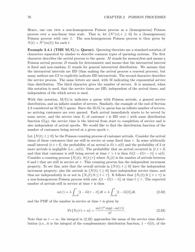
With this notation, M/G/1 indicates a queue with Poisson arrivals, a general servicedistribution, and an infinite number of servers. Similarly, the example at the end of Section2.3 considered an M/M/1 queue. Since the M/G/1 queue has an infinite number of servers,no arriving customers are ever queued. Each arrival immediately starts to be served bysome server, and the service time Yi of customer i is IID over i with some distributionfunction G(y); the service time is the interval from start to completion of service and isalso independent of arrival epochs. We would like to find the distribution function of thenumber of customers being served at a given epoch τ .

Let {N(t); t ≥ 0} be the Poisson counting process of customer arrivals. Consider the arrivaltimes of those customers that are still in service at some fixed time τ . In some arbitrarilysmall interval (t, t + δ], the probability of an arrival is δ∏ + o(δ) and the probability of 2 ormore arrivals is negligible (i.e., o(δ)). The probability that an arrival occurred in (t, t + δ]and that that customer is still being served at time τ > t is then δ∏[1 − G(τ − t)] + o(δ).Consider a counting process {N1(t); 0≤t≤τ} where N1(t) is the number of arrivals between0 and t that are still in service at τ . This counting process has the independent incrementproperty. To see this, note that the overall arrivals in {N(t); t ≥ 0} have the independentincrement property; also the arrivals in {N(t); t ≥ 0} have independent service times, andthus are independently in or not in {N1(t); 0 ≤ t < τ}. It follows that {N1(t); 0 ≤ t < τ} isa non-homogeneous Poisson process with rate ∏[1−G(τ − t)] at time t ≤ τ . The expectednumber of arrivals still in service at time τ is then

m(τ) = ∏

Z τ

t=0[1−G(τ − t)] dt = ∏

Z τ

t=0[1−G(t)] dt. (2.32)

and the PMF of the number in service at time τ is given by

Pr{N1(τ) = n} =m(τ)n exp(−m(τ))

n!. (2.33)

Note that as τ →1, the integral in (2.32) approaches the mean of the service time distri-bution (i.e., it is the integral of the complementary distribution function, 1 − G(t), of the

2.5. CONDITIONAL ARRIVAL DENSITIES AND ORDER STATISTICS 77

✲✟✟✟✟✟

❍❍❍❍❍

✲

✲

N(t)1−G(τ−t)

G(τ−t)

N1(τ) = Customers in service at τ

N(τ)−N1(τ) = Customers departed by τ

Figure 2.8: Poisson arrivals {N(t); t ≥ 0} can be considered to be split in a non-homogeneous way. An arrival at t is split with probability 1−G(τ − t) into a processof customers still in service at τ .

service time). This means that in steady-state (as τ → 1), the distribution of the num-ber in service at τ depends on the service time distribution only through its mean. Thisexample can be used to model situations such as the number of phone calls taking placeat a given epoch. This requires arrivals of new calls to be modeled as a Poisson processand the holding time of each call to be modeled as a random variable independent of otherholding times and of call arrival times. Finally, as shown in Figure 2.8, we can regard{N1(t); 0≤t ≤ τ} as a splitting of the arrival process {N(t); t≥0}. By the same type ofargument as in Section 2.3, the number of customers who have completed service by timeτ is independent of the number still in service.

2.5 Conditional arrival densities and order statistics

A diverse range of problems involving Poisson processes are best tackled by conditioning ona given number n of arrivals in the interval (0, t], i.e., on the event N(t) = n. Because ofthe incremental view of the Poisson process as independent and stationary arrivals in eachincremental interval of the time axis, we would guess that the arrivals should have somesort of uniform distribution given N(t) = n. More precisely, the following theorem showsthat the joint density of S (n) = (S1, S2, . . . , Sn) given N(t) = n is uniform over the region0 < S1 < S2 < · · · < Sn < t.

Theorem 2.6. Let fS(n)|N(t)(s(n) | n) be the joint density of S(n) conditional on N(t) = n.

This density is constant over the region 0 < s1 < · · · < sn < t and has the value

fS(n)|N(t)(s(n) | n) =

n!tn

. (2.34)

Two proofs are given, each illustrative of useful techniques.

Proof 1: Recall that the joint density of the first n + 1 arrivals Sn+1 = (S1 . . . , Sn, Sn+1

with no conditioning is given in (2.14). We first use Bayes law to calculate the joint densityof Sn+1 conditional on N(t) = n.

fS (n+1)|N(t)(s(n+1) | n) pN(t)(n) = pN(t)|S (n+1)(n|s(n+1))fS (n+1)(s(n+1)).

Note that N(t) = n if and only if Sn ≤ t and Sn+1 > t. Thus pN(t)|S (n+1)(n|s(n+1)) is 1 ifSn ≤ t and Sn+1 > t and is 0 otherwise. Restricting attention to the case N(t) = n, Sn ≤ t


and Sn+1 > t,

fS (n+1)|N(t)(s(n+1) | n) =

fS (n+1)(s(n+1))pN(t)(n)

=∏n+1 exp(−∏sn+1)(∏t)n exp(−∏t) /n!

=n!∏ exp(−∏(sn+1 − t)

tn. (2.35)

This is a useful expression, but we are interested in S (n) rather than S (n+1). Thus we breakup the left side of (2.35) as follows:

fS (n+1)|N(t)(s(n+1) | n) = fS (n)|N(t)(s

(n) | n) fSn+1|S (n)N(t)(sn+1|s(n), n).

Conditional on N(t) = n, Sn+1 is the first arrival epoch after t, which by the memorylessproperty is independent of Sn. Thus that final term is simply ∏ exp(−∏(sn+1 − t)) forsn+1 > t. Substituting this into (2.35), the result is (2.34).

Proof 2: This alternative proof derives (2.34) by looking at arrivals in very small incrementsof size δ (see Figure 2.9). For a given t and a given set of n times, 0 < s1 < · · · , < sn < t, wecalculate the probability that there is a single arrival in each of the intervals (si, si + δ], 1 ≤i ≤ n and no other arrivals in the interval (0, t]. Letting A(δ) be this event,

0 s1 s2 s3 t

δ✲ ✛ δ✲ ✛ δ✲ ✛

Figure 2.9: Intervals for arrival density.

Pr{A(δ)} = pN(s1)(0) p eN(s1,s1+δ)(1) p eN(s1+δ,s2)(0) p eN(s2,s2+δ)(1) · · · p eN(sn+δ,t)(0).

The sum of the lengths of the above intervals is t, so if we represent p eN(si,si+δ)(1) as∏δ exp(−∏δ) + o(δ) for each i, then

Pr{A(δ)} = (∏δ)n exp(−∏t) + δn−1o(δ).

The event A(δ) can be characterized as the event that, first, N(t) = n and, second, thatthe n arrivals occur in (si, si+δ] for 1 ≤ i ≤ n. Thus we conclude that

fS (n)|N(t)(s(n)) = lim

δ→0

Pr{A(δ)}δnpN(t)(n)

,

which simplifies to (2.34).

The joint density of the interarrival intervals, X (n) = X1 . . . ,Xn given N(t) = n can befound directly from Theorem 2.6 simply by making the linear transformation X1 = S1

2.5. CONDITIONAL ARRIVAL DENSITIES AND ORDER STATISTICS 79

°°

°°

°°

°° ❅❅

❅❅

❅❅

❅❅s1

s2

❅❅❘

x1

x2

Figure 2.10: Mapping from arrival epochs to interarrival times. Note that incrementalcubes in the arrival space map into parallelepipeds of the same volume in the interarrivalspace.

and Xi = Si − Si−1 for 2 ≤ i ≤ n. The density is unchanged, but the constraint regiontransforms into

Pni=1 Xi < t with Xi > 0 for 1 ≤ i ≤ n (see Figure 2.10).

fX (n)|N(t)(x(n) | n) =

n!tn

for X (n) > 0,Xn

i=1Xi < t. (2.36)

It is also instructive to compare the joint distribution of S (n) conditional on N(t) = n withthe joint distribution of n IID uniformly distributed random variables, U (n) = U1, . . . , Un

on (0, t]. For any point U (n) = u (n), this joint density is

fU (n)(u (n)) = 1/tn for 0 < ui ≤ t, 1 ≤ i ≤ n.

Both fS (n) and fU (n) are uniform over the volume of n-space where they are non-zero, butas illustrated in Figure 2.11 for n = 2, the volume for the latter is n! times larger than thevolume for the former. To explain this more fully, we can define a set of random variablesS1, . . . , Sn, not as arrival epochs in a Poisson process, but rather as the order statisticsfunction of the IID uniform variables U1, . . . , Un; that is

S1 = min(U1, . . . , Un); S2 = 2nd smallest (U1, . . . , Un); etc.

The n-cube is partitioned into n! regions, one where u1 < u2 < · · · < un. For eachpermutation π(i) of the integers 1 to n, there is another region9 where uπ(1) < uπ(2) < · · · <uπ(n). By symmetry, each of these regions has the same volume, which then must be 1/n!of the volume tn of the n-cube.

Each of these n! regions map into the same region of ordered values. Thus these orderstatistics have the same joint probability density function as the arrival epochs S1, . . . , Sn

conditional on N(t) = n. Thus anything we know (or can discover) about order statisticsis valid for arrival epochs given N(t) = n and vice versa.10

9As usual, we are ignoring those points where ui = uj for some i, j, since the set of such points has 0probability.

10There is certainly also the intuitive notion, given n arrivals in (0, t], and given the stationary andindependent increment properties of the Poisson process, that those n arrivals can be viewed as uniformlydistributed. It does not seem worth the trouble, however, to make this precise, since there is no natural wayto associate each arrival with one of the uniform rv’s.


°°

°°

°°

°°♣♣♣♣ ♣♣♣♣ ♣♣♣♣ ♣♣♣♣ ♣♣♣♣♣♣♣♣♣♣♣♣♣ ♣♣♣♣♣♣♣♣♣♣♣♣♣ ♣♣♣♣♣♣♣♣♣♣♣♣♣ ♣♣♣♣♣♣♣♣♣♣♣♣♣f=2/t2

♣♣♣♣ ♣♣♣♣ ♣♣♣♣ ♣♣♣

♣ ♣♣♣♣ ♣♣♣♣ ♣♣♣♣ ♣♣♣♣ ♣♣♣♣♣♣♣♣ ♣♣♣♣ ♣♣♣♣ ♣♣♣♣ ♣♣♣♣ ♣♣♣♣ ♣♣♣♣ ♣♣♣

♣

s1

s2

♣♣♣♣♣♣♣♣♣♣♣♣♣♣♣♣♣♣♣♣♣♣♣♣♣♣♣♣♣♣♣♣♣♣♣♣♣♣♣♣♣♣♣♣♣♣♣♣♣♣♣♣♣♣♣♣♣♣♣♣♣♣♣♣♣♣♣♣♣♣♣♣♣♣♣♣♣♣♣♣♣♣♣♣♣♣♣♣♣♣♣♣♣♣♣♣

♣♣♣♣♣♣♣♣♣♣♣♣♣♣♣♣♣♣♣♣♣♣♣♣♣♣♣♣♣♣♣♣♣♣♣♣♣♣♣♣♣♣♣♣♣♣♣♣♣♣♣♣♣♣♣♣♣♣♣♣♣♣♣♣♣♣♣♣♣♣♣♣♣♣♣♣♣♣♣♣♣♣♣♣♣♣♣♣♣♣♣♣♣♣♣♣

f=1/t2♣♣♣♣♣♣♣♣♣♣♣♣♣♣♣♣♣♣♣♣♣♣♣♣

♣♣♣♣♣♣♣♣♣♣♣♣♣♣♣♣♣♣♣♣♣♣♣♣

u1

u2

0 t0 t0

t

0

t

Figure 2.11: Density for the order statistics of an IID 2 dimensional uniform distri-bution. Note that the square over which fU (2) is non-zero contains one triangle whereu2 > u1 and another of equal size where u1 > u2. Each of these maps, by a permutationmapping, into the single triangle where s2 > s1.

Next we want to find the marginal distribution functions of the individual Si conditional onN(t) = n. Starting with S1, and viewing it as the minimum of the IID uniformly distributedvariables U1, . . . , Un, we recognize that S1 > τ if and only if Ui > τ for all i, 1 ≤ i ≤ n.Thus,

Pr{S1 > τ | N(t)=n} =∑t− τ

t

∏n

for 0 < τ ≤ t. (2.37)

Since this is the complement of the distribution function of S1, conditional on N(t) = n,we can integrate it to get the conditional mean of S1,

E [S1 | N(t)=n] =t

n + 1. (2.38)

We come back later to the distribution functions of S2, . . . , Sn, and first look at the marginaldistributions of the interarrival intervals. Recall from (2.36) that

fX (n)|N(t)(x(n) | n) =

n!tn

for X (n) > 0,Xn

i=1Xi < t. (2.39)

The joint density is the same for all points in the constraint region, and the constraint doesnot distinguish between X1 to Xn. Thus they must all have the same marginal distribution,and more generally the marginal distribution of any subset of the Xi can depend only onthe size of the subset. We have found the distribution of S1, which is the same as X1, andthus

Pr{Xi > τ | N(t)=n} =∑t− τ

t

∏n

for 1 ≤ i ≤ n and 0 < τ ≤ t. (2.40)

E [Xi | N(t)=n] =t

n + 1for 1 ≤ i ≤ n. (2.41)

Next define X∗n+1 = t− Sn to be the interval from the largest of the IID variables to t, the

right end of the interval. Using (2.39)

fX (n)|N(t)(x(n) | n) =

n!tn

for X (n) > 0, X∗n+1 > 0,

Xn

i=1Xi + X∗

n+1 = t.

2.6. SUMMARY 81

The constraints above are symmetric in X1, . . . ,Xn,X∗n+1, and the density of X1, . . . ,Xn

within the constrainty region is uniform. This density can be replaced by a density over anyother n rv’s out of X1, . . . ,Xn,X∗

n+1 by a linear transformation with unit determinant. ThusX∗

n+1 has the same marginal distribution as each of the Xi. This gives us a partial check onour work, since the interval (0, t] is divided into n+1 intervals of sizes X1,X2, . . . ,Xn,X∗

n+1,and each of these has a mean size t/(n+1). We also see that the joint distribution functionof any proper subset of X1,X2, . . .Xn, X∗

n+1 is independent of the order of the variables.

Next consider the distribution function of Xi+1 for (i < n), conditional both on N(t) = nand Si = si (or conditional on any given values for X1, . . . ,Xi summing to si). We seethat Xi+1 is just the wait until the first arrival in the interval (si, t], given that this intervalcontains n− i arrivals. From the same argument as used in (2.37), we have

Pr{Xi+1 > τ | N(t)=n, Si=si} =∑t− si − τ

t− si

∏n−i

. (2.42)

Since Si+1 is Xi+1 + Si, this immediately gives us the conditional distribution of Si+1

Pr{Si+1 > si+1 | N(t) = n, Si = si} =∑t− si+1

t− si

∏n−i

. (2.43)

We note that this is independent of S1, . . . , Si−1. As a check, one can find the conditionaldensities from (2.43) and multiply them all together to get back to (2.34) (see Exercise2.25).

W can also find the distribution of each Si conditioned on N(t) = n but unconditioned onS1, S2, . . . , Si−1. The density for this is calculated by looking at n uniformly distributedrv’s in (0, t]. The probability that one of these lies in the interval (x, x+dt] is (ndt)/t. Outof the remaining n − 1, the probability that i − 1 lie in the interval (0, x] is given by thebinomial distribution with probability of success x/t. Thus the desired density is

fSi (x | N(t)=n) dt =xi−1(t− x)n−i(n− 1)!

tn−1(n− i)!(i− 1)!ndt

t

fSi(x | N(t)=n) =xi−1(t− x)n−in!tn(n− i)!(i− 1)!

. (2.44)

2.6 Summary

We started the chapter with three equivalent definitions of a Poisson process—first as arenewal process with exponentially distributed inter-renewal intervals, second as a station-ary and independent increment counting process with Poisson distributed arrivals in eachinterval, and third essentially as a limit of shrinking Bernoulli processes. We saw that eachdefinition provided its own insights into the properties of the process. We emphasized theimportance of the memoryless property of the exponential distribution, both as a usefultool in problem solving and as an underlying reason why the Poisson process is so simple.

We next showed that the sum of independent Poisson processes is again a Poisson process.We also showed that if the arrivals in a Poisson process are independently routed to different


locations with some fixed probability assignment, then the arrivals at each of these locationsform independent Poisson processes. This ability to view independent Poisson processeseither independently or as a splitting of a combined process is a powerful technique forfinding almost trivial solutions to many problems.

It was next shown that a non-homogeneous Poisson process could be viewed as a (ho-mogeneous) Poisson process on a non-linear time scale. This allows all the properties of(homogeneous) Poisson properties to be applied directly to the non-homogeneous case. Thesimplest and most useful result from this is (2.31), showing that the number of arrivals inany interval has a Poisson PMF. This result was used to show that the number of cus-tomers in service at any given time τ in an M/G/1 queue has a Poisson PMF with a meanapproaching ∏ times the expected service time in the limit as τ →1.

Finally we looked at the distribution of arrivals conditional on n arrivals in the interval(0, t]. It was found that these arrivals had the same joint distribution as the order statisticsof n uniform IID rv’s in (0, t]. By using symmetry and going back and forth betweenthe uniform variables and the Poisson process arrivals, we found the distribution of theinterarrival times, the arrival epochs, and various conditional distributions.

2.7 Exercises

Exercise 2.1. a) Find the Erlang density fSn(t) by convolving fX(x) = ∏ exp(−∏x) withitself n times.

b) Find the moment generating function of X (or find the Laplace transform of fX(x)),and use this to find the moment generating function (or Laplace transform) of Sn = X1 +X2 + · · · + Xn. Invert your result to find fSn(t).

c) Find the Erlang density by starting with (2.14) and then calculating the marginal densityfor Sn.

Exercise 2.2. a) Find the mean, variance, and moment generating function of N(t), asgiven by (2.15).

b) Show by discrete convolution that the sum of two independent Poisson rv’s is againPoisson.

c) Show by using the properties of the Poisson process that the sum of two independentPoisson rv’s must be Poisson.

Exercise 2.3. The purpose of this exercise is to give an alternate derivation of the Poissondistribution for N(t), the number of arrivals in a Poisson process up to time t; let ∏ be therate of the process.

a) Find the conditional probability Pr{N(t) = n | Sn = τ} for all τ ≤ t.

b) Using the Erlang density for Sn, use (a) to find Pr{N(t) = n}.

2.7. EXERCISES 83

Exercise 2.4. Assume that a counting process {N(t); t≥0} has the independent and sta-tionary increment properties and satisfies (2.15) (for all t > 0). Let X1 be the epoch of thefirst arrival and Xn be the interarrival time between the n− 1st and the nth arrival.

a) Show that Pr{X1 > x} = e−∏x.

b) Let Sn−1 be the epoch of the n− 1st arrival. Show that Pr{Xn > x | Sn−1 = τ} = e−∏x.

c) For each n > 1, show that Pr{Xn > x} = e−∏x and that Xn is independent of Sn−1.

d) Argue that Xn is independent of X1,X2, . . .Xn−1.

Exercise 2.5. The point of this exercise is to show that the sequence of PMF’s for thecounting process of a Bernoulli process does not specify the process. In other words, knowingthat N(t) satisfies the binomial distribution for all t does not mean that the process isBernoulli. This helps us understand why the second definition of a Poisson process requiresstationary and independent increments as well as the Poisson distribution for N(t).

a) For a sequence of binary rv’s Y1, Y2, Y3, . . . , in which each rv is 0 or 1 with equalprobability, find a joint distribution for Y1, Y2, Y3 that satisfies the binomial distribution,pN(t)(k) =

°tk

¢2−k for t = 1, 2, 3 and 0 ≤ k ≤, but for which Y1, Y2, Y3 are not independent.

Your solution should contain four 3-tuples with probability 1/8 each, two 3-tuples withprobability 1/4 each, and two 3-tuples with probability 0. Note that by making the sub-sequent arrivals IID and equiprobable, you have an example where N(t) is binomial for allt but the process is not Bernoulli. Hint: Use the binomial for t = 3 to find two 3-tuplesthat must have probability 1/8. Combine this with the binomial for t = 2 to find two other3-tuples with probability 1/8. Finally look at the constraints imposed by the binomialdistribution on the remaining four 3-tuples.

b) Generalize part a) to the case where Y1, Y2, Y3 satisfy Pr{Yi = 1} = q and Pr{Yi = 0} =1− q. Assume q < 1/2 and find a joint distribution on Y1, Y2, Y3 that satisfies the binomialdistribution, but for which the 3-tuple (0, 1, 1) has zero probability.

c) More generally yet, view a joint PMF on binary t-tuples as a non-negative vector in a 2t

dimensional vector space. Each binomial probability pN(τ)(k) =°τk

¢qk(1−q)τ−k constitutes

a linear constraint on this vector. For each τ , show that one of these constraints may bereplaced by the constraint that the components of the vector sum to 1.

d) Using part c), show that at most (t + 1)t/2 + 1 of the binomial constraints are linearlyindependent. Note that this means that the linear space of vectors satisfying these binomialconstraints has dimension at least 2t − (t + 1)t/2 − 1. This linear space has dimension 1for t = 3 explaining the results in parts a) and b). It has a rapidly increasing dimensionalfor t > 3, suggesting that the binomial constraints are relatively ineffectual for constrainingthe joint PMF of a joint distribution. More work is required for the case of t > 3 becauseof all the inequality constraints, but it turns out that this large dimensionality remains.

Exercise 2.6. Let h(x) be a positive function of a real variable that satisfies h(x + t) =h(x) + h(t) and let h(1) = c.


a) Show that for integer k > 0, h(k) = kc.

b) Show that for integer j > 0, h(1/j) = c/j.

c) Show that for all integer k, j, h(k/j) = ck/j.

d) The above parts show that h(x) is linear in positive rational numbers. For very pickymathematicians, this does not guarantee that h(x) is linear in positive real numbers. Showthat if h(x) is also monotonic in x, then h(x) is linear in x > 0.

Exercise 2.7. Assume that a counting process {N(t); t≥0} has the independent and sta-tionary increment properties and, for all t > 0, satisfies

Prn

eN(t, t + δ) = 0o

= 1− ∏δ + o(δ)

Prn

eN(t, t + δ) = 1o

= ∏δ + o(δ)

Prn

eN(t, t + δ) > 1o

= o(δ).

a) Let F0(τ) = Pr{N(τ) = 0} and show that dF0(τ)/dτ = −∏F0(τ).

b) Show that X1, the time of the first arrival, is exponential with parameter ∏.

c) Let Fn(τ) = Prn

eN(t, t + τ) = 0 | Sn−1 = to

and show that dFn(τ)/dτ = −∏Fn(τ).

d) Argue that Xn is exponential with parameter ∏ and independent of earlier arrival times.

Exercise 2.8. Let t > 0 be an arbitrary time, let Z1 be the duration of the interval fromt until the next arrival after t. Let Zm, for each m > 1, be the interarrival time from theepoch of the m− 1st arrival after t until the mth arrival.

a) Given that N(t) = n, explain why Zm = Xm+n for m > 1 and Z1 = Xn+1 − t + Sn.

b) Conditional on N(t) = n and Sn = τ , show that Z1, Z2, . . . are IID.

c) Show that Z1, Z2, . . . are IID.

Exercise 2.9. Consider a “shrinking Bernoulli” approximation Nδ(mδ) = Y1 + · · ·+Ym toa Poisson process as described in Subsection 2.2.5.

a) Show that

Pr{Nδ(mδ) = n} =µ

m

n

∂(∏δ)n(1− ∏δ)m−n.

b) Let t = mδ, and let t be fixed for the remainder of the exercise. Explain why

limδ→0

Pr{Nδ(t) = n} = limm→1

µm

n

∂µ∏t

m

∂n µ1− ∏t

m

∂m−n

.

2.7. EXERCISES 85

where the limit on the left is taken over values of δ that divide t.

c) Derive the following two equalities:

limm→1

µm

n

∂1

mn=

1n!

; and limm→1

µ1− ∏t

m

∂m−n

= e−∏t.

d) Conclude from this that for every t and every n, limδ→0 Pr{Nδ(t)=n} = Pr{N(t)=n}where {N(t); t ≥ 0} is a Poisson process of rate ∏.

Exercise 2.10. Let {N(t); t ≥ 0} be a Poisson process of rate ∏.

a) Find the joint probability mass function (PMF) of N(t), N(t + s) for s > 0.

b) Find E [N(t) · N(t + s)] for s > 0.

c) Find Eh

eN(t1, t3) · eN(t2, t4)i

where eN(t, τ) is the number of arrivals in (t, τ ] and t1 <

t2 < t3 < t4.

Exercise 2.11. An experiment is independently performed N times where N is a Poissonrv of mean ∏. Let {a1, a2, . . . , aK} be the set of sample points of the experiment and letpk, 1 ≤ k ≤ K, denote the probability of ak.

a) Let Ni denote the number of experiments performed for which the output is ai. Findthe PMF for Ni (1 ≤ i ≤ K). (Hint: no calculation is necessary.)

b) Find the PMF for N1 + N2.

c) Find the conditional PMF for N1 given that N = n.

d) Find the conditional PMF for N1 + N2 given that N = n.

e) Find the conditional PMF for N given that N1 = n1.

Exercise 2.12. Starting from time 0, northbound buses arrive at 77 Mass. Avenue accord-ing to a Poisson process of rate ∏. Passengers arrive according to an independent Poissonprocess of rate µ. When a bus arrives, all waiting customers instantly enter the bus andsubsequent customers wait for the next bus.

a) Find the PMF for the number of customers entering a bus (more specifically, for anygiven m, find the PMF for the number of customers entering the mth bus).

b) Find the PMF for the number of customers entering the mth bus given that the inter-arrival interval between bus m− 1 and bus m is x.

c) Given that a bus arrives at time 10:30 PM, find the PMF for the number of customersentering the next bus.

d) Given that a bus arrives at 10:30 PM and no bus arrives between 10:30 and 11, find thePMF for the number of customers on the next bus.


e) Find the PMF for the number of customers waiting at some given time, say 2:30 PM(assume that the processes started infinitely far in the past). Hint: think of what happensmoving backward in time from 2:30 PM.

f) Find the PMF for the number of customers getting on the next bus to arrive after 2:30.(Hint: this is different from part (a); look carefully at part e).

g) Given that I arrive to wait for a bus at 2:30 PM, find the PMF for the number ofcustomers getting on the next bus.

Exercise 2.13. a) Show that the arrival epochs of a Poisson process satisfy

fS (n)|Sn+1(s(n)|sn+1) = n!/sn

n+1.

Hint: This is easy if you use only the results of Section 2.2.2.

b) Contrast this with the result of Theorem 2.6

Exercise 2.14. Equation (2.44) gives fSi(x | N(t)=n), which is the density of randomvariable Si conditional on N(t) = n for n ≥ i. Multiply this expression by Pr{N(t) = n}and sum over n to find fSi(x); verify that your answer is indeed the Erlang density.

Exercise 2.15. Consider generalizing the bulk arrival process in Figure 2.5. Assume thatthe epochs at which arrivals occur form a Poisson process {N(t); t ≥ 0} of rate ∏. At eacharrival epoch, Sn, the number of arrivals, Zn, satisfies Pr{Zn=1} = p, Pr{Zn=2)} = 1− p.The variables Zn are IID.

a) Let {N1(t); t ≥ 0} be the counting process of the epochs at which single arrivals occur.Find the PMF of N1(t) as a function of t. Similarly, let {N2(t); t ≥ 0} be the countingprocess of the epochs at which double arrivals occur. Find the PMF of N2(t) as a functionof t.

b) Let {NB(t); t ≥ 0} be the counting process of the total number of arrivals. Give anexpression for the PMF of NB(t) as a function of t.

Exercise 2.16. a) For a Poisson counting process of rate ∏, find the joint probabilitydensity of S1, S2, . . . , Sn−1 conditional on Sn = t.

b) Find Pr{X1 > τ | Sn=t}.

c) Find Pr{Xi > τ | Sn=t} for 1 ≤ i ≤ n.

d) Find the density fSi(x|Sn=t) for 1 ≤ i ≤ n− 1.

e) Give an explanation for the striking similarity between the condition N(t) = n− 1 andthe condition Sn = t.

2.7. EXERCISES 87

Exercise 2.17. a) For a Poisson process of rate ∏, find Pr{N(t)=n | S1=τ} for t > τ andn ≥ 1.

b) Using this, find fS1(τ | N(t)=n)

c) Check your answer against (2.37).

Exercise 2.18. Consider a counting process in which the rate is a rv Λ with probabilitydensity fΛ(∏) = αe−α∏ for ∏ > 0. Conditional on a given sample value ∏ for the rate, thecounting process is a Poisson process of rate ∏ (i.e., nature first chooses a sample value ∏and then generates a sample function of a Poisson process of that rate ∏).

a) What is Pr{N(t)=n | Λ=∏}, where N(t) is the number of arrivals in the interval (0, t]for some given t > 0?

b) Show that Pr{N(t)=n}, the unconditional PMF for N(t), is given by

Pr{N(t)=n} =αtn

(t + α)n+1.

c) Find fΛ(∏ | N(t)=n), the density of ∏ conditional on N(t)=n.

d) Find E [Λ | N(t)=n] and interpret your result for very small t with n = 0 and for verylarge t with n large.

e) Find E [Λ | N(t)=n, S1, S2, . . . , Sn]. (Hint: consider the distribution of S1, . . . , Sn con-ditional on N(t) and Λ). Find E [Λ | N(t)=n,N(τ)=m] for some τ < t.

Exercise 2.19. a) Use Equation (2.44) to find E [Si | N(t)=n]. Hint: When you integratexfSi(x | N(t)=n), compare this integral with fSi+1(x | N(t)=n + 1) and use the fact thatthe latter expression is a probability density.

b) Find the second moment and the variance of Si conditional on N(t)=n. Hint: Extendthe previous hint.

c) Assume that n is odd, and consider i = (n + 1)/2. What is the relationship between Si,conditional on N(t)=n, and the sample median of n IID uniform random variables.

d) Give a weak law of large numbers for the above median.

Exercise 2.20. Suppose cars enter a one-way infinite length, infinite lane highway at aPoisson rate ∏. The ith car to enter chooses a velocity Vi and travels at this velocity.Assume that the Vi’s are independent positive rv’s having a common distribution F . Derivethe distribution of the number of cars that are located in an interval (0, a) at time t.

Exercise 2.21. Consider an M/G/1 queue, i.e., a queue with Poisson arrivals of rate ∏in which each arrival i, independent of other arrivals, remains in the system for a time Xi,where {Xi; i ≥ 1} is a set of IID rv’s with some given distribution function F (x).


You may assume that the number of arrivals in any interval (t, t + ε) that are still in thesystem at some later time τ ≥ t + ε is statistically independent of the number of arrivals inthat same interval (t, t + ε) that have departed from the system by time τ .

a) Let N(τ) be the number of customers in the system at time τ . Find the mean, m(τ), ofN(τ) and find Pr{N(τ) = n}.

b) Let D(τ) be the number of customers that have departed from the system by time τ .Find the mean, E [D(τ)], and find Pr{D(τ) = d}.

c) Find Pr{N(τ) = n,D(τ) = d}.

d) Let A(τ) be the total number of arrivals up to time τ . Find Pr{N(τ) = n | A(τ) = a}.

e) Find Pr{D(τ + ε)−D(τ) = d}.

Exercise 2.22. The voters in a given town arrive at the place of voting according toa Poisson process of rate ∏ = 100 voters per hour. The voters independently vote forcandidate A and candidate B each with probability 1/2. Assume that the voting starts attime 0 and continues indefinitely.

a) Conditional on 1000 voters arriving during the first 10 hours of voting, find the probabilitythat candidate A receives n of those votes.

b) Again conditional on 1000 voters during the first 10 hours, find the probability thatcandidate A receives n votes in the first 4 hours of voting.

c) Let T be the epoch of the arrival of the first voter voting for candidate A. Find thedensity of T .

d) Find the PMF of the number of voters for candidate B who arrive before the first voterfor A.

e) Define the nth voter as a reversal if the nth voter votes for a different candidate thanthe n− 1st. For example, in the sequence of votes AABAABB, the third, fourth, and sixthvoters are reversals; the third and sixth are A to B reversals and the fourth is a B to Areversal. Let N(t) be the number of reversals up to time t (t in hours). Is {N(t); t ≥ 0} aPoisson process? Explain.

f) Find the expected time (in hours) between reversals.

g) Find the probability density of the time between reversals.

h) Find the density of the time from one A to B reversal to the next A to B reversal.

Exercise 2.23. Let {N1(t); t ≥ 0} be a Poisson counting process of rate ∏. Assume thatthe arrivals from this process are switched on and off by arrivals from a second independentPoisson process {N2(t); t ≥ 0} of rate ∞.

Let {NA(t); t≥0} be the switched process; that is NA(t) includes the arrivals from {N1(t); t ≥0} during periods when N2(t) is even and excludes the arrivals from {N1(t); t ≥ 0} whileN2(t) is odd.

2.7. EXERCISES 89

✁❆ ✁❆ ✁❆ ✁❆ ✁❆ ✁❆ ✁❆ ✁❆

✁❆✛ ✲On✁❆✛ ✲On

✁❆ ✁❆✛ ✲On✁❆

✁❆ ✁❆ ✁❆ ✁❆ NA(t)

N2(t)

N1(t)

rate ∞

rate ∏

a) Find the PMF for the number of arrivals of the first process, {N1(t); t ≥ 0}, during thenth period when the switch is on.

b) Given that the first arrival for the second process occurs at epoch τ , find the conditionalPMF for the number of arrivals of the first process up to τ .

c) Given that the number of arrivals of the first process, up to the first arrival for the secondprocess, is n, find the density for the epoch of the first arrival from the second process.

d) Find the density of the interarrival time for {NA(t); t ≥ 0}. Note: This part is quitemessy and is done most easily via Laplace transforms.

Exercise 2.24. Let us model the chess tournament between Fisher and Spassky as astochastic process. Let Xi, for i ≥ 1, be the duration of the ith game and assume that{Xi; i≥1} is a set of IID exponentially distributed rv’s each with density f(x) = ∏e−∏x.Suppose that each game (independently of all other games, and independently of the lengthof the games) is won by Fisher with probability p, by Spassky with probability q, and is adraw with probability 1−p−q. The first player to win n games is defined to be the winner,but we consider the match up to the point of winning as being embedded in an unendingsequence of games.

a) Find the distribution of time, from the beginning of the match, until the completion ofthe first game that is won (i.e., that is not a draw). Characterize the process of the number{N(t); t ≥ 0} of games won up to and including time t. Characterize the process of thenumber {NF (t); t ≥ 0} of games won by Fisher and the number {NS(t); t ≥ 0} won bySpassky.

b) For the remainder of the problem, assume that the probability of a draw is zero; i.e.,that p + q = 1. How many of the first 2n− 1 games must be won by Fisher in order to winthe match?

c) What is the probability that Fisher wins the match? Your answer should not involveany integrals. Hint: consider the unending sequence of games and use part b.

d) Let T be the epoch at which the match is completed (i.e., either Fisher or Spassky wins).Find the distribution function of T .

e) Find the probability that Fisher wins and that T lies in the interval (t, t+δ) for arbitrarilysmall δ.

Exercise 2.25. Using (2.43), find the conditional density of Si+1, conditional on N(t) = nand Si = si, and use this to find the joint density of S1, . . . , Sn conditional on N(t) = n.Verify that your answer agrees with (2.34).


Exercise 2.26. A two-dimensional Poisson process is a process of randomly occurring spe-cial points in the plane such that (i) for any region of area A the number of special points inthat region has a Poisson distribution with mean ∏A, and (ii) the number of special pointsin nonoverlapping regions is independent. For such a process consider an arbitrary locationin the plane and let X denote its distance from its nearest special point (where distance ismeasured in the usual Euclidean manner). Show that

a) Pr{X > t} = exp(−∏πt2)

b) E [X] = 1/(2√

∏).

Exercise 2.27. This problem is intended to show that one can analyze the long termbehavior of queueing problems by using just notions of means and variances, but that suchanalysis is awkward, justifying understanding the strong law of large numbers. Consider anM/G/1 queue. The arrival process is Poisson with ∏ = 1. The expected service time, E [Y ],is 1/2 and the variance of the service time is given to be 1.

a) Consider Sn, the time of the nth arrival, for n = 1012. With high probability, Sn will liewithin 3 standard derivations of its mean. Find and compare this mean and the 3σ range.

b) Let Vn be the total amount of time during which the server is busy with these n arrivals(i.e., the sum of 1012 service times). Find the mean and 3σ range of Vn.

c) Find the mean and 3σ range of In, the total amount of time the server is idle up untilSn (take In as Sn − Vn, thus ignoring any service time after Sn).

d) An idle period starts when the server completes a service and there are no waitingarrivals; it ends on the next arrival. Find the mean and variance of an idle period. Aresuccessive idle periods IID?

e) Combine (c) and (d) to estimate the total number of idle periods up to time Sn. Usethis to estimate the total number of busy periods.

f) Combine (e) and (b) to estimate the expected length of a busy period.

Exercise 2.28. The purpose of this problem is to illustrate that for an arrival process withindependent but not identically distributed interarrival intervals, X1,X2, . . . ,, the numberof arrivals N(t) in the interval (0, t] can be a defective rv. In other words, the ‘countingprocess’ is not a stochastic process according to our definitions. This illustrates that it isnecessary to prove that the counting rv’s for a renewal process are actually rv’s .

a) Let the distribution function of the ith interarrival interval for an arrival process beFXi(xi) = 1− exp(−αixi) for some fixed α ∈ (0, 1). Let Sn = X1 + · · ·Xn and show that

E [Sn] =1− αn−1

1− α.

b) Sketch a ‘reasonable’ sample function for N(t).

c) Find σ2Sn

.

2.7. EXERCISES 91

d) Use the Chebyshev inequality on Pr{Sn ≥ t} to find an upper bound on Pr{N(t) ≤ n}that is smaller than 1 for all n and for large enough t. Use this to show that N(t) is defectivefor large enough t.

Documents

POISSON PROCESSES - RLE at · PDF fileChapter 2 POISSON PROCESSES 2.1 Introduction A Poisson process is a simple and widely used stochastic process for modeling the times at which