Embed Size (px)
Citation preview

Polar CodingPart 1 - Background
Erdal Arıkan
Electrical-Electronics Engineering Department,Bilkent University, Ankara, Turkey
Algorithmic Coding Theory WorkshopJune 13 - 17, 2016
ICERM, Providence, RI

Outline
Sequential decoding and the cutoff rate
Guessing and cutoff rate
Boosting the cutoff rate
Pinsker’s scheme
Massey’s scheme
Polar coding

Sequential decoding and the cutoff rate
Guessing and cutoff rate
Boosting the cutoff rate
Pinsker’s scheme
Massey’s scheme
Polar coding
Sequential decoding and the cutoff rate 1 / 72

Tree coding and sequential decoding (SD)
I Consider a tree code (ofrate 1/2)
I A path is chosen andtransmitted
I Given the channel output,search the tree for thecorrect (transmitted) path
I The tree structure turnsthe ML decoding probleminto a tree search problem
I A depth-first searchalgorithm exists calledsequential decoding (SD)
0
1
Transmitted path
00
11
00
11
10
01
00
11
10
01
11
00
01
10
00
11
10
01
11
00
01
10
00
11
10
01
11
00
01
10
Sequential decoding and the cutoff rate 2 / 72
Tree coding and sequential decoding (SD)
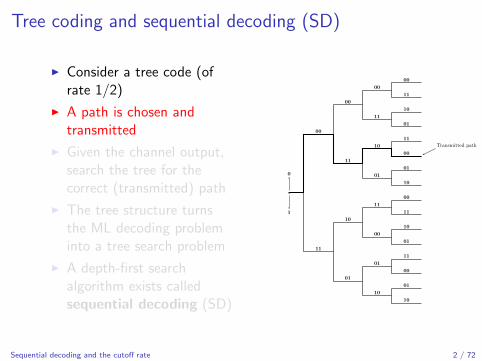
I Consider a tree code (ofrate 1/2)
I A path is chosen andtransmitted
I Given the channel output,search the tree for thecorrect (transmitted) path
I The tree structure turnsthe ML decoding probleminto a tree search problem
I A depth-first searchalgorithm exists calledsequential decoding (SD)
0
1
Transmitted path
00
11
00
11
10
01
00
11
10
01
11
00
01
10
00
11
10
01
11
00
01
10
00
11
10
01
11
00
01
10
Sequential decoding and the cutoff rate 2 / 72

Tree coding and sequential decoding (SD)
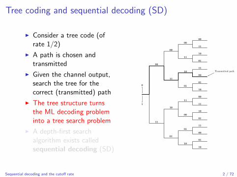
I Consider a tree code (ofrate 1/2)
I A path is chosen andtransmitted
I Given the channel output,search the tree for thecorrect (transmitted) path
I The tree structure turnsthe ML decoding probleminto a tree search problem
I A depth-first searchalgorithm exists calledsequential decoding (SD)
0
1
Transmitted path
00
11
00
11
10
01
00
11
10
01
11
00
01
10
00
11
10
01
11
00
01
10
00
11
10
01
11
00
01
10
Sequential decoding and the cutoff rate 2 / 72
Tree coding and sequential decoding (SD)
I Consider a tree code (ofrate 1/2)
I A path is chosen andtransmitted
I Given the channel output,search the tree for thecorrect (transmitted) path
I The tree structure turnsthe ML decoding probleminto a tree search problem
I A depth-first searchalgorithm exists calledsequential decoding (SD)
0
1
Transmitted path
00
11
00
11
10
01
00
11
10
01
11
00
01
10
00
11
10
01
11
00
01
10
00
11
10
01
11
00
01
10
Sequential decoding and the cutoff rate 2 / 72

Search metric
SD uses a “metric” to distinguishthe correct path from theincorrect ones
Fano’s metric:
Γ(yn, xn) = logP(yn|xn)
P(yn)− nR
path length ncandidate path xn
received sequence yn
code rate R
Sequential decoding and the cutoff rate 3 / 72

HistoryI Tree codes were introduced by Elias (1955) with the aim of
reducing the complexity of ML decoding (the tree structuremakes it possible to use search heuristics for ML decoding)
I Sequential decoding was introduced by Wozencraft (1957) aspart of his doctoral thesis
I Fano (1963) simplified the search algorithm and introducedthe above metric
Sequential decoding and the cutoff rate 4 / 72

Drift properties of the metric
I On the correct path, the expectation of the metric perchannel symbol is∑
y ,x
p(x , y)
[log
p(y |x)
P(y)− R
]= I (X ;Y )− R.
I On any incorrect path, the expectation is∑x ,y
p(x)p(y)
[log
p(y |x)
p(y)− R
]≤ −R
I A properly designed SD scheme – given enough time –identifies the correct path with probability one at any rateR < I (X ;Y ).
Sequential decoding and the cutoff rate 5 / 72
Computation problem in sequential decoding
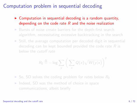
I Computation in sequential decoding is a random quantity,depending on the code rate R and the noise realization
I Bursts of noise create barriers for the depth-first searchalgorithm, necessitating excessive backtracking in the search
I Still, the average computation per decoded digit in sequentialdecoding can be kept bounded provided the code rate R isbelow the cutoff rate
R0∆= − log
∑y
(∑x
Q(x)√W (y |x)
)2
I So, SD solves the coding problem for rates below R0
I Indeed, SD was the method of choice in spacecommunications, albeit briefly
Sequential decoding and the cutoff rate 6 / 72

Computation problem in sequential decoding
I Computation in sequential decoding is a random quantity,depending on the code rate R and the noise realization
I Bursts of noise create barriers for the depth-first searchalgorithm, necessitating excessive backtracking in the search
I Still, the average computation per decoded digit in sequentialdecoding can be kept bounded provided the code rate R isbelow the cutoff rate
R0∆= − log
∑y
(∑x
Q(x)√W (y |x)
)2
I So, SD solves the coding problem for rates below R0
I Indeed, SD was the method of choice in spacecommunications, albeit briefly
Sequential decoding and the cutoff rate 6 / 72
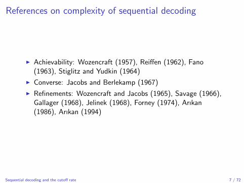
References on complexity of sequential decoding
I Achievability: Wozencraft (1957), Reiffen (1962), Fano(1963), Stiglitz and Yudkin (1964)
I Converse: Jacobs and Berlekamp (1967)
I Refinements: Wozencraft and Jacobs (1965), Savage (1966),Gallager (1968), Jelinek (1968), Forney (1974), Arıkan(1986), Arıkan (1994)
Sequential decoding and the cutoff rate 7 / 72

Sequential decoding and the cutoff rate
Guessing and cutoff rate
Boosting the cutoff rate
Pinsker’s scheme
Massey’s scheme
Polar coding
Guessing and cutoff rate 8 / 72

A computational model for sequential decoding
I SD visits nodes at level N in a certain order
I No “look-ahead” assumption: SD forgets what it saw beyondlevel N upon backtracking
I Complexity measure GN : The number of nodes searched(visited) at level N until the correct node is visited for the firsttime
Guessing and cutoff rate 9 / 72

A bound of computational complexity
I Let R be a fixed code rate.
I There exist tree codes of rate R such that
E [GN ] ≤ 1 + 2−N(R0−R).
I Conversely, for any tree code of rate R,
E [GN ] & 1 + 2−N(R0−R)
Guessing and cutoff rate 10 / 72

A bound of computational complexity
I Let R be a fixed code rate.
I There exist tree codes of rate R such that
E [GN ] ≤ 1 + 2−N(R0−R).
I Conversely, for any tree code of rate R,
E [GN ] & 1 + 2−N(R0−R)
Guessing and cutoff rate 10 / 72

A bound of computational complexity
I Let R be a fixed code rate.
I There exist tree codes of rate R such that
E [GN ] ≤ 1 + 2−N(R0−R).
I Conversely, for any tree code of rate R,
E [GN ] & 1 + 2−N(R0−R)
Guessing and cutoff rate 10 / 72

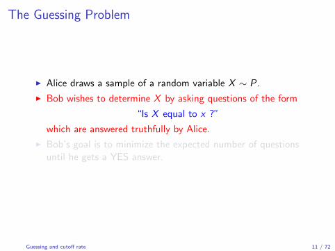
The Guessing Problem
I Alice draws a sample of a random variable X ∼ P.
I Bob wishes to determine X by asking questions of the form
“Is X equal to x ?”
which are answered truthfully by Alice.
I Bob’s goal is to minimize the expected number of questionsuntil he gets a YES answer.
Guessing and cutoff rate 11 / 72

Guessing with Side Information
I Alice samples (X ,Y ) ∼ P(x , y).
I Bob observes Y and is to determine X by asking the sametype of questions
“Is X equal to x ?”
I The goal is to minimize the expected number of quesses.
Guessing and cutoff rate 12 / 72

Guessing with Side Information
I Alice samples (X ,Y ) ∼ P(x , y).
I Bob observes Y and is to determine X by asking the sametype of questions
“Is X equal to x ?”
I The goal is to minimize the expected number of quesses.
Guessing and cutoff rate 12 / 72

Guessing with Side Information
I Alice samples (X ,Y ) ∼ P(x , y).
I Bob observes Y and is to determine X by asking the sametype of questions
“Is X equal to x ?”
I The goal is to minimize the expected number of quesses.
Guessing and cutoff rate 12 / 72

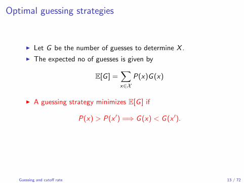
Optimal guessing strategies
I Let G be the number of guesses to determine X .
I The expected no of guesses is given by
E[G ] =∑x∈X
P(x)G (x)
I A guessing strategy minimizes E[G ] if
P(x) > P(x ′) =⇒ G (x) < G (x ′).
Guessing and cutoff rate 13 / 72

Optimal guessing strategies
I Let G be the number of guesses to determine X .
I The expected no of guesses is given by
E[G ] =∑x∈X
P(x)G (x)
I A guessing strategy minimizes E[G ] if
P(x) > P(x ′) =⇒ G (x) < G (x ′).
Guessing and cutoff rate 13 / 72
Optimal guessing strategies
I Let G be the number of guesses to determine X .
I The expected no of guesses is given by
E[G ] =∑x∈X
P(x)G (x)
I A guessing strategy minimizes E[G ] if
P(x) > P(x ′) =⇒ G (x) < G (x ′).
Guessing and cutoff rate 13 / 72

Upper bound on guessing effort
For any optimal guessing function
E[G ∗(X )] ≤[∑
x
√P(x)
]2
Proof.
G ∗(x) ≤∑all x ′
√P(x ′)/P(x) =
M∑i=1
ipG (i)
E[G ∗(X )] ≤∑x
P(x)∑x ′
√P(x ′)/P(x) =
[∑x
√P(x)
]2
.
Guessing and cutoff rate 14 / 72
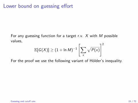
Lower bound on guessing effort
For any guessing function for a target r.v. X with M possiblevalues,
E[G (X )] ≥ (1 + lnM)−1
[∑x
√P(x)
]2
For the proof we use the following variant of Holder’s inequality.
Guessing and cutoff rate 15 / 72

Lemma
Let ai , pi be positive numbers.
∑i
aipi ≥[∑
i
a−1i
]−1 [∑i
√pi
]2
.
Proof. Let λ = 1/2 and put Ai = a−1i , Bi = aλi p
λi , in Holder’s
inequality
∑i
AiBi ≤[∑
i
A1/(1−λ)i
]1−λ [∑i
B1/λi
]λ.
Guessing and cutoff rate 16 / 72

Proof of Lower Bound
E[G (X ) =M∑i=1
ipG (i)
≥(
M∑i=1
1/i
)−1( M∑i=1
√pG (i)
)2
=
(M∑i=1
1/i
)−1(∑x
√P(x)
)2
≥ (1 + lnM)−1
(∑x
√P(x)
)2
Guessing and cutoff rate 17 / 72

Essense of the inequalities
For any set of real numbers p1 ≥ p2 ≥ · · · ≥ pM > 0,
1 ≥∑M
i=1 i pi[∑Mi=1
√pi
]2≥ (1 + lnM)−1
Guessing and cutoff rate 18 / 72

Guessing Random Vectors
I Let X = (X1, . . . ,Xn) ∼ P(x1, . . . , xn).
I Guessing X means asking questions of the form
“Is X = x ?”
for possible values x = (x1, . . . , xn) of X.
I Notice that coordinate-wise probes of the type
“Is Xi = xi ?”
are not allowed.
Guessing and cutoff rate 19 / 72

Complexity of Vector Guessing
Suppose Xi has Mi possible values, i = 1, . . . , n. Then,
1 ≥ E[G ∗(X1, . . . ,Xn)][∑x1,...,xn
√P(x1, . . . , xn)
]2≥ [1 + ln(M1 · · ·Mn)]−1
In particular, if X1, . . . ,Xn are i.i.d. ∼ P with a common alphabetX ,
1 ≥ E[G ∗(X1, . . . ,Xn)][∑x∈X
√P(x)
]2n≥ [1 + n ln |X |]−1
Guessing and cutoff rate 20 / 72

Guessing with Side Information
I (X ,Y ) a pair of random variables with a joint distributionP(x , y).
I Y known. X to be guessed as before.
I G (x |y) the number of guesses when X = x , Y = y .
Guessing and cutoff rate 21 / 72

Lower Bound
For any guessing strategy and any ρ > 0,
E[G (X |Y )] ≥ (1 + lnM)−1∑y
[∑x
√P(x , y)
]2
where M is the number of possible values of X .
Proof. E[G (X |Y )] =∑y
P(y)E[G (X |Y = y)]
≥∑y
P(y)(1 + lnM)−1
[∑x
√P(x |y)
]2
= (1 + lnM)−1∑y
[∑x
√P(x , y)
]2
Guessing and cutoff rate 22 / 72
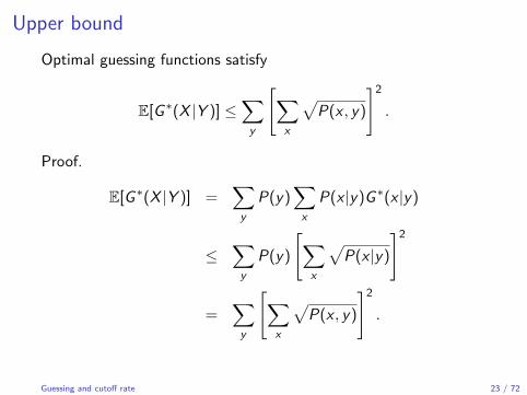
Upper bound
Optimal guessing functions satisfy
E[G ∗(X |Y )] ≤∑y
[∑x
√P(x , y)
]2
.
Proof.
E[G ∗(X |Y )] =∑y
P(y)∑x
P(x |y)G ∗(x |y)
≤∑y
P(y)
[∑x
√P(x |y)
]2
=∑y
[∑x
√P(x , y)
]2
.
Guessing and cutoff rate 23 / 72

Generalization to Random Vectors
For optimal guessing functions, for ρ > 0,
1 ≥ E[G ∗(X1, . . . ,Xk |Y1, . . . ,Yn)]∑y1,...,yn
[∑x1,...,xk
√P(x1, . . . , xk , y1, . . . , yn)
]2
≥ [1 + ln(M1 · · ·Mk)]−1
where Mi denotes the number of possible values of Xi .
Guessing and cutoff rate 24 / 72

A “guessing” decoder
I Consider a block code with M codewords x1, . . . , xM of blocklength N.
I Suppose a codeword is chosen at random and sent over achannel W
I Given the channel output y, a “guessing decoder” decodes byasking questions of the form
“Is the correct codeword the mth one?”
to which it receives a truthful YES or NO answer.
I On a NO answer it repeats the question with a new m.
I The complexity C for this decoder is the number of questionsuntil a YES answer.
Guessing and cutoff rate 25 / 72

Optimal guessing decoder
An optimal guessing decoder is one that minimizes the expectedcomplexity E [C ].Clearly, E [C ] is minimized by generating the guesses in decreasingorder of likelihoods W (y|xm).
xi1 ← 1st guess (the most likely codeword given y)
xi2 ← 2nd guess (2nd most likely codeword given y)
...
xL ← correct codeword obtained; guessing stops
Complexity C equals the number of guesses L
Guessing and cutoff rate 26 / 72
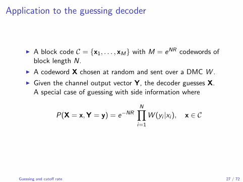
Application to the guessing decoder
I A block code C = {x1, . . . , xM} with M = eNR codewords ofblock length N.
I A codeword X chosen at random and sent over a DMC W .
I Given the channel output vector Y, the decoder guesses X.A special case of guessing with side information where
P(X = x,Y = y) = e−NRN∏i=1
W (yi |xi ), x ∈ C
Guessing and cutoff rate 27 / 72

Cutoff rate bound
E[G ∗(X|Y)] ≥ [1 + NR]−1∑y
[∑x
√P(x, y)
]2
= [1 + NR]−1 eNR∑y
[∑x
QN(x)√WN(x, y)
]2N
≥ [1 + NR]−1 eN(R−R0(W ))
where
R0(W ) = maxQ
− ln∑y
[∑x
Q(x)√W (y |x)
]2
is the channel cutoff rate.
Guessing and cutoff rate 28 / 72

Sequential decoding and the cutoff rate
Guessing and cutoff rate
Boosting the cutoff rate
Pinsker’s scheme
Massey’s scheme
Polar coding
Boosting the cutoff rate 29 / 72

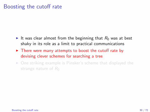
Boosting the cutoff rate
I It was clear almost from the beginning that R0 was at bestshaky in its role as a limit to practical communications
I There were many attempts to boost the cutoff rate bydevising clever schemes for searching a tree
I One striking example is Pinsker’s scheme that displayed thestrange nature of R0
Boosting the cutoff rate 30 / 72

Sequential decoding and the cutoff rate
Guessing and cutoff rate
Boosting the cutoff rate
Pinsker’s scheme
Massey’s scheme
Polar coding
Pinsker’s scheme 31 / 72
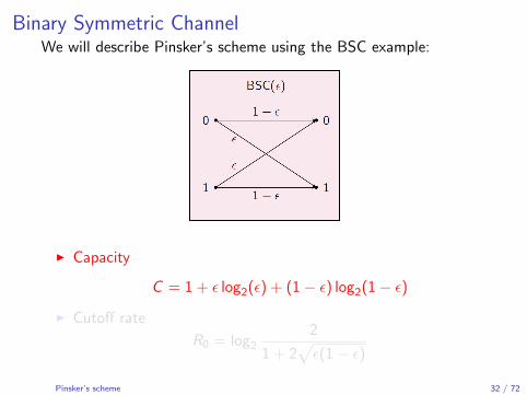
Binary Symmetric ChannelWe will describe Pinsker’s scheme using the BSC example:
I Capacity
C = 1 + ε log2(ε) + (1− ε) log2(1− ε)I Cutoff rate
R0 = log22
1 + 2√ε(1− ε)
Pinsker’s scheme 32 / 72

Binary Symmetric ChannelWe will describe Pinsker’s scheme using the BSC example:
I Capacity
C = 1 + ε log2(ε) + (1− ε) log2(1− ε)I Cutoff rate
R0 = log22
1 + 2√ε(1− ε)
Pinsker’s scheme 32 / 72

Capacity and cutoff rate for the BSC
R0 and C R0/C
Pinsker’s scheme 33 / 72

Pinsker’s scheme
Based on the observations thatas ε→ 0
R0(ε)
C (ε)→ 1 and R0(ε)→ 1,
Pinsker (1965) proposedconcatenation scheme thatachieved capacity withinconstant average cost perdecoded bit irrespective of thelevel of reliability
Pinsker’s scheme 34 / 72

Pinsker’s scheme
d1CE1
u1 u1SD1
d1
x1W
y1
d2CE2
u2 u2SD2
d2
x2W
y2
dK2CEK2
uK2uK2
SDK2
dK2
xN2
WyN2
Blockencoder
Blockdecoder(ML)
K2 identicalconvolutional
encodersN2 independent
copies of W
K2 independentsequential decoders
b
b
b
b
b
b
b
b
b
b
b
The inner block code does the initial clean-up at huge but finitecomplexity; the outer convolutional encoding (CE) and sequential
decoding (SD) boosts the reliability at little extra cost.
Pinsker’s scheme 35 / 72

Discussion
I Although Pinsker’s scheme made a very strong theoreticalpoint, it was not practical.
I There were many more attempts to go around the R0 barrierin 1960s:
I D. Falconer, “A Hybrid Sequential and Algebraic DecodingScheme,” Sc.D. thesis, Dept. of Elec. Eng., M.I.T., 1966.
I I. Stiglitz, Iterative sequential decoding, IEEE Transactions onInformation Theory, vol. 15, no. 6, pp. 715721, Nov. 1969.
I F. Jelinek and J. Cocke, “Bootstrap hybrid decoding forsymmetrical binary input channels,” Inform. Contr., vol. 18,no. 3, pp. 261-298, Apr. 1971.
I It is fair to say that none of these schemes had any practicalimpact
Pinsker’s scheme 36 / 72
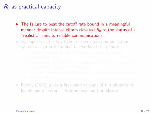
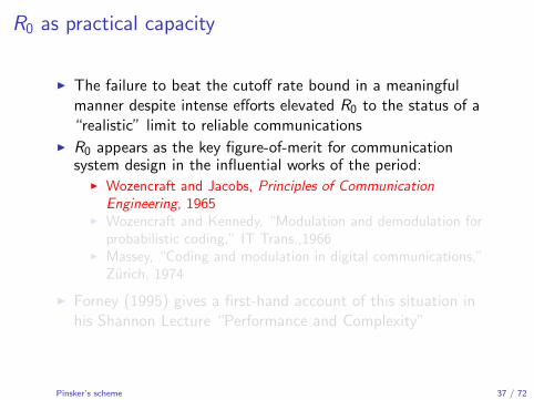
R0 as practical capacity
I The failure to beat the cutoff rate bound in a meaningfulmanner despite intense efforts elevated R0 to the status of a“realistic” limit to reliable communications
I R0 appears as the key figure-of-merit for communicationsystem design in the influential works of the period:
I Wozencraft and Jacobs, Principles of CommunicationEngineering, 1965
I Wozencraft and Kennedy, “Modulation and demodulation forprobabilistic coding,” IT Trans.,1966
I Massey, “Coding and modulation in digital communications,”Zurich, 1974
I Forney (1995) gives a first-hand account of this situation inhis Shannon Lecture “Performance and Complexity”
Pinsker’s scheme 37 / 72

Other attempts to boost the cutoff rate
Efforts to beat the cutoff rate continues to this day
I D. J. Costello and F. Jelinek, 1972.
I P. R. Chevillat and D. J. Costello Jr., 1977.
I F. Hemmati, 1990.
I B. Radosavljevic, E. Arıkan, B. Hajek, 1992.
I J. Belzile and D. Haccoun, 1993.
I S. Kallel and K. Li, 1997.
I E. Arıkan, 2006
I ...
In fact, polar coding originates from such attempts.
Pinsker’s scheme 38 / 72

Sequential decoding and the cutoff rate
Guessing and cutoff rate
Boosting the cutoff rate
Pinsker’s scheme
Massey’s scheme
Polar coding
Massey’s scheme 39 / 72
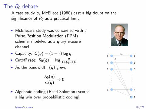
The R0 debateA case study by McEliece (1980) cast a big doubt on thesignificance of R0 as a practical limit
I McEliece’s study was concerned with aPulse Position Modulation (PPM)scheme, modeled as a q-ary erasurechannel
I Capacity: C (q) = (1− ε) log q
I Cutoff rate: R0(q) = log q1+(q−1)ε
I As the bandwidth (q) grew,
R0(q)
C (q)→ 0
I Algebraic coding (Reed-Solomon) scoreda big win over probabilistic coding!
2
3
q
1
2
3
q
1
?
1−ε
ε
Massey’s scheme 40 / 72

The R0 debateA case study by McEliece (1980) cast a big doubt on thesignificance of R0 as a practical limit
I McEliece’s study was concerned with aPulse Position Modulation (PPM)scheme, modeled as a q-ary erasurechannel
I Capacity: C (q) = (1− ε) log q
I Cutoff rate: R0(q) = log q1+(q−1)ε
I As the bandwidth (q) grew,
R0(q)
C (q)→ 0
I Algebraic coding (Reed-Solomon) scoreda big win over probabilistic coding!
2
3
q
1
2
3
q
1
?
1−ε
ε
Massey’s scheme 41 / 72

Massey meets the challenge
I Massey (1981) showed that there was adifferent way of doing coding andmodulation on a q-ary erasure channelthat boosted R0 effortlessly
I Paradoxically, as Massey restored thestatus of R0, he exhibited the “flaky”nature of this parameter
Massey’s scheme 42 / 72

Massey meets the challenge
I Massey (1981) showed that there was adifferent way of doing coding andmodulation on a q-ary erasure channelthat boosted R0 effortlessly
I Paradoxically, as Massey restored thestatus of R0, he exhibited the “flaky”nature of this parameter
Massey’s scheme 42 / 72

Channel splitting to boost cutoff rate (Massey, 1981)
2
3
4
1
2
3
4
1
?
1−ε
ε
1−ε
ε00
01
10
11 11
10
01
00
??
1−εε
0
1 1
0
?
1−εε
0
1 1
0
?
I Begin with a quaternary erasure channel (QEC)
Massey’s scheme 43 / 72

Channel splitting to boost cutoff rate (Massey, 1981)
2
3
4
1
2
3
4
1
?
1−ε
ε
1−ε
ε00
01
10
11 11
10
01
00
??
1−εε
0
1 1
0
?
1−εε
0
1 1
0
?
I Relabel the inputs
Massey’s scheme 44 / 72

Channel splitting to boost cutoff rate (Massey, 1981)
2
3
4
1
2
3
4
1
?
1−ε
ε
1−ε
ε00
01
10
11 11
10
01
00
??
1−εε
0
1 1
0
?
1−εε
0
1 1
0
?
I Split the QEC into two binary erasure channels (BEC)
I BECs fully correlated: erasures occur jointly
Massey’s scheme 45 / 72
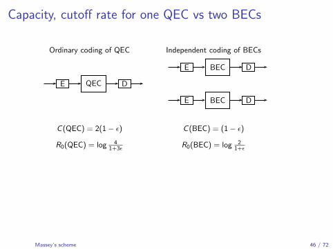
Capacity, cutoff rate for one QEC vs two BECs
Ordinary coding of QEC
C (QEC) = 2(1− ε)
R0(QEC) = log 41+3ε
E QEC D
Independent coding of BECs
C (BEC) = (1− ε)
R0(BEC) = log 21+ε
E BEC D
E BEC D
I C (QEC) = 2× C (BEC)
I R0(QEC) ≤ 2× R0(BEC) with equality iff ε = 0 or 1.
Massey’s scheme 46 / 72

Capacity, cutoff rate for one QEC vs two BECs
Ordinary coding of QEC
C (QEC) = 2(1− ε)
R0(QEC) = log 41+3ε
E QEC D
Independent coding of BECs
C (BEC) = (1− ε)
R0(BEC) = log 21+ε
E BEC D
E BEC D
I C (QEC) = 2× C (BEC)
I R0(QEC) ≤ 2× R0(BEC) with equality iff ε = 0 or 1.
Massey’s scheme 46 / 72

Capacity, cutoff rate for one QEC vs two BECs
Ordinary coding of QEC
C (QEC) = 2(1− ε)
R0(QEC) = log 41+3ε
E QEC D
Independent coding of BECs
C (BEC) = (1− ε)
R0(BEC) = log 21+ε
E BEC D
E BEC D
I C (QEC) = 2× C (BEC)
I R0(QEC) ≤ 2× R0(BEC) with equality iff ε = 0 or 1.
Massey’s scheme 46 / 72

Cutoff rate improvement by splitting
erasure probability (ǫ)0 10
1
2ca
paci
tyan
dcu
toff
rate
(bits
) QEC capacity
QEC cutoff rate
2× BEC cutoff rate
Massey’s scheme 47 / 72

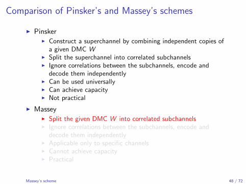
Comparison of Pinsker’s and Massey’s schemes
I PinskerI Construct a superchannel by combining independent copies of
a given DMC WI Split the superchannel into correlated subchannelsI Ignore correlations between the subchannels, encode and
decode them independentlyI Can be used universallyI Can achieve capacityI Not practical
I MasseyI Split the given DMC W into correlated subchannelsI Ignore correlations between the subchannels, encode and
decode them independentlyI Applicable only to specific channelsI Cannot achieve capacityI Practical
Massey’s scheme 48 / 72

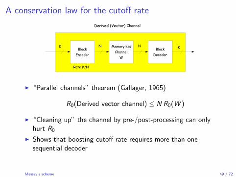
A conservation law for the cutoff rate
MemorylessChannel
W
Derived (Vector) Channel
BlockEncoder
BlockDecoder
N NK K
Rate K/N
I “Parallel channels” theorem (Gallager, 1965)
R0(Derived vector channel) ≤ N R0(W )
I “Cleaning up” the channel by pre-/post-processing can onlyhurt R0
I Shows that boosting cutoff rate requires more than onesequential decoder
Massey’s scheme 49 / 72

Sequential decoding and the cutoff rate
Guessing and cutoff rate
Boosting the cutoff rate
Pinsker’s scheme
Massey’s scheme
Polar coding
Polar coding 50 / 72

Prescription for a new scheme
I Consider small constructions
I Retain independent encoding for the subchannels
I Do not ignore correlations between subchannels at theexpense of capacity
I This points to multi-level coding and successive cancellationdecoding
Polar coding 51 / 72
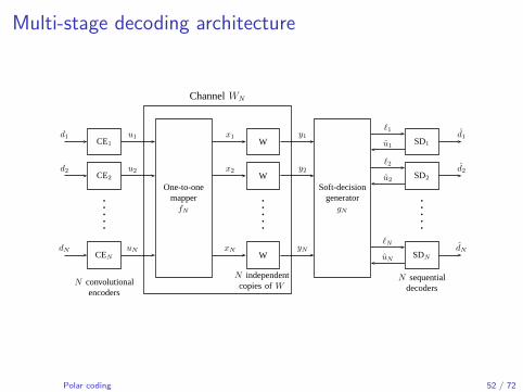
Multi-stage decoding architecture
d1CE1
u1 x1W
y1ℓ1
u1SD1
d1
d2CE2
u2 x2W
y2ℓ2
u2SD2
d2
dNCEN
uN xNW
yNℓN
uNSDN
dN
One-to-onemapperfN
Soft-decisiongenerator
gN
N convolutionalencoders
N independentcopies of W
N sequentialdecoders
b
b
b
b
b
b
b
b
b
b
b
b
b
b
b
Channel WN
Polar coding 52 / 72

Prescription for a new scheme
I Consider small constructions
I Retain independent encoding for the subchannels
I Do not ignore correlations between subchannels at theexpense of capacity
I This points to multi-level coding and successive cancellationdecoding
Polar coding 53 / 72

Notation
I Let V : F2∆= {0, 1} → Y be an arbitrary binary-input
memoryless channel
I Let (X ,Y ) be an input-output ensemble for channel V withX uniform on F2
I The (symmetric) capacity is defined as
I (V )∆= I (X ;Y )
∆=∑y∈Y
∑x∈F2
12V (y |x) log
V (y |x)12V (y |0) + 1
2V (y |1)
I The (symmetric) cutoff rate is defined as
R0(V )∆= R0(X ;Y )
∆= − log
∑y∈Y
∑x∈F2
12
√V (y |x)
2
Polar coding 54 / 72

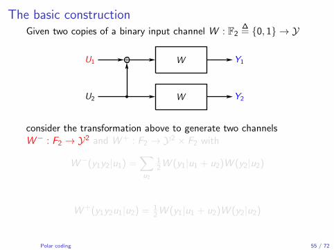
The basic constructionGiven two copies of a binary input channel W : F2
∆= {0, 1} → Y
W
WX1
X2
Y1
Y2
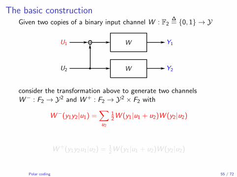
consider the transformation above to generate two channelsW− : F2 → Y2 and W+ : F2 → Y2 × F2 with
W−(y1y2|u1) =∑u2
12W (y1|u1 + u2)W (y2|u2)
W+(y1y2u1|u2) = 12W (y1|u1 + u2)W (y2|u2)
Polar coding 55 / 72

The basic constructionGiven two copies of a binary input channel W : F2
∆= {0, 1} → Y
W
WU1
U2
+ Y1
Y2
consider the transformation above to generate two channelsW− : F2 → Y2 and W+ : F2 → Y2 × F2 with
W−(y1y2|u1) =∑u2
12W (y1|u1 + u2)W (y2|u2)
W+(y1y2u1|u2) = 12W (y1|u1 + u2)W (y2|u2)
Polar coding 55 / 72

The 2x2 transformation is information lossless
I With independent, uniform U1,U2,
I (W−) = I (U1;Y1Y2),
I (W+) = I (U2;Y1Y2U1).
I Thus,
I (W−) + I (W+) = I (U1U2;Y1Y2)
= 2I (W ),
I and I (W−) ≤ I (W ) ≤ I (W+).
Polar coding 56 / 72

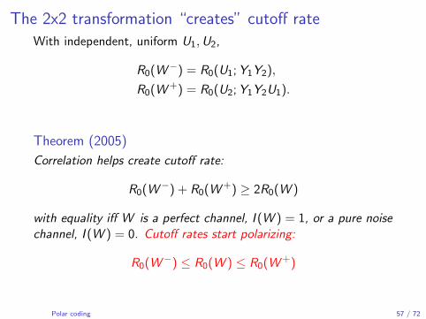
The 2x2 transformation “creates” cutoff rate
With independent, uniform U1,U2,
R0(W−) = R0(U1;Y1Y2),
R0(W+) = R0(U2;Y1Y2U1).
Theorem (2005)
Correlation helps create cutoff rate:
R0(W−) + R0(W+) ≥ 2R0(W )
with equality iff W is a perfect channel, I (W ) = 1, or a pure noisechannel, I (W ) = 0. Cutoff rates start polarizing:
R0(W−) ≤ R0(W ) ≤ R0(W+)
Polar coding 57 / 72
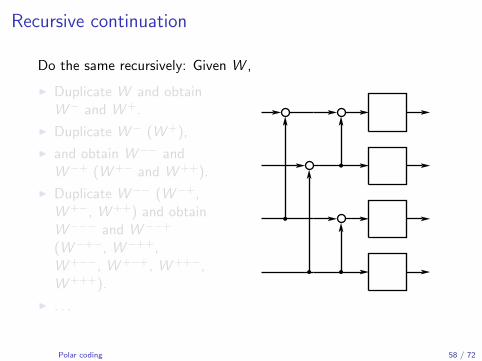
Recursive continuation
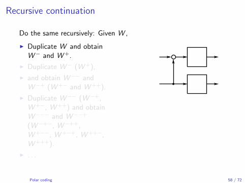
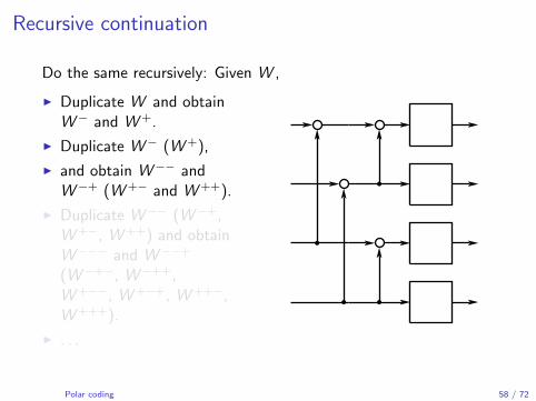
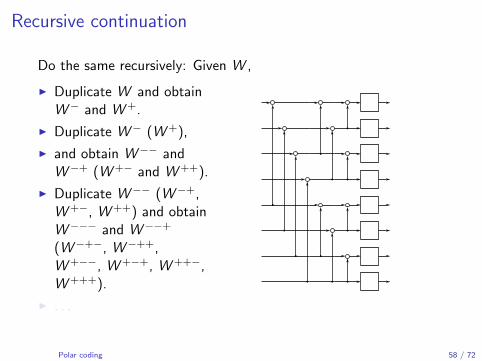
Do the same recursively: Given W ,
I Duplicate W and obtainW− and W+.
I Duplicate W− (W+),
I and obtain W−− andW−+ (W+− and W++).
I Duplicate W−− (W−+,W+−, W++) and obtainW−−− and W−−+
(W−+−, W−++,W+−−, W+−+, W++−,W+++).
I . . .
Polar coding 58 / 72
Recursive continuation
Do the same recursively: Given W ,
I Duplicate W and obtainW− and W+.
I Duplicate W− (W+),
I and obtain W−− andW−+ (W+− and W++).
I Duplicate W−− (W−+,W+−, W++) and obtainW−−− and W−−+
(W−+−, W−++,W+−−, W+−+, W++−,W+++).
I . . .
Polar coding 58 / 72

Recursive continuation
Do the same recursively: Given W ,
I Duplicate W and obtainW− and W+.
I Duplicate W− (W+),
I and obtain W−− andW−+ (W+− and W++).
I Duplicate W−− (W−+,W+−, W++) and obtainW−−− and W−−+
(W−+−, W−++,W+−−, W+−+, W++−,W+++).
I . . .
Polar coding 58 / 72
Recursive continuation
Do the same recursively: Given W ,
I Duplicate W and obtainW− and W+.
I Duplicate W− (W+),
I and obtain W−− andW−+ (W+− and W++).
I Duplicate W−− (W−+,W+−, W++) and obtainW−−− and W−−+
(W−+−, W−++,W+−−, W+−+, W++−,W+++).
I . . .
Polar coding 58 / 72
Recursive continuation
Do the same recursively: Given W ,
I Duplicate W and obtainW− and W+.
I Duplicate W− (W+),
I and obtain W−− andW−+ (W+− and W++).
I Duplicate W−− (W−+,W+−, W++) and obtainW−−− and W−−+
(W−+−, W−++,W+−−, W+−+, W++−,W+++).
I . . .
Polar coding 58 / 72

Recursive continuation
Do the same recursively: Given W ,
I Duplicate W and obtainW− and W+.
I Duplicate W− (W+),
I and obtain W−− andW−+ (W+− and W++).
I Duplicate W−− (W−+,W+−, W++) and obtainW−−− and W−−+
(W−+−, W−++,W+−−, W+−+, W++−,W+++).
I . . .
Polar coding 58 / 72

Polarization ProcessEvolution of I = I (W ), I+ = I (W+), I− = I (W−), etc.
0
1
I
Polar coding 59 / 72
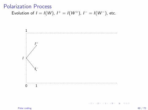
Polarization ProcessEvolution of I = I (W ), I+ = I (W+), I− = I (W−), etc.
0
1
1
I
I+
I−
Polar coding 60 / 72

Polarization ProcessEvolution of I = I (W ), I+ = I (W+), I− = I (W−), etc.
0
1
1 22
I
I+
I−
I++
I−+
I+−
I−−
Polar coding 61 / 72

Polarization ProcessEvolution of I = I (W ), I+ = I (W+), I− = I (W−), etc.
0
1
1 22 3333
I
I+
I−
I++
I−+
I+−
I−−
Polar coding 62 / 72

Polarization ProcessEvolution of I = I (W ), I+ = I (W+), I− = I (W−), etc.
0
1
1 22 3333 44444444
I
I+
I−
I++
I−+
I+−
I−−
Polar coding 63 / 72

Polarization ProcessEvolution of I = I (W ), I+ = I (W+), I− = I (W−), etc.
0
1
1 22 3333 44444444 5555555555555555
I
I+
I−
I++
I−+
I+−
I−−
Polar coding 64 / 72

Polarization ProcessEvolution of I = I (W ), I+ = I (W+), I− = I (W−), etc.
0
1
1 22 3333 44444444 5555555555555555 66666666666666666666666666666666
I
I+
I−
I++
I−+
I+−
I−−
Polar coding 65 / 72

Polarization ProcessEvolution of I = I (W ), I+ = I (W+), I− = I (W−), etc.
0
1
1 22 3333 44444444 5555555555555555 66666666666666666666666666666666 7777777777777777777777777777777777777777777777777777777777777777
I
I+
I−
I++
I−+
I+−
I−−
Polar coding 66 / 72

Polarization ProcessEvolution of I = I (W ), I+ = I (W+), I− = I (W−), etc.
0
1
1 22 3333 44444444 5555555555555555 66666666666666666666666666666666 7777777777777777777777777777777777777777777777777777777777777777 88888888888888888888888888888888888888888888888888888888888888888888888888888888888888888888888888888888888888888888888888888888
I
I+
I−
I++
I−+
I+−
I−−
Polar coding 67 / 72

Cutoff Rate Polarization
Theorem (2006)
The cutoff rates {R0(Ui ;YNU i−1)} of the channels created by the
recursive transformation converge to their extremal values, i.e.,
1
N#{i : R0(Ui ;Y
NU i−1) ≈ 1}→ I (W )
and1
N#{i : R0(Ui ;Y
NU i−1) ≈ 0}→ 1− I (W ).
Remark: {I (Ui ;YNU i−1)} also polarize.
Polar coding 68 / 72

Sequential decoding with successive cancellation
I Use the recursive construction to generate N bit-channelswith cutoff rates R0(Ui ;Y
NU i−1), 1 ≤ i ≤ N.
I Encode the bit-channels independently using convolutionalcoding
I Decode the bit-channels one by one using sequential decodingand successive cancellation
I Achievable sum cutoff rate is
N∑i=1
R0(Ui ;YNU i−1)
which approaches N I (W ) as N increases.
Polar coding 69 / 72

Final step: Doing away with sequential decoding
I Due to polarization, rate loss is negligible if one does not usethe “bad” bit-channels
I Rate of polarization is strong enough that a vanishing frameerror rate can be achieved even if the “good” bit-channels areused uncoded
I The resulting system has no convolutional encoding andsequential decoding, only successive cancellation decoding
Polar coding 70 / 72

Polar coding
To communicate at rate R < I (W ):
I Pick N, and K = NR good indices i such that I (Ui ;YNU i−1)
is high,
I let the transmitter set Ui to be uncoded binary data for goodindices, and set Ui to random but publicly known values forthe rest,
I let the receiver decode the Ui successively: U1 from Y N ; Ui
from Y N U i−1.
Polar coding 71 / 72

Polar coding complexity and performance
Theorem (2007)
With the particular one-to-one mapping described here and withthe successive cancellation decoding, polar codes achieve thecapacity I (W ) with
I encoding complexity N logN,
I decoding complexity N logN,
I and probability of frame error better than 2−N0.49
Polar coding 72 / 72

Next lecture
I Details of the construction, encoding and decoding algorithms
I Survey of important results about polar codes
I Potential for applications
Polar coding 73 / 72

Next lecture
I Details of the construction, encoding and decoding algorithms
I Survey of important results about polar codes
I Potential for applications
Polar coding 73 / 72

Next lecture
I Details of the construction, encoding and decoding algorithms
I Survey of important results about polar codes
I Potential for applications
Polar coding 73 / 72

Thank you!
Polar coding 74 / 72