Polar Fourier transforms of radially sampled NMR data · Polar Fourier transforms of radially sampled NMR data Brian E. Coggins, ... analysis of the discrete polar Fourier transform,

www.elsevier.com/locate/jmr

Journal of Magnetic Resonance 182 (2006) 84–95

Polar Fourier transforms of radially sampled NMR data

Brian E. Coggins, Pei Zhou *

Department of Biochemistry, Duke University Medical Center, Durham, NC 27710, USA

Received 5 April 2006; revised 2 June 2006Available online 3 July 2006

Abstract

Radial sampling of the NMR time domain has recently been introduced to speed up data collection significantly. Here, we show thatradially sampled data can be processed directly using Fourier transforms in polar coordinates. We present a comprehensive theoreticalanalysis of the discrete polar Fourier transform, and derive the consequences of its application to radially sampled data using linearresponse theory. With adequate sampling, the resulting spectrum using a polar Fourier transform is indistinguishable from convention-ally processed spectra with Cartesian sampling. In the case of undersampling in azimuth—the condition that provides significant savingsin measurement time—the correct spectrum is still produced, but with limited distortion of the baseline away from the peaks, taking theform of a summation of high-order Bessel functions. Finally, we describe an intrinsic connection between the polar Fourier transformand the filtered backprojection method that has recently been introduced to process projection-reconstruction NOESY data. Direct polarFourier transformation holds great potential for producing quantitatively accurate spectra from radially sampled NMR data.� 2006 Elsevier Inc. All rights reserved.

Keywords: Polar Fourier transform; Radial sampling

1. Introduction

In recent years, a number of multidimensional NMRtechniques have been proposed that share in common thesampling of the time domain along radial spokes [1–16],an approach that has been termed radial sampling [17].The conventional procedure for multidimensional experi-ments, which consists of sampling the time domain on aCartesian grid, requires measurement times that canbecome significant for the three- or more dimensionalexperiments that constitute the foundation of modern bio-molecular NMR. The drive for increased throughput instudies of small biomolecules, as well as the demand forexperiments with more dimensions and higher resolutionin studies of large biomolecules, have together motivatedthe exploration of alternative approaches.

Sampling the time domain along radial spokes is synon-ymous with coevolving two or more indirect dimensions of

1090-7807/$ - see front matter � 2006 Elsevier Inc. All rights reserved.

doi:10.1016/j.jmr.2006.06.016

* Corresponding author. Fax: +1 919 684 8885.E-mail address: [email protected] (P. Zhou).

an experiment, a procedure related to the historical accor-

dion spectroscopy [2], and which has become commonrecently in the form of the reduced dimensionality (RD)experiments and their more recently introduced cousins,the GFT experiments [3–7,11,18]. Customarily, these RD/GFT experiments would measure a single radial slice alongthe diagonal of the time domain, which would be Fouriertransformed to give a lower dimensional spectrum, withpeak positions determined as linear combinations of thefrequencies in the jointly sampled dimensions. The projec-

tion spectroscopy methods develop this sampling further,by measuring multiple radial slices of the time domain, atdifferent angles, which are each Fourier transformed inde-pendently to yield a set of projection spectra [8–10,12–16].The projection interpretation is a powerful one, and haslead to a variety of methods for utilizing the radiallysampled data, which can be classified into those thatcompute reconstructions of the full higher-dimensionalspectrum from the lower-dimensional projections[8–10,12,13,16,19], and those that analyze the peak posi-tions on the projections directly [14,15,20].

mailto:[email protected]

B.E. Coggins, P. Zhou / Journal of Magnetic Resonance 182 (2006) 84–95 85

An interesting question is whether radially sampledNMR data could be processed directly with a multidimen-sional Fourier transform (FT), yielding a quantitative high-er-dimensional spectrum determined according to thefamiliar properties of the FT. Noting that the samplingprocedure used in the projection spectroscopy method isessentially a sampling in polar coordinates, we turned toforms of the discrete FT that operate in a polar domain,which we refer to collectively as the polar FT (PFT). Here,we evaluate the unique properties of the polar FT, and con-sider in detail its application to radially sampled NMRdata.

When our study was completed, we learned of a paralleleffort by Kazimierczuk and coworkers, now recently pub-lished [21], involving the computation of spectra from bothradially and spirally-sampled data, using the traditionalequation for the discrete FT (DFT). Our work has focusedspecifically on the radial case, to obtain a comprehensiveunderstanding of its qualities. Additionally, our PFT equa-tions point to an oversight in the previous DFT work:There is a need to correct for the unequal area density ofthe sampling pattern, in order to obtain quantitative peaklineshapes.

In this article, we derive analytical expressions govern-ing the spectra obtained for discrete NMR data, providinga theoretical understanding of the numerical and experi-mental results reported previously for the radial case. Animportant result is the determination that it is possible toobtain spectra that are virtually identical to those generat-ed by discrete FTs of data sampled on Cartesian grids. Wefurther discuss a connection between polar Fourier trans-forms and the filtered backprojection method for quantita-tive reconstruction from projections.

2. Theory

2.1. Notation

Throughout this paper, lower-case variables representfunctions and coordinates in the NMR time domain, whileupper-case letters represent the same for the NMR fre-quency domain. We denote a Fourier transform pair usinga double-headed arrow

f ðxÞ () F ðX Þ: ð1Þ

Convolution is indicated with an asterisk,

f ðxÞ � gðxÞ �Z 1

�1f ðuÞgðx� uÞdu; ð2Þ

which is readily extended to multiple dimensions. The func-tion P (x) is the rectangular cutoff

PðxÞ �1 jxj < 1=2;

1=2 jxj ¼ 1=2;

0 jxj > 1=2:

8><>: ð3Þ

Its Fourier transform is the sinc function, defined to be

sinc x � sin pxpx

: ð4Þ

The function d2-D (x,y) represents the Dirac delta functionin 2-D

d2-Dðx; yÞ �1 x; y ¼ 0;

0 x or y 6¼ 0:

�ð5Þ

We follow Bracewell [22] in using d2-D of a single variableto designate a delta function dependent only on the onevariable, that is, a line impulse. For example

d2-DðxÞ ¼1 x ¼ 0;

0 x 6¼ 0

�ð6Þ

describes an infinitely sharp impulse along the y-axis. Thedirection of an impulse d2-D (u) is always normal to thedirection described by u. Note also that d2-D (x,y) =d2-D (x)d2-D (y).

An infinite 1-D train of impulses spaced at integer incre-ments in x is the pulse train function III

IIIðxÞ �X1

i¼�1dðx� iÞ: ð7Þ

In discussions of delta functions and other functionsthat do not have conventional integrals, the generalizedfunction interpretation of an integral in the limit isassumed [22,23].

2.2. Continuous radial polar transforms

The starting point for our discussions will be the con-ventional Cartesian Fourier transform of a continuous 2-D complex-valued function f (x,y)

F ðX ; Y Þ ¼Z 1

�1

Z 1

�1f ðx; yÞe�2piðxXþyY Þ dxdy: ð8Þ

One approach to calculate a spectrum would be to evaluatethis equation directly for the known sampling points, withthe rest of the domain implicitly assumed to be zero [21].This could be used for radial data. However, it is reason-able to ask whether changing Eq. (8) to polar coordinateswould give additional insight into the situation.

Substituting r ¼ffiffiffiffiffiffiffiffiffiffiffiffiffiffix2 þ y2

pand h = arctan y/x, and

changing the differentials dxdy to rdrdh, Eq. (8) becomesthe continuous transform of a radially sampled function[24,25]:

F ðX ; Y Þ ¼Z 2p

0

Z 1

0

f ðr; hÞe�2pirðX cos hþY cos hÞr dr dh; ð9Þ

where 0 6 h < 2p and 0 6 r <1.The primary difference between Eqs. (9) and (8) is the

factor r in the change of differentials, which corrects forthe unequal area density of sampling points in the radialpattern. Without this correction, each infinitesimal areaelement defined by drdh would be given uniform weight-ing, even though the sizes of these elements are not uniformover the whole plane. This has more general implications

86 B.E. Coggins, P. Zhou / Journal of Magnetic Resonance 182 (2006) 84–95

for FT processing of data sampled on non-Cartesian pat-terns, which we will discuss in detail below.

The fact that we represent F in Cartesian coordinates inEq. (9), despite changing f to polar coordinates, is worthyof comment. Although it is possible to calculate F in apolar space, it is important to recognize that the Fouriertransform always produces equal information about F forall points in the X/Y plane, regardless of the coordinatesystem of the input function f. We conclude that the evenlydistributed Cartesian grid is better suited than a polar gridfor reporting the transform results.

As written in Eq. (9), the transform is evaluated first withrespect to r, and second with respect to h. We shall refer tothis form of the polar FT as a radial transform. This equationfits naturally with the interpretation of the 2-D FT kernel as asuperposition of 1-D cosine and sine waves in all directions[22,26]; here, each spoke of f (r,h) at fixed h contributes theweighting coefficients for the cosine and sine waves in direc-tion h used in the synthesis of F (Fig. 1). Since the specificposition along a kernel wave in direction h for a pointF (X,Y) can be located with a frequency domain radial coor-dinate R 0 = Xcosh + Ycosh, we can write

RadialRadiala b

Fig. 1. Radial form of the polar FT. (a) In the radial form, the transform is cofrom waves in all directions and of all radial frequencies. The amplitude of a sin(blue point in a), with the frequency determined by the distance of the point f

Azimuthala b

Fig. 2. Azimuthal form of the polar FT. (a) In the azimuthal form, the transfperiod n about the ring and the data f determines the weighting coefficient focontour plot with positive contours in blue and negative contours in red, vari

F ðX ; Y Þ ¼Z 2p

0

Z 1

0

f ðr; hÞe�2pirR0r dr dh ð10Þ

showing that the innermost integration is essentially a 1-DFT with respect to r. Letting Fr represent the data follow-ing this integration, we find that Fr is entirely in the fre-quency domain, and that the kernel has been evaluatedcompletely. All that remains is a simple integration of Fr

along h. This is in contrast to the standard Cartesian ap-proach of separating the kernel into x and y components,where following transformation over one variable, the ker-nel component for the other variable still remains.

2.3. Continuous azimuthal polar transforms

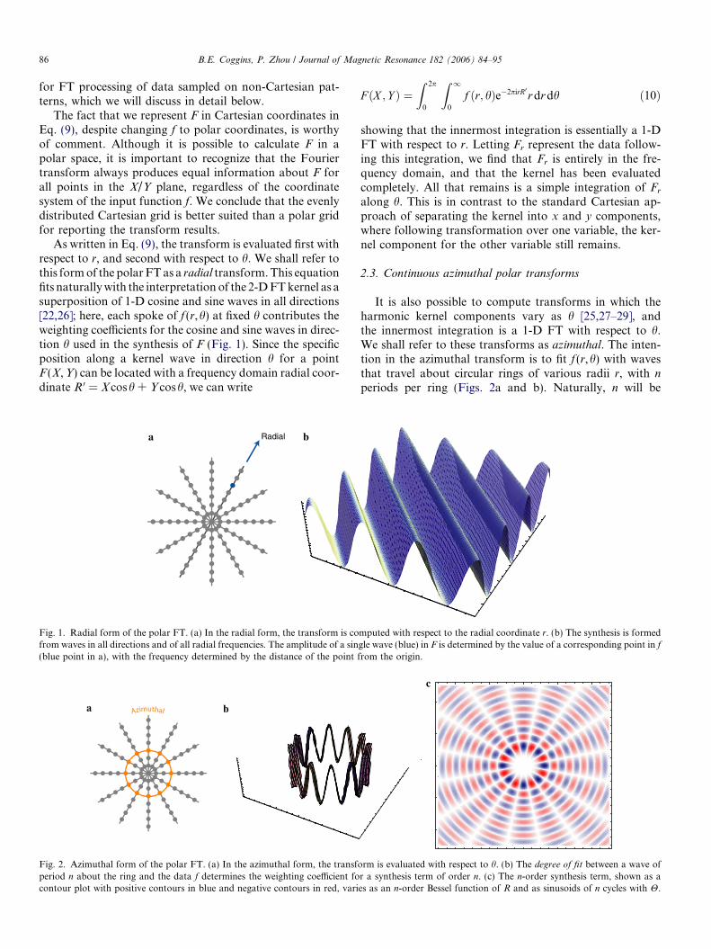
It is also possible to compute transforms in which theharmonic kernel components vary as h [25,27–29], andthe innermost integration is a 1-D FT with respect to h.We shall refer to these transforms as azimuthal. The inten-tion in the azimuthal transform is to fit f (r,h) with wavesthat travel about circular rings of various radii r, with n

periods per ring (Figs. 2a and b). Naturally, n will be

mputed with respect to the radial coordinate r. (b) The synthesis is formedgle wave (blue) in F is determined by the value of a corresponding point in f

rom the origin.

c

orm is evaluated with respect to h. (b) The degree of fit between a wave ofr a synthesis term of order n. (c) The n-order synthesis term, shown as aes as an n-order Bessel function of R and as sinusoids of n cycles with H.


limited to integers. Eq. (9) can be rearranged so that theinnermost integration is over h

F ðX ; Y Þ ¼Z 1

0

Z 2p

0

f ðr; hÞe�2pirðX cos hþY sin hÞr dhdr

¼Z 1

0

Z 2p

0

f ðr; hÞe�2pirðR cos H cos hþR sin H sin hÞr dhdr

¼Z 1

0

Z 2p

0

f ðr; hÞe�2pirR cosðh�HÞr dhdr; ð11Þ

where we introduce R ¼ffiffiffiffiffiffiffiffiffiffiffiffiffiffiffiffiffiX 2 þ Y 2

pand H = arctanY/X.

Using the following relation [29]:

eiu cos / ¼X1

n¼�1inJ nðuÞein/; ð12Þ

where Jn is the Bessel function of order n, taking u = 2prR

and / = h � H, we derive

F ðX ; Y Þ ¼Z 1

0

Z 2p

0

X1n¼�1

f ðr; hÞinJ nð2prRÞeinðH�hÞr dh dr:

ð13Þ

Eq. (13) can be rearranged as

F ðX ; Y Þ ¼Z 1

0

X1n¼�1

Z 2p

0

f ðr; hÞe�inh dh

� �inJ nð2prRÞeinHr dr:

ð14Þ

The integral in brackets is a 1-D Fourier transformwith respect to h. This transform over h explicitly ana-lyzes f into harmonic components of h, indexed by theirinteger angular frequencies n (Fig. 2b). The amplitudesof the harmonic components in this transform provideweighting coefficients for the components used in thefinal synthesis of F, which vary with H as sinusoidsand with R as Bessel functions of various orders. Anexample of one of these components is plotted inFig. 2c.

The azimuthal and radial transforms are equivalentmethods for calculating the continuous polar 2-D Fouriertransform. For practical NMR signal processing, it isadvantageous to adopt the radial transform, as it can beevaluated as a 1-D transform with respect to r followedby an integration, while the azimuthal involves a 1-Dtransform with respect to h followed by the summationof a series of Bessel function terms. Additionally, the radi-al transform can be conveniently extended to hyperdimen-sional spaces, simply by changing the weighting factor r

and integrating over the additional angles. However,extending the azimuthal transforms to higher-dimensionalfunctions requires introducing spherical or even higher-di-mensional polar harmonics. Nevertheless, we find the azi-muthal transform to be a useful analytical tool forpredicting the consequences of limited sampling in the azi-muthal coordinate for 2-D functions.

2.4. NMR data and discrete transforms

Several additional considerations must be addressedbefore the calculation of spectra from NMR data arepossible using the above equations. First, the multidi-mensional NMR time domain is normally observed ashypercomplex rather than complex data, i.e., lettingfx (x) and fy (y) represent the signals arising from theevolution of nuclei in x and y, respectively, fourhypercomplex observations are made:

I1ðr; hÞ ¼ Re½fxðr cos hÞ�Re½fyðr sin hÞ�;I2ðr; hÞ ¼ Re½fxðr cos hÞ�Im½fyðr sin hÞ�;I3ðr; hÞ ¼ Im½fxðr cos hÞ�Re½fyðr sin hÞ�;I4ðr; hÞ ¼ Im½fxðr cos hÞ�Im½fyðr sin hÞ�;

ð15Þ

rather than the two complex components Re [f (r,h)]and Im[f (r,h)] needed in Eq. (9). By inserting a factor i

for each imaginary component measured, we obtain thedesired complex data as a linear combination of theobservations:

f ðr; hÞ ¼ 1

2ðRe½fxðr cos hÞ�Re½fyðr sin hÞ�

� Im½fxðr cos hÞ�Im½fyðr sin hÞ�Þ

þ i2ðRe½fxðr cos hÞ�Im½fyðr sin hÞ�

þ Im½fxðr cos hÞ�Re½fyðr sin hÞ�Þ

¼ 1

2ðI1 � I4Þ þ

i2ðI2 þ I3Þ: ð16Þ

NMR signals are causal, meaning that observations canonly be made for the +x +y quadrant, corresponding topositive evolution times. The Fourier transformation of acomplex dataset populated only for the +x +y quad-rant—as generated by Eq. (16)—leads to mixed-phase or‘‘phase-twist’’ lineshapes, due to the superposition of dis-persive and absorptive components [30]

Re½F þxþyðX ; Y Þ� ¼ Re½Fx�Re½Fy � � Im½Fx�Im½Fy �; ð17Þ

In order to obtain purely absorptive lineshapes, we em-ploy a mirror-image reflection of the +x +y data intothe �x +y quadrant, while taking the complex conjugatewith respect to x. This procedure is closely related to thetime-reversal method used historically in 2D J spectros-copy [30]. The reflection is computed using the linearcombination

f ðr; p� hÞ ¼ 1

2ðRe½fxðr cos hÞ�Re½fyðr sin hÞ�

þ Im½fxðr cos hÞ�Im½fyðr sin hÞ�Þ

þ i2ðRe½fxðr cos hÞ�Im½fyðr sin hÞ�

� Im½fxðr cos hÞ�Re½fyðr sin hÞ�Þ

¼ 1

2ðI1 þ I4Þ þ

i2ðI2 � I3Þ: ð18Þ


Since �gð�uÞ () GðUÞ, the transform of the reflected �x

+y data alone also has a phase-twist shape, but with thesigns of the phase-twist lobes reversed

Re½F �xþyðX ; Y Þ� ¼ Re½Fx�Re½Fy � þ Im½Fx�Im½Fy �: ð19ÞCombining the original data (Eq. (16)) and the reflecteddata (Eq. (18)) and computing the FT, the dispersivecomponents cancel, and a purely absorptive lineshape isobtained. The �y half of the time domain is left at zero topreserve causality in the final transform, ensuring thatIm[F (X,Y)] is the Hilbert transform of Re [F (X,Y)] andmay be discarded, as with conventional spectra [31].Thediscrete transform could be calculated at this point by directevaluation of Eq. (9) or (10), but it is computationallymore efficient to calculate the inner integral as a 1-D FFTwith respect to r. The limits of Eq. (10) are first changed

F ðX ; Y Þ ¼Z p

0

Z 1

�1f ðr; hÞe�2pirR0 jrjdr dh; ð20Þ

so that each radial spoke includes negative r evolutiontimes, corresponding to the �y half of the plane, suppliedin practice by twofold zero filling along each radial vector.After computing the FFT for spokes in directions0 6 h 6 p, one has an intermediate dataset Fr, sampledfor discrete positions of the R 0 coordinate. The final sum-mation over h requires interpolation to a Cartesian grid,carried out here as previously described for PR purposes[32]. The proper resolution for the discrete X/Y grid isdetermined by the maximum evolution time rmax.

2.5. Point response functions

Having defined the forms of the polar transform, wenow consider the behavior of this transform for discretedata. Linear response theory, which was used extensivelyin the development of pulsed NMR, provides a powerfulframework for understanding the consequences of any dis-crete sampling method [22,23,30]. We are interested incharacterizing how the spectrum produced by a transformof discrete radially sampled data differs from the true spec-trum of the continuous signal.

Discrete sampling methods can be treated as linear sys-tems that operate on a theoretically continuous input toyield the actual, observed output [22,24,25]

F WðX ; Y Þ ¼ W½F ðX ; Y Þ�; ð21Þ

where W represents the action of the sampling filter to gen-erate the output spectrum FW from a signal with true spec-trum F. The result of W can be determined for any input ifwe know the characteristic point response of W

HWðX ; Y Þ ¼ W½d2-DðX ; Y Þ�; ð22Þwhich is the response to an input that is an infinitely sharppoint signal [22,23,25,30]. The point response is oftencalled the ‘‘point-spread function,’’ because it describeshow the process W spreads the infinitely sharp point intoa finite image. The foundation of response theory is that

if the impulse response is known, the output of the systemcan be calculated for any arbitrary input [22,23,30]

F WðX ; Y Þ ¼ F ðX ; Y Þ � HWðX ; Y Þ: ð23Þ

While our goal is to understand the effects of the sam-pling process on the final result in the frequency domain,the actual sampling for NMR happens in the time domain.The sampling process is equivalent to multiplying the con-tinuous signal by a sampling function s (r,h), which is onefor any value that is sampled, and zero otherwise, and thentaking the (continuous) Fourier transform:

W½F ðX ; Y Þ� �Z p

0

Z 1

�1f ðr; hÞsðr; hÞe�2pirR0 jrjdr dh: ð24Þ

The point response HW is then:

HWðX ; Y Þ ¼ W½d2-DðX ; Y Þ�

¼Z p

0

Z 1

�1sðr; hÞe�2pirR0 jrjdr dh ¼ SðX ; Y Þ; ð25Þ

where we have used the Fourier transform paird2-DðX ; Y Þ () 1. Thus the point response function HW isnothing more than the transform S (X,Y) of the samplingfunction s, indicating that it is in fact the sampling patternthat directly determines the manner and extent of variationfrom the true spectrum.

2.6. Point response functions for discrete sampling in

azimuth

We now consider the effects of discrete radial sampling,by defining a suitable s and computing its FT. The mostsalient characteristic of the NMR sampling pattern as prac-ticed to date is limited sampling in h. This characteristic haspermitted the enormous time savings over conventionalsampling, and it is the consequences of this limited sam-pling that are most important for assessing the results ofFourier transforming this data into a spectrum. By com-parison, the sampling in r is on par with conventionalapproaches, and its discreteness should have much lessimpact on the result.

Given these facts, it is thus interesting to consider a sam-pling function sN which is discrete in h, but continuous in r.This function can be defined in Cartesian and polar coordi-nates as:

sN ðx; yÞ ¼XN

i¼1

d2-Dðx sin ui þ y cos uiÞ;

sN ðr; hÞ ¼XN

i¼1

d2-Dðr cos h sin ui þ r sin h cos uiÞ; ð26Þ

where N radial spokes are measured for directions from 0to p (i.e., following processing by Eqs. (16) and (18)), theazimuth value for a given spoke i denoted as ui. It is as-sumed that the spokes are distributed evenly in h. The radi-al PFT of this sampling function is then


SN ðX ; Y Þ ¼XN

i¼1

Z 1

�1d2-Dðr cos h sin ui

þ r sin h cos uiÞe�2pirR0 jrjdr: ð27Þ

It is convenient to represent this transform as the summa-tion of an intermediate result

SN ðX ; Y Þ ¼XN

i¼1

SN ;rðR0; hÞ; ð28Þ

where SN,r can be written, using the convolution theoremand the FT pair d2-DðxÞ () d2-DðY Þ [22], as

SN ;rðR0; hÞ ¼ d2-DðR0 cos h sinðui þp2Þ þ R0 sin h cosðui þ

p2ÞÞ

�Z 1

�1jrje�2pirR0 dr: ð29Þ

However, the transformation of the weighting function |r|at the end of Eq. (29) poses a problem, as it does not con-verge. To resolve this, Eq. (29) must be modified to imposea cutoff on r of rmax, beyond which r = 0 [24,25,33]. Usingthe rectangular cutoff P of Eq. (3), the latter integral thenbecomesZ 1

�1P

r2rmax

� �jrje�2pirR0 dr ¼ 2rmax sinc 2 rmaxR0

� rmaxsinc2 rmaxR0; ð30Þ

and the frequency domain intermediate result follows:

SN ;rðR0;hÞ¼ d2-D R0 coshsin uiþp2

� þR0 sinhcos uiþ

p2

� � � ð2rmax sinc 2rmaxR0 � rmax sinc2 rmaxR0Þ:

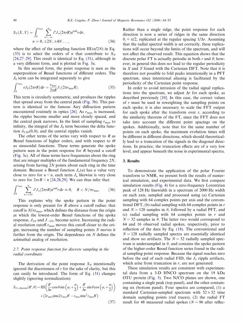
ð31ÞA numerical simulation of the point response for N = 25

is plotted in Fig. 3a. The point response that we havederived is the superposition of a contribution for each

Fig. 3. Point response functions for discrete radial sampling. (a) The point respoint response, which becomes J1 following integration. This term arises fromgenerated by the higher-order terms of the point response (here, for N = 25). Thpredicted analytically. This is the observed pattern of artifacts for a signal tha

radial spoke. A radial spoke in direction hi contributes aset of ridges in the direction hi + p/2, with the overall shapedefined by Eq. (30). As one might expect, increasing thecutoff rmax, representing an increase in the radial resolu-tion, leads to a sharpening of the contribution in each sam-pled direction; in the limit of infinite r, the point responsebecomes the superposition of line impulses normal to thetime domain sampling directions. The final pattern couldbe described in a simplified way as an ‘‘aster’’ or ‘‘star’’ pat-tern with N spokes, but this does not take into accountmany details of the response, including the disappearanceof the spokes, and their replacement by symmetric ripples,for R coordinates below a cutoff.

It is perhaps more informative to consider an alternativeformulation of the point response. Instead of treating s asthe sum of N continuous spokes cut off at rmax, we canconsider s to be the integration for radii up to rmax of ringswith radius r 0 each sampled N times over the range of 0 to p

sNðr; hÞ ¼Z rmax

0

dðr � r0ÞðN=pÞIIIðhN=pÞdr0: ð32Þ

The cutoff at rmax is required for the same reason as therectangular cutoff in Eq. (30), so that integration of theweighting factor r in a polar FT will converge. The azi-muthal FT of this function is then calculated by first takinga 1-D transform with respect to h for a given radius r

(Fig. 2) [29]:

SN ;hðr; nÞ ¼Z 2p

0

ðN=pÞIIIðhN=pÞe�inhdh ¼ 2NIIIðn=2NÞ:

ð33ÞThe transform III (n/2N) indicates that the 2N delta func-tions per ring of the sampling function can be synthesizedfrom a series of waves around the ring, with frequenciesthat are integer multiples of the fundamental frequency2N. This can then be substituted into Eq. (14) to give

ponse function SN for N = 25. (b) The circularly symmetric J0 term of thetruncation of the signal in the radial dimension r. (c) The spoke pattern

is spoke pattern contains a clear zone without artifacts, the size of which ist is not truncated in r.


SN ðX ; Y Þ ¼Z rmax

0

X1n¼�1

inJ nð2prRÞeinHr dr;

n ¼ 0;�2N ;�4N . . . ; ð34Þ

where the effect of the sampling function III (n/2N) in Eq.(33) is to select the orders of n that contribute to SN

[24,27–29]. This result is identical to Eq. (31), although ina very different form, and is plotted in Fig. 3a.

In this second form, the point response is seen as thesuperposition of Bessel functions of different orders. TheJ0 term can be integrated separately to giveZ rmax

0

rJ 0ð2prRÞdr ¼ rmax

2pRJ 1ð2prmaxRÞ: ð35Þ

This term is circularly symmetric, and produces the ripplesthat spread away from the central peak (Fig. 3b). This pat-tern is identical to the famous Airy diffraction patternencountered routinely in optics [26]. As rmax is increased,the ripples become smaller and more closely spaced, andthe central peak narrows. In the limit of sampling rmax toinfinity, the integral of the J0 term becomes the delta func-tion d2-D (0,0), and the central ripples vanish.

The other terms of the series vary with respect to R asBessel functions of higher orders, and with respect to Has sinusoidal functions. These terms generate the spokepattern seen in the point response for R beyond a cutoff(Fig. 3c). All of these terms have frequencies about the ringthat are integer multiples of the fundamental frequency 2N,arising from having 2N points about each ring in the timedomain. Because a Bessel function Jn (u) has a value veryclose to zero for u < n, each term Jn likewise is very closeto zero for 2prR < n [24,28,29]. We can thus infer that:Z rmax

0

X1n¼�2N

inJ nð2prRÞeinHr dr � 0; R < N=prmax: ð36Þ

This explains why the spoke pattern in the pointresponse is only present for R above a cutoff radius: thatcutoff is N/prmax, which defines the distance from the originat which the lowest-order Bessel functions of the spokeresponse, J2N and J�2N, become active. Increasing the radi-al resolution cutoff rmax moves this cutoff closer to the ori-gin; increasing the number of sampling points N moves itfarther from the origin. The dependence on N defines theazimuthal analog of resolution.

2.7. Point response function for discrete sampling in the

radial coordinate

The derivation of the point response SN intentionallyignored the discreteness of r for the sake of clarity, but thiscan easily be introduced. The form of Eq. (31) changesslightly (ignoring normalization):

SN ;r;discrete R0;hð Þ¼ IIIR0

Drcoshsin uiþ

p2

� þ R0

Drsinhcos uiþ

p2

� � �

� 2rmaxsinc2rmaxR0 � rmaxsinc2 rmaxR0 �

ð37Þ

Rather than a single ridge, the point response for eachdirection is now a series of ridges in the same directionhi + p/2, replicated at the regular spacing 1/Dr. Assumingthat the radial spectral width is set correctly, these replica-tions will occur beyond the limits of the spectrum, and willnot affect the observed result. This equation shows that thediscrete polar FT is actually periodic in both r and h; how-ever, in general this does not lead to the regular periodicityin X and Y found with the Cartesian DFT. Note that it istherefore not possible to fold peaks intentionally in a PFTspectrum, since intentional aliasing is facilitated by theperiodicity of the Cartesian point response.

In order to avoid intrusion of the radial signal replica-tions into the spectrum, we adjust Dr for each spoke, asdescribed previously [10]. In this case, the correct valuesof r must be used in reweighting the sampling points oneach spoke; it is also necessary to scale the FFT outputfor each spoke after the transform over r, according tothe similarity theorem of the FT, since the FFT does nottake into account the different point spacings on thespokes. Additionally, note that for the same number ofpoints on each spoke, the maximum evolution times willbe different in different directions, which should theoretical-ly lead to a truncation of the signals in the diagonal direc-tions. In practice, the truncation effects are of a very lowlevel, and appear beneath the noise in experimental spectra.

3. Results

To demonstrate the application of the polar Fouriertransform to NMR, we present both the results of numer-ical simulation, and experimental data. We first comparesimulation results (Fig. 4) for a zero-frequency Lorentzianpeak of 128 Hz linewidth in a spectrum of 2000 Hz widthon each axis, sampled and processed using (a) Cartesiansampling with 64 complex points per axis and the conven-tional DFT, (b) radial sampling with 64 complex points in r

and N = 128 samples in h, followed by a radial PFT, and(c) radial sampling with 64 complex points in r andN = 32 samples in h. The latter two would correspond to64 and 16 observed radial spokes, respectively, prior toreflection of the data by Eq. (18). The conventional andN = 128 radially sampled spectra are essentially identicaland show no artifacts. The N = 32 radially sampled spec-trum is undersampled in h, and contains the spoke patternof the higher-order Bessel function series found in the radi-al sampling point response. Because the signal reaches zerobefore the end of each radial FID, the J1 ripple artifacts,which arise from truncation in r, are not generated.

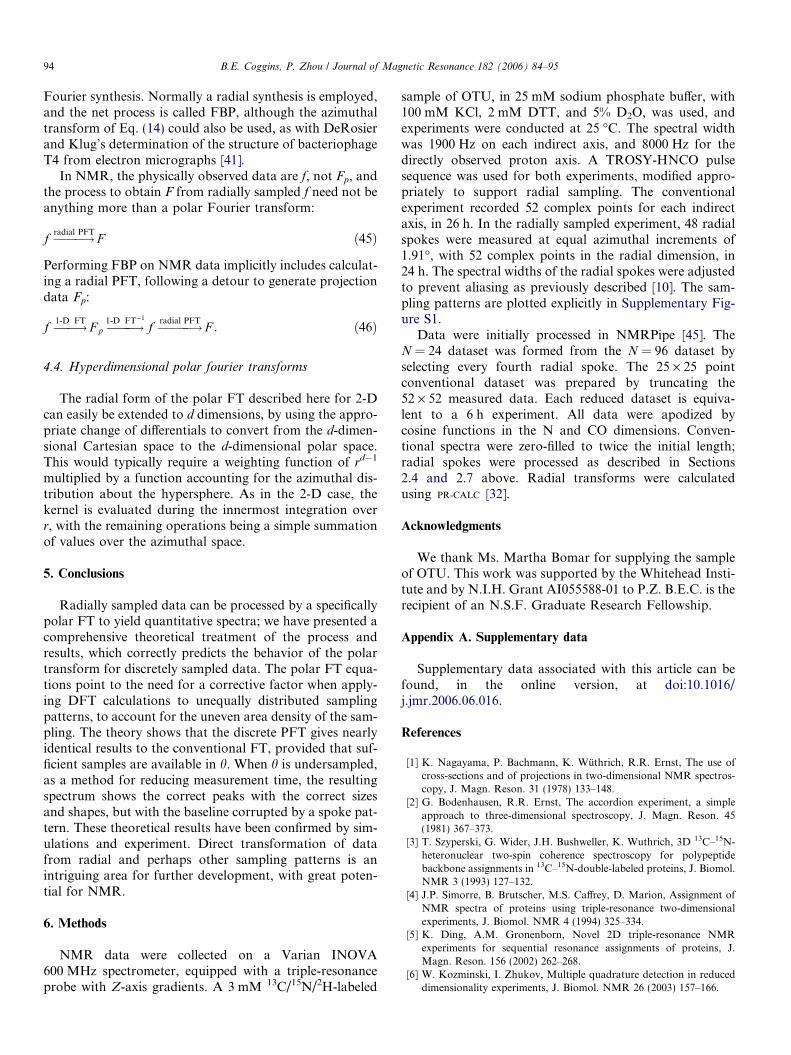
These simulation results are consistent with experimen-tal data from a 3-D HNCO spectrum on the 19 kDaOTU protein (Fig. 5). Two N/CO planes are shown, onecontaining a single peak (top panel), and the other contain-ing six (bottom panel). Four spectra are compared, (1) astandard Cartesian-sampled spectrum with 52 · 52 timedomain sampling points (red traces), (2) the radial FTresult for 48 measured radial spokes (N = 96 after reflec-

Fig. 4. Simulations of Cartesian and polar Fourier transforms. (a) The discrete Cartesian FT of a simulated Lorentzian peak. (b) The discrete radial polarFT of the same simulated Lorentzian peak, for N = 128 radial samples, each with 64 complex points in r. This transform correctly reproduces theLorentzian peak of (a), with a slight vertical offset due to the zeroing of the point at f (0,0) by the radial weighting function r, and with <0.1% baselinefluctuation due to limited numerical precision in the integration over h. (c) The discrete radial polar FT of the same peak, for N = 32 radial samples. Thespoke pattern arising from the higher-order Bessel terms in the point response is visible, extending almost to the base of the peak. The spokes are not ofidentical shape due to the convolution with the peak shape.


tion), each with 52 points (green traces), (3) the convention-al spectrum for 25 · 25 sampling points (purple traces) and(4) the radial FT spectrum for 12 radial spokes (N = 24after reflection) (blue traces). For clarity, the positions ofthe sampling points in the time domain for each datasethave been plotted in Supplementary Figure S1. These spec-tra compare Cartesian and radial results for two roughlyequal numbers of sampling points, (1) and (2) having2704 and 2496 points, respectively, and (3) and (4) having625 and 624 points, respectively. The right side of the figurefeatures N and CO 1-D cross-sections through some of thepeaks [(b) and (d)].

As with the simulation, the conventional 52 · 52 point and48 radial spoke results are essentially identical. The resultswith limited sampling show the consequences of the samplingpattern: The 625 point Cartesian spectrum has broadenedpeaks, while the peaks in the 12 radial spoke (N = 24)spectrum remain sharp, at the expense of picking up theJ48 Bessel spoke artifact pattern that is characteristic ofundersampling in h. This spoke pattern is of a low level bycomparison to the peaks, but is still quite significant. Thesensitivity in both �625 point spectra is reduced from thatof the�2500 point cases due to the decreased signal averaging.

The experimental and simulation results confirm theaccuracy of the theoretical predictions. We were able toreproduce the Cartesian results within the measurementerror, using radial sampling and polar transforms. In addi-tion, in cases of undersampling, both simulation and exper-iment reproduced the higher-order Bessel function pointresponse, as an artifact pattern corrupting the baseline awayfrom the peaks.

4. Discussion

4.1. Corrections for the area density of sampling points

The theoretical treatment of the polar FT leads to amore general conclusion about FT processing of data sam-

pled on non-Cartesian patterns. The proper conversion ofthe continuous FT (Eq. (8)) to a general discrete equationfor an arbitrary sampling pattern is

F DFTðX ; Y Þ ¼X

i

f xi; yið Þe�2piðxiXþyiY ÞDAi; ð38Þ

where a sampling point i at a position (xi,yi) has a weightDAi, reflecting the area it occupies in the x/y plane. In cons-trast with Kazimierczuk et al. [21], DAi may only be ig-nored for Cartesian sampling; in a general case it must bedetermined, ideally analytically, but if necessary by empir-ical methods such as the Voronoi diagram [34].

In the radial case, the proper weighting can be obtainedanalytically as DAi = riDrDh, which simplifies to ri as longas Dr and Dh are uniform (and in fact, when we vary Dr toprevent aliasing, as described above, an additional correc-tion must be made for the unequal Dr for different spokes).It has been shown for the FT processing of radiallysampled imaging data that computing the transformwithout this weighting factor leads to a convolutionbetween the true image (here, spectrum) and the function1/R [24]:

F uncorrectedðX ; Y Þ ¼ F ðX ; Y Þ � 1

R; ð39Þ

which results in a severe broadening of all peaks, dueto the overemphasis of low frequency components inthe synthesis of Funcorrected. For other unevenly distrib-uted sampling patterns, like the recently proposed spiralapproach [21], it will be important to determine theappropriate weighting factors to produce accurate peaklineshapes.

4.2. Lineshapes, artifacts, and time savings

Much of the recent interest in radial sampling has beendriven by the prospect of obtaining spectra in less measure-ment time than would be necessary with conventional

Fig. 5. Comparison of Cartesian and radial sampling for experimental data. Two N/CO planes from the 3-D HNCO spectrum of the 19 kDa OTU proteinare shown, at HN chemical shifts of 9.296 and 8.410 ppm for the top and bottom panels, respectively. Stacked plots are given for conventional Cartesian-sampled data with 2704 (52 · 52) or 625 (25 · 25) sampling points, processed by the conventional DFT, and for radially sampled data with 2496 (48spokes, 52 points each) or 624 points (12 spokes, 52 points each), processed by the radial form of the polar FT. At right are 1-D cross-sections in the N andCO directions passing through some of the peaks; the positions of the cross-sections are indicated by color-coded arrows on the stacked plots. Peakidentification in (d) is indicated with the symbols *, #, and %. (a) A plane containing a single peak. Full sampling produces essentially identical spectra,whether by the Cartesian or radial pattern. Undersampling of the conventional data leads to a loss of resolution, while undersampling of the radial dataresults in baseline artifacts assuming the spoke pattern of the J48 Bessel function. (b) Cross-sections through the same. (c) A plane containing six peaks. Allsix peaks are reproduced with the correct shapes and relative intensities in all spectra. (d) Cross-sections show accurate peak reproduction, but in theradially-undersampled case, there are also significant baseline artifacts.



methods. There has been some concern, however, aboutthe accuracy of spectra reconstructed from radialprojections.

The results of this study confirm analytically that it ispossible to obtain a quantitatively accurate spectrumfrom radially sampled data, if those data are processedusing a PFT, and if the degree of sampling is sufficient.Such spectra are equivalent to those obtained conven-tionally, within the error caused by noise and limitedprecision in the calculations. Because the method is anFT, the effects of relaxation and apodization on line-shapes is the same as with conventional data collection.Sensitivity is proportional to the number of measure-ments, since the same signal-averaging rules apply as inany FT. Two opposed factors influence the observed sen-sitivity: the increased sampling near the origin shouldincrease signal levels over Cartesian sampling with thesame number of data points, at least for decaying sig-nals; however, the reweighting of the data points in thepolar transform equation would counteract this. Theconsequences for the noise level and the resulting sig-nal-to-noise ratio are not entirely clear, and are an areafor further study.

We have also shown that it is possible to calculate aspectrum from a small number of radial samples, at theexpense of baseline artifacts following spoke patterns.The observed spectrum is a convolution between the truespectrum and the point response of the sampling process,with the consequence that the artifact pattern is replicatedfor each peak in the spectrum, centered on the peak, andscaled according to the size and shape of the peak. Withradial sampling, at a given resolution, there is a tradeoffbetween artifacts and measurement time, as dictated byEq. (36). While the artifacts may be problematic for exper-iments with a large dynamic range—such as NOESYexperiments with diagonal peaks—in cases where time isof the essence, accurate peak shapes are important, and alimited amount of artifacts are acceptable, a significant sav-ings in time may be realized by reducing the sampling in h,without leading to a loss of resolution. However, in theextreme of a very small number of radial spokes, the arti-facts will begin to overlap with the peaks, resulting in peakdistortion.

It should also be noted that since the sampling patterndirectly determines the artifact pattern (Eq. (23) or (25)),it might be possible to design other sampling patternswith a more favorable balance between artifacts, resolu-tion and measurement time. Spiral sampling is an exam-ple of a pattern that has been shown to generate reducedartifact levels by comparison with the radial approach[21]. However, it also important to ensure that any newpatterns reproduce peak shapes accurately, as we haveshown is the case for radial sampling. There is also greatpotential for the application of non-linear methods todeconvolute the artifact pattern [19]; the analytical under-standing of the artifact pattern given here may facilitatethis.

4.3. Connections to projection methods

There is a surprisingly close connection between thepolar FT and the filtered backprojection method describedin the literature. Consider the 1-D FT of a radial spoke in f

in a given direction h

F pðR; hÞ ¼Z 1

�1f ðr; hÞe�2pirR dr; ð40Þ

for 0 6 h < p and �1 < r <1. According to the projec-tion-slice theorem of the Fourier transform [1,22,35–37],Fp (R,h) is the projection of F at angle h, that is, the integra-tion of F along lines at angles h + p/2

F pðR; hÞ ¼Z 1

�1F R cos h� S sin h;R sin hþ S cos hð ÞdS:

ð41Þ

Many of the current efforts to determine NMR spectrafrom radially sampled data have focused on the idea ofinverting Eq. (41), to obtain F from Fp. A variety of meth-ods have been described for carrying out this inversion forNMR data [9,10,13,16,17,38,39], and even more methodshave been described in the literature of other scientific fields[24,25,28,33,35–37,40–44].

A popular method in the imaging community, whichwas recently demonstrated for NMR [13], is filtered back-

projection (FBP) [24,25,33,36,37,42,44]. FBP is the analyti-cal inversion of Eq. (41), and can be represented as:

F ðX ; Y Þ ¼Z p

0

Z 1

�1

Z 1

�1F P R0; hð Þe2pirR0dR0

� �

e�2pir X cos hþY cos hð Þjrjdr dh: ð42Þ

This method involves (1) inverse transformation of Fp,(2) filtering by a filter function |r|, (3) forward transforma-tion to give a ‘‘modified projection’’ or ‘‘filtered projec-tion,’’ and (4) integration over h, which is termed‘‘backprojection.’’ Eq. (42) bears a striking similarity tothe radial form of the polar FT. In fact, after the transfor-mation of Fp to f, the two methods are identical. We see thatthe intermediate result Fr defined for the radial FT is thesame as the ‘‘filtered projections’’ of FBP, and that the finalintegration over h in Eq. (10) is the same operation as‘‘backprojection.’’ The FBP process can be summarized as

F p ��!1-D FT�1

f ��!jrj;1-D FTF r ��!backprojection

F ; ð43Þwhich we now see is the same as

F p ��!1-D FT�1

f ��!radial PFTF : ð44Þ

This result highlights the strong connections betweenFourier transforms and the various phenomena of projec-tions. When the physically observed data are Fp, as inimaging applications, the net process that must beperformed is the reconstruction of F from projections.Accurate reconstructions can be calculated by first trans-forming into the time domain, and then computing a polar


Fourier synthesis. Normally a radial synthesis is employed,and the net process is called FBP, although the azimuthaltransform of Eq. (14) could also be used, as with DeRosierand Klug’s determination of the structure of bacteriophageT4 from electron micrographs [41].

In NMR, the physically observed data are f, not Fp, andthe process to obtain F from radially sampled f need not beanything more than a polar Fourier transform:

f ��!radial PFTF ð45Þ

Performing FBP on NMR data implicitly includes calculat-ing a radial PFT, following a detour to generate projectiondata Fp:

f ��!1-D FTF p ��!1-D FT�1

f ��!radial PFTF : ð46Þ

4.4. Hyperdimensional polar fourier transforms

The radial form of the polar FT described here for 2-Dcan easily be extended to d dimensions, by using the appro-priate change of differentials to convert from the d-dimen-sional Cartesian space to the d-dimensional polar space.This would typically require a weighting function of rd�1

multiplied by a function accounting for the azimuthal dis-tribution about the hypersphere. As in the 2-D case, thekernel is evaluated during the innermost integration overr, with the remaining operations being a simple summationof values over the azimuthal space.

5. Conclusions

Radially sampled data can be processed by a specificallypolar FT to yield quantitative spectra; we have presented acomprehensive theoretical treatment of the process andresults, which correctly predicts the behavior of the polartransform for discretely sampled data. The polar FT equa-tions point to the need for a corrective factor when apply-ing DFT calculations to unequally distributed samplingpatterns, to account for the uneven area density of the sam-pling. The theory shows that the discrete PFT gives nearlyidentical results to the conventional FT, provided that suf-ficient samples are available in h. When h is undersampled,as a method for reducing measurement time, the resultingspectrum shows the correct peaks with the correct sizesand shapes, but with the baseline corrupted by a spoke pat-tern. These theoretical results have been confirmed by sim-ulations and experiment. Direct transformation of datafrom radial and perhaps other sampling patterns is anintriguing area for further development, with great poten-tial for NMR.

6. Methods

NMR data were collected on a Varian INOVA600 MHz spectrometer, equipped with a triple-resonanceprobe with Z-axis gradients. A 3 mM 13C/15N/2H-labeled

sample of OTU, in 25 mM sodium phosphate buffer, with100 mM KCl, 2 mM DTT, and 5% D2O, was used, andexperiments were conducted at 25 �C. The spectral widthwas 1900 Hz on each indirect axis, and 8000 Hz for thedirectly observed proton axis. A TROSY-HNCO pulsesequence was used for both experiments, modified appro-priately to support radial sampling. The conventionalexperiment recorded 52 complex points for each indirectaxis, in 26 h. In the radially sampled experiment, 48 radialspokes were measured at equal azimuthal increments of1.91�, with 52 complex points in the radial dimension, in24 h. The spectral widths of the radial spokes were adjustedto prevent aliasing as previously described [10]. The sam-pling patterns are plotted explicitly in Supplementary Fig-ure S1.

Data were initially processed in NMRPipe [45]. TheN = 24 dataset was formed from the N = 96 dataset byselecting every fourth radial spoke. The 25 · 25 pointconventional dataset was prepared by truncating the52 · 52 measured data. Each reduced dataset is equiva-lent to a 6 h experiment. All data were apodized bycosine functions in the N and CO dimensions. Conven-tional spectra were zero-filled to twice the initial length;radial spokes were processed as described in Sections2.4 and 2.7 above. Radial transforms were calculatedusing PR-CALC [32].

Acknowledgments

We thank Ms. Martha Bomar for supplying the sampleof OTU. This work was supported by the Whitehead Insti-tute and by N.I.H. Grant AI055588-01 to P.Z. B.E.C. is therecipient of an N.S.F. Graduate Research Fellowship.

Appendix A. Supplementary data

Supplementary data associated with this article can befound, in the online version, at doi:10.1016/j.jmr.2006.06.016.

References

[1] K. Nagayama, P. Bachmann, K. Wuthrich, R.R. Ernst, The use ofcross-sections and of projections in two-dimensional NMR spectros-copy, J. Magn. Reson. 31 (1978) 133–148.

[2] G. Bodenhausen, R.R. Ernst, The accordion experiment, a simpleapproach to three-dimensional spectroscopy, J. Magn. Reson. 45(1981) 367–373.

[3] T. Szyperski, G. Wider, J.H. Bushweller, K. Wuthrich, 3D 13C–15N-heteronuclear two-spin coherence spectroscopy for polypeptidebackbone assignments in 13C–15N-double-labeled proteins, J. Biomol.NMR 3 (1993) 127–132.

[4] J.P. Simorre, B. Brutscher, M.S. Caffrey, D. Marion, Assignment ofNMR spectra of proteins using triple-resonance two-dimensionalexperiments, J. Biomol. NMR 4 (1994) 325–334.

[5] K. Ding, A.M. Gronenborn, Novel 2D triple-resonance NMRexperiments for sequential resonance assignments of proteins, J.Magn. Reson. 156 (2002) 262–268.

[6] W. Kozminski, I. Zhukov, Multiple quadrature detection in reduceddimensionality experiments, J. Biomol. NMR 26 (2003) 157–166.

http://dx.doi.org/10.1016/j.jmr.2006.06.016

http://dx.doi.org/10.1016/j.jmr.2006.06.016


[7] S. Kim, T. Szyperski, GFT NMR, a new approach to rapidly obtainprecise high-dimensional NMR spectral information, J. Am. Chem.Soc. 125 (2003) 1385–1393.

[8] R. Freeman, E. Kupce, New methods for fast multidimensionalNMR, J. Biomol. NMR 27 (2003) 101–113.

[9] E. Kupce, R. Freeman, Reconstruction of the three-dimensionalNMR spectrum of a protein from a set of plane projections, J.Biomol. NMR 27 (2003) 383–387.

[10] B.E. Coggins, R.A. Venters, P. Zhou, Generalized reconstruction ofn-D NMR spectra from multiple projections: application to the 5-DHACACONH spectrum of protein G B1 domain, J. Am. Chem. Soc.126 (2004) 1000–1001.

[11] Y. Xia, G. Zhu, S. Veeraraghavan, X. Gao, (3,2)D GFT-NMRexperiments for fast data collection from proteins, J. Biomol. NMR29 (2004) 467–476.

[12] R. Freeman, E. Kupce, Distant echoes of the accordion: reduceddimensionality, GFT-NMR, and projection-reconstruction of multi-dimensional spectra, Concepts Magn. Res. 23A (2004) 63–75.

[13] B.E. Coggins, R.A. Venters, P. Zhou, Filtered backprojection for thereconstruction of a high-resolution (4,2)D CH3-NH NOESY spec-trum on a 29 kDa protein, J. Am. Chem. Soc. 127 (2005) 11562–11563.

[14] S. Hiller, F. Fiorito, K. Wuthrich, G. Wider, Automated projectionspectroscopy, Proc. Natl. Acad. Sci. USA 102 (2005) 10876–10881.

[15] H.R. Eghbalnia, A. Bahrami, M. Tonelli, K. Hallenga, J.L. Markley,High-resolution iterative frequency identification for NMR as ageneral strategy for multidimensional data collection, J. Am. Chem.Soc. 127 (2005) 12528–12536.

[16] D. Malmodin, M. Billeter, Multiway decomposition of NMRspectra with coupled evolution periods, J. Am. Chem. Soc. 127(2005) 13486–13487.

[17] E. Kupce, R. Freeman, Fast multidimensional NMR: radial samplingof evolution space, J. Magn. Reson. 173 (2005) 317–321.

[18] T. Szyperski, G. Wider, J.H. Bushweller, K. Wuthrich, Reduceddimensionality in triple-resonance NMR experiments, J. Am. Chem.Soc. 115 (1993) 9307–9308.

[19] J.W. Yoon, S. Godsill, E. Kupce, R. Freeman, Deterministic andstatistical methods for reconstructing multidimensional NMR spec-tra, Magn. Reson. Chem. 44 (2006) 197–209.

[20] D. Malmodin, M. Billeter, Signal identification in NMR spectra withcoupled evolution periods, J. Magn. Reson. 176 (2005) 47–53.

[21] K. Kazimierczuk, W. Kozminski, I. Zhukov, Two-dimensionalFourier transform of arbitrarily sampled NMR data sets, J. Magn.Reson. 179 (2006) 323–328.

[22] R.N. Bracewell, The Fourier Transform and Its Applications,McGraw-Hill, Boston, 2000.

[23] R.J. Beerends, H.G. ter Morsche, J.C. van den Berg, E.M. van deVrie, Fourier and Laplace Transforms, Cambridge University Press,Cambridge, 2003.

[24] P.F.C. Gilbert, The reconstruction of a three-dimensional structurefrom projections and its application to electron microscopy. II. Directmethods, Proc. R. Soc. Lond. B 182 (1972) 89–102.

[25] A.R. Thompson, R.N. Bracewell, Interpolation and Fourier trans-formation of fringe visibilities, Astron. J. 79 (1974) 11–24.

[26] R.N. Bracewell, Two-Dimensional Imaging, Prentice-Hall, Engle-wood Cliffs, NJ, 1995.

[27] W. Cochran, F.H.C. Crick, V. Vand, The structure of syntheticpolypeptides. I. The transform of atoms on a helix, Acta Cryst. 5(1952) 581.

[28] A. Klug, F.H.C. Crick, H.W. Wyckoff, Diffraction by helicalstructures, Acta Cryst. 11 (1958) 199.

[29] J. Waser, Fourier transforms and scattering intensities of tubularobjects, Acta Cryst. 8 (1955) 142.

[30] R.R. Ernst, G. Bodenhausen, A. Wokaun, Principles of NuclearMagnetic Resonance in One and Two Dimensions, Clarendon Press,Oxford, 1987.

[31] J.C. Hoch, A.S. Stern, NMR Data Processing, Wiley-Liss, New York,1996.

[32] B.E. Coggins, P. Zhou, PR-CALC: a program for the reconstructionof NMR spectra from projections, J. Biomol. NMR 34 (2006)179–195.

[33] R.N. Bracewell, A.C. Riddle, Inversion of fan-beam scans in radioastronomy, Astrophys. J. 150 (1967) 427–434.

[34] M. Bourgeois, F.T.A.W. Wajer, D. Dvan Ormondt, D. Graveron-Demilly, Reconstruction of MRI images from non-uniform samplingand its application to intrascan motion correction in functional MRI,in: J. Benedetto, P.J.S.G. Ferreira (Eds.), Modern Sampling Theory:Mathematics and Applications, Birkhauser, Boston, 2001.

[35] R.N. Bracewell, Strip integration in radio astronomy, Aust. J. Phys. 9(1956) 198–217.

[36] S.W. Rowland, Computer implementation of image reconstructionformulas, in: G.T. Herman (Ed.), Image Reconstruction fromProjections, Springer-Verlag, Berlin, 1979.

[37] A.C. Kak, M. Slaney, Principles of Computerized TomographicImaging, IEEE Press, New York, 1999.

[38] E. Kupce, R. Freeman, The radon transform: a new scheme for fastmultidimensional NMR, Concepts Magn. Res. 22A (2004) 4–11.

[39] R.A. Venters, B.E. Coggins, D. Kojetin, J. Cavanagh, P. Zhou,(4,2)D Projection-reconstruction experiments for protein backboneassignment: application to human carbonic anhydrase II and calbin-din D28K, J. Am. Chem. Soc. 127 (2005) 8785–8795.

[40] J. Radon, Uber die Bestimmung von Funktionen durch ihreIntegralwerte langs gewisser Mannigsfaltigkeiten, Berichte uber dieVerhandlungen der koniglich Sachsischen Gesellschaft der Wissens-chaften zu Leipzig, Math.-Phys. Klasse 69 (1917) 262–277.

[41] D.J. DeRosier, A. Klug, Reconstruction of three dimensionalstructures from electron micrographs, Nature 217 (1968) 130–134.

[42] R.A. Crowther, D.J. DeRosier, A. Klug, The reconstruction of athree-dimensional structure from projections and its applicationto electron microscopy, Proc. R. Soc. London A 317 (1970)319–340.

[43] P. Gilbert, Iterative methods for the three-dimensional reconstructionof an object from projections, J. Theor. Biol. 36 (1972) 105–117.

[44] S.R. Deans, The Radon Transform and Some of Its Applications,John Wiley, New York, 1983.

[45] F. Delaglio, S. Grzesiek, G.W. Vuister, G. Zhu, J. Pfeifer, A. Bax,NMRPipe: a multidimensional spectral processing system based onUNIX pipes, J. Biomol. NMR 6 (1995) 277–293.

Documents

Polar Fourier transforms of radially sampled NMR data · Polar Fourier transforms of radially sampled NMR data Brian E. Coggins, ... analysis of the discrete polar Fourier transform,