This is an electronic reprint of the original article.This reprint may differ from the original in pagination and typographic detail.

Powered by TCPDF (www.tcpdf.org)

This material is protected by copyright and other intellectual property rights, and duplication or sale of all or part of any of the repository collections is not permitted, except that material may be duplicated by you for your research use or educational purposes in electronic or print form. You must obtain permission for any other use. Electronic or print copies may not be offered, whether for sale or otherwise to anyone who is not an authorised user.

Antropov, Oleg; Rauste, Yrjö; Häme, Tuomas; Praks, Jaan

Polarimetric ALOS PALSAR time series in mapping biomass of boreal forests

Published in:Remote Sensing

DOI:10.3390/rs9100999

Published: 01/10/2017

Document VersionPublisher's PDF, also known as Version of record

Please cite the original version:Antropov, O., Rauste, Y., Häme, T., & Praks, J. (2017). Polarimetric ALOS PALSAR time series in mappingbiomass of boreal forests. Remote Sensing, 9(10), [999]. https://doi.org/10.3390/rs9100999

remote sensing

Article

Polarimetric ALOS PALSAR Time Series in MappingBiomass of Boreal Forests

Oleg Antropov 1,* ID , Yrjö Rauste 2, Tuomas Häme 2 and Jaan Praks 1

1 Department of Electronics and Nanoengineering, School of Electrical Engineering, Aalto University,P.O. Box 11000, FI-00076 AALTO, 02150 Espoo, Finland; jaan.praks@aalto.fi

2 VTT Technical Research Centre of Finland Ltd., Remote Sensing Team, PL 1000, FI-02044 VTT Espoo,Finland; yrjo.rauste@vtt.fi (Y.R.); tuomas.hame@vtt.fi (T.H.)

* Correspondence: oleg.antropov@aalto.fi

Received: 4 July 2017; Accepted: 21 September 2017; Published: 27 September 2017

Abstract: Here, we examined multitemporal behavior of fully polarimetric SAR (PolSAR) parametersat L-band in relation to the stem volume of boreal forests. The PolSAR parameters were evaluatedin terms of their temporal consistency, inter-dependence and suitability for forest stem volumeestimation across several seasonal conditions (frozen, thaw and unfrozen). The satellite SAR data wererepresented by a time series of PolSAR images acquired during several seasons in the years 2006 to2009 by the ALOS PALSAR sensor. The study area was in central Finland, and represented a managedarea in typical boreal mixed forest land. Utility of different PolSAR parameters, their temporal stabilityand cross-correlations were studied along with reference stand-level stem volume data from forestinventory. Further, two polarimetric parameters, cross-polarization backscatter and co-polarizationcoherence, were chosen for further investigation and stem volume retrieval. A relationship betweenforest stem volume and PolSAR parameters was established using the kNN regression approach.Ways of optimally combining PolSAR images were evaluated as well. For a single scene, best resultswere observed with polarimetric coherence (RMSE ≈ 38.8 m3/ha) for scene acquired in frozenconditions. An RMSE of 40.8 m3/ha (42.9%, R2 = 0.66) was achieved for cross-polarization backscatterin the best case. Cross-polarization backscatter was a better predictor than polarimetric coherence forfew summer scenes. Multitemporal aggregation of selected PolSAR scenes improved estimates forboth studied PolSAR parameters. Stronger improvement was observed for coherence with RMSEdown to 34 m3/ha (35.8%, R2 = 0.77) compared to 38.8–51.6 m3/ha (40.8–54.3%) from separate scenes.Finally, the accuracy statistics reached RMSE of 32.2 m3/ha (34%, R2 = 0.79) when multitemporalHHVV coherence was combined with multitemporal HV-backscatter.

Keywords: synthetic aperture radar; SAR polarimetry; time series; stem volume; boreal forest;L-band; ALOS PALSAR

1. Introduction

Aboveground biomass (AGB) is a key biophysical ecosystem variable describing all living biomassabove the soil including stem, stump, branches, bark, seeds and foliage [1]. Cost-effective assessmentand monitoring of forest biomass is central for effective forest industry, resource planning andsustainable forest management [2]. Forest biomass has been recognized as a terrestrial EssentialClimate Variable [3], and its importance in global terms has become even greater in recent years due tointernational concerns about climate warming [2,4].

Remote sensing of forest structure and biomass with synthetic aperture radar (SAR) bearssignificant potential for mapping and understanding forest ecological processes [5–7]. These techniquescould serve as valuable methods for biomass assessment of heterogeneous complex biophysicalenvironments. Special interest is to multiparametric SAR data for forest properties assessment and

Remote Sens. 2017, 9, 999; doi:10.3390/rs9100999 www.mdpi.com/journal/remotesensing

Remote Sens. 2017, 9, 999 2 of 24

monitoring. Polarimetric SAR (PolSAR) could be a suitable alternative with active developmentparticularly in forestry applications [8]. Further, we will use the term PolSAR exclusively forquad-polarimetric SAR, in contrast to, e.g., dual-polarization SAR.

Saturation of the radar-biomass relationship at higher levels of forest biomass is a well-knowndifficulty of SAR-based mapping of AGB [9,10]. Due to greater sensitivity to the woody componentsand higher penetration through forest canopy at a longer wavelength, L- and P-band SAR dataare considered more suitable for forest stem volume retrieval, compared to SAR data acquired athigher microwave frequencies. Among established and newly developed imaging configurationsand techniques utilizing SAR imagery in forest characterization, such as multitemporal, polarimetric,multifrequency, interferometric, polarimetric-interferometric and tomographic SAR, only the first twoare presently routinely available at L-band from space.

In this study, we will concentrate on fully polarimetric and multitemporal SAR, merging thesetechniques to investigate multitemporal behavior of PolSAR images and synergy it might offer foradvanced forest variable assessment. As the forest inventory measurements are represented by standlevel measurements of forest stem volume, which in the case of boreal forest can be recalculated toAGB using simple factors [11], the terms AGB, forest biomass and forest stem volume are used furtherinterchangeably in this paper.

Polarimetric SAR signatures are sensitive to individual particle characteristics dictated by particlegeometry (such as particle orientations and shapes) and dielectric constants (thus effectively moisturecontent), as well as ensemble average entropy [12,13]. Furthermore, incoherent model-based PolSARdecompositions permit separating main scattering contributions from vegetated areas, which consistof surface, even-bounce, and volume scattering [14]. However, as the number of independentpolarimetric observables is limited to nine (in monostatic backscattering case), only relatively simplescattering mechanism models can be employed for the identification and separation of correspondingcontributions. For surface and double-bounce scattering, typically first-order models are used,whereas modeling of scattering from vegetation has achieved more focus in recent literature [14–16].Additionally, different ratios [17] and correlations based on the second order statistics of SAR data areoften used to establish empirical or semi-empirical relationships between PolSAR observables andforest variables [18–20], in PolSAR based forest classification [21,22] and land cover mapping [23,24].

Polarimetric SAR research with airborne instruments has been active since early days of SARpolarimetry. Several studies were made particularly with airborne PolSAR data at P-, L- and C-bandsaiming at forest parameter estimation and AGB retrieval. Forest biomass retrieval was attemptedwith polarization phase difference [10], followed by incorporating polarimetric coherence [25].Radar backscatter intensities and polarimetric coherence were useful in improving forest biomassestimation with simple regression model [26] in boreal forest. Polarization phase difference andcoherence were used for the retrieval of biomass in mangroves forest, with the polarimetric coherenceexhibiting a clear sensitivity to forest biomass [27]. Useful features of polarimetric coherence werestudied in [28] further relating it to diverse forest types and biomass classes. In [29], a linearcorrelation of polarimetric anisotropy to tree height up till 25 m was observed, while alpha angle andentropy saturated at much lower tree heights. In [30], airborne L-band SAR data were used to studypolarization phase difference, polarimetric coherence and the volume scattering component of theFreeman-Durden decomposition [14] (that is cross-polarization backscatter) in multiple regressionover tropical forest. Comparable results were achieved in [31] over boreal forest, where averagedscattering mechanism and cross-polarization intensity were found to be best correlated with foreststem volume. Further, polarization synthesis was used to improve correlations between PolSAR dataand forest variables [32–34].

The opportunity to use multi-polarization (including quad-polarimetric) and multitemporal SARdata at L-band was offered by a Phased Array type L-band Synthetic Aperture Radar (PALSAR) sensoron-board ALOS during its life span of more than five years [35], followed by its successor ALOS-2PALSAR-2. As fully polarimetric satellite SAR data were collected by PALSAR only and were not

Remote Sens. 2017, 9, 999 3 of 24

routinely available for wide area forest mapping [11,36,37], only few studies are known aiming at theassessment of forest properties with quad-pol PALSAR. However, in the view of ALOS PALSAR-2mission and other potential L-band missions, development of effective methodologies for retrievingforest parameters from PolSAR L-land data are timely and necessary.

Due to earlier L-band spaceborne imaging radars operating in a single-polarization imagingmode, not many papers are available for objective comparison using multi-polarization capability,particularly in the boreal forest. Few recent studies [38–42] indicate a potential of the ALOS PALSARdata for stand-wise stem volume retrieval in the boreal forest zone, noting seasonal and multitemporaldependence of estimates. However, the problem is that approaches demonstrated so far withspaceborne SAR data at L-band gave satisfactory results only when produced biomass estimateswere aggregated to relatively large areas [41]. Another problem is suboptimal inversion scenario inmodel-based approaches, which may complicate routine stem volume estimation due to non-physical,negative or unrealistically high estimates of AGB, as discussed in [39]. Chowdhury et al. usedPolSAR variables in linear regression fitting [43] and polarimetric coherence in semi-empirical modelinversion [42] to recover growing stock volume of Siberian forests. Results were encouraging withup to 33 m3/ha RMSE. However, the reference data were relatively outdated and stand sizes wererelatively big with large variation in size. As the forest was mostly natural, it is interesting to studyrespective dependencies over managed forest areas with smaller stands. Another reason is that fullypolarimetric ALOS PALSAR data were used in the fitting against reference data mostly on scene byscene basis (in contrast to single- and dual-pol ALOS PALSAR studies notably in [44]). Multitemporalbehavior of PolSAR parameters was not analyzed in-depth, aside from cross-correlation check-upsin [42]. In addition, models employed rely primarily on WCM-based or simple regression fitting, whilemore advanced computational approaches were not studied. To date, comprehensive quad-pol ALOSPALSAR time series were rarely collected and available only over selected areas.

In this study, for the first time fully polarimetric spaceborne L-band SAR data were combinedusing suitable PolSAR parameters, for forest stem volume estimation. The focus of this study wastwo-fold. Firstly, we examined multitemporal behavior of several PolSAR parameters suitable for forestbiomass mapping, particularly covering aforementioned gaps. Understanding their cross-correlationand temporal dynamics across several seasons can help identify more stable PolSAR parameters fortheir optimal aggregation and substitution. Secondly, we chose several suitable PolSAR parametersand performed forest stem volume estimation using a non-parametric regression approach, to achieveimproved performance compared to earlier studies.

The paper is organized as follows. In Section 2, the primary concepts of SAR polarimetry relevantfor this study are provided, along with the description of specific PolSAR parameters that wereexamined. This sets the theoretic background of the study. Section 3 describes satellite SAR images andreference data, as well as specific methods used in the forest biomass estimation. Further, in Section 4,the primary analysis was performed and discussed. The study is concluded, indicating future researchdirections and potential, in Section 5.

2. Main PolSAR Concepts in the Context of the Study

Fully polarimetric measurement can be represented by a scattering matrix, essentially alinear mathematical operator describing transformation of incident electromagnetic wave intobackscattered one:

[S] =

[Shh ShvSvh Svv

]. (1)

where Spq is the complex backscattering term associated with p transmit and q receive polarizations.In satellite borne SAR polarimetry, after polarimetric calibration and Faraday rotation compensationare performed (or in case latter is negligible), quad-polarimetric measurement for the monostatic

case can be represented by a lexicographic target vector kL =[Shh,√

2Shv, Svv

]T. Second-order

Remote Sens. 2017, 9, 999 4 of 24

statistics of backscatter, suitable for describing polarimetric information content for complex andnatural distributed targets, is obtained as an ensemble averaged outer product of the target vector kL.The corresponding covariance matrix is positive semi-definite Hermittian:

[C3] =

⟨ShhS∗hh

⟩ ⟨√2ShhS∗hv

⟩〈ShhS∗vv〉⟨√

2ShvS∗hh

⟩ ⟨2ShvS∗hv

⟩ ⟨√2ShvS∗vv

⟩⟨SvvS∗hh

⟩ ⟨√2SvvS∗hv

⟩〈SvvS∗vv〉

. (2)

This covariance matrix [C3] (or equivalent coherence matrix [T3] described further) can be usedfor characterizing a target via a change of polarization state of electromagnetic wave. Further, specificpolarimetric observables can be further derived from it for ad hoc classification or characterization ofthe illuminated target.

Cloude and Pottier have proposed a polarimetric coherence matrix, reformulating thecovariance matrix in the Pauli basis, with the target vector in reciprocal monostatic case given byk = 1/

√2[Shh + Svv, Shh − Svv, 2Shv]

T [45]. Then, the following expression is obtained:

[T3] =12

⟨|Shh + Svv|2

⟩ ⟨(Shh + Svv)(Shh − Svv)

∗⟩ ⟨2(Shh + Svv)S∗hv

⟩⟨(Shh − Svv)(Shh + Svv)

∗⟩ ⟨|Shh − Svv|2

⟩ ⟨2(Shh − Svv)S∗hv

⟩⟨2Shv(Shh + Svv)

∗⟩ ⟨2Shv(Shh − Svv)

∗⟩ 4⟨|Shv|2

⟩. (3)

Theory of target decomposition using eigenvalue or, alternatively, model based decompositionof coherence (or covariance) matrix has found wide application [12,46]. In this study, we will useseveral closely associated albeit different polarimetric measures based on the elements of coherence(or covariance) matrix.

The following PolSAR parameters are examined in the study:

• Backscattering coefficients (in dB) at HH, VV and HV polarizations. The correspondingexpressions are given as

σpq = 10 ∗ log10

(⟨∣∣Spq∣∣2⟩). (4)

• Total backscattered power (in dB), which can be calculated based on span ofcoherence/covariance matrix.

Span = trace([T3]) = trace([C3]); Pt = 10 ∗ log10(Span). (5)

• Polarimetric coherence between two co-polarization channels. Both magnitude and phase areimportant here, as they provide degree of correlation and HH-VV phase difference.

ρhhvv =

(〈ShhS∗vv〉/

√⟨ShhS∗hh

⟩〈SvvS∗vv〉

). (6)

• Surface scattering fraction, given in [47] as

N11 =

⟨|Shh + Svv|2

⟩⟨|Shh|2

⟩+⟨|Svv|2

⟩+ 2⟨|Shv|2

⟩ . (7)

• Even-bounce scattering fraction, which can be defined as a ratio:

Remote Sens. 2017, 9, 999 5 of 24

N22 =

⟨|Shh − Svv|2

⟩⟨|Shh|2

⟩+⟨|Svv|2

⟩+ 2⟨|Shv|2

⟩ . (8)

Additionally, we use several more PolSAR parameters specifically formulated to capturevegetation characteristics, as follows:

• Radar Vegetation Index (RVI) given as

RVI =a⟨|Shv|2

⟩⟨|Shh|2

⟩+⟨|Svv|2

⟩+ 2⟨|Shv|2

⟩ . (9)

where typically a = 8, but can be adjusted to cover the dynamic range from 0 to 1. It was introducedin [48] with a goal of deriving a seasonally stable polarimetric descriptor for vegetated areas,but never really tested in forest biomass estimation. In forested terrain, it can be considered as arelative volume scattering contribution to the total backscattered power.

• Canopy Scattering Index defined as

CSIVV =

⟨|Svv|2

⟩⟨|Shh|2

⟩+⟨|Svv|2

⟩ . (10)

and its modification (or supplement)

CSIHH =

⟨|Shh|2

⟩⟨|Shh|2

⟩+⟨|Svv|2

⟩ . (11)

The CSI parameter introduced in [49] is expected to provide sensitivity to forest variables as ameasure of the relative importance of vertical against horizontal structure (or vice versa).

3. Data and Methods

Here, we first describe our study site, satellite SAR and ground reference data. Further,methodologies for forest stem volume estimation from individual PolSAR scenes are described,followed by SAR compositing approach and metrics for the accuracy assessment of retrieved stemvolume estimates.

3.1. Study Site and In Situ Data

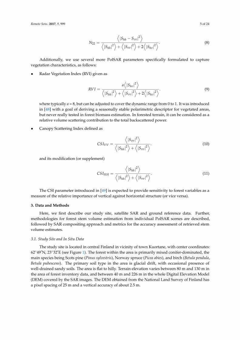
The study site is located in central Finland in vicinity of town Kuortane, with center coordinates:62◦49′N, 23◦32′E (see Figure 1). The forest within the area is primarily mixed conifer-dominated, themain species being Scots pine (Pinus sylvestris), Norway spruce (Picea abies), and birch (Betula pendula,Betula pubescens). The primary soil type in the area is glacial drift, with occasional presence ofwell-drained sandy soils. The area is flat to hilly. Terrain elevation varies between 80 m and 130 m inthe area of forest inventory data, and between 40 m and 226 m in the whole Digital Elevation Model(DEM) covered by the SAR images. The DEM obtained from the National Land Survey of Finland hasa pixel spacing of 25 m and a vertical accuracy of about 2.5 m.

Remote Sens. 2017, 9, 999 6 of 24

Remote Sens. 2017, 9, 999 6 of 24

Figure 1. Study site location.

3.2. SAR Data

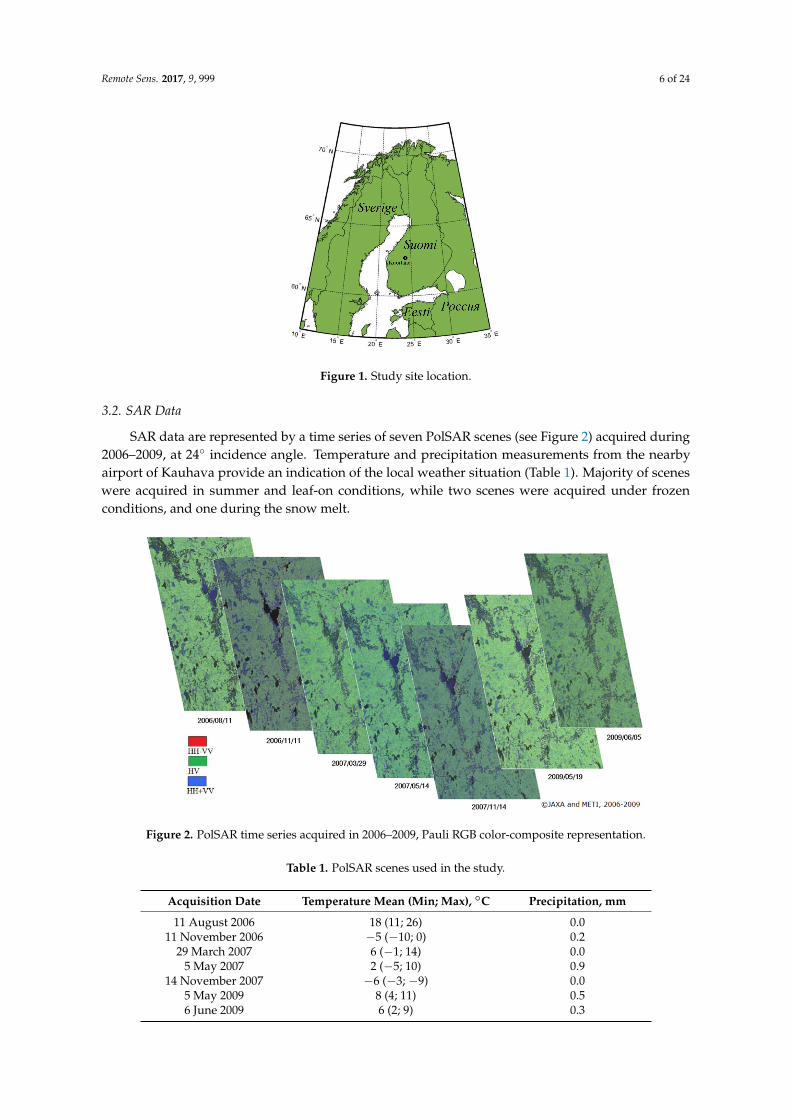
SAR data are represented by a time series of seven PolSAR scenes (see Figure 2) acquired during 2006–2009, at 24° incidence angle. Temperature and precipitation measurements from the nearby airport of Kauhava provide an indication of the local weather situation (Table 1). Majority of scenes were acquired in summer and leaf-on conditions, while two scenes were acquired under frozen conditions, and one during the snow melt.

Figure 2. PolSAR time series acquired in 2006–2009, Pauli RGB color-composite representation.

Table 1. PolSAR scenes used in the study.

Acquisition Date Temperature Mean (Min; Max), °C Precipitation, mm 11 August 2006 18 (11; 26) 0.0

11 November 2006 −5 (−10; 0) 0.2 29 March 2007 6 (−1; 14) 0.0

5 May 2007 2 (−5; 10) 0.9 14 November 2007 −6 (−3; −9) 0.0

5 May 2009 8 (4; 11) 0.5 6 June 2009 6 (2; 9) 0.3

Figure 1. Study site location.

3.2. SAR Data

SAR data are represented by a time series of seven PolSAR scenes (see Figure 2) acquired during2006–2009, at 24◦ incidence angle. Temperature and precipitation measurements from the nearbyairport of Kauhava provide an indication of the local weather situation (Table 1). Majority of sceneswere acquired in summer and leaf-on conditions, while two scenes were acquired under frozenconditions, and one during the snow melt.

Remote Sens. 2017, 9, 999 6 of 24

Figure 1. Study site location.

3.2. SAR Data

SAR data are represented by a time series of seven PolSAR scenes (see Figure 2) acquired during 2006–2009, at 24° incidence angle. Temperature and precipitation measurements from the nearby airport of Kauhava provide an indication of the local weather situation (Table 1). Majority of scenes were acquired in summer and leaf-on conditions, while two scenes were acquired under frozen conditions, and one during the snow melt.

Figure 2. PolSAR time series acquired in 2006–2009, Pauli RGB color-composite representation.

Table 1. PolSAR scenes used in the study.

Acquisition Date Temperature Mean (Min; Max), °C Precipitation, mm 11 August 2006 18 (11; 26) 0.0

11 November 2006 −5 (−10; 0) 0.2 29 March 2007 6 (−1; 14) 0.0

5 May 2007 2 (−5; 10) 0.9 14 November 2007 −6 (−3; −9) 0.0

5 May 2009 8 (4; 11) 0.5 6 June 2009 6 (2; 9) 0.3

Figure 2. PolSAR time series acquired in 2006–2009, Pauli RGB color-composite representation.

Table 1. PolSAR scenes used in the study.

Acquisition Date Temperature Mean (Min; Max), ◦C Precipitation, mm

11 August 2006 18 (11; 26) 0.011 November 2006 −5 (−10; 0) 0.2

29 March 2007 6 (−1; 14) 0.05 May 2007 2 (−5; 10) 0.9

14 November 2007 −6 (−3; −9) 0.05 May 2009 8 (4; 11) 0.56 June 2009 6 (2; 9) 0.3

Remote Sens. 2017, 9, 999 7 of 24

3.3. Reference Data

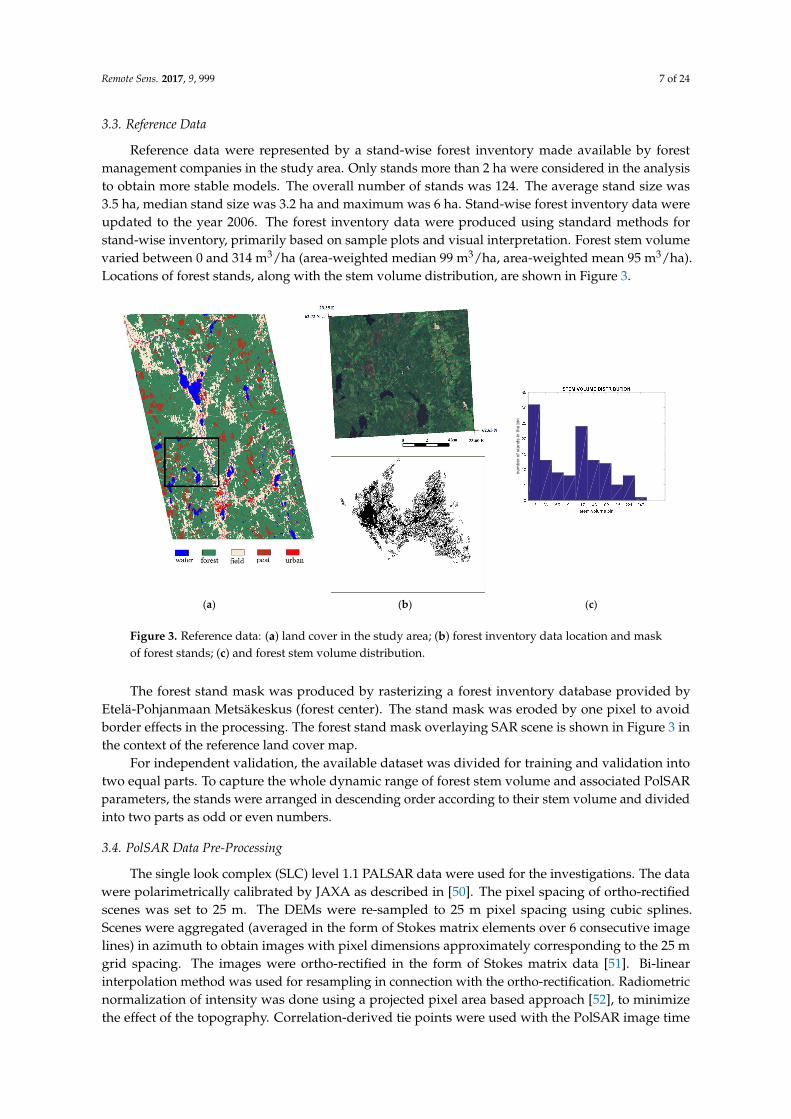
Reference data were represented by a stand-wise forest inventory made available by forestmanagement companies in the study area. Only stands more than 2 ha were considered in the analysisto obtain more stable models. The overall number of stands was 124. The average stand size was3.5 ha, median stand size was 3.2 ha and maximum was 6 ha. Stand-wise forest inventory data wereupdated to the year 2006. The forest inventory data were produced using standard methods forstand-wise inventory, primarily based on sample plots and visual interpretation. Forest stem volumevaried between 0 and 314 m3/ha (area-weighted median 99 m3/ha, area-weighted mean 95 m3/ha).Locations of forest stands, along with the stem volume distribution, are shown in Figure 3.

Remote Sens. 2017, 9, 999 7 of 24

3.3. Reference Data

Reference data were represented by a stand-wise forest inventory made available by forest management companies in the study area. Only stands more than 2 ha were considered in the analysis to obtain more stable models. The overall number of stands was 124. The average stand size was 3.5 ha, median stand size was 3.2 ha and maximum was 6 ha. Stand-wise forest inventory data were updated to the year 2006. The forest inventory data were produced using standard methods for stand-wise inventory, primarily based on sample plots and visual interpretation. Forest stem volume varied between 0 and 314 m3/ha (area-weighted median 99 m3/ha, area-weighted mean 95 m3/ha). Locations of forest stands, along with the stem volume distribution, are shown in Figure 3.

(a) (b) (c)

Figure 3. Reference data: (a) land cover in the study area; (b) forest inventory data location and mask of forest stands; (c) and forest stem volume distribution.

The forest stand mask was produced by rasterizing a forest inventory database provided by Etelä-Pohjanmaan Metsäkeskus (forest center). The stand mask was eroded by one pixel to avoid border effects in the processing. The forest stand mask overlaying SAR scene is shown in Figure 3 in the context of the reference land cover map.

For independent validation, the available dataset was divided for training and validation into two equal parts. To capture the whole dynamic range of forest stem volume and associated PolSAR parameters, the stands were arranged in descending order according to their stem volume and divided into two parts as odd or even numbers.

3.4. PolSAR Data Pre-Processing

The single look complex (SLC) level 1.1 PALSAR data were used for the investigations. The data were polarimetrically calibrated by JAXA as described in [50]. The pixel spacing of ortho-rectified scenes was set to 25 m. The DEMs were re-sampled to 25 m pixel spacing using cubic splines. Scenes were aggregated (averaged in the form of Stokes matrix elements over 6 consecutive image lines) in azimuth to obtain images with pixel dimensions approximately corresponding to the 25 m grid spacing. The images were ortho-rectified in the form of Stokes matrix data [51]. Bi-linear interpolation method was used for resampling in connection with the ortho-rectification. Radiometric normalization of intensity was done using a projected pixel area based approach [52], to minimize the effect of the topography. Correlation-derived tie points were used with the PolSAR image time series as the geo-location information was not precise enough. Map-derived ground control points

num

ber o

f sta

nds

in th

e bi

n

Figure 3. Reference data: (a) land cover in the study area; (b) forest inventory data location and maskof forest stands; (c) and forest stem volume distribution.

The forest stand mask was produced by rasterizing a forest inventory database provided byEtelä-Pohjanmaan Metsäkeskus (forest center). The stand mask was eroded by one pixel to avoidborder effects in the processing. The forest stand mask overlaying SAR scene is shown in Figure 3 inthe context of the reference land cover map.

For independent validation, the available dataset was divided for training and validation intotwo equal parts. To capture the whole dynamic range of forest stem volume and associated PolSARparameters, the stands were arranged in descending order according to their stem volume and dividedinto two parts as odd or even numbers.

3.4. PolSAR Data Pre-Processing

The single look complex (SLC) level 1.1 PALSAR data were used for the investigations. The datawere polarimetrically calibrated by JAXA as described in [50]. The pixel spacing of ortho-rectifiedscenes was set to 25 m. The DEMs were re-sampled to 25 m pixel spacing using cubic splines.Scenes were aggregated (averaged in the form of Stokes matrix elements over 6 consecutive imagelines) in azimuth to obtain images with pixel dimensions approximately corresponding to the 25 mgrid spacing. The images were ortho-rectified in the form of Stokes matrix data [51]. Bi-linearinterpolation method was used for resampling in connection with the ortho-rectification. Radiometricnormalization of intensity was done using a projected pixel area based approach [52], to minimizethe effect of the topography. Correlation-derived tie points were used with the PolSAR image time

Remote Sens. 2017, 9, 999 8 of 24

series as the geo-location information was not precise enough. Map-derived ground control pointswere used to revise the geo-location computed from the state vector and time code data in the ALOSPALSAR products.

Afterwards, the covariance/coherency matrix was formed, followed by speckle filtering (medianfiltering of 3 × 3). The estimate of the Faraday rotation angle [53,54] was within the 2◦ range indicatingno expected influence on biophysical parameter retrieval [55].

To compensate for the slope effect, the polarization orientation angles (POAs) were derived fromthe circular polarization algorithm [56], as shown below:

θ =14

[arctan

(2Re{T23}T22 − T33

)], (12)

where θ is the phase difference between the right-right and left-left circular polarizations, and Tpq is acorresponding element of polarimetric coherence matrix. After the POA estimation, a new coherencematrix is formed using unitary line of sight rotation matrix:

[T3_θ] = [I_θ] ∗ [T3] ∗ [I_θ]−1, (13)

With line of sight (LOS) matrix

[I_θ] =

1 0 00 cos 2θ sin 2θ

0 − sin 2θ cos 2θ

. (14)

All analysis was performed using stand-wise averaged SAR data. The averaged stand-wise valuesof elements of polarimetric covariance/coherence matrix were calculated in the power domain byaveraging all pixel intensity values within each eroded stand (one-pixel erosion was applied).

3.5. SAR Based Estimation of Stem Volume

Forest stem volume was estimated based on two PolSAR parameters: cross-pol backscatter andco-pol coherence. Both parameters exhibit nonlinear dependence on biomass, with many suitablemodels available for their inversion [38,39,57].

In this study, due to presence of considerable reference data and to avoid peculiarities of, e.g.,solving a system of two nonlinear equations, we used a non-parametric estimation technique: k nearestneighbor (kNN) regression method. Different nearest neighbor regression approaches became populartools in estimating forest parameters from remotely sensed data [58–62]. Particularly, a multisourcenational forest inventory (NFI) in Finland is based on k nearest neighbor (kNN) approach [60,61].Within the kNN regression methodology, the distance functions (between neighbors), number (k) ofnearest neighbors and methods of their search, as well as weighting of the chosen neighbors, vary.

Here, we suggest estimating the forest stem volume of each stand as an average of forest standvalues of the k nearest forest stands in the feature space of chosen PolSAR parameters. Here, we firstdescribe measures and procedures needed for the kNN regression approach, and then proceed to thealgorithm description.

Parameter k, the number of nearest neighbors, is an external parameter of the method. Distancebetween stands is calculated in the feature space of PolSAR parameters. Here, we chose p = 2meaningful PolSAR parameters: HV backscatter and HHVV coherence. As their dynamic range varies,a linear stretching (standardization) was performed to have both coherence and backscatter withinthe [0; 1] dynamic range. In principle, such procedure is applicable also to other PolSAR parametersshould they be chosen for predicting stem volume, such as e.g., RVI or various PolSAR ratios.

Distance d from evaluated stand x to reference stand y (in the feature space of dimensionality p),is, in general case, a Minkowski distance:

Remote Sens. 2017, 9, 999 9 of 24

d =(∑ p

i=1(|xi − yi|)q)1/q

. (15)

Here, we used q = 2, that is simply the Euclidean distance.Finally, an estimate of the forest stem volume Vest

x was obtained as

Vestx = (1/k)∑ k

y=1Vy, (16)

where x and y are forest stand indices, Vy is the stem volume of y-th nearest forest stand, and k is thenumber of nearest stands and the parameter of the kNN algorithm.

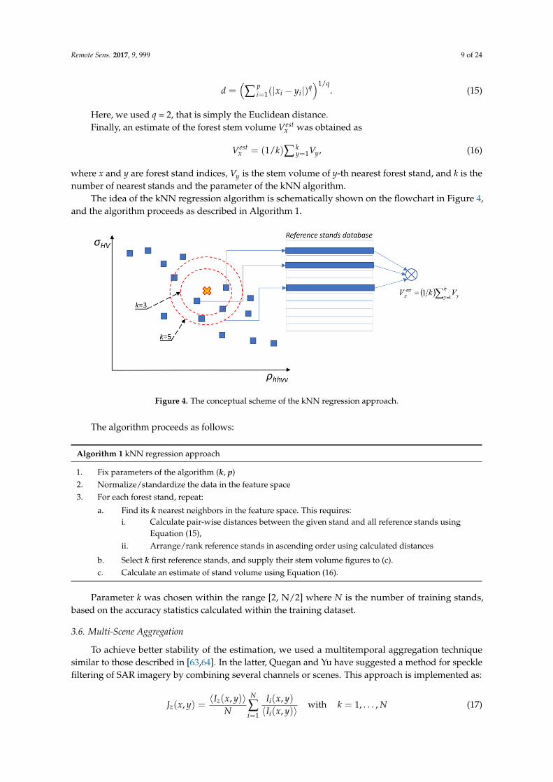
The idea of the kNN regression algorithm is schematically shown on the flowchart in Figure 4,and the algorithm proceeds as described in Algorithm 1.

Remote Sens. 2017, 9, 999 9 of 24

( )( ) qp

i

q

ii yxd/1

1 =−= . (15)

Here, we used q = 2, that is simply the Euclidean distance. Finally, an estimate of the forest stem volume est

xV was obtained as

( ) == k

y yestx VkV

11 , (16)

where x and y are forest stand indices, yV is the stem volume of y-th nearest forest stand, and k is

the number of nearest stands and the parameter of the kNN algorithm. The idea of the kNN regression algorithm is schematically shown on the flowchart in Figure 4,

and the algorithm proceeds as described in Algorithm 1.

Figure 4. The conceptual scheme of the kNN regression approach.

The algorithm proceeds as follows:

Algorithm 1 kNN regression approach1. Fix parameters of the algorithm (k, p) 2. Normalize/standardize the data in the feature space 3. For each forest stand, repeat:

a. Find its k nearest neighbors in the feature space. This requires: i. Calculate pair-wise distances between the given stand and all

reference stands using Equation (15), ii. Arrange/rank reference stands in ascending order using calculated

distances b. Select k first reference stands, and supply their stem volume figures to (c). c. Calculate an estimate of stand volume using Equation (16).

Parameter k was chosen within the range [2, N/2] where N is the number of training stands, based on the accuracy statistics calculated within the training dataset.

3.6. Multi-Scene Aggregation

To achieve better stability of the estimation, we used a multitemporal aggregation technique similar to those described in [63,64]. In the latter, Quegan and Yu have suggested a method for speckle filtering of SAR imagery by combining several channels or scenes. This approach is implemented as:

=

==N

i i

izz Nk

yxI

yxI

N

yxIyxJ

1,...,1with

),(),(),(

),( (17)

Figure 4. The conceptual scheme of the kNN regression approach.

The algorithm proceeds as follows:

Algorithm 1 kNN regression approach

1. Fix parameters of the algorithm (k, p)2. Normalize/standardize the data in the feature space3. For each forest stand, repeat:

a. Find its k nearest neighbors in the feature space. This requires:i. Calculate pair-wise distances between the given stand and all reference stands using

Equation (15),ii. Arrange/rank reference stands in ascending order using calculated distances

b. Select k first reference stands, and supply their stem volume figures to (c).c. Calculate an estimate of stand volume using Equation (16).

Parameter k was chosen within the range [2, N/2] where N is the number of training stands,based on the accuracy statistics calculated within the training dataset.

3.6. Multi-Scene Aggregation

To achieve better stability of the estimation, we used a multitemporal aggregation techniquesimilar to those described in [63,64]. In the latter, Quegan and Yu have suggested a method for specklefiltering of SAR imagery by combining several channels or scenes. This approach is implemented as:

Jz(x, y) =〈Iz(x, y)〉

N

N

∑i=1

Ii(x, y)〈Ii(x, y)〉 with k = 1, . . . , N (17)

Remote Sens. 2017, 9, 999 10 of 24

where, at pixel position (x,y), Jz(x, y) is the intensity of composite image (coherence matrix element),Ii(x, y) is the intensity of i-th input image, <Ii(x, y)> is the local average intensity of i-th input image,and N is the number of combined images.

Similar methodology is used here to combine PolSAR scenes in the intensity domain, beforecalculating PolSAR parameters of interest and performing stem-volume estimation. For each pixellocation (x, y), each element of the coherence matrix is combined using Equation (17). We expect thisapproach to work best with images acquired in similar environmental conditions (where there is nobias caused by change of scattering mechanism due to, e.g., frozen state of forest or flooded terrain).Particular combinations of PolSAR scenes tested in the study, along with the results of the biomassestimation, are reported in Section 4.2.

3.7. Accuracy Analysis

Performance of the estimation approach was quantitatively evaluated using Root Mean SquareError (RMSE) as

RMSE =

√1N ∑ N

i=1

(Vmeas

i −Vesti)2, (18)

where N is the number of forest stands, and Vmeasi and Vest

i are measured and estimated values offorest stem volume for i-th stand, respectively. Further, relative RMSE was calculated by dividingabsolute RMSE values by mean stem volume within the study site.

RMSE% = (RMSE ∗ N)/(∑ N

i=1(Vmeasi )

). (19)

In addition, the Pearson correlation coefficient r and coefficient of determination R2 were used forinterpretation, as traditionally adopted for this purpose in the remote sensing literature.

4. Results

Here, we first describe and discuss inter-dependencies between stand-wise estimates of differentPolSAR parameters, as well as their relation to forest stem volume. Then, we chose two representativePolSAR parameters to predict the forest stem volume, namely co-polarization coherence andcross-polarization backscatter. Later, forest stem volume is estimated using the kNN method based ondifferent combinations of these PolSAR parameters, as well as their multitemporal composites.

4.1. Temporal Dependence of PolSAR Parameters and Relation to Stem Volume

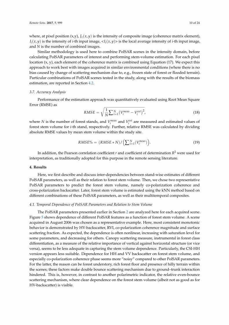
The PolSAR parameters presented earlier in Section 2 are analyzed here for each acquired scene.Figure 5 shows dependence of different PolSAR features as a function of forest stem volume. A sceneacquired in August 2006 was chosen as a representative example. Here, most consistent monotonicbehavior is demonstrated by HV-backscatter, RVI, co-polarization coherence magnitude and surfacescattering fraction. As expected, the dependence is often nonlinear, increasing with saturation level forsome parameters, and decreasing for others. Canopy scattering measure, instrumental in forest classdifferentiation, as a measure of the relative importance of vertical against horizontal structure (or viceversa), seems to be less adequate in capturing the stem volume dependence. Particularly, the CSI-HHversion appears less suitable. Dependence for HH and VV backscatter on forest stem volume, andespecially co-polarization coherence phase seems more “noisy” compared to other PolSAR parameters.For the latter, the reason can be forest understory, rich forest floor and presence of hilly terrain withinthe scenes; these factors make double bounce scattering mechanism due to ground–trunk interactionhindered. This is, however, in contrast to another polarimetric indicator, the relative even-bouncescattering mechanism, where clear dependence on the forest stem volume (albeit not as good as forHV-backscatter) is visible.

Remote Sens. 2017, 9, 999 11 of 24

Remote Sens. 2017, 9, 999 11 of 24

further biomass retrieval), as the dependence can be nonlinear. In fact, Figure 5 clearly demonstrates that the assumption [11,26] on linear dependence between the forest stem volume and the majority of PolSAR parameters often fails; such approximation seems possible only over a certain range of the forest biomass values.

Figure 5. Dependence of PolSAR features on forest stem volume for selected scene (August 2006). Figure 5. Dependence of PolSAR features on forest stem volume for selected scene (August 2006).

It is important to keep in mind that low correlation between forest stem volume and a specificPolSAR parameter does not necessarily suggest that the given parameter is suboptimal (e.g., for further

Remote Sens. 2017, 9, 999 12 of 24

biomass retrieval), as the dependence can be nonlinear. In fact, Figure 5 clearly demonstrates thatthe assumption [11,26] on linear dependence between the forest stem volume and the majority ofPolSAR parameters often fails; such approximation seems possible only over a certain range of theforest biomass values.

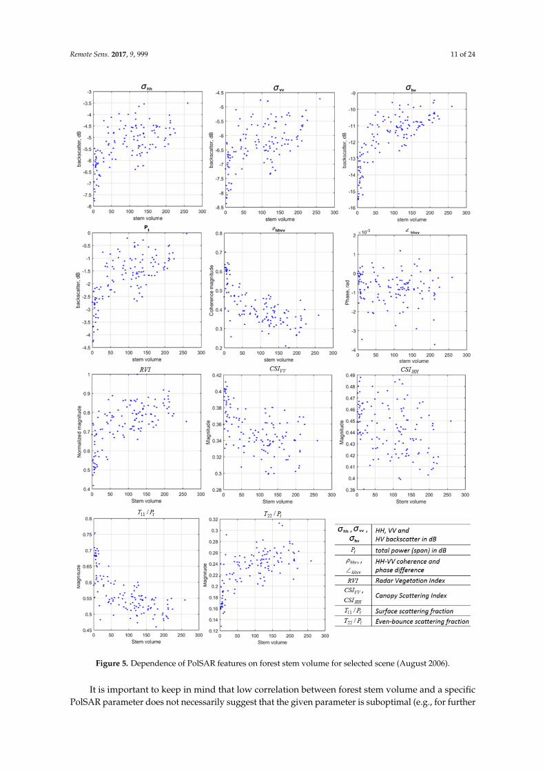
On the other hand, it is important to investigate the temporal dependence (or stability) of PolSARparameters in relation to stem volume, as well as levels of correlation between different PolSARparameters. The latter can help to seed out unnecessary (or unstable) parameters, while the formercan suggest optimal conditions for the image acquisition, and hint on possible ways to aggregatedifferent PolSAR scenes. As the Kuortane vicinities belong to intensively managed forest areas, it waseasy to detect effects associated with clearcutting, particularly on the stand level. Several stands weredetected as clear-cut especially within the last two-three scenes compared to other images, with themajority of PolSAR parameters being suitable to detect these changes. An example with cross-polbackscatter is shown in Figure 6. It is important to note that only non-cut stands (during the time spanof 2006–2009) were used in calculating multitemporal statistics shown further, as well as in the foreststem volume retrieval.

Remote Sens. 2017, 9, 999 12 of 24

stem volume m3/ha stem volume m3/ha

stem volume m3/ha

On the other hand, it is important to investigate the temporal dependence (or stability) of PolSAR parameters in relation to stem volume, as well as levels of correlation between different PolSAR parameters. The latter can help to seed out unnecessary (or unstable) parameters, while the former can suggest optimal conditions for the image acquisition, and hint on possible ways to aggregate different PolSAR scenes. As the Kuortane vicinities belong to intensively managed forest areas, it was easy to detect effects associated with clearcutting, particularly on the stand level. Several stands were detected as clear-cut especially within the last two-three scenes compared to other images, with the majority of PolSAR parameters being suitable to detect these changes. An example with cross-pol backscatter is shown in Figure 6. It is important to note that only non-cut stands (during the time span of 2006–2009) were used in calculating multitemporal statistics shown further, as well as in the forest stem volume retrieval.

(a) (b)

(c)

Figure 6. Temporal dynamics of cross-polarization backscatter reveals changes on stand level, with removal of at least six stands detected: (a) 11 August 2006; (b) 14 May 2007; and (c) 5 June 2009.

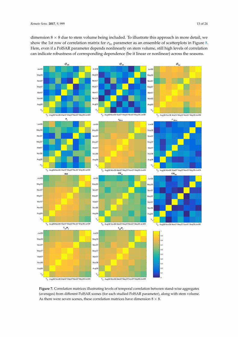
Figure 7 shows cross-correlation matrices for different PolSAR parameter in question, to assess the temporal stability between scenes. Another typical approach is to visualize these correlations explicitly as scatter-plots (e.g., as in [38]). In this situation, a level of 1 corresponds to fully linearly correlated dependence between corresponding two scenes (modulus of Pearson’s correlation coefficient). Each pixel in respective correlation matrices corresponds to one scatterplot. As altogether there were seven ALOS PALSAR scenes, the correlation matrices for each PolSAR parameter have dimension 8 × 8 due to stem volume being included. To illustrate this approach in more detail, we

show the 1st row of correlation matrix for hvσ parameter as an ensemble of scatterplots in Figure 8. Here, even if a PolSAR parameter depends nonlinearly on stem volume, still high levels of correlation can indicate robustness of corresponding dependence (be it linear or nonlinear) across the seasons.

Figure 6. Temporal dynamics of cross-polarization backscatter reveals changes on stand level, withremoval of at least six stands detected: (a) 11 August 2006; (b) 14 May 2007; and (c) 5 June 2009.

Figure 7 shows cross-correlation matrices for different PolSAR parameter in question, to assessthe temporal stability between scenes. Another typical approach is to visualize these correlationsexplicitly as scatter-plots (e.g., as in [38]). In this situation, a level of 1 corresponds to fullylinearly correlated dependence between corresponding two scenes (modulus of Pearson’s correlationcoefficient). Each pixel in respective correlation matrices corresponds to one scatterplot. As altogetherthere were seven ALOS PALSAR scenes, the correlation matrices for each PolSAR parameter have

Remote Sens. 2017, 9, 999 13 of 24

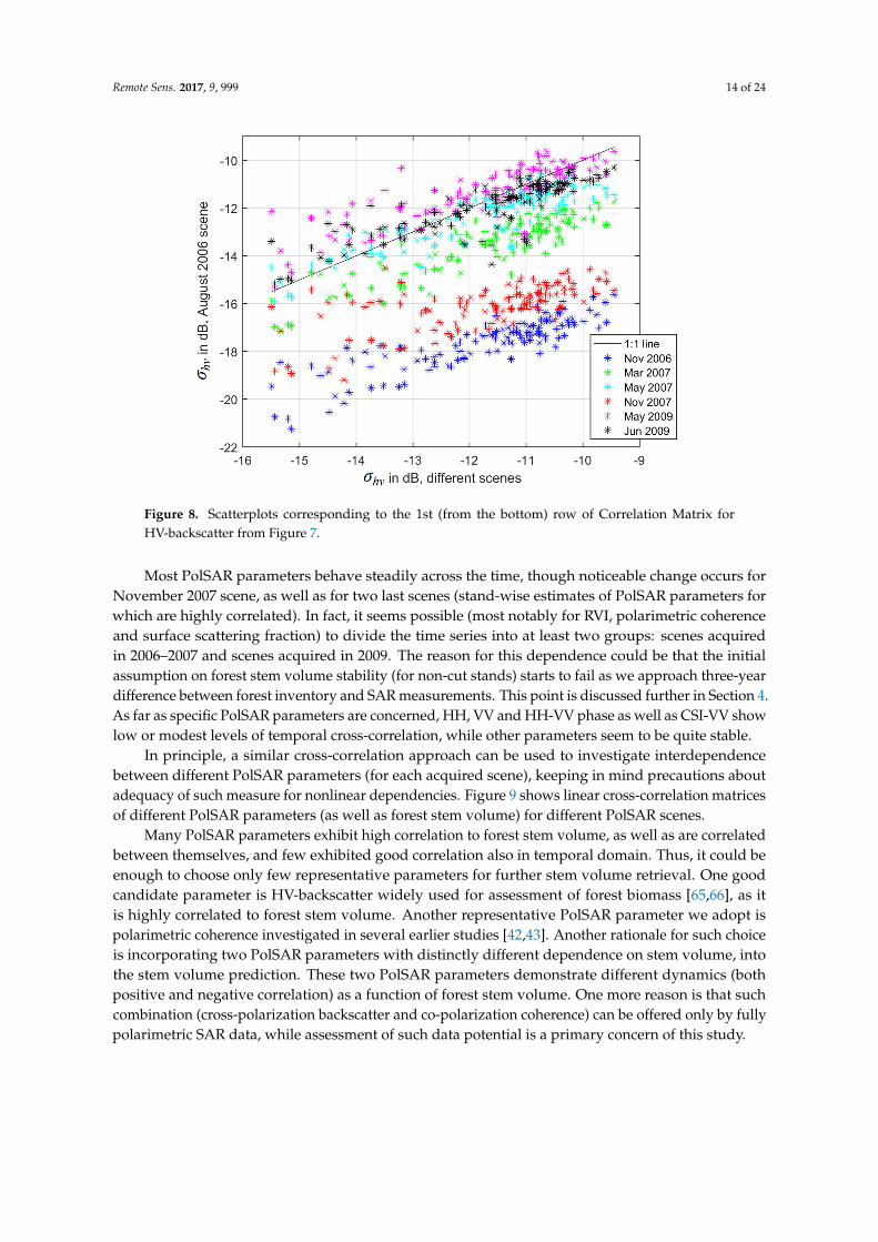
dimension 8 × 8 due to stem volume being included. To illustrate this approach in more detail, weshow the 1st row of correlation matrix for σhv parameter as an ensemble of scatterplots in Figure 8.Here, even if a PolSAR parameter depends nonlinearly on stem volume, still high levels of correlationcan indicate robustness of corresponding dependence (be it linear or nonlinear) across the seasons.Remote Sens. 2017, 9, 999 13 of 24

Figure 7. Correlation matrices illustrating levels of temporal correlation between stand-wise aggregates (averages) from different PolSAR scenes (for each studied PolSAR parameter), along with stem volume. As there were seven scenes, these correlation matrices have dimension 8 × 8.

Figure 7. Correlation matrices illustrating levels of temporal correlation between stand-wise aggregates(averages) from different PolSAR scenes (for each studied PolSAR parameter), along with stem volume.As there were seven scenes, these correlation matrices have dimension 8 × 8.

Remote Sens. 2017, 9, 999 14 of 24Remote Sens. 2017, 9, 999 14 of 24

Figure 8. Scatterplots corresponding to the 1st (from the bottom) row of Correlation Matrix for HV-backscatter from Figure 7.

Most PolSAR parameters behave steadily across the time, though noticeable change occurs for November 2007 scene, as well as for two last scenes (stand-wise estimates of PolSAR parameters for which are highly correlated). In fact, it seems possible (most notably for RVI, polarimetric coherence and surface scattering fraction) to divide the time series into at least two groups: scenes acquired in 2006–2007 and scenes acquired in 2009. The reason for this dependence could be that the initial assumption on forest stem volume stability (for non-cut stands) starts to fail as we approach three-year difference between forest inventory and SAR measurements. This point is discussed further in Section 4. As far as specific PolSAR parameters are concerned, HH, VV and HH-VV phase as well as CSI-VV show low or modest levels of temporal cross-correlation, while other parameters seem to be quite stable.

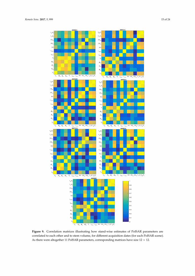
In principle, a similar cross-correlation approach can be used to investigate interdependence between different PolSAR parameters (for each acquired scene), keeping in mind precautions about adequacy of such measure for nonlinear dependencies. Figure 9 shows linear cross-correlation matrices of different PolSAR parameters (as well as forest stem volume) for different PolSAR scenes.

Many PolSAR parameters exhibit high correlation to forest stem volume, as well as are correlated between themselves, and few exhibited good correlation also in temporal domain. Thus, it could be enough to choose only few representative parameters for further stem volume retrieval. One good candidate parameter is HV-backscatter widely used for assessment of forest biomass [65,66], as it is highly correlated to forest stem volume. Another representative PolSAR parameter we adopt is polarimetric coherence investigated in several earlier studies [42,43]. Another rationale for such choice is incorporating two PolSAR parameters with distinctly different dependence on stem volume, into the stem volume prediction. These two PolSAR parameters demonstrate different dynamics (both positive and negative correlation) as a function of forest stem volume. One more reason is that such combination (cross-polarization backscatter and co-polarization coherence) can be offered only by fully polarimetric SAR data, while assessment of such data potential is a primary concern of this study.

Figure 8. Scatterplots corresponding to the 1st (from the bottom) row of Correlation Matrix forHV-backscatter from Figure 7.

Most PolSAR parameters behave steadily across the time, though noticeable change occurs forNovember 2007 scene, as well as for two last scenes (stand-wise estimates of PolSAR parameters forwhich are highly correlated). In fact, it seems possible (most notably for RVI, polarimetric coherenceand surface scattering fraction) to divide the time series into at least two groups: scenes acquiredin 2006–2007 and scenes acquired in 2009. The reason for this dependence could be that the initialassumption on forest stem volume stability (for non-cut stands) starts to fail as we approach three-yeardifference between forest inventory and SAR measurements. This point is discussed further in Section 4.As far as specific PolSAR parameters are concerned, HH, VV and HH-VV phase as well as CSI-VV showlow or modest levels of temporal cross-correlation, while other parameters seem to be quite stable.

In principle, a similar cross-correlation approach can be used to investigate interdependencebetween different PolSAR parameters (for each acquired scene), keeping in mind precautions aboutadequacy of such measure for nonlinear dependencies. Figure 9 shows linear cross-correlation matricesof different PolSAR parameters (as well as forest stem volume) for different PolSAR scenes.

Many PolSAR parameters exhibit high correlation to forest stem volume, as well as are correlatedbetween themselves, and few exhibited good correlation also in temporal domain. Thus, it could beenough to choose only few representative parameters for further stem volume retrieval. One goodcandidate parameter is HV-backscatter widely used for assessment of forest biomass [65,66], as itis highly correlated to forest stem volume. Another representative PolSAR parameter we adopt ispolarimetric coherence investigated in several earlier studies [42,43]. Another rationale for such choiceis incorporating two PolSAR parameters with distinctly different dependence on stem volume, intothe stem volume prediction. These two PolSAR parameters demonstrate different dynamics (bothpositive and negative correlation) as a function of forest stem volume. One more reason is that suchcombination (cross-polarization backscatter and co-polarization coherence) can be offered only by fullypolarimetric SAR data, while assessment of such data potential is a primary concern of this study.

Remote Sens. 2017, 9, 999 15 of 24

Remote Sens. 2017, 9, 999 15 of 24

Figure 9. Correlation matrices illustrating how stand-wise estimates of PolSAR parameters are correlated to each other and to stem volume, for different acquisition dates (for each PolSAR scene). As there were altogether 11 PolSAR parameters, corresponding matrices have size 12 × 12.

Figure 9. Correlation matrices illustrating how stand-wise estimates of PolSAR parameters arecorrelated to each other and to stem volume, for different acquisition dates (for each PolSAR scene).As there were altogether 11 PolSAR parameters, corresponding matrices have size 12 × 12.

Remote Sens. 2017, 9, 999 16 of 24

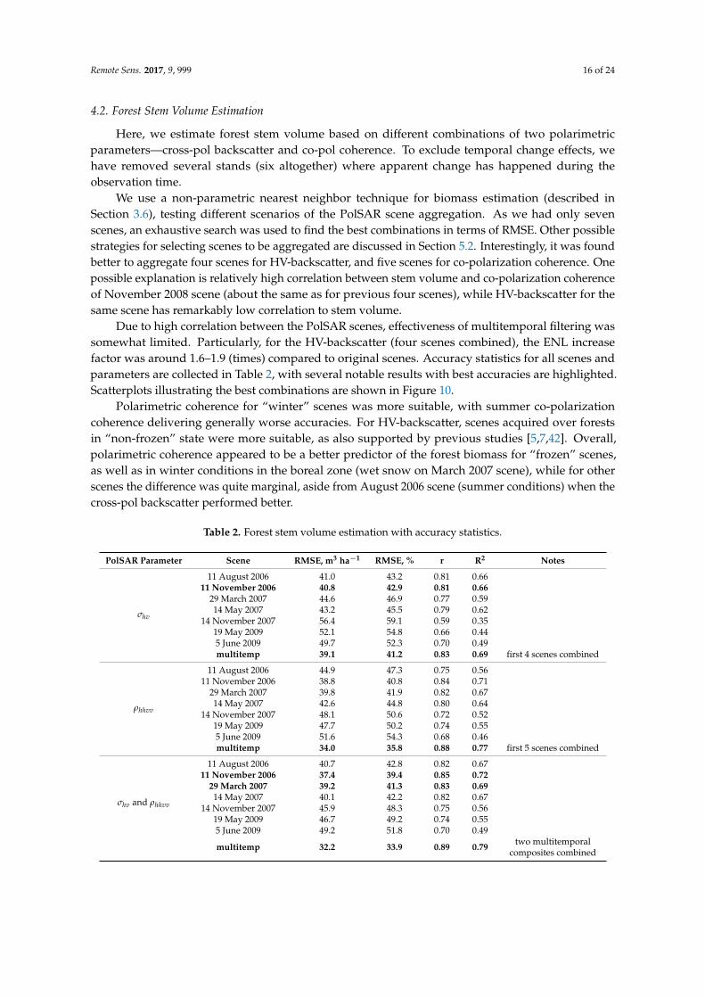
4.2. Forest Stem Volume Estimation

Here, we estimate forest stem volume based on different combinations of two polarimetricparameters—cross-pol backscatter and co-pol coherence. To exclude temporal change effects, wehave removed several stands (six altogether) where apparent change has happened during theobservation time.

We use a non-parametric nearest neighbor technique for biomass estimation (described inSection 3.6), testing different scenarios of the PolSAR scene aggregation. As we had only sevenscenes, an exhaustive search was used to find the best combinations in terms of RMSE. Other possiblestrategies for selecting scenes to be aggregated are discussed in Section 5.2. Interestingly, it was foundbetter to aggregate four scenes for HV-backscatter, and five scenes for co-polarization coherence. Onepossible explanation is relatively high correlation between stem volume and co-polarization coherenceof November 2008 scene (about the same as for previous four scenes), while HV-backscatter for thesame scene has remarkably low correlation to stem volume.

Due to high correlation between the PolSAR scenes, effectiveness of multitemporal filtering wassomewhat limited. Particularly, for the HV-backscatter (four scenes combined), the ENL increasefactor was around 1.6–1.9 (times) compared to original scenes. Accuracy statistics for all scenes andparameters are collected in Table 2, with several notable results with best accuracies are highlighted.Scatterplots illustrating the best combinations are shown in Figure 10.

Polarimetric coherence for “winter” scenes was more suitable, with summer co-polarizationcoherence delivering generally worse accuracies. For HV-backscatter, scenes acquired over forestsin “non-frozen” state were more suitable, as also supported by previous studies [5,7,42]. Overall,polarimetric coherence appeared to be a better predictor of the forest biomass for “frozen” scenes,as well as in winter conditions in the boreal zone (wet snow on March 2007 scene), while for otherscenes the difference was quite marginal, aside from August 2006 scene (summer conditions) when thecross-pol backscatter performed better.

Table 2. Forest stem volume estimation with accuracy statistics.

PolSAR Parameter Scene RMSE, m3 ha−1 RMSE, % r R2 Notes

σhv

11 August 2006 41.0 43.2 0.81 0.6611 November 2006 40.8 42.9 0.81 0.66

29 March 2007 44.6 46.9 0.77 0.5914 May 2007 43.2 45.5 0.79 0.62

14 November 2007 56.4 59.1 0.59 0.3519 May 2009 52.1 54.8 0.66 0.445 June 2009 49.7 52.3 0.70 0.49multitemp 39.1 41.2 0.83 0.69 first 4 scenes combined

ρhhvv

11 August 2006 44.9 47.3 0.75 0.5611 November 2006 38.8 40.8 0.84 0.71

29 March 2007 39.8 41.9 0.82 0.6714 May 2007 42.6 44.8 0.80 0.64

14 November 2007 48.1 50.6 0.72 0.5219 May 2009 47.7 50.2 0.74 0.555 June 2009 51.6 54.3 0.68 0.46multitemp 34.0 35.8 0.88 0.77 first 5 scenes combined

σhv and ρhhvv

11 August 2006 40.7 42.8 0.82 0.6711 November 2006 37.4 39.4 0.85 0.72

29 March 2007 39.2 41.3 0.83 0.6914 May 2007 40.1 42.2 0.82 0.67

14 November 2007 45.9 48.3 0.75 0.5619 May 2009 46.7 49.2 0.74 0.555 June 2009 49.2 51.8 0.70 0.49

multitemp 32.2 33.9 0.89 0.79 two multitemporalcomposites combined

Remote Sens. 2017, 9, 999 17 of 24

Remote Sens. 2017, 9, 999 17 of 24

(a) (b) (c)

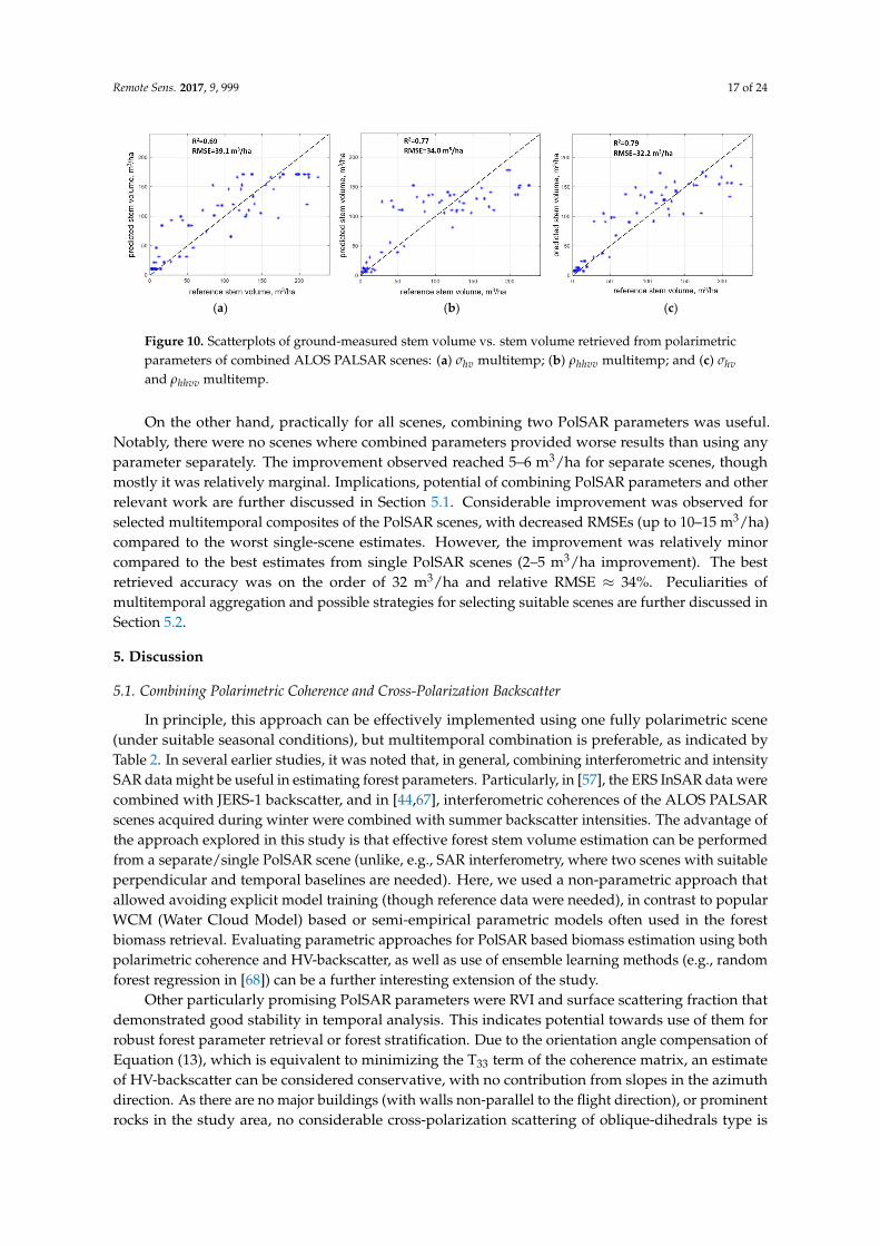
Figure 10. Scatterplots of ground-measured stem volume vs. stem volume retrieved from polarimetric parameters of combined ALOS PALSAR scenes: (a)

hvσ multitemp; (b) hhvvρ multitemp; and (c)

hvσ and hhvvρ multitemp.

On the other hand, practically for all scenes, combining two PolSAR parameters was useful. Notably, there were no scenes where combined parameters provided worse results than using any parameter separately. The improvement observed reached 5–6 m3/ha for separate scenes, though mostly it was relatively marginal. Implications, potential of combining PolSAR parameters and other relevant work are further discussed in Section 5.1. Considerable improvement was observed for selected multitemporal composites of the PolSAR scenes, with decreased RMSEs (up to 10–15 m3/ha) compared to the worst single-scene estimates. However, the improvement was relatively minor compared to the best estimates from single PolSAR scenes (2–5 m3/ha improvement). The best retrieved accuracy was on the order of 32 m3/ha and relative RMSE ≈ 34%. Peculiarities of multitemporal aggregation and possible strategies for selecting suitable scenes are further discussed in Section 5.2.

5. Discussion

5.1. Combining Polarimetric Coherence and Cross-Polarization Backscatter

In principle, this approach can be effectively implemented using one fully polarimetric scene (under suitable seasonal conditions), but multitemporal combination is preferable, as indicated by Table 2. In several earlier studies, it was noted that, in general, combining interferometric and intensity SAR data might be useful in estimating forest parameters. Particularly, in [57], the ERS InSAR data were combined with JERS-1 backscatter, and in [44,67], interferometric coherences of the ALOS PALSAR scenes acquired during winter were combined with summer backscatter intensities. The advantage of the approach explored in this study is that effective forest stem volume estimation can be performed from a separate/single PolSAR scene (unlike, e.g., SAR interferometry, where two scenes with suitable perpendicular and temporal baselines are needed). Here, we used a non-parametric approach that allowed avoiding explicit model training (though reference data were needed), in contrast to popular WCM (Water Cloud Model) based or semi-empirical parametric models often used in the forest biomass retrieval. Evaluating parametric approaches for PolSAR based biomass estimation using both polarimetric coherence and HV-backscatter, as well as use of ensemble learning methods (e.g., random forest regression in [68]) can be a further interesting extension of the study.

Other particularly promising PolSAR parameters were RVI and surface scattering fraction that demonstrated good stability in temporal analysis. This indicates potential towards use of them for robust forest parameter retrieval or forest stratification. Due to the orientation angle compensation of Equation (13), which is equivalent to minimizing the T33 term of the coherence matrix, an estimate of HV-backscatter can be considered conservative, with no contribution from slopes in the azimuth direction. As there are no major buildings (with walls non-parallel to the flight direction), or prominent rocks in the study area, no considerable cross-polarization scattering of oblique-dihedrals type is expected (which is a common reason for strong HV backscatter in urban areas). The incidence

Figure 10. Scatterplots of ground-measured stem volume vs. stem volume retrieved from polarimetricparameters of combined ALOS PALSAR scenes: (a) σhv multitemp; (b) ρhhvv multitemp; and (c) σhvand ρhhvv multitemp.

On the other hand, practically for all scenes, combining two PolSAR parameters was useful.Notably, there were no scenes where combined parameters provided worse results than using anyparameter separately. The improvement observed reached 5–6 m3/ha for separate scenes, thoughmostly it was relatively marginal. Implications, potential of combining PolSAR parameters and otherrelevant work are further discussed in Section 5.1. Considerable improvement was observed forselected multitemporal composites of the PolSAR scenes, with decreased RMSEs (up to 10–15 m3/ha)compared to the worst single-scene estimates. However, the improvement was relatively minorcompared to the best estimates from single PolSAR scenes (2–5 m3/ha improvement). The bestretrieved accuracy was on the order of 32 m3/ha and relative RMSE ≈ 34%. Peculiarities ofmultitemporal aggregation and possible strategies for selecting suitable scenes are further discussed inSection 5.2.

5. Discussion

5.1. Combining Polarimetric Coherence and Cross-Polarization Backscatter

In principle, this approach can be effectively implemented using one fully polarimetric scene(under suitable seasonal conditions), but multitemporal combination is preferable, as indicated byTable 2. In several earlier studies, it was noted that, in general, combining interferometric and intensitySAR data might be useful in estimating forest parameters. Particularly, in [57], the ERS InSAR data werecombined with JERS-1 backscatter, and in [44,67], interferometric coherences of the ALOS PALSARscenes acquired during winter were combined with summer backscatter intensities. The advantage ofthe approach explored in this study is that effective forest stem volume estimation can be performedfrom a separate/single PolSAR scene (unlike, e.g., SAR interferometry, where two scenes with suitableperpendicular and temporal baselines are needed). Here, we used a non-parametric approach thatallowed avoiding explicit model training (though reference data were needed), in contrast to popularWCM (Water Cloud Model) based or semi-empirical parametric models often used in the forestbiomass retrieval. Evaluating parametric approaches for PolSAR based biomass estimation using bothpolarimetric coherence and HV-backscatter, as well as use of ensemble learning methods (e.g., randomforest regression in [68]) can be a further interesting extension of the study.

Other particularly promising PolSAR parameters were RVI and surface scattering fraction thatdemonstrated good stability in temporal analysis. This indicates potential towards use of them forrobust forest parameter retrieval or forest stratification. Due to the orientation angle compensation ofEquation (13), which is equivalent to minimizing the T33 term of the coherence matrix, an estimateof HV-backscatter can be considered conservative, with no contribution from slopes in the azimuthdirection. As there are no major buildings (with walls non-parallel to the flight direction), or prominentrocks in the study area, no considerable cross-polarization scattering of oblique-dihedrals type is

Remote Sens. 2017, 9, 999 18 of 24

expected (which is a common reason for strong HV backscatter in urban areas). The incidence anglewas relatively steep, which could explain observed surface scattering sensitivity over forested areas.However, volume scattering dominates over both sparse and dense forested areas even with suchincidence angle in "non-frozen” scenes, as explored in detail in our earlier study over Kuortane [15].This was not the case under “frozen” conditions in November, when high levels of both volumeand surface scattering were observed over sparsely forested areas. For larger incidence angles thatare available from ALOS-2 PALSAR-2, we could expect larger sensitivity to volume scattering (andthus even better performance of HV-backscatter) and reduced contribution of backscattering from theground. Comparing polarimetric signatures of ALOS PALSAR and ALOS-2 PALSAR-2 can constitutea potentially interesting extension of this study.

5.2. Multitemporal Aggregation and Forest Growth

It is important to keep in mind that the time series observation period was relatively long, andaside from abrupt changes such as clearcutting, a steady forest growth and biomass accumulationtook place. In the study area, forest stem volume accumulates in the order of 4.7 m3/ha per year [69].This should affect early scenes less, as corresponding growth factors are quite small and can beaccounted by introducing a small multiplier to stem volume figures. Particularly, for scenes acquiredin 2006–2007 this factor can be neglected due to up to date forest inventory.

In multitemporal aggregation approaches over longer period, this can be a more crucial factor.It can be one of the reasons why stand-wise estimates of practically all PolSAR parameters from twolast PolSAR scenes are highly correlated between themselves, and less correlated to a group of scenesacquired in 2006 and 2007. This indicates that temporal difference of 3–4 years in intensively managedboreal forest should be taken into consideration. Analysis of Table 2, however, reveals that even forsummer 2009 scenes use of HV-backscatter as a predictor was providing much higher RMSEs, whichcan be attributed to accumulated forest growth during these three years (especially for regeneratingstands with near-zero stem volume in the year 2006 according to the forest inventory).

Addressing optimality of the multitemporal scene aggregation is an important feature ofthe study. Here, the aggregation was performed for polarimetric coherence matrix element-wise,before calculating PolSAR features (such as polarimetric coherence). An important requirement formultichannel filtering of Quegan and Yu [64] is absence of bias [70]. While for HV-backscatter (whichis also element T33) the bias correction is straightforward, for PolSAR features that involve severalelements of coherence matrix the bias correction is less trivial. The problem is that if different biascorrection factors are applied to a given scene, it would alter scattering mechanism dependenciesof the “corrected” stand-averaged coherence matrix. The importance of preserving polarimetricrelationships within the coherence/covariance matrix is discussed in, e.g., Lee et al. [71] arguing thatevery polarimetric matrix element should be processed in the same manner to preserve statisticalcorrelations between the polarimetric channels.

Alternatively, multitemporal aggregation could be implemented after calculating stand-wisePolSAR parameters for each separate scene. This can be followed by decorrelation (whitening)procedure of some kind, e.g., PCA [70]. One more approach, to avoid undesired bias due to seasonalconditions (such as flooded or frozen state of forests), could be including into the multitemporalaveraging only scenes that are acquired under the same, optimal environmental conditions (verifyingthat scattering mechanisms are preserved in this way).

Here, due to presence of only seven scenes, we have performed an exhaustive search of optimalcombination of scenes to achieve the best prediction of stem volume in terms of RMSE. Despiteobserved bias for the November 2006 scene, its presence was deemed optimal even without the biascorrection, perhaps due to non-parametric nature of kNN. The reason could be also high correlationbetween stand-wise estimates of HV-backscatter and stem volume for this scene. That is, the presenceof considerable bias did not disqualify the November 2006 scene. However, for another “frozen forest”

Remote Sens. 2017, 9, 999 19 of 24

scene (November 2007) we observed not only the bias (compared to August 2006) as shown in Figure 7,but also stronger variance (that is more poor precision).

It could indicate, that possible criterion for including a scene into the multitemporal averagingcould be the level of correlation between the forest stem volume and considered PolSARscene/parameter on stand level. Such approach (maximizing the respective correlation at the foreststand level) was pursued in, (e.g., [34]). It seems suitable, however, when dependence betweenstem volume and PolSAR parameters is linear, which can be observed only for a limited range ofstem volumes. However, another possible approach is to base the selection criteria on analysis ofscatterplots such as shown in Figure 7. All scenes discarded from the multitemporal aggregationhad high level of variance (low precision) compared to other scenes. Here, there also seems to be atrade-off between requirement of low variance between scenes (and thus higher correlation) and thefact that high correlation between scenes makes multitemporal filtering less effective. Apparently, notall of this variance can be simply explained by speckle (especially at stand level). Perhaps, differentenvironmental conditions, changes in forest transmissivity, moisture and ground floor condition (andthus change of scattering mechanism) have a role to play.

Further benchmarking studies are needed to decide on the optimal multitemporal PolSAR dataaggregation scenarios, where the goal is not only speckle reduction, but also optimal estimation offorest variables. Presently, such studies can be most easily organized using stacks of ESA Sentinel-1dual-polarization data, as well as for ALOS PALSAR and ALOS-2 PALSAR-2 single/dual-polarizationdata, to have much higher number of studied scenes (tens to hundreds). It is also interesting to seeif this approach is superior to another class of multitemporal approaches, where predicted forestvariables from separate scenes are aggregated using multiple regression [37,39].

5.3. Relative Performance of Biomass Estimation Approach

Our results compare favorably to other spaceborne SAR studies at L-band over boreal forest.Most recent research on L-band SAR based forest biomass (AGB, growing stock volume, stem volume)estimation is well summarized in ([5], Table 3.1) and in ([6], Table 2). Among recent studies, in [40],the RMSE over natural taiga forest varied 25–32% of the mean biomass (R2 in the range of 0.35–0.49);and, in [72], RMSE varied 31–46% of the mean biomass value and R2 was 0.4–0.6 in forest stands insouthern Sweden. The biomass prediction performance was also superior to earlier studies in Finnishboreal forest with multitemporal JERS-1 [11].

The area of Kuortane was studied also earlier using different types of EO (Earth Observation)data. Substantial improvement was achieved compared to our earlier study with dual-pol ALOSPALSAR data [39], when even multitemporal aggregation provided relatively moderate accuracyfigures (RMSE of 43% and R2 = 0.61). Comparison with earlier studies relying on satellite optical andother multisource data in [58,59] indicates advantage of suggested L-band PolSAR approach.

Multitemporal compositing approach in this study allowed improving stem volume predictioncompared to single PolSAR scenes. It acted primarily on the SAR data level by reducing speckleas discussed above. There are also post-processing techniques that can contribute in improvingthe accuracy statistics: linear compositing of retrieved estimates based either on training withreference data (weights are assigned based on multiple regression) (as in, e.g., [37,39]), or SAR-derivedmetrics [38].

Adopted non-parametric kNN regression demonstrated relatively good performance.The limitation of this approach is, however, that predicted values of stem volume will always bewithin the dynamic range dictated by the training (ground reference) data. Thus, this approachis not suitable for extrapolation. If the training data are representative of expected stem volumevariation, it seems safe to use the kNN regression method, as additionally evidenced by high levelsof accuracies obtained in this study. Alternatively, parametric approaches as WCM with gaps [73],semi-empirical [36] and RVoG based models [74] can be recommended. Still widely used multivariateregression (as in, e.g., [11,75,76]) might be used as well, however care should be taken to linearize

Remote Sens. 2017, 9, 999 20 of 24

respective relationships [77]. Comparison of different biomass-retrieval methodologies was notpursued here as it was out of the study scope, and training data were representative enough.

6. Conclusions

We analyzed temporal behavior of several popular PolSAR parameters, as well as cross-correlationbetween these PolSAR parameters, and their relation to stem volume of boreal forests in central Finland.As expected, many polarimetric parameters had similar behavior (nearly monotonically increasing withsaturation for HV-backscatter, RVI, and even bounce scattering, and nearly monotonically decreasingfor polarimetric coherence, CSI and even bounce scattering fraction), but levels of their correlationand temporal stability differed. Relation to forest stem volume was mostly nonlinear, suggestingthat nonlinear parametric models as well as non-parametric approaches can provide better results inmapping forest variables.

Further, two representative PolSAR parameters, indicative of both positive and negativecorrelation to forest stem volume, namely cross-polarization backscatter and co-polarization coherence,were combined to provide an improved estimate compared to use of only one of these parameters.Overall, combining polarimetric coherence and cross-polarization backscatter with improved resultsin forest stem volume estimation for all PolSAR scenes, clearly indicates the advantage of a fullypolarimetric mission over dual-polarization (provided other factors are the same and not consideringresolution or swath width effects).

Results of multitemporal aggregation indicate that further, comprehensive effort might beneeded to clearly formulate optimal aggregation strategies and criteria for including scenes intothem. Feasible scenarios are selecting scenes based on similar environmental conditions during theSAR data takes, high levels of correlation between scenes and forest parameter of interest, low levels ofvariance between scenes, and absence of bias between scenes. The presence of bias was not importanthere due to nonparametric nature of the kNN approach. In parametric model based approaches,bias correction would be needed. Further research will be concentrated on improving parametricbased inversion scenarios, to overcome problems with representativeness of reference data for themodel training.

Acknowledgments: ALOS PALSAR data were received from JAXA via GFOI mechanism and the ALOS/Adenproject ESA-3557. ESA and JAXA are acknowledged. Forest inventory data were available via EU FP7 projectNorth State and TEKES funded NewSAR project. Materials from Metsähallitus and UPM Kymmene were usedin the interpretation of PolSAR images. Authors acknowledge support from Aalto University. The costs ofopen access publishing are equally covered by Aalto University and VTT Technical Research Centre of Finland.The authors express their sincere gratitude to anonymous reviewers and editor whose contribution was critical forimproving the quality of this manuscript.

Author Contributions: O.A. designed the study and wrote the paper; Y.R. was involved in the data pre-processing;T.H. was primarily responsible for the satellite data acquisition and reference data provision; and J.P. was involvedin the method development. All authors participated in the interpretation of the results and associated discussions,as well as revising the manuscript.

Conflicts of Interest: The authors declare no conflict of interest.

Abbreviations

AGB Aboveground BiomassALOS Advanced Land Observing SatelliteDEM Digital Elevation ModelESA European Space AgencyENL Equivalent Number of LooksEO Earth ObservationInSAR Interferometric Synthetic Aperture RadarJAXA Japanese Aero eXploration AgencyJERS Japanese Earth Remote SensingNFI National Forest Inventory

Remote Sens. 2017, 9, 999 21 of 24

NN Nearest NeighborsPALSAR Phased Array L-band Add-on SARPOA Polarization Orientation AnglePolSAR Polarimetric Synthetic Aperture RadarRMSE Root Mean Squared ErrorRVoG Random Volume over GroundSAR Synthetic Aperture RadarSLC Single Look ComplexWCM Water Cloud Model

References

1. FAO. Global Forest Resources Assessment 2005: Progress Towards Sustainable Forest Management; FAO: Roma,Italy, 2006.

2. Saatchi, S.; Ulander, L.; Williams, M.; Quegan, S.; LeToan, T.; Shugart, H. Forest biomass and the science ofinventory from space. Nat. Clim. Chang. 2012, 2, 826–827. [CrossRef]

3. GCOS. Status of the Global Observing System for Climate; World Meteorological Organization: Geneva,Switzerland, 2015. Available online: https://library.wmo.int/pmb_ged/gcos_195_en.pdf (accessed on1 July 2017).

4. Le Toan, T.; Quegan, S.; Woodward, I.; Lomas, M.; Delbart, N.; Picard, G. Relating radar remote sensing ofbiomass to modelling of forest carbon budgets. Clim. Chang. 2004, 67, 379–402. [CrossRef]

5. Stelmaszczuk-Górska, M.A.; Thiel, C.J.; Schmullius, C.C. Remote sensing for aboveground biomassestimation in boreal forests. In Earth Observation for Land and Emergency Monitoring; Balzter, H., Ed.; Wiley:New York, NY, USA, 2017; 336 p.

6. Sinha, S.; Jeganathan, C.; Sharma, L.K.; Nathawat, M.S. A review of radar remote sensing for biomassestimation. Int. J. Environ. Sci. Technol. 2015, 12, 1779–1792. [CrossRef]

7. Villard, L.; Le Toan, T.; TangMinh, D.H.; Mermoz, S.; Bouvet, A. Forest biomass from radar remote sensing.In Land Surface Remote Sensing in Agriculture and Forest; ISTE Press-Elsevier: London, UK, 2016; pp. 363–425.

8. Ouchi, K. Recent trend and advance of synthetic aperture radar with selected topics. Remote Sens. 2013, 5,716–807. [CrossRef]

9. Imhoff, M.L. Radar backscatter and biomass saturation: Ramifications for global biomass inventory.IEEE Trans. Geosci. Remote Sens. 1995, 33, 511–518. [CrossRef]

10. Le Toan, T.; Beaudoin, A.; Riom, J.; Guyon, D. Relating forest biomass to SAR data. IEEE Trans. Geosci.Remote Sens. 1992, 30, 403–411. [CrossRef]

11. Rauste, Y. Multi-temporal JERS SAR data in boreal forest biomass mapping. Remote Sens. Environ. 2005, 97,263–275. [CrossRef]

12. Cloude, S. Polarisation: Applications in Remote Sensing; Oxford University Press: Oxford, UK, 2009.13. Riegger, S.; Werner, W. Wide-band polarimetric signatures as a basis for target classification. Proc. IEEE 1989,

77, 649–658. [CrossRef]14. Freeman, A.; Durden, S.L. A three-component scattering model for polarimetric SAR data. IEEE Trans. Geosci.

Remote Sens. 1997, 36, 963–973. [CrossRef]15. Antropov, O.; Rauste, Y.; Häme, T. Volume scattering modeling in PolSAR decompositions: Study of ALOS

PALSAR data over boreal forest. IEEE Trans. Geosci. Remote Sens. 2011, 49, 3838–3848. [CrossRef]16. Xie, Q.; Ballester-Berman, J.D.; Lopez Sanchez, J.M.; Zhu, J.; Wang, C. On the use of generalized volume

scattering models for the improvement of general polarimetric model-based decomposition. Remote Sens.2017, 9, 117. [CrossRef]

17. Green, R.M. Relationships between polarimetric SAR backscattering and forest canopy and sub-canopybiophysical properties. Int. J. Remote Sens. 1998, 19, 2395–2412. [CrossRef]

18. Watanabe, M.; Shimada, M.; Rosenqvist, A.; Tadono, T.; Matsuoka, M.; Romshoo, S.A.; Ohta, K.; Furuta, R.;Nakamura, K.; Moriyama, T. Forest structure dependency of the relation between L-band and biophysicalparameters. IEEE Trans. Geosci. Remote Sens. 2006, 44, 3154–3165. [CrossRef]

19. Moghaddam, M. Analysis of scattering mechanisms in SAR imagery over boreal forest: Results fromBOREAS’93. IEEE Trans. Geosci. Remote Sens. 1995, 33, 1290–1296. [CrossRef]

Remote Sens. 2017, 9, 999 22 of 24

20. Saatchi, S.S.; Moghaddam, M. Estimation of crown and stem water content and biomass of boreal forestusing polarimetric SAR imagery. IEEE Trans. Geosci. Remote Sens. 2000, 38, 697–709. [CrossRef]

21. Urbazaev, M.; Thiel, C.; Mathieu, R.; Naidoo, L.; Levick, S.R.; Smit, I.P.J.; Asner, G.P.; Schmullius, C.Assessment of the mapping of fractional woody cover in southern African savannas using multi-temporaland polarimetric ALOS PALSAR L-band images. Remote Sens. Environ. 2015, 166, 138–153. [CrossRef]

22. Maghsoudi, Y.; Collins, M.; Leckie, D.G. Polarimetric classification of boreal forest using nonparametricfeature selection and multiple classifiers. Int. J. Appl. Earth Obs. Geoinf. 2012, 19, 139–150. [CrossRef]

23. Antropov, O.; Rauste, Y.; Astola, H.; Praks, J.; Häme, T.; Hallikainen, M.T. Land cover and soil type mappingfrom spaceborne PolSAR data at L-band with probabilistic neural network. IEEE Trans. Geosci. Remote Sens.2014, 52, 5256–5270. [CrossRef]

24. Antropov, O.; Rauste, Y.; Lönnqvist, A.; Häme, T. PolSAR mosaic normalization for improved land-covermapping. IEEE Geosci. Remote Sens. Lett. 2012, 9, 1074–1078. [CrossRef]

25. Karam, M.A.; Amar, F.; Fung, A.K.; Mougin, E.; Lopes, A.; Le Vine, D.M.; Beaudoin, A. A microwavepolarimetric scattering model for forest canopies based on vector radiative transfer theory. Remote Sens.Environ. 1995, 53, 16–30. [CrossRef]

26. Balzter, H.; Baker, J.R.; Hallikainen, M.; Tomppo, E. Retrieval of timber volume and snow water equivalentover a Finnish boreal forest from airborne polarimetric synthetic aperture radar. Int. J. Remote Sens. 2002, 23,3185–3208. [CrossRef]

27. Proisy, C.; Mougin, E.; Fromard, F.; Karam, M.A. Interpretation of polarimetric radar signatures of mangroveforests. Remote Sens. Environ. 2000, 71, 56–66. [CrossRef]

28. Hoekman, D.H.; Quinones, M.J. Land cover type and biomass classification using AirSAR data for evaluationof monitoring scenarios in the Colombian Amazon. IEEE Trans. Geosci. Remote Sens. 2000, 38, 685–696.[CrossRef]

29. Garestier, F.; Dubois-Fernandez, P.C.; Guyon, D.; Le Toan, T. Forest biophysical parameter estimation usingL- and P-band polarimetric SAR data. IEEE Trans. Geosci. Remote Sens. 2009, 47, 3379–3388. [CrossRef]

30. Gonçalves, F.G.; Santos, J.R.; Treuhaft, R.N. Stem volume of tropical forests from polarimetric radar. Int. J.Remote Sens. 2011, 32, 503–522. [CrossRef]

31. Praks, J.; Alasalmi, H.; Hallikainen, M. Polarimetric properties of boreal forest in L- and C-band SARimages. In Proceedings of the IEEE 2001 International Geoscience and Remote Sensing Symposium, Sydney,Australia, 9–13 July 2001; pp. 3050–3052.

32. Rauste, Y.; Hame, T.; Pullianen, J.; Heiska, K.; Hallikainen, M. Radar-based forest biomass estimation. Int. J.Remote Sens. 1994, 15, 2797–2808. [CrossRef]

33. Rauste, Y.; Lönnqvist, A.; Ahola, H. Mapping boreal forest biomass with imagery from polarimetric andsemi-polarimetric SAR sensors. Ambiencia 2008, 4, 171–180.

34. Neumann, M.; Saatchi, S. Polarimetric backscatter optimization for biophysical parameter estimation.IEEE Geosci. Remote Sens. Lett. 2014, 11, 254–258. [CrossRef]

35. Rosenqvist, Å.; Shimada, M.; Ito, N.; Watanabe, M. ALOS PALSAR: A pathfinder mission for global-scalemonitoring of the environment. IEEE Trans. Geosci. Remote Sens. 2007, 45, 3307–3316. [CrossRef]

36. Pulliainen, J.T.; Kurvonen, L.; Hallikainen, M.T. Multitemporal behavior of L- and C-band SAR observationsof boreal forests. IEEE Trans. Geosci. Remote Sens. 1999, 37, 927–937. [CrossRef]

37. Kurvonen, L.; Pulliainen, J.; Hallikainen, M. Retrieval of biomass in boreal forests from multitemporal ERS-1and JERS-1 SAR images. IEEE Trans. Geosci. Remote Sens. 1999, 37, 198–205. [CrossRef]

38. Santoro, M.; Eriksson, L.E.B.; Fransson, J.E.S. Reviewing ALOS PALSAR backscatter observations for stemvolume retrieval in Swedish forest. Remote Sens. 2015, 7, 4290–4317. [CrossRef]

39. Antropov, O.; Rauste, Y.; Ahola, H.; Häme, T. Stand-level stem-volume of boreal forests from spaceborneSAR imagery at L-band. IEEE J. Sel. Top. Appl. Earth Obs. Remote Sens. 2013, 10, 142–149. [CrossRef]

40. Peregon, A.; Yamagata, Y. The use of ALOS/PALSAR backscatter to estimate above-ground forest biomass:A case study in Western Siberia. Remote Sens. Environ. 2013, 137, 139–146. [CrossRef]

41. Cartus, O.; Santoro, M.; Kellndorfer, J. Mapping forest aboveground biomass in the Northeastern UnitedStates with ALOS PALSAR dual polarization L-band. Remote Sens. Environ. 2012, 124, 466–478. [CrossRef]

42. Chowdhury, T.A.; Thiel, C.; Schmullius, C. Growing stock volume estimation from L-band ALOS PALSARpolarimetric coherence in Siberian forest. Remote Sens. Environ. 2014, 155, 129–144. [CrossRef]

Remote Sens. 2017, 9, 999 23 of 24

43. Chowdhury, T.A.; Thiel, C.; Schmullius, C.; Stelmaszczuk-Górska, M. Polarimetric parameters for growingstock volume estimation using ALOS PALSAR L-Band data over Siberian forests. Remote Sens. 2013, 5,5725–5756. [CrossRef]

44. Thiel, C.; Schmullius, C. The potential of ALOS PALSAR backscatter and InSAR coherence for forest growingstock volume estimation in Central Siberia. Remote Sens. Environ. 2016, 173, 258–273. [CrossRef]

45. Cloude, S.R.; Pottier, E. A review of target decomposition theorems in radar polarimetry. IEEE Trans. Geosci.Remote Sens. 1996, 34, 498–518. [CrossRef]

46. Richards, J.A. Remote Sensing with Imaging Radar; Springer: Berlin/Heidelberg, Germany, 2009.47. Praks, J.; Koeniguer, E.; Hallikainen, M.T. Alternatives to target entropy and alpha angle in SAR polarimetry.

IEEE Trans. Geoci. Remote Sens. 2009, 47, 2262–2274. [CrossRef]48. Kim, Y.; Van Zyl, J. Comparison of forest parameter estimation techniques using SAR data. In Proceedings of

the IEEE 2001 International Geoscience and Remote Sensing Symposium, Sydney, Australia, 9–13 July 2001;pp. 1395–1397.

49. Pope, K.O.; Rey-Benayas, J.M.; Paris, J.F. Radar remote sensing of forest and wetland ecosystems in theCentral American tropics. Remote Sens. Environ. 1994, 48, 205–219. [CrossRef]

50. Shimada, M.; Isoguchi, O.; Tadono, T.; Isono, K. PALSAR radiometric and geometric calibration. IEEE Trans.Geosci. Remote Sens. 2009, 47, 3915–3932. [CrossRef]

51. Rauste, Y.; Lönnqvist, A.; Molinier, M.; Henry, J.-B.; Häme, T. Ortho-rectification and terrain correctionof polarimetric SAR data applied in the ALOS/Palsar context. In Proceedings of the IEEE InternationalGeoscience and Remote Sensing Symposium, Barcelona, Spain, 23–27 July 2007; pp. 1618–1621.

52. Small, D. Flattening gamma: Radiometric terrain correction for SAR imagery. IEEE Trans. Geosci. Remote Sens.2011, 49, 3081–3093. [CrossRef]

53. Freeman, A. Calibration of linearly polarized polarimetric SAR data subject to Faraday rotation. IEEE Trans.Geosci. Remote Sens. 2004, 42, 1617–1624. [CrossRef]

54. Sandberg, G.; Eriksson, L.E.B.; Ulander, L.M.H. Measurements of Faraday rotation using polarimetricPALSAR images. IEEE Geosci. Remote Sens. Lett. 2009, 6, 142–146. [CrossRef]

55. Freeman, A.; Saatchi, S.S. On the detection of Faraday rotation in linearly polarized L-band SAR backscattersignatures. IEEE Trans. Geosci. Remote Sens. 2004, 42, 1607–1616. [CrossRef]

56. Lee, J.S.; Ainsworth, T.L. The effect of orientation angle compensation on coherency matrix and polarimetrictarget decomposition. IEEE Trans. Geosci. Remote Sens. 2011, 49, 53–64. [CrossRef]

57. Wagner, W.; Luckman, A.; Vietmeier, J.; Tansey, K.; Balzter, H.; Schmullius, C.; Davidson, M.; Gaveau, D.;Gluck, M.; Le Toan, T.; et al. Large-scale mapping of boreal forest in SIBERIA using ERS tandem coherenceand JERS backscatter data. Remote Sens. Environ. 2003, 85, 125–144. [CrossRef]

58. Packalen, P.; Maltamo, M. The k-MSN method in the prediction of species specific stand attributes usingairborne laser scanning and aerial photographs. Remote Sens. Environ. 2007, 109, 328–341. [CrossRef]

59. Maltamo, M.; Packalen, P.; Suvanto, A.; Korhonen, K.T.; Mehtätalo, L.; Hyvönen, P. Combining ALS and NFItraining data for forest management planning: A case study in Kuortane, Western Finland. Eur. J. For. Res.2009, 128, 305–317. [CrossRef]

60. Tomppo, E. The Finnish multi-source National Forest Inventory—Small area estimation and map production.In Forest Inventory: Methodology and Applications. Managing Forest Ecosystems; Kangas, A., Maltamo, M., Eds.;Springer: Dordrecht, The Nederlands, 2006; pp. 195–224.

61. Tomppo, E.; Halme, M. Using coarse scale forest variables as ancillary information and weighting of variablesin k-NN estimation: A genetic algorithm approach. Remote Sens. Environ. 2004, 92, 1–20. [CrossRef]

62. Finley, A.O.; McRoberts, R.E.; Ek, A.R. Applying an efficient k nearest neighbor search to forest attributeimputation. For. Sci. 2006, 52, 130–135.

63. Quegan, S.; Le Toan, T.; Yu, J.J.; Ribbes, F.; Floury, N. Multitemporal ERS SAR analysis applied to forestmapping. IEEE Trans. Geosci. Remote Sens. 2000, 38, 741–753. [CrossRef]

64. Quegan, S.; Yu, J.J. Filtering of multichannel SAR images. IEEE Trans. Geosci. Remote Sens. 2001, 39, 2373–2379.[CrossRef]

65. Dobson, M.C.; Ulaby, F.T.; Le Toan, T.; Beaudoin, A.; Kasischke, E.S.; Christensen, N. Dependence of radarbackscatter on coniferous forest biomass. IEEE Trans. Geosci. Remote Sens. 1992, 30, 412–415. [CrossRef]

66. Ranson, K.J.; Sun, G. Mapping biomass of a northern forest using multifrequency SAR data. IEEE Trans.Geosci. Remote Sens. 1994, 32, 388–396. [CrossRef]

Remote Sens. 2017, 9, 999 24 of 24

67. Thiel, C.J.; Thiel, C.; Schmullius, C.C. Operational large-area forest monitoring in Siberia using ALOSPALSAR summer intensities and winter coherence. IEEE Trans. Geosci. Remote Sens. 2009, 47, 3993–4000.[CrossRef]

68. Baghdadi, N.; Le Maire, G.; Bailly, J.S.; Osé, K.; Nouvellon, Y.; Zribi, M.; Lemos, C.; Hakamada, R. Evaluationof ALOS/PALSAR L-band data for the estimation of Eucalyptus plantations aboveground biomass in Brazil.IEEE J. Sel. Top. Appl. Earth Obs. Remote Sens. 2015, 8, 3802–3811. [CrossRef]

69. Finnish Forest Research Institute. Finnish Statistical Yearbook of Forestry, 2012; Finnish Forest Research Institute:Vantaa, Finland, 2012; p. 71.

70. Oliver, C.; Quegan, S. Understanding Synthetic Aperture Radar Images; SciTech Publishing: Raleigh, NC, USA,2004.

71. Lee, J.-S.; Grunes, M.R.; Schuler, D.L.; Pottier, E.; Ferro-Famil, L. Scattering-model-based speckle filtering ofpolarimetric SAR data. IEEE Trans. Geosci. Remote Sens. 2006, 44, 176–187.

72. Sandberg, G.; Ulander, L.M.H.; Fransson, J.E.S.; Holmgres, J.; Le Toan, T. L- and P-band backscatter intensityfor biomass retrieval in hemiboreal forest. Remote Sens. Environ. 2011, 115, 2874–2886. [CrossRef]

73. Askne, J.; Santoro, M.; Smith, G.; Fransson, J.E.S. Multitemporal repeat-pass SAR interferometry of borealforests. IEEE Trans. Geosci. Remote Sens. 2003, 41, 1540–1550. [CrossRef]

74. Olesk, A.; Praks, J.; Antropov, O.; Zalite, K.; Arumäe, T.; Voormansik, K. Interferometric SAR CoherenceModels for Characterization of Hemiboreal Forests Using TanDEM-X Data. Remote Sens. 2016, 8, 700.[CrossRef]

75. Englhart, S.; Keuck, V.; Siegert, F. Modeling aboveground biomass in tropical forests using multi-frequencySAR data—A comparison of methods. IEEE J. Sel. Top. Appl. Earth Obs. Remote Sens. 2012, 5, 298–306.[CrossRef]

76. Hyyppä, J.; Hyyppä, H.; Inkinen, M.; Engdahl, M.; Linko, S.; Zhu, Y.-H. Accuracy comparison of variousremote sensing data sources in the retrieval of forest stand attributes. Forest Ecol. Manag. 2000, 128, 109–120.[CrossRef]

77. Hame, T.; Rauste, Y.; Antropov, O.; Ahola, H.A.; Kilpi, J. Improved mapping of tropical forests with opticaland SAR imagery, Part II: Above ground biomass estimation. IEEE J. Sel. Top. Appl. Earth Obs. Remote Sens.2013, 6, 92–101. [CrossRef]

© 2017 by the authors. Licensee MDPI, Basel, Switzerland. This article is an open accessarticle distributed under the terms and conditions of the Creative Commons Attribution(CC BY) license (http://creativecommons.org/licenses/by/4.0/).