Embed Size (px)
Citation preview

Politecnico di Milano
Advanced Programming for ScientificComputing
Run-time resource allocation
Re-allocation of resources in case of heavy load
Author:
Davide Burba
Supervisor:
Prof. Danilo Ardagna
January 15, 2018
Abstract
This document describes the behaviour, structure and performance of
the OPT JR CPP program, that has been devoloped in order to compute
an optimal configuration of resources in a cloud infrastructure in case of
heavy load. The project is inserted in the Big Data Application Performance
models and run-time Optimization Policies project (for more details see [1]).

Contents
1 Introduction 2
2 The Program 3
2.1 Program workflow . . . . . . . . . . . . . . . . . . . . . . . . . . . . 3
2.2 Architecture . . . . . . . . . . . . . . . . . . . . . . . . . . . . . . . 4
2.2.1 Application . . . . . . . . . . . . . . . . . . . . . . . . . . . 7
2.2.2 Batch . . . . . . . . . . . . . . . . . . . . . . . . . . . . . . 8
2.2.3 Objective fun . . . . . . . . . . . . . . . . . . . . . . . . . . 10
2.2.4 Bounds . . . . . . . . . . . . . . . . . . . . . . . . . . . . . 11
2.2.5 Search . . . . . . . . . . . . . . . . . . . . . . . . . . . . . . 13
2.2.6 Candidates . . . . . . . . . . . . . . . . . . . . . . . . . . . 14
2.2.7 Policy methods . . . . . . . . . . . . . . . . . . . . . . . . . 16
2.2.8 Policy alterning . . . . . . . . . . . . . . . . . . . . . . . . . 17
2.2.9 Policy separing . . . . . . . . . . . . . . . . . . . . . . . . . 18
2.2.10 Other Classes . . . . . . . . . . . . . . . . . . . . . . . . . . 19
3 Numerical Results 20
3.1 Policy alterning . . . . . . . . . . . . . . . . . . . . . . . . . . . . . 25
3.2 Policy separing . . . . . . . . . . . . . . . . . . . . . . . . . . . . . 27
4 Conclusion 30
5 Tutorial 31
1

————————————————————————-
1 Introduction
This document describes the behaviour, structure and performance of the OPT JR CPP
program, that has been devoloped in order to compute an optimal configuration
of resources in a cloud infrastructure in case of heavy load. The goal of the overall
project described in [1] is to provide Quality of Service guarantees for big data
applications execution while minimising resource usage costs. In particular the
project is focused on the performance estimation of MapReduce and Spark appli-
cations. Citing [1]: Spark and also MapReduce applications [...] have a Directed
Acyclic Graph (DAG) structure. DAG nodes, usually called stages, are comprised
of tasks which perform a specific computation on partitions/splits of the input data.
Tasks are executed in parallel by cluster nodes according to the DAG stages depen-
dencies.
It is assumed that applications loaded in the system have a deadline. Applica-
tions for which a delay is not allowed are classified as hard deadlines, the others
as soft deadlines.
The goal of this project is to recofigure the resources available to soft deadline
applications in order to minimize the delay when heavy load occurs i.e. when delay
is unavoidable. Each application has a weight according to its priority; in this way
it is possible to define a weighted tardiness function that has to be minimized and
defined as:
∑i∈Ad
wi(Ti −Di)
where Ad denotes the set of soft deadline applications, wi the weight of ap-
plication i, Di the deadline of application i and Ti the estimate of residual time
obtained from dagSim simulator (see [1] for details).
Given N as the number of cores available to soft deadline applications, a bound
is first computed for each application (i.e. the minimum number of cores necessary
to finish the application before deadline) and then a local search of an optimal
solution is performed. A database is used to store results; since the simulator is
quite slow (about 2.5 minutes for a single call) each time it is invoked it looks up
2

if the result has already been cached, otherwise it starts the computation. For the
same reason all parts of the code where dagSim is invoked have been parallelized
using openMP.
Actually there are two different types of local search which could be choosen
dinamically; in both cases the search is iterative and it is done with cores exchange
between pairs of applications.
Here there is an example of cores exchange between applications: if application
A has n ≥ 4 + 8 cores and works with 4 cores-virtual machines and application B
has m cores and works with 8 cores-virtual machines, a possible exchange is that
A gives 8 cores to B such that the final configuration is A with n− 8 cores and B
with m+ 8 cores; the other possibility is that (if m ≥ 8 + 8) B gives 8 cores to A
such that the final configuration is A with n+ 8 cores and B with m− 8 cores.
At each iteration the exchange wich seems more profitable it is done until
no more profitable exchanges are available or the maximum number of iterations
is reached. Local search policies differ on how the profitability of exchanges is
evaluated and which exchange-pairs are considered.
The rest of the document is organized as follows: first the workflow of the
program is presented, then program architecture and main classes and methods are
explained. In section 3 numerical results describing performance on the objective
function and improvements using multiple cores are shown. In section 4 is proposed
a summary of results togheter with some ideas of possible extension. The last
section shows a tutorial on the usage of the program.
2 The Program
2.1 Program workflow
Before describing the program workflow here is some preliminary information.
The wsi config.xml is the file where configuration information is stored.
Applications data are stored in .csv file, say applications.csv.
The nu indices are used to approximate the initial solution; they are com-
puted through a continuous relaxation of an optimization problem using some
values obtained with machine learning techniques (which are expected to be in the
applications.csv file, see[1] for details).
3

Here is a description step-by-step of what the program does.
1. Reads information from wsi config.xml file and saves them in a Configuration
object.
2. Reads execution parameters from command line (and configuration file) and
saves them in an Opt jr parameters object.
3. Connects to the Database.
4. Opens applications.csv file with applications data, and saves it in a Batch
object.
5. Computes bounds for each application loaded (with the calculate bounds()
method of Bounds class).
6. Computes nu indices for each application and initializes the number of cores
for each application (with the calculate nu() method of Batch class).
7. Fixes the initial solution (with the fix initial solution() method of Batch
class).
8. Initializes Objective Function evaluation for each application (with the ini-
talize() method of Batch class.
9. Finds an ”optimal” solution invoking a local search() method.
2.2 Architecture
Here is a description of main classes and architectural choices. First a brief intro-
duction is done, then main classes are explained in details.
• Application class stores data of a single application.
• Batch class manages the applications and provides useful methods to apply
before executing the bounds evaluation.
• Bound class provides a method to evaluate the bound for each application;
it supports both a sequencial usage and openMP.
4

• Search<Policy> is a template class inherited from Search base in which the
local search() pure virtual method is declared; it expects as argument a Pol-
icy class in which is declared a local search() method. A factory class is
used to allow dynamic overloading.
• Candidates is an auxiliary class used by local search() methods (supports
openMP).
• Objective fun class provides methods to compute the objective function.
Since several parts of this program were originally written in C, some of them
have been intentionally left in C-style; in particular:
• invoke predictor() function to invoke dagSim predictor
• read app file() function to read the applications.csv file
• functions to connect with the database
• minor utilities
5

An abstract UML diagram describing main classes relations is reported below.
Figure 1: Abstract diagram of main classes.
6

2.2.1 Application
Application
- ncores_new- R_old- chi_C- m- M- Deadline_d- csi- alpha- beta
+ Application()+ compute_alpha_beta()+ get_session_app_id()+ get_app_id()+ get_w()+ get_term_i()+ get_chi_0()+ get_chi_C()+ get_m()+ get_M()and 23 more...
double
-R_new-term_i
-ncores_old-v
-nu_d-w-V
-R_d-chi_0
-baseFO...
int
-vm-bound_iterations
-dataset_size-nCores_DB_d
-bound-currentCores_d
std::string
-session_app_id-app_id-stage
std::basic_string< char >
Figure 2: Application class.
In the Application class all data about a single application is stored; here main
stored data are reported:
• const std::string session app id : session identifier
• const std::string app id : application identifier
• const double w : weight of the application
• const double chi 0 : machine learning parameter
• const double chi C : machine learning parameter
• const double Deadline d : deadline for the application
• const int dataset size: size of the dataset
• double nu d : nu value
7

• int currentCores d : number of cores assigned to execute the applications
• int bound : number of cores to execute the application before deadline
• double R d : estimated delay
• double baseFO : base value of objective function, used to calculate the delta
The time taken to execute the application can be approximated as
t = αn cores + β
where t is the time taken to execute the application and n cores is the assigned
number of cores. The compute alpha beta() method is used to compute an estimate
of the coefficients each time the predictor is invoked; from the second time the
method is called, estimated α and β are stored in the Application object (they are
used by Objective fun::component approx() and local search() methods).
2.2.2 Batch
Batch
+ Batch()+ calculate_nu()+ initialize()+ fix_initial_solution()+ write_results()+ show_session_app_id()+ show_bounds()+ show_solution()+ get_begin()+ get_cbegin()+ get_end()+ get_cend()+ get_empty()
std::vector< Application >
-APPs
Application
- ncores_new- R_old- chi_C- m- M- Deadline_d- csi- alpha- beta
+ Application()+ compute_alpha_beta()+ get_session_app_id()+ get_app_id()+ get_w()+ get_term_i()+ get_chi_0()+ get_chi_C()+ get_m()+ get_M()and 23 more...
+elements
double
-R_new-term_i
-ncores_old-v
-nu_d-w-V
-R_d-chi_0
-baseFO...
int
-vm-bound_iterations
-dataset_size-nCores_DB_d
-bound-currentCores_d
std::string
-session_app_id-app_id-stage
std::basic_string< char >
Figure 3: Batch class.
8

Batch class manages the applications; it stores Application objects in a vector
and provides methods which are useful to be applied before executing the bounds
evaluation and the local search. The vector of Application is accessible through
getter functions which returns iterators.
Main methods are:
• calculate nu(): computes nu indices for each application using machine learn-
ing parameters (see [1] for details) and stores it in each Application object in
the vector. It also initializes the number of cores for each Application object.
• fix initial solution(): fixes the initial solution by reallocating the residual
cores to the applications with highers weights. In order to do this it uses an
auxiliary list of pointers to Application ordered by weight.
• initialize(): computes a base value of the objective function for each Ap-
plication object in the vector. This method supports both openMP and se-
quentiality. If the number of threads in the wsi config.xml file is greater then
0, each Application is assigned to a thread, a database connection is opened
for each thread and the Objective fun::component() method is invoked from
each thread until this is done for each Application object; otherwise the same
thing is done sequentially.
• write results(): saves the results of the local search in the database.
9
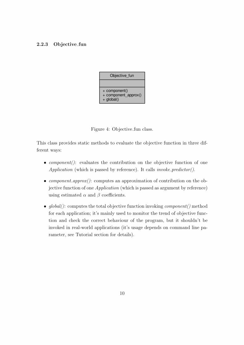
2.2.3 Objective fun
Objective_fun
+ component()+ component_approx()+ global()
Figure 4: Objective fun class.
This class provides static methods to evaluate the objective function in three dif-
ferent ways:
• component(): evaluates the contribution on the objective function of one
Application (which is passed by reference). It calls invoke predictor().
• component approx(): computes an approximation of contribution on the ob-
jective function of one Application (which is passed as argument by reference)
using estimated α and β coefficients.
• global(): computes the total objective function invoking component() method
for each application; it’s mainly used to monitor the trend of objective func-
tion and check the correct behaviour of the program, but it shouldn’t be
invoked in real-world applications (it’s usage depends on command line pa-
rameter, see Tutorial section for details).
10

2.2.4 Bounds
Bounds
+ Bounds()+ calculate_bounds()+ get_app_manager()- bound()- find_bound()
Batch
+ Batch()+ calculate_nu()+ initialize()+ fix_initial_solution()+ write_results()+ show_session_app_id()+ show_bounds()+ show_solution()+ get_begin()+ get_cbegin()+ get_end()+ get_cend()+ get_empty()
-app_manager
std::vector< Application >
-APPs
Application
- ncores_new- R_old- chi_C- m- M- Deadline_d- csi- alpha- beta
+ Application()+ compute_alpha_beta()+ get_session_app_id()+ get_app_id()+ get_w()+ get_term_i()+ get_chi_0()+ get_chi_C()+ get_m()+ get_M()and 23 more...
+elements
double
-R_new-term_i
-ncores_old-v
-nu_d-w-V
-R_d-chi_0
-baseFO...
int
-vm-bound_iterations
-dataset_size-nCores_DB_d
-bound-currentCores_d
std::string
-session_app_id-app_id-stage
std::basic_string< char >
Figure 5: Bounds class.
Bounds class provides calculate bounds() method to evaluate the bounds for the
applications stored in the Batch object i.e. the minimal number of cores necessary
to finish the execution before deadline; it supports openMP. The public member
function calculate bounds() uses the private members functions find bound() and
bound(). Here is a description of methods:
• bound(): it’s a private method. This function calculates the bound for
one application (which is passed by reference) through a hill climbing: in-
voke predictor() function is invoked until an upper bound is found, then a
rollback is performed to return the last ”safe” number of cores and time. At
each iteration the Application::compute alpha beta() method is invoked.
11

• find bound(): it’s a private method. Firstly it finds a guess for the bound for
one application (which is passed by reference): it queries the table OPTI-
MIZER CONFIGURATION TABLE to find the number of cores calculated
by OPT IC earlier (see [1] for details). Secondly, it invokes the bound()
function.
• calculate bound(): evaluates the bound for each application in the Batch
member object. If the number of threads is greater than 0, each Application
is assigned to a thread, a database connection is opened for each thread
and for each Application in the Batch member the findbound() method is
invoked; otherwise the same thing is done sequentially.
• get app manager(): it returns the Batch object.
12
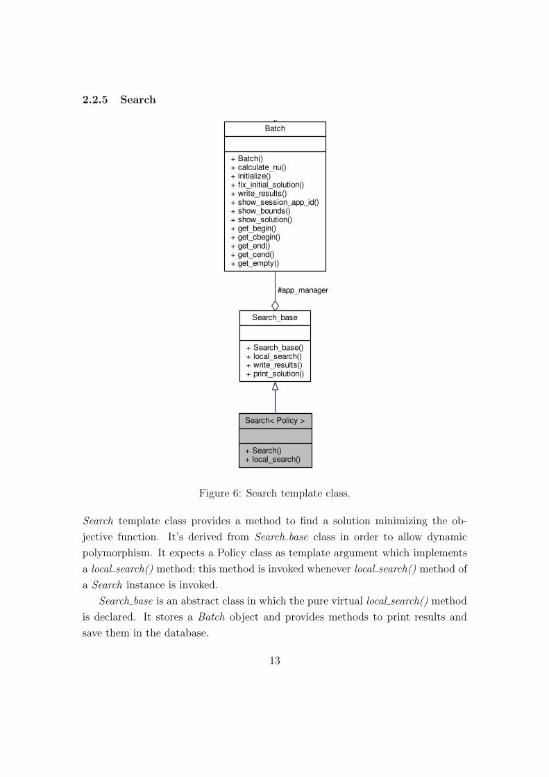
2.2.5 Search
Search< Policy >
+ Search()+ local_search()
Search_base
+ Search_base()+ local_search()+ write_results()+ print_solution()
Batch
+ Batch()+ calculate_nu()+ initialize()+ fix_initial_solution()+ write_results()+ show_session_app_id()+ show_bounds()+ show_solution()+ get_begin()+ get_cbegin()+ get_end()+ get_cend()+ get_empty()
#app_manager
std::vector< Application >
-APPs
Application
- ncores_new- R_old- chi_C- m- M- Deadline_d- csi- alpha- beta
+ Application()+ compute_alpha_beta()+ get_session_app_id()+ get_app_id()+ get_w()+ get_term_i()+ get_chi_0()+ get_chi_C()+ get_m()+ get_M()and 23 more...
+elements
double
-R_new-term_i
-ncores_old-v
-nu_d-w-V
-R_d-chi_0
-baseFO...
int
-vm-bound_iterations
-dataset_size-nCores_DB_d
-bound-currentCores_d
std::string
-session_app_id-app_id-stage
std::basic_string< char >
Figure 6: Search template class.
Search template class provides a method to find a solution minimizing the ob-
jective function. It’s derived from Search base class in order to allow dynamic
polymorphism. It expects a Policy class as template argument which implements
a local search() method; this method is invoked whenever local search() method of
a Search instance is invoked.
Search base is an abstract class in which the pure virtual local search() method
is declared. It stores a Batch object and provides methods to print results and
save them in the database.
13

Search factory class is used to build dinamically a Search instance; the search builder()
method chooses a policy for Search template class according to command line pa-
rameters (see Tutorial section for details) and returns a unique pointer to Search base
class.
2.2.6 Candidates
Candidates
+ add_candidate()+ invoke_predictor_openMP()+ invoke_predictor_seq()+ get_size()+ get_empty()+ get_begin()+ get_cbegin()+ get_end()+ get_cend()
std::list< Candidate_pair >
-cand
Candidate_pair
+ Candidate_pair()+ get_app_id_i()+ get_app_id_j()+ get_session_app_id_i()+ get_session_app_id_j()+ get_delta_fo()+ get_new_core_assignment_i()+ get_new_core_assignment_j()+ get_real_i()+ get_real_j()and 10 more...
+elements
double
-real_i-real_j
-delta_fo
Application
- ncores_new- R_old- chi_C- m- M- Deadline_d- csi- alpha- beta
+ Application()+ compute_alpha_beta()+ get_session_app_id()+ get_app_id()+ get_w()+ get_term_i()+ get_chi_0()+ get_chi_C()+ get_m()+ get_M()and 23 more...
-R_new-term_i
-ncores_old-v
-nu_d-w-V
-R_d-chi_0
-baseFO...
-app_i-app_j
int
-vm-bound_iterations
-dataset_size-nCores_DB_d
-bound-currentCores_d
-delta_i-delta_j
-new_core_assignment_i
-new_core_assignment_j
std::string
-session_app_id-app_id-stage
std::basic_string< char >
Figure 7: Candidates class.
Candidates is an auxiliary class used by local search() methods; it stores a list
of Candidate pair objects. In each Candidate pair are stored data about pairs
14

of applications and the consequent changes on the objective function after cores
exchange.
Candidates stores pairs of applications for which a cores exchange could be
profitable and provides methods to evaluate in parallel or sequentially the objective
function.
Here those methods are described:
• invoke predictor openMP(): calls in parallel the evaluation of the objective
function for each pair of applications and stores the results in real i, real j
(members of Candidate pair). Since some pairs could share the same val-
ues, an auxiliary vector<Application> with unique copies of the applications
is used in order to avoid unnecessary calls and errors while accessing the
database.
Each Application in the auxiliary vector is assigned to a thread, a database
connection is opened for each thread and for each Application in the Batch
member the Objective fun::component() method is invoked. Then results are
stored in the list <Candidate pair> member.
This methods is invoked from Policy methods::exact loop() if the number of
threads is greater than 0.
• invoke predictor seq(): does the same as invoke predictor openMP() but se-
quentially.
15

2.2.7 Policy methods
Figure 8: Policy methods class.
Policy methods class provides useful methods to find a solution minimizing the
objective function; those methods are used by children classes.
Here is a description of them:
• approximated loop(): given a Batch object by reference, it estimates the
objective function for each move i.e. for each pair of applications. The
evaluation is done using α and β coefficients. The pairs of applications for
which the move is profitable - i.e. for which the ∆(objectivefunction) < 0
- are stored ordered by increasing ∆(objectivefunction) in a Candidates
object (which is returned).
• exact loop(): given a Candidates object and a Batch object by reference, it
executes an ”invoke predictor ” method of Candidates ( invoke predictor openMP()
if the number of threads is greater than 0, invoke predictor seq() otherwise).
If there are pairs of Applications for which the exchange is profitable, the
best pair is selected and the exchange is done in the Batch object.
• check total nodes(): checks that the total allocated nodes is still less or equal
than the total number of cores available.
16

2.2.8 Policy alterning
Policy_alterning
+ local_search()
Policy_methods
+ check_total_nodes()+ approximated_loop()+ exact_loop()
Figure 9: Policy alterning class.
Policy alterning is a policy-class: it is passed as template argument to Search in
order to set the local search() method.
The local search() method requires a Batch object as argument and performs a
single loop. At each iteration approximated loop() is invoked and returns a Candi-
dates object (say cand) containing potential profitable moves; then exact loop(Candidates
cand, ...) is invoked, which evaluates the objective function for selected pairs. This
is done until no more profitable exchanges are found or the maximum number of
iterations is reached.
17

2.2.9 Policy separing
Policy_separing
+ local_search()
Policy_methods
+ check_total_nodes()+ approximated_loop()+ exact_loop()
Figure 10: Policy separing class.
Policy separing is a policy-class: it is passed as template argument to Search in
order to set the local search() method.
The local search() method requires a Batch object as argument and performs
two separates loop.
In the first loop, at each iteration, is invoked approximated loop() which returns
a Candidates object containing potential profitable moves; then the most profitable
move (the first since the list in Candidates is ordered by ∆(objectivefunction)) is
done in the Batch object. The loop ends when there are no more profitable moves
or (rather improbably) the maximum number of iterations is reached.
In the second loop, at each iteration, first a Candidates object with all pos-
sible exchanges of cores between applications is built (say all cand), then ex-
act loop(Candidates all cand, ...) is invoked, which evaluates the objective func-
tion for all possible pairs. The loop ends when there are no more profitable moves
or the maximum number of iterations is reached.
Note that using this policy the auxiliary vector used in Candidates::invoke predictor openMP()
18

is fundamental since almost surely there are repetitions of applications in the Can-
didates object.
2.2.10 Other Classes
A short description of minor classes is reported here below.
• Configuration: stores data from the wsi config.xml file in an unordered map<
string, string >; it overloads the [] operator to allow easy access to the map.
• Opt jr parameters : stores parameters received from command line, which
are visible with getter functions.
• Statistics : if global evaluation of objective function is activated (see Tutorial
section for details), this class stores a vector of Statistic iter objects; each
Statistic iter includes relevant statistical information about a single iteration
in local search().
19

3 Numerical Results
In this section performances on objective function and time of execution of the
OPT JR CPP program are discussed. Time performances have been measured on
a 8-cores machine located at the DEIB.
Here is reported the graph of the objective function at each local search() iter-
ation using the Alterning policy. The test has been done using 4 applications, 150
available cores, 15 maximum iterations and no limits to the maximum number of
considered candidates.
Figure 11: OF evaluation at each iteration, 4 applications, Alterning.
The graph shows that the solution improves rather quickly and it stops after
just 2 iterations; this is not surprising since the initial solution should be a good
guess.
20
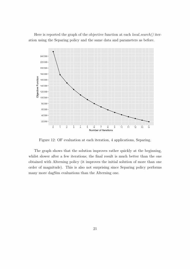
Here is reported the graph of the objective function at each local search() iter-
ation using the Separing policy and the same data and parameters as before.
Figure 12: OF evaluation at each iteration, 4 applications, Separing.
The graph shows that the solution improves rather quickly at the beginning,
whilst slower after a few iterations; the final result is much better than the one
obtained with Alterning policy (it improves the initial solution of more than one
order of magnitude). This is also not surprising since Separing policy performs
many more dagSim evaluations than the Alterning one.
21

Here is reported the graph of the objective function at each local search() iter-
ation using the Alterning policy. The test has been done using 8 applications and
others parameters as before.
Figure 13: OF evaluation at each iteration, 8 applications, Alterning.
Again the improvements are rather fast and the solution is found after a few
iterations.
22

Here is reported the graph of the objective function at each local search() it-
eration using the Separing policy. The test has been done using 8 applications,
parameters as above.
Figure 14: OF evaluation at each iteration, 8 applications, Separing.
Again the solution improves rather quickly at the beginning, slower after a few
iterations, but the result is much better than the one obtained with Alterning
policy.
23

Time performance is discussed henceforward; this analysis wants to show time-
improvements given by parallelization (on a multi-core machine). The analysis is
divided in two sections corresponding to the two adopted policies. Each section is
divided in subsections corresponding to the state of the cache i.e. to the percentage
of data to evaluate which are already located in the database. This distinction is
fundamental since the predictor dagSim (which is quite slow, about 2.5 minutes
for a single call) is not executed if the result is already stored.
In case of full cache (i.e. dagSim is never invoked) total execution time is
so small (under 0.1 seconds) that the time difference using multiple threads is
negligible; the same happens for both the policies for any number of applications.
Much more intersting are the cases in which the cache is not full, which are
described in the next pages.
24

3.1 Policy alterning
Time performances of the Alterning policy are described below.
Cache off
Tests on this section have been done with cache disabled; note that this
scenario is even worse than the worst scenario possible, since not only the
cache is empty but there could be some repetitions when invoking dagSim.
Here are reported results on a test with 4 application, 150 available cores,
10 maximum iterations and no limits to the maximum number of consid-
ered candidates; time measurements are reported by varying the number of
threads.
Figure 15: Time performance, cache off, 4 applications, Alterning.
We note that total execution time improves up to 4 threads, then stabilizes.
The sequencial version spends about 27 minutes to complete the execution
while the parallel version with 4 cores spends less than 10 minutes. This
corresponds to a 63% improvement.
25

Here are reported results on a test with 8 application, 150 available cores,
10 maximum iterations and no limits to the maximum number of consid-
ered candidates; time measurements are reported by varying the number of
threads.
Figure 16: Time performance, cache off, 8 applications, Alterning.
We note that the total execution time continues to improve increasing the
number of threads. The sequencial version spends about 1 hour and 8 min-
utes to complete the execution while the parallel version with 8 cores spends
less than 15 minutes. This corresponds to a 78% improvement.
26

Cache 50%
Tests on this section have been done with cache 50% full, which could rep-
resent a real world scenario.
Here are reported results on a test with 4 application, 150 available cores,
10 maximum iterations and no limits to the maximum number of consid-
ered candidates; time measurements are reported by varying the number of
threads.
Figure 17: Time performance, 50% cache, 4 applications, Alterning.
The sequencial version spends about 12 minutes to complete the execution
while the parallel version with 4 cores spends less than 8 minutes. This
corresponds to a 33% improvement.
3.2 Policy separing
Here time performances of the Separing policy are described. Since the Separing
policy is rather slow, it has been tested only with four applications.
27

Cache 0%
Since there are many repetitions in invoking dagSim, turning off the cache
leads to very long times (about 41 minutes with 4 cores and 4 applications).
To represent the worst scenario is more meaningful to turn on the cache and
start from an empty database.
Here are reported results on a test with 4 application, 150 available cores,
10 maximum iterations and no limits to the maximum number of consid-
ered candidates; time measurements are reported by varying the number of
threads.
Figure 18: Time performance, 0% cache, 4 applications, Separing.
The sequencial version spends about 60 minutes to complete the execution
while the parallel version with 8 cores spends less than 25 minutes. This
corresponds to a 58% improvement.
28

Cache 50%
Tests on this section have been done with cache 50% full, which could rep-
resent a real world scenario.
Here are reported results on a test with 4 application, 150 available cores,
10 maximum iterations and no limits to the maximum number of consid-
ered candidates; time measurements are reported by varying the number of
threads.
Figure 19: Time performance, 50 % cache, 4 applications, Separing.
The sequencial version spends about 30 minutes to complete the execution
while the parallel version with 8 cores spends about 17.5 minutes. This
corresponds to a 41% improvement.
29

4 Conclusion
Both local search policies lead to remarkable improvements of the initial solution
in the objective function; the improvements are greater when using the Separing
policy.
The parallelization leads to a big decrease on execution time and indeed it has
already been adopted from the original C program. We observed improvements
from 33% to 78% in total execution time using Alterning policy and from 41% to
58% using Separing policy.
We observe that time improvement decreases as the percentage of already com-
puted predictions increases.
Separing policy is generally slow, so it should be used if the number of appli-
cation is small and the percentage of already computed values is expected to be
high.
Policy alterning is quite fast; with parallelization and a small amount of al-
ready computed values it should meet the ideal deadline of 10 minutes; however
the maximum number of iterations and the limit on the maximum number of con-
sidered candidates (see Tutorial section for details) could be set in order to meet
the deadline.
The policy structure of the program allows an easy extension of the program;
indeed if another type of local search has to be implemented it could be done
with a policy class implementing a local search() method. For istance, a local
search doing multiple virtual machines exchanges could be done, or the search
could explore the neighborood more deeply allowing cores exchange between more
than two applications at each iteration.
30

5 Tutorial
Here is reported a tutorial on the usage of the program as described in the
README file at https://github.com/davide-burba/PACS PROJECT.
USAGE:
./OPT JR CPP -f< filename.csv > -n< N > -k< Limit > -d< Y/y|N/n >-c< Y/y|N/n > -g=< Y/y|N/n > -i< iterations > -st< a/A|s/S >
where:
< filename.csv > is the csv file defining the profile applications under $UP-
LOAD HOME in wsi config.xml;
< N > is the total number of cores;
< Limit > is the maximum number of considered candidates (if equal to 0, all
the candidates are considered).
-d represents debug (on/off)
-c represents cache (on/off)
-g prints the value of the global objective function (on/off)
-i represents the maximum number of iterations
-st represents the type of local search: a/A alternates approximate evaluation
of objective function with dagSim evaluation, while s/S performs separately an
approximate loop and a dagSim loop. If -st=s/S -k should be set to 0.
References
[1] Danilo Ardagna, Enrico Barbierato (Polimi); Jussara M. Almeida, Ana Paula
Couto Silva (UFMG) (2016). D3.2 - Big Data Application Performance
models and run-time Optimization Policies www.eubra-bigsea.eu
31