Embed Size (px)
Citation preview
POLITECNICO DI MILANOCorso di Laurea Magistrale in Ingegneria Biomedica
Scuola di Ingegneria Industriale e dell’Informazione
Dipartimento di Elettronica, Informazione e Bioingegneria
Tesi di Laurea Magistrale
MECHANICS OF ARTICULAR CARTILAGE: DERIVATION AND
NUMERICAL IMPLEMENTATION OF A VISCOELASTIC MODEL
WITH STATISTICAL FIBRE DISTRIBUTION
Relatore: Prof. Pasquale VENA
Autore:
Gianluca GABELLINI
Matricola n. 765583
ANNO ACCADEMICO 2012–2013
Viscoelastic modelling of articular cartilage
Gianluca Gabellini
Supervisor: T. Christian Gasser, Ph.D.
Master’s Degree Project
Stockholm, Sweden 2013
KTH School of Engineering Sciences
Department of Solid Mechanics
Royal Institute of Technology
SE-100 44 Stockholm - Sweden

To my parents
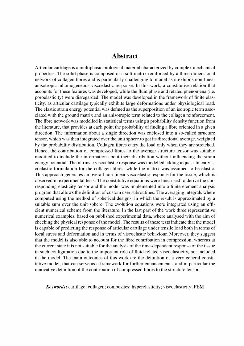
AbstractArticular cartilage is a multiphasic biological material characterized by complex mechanicalproperties. The solid phase is composed of a soft matrix reinforced by a three-dimensionalnetwork of collagen fibres and is particularly challenging to model as it exhibits non-linearanisotropic inhomogeneous viscoelastic response. In this work, a constitutive relation thataccounts for these features was developed, while the fluid phase and related phenomena (i.e.poroelasticity) were disregarded. The model was developed in the framework of finite elas-ticity, as articular cartilage typically exhibits large deformations under physiological load.The elastic strain energy potential was defined as the superposition of an isotropic term asso-ciated with the ground matrix and an anisotropic term related to the collagen reinforcement.The fibre network was modelled in statistical terms using a probability density function fromthe literature, that provides at each point the probability of finding a fibre oriented in a givendirection. The information about a single direction was enclosed into a so-called structuretensor, which was then integrated over the unit sphere to get its directional average, weightedby the probability distribution. Collagen fibres carry the load only when they are stretched.Hence, the contribution of compressed fibres to the average structure tensor was suitablymodified to include the information about their distribution without influencing the strainenergy potential. The intrinsic viscoelastic response was modelled adding a quasi-linear vis-coelastic formulation for the collagen fibres, while the matrix was assumed to be elastic.This approach generates an overall non-linear viscoelastic response for the tissue, which isobserved in experimental tests. The constitutive equations were linearised to derive the cor-responding elasticity tensor and the model was implemented into a finite element analysisprogram that allows the definition of custom user subroutines. The averaging integrals wherecomputed using the method of spherical designs, in which the result is approximated by asuitable sum over the unit sphere. The evolution equations were integrated using an effi-cient numerical scheme from the literature. In the last part of the work three representativenumerical examples, based on published experimental data, where analysed with the aim ofchecking the physical response of the model. The results of these tests indicate that the modelis capable of predicting the response of articular cartilage under tensile load both in terms oflocal stress and deformation and in terms of viscoelastic behaviour. Moreover, they suggestthat the model is also able to account for the fibre contribution in compression, whereas atthe current state it is not suitable for the analysis of the time-dependent response of the tissuein such configuration due to the important role of fluid-related viscoelasticity, not includedin the model. The main outcomes of this work are the definition of a very general consti-tutive model, that can serve as a framework for further enhancements, and in particular theinnovative definition of the contribution of compressed fibres to the structure tensor.
Keywords: cartilage; collagen; composites; hyperelasticity; viscoelasticity; FEM

Acknowledgments
First, I would like to acknowledge my supervisor at KTH Christian Gasser. He was an in-
spiration, a guide and a priceless source of help throughout my project. I would also like to
thank professor Pasquale Vena for his valuable suggestions and his support during all the
stages of this work.
Last but not least, I would like to thank my parents for the unconditional support and the
constant encouragement that made this possible.
Gianluca Gabellini
Milano, April 2014
v
Contents
Sommario 1
1 Introduction 11
1.1 Problem background . . . . . . . . . . . . . . . . . . . . . . . . . . . . . 11
1.2 Mechanical properties of articular cartilage . . . . . . . . . . . . . . . . . 13
1.3 Constitutive modelling of articular cartilage . . . . . . . . . . . . . . . . . 16
1.4 Objective . . . . . . . . . . . . . . . . . . . . . . . . . . . . . . . . . . . 18
2 Continuum mechanical framework 19
2.1 Motion and deformation gradient . . . . . . . . . . . . . . . . . . . . . . . 19
2.2 Strain measures . . . . . . . . . . . . . . . . . . . . . . . . . . . . . . . . 21
2.3 Stress measures . . . . . . . . . . . . . . . . . . . . . . . . . . . . . . . . 23
2.4 Hyperelastic materials . . . . . . . . . . . . . . . . . . . . . . . . . . . . 25
2.4.1 Incompressible hyperelastic materials . . . . . . . . . . . . . . . . 26
2.4.2 Isotropic hyperelastic materials . . . . . . . . . . . . . . . . . . . 28
2.4.3 Fibre reinforced hyperelastic materials . . . . . . . . . . . . . . . . 29
2.5 Viscoelasticity at finite deformation . . . . . . . . . . . . . . . . . . . . . 30
2.6 Elasticity tensor . . . . . . . . . . . . . . . . . . . . . . . . . . . . . . . . 33
3 Methods 36
3.1 Structure tensor . . . . . . . . . . . . . . . . . . . . . . . . . . . . . . . . 36
3.2 Anisotropic viscoelastic formulation at finite strains . . . . . . . . . . . . . 38
3.2.1 Modified structure tensor . . . . . . . . . . . . . . . . . . . . . . . 41
3.2.2 Viscoelastic contribution . . . . . . . . . . . . . . . . . . . . . . . 46
3.3 Illustrative fibre distribution . . . . . . . . . . . . . . . . . . . . . . . . . 48
3.4 Spatial isochoric structure tensor . . . . . . . . . . . . . . . . . . . . . . . 50
vi
CONTENTS vii
3.5 Cauchy stress tensor and spatial elasticity tensor . . . . . . . . . . . . . . . 51
3.6 Numerical implementation . . . . . . . . . . . . . . . . . . . . . . . . . . 54
3.6.1 Structure tensor . . . . . . . . . . . . . . . . . . . . . . . . . . . . 54
3.6.2 Spherical integration . . . . . . . . . . . . . . . . . . . . . . . . . 55
3.6.3 Numerical integration of the evolution equation . . . . . . . . . . . 57
3.7 Representative numerical examples . . . . . . . . . . . . . . . . . . . . . . 60
3.7.1 Incompressibility constraint . . . . . . . . . . . . . . . . . . . . . 61
3.7.2 Solution procedure . . . . . . . . . . . . . . . . . . . . . . . . . . 63
3.7.3 Problems specification . . . . . . . . . . . . . . . . . . . . . . . . 65
4 Results 69
4.1 Relaxation tests . . . . . . . . . . . . . . . . . . . . . . . . . . . . . . . . 69
4.2 Unconfined compression of full thickness specimen . . . . . . . . . . . . . 72
4.3 Unconfined compression of reduced thickness specimen . . . . . . . . . . 74
5 Conclusions 78
References 82
List of Figures
1.1 Representation of articular cartilage in the knee joint. Adapted from [42]. . 12
1.2 Severe articular cartilage damage on a medial femoral condyle (left) and
ineffective formation of scar tissue in a damaged area (right). . . . . . . . . 13
1.3 Representation of the AC layers and fibre orientations through the thickness. 15
3.1 Representation of the unit sphere and the typical pyramidal element and char-
acterization of an arbitrary unit direction vector M in polar coordinates. The
fibres distribution can be seen as a smaller pyramidal element whose base is
determined by ρ(M) as a fraction of dA = sin ΘdΘdΦ. . . . . . . . . . . . 38
3.2 If compressed fibres are simply disregarded IM4 is not a continuous function
of λM (left). The proposed definition of IM4 ensures continuity (right). The
dotted lines represent the original definition of the structure tensor. . . . . . 42
3.3 Cube of incompressible hyperelastic material reinforced by a three dimen-
sional fibre network under tension (left); one-dimensional representation of
stretch level in the fibres (right). . . . . . . . . . . . . . . . . . . . . . . . 43
3.4 Three-dimensional graphical representation of the orientation of collagen fi-
bres based on the transversely isotropic density functions ρA and ρB. Sur-
face plots are defined by the vector ρ(Θ)M, where ρ is given by (3.34a) for
model (A) and by (3.34b) for model (B). Image reproduced from [9]. . . . 49
3.5 Graphical representation of the spherical t-design with t = 21, correspond-
ing to 240 points on the unit sphere. . . . . . . . . . . . . . . . . . . . . . 56
3.6 Flowchart of the solution procedure adopted for the numerical example. . . 64
3.7 Geometry and load for the relaxation tests on full thickness specimen with
layer of subchondral bone. . . . . . . . . . . . . . . . . . . . . . . . . . . 65
3.8 Geometry and load for the unconfined compression of full thickness speci-
men with layer of subchondral bone. . . . . . . . . . . . . . . . . . . . . . 66
viii
LIST OF FIGURES ix
3.9 Geometry and load for the unconfined compression of reduced thickness
specimen. . . . . . . . . . . . . . . . . . . . . . . . . . . . . . . . . . . . 67
4.1 Simulation of a two-steps relaxation test of a full-thickness specimen of AC
in tension and compression using the model. The results are given as external
load vs time. . . . . . . . . . . . . . . . . . . . . . . . . . . . . . . . . . 69
4.2 Comparison between model prediction and experimental data reported in
[35] for both tensile (a) and compressive (b) relaxation tests. The results are
given as axial engineering stress vs time. . . . . . . . . . . . . . . . . . . 70
4.3 (a) Time evolution of normalized axial nominal stress for two tensile relax-
ation tests with different maximum displacement. (b) A QLV fit (dashed line)
based on a power law fit (dotted line) of the results at low strain cannot re-
produce stress relaxation at higher level of strain. The axes are in logarithmic
scale. . . . . . . . . . . . . . . . . . . . . . . . . . . . . . . . . . . . . . 71
4.4 Axial Cauchy stress distribution in deformed specimen at the end of the re-
laxation test (t = 1200s) for tension (a) and compression(b). . . . . . . . . 72
4.5 Load vs displacement for the unconfined compression of a full-thickness
specimen of AC. . . . . . . . . . . . . . . . . . . . . . . . . . . . . . . . 73
4.6 Distribution of first, second and third principal Cauchy stresses in a full-
thickness cylindrical AC specimen under unconfined compression at maxi-
mum displacement u = 0.35mm. The articular surface is the upper surface,
and the lower surface is attached to a layer of subchondral bone. . . . . . . 74
4.7 Load cycle versus displacement for the unconfined compression of a reduced
thickness specimen of AC at two loading frequencies. . . . . . . . . . . . 75
4.8 Distribution of the first, second and third principal Cauchy stresses in a cylin-
drical AC specimen under unconfined compression. Upper (articular) and
lower surfaces are both unconstrained in the radial direction. . . . . . . . . 76
4.9 Dynamic modulus ∂σz∂λz
versus Cauchy normal stress σz . . . . . . . . . . . 76
Sommario
La cartilagine articolare (CA) è un strato relativamente sottile di tessuto connettivo che rico-
pre le superfici di contatto delle ossa nelle articolazioni. Le sue funzioni principali sono la
riduzione dell’attrito e la trasmissione del carico, ma allo stesso tempo agisce come ammor-
tizzatore e distribuisce i carichi su una superficie relativamente ampia prevenendo pericolose
concentrazioni di sforzo.
La CA viene facilmente danneggiata in seguito a traumi o semplicemente a causa dell’usura
nel tempo. Un’area lesionata viene solitamente sostituita da tessuto cicatriziale perché la CA
fatica a rigenerarsi: le cellule non sono libere di migrare nella zona danneggiata e la man-
canza di vascolarizzazione ne rallenta il metabolismo. L’artrosi, una malattia cronica che
causa una perdita progressiva di tessuto cartilagineo, è divenuta la più alta spesa sanitaria
negli Stati Uniti anche a causa dell’invecchiamento della popolazione [8]. Le procedure cli-
niche adottate comunemente vanno dal trattamento conservativo alla rimozione chirurgica di
tessuto danneggiato, ma a lungo termine è solitamente necessario applicare una protesi [16].
Negli ultimi anni è stato proposto di utilizzare tessuto ingegnerizzato cresciuto in laboratorio.
Sebbene promettente, questa soluzione richiede che CA ingegnerizzata e naturale abbiano le
stesse proprietà meccaniche per evitare la comparsa di carichi non fisiologici potenzialmente
pericolosi per il tessuto sano che circonda l’impianto. Per assicurarsi che questo avvenga, è
necessario affiancare alle analisi sperimentali modelli costitutivi come quello presentato in
questo lavoro. Data la complessità della CA infatti i test sperimentali non sono da soli suffi-
cienti per lo studio della relazione tra struttura e funzione [29].
Dal punto di vista meccanico la CA è un materiale poroso composto da una matrice solida
rinforzata da collagene e da una fase liquida. Il movimento del fluido interstiziale attraver-
so la matrice porosa causa dissipazione d’energia. Tale fenomeno, definito viscoelasticità
estrinseca, è solitamente trascurabile in tensione [35]. Questo lavoro si concentra sulla fase
solida della CA e di conseguenza la fase liquida viene trascurata, sebbene influenzi il com-
1
SOMMARIO 2
portamento del tessuto in compressione. Il collagene è organizzato in una complessa rete
tridimensionale di fibre. Il comportamento del tessuto è determinato non solo dalle proprietà
meccaniche di tali fibre ma anche dalla loro disposizione [37]. In particolare si individuano
tre zone principali lungo lo spessore della CA: superficiale, centrale e profonda [40]. Nel-
la prima le fibre sono disposte in prevalenza parallelamente alla superficie articolare; nella
zona intermedia la distribuzione è casuale; nella zona profonda le fibre sono principalmen-
te perpendicolari all’interfaccia con l’osso sottostante. Il collagene è responsabile anche di
quella che viene definita viscoelasticità intrinseca (chiamata semplicemente viscoelasticità
nel seguito), la quale determina il comportamento tempo-dipendente del tessuto in trazione.
Numerosi modelli analitici e numerici sono stati proposti per la CA. Le elevate deformazioni
a cui è sottoposto il tessuto sotto carichi fisiologici rende in primo luogo necessaria una trat-
tazione in grandi deformazioni [9] [32]. La fase solida è stata modellata sia come continuo
[31] sia a partire dai costituenti [9] [32]. In generale il secondo approccio garantisce una
migliore rappresentazione del rinforzo fibroso e del suo contributo. Similmente la viscoela-
sticità delle fibre di collagene è stata modellata con formulazioni lineari [57], quasi-lineari
[26] e non lineari [43]. In particolare la formulazione quasi-lineare rappresenta una scelta
comune in letteratura per i tessuti biologici con rinforzati da collagene [21] [62] e specifica-
mente per la CA [32].
In questo contesto il presente lavoro ha come obiettivo generale la definizione di un mo-
dello costitutivo di tipo continuo per la fase solida della CA che sia in grado di riprodur-
ne le proprietà anisotrope e non omogenee e le caratteristiche tempo-dipendenti, che possa
essere integrato con modelli per la fase liquida. I tre obiettivi specifici sono la definizio-
ne di una quantità strutturale che tenga conto della distribuzione del collagene nel tessuto,
l’introduzione di formulazione viscoelastica valida intorno all’equilibrio termodinamico e
l’implementazione del corrispondente modello numerico.
Modello costitutivo
I tessuti biologici rinforzati da collagene possono essere trattati con una formulazione basata
sugli invarianti della deformazione e sulla sovrapposizione di un potenziale isotropo associa-
to alla matrice e uno trasversalmente isotropo associato alle fibre. Le fibre vengono suddivise
in famiglie e le informazioni sulla direzione di ciascuna di esse vengono racchiuse in un co-
SOMMARIO 3
siddetto tensore strutturale [25]. Tuttavia la complessa rete tridimensionale di collagene che
caratterizza la CA può essere modellata più efficacemente come un’unica famiglia di fibre
statisticamente distribuita intorno ad un asse polare. A questo scopo è stato proposto in [13]
di ridefinire il tensore strutturale calcolandone una media direzionale sulla sfera unitaria,
approccio adottato in questo lavoro.
Il tensore tensore strutturale assume la seguente espressione:
H =1
4π
∫ 2π
0
∫ π
0
ρ(Θ)M(Θ,Φ)⊗M(Θ,Φ) sin Θ dΘ dΦ =1
4π
∫S2
ρ(M)A(M) dS
dove A(M) = M⊗M è il contributo al tensore strutturale associato alla direzione M e ρ
è la funzione di probabilità che caratterizza la distribuzione di fibre nella configurazione a
riposo. In accordo con [13] è stata scelta una distribuzione trasversalmente isotropa attorno
al proprio asse polare, sufficiente a rappresentare la disposizione delle fibre nelle tre zone in
cui viene suddivisa la CA.
La configurazione iniziale è stata considerata priva di sforzi e il tessuto incomprimibile. Que-
st’ipotesi rende necessaria la definizione della sola parte deviatorica del potenziale, in quanto
la parte volumetrica è determinata a partire dalle condizioni al contorno. Il potenziale devia-
torico è determinato da un contributo legato alla matrice e da uno legato alle fibre. In accordo
con molti lavori in letteratura [24] [13] [1], la matrice è stata rappresentata per semplicità co-
me materiale neo-hookeano isotropo. Il potenziale delle fibre è invece stato suddiviso in un
contributo isotropo che tiene conto delle diverse proprietà meccaniche rispetto alla matrice,
ed uno anisotropo che rappresenta le proprietà trasversalmente isotrope delle fibre. Per il
primo è stato nuovamente scelto un modello neo-hookeano con parametri diversi da quelli
della matrice; il secondo incorpora le informazioni sulle fibre attraverso il tensore strutturale
definito in precedenza:
Ψ∞fa(C,H) =1
2cfa(H : C− 1)2 =
1
2cfa(I4 − 1)2
dove cfa è una costante, C è la parte deviatorica tensore di deformazione di Cauchy-Green e
I4 è un invariante di tale tensore e rappresenta l’allungamento medio delle fibre nel punto in
cui il potenziale viene calcolato.
La scelta di un legame quadratico ha lo scopo di replicare un fenomeno tipico dei tessu-
ti biologici definito reclutamento: le fibre di collagene sono ondulate a riposo e il carico
necessario a distenderle è trascurabile rispetto a quello che trasmettono una volta orientate
SOMMARIO 4
nella direzione della sollecitazione. Questo si traduce in un incremento di pendenza nella
curva carico-deformazione che può essere modellato efficacemente per mezzo di un legame
non-lineare. In particolare è riportato in letteratura che un polinomio di secondo ordine è in
generale sufficiente a riprodurre il comportamento del tessuto in casi d interesse, come ad
esempio quello della cartilagine ingegnerizzata, la quale non presenta forti non linearità in
grandi deformazioni [51].
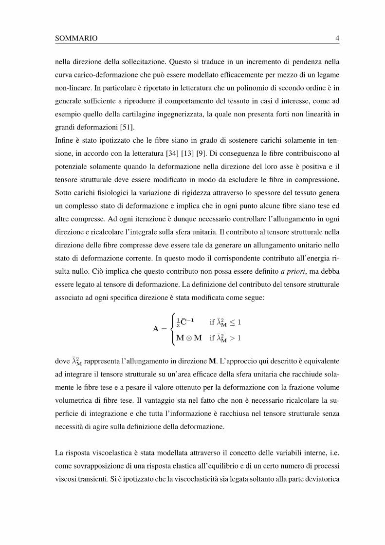
Infine è stato ipotizzato che le fibre siano in grado di sostenere carichi solamente in ten-
sione, in accordo con la letteratura [34] [13] [9]. Di conseguenza le fibre contribuiscono al
potenziale solamente quando la deformazione nella direzione del loro asse è positiva e il
tensore strutturale deve essere modificato in modo da escludere le fibre in compressione.
Sotto carichi fisiologici la variazione di rigidezza attraverso lo spessore del tessuto genera
un complesso stato di deformazione e implica che in ogni punto alcune fibre siano tese ed
altre compresse. Ad ogni iterazione è dunque necessario controllare l’allungamento in ogni
direzione e ricalcolare l’integrale sulla sfera unitaria. Il contributo al tensore strutturale nella
direzione delle fibre compresse deve essere tale da generare un allungamento unitario nello
stato di deformazione corrente. In questo modo il corrispondente contributo all’energia ri-
sulta nullo. Ciò implica che questo contributo non possa essere definito a priori, ma debba
essere legato al tensore di deformazione. La definizione del contributo del tensore strutturale
associato ad ogni specifica direzione è stata modificata come segue:
A =
13C−1 if λ2
M ≤ 1
M⊗M if λ2M > 1
dove λ2M rappresenta l’allungamento in direzione M. L’approccio qui descritto è equivalente
ad integrare il tensore strutturale su un’area efficace della sfera unitaria che racchiude sola-
mente le fibre tese e a pesare il valore ottenuto per la deformazione con la frazione volume
volumetrica di fibre tese. Il vantaggio sta nel fatto che non è necessario ricalcolare la su-
perficie di integrazione e che tutta l’informazione è racchiusa nel tensore strutturale senza
necessità di agire sulla definizione della deformazione.
La risposta viscoelastica è stata modellata attraverso il concetto delle variabili interne, i.e.
come sovrapposizione di una risposta elastica all’equilibrio e di un certo numero di processi
viscosi transienti. Si è ipotizzato che la viscoelasticità sia legata soltanto alla parte deviatorica
SOMMARIO 5
della deformazione in accordo con la letteratura [25]. Inoltre nel modello solo le fibre di
collagene sono viscoelastiche, mentre i proteoglicani sono elastici. Questa scelta si basa
sull’evidenza sperimentale che la CA mostra un marcato comportamento viscoelastico anche
in tensione, dove il contributo del fluido e dei proteglicani è trascurabile [34]. In accordo
con le ipotesi riportate, ed esprimendo il contributo viscoso in funzione di quello elastico
all’equilibrio, la forma completa del potenziale deviatorico è la seguente
Ψ = Ψg(C) + (1 +m∑α=1
β∞α )[Ψ∞fi (C) + Ψ∞fa(C,H)]
dove Ψg e Ψ∞fi rappresentano il contributo neo-hookean legato rispettivamente a matrice e
fibre, mentre le costanti adimensionali β∞α ∈ [0,∞) legano la rappresentazione elastica e
quella viscosa. Tale approccio è valido intorno all’equilibrio termodinamico. La relazione
sopra riportata estende la viscoelasticità lineare al campo delle grandi deformazioni tenendo
conto della legame non lineare tra sforzo e deformazione. Ciascun elemento della somma-
toria corrisponde nel caso lineare al contributo di un singolo elemento in un modello di
Maxwell generalizzato. In questo modo si tiene conto del fatto che il rilassamento non av-
viene in un unico istante ma in un intervallo di tempo. È possibile definire tanti processi
di rilassamento quanti necessari per riprodurre accuratamente il comportamento di un ma-
teriale. In questo lavoro sono stati definiti tre elementi, essendo riportato in letteratura che
questo è sufficiente per approssimare correttamente il comportamento della CA [35] [58]. La
relazione usata per le fibre di collagene è di tipo quasi-lineare. Questo implica che in un test
di rilassamento degli sforzi la funzione di rilassamento (ovvero lo sforzo normalizzato sullo
sforzo massimo al termine della rampa di carico) è indipendente dal livello di deformazione
applicato. Sperimentalmente è stato dimostrato che questo non avviene nel caso della CA
[2]. Tuttavia, la sovrapposizione di una matrice elastica e di un rinforzo viscoelastico quasi-
lineare genera un comportamento tempo-dipendente globalmente non lineare per il tessuto,
come già indicato in [62]. A bassi livelli di deformazione, dove la risposta è dominata dalla
matrice, l’effetto viscoso è limitato. Quest’ultimo aumenta progressivamente verso livelli di
deformazione maggiori dove più fibre sono attive e il carico è sostenuto prevalentemente
dalle fibre di collagene.
SOMMARIO 6
Implementazione numerica
Data la complessità di geometrie, proprietà del tessuto e condizioni di carico, non è in ge-
nerale possibile calcolare una soluzione analitica per il modello qui presentato ed è perciò
necessario introdurre dei metodi di soluzione numerici. Il metodo degli Elementi Finiti ha
dimostrato di essere particolarmente efficace nella modellazione di tessuti biologici ed è co-
munemente utilizzato in letteratura. Il legame costitutivo è stato dunque implementato in
linguaggio FORTRAN e aggiunto come subroutine in un software di simulazione tramite il
quale è poi stata eseguita l’analisi ad Elementi Finiti.
La soluzione delle equazioni costitutive viene calcolata in configurazione deformata. Sono
dunque state derivate le corrispondenti espressioni per il tensore strutturale e per gli sforzi
generati dalla particolare espressione scelta per il potenziale. Inoltre la soluzione del sistema
di equazioni differenziali che governa il modello viene calcolata applicando metodi numerici
iterativi e risolvendo una sequenza di problemi lineari. Dato che il modello opera nel campo
delle grandi deformazioni, questo ha richiesto la linearizzazione del legame tra sforzo e de-
formazione e la definizione del corrispondente tensore di elasticità. Inoltre la deformazione
viene ricalcolata ad ogni iterazione, perciò il numero e la direzione delle fibre tese (i.e. at-
tive) può variare durante il processo di riduzione dell’errore, andando di fatto a modificare
la soluzione esatta. Questo aumenta il tempo di calcolo e può causare problemi di conver-
genza. Per questa ragione il valore dell’allungamento calcolato all’istante precedente è stato
utilizzato durante tutte le iterazioni, assumendo che le variazioni di tempo e carico siano
sufficientemente piccole da rendere la differenza trascurabile.
Il tensore strutturale viene integrato sfruttando un efficiente algoritmo suggerito in [9], ba-
sato sul cosiddetto t-design, che definisce il sottoinsieme di punti sulla sfera unitaria in cui
l’integrale viene valutato. Il numero e la posizione dei punti cambia in funzione del grado
di precisione richiesto che è a sua volta funzione della distribuzione scelta per rappresentare
le fibre. Una serie di test numerici di compressione sono stati utilizzati per determinare il
minimo grado t che garantisce convergenza. È infatti importante limitare l’ordine di integra-
zione in quanto un suo aumento incrementa sensibilmente la dimensione del problema e la
quantità di memoria richiesta alla macchina su cui è eseguita l’analisi.
L’algoritmo di discretizzazione dell’integrale di convoluzione che definisce il contributo vi-
scoso e di aggiornamento di sforzi e tensore elastico è basato su un approccio consolidato in
letteratura per la viscoelasticità in grandi deformazioni [60] [21] [14].
Il modello è stato implementato secondo un approccio variazionale misto, che definisce ap-
SOMMARIO 7
prossimazioni separate per pressione e deformazione volumetrica evitando di incorrere in
problemi numerici causati dall’ipotesi di incomprimibilità. Inoltre l’applicazione del metodo
dei lagrangiani aumentati garantisce che il processo di soluzione venga iterato finché l’ipotesi
di incomprimibilità non è correttamente rispettata.
Risultati
Il modello è stato utilizzato per riprodurre dei test sperimentali di rilassamento dello sforzo in
tensione e compressione descritti in [35]. I risultati mostrano un’asimmetria tra le due prove,
dovuta al maggior contributo del collagene in trazione e in accordo con evidenze sperimen-
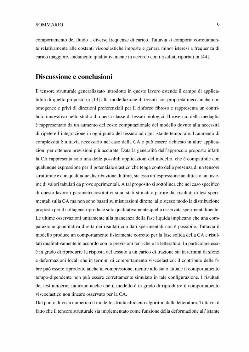
tali. Per quanto riguarda la trazione, la previsione del modello è in perfetto accordo con i dati
riportati in [35] sia per quanto riguarda i valori di sforzo che l’evoluzione del rilassamento,
come mostrato in figura 1a. In compressione invece il modello produce un valore di sforzo al-
l’equilibrio leggermente maggiore di quanto misurato sperimentalmente, mentre sottostima
la componente viscosa che nei dati sperimentali tiene conto anche del contributo del fluido. I
risultati indicano comunque che il contributo delle fibre in compressione non può essere tra-
scurato. Tale contributo appare tuttavia sovrastimato nel modello, il che può essere attribuito
almeno in parte alla distribuzione scelta per rappresentare il collagene. Essa infatti definisce
una zona superficiale (in cui le fibre sono attivate in compressione dall’effetto di Poisson) più
spessa di quella che si osserva nel tessuto reale. Una prova di rilassamento caratterizzata da
una deformazione applicata maggiore dimostra invece la non linearità viscoelastica del mo-
dello. In figura 1b la funzione di rilassamento cambia al variare dello spostamento massimo
applicato, mentre la risposta viscoelastica lineare è per definizione indipendente dal livello
di deformazione.
Un secondo test analizza l’effetto delle fibre sotto carico di compressione. I risultati mo-
strano innanzi tutto un andamento quadratico dello sforzo che può essere addebitato ad un
sostanziale contributo delle fibre, dato che se il ruolo della matrice fosse predominante l’an-
damento sarebbe simile a quello di un materiale neo-hookeano. Il fatto che i risultati siano
in accordo con test sperimentali simili [44] rinforza l’idea che il contributo del collagene in
compressione non sia trascurabile. La non omogeneità della distribuzione lungo lo spesso-
re, rappresentata dal tensore strutturale, genera inoltre una deformazione non omogenea del
campione. I risultati, riportati in Figura 2, mostrano che nonostante la superficie articolare
(superiore) non sia vincolata nella direzione radiale, le fibre disposte parallelamente ad es-

SOMMARIO 8
0 200 400 6000
50
100
150
200
time [s]
σz
[KPa
]ExperimentalModel fit
(a) Tensile relaxation test
0 20 40 60 80 100
0.6
0.8
1
time [s]
σz/σ
max
[]
εz = 0.6%
εz = 4%
(b) Relaxation function
Figura 1: (a) Confronto tra le previsioni del modello e dati sperimentali riportati in [35] per unaprova di rilassamento degli sforzi in trazione. I risultati sono espressi in sforzo nominale assiale vstempo. (b) Effetto del livello di deformazione sulla funzione di rilassamento degli sforzi.
sa ne impediscono la deformazione radiale, che si concentra quindi nella parte inferiore in
accordo con [11] per poi azzerarsi in corrispondenza del substrato osseo. Un confronto tra
primo e il secondo sforzo principale mostra inoltre che a causa delle rotazioni indotte dalla
deformazione sulle fibre, il tessuto perde la proprietà di isotropia trasversale locale garantita
nella configurazione iniziale dalla particolare distribuzione scelta per il collagene.
Figura 2: Distribuzione di primo, secondo e terzo sforzo principale di Cauchy in provino cilindricodi cartilagine sotto compressione non confinata in corrispondenza dello spostamento u = 0.35mm.La superficie superiore è quella articolare, mentre quella inferiore è attaccata ad un substrato osseorigido.
Un ultimo test basato su prove sperimentali di carico e scarico in compressione descritte
in [44] analizza l’effetto della frequenza di carico sul modello. Nonostante le costanti vi-
scoelastiche siano state modificate nel tentativo di compensare l’assenza del fluido, l’area
di isteresi è minore di quella registrata sperimentalmente. I risultati sono migliori alla fre-
quenza di carico maggiore dato che il fluido non ha il tempo di spostarsi nel tessuto. Allo
stesso modo la funzione di rilassamento, sebbene sia adattata in questo esempio alla rappre-
sentazione di evoluzioni più rapide nel tempo, non riesce a riprodurre l’influenza del diverso
SOMMARIO 9
comportamento del fluido a diverse frequenze di carico. Tuttavia si comporta correttamen-
te relativamente alle costanti viscoelastiche imposte e genera minor isteresi a frequenza di
carico maggiore, andamento qualitativamente in accordo con i risultati riportati in [44].
Discussione e conclusioni
Il tensore strutturale generalizzato introdotto in questo lavoro estende il campo di applica-
bilità di quello proposto in [13] alla modellazione di tessuti con proprietà meccaniche non
omogenee e privi di direzioni preferenziali per il rinforzo fibroso e rappresenta un contri-
buto innovativo nello studio di questa classe di tessuti biologici. Il rovescio della medaglia
è rappresentato da un aumento del costo computazionale del modello dovuto alla necessità
di ripetere l’integrazione in ogni punto del tessuto ad ogni istante temporale. L’aumento di
complessità è tuttavia necessario nel caso della CA e può essere richiesto in altre applica-
zioni per ottenere previsioni più accurate. Data la generalità dell’approccio proposto infatti
la CA rappresenta solo una delle possibili applicazioni del modello, che è compatibile con
qualunque espressione per il potenziale elastico che tenga conto della presenza di un tensore
strutturale e con qualunque distribuzione di fibre, sia essa un’espressione analitica o un insie-
me di valori tabulati da prove sperimentali. A tal proposito si sottolinea che nel caso specifico
di questo lavoro i parametri costitutivi sono stati stimati a partire dai risultati di test speri-
mentali sulla CA ma non sono basati su misurazioni dirette; allo stesso modo la distribuzione
proposta per il collagene riproduce solo qualitativamente quella osservata sperimentalmente.
Le ultime osservazioni unitamente alla mancanza della fase liquida implicano che una com-
parazione quantitativa diretta dei risultati con dati sperimentali non è possibile. Tuttavia il
modello produce un comportamento fisicamente corretto per la fase solida della CA e risul-
tati qualitativamente in accordo con le previsioni teoriche e la letteratura. In particolare esso
è in grado di riprodurre la risposta del tessuto a un carico di trazione sia in termini di sforzi
e deformazioni locali che in termini di comportamento viscoelastico; il contributo delle fi-
bre può essere riprodotto anche in compressione, mentre allo stato attuale il comportamento
tempo-dipendente non può essere correttamente simulato in tale configurazione. I risultati
dei test numerici indicano anche che il modello è in grado di riprodurre il comportamento
viscoelastico non lineare osservato per la CA.
Dal punto di vista numerico il modello sfrutta efficienti algoritmi dalla letteratura. Tuttavia il
fatto che il tensore strutturale sia implementato come funzione della deformazione all’istante
SOMMARIO 10
precedente richiede la definizione di un alto numero di variabili in memoria, il che si traduce
in un rallentamento nel calcolo della soluzione e in una possibile limitazione sulla dimen-
sione massima del problema qualora l’analisi venga effettuata su un normale PC. Inoltre si è
osservata una diminuzione nell’ordine di convergenza dell’algoritmo numerico di soluzione
nel caso di carichi di compressione relativamente elevati, fenomeno che può essere attribuito
alle instabilità generate dal progressivo collasso delle fibre in compressione.
Il modello presenta alcune limitazioni e necessita di ulteriori sviluppi. Dal lato modellistico
un possibile miglioramento è rappresentato dall’uso di dati sperimentali per la definizione
dei parametri costitutivi e della distribuzione del collagene. Dal lato computazionale la deri-
vazione di una linearizzazione che tenga conto esplicitamente della dipendenza del tensore
strutturale dalla deformazione migliorerebbe le prestazioni del modello. Ultimo è più impor-
tante sviluppo è rappresentato dall’introduzione di una formulazione dei fenomeni poroela-
stici generati dalla presenza di fluido interstiziale che renda il modello adatto a descrivere il
comportamento della CA in compressione.
Chapter 1
Introduction
Articular cartilage is introduced in this chapter. After a brief overview of its characteristics
and functions, the clinical problems that represent the motivation for this work are presented.
The mechanical properties of the tissue are described with focus on those included in the
model developed in the following chapters. A review of constitutive models for articular
cartilage from the literature leads to the definition of the objectives of this work.
1.1 Problem background
Cartilage is a soft connective tissue found in different areas of the bodies of humans and
other animals, such as joints, nose and ear, bronchial tubes, rib cage and intervertebral discs.
Cartilage is composed of specialized cells called chondrocytes that produce a large amount of
extracellular matrix (ECM). They are bound in spaces called lacunae with up to eight chon-
drocytes per lacuna. Since cartilage is an avascular tissue, the cells are supplied by diffusion,
which is improved by the pumping effect of compressive physiological loads. ECM is made
of collagen fibres, proteoglycans and elastin fibres, which will be described with respect to
their mechanical properties in section 1.2. The relative amounts of these three components
determines the classification of cartilage in three families: elastic cartilage, hyaline cartilage
and fibrocartilage.
Articular cartilage (AC) is a relatively thin layer (≈ 1− 3mm) of hyaline cartilage covering
articulating surfaces of bones. Its main functions are reducing the friction and transmitting
the load between bones in contact. It also distributes external loads over a relatively large
surface, thus preventing potentially dangerous stress concentration. In addition, it acts as a
damper and dissipates energy under dynamic loads.
11

CHAPTER 1. INTRODUCTION 12
Figure 1.1: Representation of articular cartilage in the knee joint. Adapted from [42].
Damage and degeneration of AC are a major problem that affects millions of people in the
world. Cartilage structure and functions can easily be harmed as a result of traumatic events
(e.g. sport accidents), post-traumatic events (e.g. previous joint injuries) or simply wear and
tear over time.
Arthritis, a degenerative condition that causes progressive loss of cartilage thickness and
integrity, is now the leading cause of chronic disability and the highest medical cost in the
United States due to increasing ageing of the population. It affects about 50 million people in
the United States only, with an approximate cost of 130 billion dollars per year [8]. Around
the world approximately 250 million people suffer from osteoarthritis of the knee [63].
Though AC damage is not life threatening, it does strongly affect the quality of life causing
pain, swellings, strong barriers to mobility and severe restrictions to the patient’s activities.
AC damage is difficult to heal: chondrocytes, bound in lacunae, cannot migrate to damaged
areas; moreover, the lack of blood supply and the slow metabolic activity of the cells makes
natural repair response slow and insufficient. As a result, the damaged portion is often re-
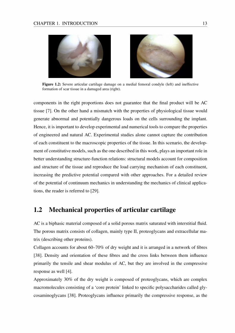
placed by fibrocartilage scar tissue. This is clearly visible in Figure 1.2, which shows two
pictures taken with a fibre-optic camera during an arthroscopy procedure. Cartilage repair
procedures developed by surgeons and scientists in the last decade range from conservative
treatments (e.g. physical therapy or intra-articular injections) to removal of damaged tissue
with open surgery, but ultimately a total joint replacement is usually needed [30] [16]. Bio-
engineering techniques have been proposed to grow tissue engineered AC in vitro and use it
to repair or replace the damaged tissue in vivo.
For this solution to be effective the engineered tissue should replicate AC explants’ me-
chanical properties. However, they are not only the result of the properties of the single
constituents, but also of their organization and mutual interaction. Hence, growing the right
CHAPTER 1. INTRODUCTION 13
Figure 1.2: Severe articular cartilage damage on a medial femoral condyle (left) and ineffectiveformation of scar tissue in a damaged area (right).
components in the right proportions does not guarantee that the final product will be AC
tissue [7]. On the other hand a mismatch with the properties of physiological tissue would
generate abnormal and potentially dangerous loads on the cells surrounding the implant.
Hence, it is important to develop experimental and numerical tools to compare the properties
of engineered and natural AC. Experimental studies alone cannot capture the contribution
of each constituent to the macroscopic properties of the tissue. In this scenario, the develop-
ment of constitutive models, such as the one described in this work, plays an important role in
better understanding structure-function relations: structural models account for composition
and structure of the tissue and reproduce the load carrying mechanism of each constituent,
increasing the predictive potential compared with other approaches. For a detailed review
of the potential of continuum mechanics in understanding the mechanics of clinical applica-
tions, the reader is referred to [29].
1.2 Mechanical properties of articular cartilage
AC is a biphasic material composed of a solid porous matrix saturated with interstitial fluid.
The porous matrix consists of collagen, mainly type II, proteoglycans and extracellular ma-
trix (describing other proteins).
Collagen accounts for about 60–70% of dry weight and it is arranged in a network of fibres
[38]. Density and orientation of these fibres and the cross links between them influence
primarily the tensile and shear modulus of AC, but they are involved in the compressive
response as well [4].
Approximately 30% of the dry weight is composed of proteoglycans, which are complex
macromolecules consisting of a ‘core protein’ linked to specific polysaccharides called gly-
cosaminoglycans [38]. Proteoglycans influence primarily the compressive response, as the
CHAPTER 1. INTRODUCTION 14
glycosaminoglycan links in solution form negatively charged ions that cause the solid matrix
to swell and resist compression.
Interstitial fluid accounts for 70–85% of the total wet weight [38]. The movement of the fluid
through the porous matrix under external compressive loads causes a drag force between the
two phases and consequently significant energy dissipation. This flow-dependent viscoelastic
behaviour is typically negligible in tension [35].
The present work focuses on the mechanical behaviour of the solid phase of the tissue, which
is described in more detail below with focus on the role of the fibre reinforcement. On the
other hand fluid-related phenomena are disregarded.
AC exhibits strong tension-compression asymmetry in experimental tests [54] [34], which is
explained by the selective role of the constituents in the two loading configurations.
In particular, the tensile stiffness is highly strain dependent, and it is determined mainly by
collagen. In the unloaded configuration collagen fibres are wavy. Hence, for small deforma-
tions they realign in the direction of the load rather than stretch, and consequently they do
not bear load. For larger deformations, the external load has to stretch the fibres, generating
higher tensile stress due to the higher stiffness of collagen compared to the soft matrix [66].
This phenomenon, known as fibres engagement, is common for soft biological tissues with
collagen reinforcement [29] and determines a global non-linear response and the presence of
a toe-region in the stress-strain curve.
AC exhibits also a strongly anisotropic and inhomogeneous response under physiological
load, which can be related to the complex organization of the three-dimensional collagen
network. Recent works [37] have shown that the macroscopic response of cartilage cannot
be directly related to the mechanical properties of the individual fibrils at microscale, but that
the tissue strength depends on their arrangement at higher levels. Fibres in immature AC are
mostly oriented parallel to the articular surface throughout the depth, but tissue growth and
remodelling causes the pattern of the fibres to change with age [61] [49]. In mature AC, the
distribution of collagen fibres becomes highly anisotropic and depth-dependent. In particular
three main layers can be identified, which are commonly referred to as superficial, middle
and deep zone [40]. These layers differ in terms of fibres thickness, density and orientation
leading to depth-dependent mechanical properties for the tissue. The superficial zone is the
thinnest one and is characterized by high density of small diameter collagen fibres mostly
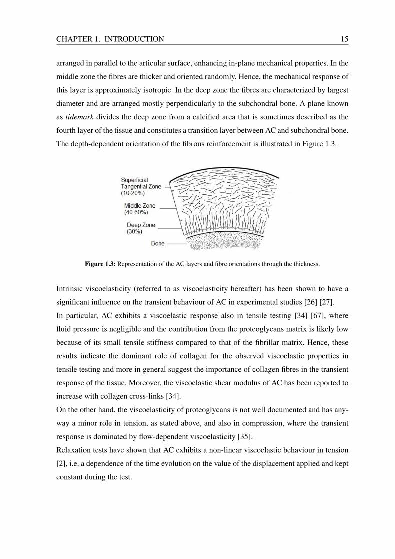
CHAPTER 1. INTRODUCTION 15
arranged in parallel to the articular surface, enhancing in-plane mechanical properties. In the
middle zone the fibres are thicker and oriented randomly. Hence, the mechanical response of
this layer is approximately isotropic. In the deep zone the fibres are characterized by largest
diameter and are arranged mostly perpendicularly to the subchondral bone. A plane known
as tidemark divides the deep zone from a calcified area that is sometimes described as the
fourth layer of the tissue and constitutes a transition layer between AC and subchondral bone.
The depth-dependent orientation of the fibrous reinforcement is illustrated in Figure 1.3.
Figure 1.3: Representation of the AC layers and fibre orientations through the thickness.
Intrinsic viscoelasticity (referred to as viscoelasticity hereafter) has been shown to have a
significant influence on the transient behaviour of AC in experimental studies [26] [27].
In particular, AC exhibits a viscoelastic response also in tensile testing [34] [67], where
fluid pressure is negligible and the contribution from the proteoglycans matrix is likely low
because of its small tensile stiffness compared to that of the fibrillar matrix. Hence, these
results indicate the dominant role of collagen for the observed viscoelastic properties in
tensile testing and more in general suggest the importance of collagen fibres in the transient
response of the tissue. Moreover, the viscoelastic shear modulus of AC has been reported to
increase with collagen cross-links [34].
On the other hand, the viscoelasticity of proteoglycans is not well documented and has any-
way a minor role in tension, as stated above, and also in compression, where the transient
response is dominated by flow-dependent viscoelasticity [35].
Relaxation tests have shown that AC exhibits a non-linear viscoelastic behaviour in tension
[2], i.e. a dependence of the time evolution on the value of the displacement applied and kept
constant during the test.
CHAPTER 1. INTRODUCTION 16
1.3 Constitutive modelling of articular cartilage
A constitutive model of the solid phase of AC should be able to reproduce tension-compression
asymmetry, depth dependent mechanical properties, intrinsic viscoelasticity and finite mul-
tidimensional strains that characterize the response of the tissue to typical load in vivo.
Firstly, these requirements suggest the use of anisotropic finite deformation (i.e. non-linear)
constitutive equations, which are in fact used in most models found in the literature, e.g. [32]
[9] [47]. Another common assumption is that collagen fibres have zero compressive mod-
ulus and carry the load only in tension [34] [32] [9] [47]. Moreover, fibre engagement has
been modelled both implicitly, through a non-linear expression for the potential energy, and
explicitly by mean of an engagement function [1].
The fibre reinforcement in soft biological tissues has often been modelled by means of the so-
called superposition method, in which the potential is the linear combination of an isotropic
term describing the non-fibrous matrix and one or more anisotropic terms associated with
each family of fibres, whose directional information is represented through the definition of
a so-called structure tensor.
While this method is effective for tissues where a finite number of families of fibres can be
identified (e.g. one family for tendon and ligaments [62] and two families for the adventitial
layer of blood vessels [23]), it cannot capture the complexity of the fibre arrangement in AC.
Attempts have been made to adapt this approach by defining a framework of secondary fibre
directions on top of the one defined by the principal fibre directions [31].
A better approach to describe the complex fibre arrangement of AC is to treat the compos-
ite material in statistical terms, i.e. defining a probability distribution density function that
provides at each material point the probability of finding a fibre oriented in a given direction
[33].
Gasser et al. [13] proposed to account for fibres with statistical orientation by calculating
the directional average of the structure tensor. For tissues in which families of fibres can be
identified, it is sufficient to perform only one integration to define a scalar parameter that
accounts for fibre dispersion about the preferred orientation of a specific family. In turn, the
degree of dispersion is used to modulate the level of response, assuming that if the tissue is
stretched in the preferential direction of a family, all the fibres in that family undergo tension
and therefore bear load. This approach was for AC by Pierce [46], who introduced a discrete
CHAPTER 1. INTRODUCTION 17
real fibre distribution extracted from the imaging method described in [36].
An alternative constituent-based approach has been adopted for AC in several works, e.g.
[3] [9] [51]: at each material point the potential associated with the fibres in each direction
is computed and integrated over the unit sphere weighted by a normalized fibre distribution
function. This procedure corresponds to a directional average of the fibre potential. In this
case, the deformation features in the integral, which therefore cannot be calculated a priori.
As a consequence, an analytical use of this potential is impossible.
In particular, Federico and Gasser [9] introduced a three dimensional statistical distribution
function that accounts for both the depth-dependent preferential orientation and the disper-
sion of the fibres. This function was used as an example in this work and is described in detail
in section 3.3. In [9] the numerical evaluation of the integrals is performed using the method
of spherical design, that was adopted for the model presented in the following chapters and
it is discussed in section 3.6.2.
The intrinsic viscoelasticity of collagen fibres has been modelled with linear [57], quasi-
linear [26] and non-linear viscoelastic formulations [43].
One of the first attempts was made by Hayes and Mockros [18], who used a generalized
Kelvin model (a series of Kelvin models). The choice of a linear viscoelastic model is
justified by its simplicity, but it can hardly reproduce the time dependent response of AC.
Moreover, it is only suitable under the assumption of small deformations. The quasi-linear
viscoelastic (QLV) model, originally proposed by Fung [12], is a common choice in the
literature for fibre reinforced tissues [21] [62] and specifically for AC [32]. This approach
preserves the linearity in time but introduces the non-linear relation between stress and strain
typical of highly deformable materials. Hence, it is suitable in the framework of finite defor-
mations. Holzapfel and Gasser [21] developed a time discretisation procedure that eases the
finite element implementation of this model. This method is based on the concept of internal
variables, presented in section 2.5. The derivation for the model developed here is reported
in section 3.6.3. A fully non-linear viscoelastic formulation increases the level of complex-
ity of the model, but it is motivated by experimental evidence of non-linear time dependent
behaviour of the tissue (see section 1.2).
An alternative approach is represented by a constituent-based model in which specific vis-
coelastic parameters are defined for each constituent, as proposed by Vena et al. [62] for lig-
aments. The study showed that a mixture of quasi-linear viscoelastic constituents generates
CHAPTER 1. INTRODUCTION 18
a non-linear response for the whole tissue, as it is discussed in more detail in section 3.2.2,
suggesting a possible explanation for the non-linear viscoelastic behaviour of soft biological
tissues as well as a convenient way to model it. This approach was later adopted to model
the specific case of AC [32].
Recently, Gasser [14] developed an invariant-based framework for finite strain viscoelastic-
ity that describes the viscoelastic continuum as the superposition of a Maxwell body and an
elastic body having two independent reference configurations. This formulation coincides
with the standard quasi-linear models when linearised around the thermodynamic equilib-
rium, but it is valid also for configurations away from it.
1.4 Objective
The long-term goal of the present work was to introduce a hyperelastic constitutive model
for the solid phase of AC that accounts for the anisotropic structural arrangement of the
collagen fibres reinforcement and provides a general approach compatible with a viscoelastic
formulation valid away from the thermodynamic equilibrium (e.g. [14]) and ultimately with
the numerical implementation of the fluid-related response of the tissue.
The primary objective was to introduce an invariant-based viscoelastic formulation of the
free-energy function presented in [9], that represents distributed fibres in a continuum sense
and that accounts for their directional characteristics as well as their intrinsic viscoelastic
behaviour. The specific aims are (1) including the three-dimensional information on the fibre
distribution into a purely structural quantity, i.e. a generalized structure tensor similar to the
one in [13] but suitable for AC, (2) incorporating a viscoelastic formulation valid around
the thermodynamic equilibrium and capable of reproducing the non-linear time-dependent
behaviour of the tissue in tension, (3) deriving the corresponding numerical model and im-
plementing an efficient solution procedure.
Chapter 2
Continuum mechanical framework
In this chapter an overview of the main aspects of continuum mechanics at large defor-
mations is provided, as it represents the theoretical foundation of the model developed in
this work. Starting from the definition of basic quantities like strains and stresses, the focus
moves towards the specific case of biological tissues through the concepts of hyperelasticity,
incompressibility and fibre reinforcement, concluding with viscoelasticity at large deforma-
tions. Finally the concept of elasticity tensor is introduced, which is fundamental for the
numerical implementation of the model.
2.1 Motion and deformation gradient
A deformable body, within the framework of 3D Euclidean space R3, can be described as a set
of interacting particles embedded in the domain Ω ∈ R3. Among all possible configurations
assumed by the body during its motion, one is chosen as reference and denoted as Ω0. In this
configuration, every point in the body is uniquely identified by the position vector
X = XIEI I = 1, . . . , 3 (2.1)
where E1,E2,E3 is the basis of the underlying coordinate system. For simplicity, the
orthogonal cartesian basis is used. The motion of the body to the so-called current configu-
ration Ωϕ can be described as the combination of the motion of all its points
x = xiei i = 1, . . . , 3 (2.2)
19
CHAPTER 2. CONTINUUM MECHANICAL FRAMEWORK 20
where e1, e2, e3 is the basis of the current configuration. In this work it assumed that the
two sets of base vectors are coincident, i.e. EI ≡ ei, which is convenient since all the possible
motions take place within the Euclidean space.
In the following, capital letters are used to identify entities related to the reference (also
called material or Lagrange) configuration, and small letters for those related to the current
(also called spatial or Eulerian) reference.
The simplification used in the linear theory that the two sets of coordinates XI and xi are
also coincident cannot be used in the context of finite elasticity due to the large displace-
ments involved.
To describe the deformation process locally, a tensor F is introduced which maps a material
line element of the initial configuration dX in the reference configuration, to a line element
dx in the current configuration.
dx = FdX or dxi = FiJdXJ (2.3)
In the equation above F represents a gradient and it is therefore known as deformation gra-
dient. Thus, the components of F are given by the partial derivatives xi,J = ∂xi/∂XJ :
F =∂xi∂XJ
ei ⊗ EJ or FiJ =∂xi∂XJ
(2.4)
The inverse of the deformation gradient F−1 defines the inverse relation
dX = F−1dx (2.5)
It is now possible to express the transformation of differential surface elements, which is
given by Nanson’s formula (see e.g. [25])
da = nda = JF−TNdA = JF−TdA (2.6)
where J = detF and N and n are the normal vectors corresponding to dA and da, respec-
tively.
The transformation between volume elements, defined as the scalar product of infinitesimal
CHAPTER 2. CONTINUUM MECHANICAL FRAMEWORK 21
surface element and an infinitesimal vector, is immediately given by
dv := dx · dan = FdX · JF−TdAn = JdV (2.7)
which shows that J represent a volume ratio. To exclude self-penetration of the body and
ensure that the deformation gradient is non singular (i.e. invertible), F should then fulfil the
following condition:
J = detF > 0 (2.8)
The deformation gradient F represents the transformation of dX into dx and it includes
the changes in modulus, direction and orientation. However, the deformation is related only
to the change in length of an infinitesimal vector. Hence, the motion can be split into the
sequence of a deformation and a rotation through a polar decomposition:
F = RU with RT = R−1 ; UT = U (2.9)
where the orthogonal tensor R is an isometric transformation that changes only direction and
orientation of a vector and the positive definite symmetric tensor U, defined by the relation
‖dx‖ = ‖UdX‖, is known as the right stretch tensor.
2.2 Strain measures
Unlike displacements, strains are not measurable quantities. They are introduced to simplify
analyses and are based on a concept, allowing many possible definitions. Those presented
in this section represent the most common choices in solid mechanics and are based on the
definition of rotation-independent deformation tensors.
The distance between two sufficiently close points X and Y in the reference configuration
can be expressed as
dX = dεm0 with dε = |Y −X| , m0 =Y −X
|Y −X|(2.10)
where dε is a scalar value and m0 is a unit vector (i.e. |m0| = 1).
The deformation gradient F can then be used to compute the corresponding vector dx in
the spatial configuration. In particular the application of F to the unit vector m0 provides a
CHAPTER 2. CONTINUUM MECHANICAL FRAMEWORK 22
measure of the stretch applied in the direction of m0
λm0(X) = F(X)m0 (2.11)
The vector λm0 is the so-called stretch vector and its modulus λ is known as stretch ratio.
The stretch ratio can be used to determine whether during the deformation a line element
was compressed (λ < 1), unstretched (λ = 1) or extended (λ > 1).
It is then possible to define the right Cauchy-Green deformation tensor C through the square
of the stretch ratio:
λ2 = λm0 · λm0 = Fa · Fa = m0 · FTFa = m0 ·Ca (2.12)
C = FTF or CIJ = FiIFiJ (2.13)
Using the properties of U and R, C can be written as
C = FTF = UTRTRU = UTU = U2 (2.14)
which confirms that C is purely a measure of the deformation.
Also, the right Cauchy-Green tensor is symmetric and positive definite ∀x ∈ Ω:
C = FTF = (FTF)T = CT and u ·Cu > 0 ∀u 6= 0 (2.15)
At this point a strain measure can be introduced to evaluate how much a given displace-
ment differs locally from a rigid body displacement. The Green-Lagrange strain tensor E is
derived from the change in the squared lengths:
1
2
[(λdε)2 − dε2
]=
1
2
[(dεm0) · FTF (dεm0)− dε2
]= dX · EdX (2.16)
E =1
2
(FTF− I
)=
1
2(C− I) or EIJ =
1
2(FiIFiJ − δIJ) (2.17)
The Green-Lagrangian strain tensor is a measure of how much C differs from I and therefore
it equals zero when no deformation is acting on the body. Also, given the symmetry of C and
I, E is obviously symmetric.
It should be noted that the tensors C and E operate solely in material reference. Similarly,
a deformation measure can be derived with respect to the spatial configuration. For this
CHAPTER 2. CONTINUUM MECHANICAL FRAMEWORK 23
purpose the inverse stretch vector λ−1mϕ in the direction of mϕ, for each x ∈ Ωϕ might be
define as:
λ−1mϕ(x) = F−1(x)mϕ (2.18)
In analogy with the definitions for the reference configuration, the norm λ−1 of the inverse
stretch vector λ−1mϕ is known as inverse stretch ratio and the unit vector mϕ identifies the
direction of the spatial line element dx, with dx = dεmϕ.
The left Cauchy-Green tensor is defined trough the square of the inverse stretch ratio:
λ−2 = λ−1mϕ · λ−1
mϕ = F−1mϕ · F−1mϕ = mϕ · F−TF−1mϕ = mϕ · b−1mϕ (2.19)
where b is the left Cauchy-Green tensor, given by
b = FFT or bij = FiIFjI (2.20)
As the corresponding tensor in material description, b is symmetric and positive definite
∀xϕ ∈ Ωϕ:
b = FFT = (FTF)T = bT and u · bu > 0 ∀u 6= 0 (2.21)
The most used strain measure in the spatial configuration is the Euler-Almansi tensor e,
which is defined using the change in square length similarly to the Green-Lagrange tensor in
material reference (in fact e is the push-forward of the E). In particular, with the use of 2.19,
the expression of the strain tensor is given by
1
2
[dε2 − (λ−1dε)2
]=
1
2
[dε2 − (dεmϕ) · F−TF−1(dεmϕ)
]= dx · edx (2.22)
e =1
2
(I− F−TF−1
)=
1
2
(I− b−1
)or eij =
1
2
(δIJ − F−1
Ii F−1Ij
)(2.23)
2.3 Stress measures
In continuum mechanics, stress is a physical quantity that expresses the internal forces that
neighbouring particles of a continuous material exert on each other. Quantitatively, the stress
is expressed by the traction vector, defined as the traction force F between adjacent parts of
the material across an imaginary separating surface, divided by the area of the surface. The
CHAPTER 2. CONTINUUM MECHANICAL FRAMEWORK 24
infinitesimal force acting on a surface element df can be defined as
df = tda = TdA (2.24)
where t is defined with respect to the spatial configuration and it is known in the literature
as the Cauchy traction vector, while the (pseudo) traction vector T is defined with respect to
the material configuration and it is known as first Piola-Kirchhoff traction vector.
The well-known Cauchy stress theorem postulates the existence of tensor fields σ and P such
that:
t(x,n) = σ(x)n or ti = σijnj (2.25)
T(X,N) = P(X)N or Ti = PiINI (2.26)
where N and n are the normals corresponding to the surface elements dA and da, while
the tensor σ denotes the symmetric Cauchy (or true) stress tensor and P denotes the first
Piola-Kirchhoff (or nominal) stress tensor.
The stress tensors are related by the so-called Piola transformation, given by the substitution
of (2.25) and (2.26) into (2.24) and the use of the Nanson’s formula:
P = JσF−T or PiI = JσijF−1Ij (2.27)
Another stress tensor acting on the spatial configuration and often used in computational
mechanics is known as Kirchhoff stress tensor τ and it is defined as
τ = Jσ or τij = Jσij (2.28)
It should be noted that the first Piola-Kirchhoff stress tensor is in general non-symmetric,
which complicates its use in computational mechanics. To overcome this problem, the so-
called second Piola-Kirchhoff stress tensor S has been introduced, computed by performing
the pull-back operation on the spatial tensor τ :
S = F−1τF−T or SIJ = F−1Ii F
−1Jj τij (2.29)
The stress tensor S does not have any physical interpretation in terms of surface tractions.
Nevertheless, it is very useful in computational mechanics because it is symmetric and in
CHAPTER 2. CONTINUUM MECHANICAL FRAMEWORK 25
the definition of constitutive relation because it acts on the material reference and it is work
conjugate to the Green-Lagrange strain tensor.
Finally, the second Piola-Kirchhoff stress tensor can be related to the Cauchy stress substi-
tuting (2.28) into 2.29:
S = JF−1σF−T = F−1P = ST or SIJ = JF−1Ii F
−1Jj σij = F−1
Ii PiJ = SJI (2.30)
where the use of (2.27) reveals also the relation with the first Piola-Kirchhoff stress tensor
P = FS or PiI = FiJSJI (2.31)
2.4 Hyperelastic materials
A so-called hyperelastic material postulate the existence of a Helmotz free-energy function
Ψ, which is defined per unit reference volume rather than per unit mass. If Ψ is only function
of some strain tensor, the Helmotz free-energy function is referred to as the strain-energy
function and both the terminologies will be use in this work.
A hyperelastic material is defined as a subclass of an elastic material whose response can be
expressed as
P =∂Ψ(F)
∂For σ = J−1∂Ψ(F)
∂FFT (2.32)
with respect to the material or the spatial configuration respectively.
It is assumed throughout this work that the strain-energy function vanishes in the reference
configuration, i.e. when F = I. Also, the strain-energy function should increase with the de-
formation to guarantee physical behaviour. Thus, the range of admissible functions is limited
by the following two conditions:
Ψ = Ψ(I) = 0; Ψ = Ψ(F) ≥ 0 (2.33)
It follows that the residual stress (i.e. the stress in the undeformed configuration) is assumed
to be zero. The reference configuration is therefore defined as stress-free. The strain energy
function should also be objective, i.e. translations and rotations should not affect the amount
of energy stored in the body. This is represented by the restriction
Ψ(F) = Ψ(QF) (2.34)
CHAPTER 2. CONTINUUM MECHANICAL FRAMEWORK 26
where Q is an orthogonal tensor. Hence, using the polar decomposition (2.9) and choosing
the transpose of the proper orthogonal rotation tensor as a specific case for Q, it is possible
to write
Ψ(F) = Ψ(RTF) = Ψ(RTRU) = Ψ(U) (2.35)
Using (2.14) and (2.32) it is finally possible to write the potential energy and the stress tensor
as a function of C:
Ψ(F) = Ψ(C) ⇒ P =∂Ψ(C)
∂C
∂C
∂F= 2F
∂Ψ(C)
∂C(2.36)
2.4.1 Incompressible hyperelastic materials
Materials that keep the volume constant throughout a motion are characterized by the incom-
pressibility constraint, that can be expressed as
J = detF = 1 or J2 = detC = 1 (2.37)
It is possible to separate the volumetric part and the isochoric part of the free-energy function,
which is convenient when incompressible materials are studied because they show strong
differences between the bulk and the shear behaviour.
To do this, the deformation gradient F is decomposed into
F = (J1/3I)F (2.38)
where (J1/3I) represents the dilatation part and F the distorsional part, so that detF = 1.
The tensor F can be defined as isochoric deformation gradient. Consequently the modified
right and left Cauchy-Green tensors can be defined as
C = FTF = J2/3C, C = FTF (2.39)
b = FFT = J2/3b, b = FFT (2.40)
The free-energy function can then be written as
Ψ(C) = U(J) + Ψ(C) (2.41)
where U(J) and Ψ(C) describe the volumetric and the isochoric contribution to the poten-
CHAPTER 2. CONTINUUM MECHANICAL FRAMEWORK 27
tial, respectively. If a much higher external work is required to generate dilatational than
distorsional changes the material is defined nearly-incompressible. For this class of material
(that include biological tissues) the compressibility effects are small and it is still possible
to use the decoupled form of the potential. It should also be noted that for incompressible
materials it is not necessary to define U(J).
Accordingly, the second Piola-Kirchhoff stress tensor can be computed by mean of the addi-
tive split
S = 2∂Ψ(C)
∂C= 2
∂[U(J) + Ψ(C)]
∂C= Svol + S (2.42)
It is necessary to compute the derivative of the modified right Cauchy-Green tensor C relative
to C. Given the definition of J2 in (2.37), the introduction of the standard expression for the
derivative of the determinant of a second order tensor leads to
∂J2
∂C=∂(det(C))
∂C= det(C)[C−1]T = J2C−1 (2.43)
which gives
∂J2
∂C= 2J
∂J
∂C=⇒ ∂J
∂C=J
2C−1 (2.44)
∂J−2/3
∂C= −2
3J−2/3 ∂J
∂C= −1
3J−2/3C−1 (2.45)
Hence, the derivative of C relative to C is given by
∂C
∂C=∂[J−2/3C]
∂C= J−2/3∂C
∂C+ C⊗ ∂J−2/3
∂c= J−2/3
[I− 1
3(C⊗C−1)
]︸ ︷︷ ︸
PT
= J−2/3PT
(2.46)
where I is the fourth order identity tensor, defined as A = I : A (where A is a second order
tensor) and PT defines the projector tensor (with respect to the reference configuration)
P = I− 13(C−1⊗C), which furnishes the deviatoric operator so that [P : (·)] : C = dev(·) :
C = 0.
It is then possible to compute
Svol = 2∂U(J)
∂J
∂J
∂C= pJC−1 (2.47)
CHAPTER 2. CONTINUUM MECHANICAL FRAMEWORK 28
S = 2∂Ψ(C)
∂C
∂C
∂C= J−2/3P : S = J−2/3devS (2.48)
where p = ∂U(J)/∂J is the hydrostatic pressure and S = 2∂Ψ/∂C is a (fictitious) iso-
choric second Piola-Kirchhoff stress. Under the hypothesis of incompressibility the hydro-
static pressure is a Lagrange multiplier and can only be determined from the boundary con-
ditions.
The Cauchy stress can be compute through an inverse Piola transformation of (2.42)
σ = J−1χ∗[S] = σvol + σ or σij = J−1FiIFjJSIJ (2.49)
with
σvol = pχ∗[C−1] = pI (2.50)
σ = J−5/3χ∗[P] : χ∗[S] = J−2/3p : σ (2.51)
where p = I− 13(I⊗ I) furnishes the deviatoric operator in the spatial configuration, so that
[p : (·)] : I = 0 and σ = J−1χ∗[S] is the (fictitious) isochoric Cauchy stress.
2.4.2 Isotropic hyperelastic materials
A material is considered isotropic if its response in a stress-strain test is the same in all direc-
tion. In other words, a hyperelastic material is isotropic relative to the reference configuration
Ω0 if a motion superimposed on any particularly translated and/or rotated leads to the same
strain-energy function. This condition is guaranteed by the following equality
Ψ(F) = Ψ(FQT) (2.52)
where F is the deformation gradient and Q is an orthogonal tensor, which in turn can be
expressed as a function of the right Cauchy-Green tensor C as
Ψ(C) = Ψ(QFTFQT) = Ψ(QCQT) (2.53)
CHAPTER 2. CONTINUUM MECHANICAL FRAMEWORK 29
According to the representation theorem for invariants, every strain energy function that
possesses this property can be expressed as a set of independent invariants of its argument,
Ψ(C) = Ψ(I1(C), I2(C), I3(C)) (2.54)
where Ia(C), a = 1, 2, 3 are the standard invariants of the right Cauchy-Green tensor
I1 = tr(C), I2 =1
2
[(tr(C))2 − tr(C2)
], I3 = det(C) (2.55)
Introducing the decoupled form of the potential and the incompressibility assumption (i.e.
I3 = J2 = 1, see (2.37)), the isochoric part of the strain-energy can be written as a function
of the first and the second invariant of the modified right Cauchy-Green tensor
Ψ(C) = Ψ(I1(C), I2(C)) (2.56)
The so called neo-Hookean model is the simplest representation of this class of materials
and it extends the Hooke’s law for linear materials to the range of large deformation. The
expression of the isochoric strain-energy function reads
Ψ(C) = c1(I1 − 3) (2.57)
where c1 is a material parameter equal to half of the shear modulus in the reference configu-
ration and I1 = tr(C) is the first invariant of the modified right Cauchy-Green tensor.
2.4.3 Fibre reinforced hyperelastic materials
Biological tissues are usually composed of a matrix material and one or more families of
fibres that generate strong directional properties and anisotropic mechanical behaviour. It is
assumed that the fibres have single preferred direction, that they are continuously distributed
throughout the material and that they are the only source of anisotropy. Moreover, micro-
mechanical aspects are disregarded.
A material reinforced by one family of fibres typically shows much higher stiffness in the
fibre direction and is isotropic in all the directions orthogonal to the fibres. This symmetry
properties is called transverse isotropy. For this class of materials, the stress at a material
CHAPTER 2. CONTINUUM MECHANICAL FRAMEWORK 30
point depends on the deformation gradient, but also on the direction of the fibres throughout
the material, which can be described in the reference configuration by a unit vector field
a0(X), |a0| = 1. After the deformation, the fibres will have a new preferred direction, de-
fined by a unit vector field a(x), |a| = 1, but also a new length. Hence, the stretch λ defined
in (2.11), that is related to the right Cauchy-Green tensor by (2.13), must also be determined.
The fibre direction in the reference configuration must be included in the expression of the
free energy. In particular, since the sense of a0 is immaterial, the potential is chosen as an
even function of a0 and the second order tensor H, known as structure tensor, is introduced
as an argument:
H = a0 ⊗ a0, Ψ = Ψ(C, a0 ⊗ a0) (2.58)
It should be noted that objectivity is trivially satisfied as the potential is function of quantities
defined with respect to the reference configuration.
It can be shown (e.g. see [25]) that the requirement for transverse isotropy becomes
Ψ(C, a0 ⊗ a0) = Ψ(QCQT,Qa0 ⊗ a0QT) (2.59)
Similarly to the case of isotropy, it is also possible to write the potential using a set of
independent invariants, but it is necessary to define two additional invariants in order to fulfil
(2.59) (a complete description is given in [56]):
I4(C, a0) = a0 ·Ca0 = λ2 , I5(C, a0) = a0 ·C2a0 (2.60)
The invariants above describe the properties of the fibres and their interaction with other ma-
terial constituents.
The same approach can be extended to materials with more than one family of fibres by intro-
ducing similar invariants for each family and additional expression describing the anisotropy
generated by the interaction of different families.
2.5 Viscoelasticity at finite deformation
In this section a three-dimensional viscoelasticity framework based on the concept of inter-
nal variables is described, that is suitable for highly deformable materials. This approach is
CHAPTER 2. CONTINUUM MECHANICAL FRAMEWORK 31
convenient for the definition of numerical models using the finite element method and it can
be applied to highly deformable materials for small perturbation away from the equilibrium
state. For these reasons it is commonly used in the literature, e.g. see [52] [20].
Internal variables describe aspects of the internal structure of materials associated with dis-
sipative effects, and they are introduced as phenomenological variables constructed math-
ematically within a macroscopic framework (similarly to the ‘dashpot elements’ in linear
viscoelastic models). They influence strain and stresses, and they are often referred to as his-
tory variables (Γα) since their evolution reflects the history of the deformation. The current
state of a viscoelastic material can then be described by the deformation gradient and the
current values of a set of internal variables (note that strain is independent of past values of
history variables).
In accordance with the previous sections a decoupled representation of the strain-energy
function is used. The change of the potential from the reference to the current configuration
within a isothermal transformation is then given by
Ψ(C,Γ1, . . . ,Γm) = U∞(J) + Ψ∞(C) +m∑α=1
Υα(C,Γα) (2.61)
The first two terms, U∞(J) and Ψ∞, describe the equilibrium state of the solid. According to
(2.41), they represent the volumetric and the isochoric part of the elastic response as t→∞,
respectively. The additional term represents the ‘dissipative’ viscoelastic contribution.
A common assumption, based on experimental evidence, is that the time-dependent prop-
erties are function only of the isochoric part of the deformation. Thus, the volumetric part
remains fully elastic and can be described with the equation introduced in section 2.4.1. The
viscoelastic behaviour instead is function of the modified right Cauchy-Green tensor C and
it is modelled as the superposition of α = 1, . . . ,m viscoelastic processes, each character-
ized by a particular relaxation time τα ∈ (0,∞), which characterizes the rate of decay of
stress and strain. The condition of non-negative internal dissipation, required by the second
law of thermodynamics, can be enforced using the Coleman-Noll procedure (for a complete
description the reader is referred to [25]), which leads to the following expressions for the
CHAPTER 2. CONTINUUM MECHANICAL FRAMEWORK 32
Second Piola-Kirchhoff stress tensor and the internal dissipation:
S = 2∂Ψ(C,Γ1, . . . ,Γm)
∂C= S∞vol + S∞ +
m∑α=1
SVα (2.62)
Dint = −m∑α=1
2∂Υα(C,Γα)
∂Γα
:1
2Γα ≥ 0 (2.63)
where the tensor variables SVα have been introduced, which represent non-equilibrium stresses.
This quantity is defined in analogy with (2.48)
SVα = J−2/3P : SVα with SVα = 2∂Υα(C,Γα)
∂C(2.64)
where the fictitious non-equilibrium stress SVα is introduced. Based on the equilibrium equa-
tion for a linear viscoelastic solid, the non-equilibrium stresses can be related to the strain-
like quantities Γα resulting in an equivalent expression for the internal dissipation:
SVα = −2∂Υα(C,Γα)
∂Γα
⇒ Dint =m∑α=1
SVα :Γα
2≥ 0 (2.65)
Additional equations of evolution must be defined in order to satisfy the inequality (2.63)
(i.e. the condition of local entropy production). An extension of the evolution equations for
the linear case leads to˙SV
α +SVατα
= ˙Sα , α = 1, . . . ,m (2.66)
which is valid for a semi-open time interval t ∈ (0, T ]. The values of the internal variables
at initial time t = 0 are assumed to be zero, since a stress-free reference configuration is
considered. The tensor Sα is the isochoric second Piola-Kirchhoff stress corresponding to the
system related to the α-relaxation process with relaxation time τα ∈ (0,∞). Sα is defined
according to equation (2.48) as
Sα = J−2/3P : Sα (2.67)
where Sα = 2∂Ψα/∂C is a (fictitious) isochoric second Piola-Kirchhoff stress.
The set of linear equations (2.66) has a physical basis, provides a good approximation of
the behaviour of real materials under large deformation and it is also suitable for efficient
numerical time integration scheme.
Finally, disregarding an instantaneous response at t = 0 the closed form solution of equations
CHAPTER 2. CONTINUUM MECHANICAL FRAMEWORK 33
(2.66) is given by the convolution integrals
SVα =
∫ t=T
t=0
exp
−(T − t)
τα
˙Sα(t) dt (2.68)
The integral (2.68) defines a so-called quasi-linear viscoelastic response: compared to a
standard linear viscoelastic model, the relation between stress and strain becomes non-linear
due to finite deformations but the linearity in the time domain is preserved.
2.6 Elasticity tensor
In order to compute the solution of non-linear problems in finite elasticity, a sequence of
linearised problem is derived using Newton-like techniques, and solved instead. Hence, from
the computational point of view it is important to derive a linearisation of the constitutive
relations defined above.
The non-linear second Piola-Kirchhoff stress tensor S is assumed to be solely a tensor-valued
function of one tensorial variable, in particular the right Cauchy-Green tensor C. A first order
Taylor expansion of S around C then gives
S(C + dC) = S(C) + dS +O(dC) (2.69)
with
dS =∂S(C)
∂C: dC = 2
∂S(C)
∂C:
1
2dC (2.70)
where
C = 2∂S(C)
∂Cor CIJKL = 2
∂SIJ∂CKL
(2.71)
is known as elasticity tensor and represent the derivative of S relative to C and it is therefore
a fourth order tensor. The elasticity tensor relates the work conjugate pairs of stress and strain
tensors, measuring the change of stress resulting from a change in strain.
It should be emphasized that for hyperelastic materials C possesses minor and major sym-
metries. The minor symmetries can be expressed in index form as
CIJKL = CJIKL = CIJLK (2.72)
and they arise from the symmetries of S and C. Therefore they are typical of all elastic
CHAPTER 2. CONTINUUM MECHANICAL FRAMEWORK 34
materials and they do not require the existence of a hyperelastic potential.
On the other hand, the major symmetries hold if a hyperelastic strain-energy functionΨ is de-
fined. Using the definition of the second Piola-Kirchhoff with respect to the potential energy
(2.42) it is possible to write
C = 2∂
∂C
[2∂Ψ(C)
∂C
]= 4
∂2Ψ(C)
∂C∂Cor CIJKL = 4
∂2Ψ
∂CIJ∂CKL(2.73)
which directly provides the symmetry relation
C = CT or CIJKL = CKLIJ (2.74)
Due to the symmetries, the elasticity tensor C has only 21 independent components. The ma-
jor symmetries are particularly important from a numerical point of view as they guarantee
the symmetry of the tangent stiffness matrix in a finite element formulation.
The elasticity tensor in spatial reference is computed through an inverse Piola transformation
(sometimes in the literature a normal push-forward operation is used instead):
c = J−1χ∗[C] or cijkl = J−1FiIFjJFkKFlLCIJKL (2.75)
Minor and major symmetries hold also in the spatial reference (the latter only if hyperelastic
potential can be defined).
According to the decoupled definition of the second Piola-Kirchhoff stress tensor (2.42) the
elasticity tensor in material reference can be written as
C = 2∂Svol(C)
∂C+ 2
∂S(C)
∂C= Cvol + C (2.76)
Using arguments introduced in previous sections, a straightforward but lengthy calculation
that for brevity is not reported here (see e.g. [25]) leads to the following expression for
volumetric and isochoric contribution:
Cvol = JpC−1 ⊗C−1 − 2JpIC−1 (2.77)
C = J−4/3P : C : P +2
3Tr(J−2/3S)P− 2
3(C−1 ⊗ S + S⊗C
−1) (2.78)
CHAPTER 2. CONTINUUM MECHANICAL FRAMEWORK 35
where the scalar function p = p + J(dp/dJ), the referential isochoric (fictitious) elasticity
tensor C = 4∂2Ψ/∂C2 and the fourth order tensor [IC−1 ]IJKL = 12(C−1
IKC−1JL + C−1
ILC−1JK) are
introduced. Moreover, the referential trace operator Tr[·] := [·] : C and the referential fourth
order projection tensor P = IC−1 − 13(C−1 ⊗C−1) are utilized.
An inverse Piola transformation of (2.76) gives the definition of the decoupled elasticity
tensor in the spatial configuration
c = J−1χ∗[C] = cvol + c (2.79)
with
Cvol = pI⊗ I− 2pI (2.80)
C = J−4/3p : c : p +2
3J−2/3tr(σ)p− 2
3[I⊗ σ + σ ⊗ I] (2.81)
where c = J−1χ∗[C] is the spatial isochoric (fictitious) elasticity tensor and the spatial trace
operator tr[·] := [·] : I is utilized.
The equations above are compact notations for the material and spatial tensors, but an effi-
cient finite element implementation requires these expressions to be elaborated for a partic-
ular constitutive model.
Chapter 3
Methods
In this chapter the constitutive equations and the relative numerical implementation are de-
scribed. It is assumed that fibres are continuously distributed throughout the material so that
the continuum theory of fibre reinforced composite materials (see section 2.4.3, or [25] for a
complete discussion) is the constitutive theory of choice. The elastic strain energy function
of a material with statistical fibre distribution is obtained from that of a composite material
with a family of perfectly aligned fibres by using a directional average of the structure tensor
(2.58) and suitably modified to account for tension compression asymmetry of collagen fi-
bres. The stress and elasticity tensors are computed as the first and second derivatives of the
elastic potential with respect to a suitable strain measure. A probability distribution function
is also proposed and its use in the model is discussed. Finally, the main aspects of the finite
element implementation are outlined and some illustrative examples are described.
3.1 Structure tensor
Soft tissues with fibre reinforcement are often modelled using the superposition method and
including the directional information of each family of fibres into a structure tensor (see sec-
tion 2.4.3). However, the complex three-dimensional network of collagen that characterizes
AC can be more effectively modelled as one family of fibres statistically distributed around
a polar axis.
To account for such configuration, it was proposed in [13] to define a generalized structure
tensor by calculating the directional average of the structure tensor (2.58). For completeness
and continuity, the derivation of this tensor is reported below, as it represents the foundation
of the one introduced in section 3.2 for the specific case of AC.
36
CHAPTER 3. METHODS 37
Following [13], an orthonormal basis of the Eulerian space R3 is considered. The choice of
the basis is arbitrary, but for sake of simplicity the canonical basis (e1, e3, e3) is used. A
generic unit vector M (|M| = 1) can be expressed in polar coordinates as function of the co-
latitude Θ from the polar axis K (without loss of generality K = e3 is chosen) and longitude
Φ from the e1 − e3 plane as
M(Θ,Φ) = sin Θ cos Φ e1 + sin Θ sin Φ e2 + cos Θ e3. (3.1)
where Θ ∈ [0, π] and Φ ∈ [0, 2π] (see Figure 3.1). For each M,−M is also included in the
ranges of the Eulerian angles.
A probability distribution ρ(M) is introduced, that characterizes the distribution of fibres in
the reference configuration Ω0. The distribution is defined such that ρ(M(Θ,Φ)) sin ΘdΘdΦ
represents the number of fibres with orientation in the range [(Θ,Θ +dΘ), (Φ,Φ +dΦ)] (see
Figure 3.1). Moreover, it has to obey the symmetry condition ρ(M) ≡ ρ(−M) and to be
normalized over the unit sphere such that
1
4π
∫S2
ρ(M(Θ,Φ)) dS =1
4π
∫ 2π
0
∫ π
0
ρ(Θ,Φ) sin Θ dΘ dΦ = 1 (3.2)
where S2 is the unit sphere and the polar representation of M was used to express the proba-
bility distribution as a function of Θ and Φ.
The directional average of any function f(M) is then given by
〈f〉 =1
4π
∫S2
ρ(M)f(M) dS =1
4π
∫ 2π
0
∫ π
0
ρ(Θ,Φ)f(M(Θ,Φ)) sin Θ dΘ dΦ (3.3)
Due to the symmetry requirement on the density function, only general orthotropic distri-
butions are suitable to represent the fibres. In particular, a transversely isotropic distribution
around the polar axis K = e3 is chosen, that is sufficient to describe the fibre arrangement
characterizing the three zones of AC (see section 1.2). Hence, the distribution is independent
of the longitude Φ and the normalization condition becomes∫ π
0
ρ(Θ) sin Θ dΘ = 2 (3.4)
Following [13], a (symmetric) generalized structure tensor of second order can then be in-
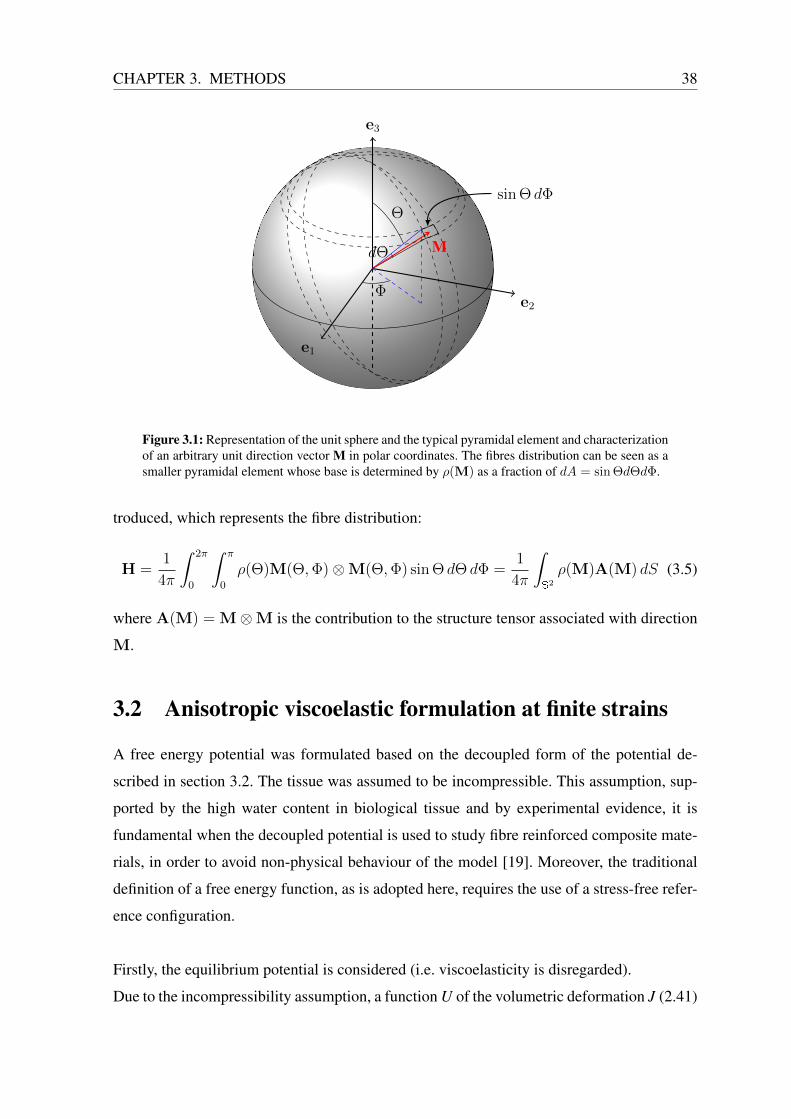
CHAPTER 3. METHODS 38
e1
e2
e3
Φ
Θ
dΘ M
sin Θ dΦ
Figure 3.1: Representation of the unit sphere and the typical pyramidal element and characterizationof an arbitrary unit direction vector M in polar coordinates. The fibres distribution can be seen as asmaller pyramidal element whose base is determined by ρ(M) as a fraction of dA = sin ΘdΘdΦ.
troduced, which represents the fibre distribution:
H =1
4π
∫ 2π
0
∫ π
0
ρ(Θ)M(Θ,Φ)⊗M(Θ,Φ) sin Θ dΘ dΦ =1
4π
∫S2
ρ(M)A(M) dS (3.5)
where A(M) = M⊗M is the contribution to the structure tensor associated with direction
M.
3.2 Anisotropic viscoelastic formulation at finite strains
A free energy potential was formulated based on the decoupled form of the potential de-
scribed in section 3.2. The tissue was assumed to be incompressible. This assumption, sup-
ported by the high water content in biological tissue and by experimental evidence, it is
fundamental when the decoupled potential is used to study fibre reinforced composite mate-
rials, in order to avoid non-physical behaviour of the model [19]. Moreover, the traditional
definition of a free energy function, as is adopted here, requires the use of a stress-free refer-
ence configuration.
Firstly, the equilibrium potential is considered (i.e. viscoelasticity is disregarded).
Due to the incompressibility assumption, a function U of the volumetric deformation J (2.41)
CHAPTER 3. METHODS 39
does not need to be defined. Moreover, it is assumed that the isochoric part of the free energy
function can be expressed as the superposition of an isotropic potential Ψ∞g related to the
ground matrix and and a potential Ψ∞f due to the collagen fibre distribution
Ψ∞(C,H) = φgΨ∞g (C) + φf Ψ
∞f (C,H) (3.6)
where H is defined in accordance with (3.5) and depends on a concentration parameter and
the Cauchy-Green tensor, as will be explained in more details below.
Several works, e.g. [24] [13] [1], model the ground matrix as an incompressible isotropic
neo-Hookean material. Due to the complexity of the composition of AC (see section 1.2),
this might be a too restrictive simplification. Nevertheless, in view of its simplicity, this
assumption is adopted here. Hence the free energy function associated with the matrix reads
Ψ∞g (C) =1
2c0(I1 − 3) (3.7)
where c0 denotes the neo-Hookean parameter (i.e. the shear modulus of the matrix) and I1 is
the standard definition of the first invariant of C
I1 = C : I = tr(C) (3.8)
The fibre contribution is split into an isotropic contribution, that accounts for the different
‘passive’ mechanical properties with respect to the ground matrix, and an anisotropic contri-
bution that accounts for the transversely isotropic properties of the fibres.
Ψ∞f (C,H) = Ψ∞fi (C) + Ψ∞fa(C,H) (3.9)
For simplicity, the isotropic contribution is modelled as a neo-Hookean material character-
ized by a parameter cfi 6= c0 , i.e.
Ψ∞fi (C) =1
2cfi(I1 − 3) (3.10)
As described in section 1.2, collagen fibres are wavy in the reference configuration and the
load required to straighten them can be neglected when compared to the load that they trans-
mit once stretched (i.e. collagen fibres are assumed to transmit load only if stretched beyond
the point where undulations disappear). This phenomenon can be effectively modelled by
CHAPTER 3. METHODS 40
means of a non-linear expression for the potential and such solution was adopted in this work.
It is reported in the literature that a quadratic function may be sufficient to effectively repro-
duce the behaviour of AC in different cases of interest, e.g. immature or engineered cartilage,
that do not exhibit strong non-linearity at large deformations [51]. Hence, the second-order
polynomial form
Ψ∞fa(C,H) =1
2cfaE
2 =1
2cfa(I4 − 1)2 (3.11)
is proposed to particularize the fibre contribution, where cfa > 0 is a stress-like parameter to
be determined from mechanical tests of the tissue and I4 denotes an invariant of the symmet-
ric generalized structure tensor (see [56] for a general discussion of invariants of this kind),
defined as
I4 = H : C (3.12)
The same invariant can be defined for each component of the structure tensor, i.e
IM4 = A : C = (M⊗M) : C = M · CM = λ2M (3.13)
where it is clearly shown that the distorsional invariant IM4 represents the squared stretch
in the direction M, i.e. the distortional fibre stretch under the hypothesis of perfect bonding
between fibres and matrix. Note that A : I = H : I = 1. I4 can be interpreted as an extension
of (3.13) and it is used to define the Green-Lagrange strain-like quantity E = H : C − 1,
which characterizes the weighted averaged strain of the fibres at the material point.
Finally, it is assumed that collagen fibres would buckle under the smallest compressive load
(i.e. they are characterized by zero compressive modulus) [34]. This modelling assumption,
common for the representation of soft tissues with fibre reinforcement, is not only based on
physical reasons and experimental evidence, but also essential for stability [22] [13] [9]. It is
therefore assumed that the fibres contribute to the anisotropic potential Ψ∞fa only if the strain
in their axial direction is positive, i.e. if IM4 > 1.
In biological tissues in which families of fibres can be identified, it is sufficient to check
the preferred orientation assuming that if the fibres in that direction are stretched, then all
the fibres at that point are stretched as well [13], while the dispersion about the polar axis
modulates the level of response. This assumption is not valid for the network of collagen
in AC. Under physiological load, the depth-dependent stiffness of the tissue generates a
complex three-dimensional deformation state such that at each point in the continuum some
CHAPTER 3. METHODS 41
of the fibres are stretched while other are compressed.
This has two important implications: firstly, the stretch must be evaluated in every direction
and the definition (3.5) of the structure tensor H should be modified to include only the con-
tribution of stretched fibres; secondly, at each loading step the integration must be performed
at each material point.
3.2.1 Modified structure tensor
The expression of the structure tensor must be suitably modified so that the contribution
A(M) associated with compressed fibres does not affect the anisotropic fibre contribution.
The idea is that the strain-like quantity E in the energy expression should be zero in the
initial configuration Ω0, which is assumed to be stress-free, and also in every configuration
where fibres are either compressed or undeformed. Moreover, when fibres are stretched in
some directions and compressed in others, only the stretched bundles should affect the po-
tential.
A solution often adopted in the literature is the introduction of a Heaviside function that
completely eliminates the contribution of compressed bundles [13] [51] [9], thus defining
an effective volume fraction. This approach is effective when an ensemble fibre potential is
considered, i.e. when the potential associated with each direction is computed independently
and then integrated over the sphere [9], but it leads to non-physical results when used in the
directional average for the structure tensor, as it is shown with an example below. The differ-
ence is that in the former case the step function is directly applied on the energy contribution
making it null, whereas in the latter case it acts on a stretch measure (H : C) that should
always be greater than zero.
The contribution to the structure tensor in the direction of compressed fibres should be such
that it generates a unit stretch under the current deformation state. Hence, this contribution
cannot be computed a priori but has to be related to the deformation tensor.
In particular, the definition of the contribution to the structure tensor associated with each
direction M was modified as
A =
13C−1 if λ2
M ≤ 1
M⊗M if λ2M > 1
(3.14)
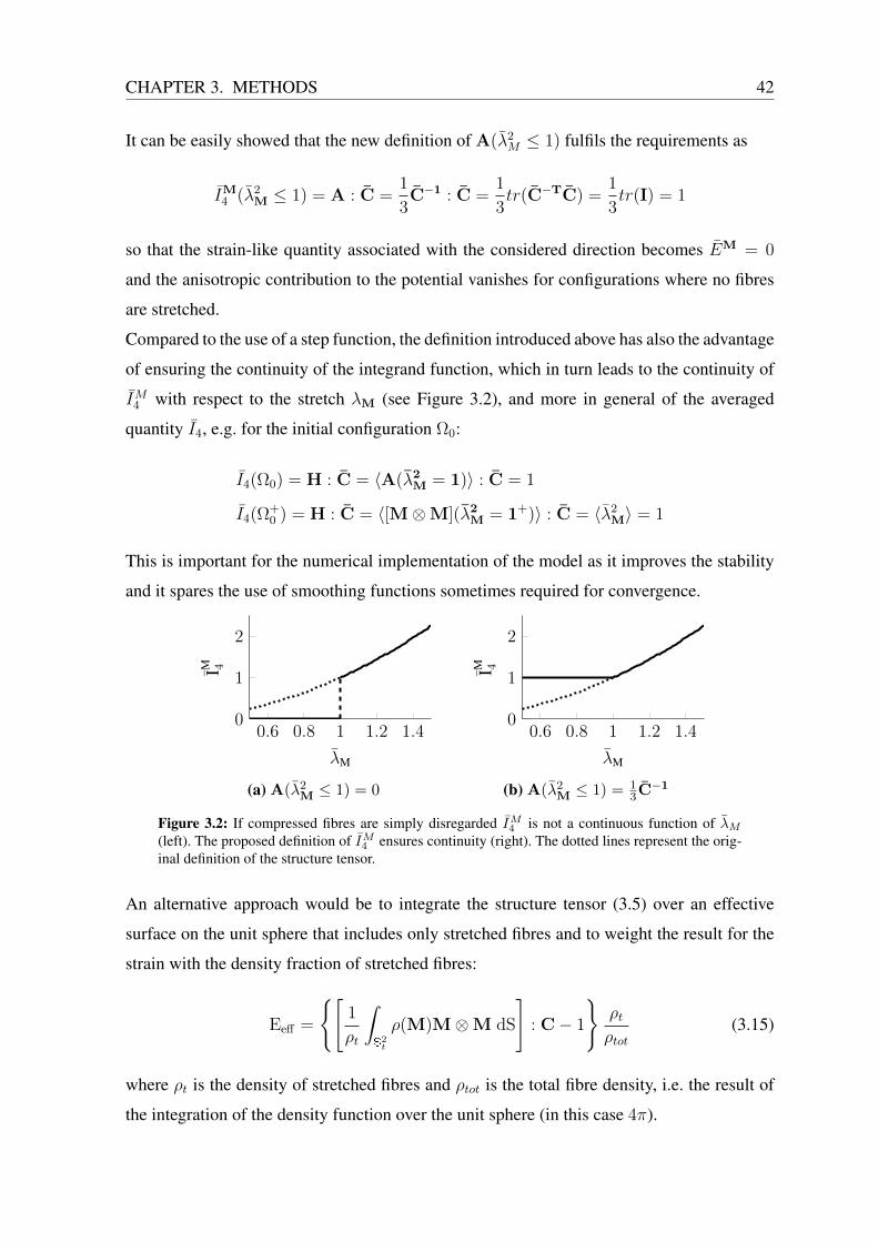
CHAPTER 3. METHODS 42
It can be easily showed that the new definition of A(λ2M ≤ 1) fulfils the requirements as
IM4 (λ2M ≤ 1) = A : C =
1
3C−1 : C =
1
3tr(C−TC) =
1
3tr(I) = 1
so that the strain-like quantity associated with the considered direction becomes EM = 0
and the anisotropic contribution to the potential vanishes for configurations where no fibres
are stretched.
Compared to the use of a step function, the definition introduced above has also the advantage
of ensuring the continuity of the integrand function, which in turn leads to the continuity of
IM4 with respect to the stretch λM (see Figure 3.2), and more in general of the averaged
quantity I4, e.g. for the initial configuration Ω0:
I4(Ω0) = H : C = 〈A(λ2M = 1)〉 : C = 1
I4(Ω+0 ) = H : C = 〈[M⊗M](λ2M = 1+)〉 : C = 〈λ2
M〉 = 1
This is important for the numerical implementation of the model as it improves the stability
and it spares the use of smoothing functions sometimes required for convergence.
0.6 0.8 1 1.2 1.40
1
2
λM
IM 4
(a) A(λ2M ≤ 1) = 0
0.6 0.8 1 1.2 1.40
1
2
λM
IM 4
(b) A(λ2M ≤ 1) = 1
3C−1
Figure 3.2: If compressed fibres are simply disregarded IM4 is not a continuous function of λM(left). The proposed definition of IM4 ensures continuity (right). The dotted lines represent the orig-inal definition of the structure tensor.
An alternative approach would be to integrate the structure tensor (3.5) over an effective
surface on the unit sphere that includes only stretched fibres and to weight the result for the
strain with the density fraction of stretched fibres:
Eeff =
[1
ρt
∫S2t
ρ(M)M⊗M dS
]: C− 1
ρtρtot
(3.15)
where ρt is the density of stretched fibres and ρtot is the total fibre density, i.e. the result of
the integration of the density function over the unit sphere (in this case 4π).
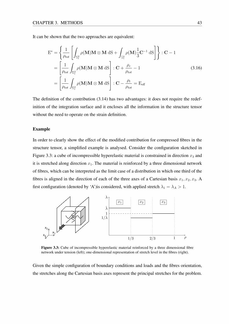
CHAPTER 3. METHODS 43
It can be shown that the two approaches are equivalent:
E∗ =
1
ρtot
[∫S2t
ρ(M)M⊗M dS +
∫S2c
ρ(M)1
3C−1 dS
]: C− 1
=
[1
ρtot
∫S2t
ρ(M)M⊗M dS
]: C +
ρcρtot− 1
=
[1
ρtot
∫S2t
ρ(M)M⊗M dS
]: C− ρt
ρtot= Eeff
(3.16)
The definition of the contribution (3.14) has two advantages: it does not require the redef-
inition of the integration surface and it encloses all the information in the structure tensor
without the need to operate on the strain definition.
Example
In order to clearly show the effect of the modified contribution for compressed fibres in the
structure tensor, a simplified example is analysed. Consider the configuration sketched in
Figure 3.3: a cube of incompressible hyperelastic material is constrained in direction x3 and
it is stretched along direction x1. The material is reinforced by a three dimensional network
of fibres, which can be interpreted as the limit case of a distribution in which one third of the
fibres is aligned in the direction of each of the three axes of a Cartesian basis x1, x2, x3. A
first configuration (denoted by ‘A’)is considered, with applied stretch λ1 = λA > 1.
ρ1/3 2/3 1
λ
1/λ1
λ
x1 x2 x3
Figure 3.3: Cube of incompressible hyperelastic material reinforced by a three dimensional fibrenetwork under tension (left); one-dimensional representation of stretch level in the fibres (right).
Given the simple configuration of boundary conditions and loads and the fibres orientation,
the stretches along the Cartesian basis axes represent the principal stretches for the problem.
CHAPTER 3. METHODS 44
Hence, the deformation gradient is simply given by the diagonal matrix:
F =
λ1 0 0
0 λ2 0
0 0 λ3
(3.17)
Incompressibility prevents volume changes. According to (2.7) this can be expressed as
J = det(F) = λ1λ2λ3 = 1 (3.18)
which immediately leads to the stretch in direction x2
λ2 =1
λ1λ3
=1
λA(3.19)
where λ1 = λA and λ3 = 1 due to the constraint in direction x3.
Assuming perfect bonding between fibres and matrix, the principal stretches can be directly
associated to the fibres in the corresponding direction. The stretch level in the fibres can
therefore be schematically represented as in Figure 3.3. Clearly, only the fibres in direction
x1 are stretched, and therefore they are the only ones that should contribute to the energy,
such that Ψ = f(E1), where E1 = λ21 − 1 is a measure of the strain in direction x1, defined
in analogy with E.
Using an approach similar to the one described in section 3.1, the averaged squared stretch
(corresponding to H : C) is used to compute the fibre contribution to the energy through the
strain measure E = 〈λ2〉 − 1.
The calculations are performed (i) according to the definition of H as in (3.5), (ii) applying
the Heaviside function to eliminate the contribution of the compressed fibres and (iii) modi-
fying H as described above in this section. The results are, respectively:
EA = λ2A
1
3+ 1 · 1
3+
1
λ2A
1
3− 1 =
(λ2A − 1)2
3λ2A
EHA = λ2
A
1
3− 1
E∗A = λ2A
1
3+
2
3− 1 =
λ2A − 1
3
(3.20)
A second configuration (denoted by ‘B’) is then considered, in which the stretch λ1 is such
CHAPTER 3. METHODS 45
that the strain in direction x1 is k times the corresponding strain in configuration (A) with
k > 1, i.e.
EB1 = kEA
1 ⇒ λB1 = λB =√kλ2
A − k + 1 (3.21)
The energy contribution in this configuration is then expected to be ΨB = f(EB1 ) = f(kEA
1 ).
Once again the averaged squared stretch is used to compute the energy associated with this
configuration. The results for the three cases defined above are
EB =kλ2
A − k + 1
3+
1
3+
1
3(kλ2A − k + 1)
− 1 = . . .
=λ2Ak
2
λ2Ak − k + 1
(λ2A − 1)2
3λ2A
=λ2Ak
2
λ2B
EA
EHB =
kλ2A − k + 1
3− 1 = k(
λ2A
3− 1) +
2
3(k − 1) = kEH
A −2
3(k − 1)
E∗B =kλ2
A − k + 1
3− 1
3= k
λ2A − 1
3= kE∗A
(3.22)
The comparison of the results for the two configurations shows that only the modification
described in this work leads to the correct representation of the energy contribution. In par-
ticular the original definition of λ2 is such that the change in the compression of the fibres in
direction x2 (that should not influence the energy) modulates the change of the strain mea-
sure, whereas the introduction of the Heaviside function alters the expected energy contri-
bution with a term related to the change of strain in the stretched fibres direction. Moreover,
it should be noted that the potential defined in (3.11) is a quadratic function of the strain-
like quantity E, so that Ψ(E) = Ψ(|E|). Thus, the introduction of the Heaviside function
results in a clearly non-physical behaviour for all the cases where kλ <√
3, since the con-
tribution for configuration (B), where the fibres are more stretched, is lower than the one for
configuration (A):
|EHA | = −EH
A ⇒ |EHB | = k|EH
A | −2
3(k − 1) (3.23)
where 2/3(k − 1) is always positive as k > 1.
Finally, the example confirms that the approach suggested in this work provides the same re-
sults as an effective strain computed through the average of the stretch only over an effective
area on the spherical surface (in this limit case direction x1) and weighted with the density
CHAPTER 3. METHODS 46
fraction of the stretched fibres (in this case 1/3):
Eeff = (λ2 − 1) · 1
3=λ2 − 1
3= E∗A (3.24)
Once again it is emphasized that the problem analysed above is indeed a strong simplification
of the case considered in this work and cannot be directly assumed as a general proof of the
correct behaviour of the model proposed here, but it serves the purpose of clearly showing
the advantages of the chosen approach with respect to other possible solutions.
3.2.2 Viscoelastic contribution
The viscoelastic response was modelled using the concept of internal variables described in
section 2.5, i.e. as the superposition of an elastic equilibrium response and a number of non-
equilibrium viscous processes. Accordingly, it was assumed that viscoelasticity is associated
only with the isochoric part of the deformation, as it is well established in the literature (see
[25] for a complete discussion).
Moreover, since it has been observed also in tensile tests, where fluid pressure is negligible
as well as the contribution from the proteoglycan matrix (see section 1.2), the intrinsic vis-
coelasticity of AC must be mainly determined by the collagen fibres and their cross-links.
Hence, in the current work collagen fibres are considered viscoelastic, but the matrix is elas-
tic similarly to [34].
Finally, following [21] the viscoelastic potentials Ψα were expressed as a function of the
isochoric elastic strain-energy Ψ∞, which is responsible for the equilibrium response at t→∞:
Ψα(C) = β∞α Ψ∞(C) , α = 1, . . . ,m (3.25)
where β∞α ∈ [0,∞) are non-dimensional strain energy factors associated with τα.
In accordance with the assumptions above, the complete form of the isochoric potential en-
ergy reads
Ψ = Ψg(C) + (1 +m∑α=1
β∞α )[Ψ∞fi (C) + Ψ∞fa(C,H)] (3.26)
where the non-dimensional constant β∞α ∈ [0,∞) relates the elastic and the viscous repre-
sentations. It should be noted that this assumption is only valid close to the thermodynamic
equilibrium.
CHAPTER 3. METHODS 47
This relation is immediately extended to the stress tensors, leading to the following rate
equation for the viscous over-stress
˙SV
α +SVατα
= β∞α [ ˙S∞fi
+ ˙S∞fa ] = β∞α
˙S∞f (3.27)
Disregarding an instantaneous stress response at t = 0, the closed form solution of equation
(3.27) is given by the convolution integral [52]
SVα = β∞α
∫ T=t
T=0
exp
−(t− T )
τα
˙S∞f dT (3.28)
The integral (3.28) describes the viscous over-stress related to a α-relaxation process with
relaxation time τα ∈ (0,∞), and corresponds to the contribution of a single element in the
generalized Maxwell model, which is the most general representation for the linear case.
This approach takes into account that the relaxation does not occur at a single time, but at a
distribution of times. It is possible to define as many relaxation processes (i.e. spring-dashpot
elements in the Maxwell model) as are necessary to accurately represent the distribution. In
this work three elements were defined, as in many cases this is sufficient to approximate
correctly the time dependent behaviour shown by AC in experimental tests [35] [58].
As explained in section 2.5, the relation (3.28) defines a quasi-linear viscoelastic model,
which implies that in a relaxation test the relaxation function (i.e. stress normalized on the
maximum stress at the end of the loading ramp) is independent of the level of applied de-
formation. Experimental tests on AC have shown that this assumption is not verified [2], in-
dicating that a non-linear viscoelastic model is necessary to fully capture the time evolution
of the mechanical response. However, the superposition of an elastic matrix and a quasi-
linear viscoelastic reinforcement leads to a non-linear viscoelastic response for the tissue, as
was suggested in [62] for a mixture of quasi-linear viscoelastic components characterized by
different relaxation functions.
Following [62], it is possible to illustrate this effect considering the special case of stress
relaxation under a uniaxial loading condition along the longitudinal direction parallel to the
collagen fibre. At any given time t during the relaxation period it is possible to define the
relaxation ratio as the ratio between the stress at time t and the stress at the end of the
loading ramp, which equals the elastic solution for the limit case of a step load. Expressing
the stress carried by the fibre as a fraction of the stress borne by the matrix dependent on the
CHAPTER 3. METHODS 48
strain level, the total relaxation ratio reads:
R(t) =σ
(t)m + σ
(t)f
σem + σef=σef = α(ε)σem
=
σ(t)m + σ
(t)f
σem(1 + α(ε))(3.29)
Having assumed that only the fibres are viscoelastic, it is possible to define different relax-
ation ratios for the components, and in particular to set R(t)m = 1:
σ(t)m = R(t)
m σem = σem ; σ
(t)f = R
(t)f σ
ef = R
(t)f α(ε)σem (3.30)
Finally, substituting (3.30) into (3.29), it is possible to write the total relaxation ratio as a
function of the strain:
R(t)(ε) =σem + R
(t)f α(ε)σem
σem(1 + α(ε))=
1 + R(t)f α(ε)
1 + α(ε)(3.31)
which defines a non-linear viscoelastic behaviour.
At low strain levels, where the response is dominated by the matrix, the viscoelastic effect is
low, while it progressively increases to higher strain levels where more fibres are active and
the load is mostly carried by collagen.
3.3 Illustrative fibre distribution
In this section the specific probability function used in this work to describe the distribution
of collagen fibres in AC is introduced.
Following the procedure proposed in [13] [9] the π-periodic von Mises distributions ρ(Θ)
centred at Θ = π/2 and Θ = 0 were considered:
ρA
(Θ;
π
2, b)
=exp[b cos(2Θ− π)]
2πI0(b)(3.32a)
ρB(Θ; 0, b) =exp[b cos(2Θ)]
2πI0(b)(3.32b)
where b > 0 is a concentration parameter describing the dispersion about the polar axis (see
Figure 3.4 ) and I0 denotes the modified Bessel function of the first kind of order zero, given
by
I0(b) =1
π
∫ π
0
exp(b cos Θ) dΘ (3.33)
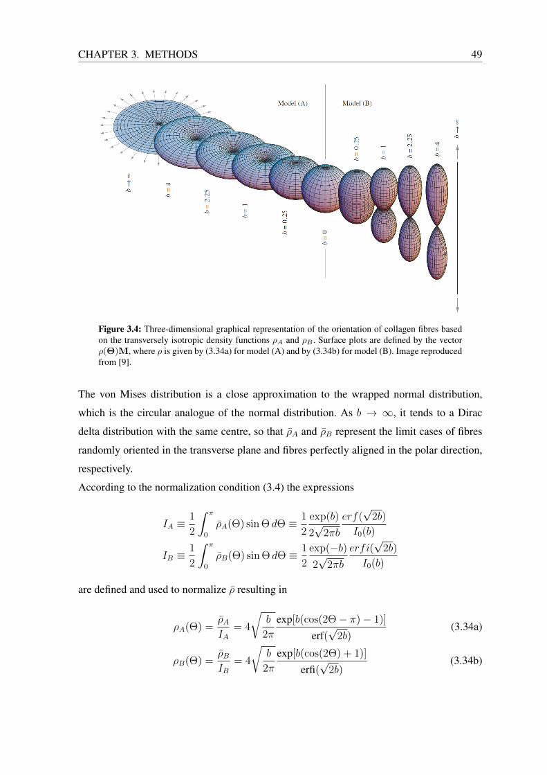
CHAPTER 3. METHODS 49
Figure 3.4: Three-dimensional graphical representation of the orientation of collagen fibres basedon the transversely isotropic density functions ρA and ρB . Surface plots are defined by the vectorρ(Θ)M, where ρ is given by (3.34a) for model (A) and by (3.34b) for model (B). Image reproducedfrom [9].
The von Mises distribution is a close approximation to the wrapped normal distribution,
which is the circular analogue of the normal distribution. As b → ∞, it tends to a Dirac
delta distribution with the same centre, so that ρA and ρB represent the limit cases of fibres
randomly oriented in the transverse plane and fibres perfectly aligned in the polar direction,
respectively.
According to the normalization condition (3.4) the expressions
IA ≡1
2
∫ π
0
ρA(Θ) sin Θ dΘ ≡ 1
2
exp(b)
2√
2πb
erf(√
2b)
I0(b)
IB ≡1
2
∫ π
0
ρB(Θ) sin Θ dΘ ≡ 1
2
exp(−b)2√
2πb
erfi(√
2b)
I0(b)
are defined and used to normalize ρ resulting in
ρA(Θ) =ρAIA
= 4
√b
2π
exp[b(cos(2Θ− π)− 1)]
erf(√
2b)(3.34a)
ρB(Θ) =ρBIB
= 4
√b
2π
exp[b(cos(2Θ) + 1)]
erfi(√
2b)(3.34b)
CHAPTER 3. METHODS 50
where erfi(x) = −ierf(x) is the imaginary error function [65], the error function itself being
erfi(x) =2√π
∫ π
0
exp(−t2) dt
The density functions (3.34) can be interpreted as a projection of the normal distribution onto
the unit sphere [10]. A graphical representation of the density functions (3.34) is provided
in Figure 3.4, in which the surface defined by the apex of the vector ρ(M)M is plotted with
respect to the Eulerian angles Θ and Φ. Note that for both the distributions b→ 0 represents
isotropy.
Due to the symmetry about the polar axis, the density functions (3.34) can also be represented
by means of a two-dimensional plot, which is frequently used in the literature to present his-
tological data, e.g. experimentally determined collagen distributions for planar collagenous
tissues [50].
It is important to note that using this approach it is only necessary to know the orientation of
the fibres in the reference configuration, since the new orientation in the current configuration
is given by the push forward of the reference direction (m = FM).
3.4 Spatial isochoric structure tensor
The solution of the governing equations is computed in an Eulerian setting. Hence, to in-
clude the structure tensor (3.5) in the numerical implementation, it is necessary to derive the
corresponding expression in the spatial reference.
The spatial isochoric fibre direction can be computed as the push-forward of M through the
isochoric deformation (χ∗[·]):
m = χ∗[M] = J−1/3FM = FM (3.35)
Similarly, the spatial isochoric structure tensor related to the fibre bundle in direction M
becomes
a = χ∗[M⊗M] = J−2/3F(M⊗M)FT = F(M⊗M)FT
= FM⊗ FTM = m⊗ m
(3.36)
which in turn leads to the following definition of the spatial isochoric averaged structure
CHAPTER 3. METHODS 51
tensor h
h = FHFT
=1
4π
∫S2
ρ(m)a(m) dS (3.37)
The trace of the spatial tensor a can be related to the stretch in direction M:
tr(a) := a : I = (m⊗ m) : I = m · m = FM · FM = (FTF) : (M⊗M)
= C : (M⊗M) = IM4 (C,M) = λ2M
(3.38)
Hence, the positivity of tr(a) can be used to check whether a fibre bundle is stretched. More-
over, the Green-Lagrange strain like quantity E can be written with respect to the spatial
configuration as
e = h : I− 1 (3.39)
Thus, in the spatial reference the correct modification of the structure tensor contribution in
direction m is given by
a∗ = FA∗FT
=
13I if tr(a) ≤ 1
m⊗ m if tr(a) > 1(3.40)
where the Eulerian contribution for compressed fibre corresponds to the isochoric push-
forward of the Lagrangian contribution:
χ∗[C−1
] = FC−1
FT = F(F−1
FT)FT = I (3.41)
3.5 Cauchy stress tensor and spatial elasticity tensor
Specific expressions for the stress and the elasticity tensors in the spatial configuration must
be derived to compute the numerical solution of the governing equations (see section 2.6).
This can be done introducing the particularized free-energy function defined in section 3.2
into the continuum mechanical framework discussed in chapter 2.
Given the decoupled form of the potential used in this work and the incompressibility as-
sumption, only the isochoric contribution needs to be considered. Moreover, the following
analysis is limited to the equilibrium stress and tangent elasticity tensors, as the viscous con-
tributions can be immediately computed as a function of the elastic results.
CHAPTER 3. METHODS 52
Firstly, the ground matrix is considered. It is convenient to introduce first and second deriva-
tive of the first isochoric invariant relative to the isochoric right Cauchy-Green tensor:
∂I1
∂C=∂(C : I)
∂C= I (3.42)
∂2I1
∂C2=∂(I)
∂C= O (3.43)
According to the definition of σ in (2.51) and the expression of the neo-Hookean potential
(3.7), the isochoric Cauchy stress associated with the matrix is given by
σ∞g = 2J−1F
[∂Ψg
∂C
]FT = 2J−1/3F
[c0
2I]
FT = J−1/3[c0b] (3.44)
σ∞g = J−2/3p : σ∞g = J−1p : [cob] (3.45)
where p is the deviatoric operator and b is the isochoric left Cauchy Green tensor defined in
(2.39).
Hence, the contribution to the elasticity tensor can be computed immediately, as the first
term in (2.81), i.e. J−4/3p : c : p, vanishes in accordance with the definition of c and the
result for the second derivative of the potential relative to the isochoric right Cauchy-Green
tensor (3.43), whereas the second and third terms 23J−2/3tr(σ)p and 2
3[I ⊗ σ + σ ⊗ I] are
directly computed from (3.44) and (3.45). These are well known result in the literature, see
for example [39] [13].
The same arguments can be used for the isotropic fibre contribution, which is also modelled
as a neo-Hookean material, simply substituting cfi to c0. Hence, the isochoric Cauchy stress
associated with the isotropic fibre contribution reads
σ∞fi = J−1p : [cfib] (3.46)
Once again, this expression leads directly to the expression for the elasticity tensor.
Similarly to [64] [9] the anisotropic fibre potential is assumed to be a function solely of
the Green-Lagrange strain like quantity E. According to the particularized expression of the
potential (3.11) it is then possible to compute the scalar quantities
ψ′fa =dΨ∞fadE
= cfaE (3.47)
CHAPTER 3. METHODS 53
ψ′′fa =d2Ψ∞fadE
= cfa (3.48)
Also, it is convenient to report the derivative of E with respect to C
∂E
∂C=∂(C : H− 1)
∂C= H (3.49)
Using the arguments in section 2.4.1 and the equations (3.47) (3.49)
∂Ψ∞fa∂C
=∂Ψ∞fa∂E
∂E
∂C= ψ′faH (3.50)
σ∞fa = 2ψ′faJ−1FHFT = 2ψ′faJ
−1/3FHFT
= 2ψ′faJ−1/3h (3.51)
where the spatial isochoric structure tensor h is introduced according to (3.37). Finally, the
isochoric Cauchy stress reads
σ∞fa = 2ψ′faJ−1p : h (3.52)
In order to particularize the expression of the spatial isochoric elasticity tensor, it is only
necessary to particularize the first part of (2.81), i.e. J−4/3p : c : p, as the contributions from
the second and third terms 23J−2/3tr(σ)p and 2
3[I⊗ σ+ σ⊗ I] can be obtained immediately
by using the results in (3.51) (3.52).
The second derivative of the anisotropic fibre potential relative to C is given by
∂2Ψ∞fa∂C2
=∂[ψ′faH]
∂C=∂ψ′fa∂E
∂E
∂C⊗H + ψ′fa
∂H
∂C= ψ′′faH⊗H (3.53)
where the derivative of the structure tensor H relative to C is assumed to be the null fourth
order tensor O. According to its definition, the structure tensor is indeed dependent on the
isochoric deformation that determines the amount of fibres that contribute to the potential.
Nevertheless, this is the correct assumption based on the numerical implementation of the
model (details are given in section 3.6).
According to the definition c∞ = J−1χ∗[4∂2Ψ/∂C2], the spatial isochoric (fictitious) elas-
ticity tensor is given by
[c]∞ijkl = 4J−1FiIFjJFkKFlL[ψ′′faH⊗H] = 4J1/3FiIFjJ FkKFlL[ψ′′faH⊗H]
= 4J1/3[ψ′′fah⊗ h](3.54)
CHAPTER 3. METHODS 54
Hence, the first contribution to the spatial isochoric elasticity tensor becomes
J−4/3p : c∞ : p = 4J−1ψ′′fa(p : h)⊗ (p : h) (3.55)
With the major and minor symmetries of the elasticity tensor (see section 2.6) contributions
accounted for, these relations can be efficiently implemented into a finite element code.
3.6 Numerical implementation
Due to complex geometries, material properties and loading conditions, in general it is not
possible to find an analytical solution for the model presented in the previous sections and
numerical methods are required. In this section the numerical implementation of the model
is analysed, with focus on the assumptions and procedures adopted to solve the equations in
the framework of Finite Element Analysis.
The Finite Element Method has proven to be particularly effective in the modelling of bio-
logical tissues and has been used routinely in the literature. A description of this method is
out of the scope of this work and for a detailed discussion the reader is referred to [69]. The
general purpose finite element package FEAP1 was chosen to perform the analysis since it
allows the use of custom materials through user-defined subroutines and it has been reported
to be effective in modelling soft biological tissues [13] [21] and also specifically AC [9].
3.6.1 Structure tensor
To implement the structure tensor defined in (3.37), it is necessary to evaluate the strain in
all directions for every integration point in each element of the mesh.
The system of non-linear equation representing the problem cannot be solved directly, but
some iterative procedure is required. At each solution step a number of linearised sub-steps
is performed until converged solution is achieved (see section 3.7.2). The deformation is
computed at each sub step, so that the number and location of stretched collagen bundles
might change within the iterations.
This means that on the error reduction path towards a converged solution, the configuration of
stretched fibres (and therefore the associated anisotropic energy contribution) might suddenly
1FEAP-A Finite Element Analysis Program version 8.2. Berkeley, California: R. L. Taylor, 2008
CHAPTER 3. METHODS 55
change, so that the exact solution changes as well. Thus, the iterative method needs to start a
path towards the new solution.
Even if the solution of the previous sub-step (that is used as starting point for the new iterative
process) is likely to be in the so-called region of attraction of the new solution (i.e. to be
close enough to the new solution to prevent that the iterative method converges to a different
solution), every configuration change affects the rate of convergence and multiple changes
might prevent the achievement of a converged solution before the chosen maximum number
of iteration is reached.
Therefore, at each solution step the stretch is kept constant during the Newton iterations. In
particular, the value computed at the previous step is used, assuming that time and load vari-
ations are small enough to make the difference negligible. The check is anyway performed
at each sub-step and the value of IM4 computed at the last sub-step (i.e. the one that gives
converged solution) is then use at the next solution step. This approach is not ideal, as it
requires the definition of history variables to store the stretch information when the solution
is updated.
On the other hand, as mentioned in section 3.5, it simplifies the derivation of stress and elas-
ticity tensor. The structure tensor H is not independent of the right Cauchy-Green tensor
C because the deformation determines the number and position of fibres bundles that are
stretched at a particular solution step. However, at each the step n the derivation of the en-
ergy function Ψ is relative to the current deformation state (i.e. Cn), but the value of Hn−1
of the previous step is used, which is indeed dependent on the deformation up to Cn−1 but
constant with respect to Cn.
3.6.2 Spherical integration
Following [9], the structure tensor (3.5) was integrated using a spherical t-design, consisting
of a set of N points on the unit sphere M(1), . . . ,M(N) ∈ S2 (i.e. a set of N directions),
such that, as S(S2) = 4π is the surface measure of the unit sphere in R3, the equality
∫S2
f(M) dS =4π
N
N∑α=1
f(A(α)) (3.56)

CHAPTER 3. METHODS 56
holds for polynomials f of degree k ≤ t [17]. Hence, using (3.5) the structure tensor can be
computed as
H =1
N
N∑α=1
ρ(M(α))A(α) (3.57)
The degree t required to guarantee the desired precision depends on the form of the proba-
bility density function ρ. Therefore, in the case of the transversely isotropic distribution used
in this work, the integration order is defined by the concentration parameter b, that has a
specific value for each element. In particular t should be increased as b increases, i.e. when
the fibres are more concentrated about the polar axis.
Indeed, it would be possible to define an empirical relation between b and t as in [9] [15] and
to set the order in each element depending on its value of b. In this work though the same
order was used for all the elements, as the corresponding number of points N on the unit
sphere was necessary to initialize the history variables required to store the value of IM4 at
each solution step, which are globally defined for all the elements. Numerical compression
experiments were performed increasing t until convergence was achieved and the minimum
sufficient value was found to be t = 21, corresponding to the N = 240 integration points2
plotted in Figure 3.5.
Figure 3.5: Graphical representation of the spherical t-design with t = 21, corresponding to 240points on the unit sphere.
It should be noted that increasing the order of the spherical integration also increases the
size of the problem and the computational cost: for every additional integration point on the
unit sphere (note that the number of points required for a one-order improvement increases
with t), a total of n × gp new operations are required to compute the structure tensor, and
n × gp new history variables need to be stored, where n is the number of elements in the
2The coordinates of all the points are reported at http://neilsloane.com/sphdesigns/
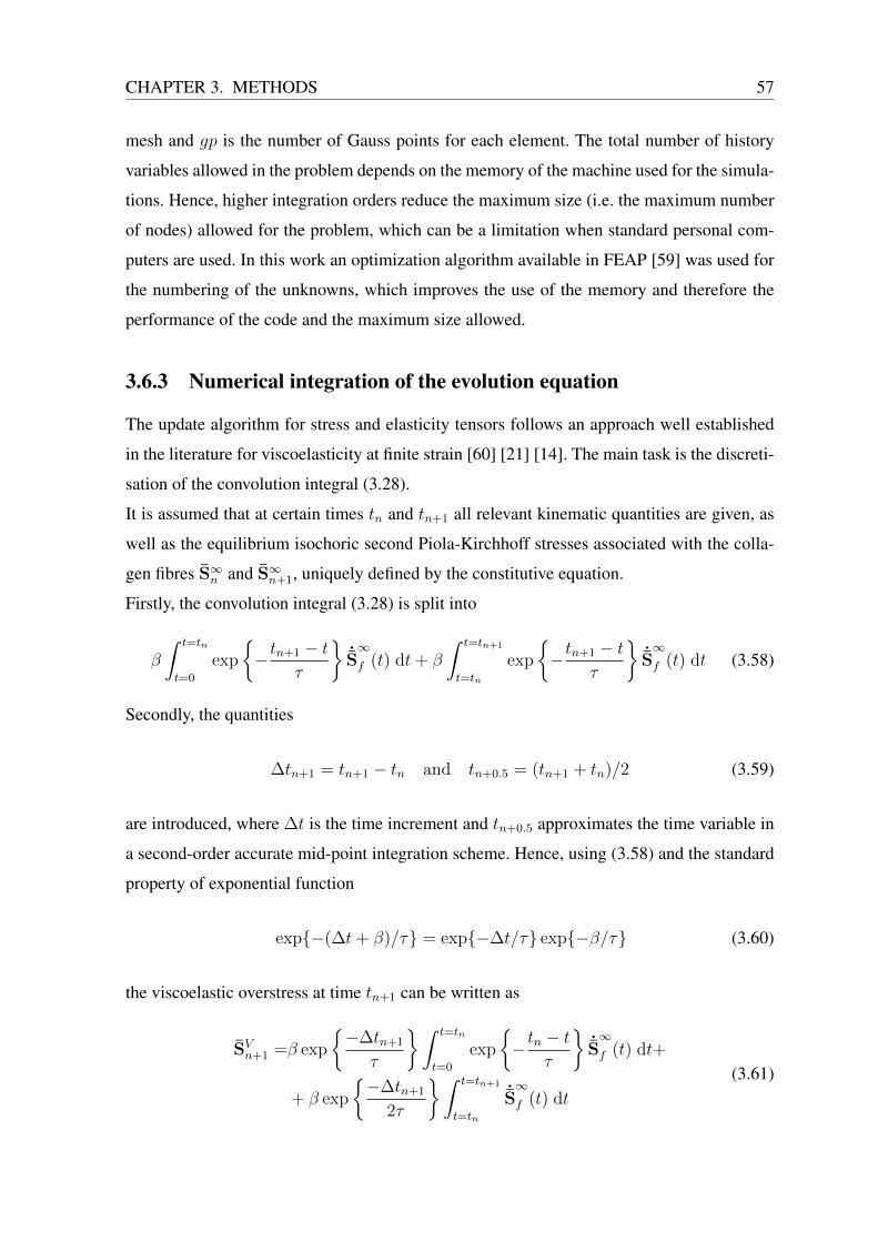
CHAPTER 3. METHODS 57
mesh and gp is the number of Gauss points for each element. The total number of history
variables allowed in the problem depends on the memory of the machine used for the simula-
tions. Hence, higher integration orders reduce the maximum size (i.e. the maximum number
of nodes) allowed for the problem, which can be a limitation when standard personal com-
puters are used. In this work an optimization algorithm available in FEAP [59] was used for
the numbering of the unknowns, which improves the use of the memory and therefore the
performance of the code and the maximum size allowed.
3.6.3 Numerical integration of the evolution equation
The update algorithm for stress and elasticity tensors follows an approach well established
in the literature for viscoelasticity at finite strain [60] [21] [14]. The main task is the discreti-
sation of the convolution integral (3.28).
It is assumed that at certain times tn and tn+1 all relevant kinematic quantities are given, as
well as the equilibrium isochoric second Piola-Kirchhoff stresses associated with the colla-
gen fibres S∞n and S∞n+1, uniquely defined by the constitutive equation.
Firstly, the convolution integral (3.28) is split into
β
∫ t=tn
t=0
exp
−tn+1 − t
τ
˙S∞f (t) dt+ β
∫ t=tn+1
t=tn
exp
−tn+1 − t
τ
˙S∞f (t) dt (3.58)
Secondly, the quantities
∆tn+1 = tn+1 − tn and tn+0.5 = (tn+1 + tn)/2 (3.59)
are introduced, where ∆t is the time increment and tn+0.5 approximates the time variable in
a second-order accurate mid-point integration scheme. Hence, using (3.58) and the standard
property of exponential function
exp−(∆t+ β)/τ = exp−∆t/τ exp−β/τ (3.60)
the viscoelastic overstress at time tn+1 can be written as
SVn+1 =β exp
−∆tn+1
τ
∫ t=tn
t=0
exp
−tn − t
τ
˙S∞f (t) dt+
+ β exp
−∆tn+1
2τ
∫ t=tn+1
t=tn
˙S∞f (t) dt
(3.61)
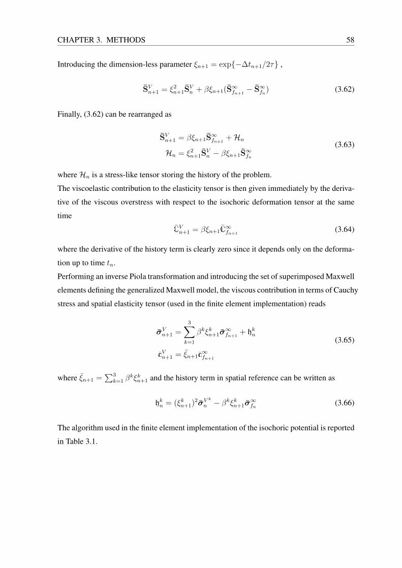
CHAPTER 3. METHODS 58
Introducing the dimension-less parameter ξn+1 = exp−∆tn+1/2τ ,
SVn+1 = ξ2n+1S
Vn + βξn+1(S∞fn+1
− S∞fn) (3.62)
Finally, (3.62) can be rearranged as
SVn+1 = βξn+1S∞fn+1
+Hn
Hn = ξ2n+1S
Vn − βξn+1S
∞fn
(3.63)
whereHn is a stress-like tensor storing the history of the problem.
The viscoelastic contribution to the elasticity tensor is then given immediately by the deriva-
tive of the viscous overstress with respect to the isochoric deformation tensor at the same
time
CVn+1 = βξn+1C∞fn+1
(3.64)
where the derivative of the history term is clearly zero since it depends only on the deforma-
tion up to time tn.
Performing an inverse Piola transformation and introducing the set of superimposed Maxwell
elements defining the generalized Maxwell model, the viscous contribution in terms of Cauchy
stress and spatial elasticity tensor (used in the finite element implementation) reads
σVn+1 =3∑
k=1
βkξkn+1σ∞fn+1
+ hkn
cVn+1 = ξn+1c∞fn+1
(3.65)
where ξn+1 =∑3
k=1 βkξkn+1 and the history term in spatial reference can be written as
hkn = (ξkn+1)2σVk
n − βkξkn+1σ∞fn (3.66)
The algorithm used in the finite element implementation of the isochoric potential is reported
in Table 3.1.
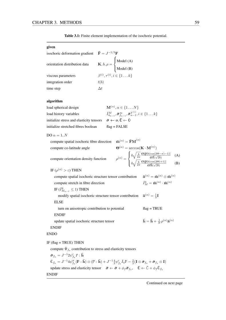
CHAPTER 3. METHODS 59
Table 3.1: Finite element implementation of the isochoric potential.
given
isochoric deformation gradient F = J−1/3F
orientation distribution data K, b, ρ =
Model (A)
Model (B)
viscous parameters β(i), τ (i), i ∈ 1 . . . kintegration order t(b)
time step ∆t
algorithm
load spherical design M(α), α ∈ 1 . . . Nload history variables IM4n−1
, σ∞fn−1, σV
(i)
n−1, i ∈ 1 . . . kinitialize stress and elasticity tensors σ← o, C← O
initialize stretched fibres boolean flag = FALSE
DO α = 1, N
compute spatial isochoric fibre direction m(α) = FM(α)
compute co-latitude angle Θ(α) = arccos(K ·M(α))
compute orientation density function ρ(α) =
4√
b2π
exp[b(cos(2Θ−π)−1)]
erf(√2b)(A)
4√
b2π
exp[b(cos(2Θ)+1)]
erfi(√
2b)(B)
IF (ρ(α) > ε) THEN
compute spatial isochoric structure tensor contribution a(α) = m(α) ⊗ m(α)
compute stretch in fibre direction I4M = m(α) · m(α)
IF (I4Mn−1
≤ 1) THEN
modify spatial isochoric structure tensor contribution a(α) = 13I
ELSE
turn on anisotropic contribution to potential flag = TRUE
ENDIF
update spatial isochoric structure tensor h = h + 1N ρ
(α)a(α)
ENDIF
ENDO
IF (flag = TRUE) THEN
compute Ψfa contribution to stress and elasticity tensors
σfa = J−12ψ′faP : h
Cfa = J−14ψ′′fa(P : h)⊗ (P : h) + J−1 43ψ′faI4P− 2
3 (I⊗ σfa + σfa ⊗ I)
update stress and elasticity tensor σ ← σ + φf σfa , C← C+ φf Cfa
ENDIF
Continued on next page
CHAPTER 3. METHODS 60
Table 3.1: (continued)
add Ψfi contribution to stress and elasticity tensors (neo-hookean)
σ ← σ + φf σfi
C← C+ φf Cfi
store elastic fibre contribution σ∞f ← σ
DO i = 1, k
compute viscous parameters
ξ(i) = exp[−∆t/2τ (i)]
ξ ← ξ + ξ(i)
compute viscous overstress
σV(i)
= β(i)ξ(i)σ + [(ξ(i))2σV(i)
n−1 − β(i)ξ(i)σ∞fn−1]
σV ← σV + σV(i)
ENDDO
compute viscous contribution to elasticity tensor CV = ξC
update stress and elasticity tensor σ ← σ+ σV , C← C+ CV
add Ψg contribution to stress and elasticity tensors (neo-hookean)
σ ← σ + φgσg
C← C+ φgCg
history update (if converged solution is achieved)
I4M → I4
Mn−1
σ∞f → σ∞fn−1
σV(i) → σV
(i)
n−1
3.7 Representative numerical examples
Three numerical examples were analysed to demonstrate the physical behaviour of the con-
stitutive relations defined above3. Experimental studies selected from the literature were used
to validate the results. In this section these examples and the solution procedure adopted are
discussed in details.
The probability density function defined in 3.3 was used in the example studies and the
concentration parameter b was changed linearly across the thickness. In a full-thickness
3All the computations were performed on a standard personal computer (Dell optiplex GX790).
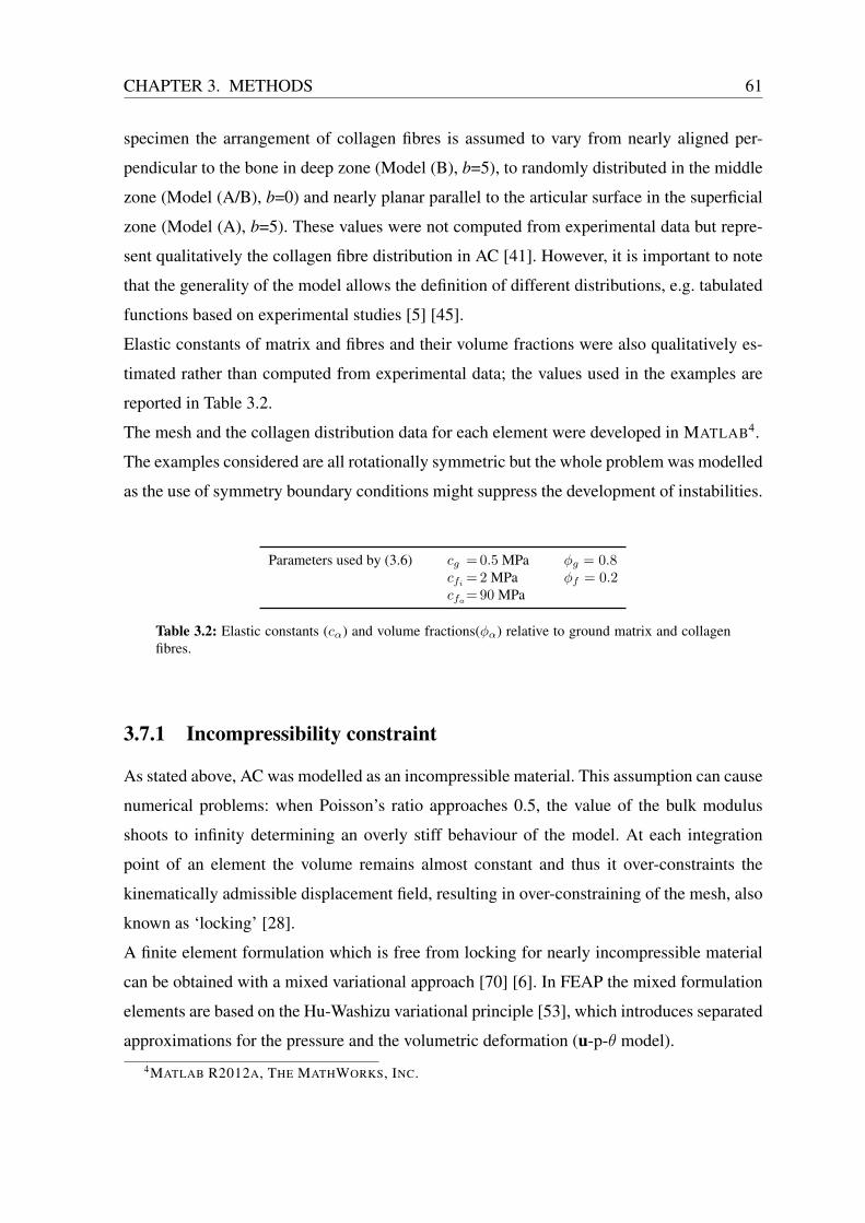
CHAPTER 3. METHODS 61
specimen the arrangement of collagen fibres is assumed to vary from nearly aligned per-
pendicular to the bone in deep zone (Model (B), b=5), to randomly distributed in the middle
zone (Model (A/B), b=0) and nearly planar parallel to the articular surface in the superficial
zone (Model (A), b=5). These values were not computed from experimental data but repre-
sent qualitatively the collagen fibre distribution in AC [41]. However, it is important to note
that the generality of the model allows the definition of different distributions, e.g. tabulated
functions based on experimental studies [5] [45].
Elastic constants of matrix and fibres and their volume fractions were also qualitatively es-
timated rather than computed from experimental data; the values used in the examples are
reported in Table 3.2.
The mesh and the collagen distribution data for each element were developed in MATLAB4.
The examples considered are all rotationally symmetric but the whole problem was modelled
as the use of symmetry boundary conditions might suppress the development of instabilities.
Parameters used by (3.6) cg = 0.5 MPa φg = 0.8cfi = 2 MPa φf = 0.2cfa= 90 MPa
Table 3.2: Elastic constants (cα) and volume fractions(φα) relative to ground matrix and collagenfibres.
3.7.1 Incompressibility constraint
As stated above, AC was modelled as an incompressible material. This assumption can cause
numerical problems: when Poisson’s ratio approaches 0.5, the value of the bulk modulus
shoots to infinity determining an overly stiff behaviour of the model. At each integration
point of an element the volume remains almost constant and thus it over-constraints the
kinematically admissible displacement field, resulting in over-constraining of the mesh, also
known as ‘locking’ [28].
A finite element formulation which is free from locking for nearly incompressible material
can be obtained with a mixed variational approach [70] [6]. In FEAP the mixed formulation
elements are based on the Hu-Washizu variational principle [53], which introduces separated
approximations for the pressure and the volumetric deformation (u-p-θ model).
4MATLAB R2012A, THE MATHWORKS, INC.
CHAPTER 3. METHODS 62
For the present study the Q1-P0 element available in FEAP was used, which is a large de-
formation finite element based on the Hu-Washizu variational formulation. It uses linear
shape functions for the deformation field related to the deviatoric kinematical variables and
constant ansatz functions to discretise the pressure and volumetric strain. The volumetric
variables are eliminated on the element level.
Finite elements that are derived from mixed methods have to fulfil the so-called BB-condition
to guarantee the stability of the formulation [68]. The Q1-P0 element does not fulfil this con-
dition in the geometrical linear theory, which implies that it can generate unstable solution
for the pressure under particular loads or boundary conditions. Nevertheless, it has been ob-
served in many practical application that it is robust for finite elasticity problems involving
quasi-incompressible material, and therefore it is commonly used in commercial software.
Enforcing correctly the incompressibility constraint is also crucial to avoid non-physical
behaviour of the model when the decoupled form of the potential is used for fibre reinforced
composites [19].
This can be done using a penalty method. However, the use of large penalty parameters can
make the iterative method unable to converge. On the other hand, if the penalty parameter
value is reduced much in order to achieve convergence of the solution, the constraint is not
sufficiently enforced.
In the following examples, incompressibility was enforced using an augmented Lagrangian
solution strategy based on the Uzawa algorithm [70], which is available in FEAP. If a penalty
value vp is calculated from the equation
vp = K · c(u) (3.67)
where K is a material parameter and c(u) is a constraint to be made close to zero, then the
augmented Lagrangian parameter update is computed as
va = va + augf · vp. (3.68)
where augf is the augmentation factor. At each solution step, after a converged solution is
computed, the update is performed and the solution is computed again. The iteration con-
tinues until incompressibility is enforced up to a given tolerance of accuracy. Using this
solution the value of the penalty parameter has to be just one or two orders of magnitude
CHAPTER 3. METHODS 63
larger than the conventional stiffness terms, instead of the six or seven that are required in
the basic penalty method. This method is computationally expensive and the number of itera-
tions should be kept low. In order to do this, the augmentation factor can be increased as well
as the initial value of the bulk modulus. Numerical tests were performed with configurations
similar to the examples described below and finally two augmentation iterations were used
in the solution procedure.
3.7.2 Solution procedure
As mentioned above, the solution of a non-linear problem cannot be approached directly,
but some iterative procedure is required and the choice of a particular method is problem-
dependent. For the example problems studied in this work the Newton-Raphson method
was used, in which the asymptotic rate of convergence is quadratic. However, the numerical
solution can only approximately be achieved: since finite precision arithmetic is used in all
computer calculations, one can never achieve a better solution than the round-off limit of the
calculations. Hence, it is necessary to set some kind of tolerance on the solution to terminate
the iteration. Every iterative method aims to reduce the residual, which is defined as
R = KT∆U (3.69)
where KT is the stiffness matrix and ∆U is the displacement parameter change. Thus, it is
convenient to define the convergence criteria based on a norm of the residual, or similarly on
a norm of the energy, defined as
‖Ei‖ = (∆Ui ·Ri)1/2 (3.70)
In FEAP the energy of the first iteration in the current solution step is used as a basis and the
limit is expressed as some tolerance of its norm: ‖Ei‖ = ε‖E0‖, where ε is the tolerance.
Once a criterion is defined it is still necessary to choose an appropriate value for ε. The toler-
ance was chosen at half the machine precision (i.e. ε = 10−8), since quadratic convergence
assure that the next residual (disregarding round-off error) would achieve full precision.
It was observed that the rate the Newton-Raphson method did not achieve quadratic conver-
gence for relatively high level of compressive deformation, so that many iterations were nec-
essary to guarantee the chosen precision. This was not surprising as the progressive buckling
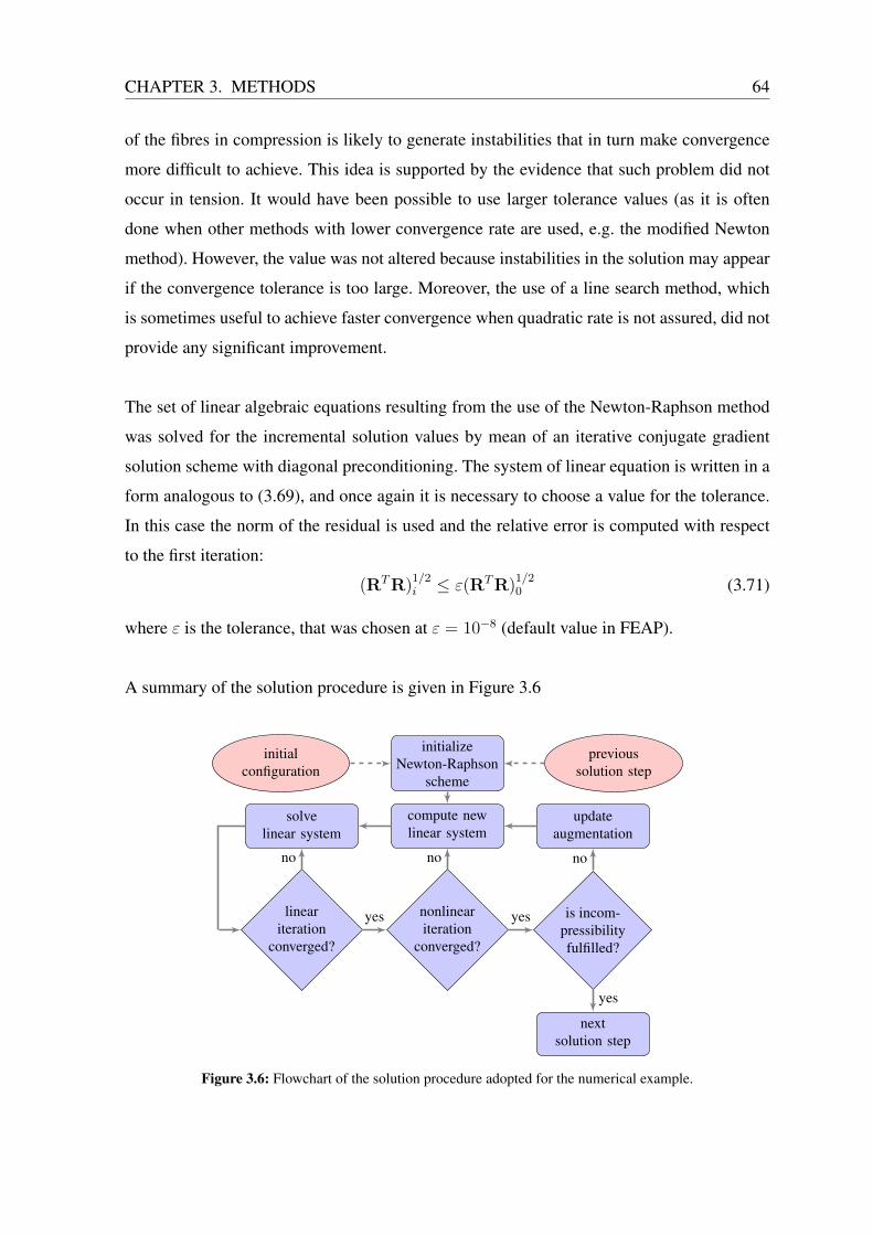
CHAPTER 3. METHODS 64
of the fibres in compression is likely to generate instabilities that in turn make convergence
more difficult to achieve. This idea is supported by the evidence that such problem did not
occur in tension. It would have been possible to use larger tolerance values (as it is often
done when other methods with lower convergence rate are used, e.g. the modified Newton
method). However, the value was not altered because instabilities in the solution may appear
if the convergence tolerance is too large. Moreover, the use of a line search method, which
is sometimes useful to achieve faster convergence when quadratic rate is not assured, did not
provide any significant improvement.
The set of linear algebraic equations resulting from the use of the Newton-Raphson method
was solved for the incremental solution values by mean of an iterative conjugate gradient
solution scheme with diagonal preconditioning. The system of linear equation is written in a
form analogous to (3.69), and once again it is necessary to choose a value for the tolerance.
In this case the norm of the residual is used and the relative error is computed with respect
to the first iteration:
(RTR)1/2i ≤ ε(RTR)
1/20 (3.71)
where ε is the tolerance, that was chosen at ε = 10−8 (default value in FEAP).
A summary of the solution procedure is given in Figure 3.6
initializeNewton-Raphson
scheme
initialconfiguration
previoussolution step
compute newlinear system
nonlineariteration
converged?
solvelinear system
updateaugmentation
lineariteration
converged?
is incom-pressibilityfulfilled?
nextsolution step
no
yes
no
yes
no
yes
Figure 3.6: Flowchart of the solution procedure adopted for the numerical example.
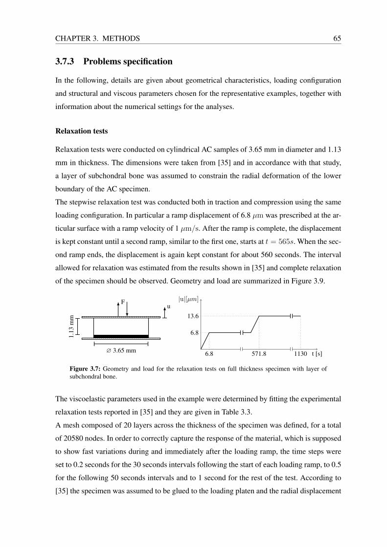
CHAPTER 3. METHODS 65
3.7.3 Problems specification
In the following, details are given about geometrical characteristics, loading configuration
and structural and viscous parameters chosen for the representative examples, together with
information about the numerical settings for the analyses.
Relaxation tests
Relaxation tests were conducted on cylindrical AC samples of 3.65 mm in diameter and 1.13
mm in thickness. The dimensions were taken from [35] and in accordance with that study,
a layer of subchondral bone was assumed to constrain the radial deformation of the lower
boundary of the AC specimen.
The stepwise relaxation test was conducted both in traction and compression using the same
loading configuration. In particular a ramp displacement of 6.8 µm was prescribed at the ar-
ticular surface with a ramp velocity of 1 µm/s. After the ramp is complete, the displacement
is kept constant until a second ramp, similar to the first one, starts at t = 565s. When the sec-
ond ramp ends, the displacement is again kept constant for about 560 seconds. The interval
allowed for relaxation was estimated from the results shown in [35] and complete relaxation
of the specimen should be observed. Geometry and load are summarized in Figure 3.9.
Fu
∅ 3.65 mm
1.13
mm
t [s]6.8 571.8 1130
|u|[µm]
6.8
13.6
Figure 3.7: Geometry and load for the relaxation tests on full thickness specimen with layer ofsubchondral bone.
The viscoelastic parameters used in the example were determined by fitting the experimental
relaxation tests reported in [35] and they are given in Table 3.3.
A mesh composed of 20 layers across the thickness of the specimen was defined, for a total
of 20580 nodes. In order to correctly capture the response of the material, which is supposed
to show fast variations during and immediately after the loading ramp, the time steps were
set to 0.2 seconds for the 30 seconds intervals following the start of each loading ramp, to 0.5
for the following 50 seconds intervals and to 1 second for the rest of the test. According to
[35] the specimen was assumed to be glued to the loading platen and the radial displacement
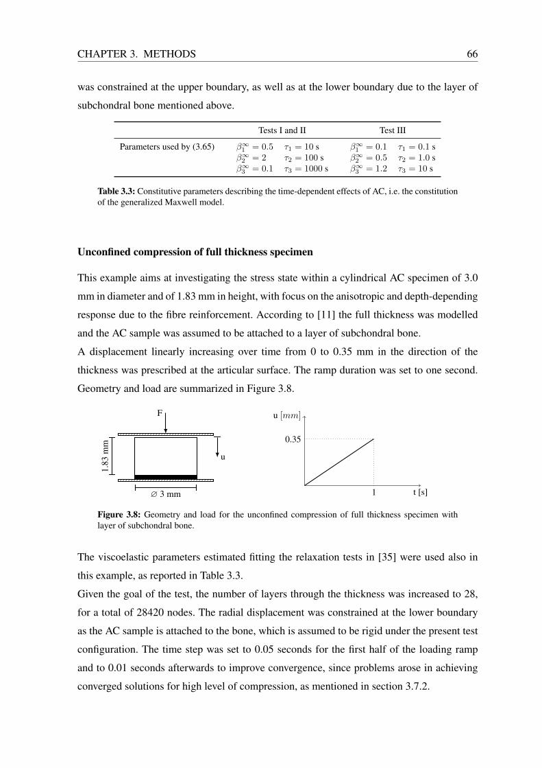
CHAPTER 3. METHODS 66
was constrained at the upper boundary, as well as at the lower boundary due to the layer of
subchondral bone mentioned above.
Tests I and II Test III
Parameters used by (3.65) β∞1 = 0.5 τ1 = 10 s β∞1 = 0.1 τ1 = 0.1 sβ∞2 = 2 τ2 = 100 s β∞2 = 0.5 τ2 = 1.0 sβ∞3 = 0.1 τ3 = 1000 s β∞3 = 1.2 τ3 = 10 s
Table 3.3: Constitutive parameters describing the time-dependent effects of AC, i.e. the constitutionof the generalized Maxwell model.
Unconfined compression of full thickness specimen
This example aims at investigating the stress state within a cylindrical AC specimen of 3.0
mm in diameter and of 1.83 mm in height, with focus on the anisotropic and depth-depending
response due to the fibre reinforcement. According to [11] the full thickness was modelled
and the AC sample was assumed to be attached to a layer of subchondral bone.
A displacement linearly increasing over time from 0 to 0.35 mm in the direction of the
thickness was prescribed at the articular surface. The ramp duration was set to one second.
Geometry and load are summarized in Figure 3.8.
F
u
∅ 3 mm
1.83
mm
t [s]1
u [mm]
0.35
Figure 3.8: Geometry and load for the unconfined compression of full thickness specimen withlayer of subchondral bone.
The viscoelastic parameters estimated fitting the relaxation tests in [35] were used also in
this example, as reported in Table 3.3.
Given the goal of the test, the number of layers through the thickness was increased to 28,
for a total of 28420 nodes. The radial displacement was constrained at the lower boundary
as the AC sample is attached to the bone, which is assumed to be rigid under the present test
configuration. The time step was set to 0.05 seconds for the first half of the loading ramp
and to 0.01 seconds afterwards to improve convergence, since problems arose in achieving
converged solutions for high level of compression, as mentioned in section 3.7.2.
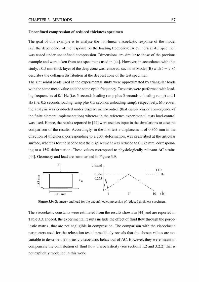
CHAPTER 3. METHODS 67
Unconfined compression of reduced thickness specimen
The goal of this example is to analyse the non-linear viscoelastic response of the model
(i.e. the dependence of the response on the loading frequency). A cylindrical AC specimen
was tested under unconfined compression. Dimensions are similar to those of the previous
example and were taken from test specimens used in [44]. However, in accordance with that
study, a 0.5 mm thick layer of the deep zone was removed, such that Model (B) with b = 2.85
describes the collagen distribution at the deepest zone of the test specimen.
The sinusoidal loads used in the experimental study were approximated by triangular loads
with the same mean value and the same cycle frequency. Two tests were performed with load-
ing frequencies of 0.1 Hz (i.e. 5 seconds loading ramp plus 5 seconds unloading ramp) and 1
Hz (i.e. 0.5 seconds loading ramp plus 0.5 seconds unloading ramp), respectively. Moreover,
the analysis was conducted under displacement-control (that ensure easier convergence of
the finite element implementation) whereas in the reference experimental tests load-control
was used. Hence, the results reported in [44] were used as input in the simulations to ease the
comparison of the results. Accordingly, in the first test a displacement of 0.366 mm in the
direction of thickness, corresponding to a 20% deformation, was prescribed at the articular
surface, whereas for the second test the displacement was reduced to 0.275 mm, correspond-
ing to a 15% deformation. These values correspond to physiologically relevant AC strains
[44]. Geometry and load are summarized in Figure 3.9.
F
u
∅ 3 mm
1.83
mm
t [s]1 5 10
u [mm]
0.3660.275
1 Hz0.1 Hz
Figure 3.9: Geometry and load for the unconfined compression of reduced thickness specimen.
The viscoelastic constants were estimated from the results shown in [44] and are reported in
Table 3.3. Indeed, the experimental results include the effect of fluid flow through the poroe-
lastic matrix, that are not negligible in compression. The comparison with the viscoelastic
parameters used for the relaxation tests immediately reveals that the chosen values are not
suitable to describe the intrinsic viscoelastic behaviour of AC. However, they were meant to
compensate the contribution of fluid flow viscoelasticity (see sections 1.2 and 3.2.2) that is
not explicitly modelled in this work.

CHAPTER 3. METHODS 68
Given the reduced thickness (i.e. the limited range of the distribution parameter b), 20 layers
were defined in the specimen for a total of 20580 nodes. Similarly to the previous example,
for the first test the time steps were set to 0.25 seconds and 0.05 seconds for the lower and
the higher half of each ramp, respectively. For the second test these value were reduced of
an order of magnitude due to the one order increase in the load frequency. According to [44]
unconfined compression was assumed.
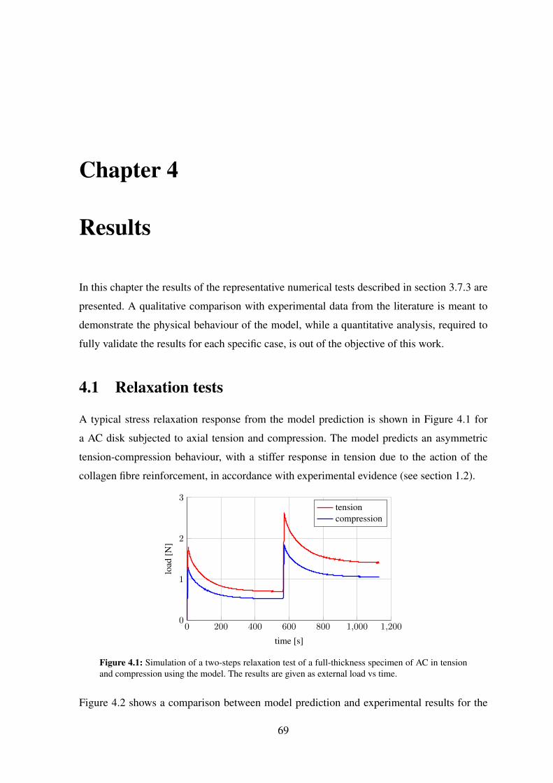
Chapter 4
Results
In this chapter the results of the representative numerical tests described in section 3.7.3 are
presented. A qualitative comparison with experimental data from the literature is meant to
demonstrate the physical behaviour of the model, while a quantitative analysis, required to
fully validate the results for each specific case, is out of the objective of this work.
4.1 Relaxation tests
A typical stress relaxation response from the model prediction is shown in Figure 4.1 for
a AC disk subjected to axial tension and compression. The model predicts an asymmetric
tension-compression behaviour, with a stiffer response in tension due to the action of the
collagen fibre reinforcement, in accordance with experimental evidence (see section 1.2).
0 200 400 600 800 1,000 1,2000
1
2
3
time [s]
load
[N]
tensioncompression
Figure 4.1: Simulation of a two-steps relaxation test of a full-thickness specimen of AC in tensionand compression using the model. The results are given as external load vs time.
Figure 4.2 shows a comparison between model prediction and experimental results for the
69
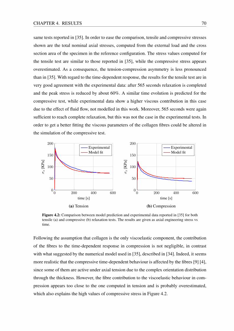
CHAPTER 4. RESULTS 70
same tests reported in [35]. In order to ease the comparison, tensile and compressive stresses
shown are the total nominal axial stresses, computed from the external load and the cross
section area of the specimen in the reference configuration. The stress values computed for
the tensile test are similar to those reported in [35], while the compressive stress appears
overestimated. As a consequence, the tension-compression asymmetry is less pronounced
than in [35]. With regard to the time-dependent response, the results for the tensile test are in
very good agreement with the experimental data: after 565 seconds relaxation is completed
and the peak stress is reduced by about 60%. A similar time evolution is predicted for the
compressive test, while experimental data show a higher viscous contribution in this case
due to the effect of fluid flow, not modelled in this work. Moreover, 565 seconds were again
sufficient to reach complete relaxation, but this was not the case in the experimental tests. In
order to get a better fitting the viscous parameters of the collagen fibres could be altered in
the simulation of the compressive test.
0 200 400 6000
50
100
150
200
time [s]
σz
[KPa
]
ExperimentalModel fit
(a) Tension
0 200 400 6000
50
100
150
200
time [s]
σz
[KPa
]
ExperimentalModel fit
(b) Compression
Figure 4.2: Comparison between model prediction and experimental data reported in [35] for bothtensile (a) and compressive (b) relaxation tests. The results are given as axial engineering stress vstime.
Following the assumption that collagen is the only viscoelastic component, the contribution
of the fibres to the time-dependent response in compression is not negligible, in contrast
with what suggested by the numerical model used in [35], described in [34]. Indeed, it seems
more realistic that the compressive time-dependent behaviour is affected by the fibres [9] [4],
since some of them are active under axial tension due to the complex orientation distribution
through the thickness. However, the fibre contribution to the viscoelastic behaviour in com-
pression appears too close to the one computed in tension and is probably overestimated,
which also explains the high values of compressive stress in Figure 4.2.
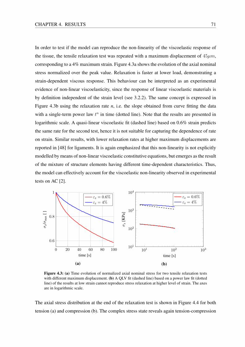
CHAPTER 4. RESULTS 71
In order to test if the model can reproduce the non-linearity of the viscoelastic response of
the tissue, the tensile relaxation test was repeated with a maximum displacement of 45µm,
corresponding to a 4% maximum strain. Figure 4.3a shows the evolution of the axial nominal
stress normalized over the peak value. Relaxation is faster at lower load, demonstrating a
strain-dependent viscous response. This behaviour can be interpreted as an experimental
evidence of non-linear viscoelasticity, since the response of linear viscoelastic materials is
by definition independent of the strain level (see 3.2.2). The same concept is expressed in
Figure 4.3b using the relaxation rate n, i.e. the slope obtained from curve fitting the data
with a single-term power law tn in time (dotted line). Note that the results are presented in
logarithmic scale. A quasi-linear viscoelastic fit (dashed line) based on 0.6% strain predicts
the same rate for the second test, hence it is not suitable for capturing the dependence of rate
on strain. Similar results, with lower relaxation rates at higher maximum displacements are
reported in [48] for ligaments. It is again emphasized that this non-linearity is not explicitly
modelled by means of non-linear viscoelastic constitutive equations, but emerges as the result
of the mixture of structure elements having different time-dependent characteristics. Thus,
the model can effectively account for the viscoelastic non-linearity observed in experimental
tests on AC [2].
0 20 40 60 80 100
0.6
0.8
1
time [s]
σz/σ
max
[]
εz = 0.6%
εz = 4%
(a)
101 102 103101
102
103
104
time [s]
σz
[KPa
]
εz = 0.6%
εz = 4%
(b)
Figure 4.3: (a) Time evolution of normalized axial nominal stress for two tensile relaxation testswith different maximum displacement. (b) A QLV fit (dashed line) based on a power law fit (dottedline) of the results at low strain cannot reproduce stress relaxation at higher level of strain. The axesare in logarithmic scale.
The axial stress distribution at the end of the relaxation test is shown in Figure 4.4 for both
tension (a) and compression (b). The complex stress state reveals again tension-compression
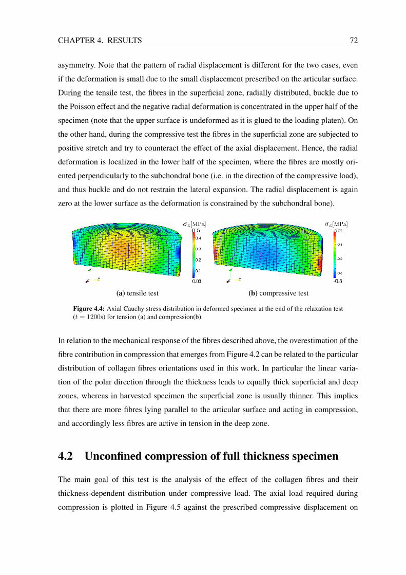
CHAPTER 4. RESULTS 72
asymmetry. Note that the pattern of radial displacement is different for the two cases, even
if the deformation is small due to the small displacement prescribed on the articular surface.
During the tensile test, the fibres in the superficial zone, radially distributed, buckle due to
the Poisson effect and the negative radial deformation is concentrated in the upper half of the
specimen (note that the upper surface is undeformed as it is glued to the loading platen). On
the other hand, during the compressive test the fibres in the superficial zone are subjected to
positive stretch and try to counteract the effect of the axial displacement. Hence, the radial
deformation is localized in the lower half of the specimen, where the fibres are mostly ori-
ented perpendicularly to the subchondral bone (i.e. in the direction of the compressive load),
and thus buckle and do not restrain the lateral expansion. The radial displacement is again
zero at the lower surface as the deformation is constrained by the subchondral bone).
(a) tensile test (b) compressive test
Figure 4.4: Axial Cauchy stress distribution in deformed specimen at the end of the relaxation test(t = 1200s) for tension (a) and compression(b).
In relation to the mechanical response of the fibres described above, the overestimation of the
fibre contribution in compression that emerges from Figure 4.2 can be related to the particular
distribution of collagen fibres orientations used in this work. In particular the linear varia-
tion of the polar direction through the thickness leads to equally thick superficial and deep
zones, whereas in harvested specimen the superficial zone is usually thinner. This implies
that there are more fibres lying parallel to the articular surface and acting in compression,
and accordingly less fibres are active in tension in the deep zone.
4.2 Unconfined compression of full thickness specimen
The main goal of this test is the analysis of the effect of the collagen fibres and their
thickness-dependent distribution under compressive load. The axial load required during
compression is plotted in Figure 4.5 against the prescribed compressive displacement on
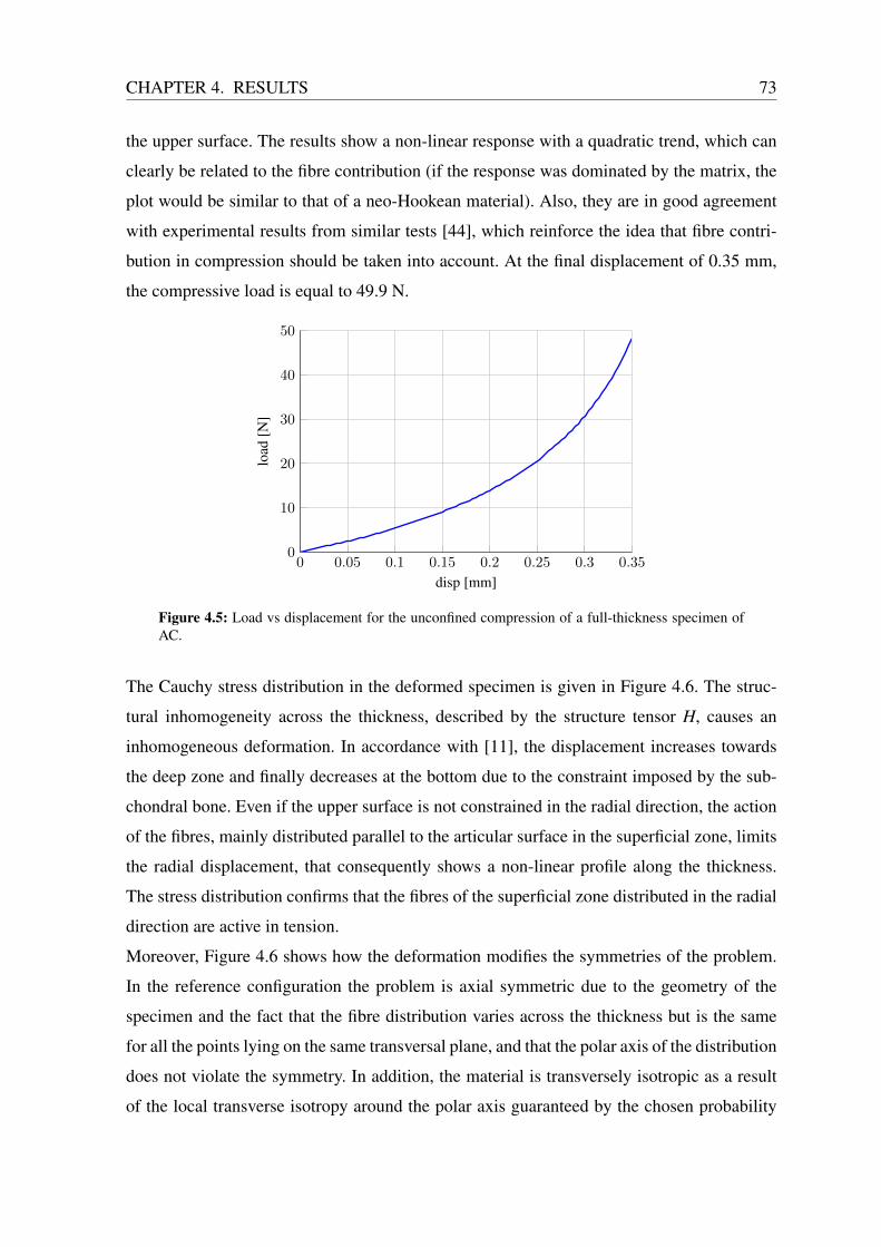
CHAPTER 4. RESULTS 73
the upper surface. The results show a non-linear response with a quadratic trend, which can
clearly be related to the fibre contribution (if the response was dominated by the matrix, the
plot would be similar to that of a neo-Hookean material). Also, they are in good agreement
with experimental results from similar tests [44], which reinforce the idea that fibre contri-
bution in compression should be taken into account. At the final displacement of 0.35 mm,
the compressive load is equal to 49.9 N.
0 0.05 0.1 0.15 0.2 0.25 0.3 0.350
10
20
30
40
50
disp [mm]
load
[N]
Figure 4.5: Load vs displacement for the unconfined compression of a full-thickness specimen ofAC.
The Cauchy stress distribution in the deformed specimen is given in Figure 4.6. The struc-
tural inhomogeneity across the thickness, described by the structure tensor H, causes an
inhomogeneous deformation. In accordance with [11], the displacement increases towards
the deep zone and finally decreases at the bottom due to the constraint imposed by the sub-
chondral bone. Even if the upper surface is not constrained in the radial direction, the action
of the fibres, mainly distributed parallel to the articular surface in the superficial zone, limits
the radial displacement, that consequently shows a non-linear profile along the thickness.
The stress distribution confirms that the fibres of the superficial zone distributed in the radial
direction are active in tension.
Moreover, Figure 4.6 shows how the deformation modifies the symmetries of the problem.
In the reference configuration the problem is axial symmetric due to the geometry of the
specimen and the fact that the fibre distribution varies across the thickness but is the same
for all the points lying on the same transversal plane, and that the polar axis of the distribution
does not violate the symmetry. In addition, the material is transversely isotropic as a result
of the local transverse isotropy around the polar axis guaranteed by the chosen probability
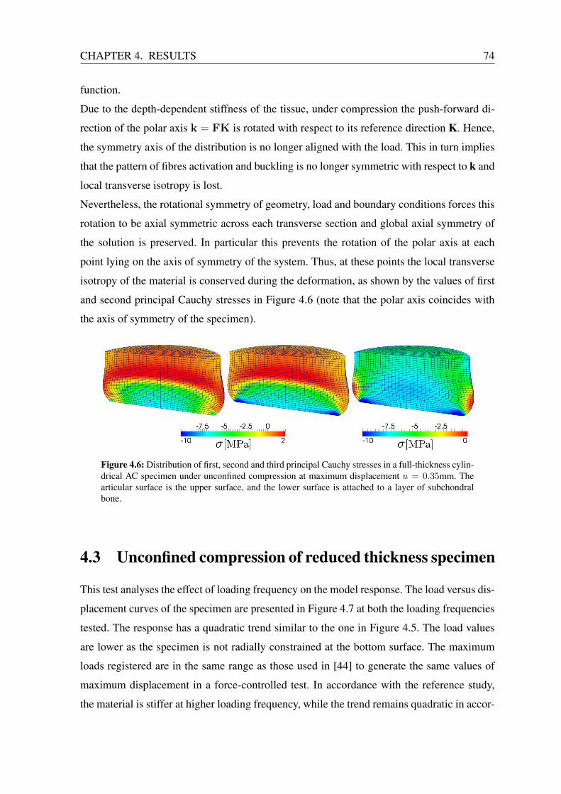
CHAPTER 4. RESULTS 74
function.
Due to the depth-dependent stiffness of the tissue, under compression the push-forward di-
rection of the polar axis k = FK is rotated with respect to its reference direction K. Hence,
the symmetry axis of the distribution is no longer aligned with the load. This in turn implies
that the pattern of fibres activation and buckling is no longer symmetric with respect to k and
local transverse isotropy is lost.
Nevertheless, the rotational symmetry of geometry, load and boundary conditions forces this
rotation to be axial symmetric across each transverse section and global axial symmetry of
the solution is preserved. In particular this prevents the rotation of the polar axis at each
point lying on the axis of symmetry of the system. Thus, at these points the local transverse
isotropy of the material is conserved during the deformation, as shown by the values of first
and second principal Cauchy stresses in Figure 4.6 (note that the polar axis coincides with
the axis of symmetry of the specimen).
Figure 4.6: Distribution of first, second and third principal Cauchy stresses in a full-thickness cylin-drical AC specimen under unconfined compression at maximum displacement u = 0.35mm. Thearticular surface is the upper surface, and the lower surface is attached to a layer of subchondralbone.
4.3 Unconfined compression of reduced thickness specimen
This test analyses the effect of loading frequency on the model response. The load versus dis-
placement curves of the specimen are presented in Figure 4.7 at both the loading frequencies
tested. The response has a quadratic trend similar to the one in Figure 4.5. The load values
are lower as the specimen is not radially constrained at the bottom surface. The maximum
loads registered are in the same range as those used in [44] to generate the same values of
maximum displacement in a force-controlled test. In accordance with the reference study,
the material is stiffer at higher loading frequency, while the trend remains quadratic in accor-
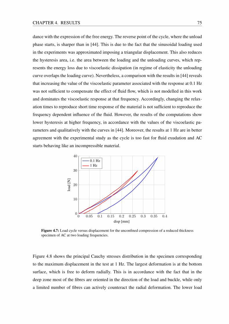
CHAPTER 4. RESULTS 75
dance with the expression of the free energy. The reverse point of the cycle, where the unload
phase starts, is sharper than in [44]. This is due to the fact that the sinusoidal loading used
in the experiments was approximated imposing a triangular displacement. This also reduces
the hysteresis area, i.e. the area between the loading and the unloading curves, which rep-
resents the energy loss due to viscoelastic dissipation (in regime of elasticity the unloading
curve overlaps the loading curve). Nevertheless, a comparison with the results in [44] reveals
that increasing the value of the viscoelastic parameter associated with the response at 0.1 Hz
was not sufficient to compensate the effect of fluid flow, which is not modelled in this work
and dominates the viscoelastic response at that frequency. Accordingly, changing the relax-
ation times to reproduce short time response of the material is not sufficient to reproduce the
frequency dependent influence of the fluid. However, the results of the computations show
lower hysteresis at higher frequency, in accordance with the values of the viscoelastic pa-
rameters and qualitatively with the curves in [44]. Moreover, the results at 1 Hz are in better
agreement with the experimental study as the cycle is too fast for fluid exudation and AC
starts behaving like an incompressible material.
0 0.05 0.1 0.15 0.2 0.25 0.3 0.35 0.40
10
20
30
40
disp [mm]
load
[N]
0.1 Hz1 Hz
Figure 4.7: Load cycle versus displacement for the unconfined compression of a reduced thicknessspecimen of AC at two loading frequencies.
Figure 4.8 shows the principal Cauchy stresses distribution in the specimen corresponding
to the maximum displacement in the test at 1 Hz. The largest deformation is at the bottom
surface, which is free to deform radially. This is in accordance with the fact that in the
deep zone most of the fibres are oriented in the direction of the load and buckle, while only
a limited number of fibres can actively counteract the radial deformation. The lower load
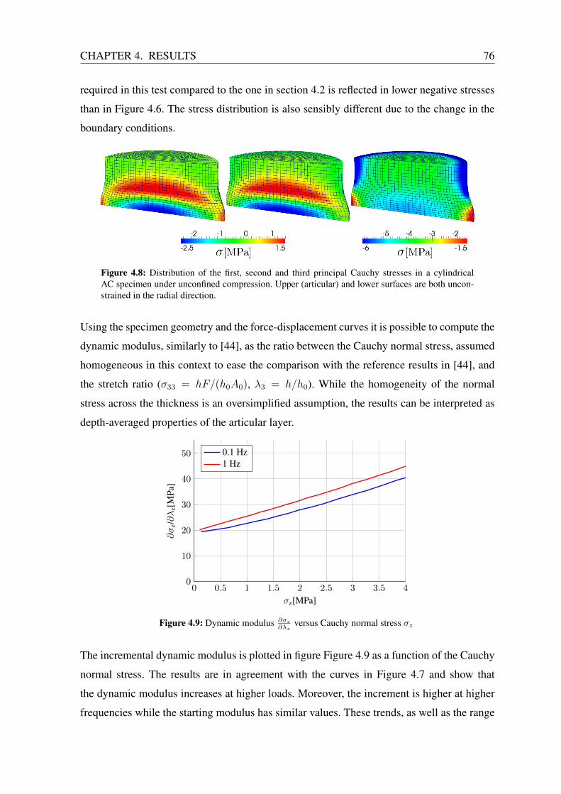
CHAPTER 4. RESULTS 76
required in this test compared to the one in section 4.2 is reflected in lower negative stresses
than in Figure 4.6. The stress distribution is also sensibly different due to the change in the
boundary conditions.
Figure 4.8: Distribution of the first, second and third principal Cauchy stresses in a cylindricalAC specimen under unconfined compression. Upper (articular) and lower surfaces are both uncon-strained in the radial direction.
Using the specimen geometry and the force-displacement curves it is possible to compute the
dynamic modulus, similarly to [44], as the ratio between the Cauchy normal stress, assumed
homogeneous in this context to ease the comparison with the reference results in [44], and
the stretch ratio (σ33 = hF/(h0A0), λ3 = h/h0). While the homogeneity of the normal
stress across the thickness is an oversimplified assumption, the results can be interpreted as
depth-averaged properties of the articular layer.
0 0.5 1 1.5 2 2.5 3 3.5 40
10
20
30
40
50
σz[MPa]
∂σ
z/∂λ
z[M
Pa]
0.1 Hz1 Hz
Figure 4.9: Dynamic modulus ∂σz
∂λzversus Cauchy normal stress σz
The incremental dynamic modulus is plotted in figure Figure 4.9 as a function of the Cauchy
normal stress. The results are in agreement with the curves in Figure 4.7 and show that
the dynamic modulus increases at higher loads. Moreover, the increment is higher at higher
frequencies while the starting modulus has similar values. These trends, as well as the range

CHAPTER 4. RESULTS 77
of computed values, are in good agreement with [44]. Moreover, the results support the
hypothesis that the non-linear stiffening of collagen fibrils in tension regulates the dynamic
properties in compression [55] through the mechanism described in the previous example.
Chapter 5
Conclusions
The present work developed a non-linear anisotropic viscoelastic constitutive model for AC,
whose characteristics were illustrated by mean of three representative numerical examples.
The first objective was to define a structural quantity that represents the distributed collagen
fibres in a continuum sense and that accounts for their directional characteristics. This was
achieved through the computation of the directional average of the structure tensor at each
material point. The use of averaging integrals it is not affected by the limitations of a finite
number of fibres and on the computational side it does not require to store the information
related to the fibre directions, but only the parameters of the distribution that represent them.
The proposed definition for the structural contribution of compressed fibres effectively ac-
counts for their distribution without influencing the value of the potential, according to the
assumption that only stretched fibres can bear load. To the author’s knowledge, such contri-
bution represents an element of innovation in the study of biological tissues with statistical
fibre orientation.
The generalized structure tensor introduced in this work extends the range of applicability
of the averaged structure tensor presented in [13] to the modelling of tissues with inhomoge-
neous mechanical properties and fibre reinforcements without a preferential direction. The
downside is represented by an increased computational cost of the model: the amount and
direction of fibres that contributes to the structure tensor must be determined at each loading
step, which in turn implies that the averaging integration has to be repeated for each material
point. The increased level of complexity is anyway necessary to model AC, while it could be
required in other applications to get more accurate predictions.
It should be noted that the developed structure representation does not account either for
78
CHAPTER 5. CONCLUSIONS 79
shear interactions between matrix and fibres or fibre-fibre interaction due to entanglement,
which can occur when fibre orientation has a statistical distribution. Such contributions are
often disregarded and they would require the definition of additional generalized invariants
to be included in the elastic potential.
The proposed approach is very general: it is compatible with any expression of the elastic
potential that accounts for the presence of a structure tensor as well as any fibre distribution
function, either in an analytical form as a probability density function or in a tabular form
from experimental data. Hence, this work provides the framework for the development of
more complex constitutive models. Moreover, AC represents only one of the possible ap-
plications of the model, which could be applied also to other tissues with statistical fibre
orientation (e.g. the adventitial layer of the arterial walls).
The results of the numerical test show that the model can effectively account for the role of
the fibre reinforcement in the response of AC. It reproduces the inhomogeneous and depth-
dependent mechanical properties of the tissue and it accounts for the contribution of collagen
under compressive load, suggesting that it should not be neglected. The computed deforma-
tion pattern is in agreement with theoretical predictions and experimental results from the
literature.
The second objective was to introduce a formulation of the intrinsic viscoelastic properties
of AC. A quasi-linear viscoelastic relation was chosen for collagen fibres, while the rest of
the solid phase was assumed to be elastic. This is a partial limitation as other constituents
(e.g. proteoglycans) are known to be viscoelastic. However, they play only a secondary role
in the intrinsic time-dependent response.
The results of the numerical tests show that the model can effectively reproduce the response
of AC observed in tension. On the other hand, the attempt to reproduce the viscoelastic
behaviour in compression did not provide acceptable results, suggesting a dominant role of
fluid-related viscoelastic response.
Nevertheless, the results demonstrate the expected frequency-related response, indicating
that the model can be tuned using the viscoelastic parameters to reproduced specific experi-
mental tests. In addition, the relaxation function was found to be strain-dependent, indicating
that the model can reproduce the non-linear viscoelastic nature of the solid phase of AC.
The last goal was to develop a suitable numerical implementation for the model. The expres-

CHAPTER 5. CONCLUSIONS 80
sion of the structure tensor in the spatial configuration was derived as well as those of the
Cauchy stress and the elasticity tensor. These quantities where included into a finite element
implementation based on efficient numerical schemes from the literature. In particular the
evolution equations where integrated according to [21], while the directional average of the
structure tensor is computed using a spherical design as in [9].
On the other hand, the dependence of the structure tensor on the deformation was disre-
garded in the derivation of the elasticity tensor as the value of the stretch in each direction
(that discriminates between the two definitions for the contribution to the structure tensor) is
taken from the previous solution step. This requires the definition of a high number of history
variables to store the stretch values, which slows the calculation of the solution and can be
a limitation for the maximum size of the problem, especially on regular personal computers.
Moreover, a decrease in the rate of convergence of the solution scheme was experienced for
relatively high compressive load. This can be related to instabilities generated by the pro-
gressive buckling of the fibres in compression, as the problem does not arise in tension.
It should also be noted that the particular choice of the strain energy potential is not based on
experimental data. However, the quadratic function used in this work accounts for the non-
linearity in the stress-strain curve due to fibre engagement and it is reported in the literature
that a second order function can be sufficient to describe cases of interest such as immature
or engineered cartilage. Moreover, it is again emphasized that the generality of the model
allows the use of a function of higher order or of a different class (e.g. exponential) without
the need to modify the implementation of the generalized structure tensor.
Similarly, the proposed fibre distribution density function is not based on experimental data
but can qualitatively reproduce the depth-dependent arrangement of collagen reported in the
literature. A drawback of the chosen distribution, which is based on a dispersion parameter
that varies linearly through the thickness, is that it defines equally thick superficial and deep
zones, whereas histological data indicate that the former should be thinner than the latter.
This is reflected in an overestimation of the fibre contribution in the superficial layer to the
compressive modulus of the tissue.
The last two remarks imply that a direct, quantitative comparison of the results of the model
with published experimental results is not possible. However, the developed constitutive
model for the solid phase of AC demonstrates correct physical behaviour and produces re-

CHAPTER 5. CONCLUSIONS 81
sults qualitatively in agreement with the literature. In particular, it is capable of predicting the
response of the tissue under tensile load both in terms of local stress and deformation and in
terms of viscoelastic behaviour. The model is also able to account for the fibre contribution in
compression, but at the current state it is not suitable for the analysis of the time-dependent
response of AC in such configuration due to the important role of fluid flow, not included in
the model.
Further enhancements include the use of experimental data for the definition of the expres-
sions for the potential and the fibre distribution, as well as for the choice of the viscoelastic
parameter. On the numerical side, the derivation of a consistent linearisation that accounts for
the dependence of the structure tensor on the deformation would improve the performance
of the model. Finally and most importantly, a formulation of the poroelastic phenomena aris-
ing from the presence of interstitial fluid should be added to the model in order to make it
suitable to describe the time-dependent response of AC in compression.
References
[1] A. Agianniotis, R. Rezakhaniha, and N. Stergiopulos. A structural constitutive model
considering angular dispersion and waviness of collagen fibres of rabbit facial veins.
BioMedical Engineering OnLine, 10:18, 2011.
[2] G.A. Ateshian and S. Park. Dynamic response of immature bovine articular cartilage in
tension and compression, and nonlinear viscoelastic modeling of the tensile response.
ASME Journal of biomechanical engineering, 128:623–630, 2006.
[3] G.A. Ateshian, V. Raja, N.O. Chahine, C.E. Canal, and C.T. Hung. Modeling the ma-
trix of articular cartilage using a continuous fiber angular distribution predicts many
observed phenomena. ASME Journal of Biomechanical Engineering, 131:061003–10,
2009.
[4] D.L. Bader, G.E. Kempson, J. Egan, W. Gilbey, and A.J. Barrett. The effects of selective
matrix degradation on the short-term compressive properties of adult human articular
cartilage. Biochimica et Biophysica Acta, 1116(2):147–154, 1992.
[5] S. Below, S.P. Arnoczky, J. Dodds, C. Kooima, and N.J. Walter. The split-line pattern
of the distal femur: a consideration in the orientation of autologous cartilage grafts.
Journal of Arthroscopic and Related Surgery, 18:613–617, 2002.
[6] F. Brezzi and M. Fortin. Mixed and hybrid Finite Element Methods. Springer-Verlag,
1991.
[7] J. Buckwalter, H. Mankin, and A. Grodzinsky. Articular cartilage and osteoarthritis.
AAOS Instructional Course Lectures, 54:465–480, 2005.
[8] Y. Cheng, J. Hootman, L. Murphy, G. Langmaid, and C. Helmick. Prevalence of doctor-
diagnosed arthritis and arthritis-attributable activity limitation. CDC: Morbidity and
Mortality Weekly Report, 59(39):1261–1265, 2010.
82
REFERENCES 83
[9] S. Federico and T.C. Gasser. Nonlinear elasticity of biological tissues with statistical
fibre orientation. Journal of the Royal Society Interface, 7(47):955–966, 2010.
[10] N. I. Fisher, T. L. Lewis, and B. J. J. Embleton. Statistical analysis of spherical data.
Cambridge: Cambridge University Press, 1987.
[11] M. Fortin, M. D. Buschmann, M. J. Bertrand, F.S. Foster, and J. Ophir. Dynamic mea-
surement of internal solid displacement in articular cartilage. Journal of Biomechanics,
29:340–360, 2003.
[12] Y.C. Fung. Biorheology of soft tissues. Biorheology, 10:139–155, 1973.
[13] T. Gasser, R.W. Ogden, and G.A. Holzapfel. Hyperelastic modelling of arterial layers
with distributed collagen fibre orientations. Journal of the Royal Society Interface,
3(6):15–35, 2006.
[14] T.C. Gasser and C. Forsell. The numerical implementation of invariant-based viscoelas-
tic formulations at finite strains. an anisotropic model for the passive myocardium.
Computer Methods in Applied Mechanics and Engineering, 200(49):3637–3645, 2011.
[15] T.C. Gasser and G. Martufi. A constitutive model for vascular tissue that integrates
fibril, fiber and continuum levels with application to the isotropic and passive properties
of the infrarenal aorta. Journal of Biomechanics, 44:2544–2550, 2011.
[16] A. Getgood, T. Bhullar, and N. Rushton. Current concepts in articular cartilage repair.
Orthopaedics and Trauma, 23:189–200, 2009.
[17] R. H. Hardin and N. J. A. Sloane. Mclaren’s improved snub cube and other new spheri-
cal designs in three dimensions. Discrete Computational Geometry, 15:429–441, 1996.
[18] W. Hayes and L. Mockros. Viscoelastic properties of human articular cartilage. Journal
of Applied Physiology, 31(4):562–568, 1971.
[19] J. Helfenstein, M. Jabareen, E. Mazza, and Govindjee S. On non-physical response in
models for fiber-reinforced hyperelastic materials. International Journal of Solids and
Structures, 47:2056–2061, 2010.
[20] G. Holzapfel. On large strain viscoelasticity: Continuum formulation and finite element
applications to elastomeric structures. Intenational Journal of Numerical Methods in
Engineering, 39:3903–3926, 1996.

REFERENCES 84
[21] G. A. Holzapfel and T. C. Gasser. A viscoelastic model for fiber-reinforced composites
at finite strains: continuum basis, computional aspects and applications. Computater
Methods in Applied Mechanics and Engineering, 190:4397–4403, 2001.
[22] G. A. Holzapfel, T. C. Gasser, and R. W. Ogden. A new constitutive framework for ar-
terial wall mechanics and a comparative study of material models. Journal of Elasticity,
61:1–48, 2000.
[23] G. A. Holzapfel, T. C. Gasser, and M. Stadler. A structural model for the viscoelastic
behavior of arterial walls: continuum formulation and finite element analysis. European
Journal of Mechanics A/Solids, 21:441–463, 2002.
[24] G. A. Holzapfel and H. W. Weizsäcker. Biomechanical behavior of the arterial wall
and its numerical characterization. Computational biology and medicine, 28:377–392,
1998.
[25] G.A. Holzapfel. Nonlinear Solid Mechanics: A Continuum Approach for Engineering.
Wiley, 2000.
[26] C. Huang, V.C. Mow, and G.A. Ateshian. The role of flow-independent viscoelasticity
in the biphasic tensile and compressive responses of articular cartilage. ASME Journal
of Biomechanical Engineering, 123:410–417, 2001.
[27] C.Y. Huang, M.A. Soltz, M. Kopacz, V.C. Mow, and G.A. Ateshian. Experimental ver-
ification of the roles of intrinsic matrix viscoelasticity and tension-compression nonlin-
earity in the biphasic response of cartilage. ASME Journal of Biomechanical Engineer-
ing, 125:84–93, 2003.
[28] U. Hueck, B. Reddy, and Wriggers P. On the stabilization of the rectangular fournode
quadrilateral element. Communications in Applied Numerical Methods, 10:555–563,
1994.
[29] J. D. Humphrey. Continuum biomechanics of soft biological tissues. Proceedings of
the Royal Society A, 459:1–44, 2003.
[30] E. B. Hunziker. Articular cartilage repair: basic science ad clinical progress. a review
of the current status and prospects. Osteoarthritis and Cartilage, 10:432–463, 2002.
REFERENCES 85
[31] S. M. Klisch. A bimodular polyconvex anisotropic strain energy function for articular
cartilage. ASME Journal of Biomechanical Engineering, 129:250–258, 2007.
[32] S.M. Klisch, R.L. Sah, P. Vena, A. Asanbaeva, and G.C. Thomas. A nonlinear con-
stituent based viscoelastic model for articular cartilage and analysis of tissue remodel-
ing due to altered glycosaminoglycan-collagen interactions. ASME Journal of Biome-
chanical Engineering, 131:101002, 2009.
[33] Y. Lanir. Constitutive equations for fibrous connective tissues. Journal of Biomechan-
ics, 16:1–12, 1983.
[34] L.P. Li and W. Herzog. The role of viscoelasticity of collagen ffiber in articula cartilage:
Theory and numerical formulation. Biorheology, 41:181–194, 2004.
[35] L.P. Li, W. Herzog, R.K. Korhonen, and J.S. Jurvelin. The role of viscoelasticity of
collagen ffiber in articular cartilage: axial tension versus compression. Medical Engi-
neering & Physics, 27:51–57, 2005.
[36] M. Lilledahl, D. Pierce, T. Ricken, G. Holzapfel, and C. de Lange Davies. Structural
analysis of articular cartilage using multiphoton microscopy: input for biomechanical
modeling. IEEE Transactions on Medical Imaging, 30(9):1635–1648, 2011.
[37] F. Maceri, M. Marino, and G. Vairo. A unified multiscale mechanical model for soft
collagenous tissues with regular fiber arrangement. Journal of Biomechanics, 43:355–
363, 2010.
[38] J.M. Mansour. Kinesiology: the mechanics and pathomechanics of human movement,
chapter Biomechanics of cartilage. Lippincott Williams & Wilkins, 2004.
[39] C. Miehe. Multisurface thermoplasticity for single crystals at large strains in terms of
eulerian vector updates. International Journal of Solids and Structures, 33:3103–3130,
1996.
[40] R.J. Minns and F.S. Steven. The collagen fiber organization in human articular carti-
lage. Journal of Anatomy, 123(2):437–457, 1977.
[41] J. Mollenhauer, M. Aurich, C. Muehleman, G. Khelashvilli, and T.C. Irving. X-ray
diffraction of the molecular substructure of human articular cartilage. Connective Tis-
sue Research, 44:201–207, 2003.
REFERENCES 86
[42] V. C. Mow, A. Ratcliffe, and A.R. Poole. Cartilage and diarthrodial joints as paradigms
for hierarchical materials and structures. Biomaterials, 13:67 – 97, 1992.
[43] S. Park and G. A. Ateshian. Dynamic response of immature bovine articular cartilage in
tension and compression, and nonlinear viscoelastic modeling of the tensile response.
ASME Journal of Biomechanical Engineering, 128(4):623–630, 2006.
[44] S. Park, C. Hung, and G. A. Ateshian. Mechanical response of bovine articular car-
tilage under dynamic unconfined compression loading at physiological stress levels.
Osteoarthritis and Cartilage, 12:65–73, 2004.
[45] D. Pierce, W. Trobin, J. Raya, S. Trattnig, H. Bischof, C. Glaser, and G. Holzapfel.
Dt-mri based computation of collagen fiber deformation in human articular cartilage: a
feasibility study. Annals of Biomedical Engineering, pages 2447–2463, 2010.
[46] D. Pierce, W. Trobin, S. Trattnig, H. Bischf, and G. Holzapfel. A phenomenological
approach toward patient-specific computational modeling of articular cartilage includ-
ing collagen fiber tracking. Journal of Biomechanical Engineering, 131:091006–1:12,
2009.
[47] D.M. Pierce, T. Ricken, and G.A. Holzapfel. A hyperelastic biphasic fibre-reinforced
model of articular cartilage considering distributed collagen fibre orientations: contin-
uum basis, computational aspects and applications. Computer Methods in Biomechan-
ics and Biomedical Engineering, pages 1–18, 2012.
[48] P. Provenzano, R. Lakes, T. Keenan, and R.J. Vanderby. Nonlinear ligament viscoelas-
ticity. Annals of Biomedical Engineering, 29:908–914, 2001.
[49] J. Rieppo, M.M. Hyttinen, E. Halmesmaki, H. Ruotsalainen, A. Vasara, I. Kiviranta,
J.S. Jurvelin, and H.J. Helminen. Changes in spatial collagen content and collagen
network architecture in porcine articular cartilage during growth and maturation. Os-
teoarthritis and Cartilage, 17(4):448–455, 2009.
[50] M. Sacks. Incorporation of experimentally-derived fiber orientation into a structural
constitutive model for planar collagenous tissues. ASME Journal of Biomechanical
Engineering, 125:280–287, 2003.
REFERENCES 87
[51] R. Shirazi, P. Vena, R.L. Sah, and S.M. Klisch. Modeling the collagen fibril network of
biological tissues as a nonlinearly elastic material using a continuous volume fraction
distribution function. Mathematics and Mechanics of Solids, 16(7):706–715, 2011.
[52] J.C. Simo. On a fully three-dimensional finite-strain viscoelastic damage model: for-
mulation and computational aspects. Computer Methods in Applied Mechanics and
Engineering, 60:153–173, 1987.
[53] J.C. Simo, R.L. Taylor, and K.S. Pister. Variational and projection methods for the
volume constraint in finite deformation elastoplasticity. Computer Methods in Applied
Mechanics and Engineering, 51:177–208, 1985.
[54] M.A. Soltz and G.A. Ateshian. A cone wise linear elasticity model for the analysis of
tension-compression nonlinearity of articular cartilage. ASME Journal of Biomechani-
cal Engineering, 122(5):576–586, 2000.
[55] J. Soulhat, M. D. Buschmann, and Shirazi-Adl A. A fibril-network-reinforced bipha-
sic model of cartilage in unconfined compression. ASME Journal of Biomechanical
Engineering, 121:340–347, 1999.
[56] A. J. M. Spencer. Constitutive theory for strongly anisotropic solids. in continuum
theory of the mechanics of fibre-reinforced composites. CISM Courses and Lectures,
282:1–32, 1984.
[57] J. K. Suh and S. Bai. Finite element formulation of biphasic poroviscoelastic model for
articular cartilage. ASME Journal of Biomechanical Engineering, 120:195–201, 1998.
[58] J.K. Suh and M.R. Di Silvestro. Biphasic poroviscoelastic behavior of hydrated bio-
logical soft tissue. ASME Journal of Biomechanical Engineering, 66:528–535, 1999.
[59] R. L. Taylor. FEAP - a finite element analysis program, version 8.2 user manual.
Berkeley, CA: University of California at Berkeley, 2007.
[60] R.L. Taylor, K.S. Pister, and G.L. Goudreau. Thermomechanical analysis of viscoelas-
tic solids. International Journal of Numerical Methods, 2:45–59, 1970.
[61] M.C van Turnhout, M.B. Haazelager, M. A. L. Gijsen, H. Schipper, S. Kranenbarg,
and J. L. van Leeuwen. Quantitative description of collagen structure in the articular
REFERENCES 88
cartilage of the young and adult equine distal metacarpus. Animal Biology, 58:353–370,
2008.
[62] P. Vena, D. Gastaldi, and R. Contro. A constituent-based model for the nonlinear
viscoelastic behavior of ligaments. ASME Journal of Biomechanical Engineering,
128(3):449–457, 2006.
[63] T. Vos, A.D. Flaxman, M. Naghavi, and R. Lozano. Years lived with disability (ylds)
for 1160 sequelae of 289 diseases and injuries 1990–2010: a systematic analysis for the
global burden of disease study 2010. Lancet, 380 (9859):2163–96, 2012.
[64] J. A. Weiss, B. N. Maker, and S. Govindjee. Finite element implementation of in-
compressible, transversely isotropic hyperelasticity. Computater Methods in Applied
Mechanics and Engineering, 135:107–128, 1996.
[65] E. W. Weisstein. Erfi, see http://mathworld.wolfram.com/erfi.html, 2005.
[66] W. Wilson, C.C. van Donkelaar, R. van Rietbergen, and R. Huiskes. The role of com-
putational models in the search for the mechanical behavior and damage mechanisms
of articular cartilage. Medical engineering and Physics, 27:810–826, 2005.
[67] S.L.Y. Woo, B.R. Simon, S.C. Kuei, and W.H. Akeson. Quasi-linear viscoelastic prop-
erties of normal articular cartilage. ASME Journal of Biomechanical Engineering,
102:85–90, 1980.
[68] P. Wriggers. Nonlinear Finite Element Methods. Springer, 2008.
[69] O.C. Zienkiewicz and R.L. Taylor. The Finite Element Method: Basis and Fundamen-
tals. Butterworth-Heinemann, 2000.
[70] O.C. Zienkiewicz and R.L. Taylor. The Finite Element Method: Solid Mechanics, vol-
ume 2. Butterworth-Heinemann, 5 edition, 2000.