Embed Size (px)
Citation preview

POLITECNICO DI TORINO
Collegio di Ingegneria Civile
Corso di Laurea Magistrale in Ingegneria Civile
Tesi di Laurea Magistrale
Optimization of Hybrid Flat Slab at ULS
Relatori
Prof. Albert de la Fuente
Prof. Maurizio Taliano
Co-Relatore
PhD (c) Stanislav Aidarov
Studente
Luca Sutera
Luglio 2019

2
Summary
Summary of figures ................................................................................................................4
Summary of tables ..................................................................................................................7
Abstract ..................................................................................................................................8
1 Introduction .....................................................................................................................9
1.1 Scope .......................................................................................................................9
1.2 Methodology .......................................................................................................... 10
2 State of the art ............................................................................................................... 11
2.1 Fibre reinforced concrete ........................................................................................ 11
2.1.1 Fibres type ...................................................................................................... 11
2.1.2 Steel fibres ...................................................................................................... 13
2.2 Steel fibre reinforced concrete ................................................................................ 14
2.3 Residual flexural tensile strength ............................................................................ 18
2.4 Full-scale slab test .................................................................................................. 26
2.4.1 Full-scale slab test at Bissen (2004). ................................................................ 26
2.4.2 Full-scale slab test at Tallin (2007). ................................................................. 32
3 Design approach for ultimate limit state ......................................................................... 35
3.1 Plastic Analysis ...................................................................................................... 35
3.1.1 Upper and lower bound theorems .................................................................... 36
3.2 Yield Line Theory .................................................................................................. 37
3.2.1 Yield line analysis proceeds ............................................................................ 38
3.3 Application of Yield-Line Method for Elevated Slabs............................................. 42
3.3.1 Mechanism I: global failure ............................................................................. 42
3.3.2 Mechanism II: Local failure ............................................................................ 46
3.4 Flexural strength of FRC element ........................................................................... 48
3.5 The arrangement of steel reinforcement .................................................................. 50
3.5.1 Top reinforcement ........................................................................................... 50
3.5.2 Bottom reinforcement ...................................................................................... 51
3.6 Punching shear in SFRC ......................................................................................... 52
4 Parametric studies ......................................................................................................... 56
4.1 Influence of 𝑓𝑐𝑘 ..................................................................................................... 59
4.2 Influence of 𝑓𝑅3𝑘 .................................................................................................. 61
4.3 Influence of As-/As+ ............................................................................................... 64
4.4 Redistribution of moments...................................................................................... 67
5 Optimization of Hybrid Flat Slab ................................................................................... 72
5.1 Static analysis ......................................................................................................... 73

3
5.1.1 Verification at punching shear .............................................................................. 77
5.2 Parametric studies .................................................................................................. 79
5.2.1 Influence of ultimate load ................................................................................ 79
5.2.2 Influence of thickness of the flat slab ............................................................... 80
5.2.3 Influence of span number ................................................................................ 81
5.2.4 Influence of fR3m .............................................................................................. 82
5.3 Economic analysis .................................................................................................. 83
6 Conclusion .................................................................................................................... 85
6.1 Future studies ......................................................................................................... 85
References ............................................................................................................................ 86
Acknowledgements .............................................................................................................. 87

4
Summary of figures Figure 1: Cross sectional geometries of fibres [1] ................................................................. 12
Figure 2 Different fibre geometries [2] ................................................................................. 12
Figure 3: Different types of steel fibres [2] ........................................................................... 14
Figure 4: Effects of fibre on the structural behaviour [3] ....................................................... 16
Figure 5: Steel fibre reinforced concrete cracking zones [3] .................................................. 17
Figure 6: Fracture surface of steel fibre-reinforced concrete [3] ............................................ 17
Figure 7: Tensile behaviour of FRC in uniaxial stress state [3] .............................................. 19
Figure 8: Typical tensile and flexural behavior of FRC [3] ................................................... 19
Figure 9: Typical arrangement for measuring CMOD [7] ...................................................... 20
Figure 10: RILEM test specimen .......................................................................................... 20
Figure 11: Crack Mouth Opening Displacement [7] .............................................................. 21
Figure 12: An example of typical results from a bending test with a softening material
behaviour. [6] ....................................................................................................................... 22
Figure 13: Tensile behavior of steel fibre reinforced concrete with different fibre content ..... 22
Figure 14: Simplified post-crack constitutive laws; plastic-rigid behavior and linear post
cracking stress- crack opening. [6] ........................................................................................ 23
Figure 15: Layout of the test slab .......................................................................................... 27
Figure 16: Construction of the full-scale HRFA slab test in Bissen, 2004 [9] ........................ 28
Figure 17: Application of displacement transducers beneath the slab [9] ............................... 28
Figure 18: Uniformly distributed load on the HRFA full-scale forging test at Bissen, 2004.[9]
............................................................................................................................................. 29
Figure 19: Deflection under SLS in the central field [9] ........................................................ 30
Figure 20: (a) Loading frame position for corner field tests, (b) Photo of the yield lines cracking
pattern of the corner field [9] ................................................................................................ 31
Figure 21: Deformed slab after loading of an edge field [9] .................................................. 31
Figure 22: Figure (a) load-deflection curve center field (b) load-deflection curve edge field . 32
Figure 23: Diagram of lines from the break to negative bending (a) and Diagram of lines from
break to positive bending. (b). [9] ......................................................................................... 32
Figure 24: Full scale test in Tallinn with test rig and deflection gauges to measure the
deformation of the slab under the loads in the uls. [10] ......................................................... 33
Figure 25: Point load vs. deformation in the full-scale HRFA forging test in Tallinn, 2007. [10]
............................................................................................................................................. 34

5
Figure 26: Moment vs curvature ........................................................................................... 36
Figure 27: Ductile moment-rotation diagram [16] ................................................................. 38
Figure 28 Example of rules for Yield Line [11] .................................................................... 39
Figure 29 Example of collapse mechanism [12] .................................................................... 40
Figure 30 Crack patterns in elevated concrete slabs with Mechanism I - II formed in: (a) x-
direction; and (b) y-direction,[4] ........................................................................................... 42
Figure 31 Yield line patterns for two most representative panels of E-SFRC slabs in: (a) x
direction; and (b) y direction. [4] .......................................................................................... 43
Figure 32: Principle of virtual work to estimate the ultimate load-carrying capacity of interior
panel of slab submitted to uniform distributed load, [4] ........................................................ 44
Figure 33: Principle of virtual work to determine ultimate load-carrying capacity of strip of
interior panel of slab subjected to uniform distributed load and line load (parallel to yield lines).
............................................................................................................................................. 45
Figure 34: Principle of virtual work to calculate flexural strength of elevated slab submitted to
point load [4] ........................................................................................................................ 46
Figure 35: Yield line patterns for local failure, [4] ................................................................ 47
Figure 36: Simplified stress/strain relationship including the residual flexural tensile strength
of fibres [6] .......................................................................................................................... 48
Figure 37: Recommended values for β .................................................................................. 54
Figure 38: Typical basic control perimeters around loaded areas ........................................... 54
Figure 39: Proposed distribution of top of reinforcement [12] ............................................... 58
Figure 40: Cross section ....................................................................................................... 59
Figure 41: Mu – qu vs fR3k .................................................................................................. 60
Figure 42: qu vs fR3k ........................................................................................................... 61
Figure 43: Mu vs fR3k .......................................................................................................... 61
Figure 44: Graph ultimate load qu vs FR3k ............................................................................. 62
Figure 45: Graph ratio x /d vs fR3k ......................................................................................... 63
Figure 46: Graph ratio Mp- / Mp+ vs fR3k ............................................................................... 63
Figure 47: Graph ultimate load qu vs Total steel reinforcement content[kg/m3] ..................... 65
Figure 48: Graph ultimate load x /d vs Total steel reinforcement content[kg/m3] .................. 66
Figure 49: Graph ultimate load Mp- / Mp+ [-] vs Total steel reinforcement content[kg/m3] .... 66
Figure 50: Simplified moment-curvature, M-χ, diagram [16] ................................................ 67
Figure 51: Evolution of deflection moment over the supports and central span sections in terms
of load [16] ........................................................................................................................... 68

6
Figure 52: Flat slab model deployed using Sap2000 ............................................................. 69
Figure 53: Elastic Moment along the y direction obtained from SAP 2000 ........................... 70
Figure 54: Percentual moment redistribution vs fR3k.............................................................. 71
Figure 55: Total steel content vs. fR3k, for a flat slab containing the Hybrid Reinforcement
designed according to the proposed design method. .............................................................. 73
Figure 56: M-/M+ vs fR3k .................................................................................................... 74
Figure 57: x/d vs fR3k .......................................................................................................... 74
Figure 58: Total steel content vs. fR3k, for plastic and elastic analysis.................................. 76
Figure 59: Flat slab model deployed using Sap2000 ............................................................. 77
Figure 60: Total steel content vs. fR3k, for different ultimate loads ...................................... 79
Figure 61: Total steel content vs. fR3k, for different thickness of the slab ............................. 80
Figure 62: Total steel content vs. fR3k, for different span number ........................................ 81
Figure 63: Total steel content for characteristic and mean tensile strength of fibre ................ 82
Figure 64. Oscillation costs [€/m3] ........................................................................................ 83

7
Summary of tables Table 1: Physical properties of typical fibre [2]..................................................................... 13
Table 2: Constitutive models in European codes and guidelines [8] ...................................... 25
Table 3: Concrete mix components [9] ................................................................................. 27
Table 4: Concrete mix components [10] ............................................................................... 33
Table 5: Common concentrations of top reinforcement over columns when using Yield Line
Design, where E.D= edge distance is the centerline of the column to the edge of slab and L is
the length of the span. [12] ................................................................................................... 50
Table 6: Conventional reinforcing steel properties ................................................................ 57
Table 7: Concrete properties ................................................................................................. 57
Table 8: Fibre properties [15] ............................................................................................... 58
Table 9: Cases studied .......................................................................................................... 60
Table 10: Cases studied ........................................................................................................ 62
Table 11: Case studied .......................................................................................................... 65
Table 12: Cases studied ........................................................................................................ 69
Table 13: Flat slab proprieties ............................................................................................... 72
Table 14: Fibre proprieties .................................................................................................... 72
Table 15: Values of dead and live loads ................................................................................ 73
Table 16: Results obtained for case analysed ........................................................................ 75
Table 17: Verification at punching for fR3k=0 ..................................................................... 77
Table 18: Verification at punching for fR3k=30.................................................................... 78

8
Abstract
Nowadays, the use of steel fibre reinforced concrete (SFRC) is increased significantly in the
field of construction industry. New standards and guidelines accepted this material as a
structural one what, in turn, permitted to broad the area of SFRC application. Executed Steel
Fibre Reinforced Concrete Slabs (ESFRCS) in the office building of LKS in Spain, Triangle
office building in Estonia and Shopping Mall in Latvia could be the examples of the performed
SFRC elements with high structural responsibility.
In fact, the implementation of SFRC for the execution of elevated slabs has the essential
advantages in comparison with traditional solutions. Optimization of resources, reduction of
execution time, decreasing of the environmental impact could be named, beyond a doubt, as
ones of aforementioned advantages. However, it should be pointed out that steel bar
reinforcement also provides clear benefits for the surface structural elements. The placement of
rebars in the required areas due to a certain value of stresses is truly among of them (what is
impossible in the case of fibres).
Therefore, within the thesis in question, the possibility of hybrid solution (rebars + steel
fibres) for elevated slabs has been studied in detail. The Ultimate Limit State design of Hybrid
Reinforced Concrete Elevated Slabs has been carried out in accordance with relevant
guidelines. Changing the proportion of fibre and standard rebars content in the established
structure, the parametric study has been developed in order to obtain the most suitable solution
in terms of structural capacity and potential costs.

9
1 Introduction
During the last decades, the notable progress has been achieved in technology of concrete
as a construction material. Nowadays, it could be found various approaches to enhance essential
properties of concrete, such as durability, crack resistance, thermal characteristics, residual
tensile strength, fire resistance and workability, for instance. One of the most innovative method
to effect almost on all mentioned characteristics is, without any doubt, the presence of fibres in
the concrete mix.
Initially, the application of fibre reinforced concrete (FRC) was limited due to the lack of
experience and knowledge regarding this technological material. As a consequence, this type
of concrete was used only for non-structural purposes or in the elements subjected to low tensile
stresses, like FRC roads, industrial pavements and precast tunnel segments. However, the
updated codes and guidelines expanded the area of FRC usage and it has been already executed
a plenty of FRC elements with high structural responsibility and the performance of elevated
steel fibre reinforced concrete slabs could be a clear example.
The execution of aforementioned pile supported slabs drew attention throughout the
world due to the evident advantages which bring the implementation of fibres instead of
traditional reinforcement such as optimization of the recourses, time savings and reduction of
environmental impact. Also, the possibility of hybrid solutions (fibre + rebars) for the plane
FRC structural elements has been recently analyzed.
1.1 Scope
Taking into consideration the relevance of the topic, the study in question has as its main
purpose of optimizing the design of a slab at the ultimate limit state in terms of structural
strength and cost with a fibre-reinforced concrete and conventional reinforcement, by assuming
some initials design hypothesis.
10
1.2 Methodology
This thesis consists of five chapters and an introductory part. The introductory part gives a
more comprehensive background to the subjects treated in the papers.
In Chapter 2, a literature study was done on fibre reinforced concrete to gain knowledge
about the material and its behaviour, strength and properties. In this report, results from
experimental tests found in literature, on slab with varying fibre contents, were used as
reference values and their material data and properties were used as input data for the design
calculations.
Chapter 3 of the thesis focuses on the theoretical bases and hypotheses taken into account
for the structural calculation. The following topics are described: the principles and applications
of yield line theory for the calculation of moments using the plastic theory, the constitutive law
used for fibre-reinforced concrete, the assumptions concerning the positioning of the
reinforcement bars and the contribution given by steel fibres to resistance to punching shear.
In chapter 4, it is carried out some parametric studies aimed to analyse the influence of the
compressive and tensile strength of the fibre reinforced concrete on bending behaviour. The
ratio between the negative and positive area of ordinary reinforcement is analyzed in order to
verify if it affects the total amount of steel. At the end, it is studied the redistribution percentage
of elastic moment for different cases.
In chapter 5, the optimization of hybrid reinforced concrete elevated slabs ultimate limit state
design has been carried out in accordance with the guidelines. Changing the proportion of fibre
and standard rebars content in the established structure, the parametric study has been
developed in order to obtain the most suitable solution in terms of structural capacity. Finally,
it is performed an analysis of potential costs.
The major conclusions are presented in chapter 6 with suggestions for future research.

11
2 State of the art
2.1 Fibre reinforced concrete
Plain concrete is a brittle material with high compressive strength in comparison with tensile
one which is approximately ten times smaller. Therefore, the implementation of reinforcement
is required in order to improve the tensile properties of the material. The traditional solution
involves the placement of the steel reinforcing bars to increase the load carrying capacity in the
zones subjected to considerable tensile and shear stresses.
Relatively new approach lies in the enhancement of concrete tensile strength by means of
material modification which includes the addition of fibres to the concrete mix. The main
purpose of the fibres is to bear the tensile stresses once the concrete element is cracked. Besides
the tensile strength improvement, fibres could influence on other properties of concrete such as
crack resistance, durability, fire resistance, fatigue resistance, ductility, etc. Also, it should be
mentioned that the fibre could be added to the concrete mix for structural and non-structural
purposes.
Generally, we can classify as structural fibres, those which considerably increase the
breaking energy of the concrete in comparison with the plain one (in this case, their contribution
should be considered in the design of the FRC elements). Non-structural fibres, in turn, are not
to be considered in the design procedure as they are aimed to effect on certain properties which
were described above.
2.1.1 Fibres type
There are a number of different parameters that effect on the properties and behaviour of
fibre reinforced concrete, such as mechanical properties of the implemented fibres and their
geometrical shape, for instance. Each fibre type is designed for a specific purpose which could
be the improvement of tensile strength, control of drying shrinkage or the improvement of fire
resistance.
One of the most essential parameter for the fibre is its geometrical characteristics which
vary crucially depending on the specific purpose: fibres could be several millimeters of length
(microfibres) up to 80 mm (macro-fibres). The diameters also differ significantly, from a

12
fraction of a micrometer to 2 mm. Also, the shape of the fibre should be taken into consideration
due to impressive diversity of this aspect: they can be straight, wave-shaped, bow-shaped,
toothed, the surface intended, twisted or irregular, as illustrated in Figure 1. The cross-section
of fibres can be different and can have a circular, square, rectangular, triangular, elliptical and
irregular cross-section as it is presented in Figure 2. Besides, in order to improve the adherence
with the concrete, the fibres can present the shaped ends, undulations, corrugations, crushing,
hooks, etc. [1][2]
The mechanical properties of the fibres and their variety in dependence on the material could
be noted in the Table 1.
Figure 2 Different fibre geometries [2]
Figure 1: Cross sectional geometries of fibres [1]

13
From the presented in Table 1 types of fibres, steel ones are used the most in structural
purposes. Given that this thesis focuses on elevated slabs which, by default, faces the
considerable stresses, the above mentioned type of fibres is to be described in more detail.
2.1.2 Steel fibres
The steel fibres for concrete mix are discontinuous, with a discrete and uniform distribution
that gives the material a high degree of homogeneity and isotropy. Generally, the dimensions
of the steel fibres vary between 0.25 mm and 0.80 mm in diameter and the length is in the range
from 10 up to 75 mm.
The following parameters are used in the characterization of steel fibres:
• Slenderness or aspect ratio: it is defined as the relationship between the length of the
fibre and its diameter ( 𝑙𝑓
𝜙𝑓).
Table 1: Physical properties of typical fibre [2]

14
• The tensile strength: this parameter depends on the quality of the steel. For a low or
medium carbon content, the average resistance oscillates between 400 and 1500MPa,
while it could reach 2000Mpa with higher carbon content.
• Shape: It has great importance for the adherence between fibre and concrete, as shown
in chapter 2.1.1. It could be appreciated the variety of possible shapes in more detail by
means of .
The fibre length is recommended to be at least 2 times the size of the larger aggregate.
Therefore, the length of steel fibres is usually of 2.5 to 3 times of the maximum aggregate size.
In addition, the diameter of the pumping pipe requires that the length of the fibre be less than
2/3 of the diameter of the pipe. However, the length of the fibre must be sufficient to give the
necessary adhesion to the matrix and to avoid pull-outs too easily.
2.2 Steel fibre reinforced concrete
Steel fibre reinforced concrete (SFRC) is widely used in different fields of construction
industry. The properties of steel fibres allows to improve both structural and non-structural
characteristics of the material. However, it could be noted that recent studies are focused more
on the possible applications of SFRC in structural purposes due to improved characteristics of
the fibres (both mechanical and geometrical) and the appearance on new codes and guidelines
as it was stated previously. Nowadays, the presence of fibres in the concrete mix is able to
provide the partial or even total substitution of the conventional reinforcement due to high
residual tensile strength, ductility and toughness of the material in question.
Figure 3: Different types of steel fibres [2]

15
Experimental studies have shown that that normally used fibre volume in concrete does not
lead to an increased strength before cracking. [3] The major role of the steel fibre reinforcement
is to control the cracking of the concrete and give a contribution to the capacity after cracking.
The use of steel fibres is a well-acknowledged methodology to improve the tensile
performance and toughness of concrete. Beside the better structural performances resulting
from the enhanced mechanical properties, FRC allows a better shrinkage and crack control
leading to increased structure durability. Stress redistribution resulting from the high internal
redundancy of these structures may allow exploiting the post-cracking strength and toughness
of SFRC, leading to a possible reduction of conventional reinforcement. The aforementioned
partial or total substitution of conventional rebars allows reducing the construction time and
costs in comparison with traditional Reinforced Concrete (RC) structures. [4]
Therefore, advantages of SFRC slab primarily include the economic aspects, followed by
the improved strength and ductility, increased speed of construction, reduction of joints, and
shrinkage crack width control in continuous joint-free slabs. Nevertheless, it should be noted
that there is still some aspects to be covered and dynamic behavior, seismic design and long-
term behavior are among them.
Mechanical properties
Steel fibres significantly increase the ductility of the concrete and also improve the residual
tensile strength of the material. The main task of the added fibre is to bridge cracks that occur
in the matrix and transfer tensile stresses across the cracks. The fibre contributes to improved
crack control by causing large single cracks to be replaced by a system of microcracks with
considerably smaller crack widths. [1]
16
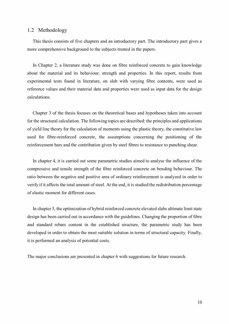
Several studies and tests carried out over the years has highlighted some important
properties, The effect of fibre in terms of crack bridging under the application of sectional forces
M, V and N, Figure 4, are listed below. [1][4][5]
- Increased shear resistance
- Increased punching resistance
- Increased dowel effect
- Inhibits growth of splitting cracks
- Increased confinement of anchored bars
- Reduced crack spacing
- Reduced crack widths
- Increased moment resistance
- Increased flexural stiffness
- Increased ductility in compression
The post-cracking behavior of concrete, however, is significantly improved due to the fibre
contribution. SFRC obtains a significant increase in the ultimate tensile strain and displays a
distinct and stable residual tensile strength after cracking, even as the crack widths increase. [1]
Factors that influence on the material properties of fibre-reinforced concrete are the
individual material properties of the matrix and the fibres, respectively, and the bond strength
between the matrix and fibres. Furthermore, the amount of fibres, the orientation and
distribution of fibres within the matrix are of importance.
Figure 4: Effects of fibre on the structural behaviour [3]

17
The fibres is generally mixed into the concrete before pumping the concrete into the
formwork, and the aim is to obtain a random fibres distribution and orientation. The distribution
and the orientation of the fibres may be prevented from distributing freely and can be influenced
by factors such as the method of placement, equipment used, such as reinforcement bars, and
properties of the fresh concrete.
The fibre contribution leads to a more ductile failure for SFRC than for plain concrete, and
the failure is mainly caused by fibre pull-out.[3] The tensile deformation capacity is improved,
resulting in an increased critical crack opening. The critical crack opening is defined as the one
where no stress can be transferred, as it is illustrated in Figure 5.
While Figure 6, shows a real fracture surface of SFRC after failure due to fibre pull-out, in
which the randomly distributed and oriented fibres are clearly displayed.
Figure 5: Steel fibre reinforced concrete cracking zones [3]
Figure 6: Fracture surface of steel fibre-reinforced concrete [3]

18
Failure of SFRC due to fibre pull-out is desirable in order to obtain ductility and toughness
during failure. Therefore, the fibre must be adequately ductile to prevent fibre fracture due to
bending. Furthermore, the bond strength between the fibre and the matrix must be of the same
magnitude, or higher, than the tensile strength of the matrix. [3]
For steel fibres with hooked ends a significant energy dissipation arises as the fibre is
straightened and plastically deformed. This dissipated energy becomes part of the fracture
energy of the concrete. The fracture energy is defined as the area under the stress-crack opening
curve in tension and is the energy required for crack propagation [1]. Consequently, SFRC
displays significantly higher fracture energy than plain concrete.
2.3 Residual flexural tensile strength
One of the most critical points in SFRC theory is to predict the tensile behavior of the
material and especially to quantify the residual stresses in tension for a cracked section. After
cracking, the SFRC displays a relatively stable residual tensile strength, even as the crack
widths increase. The residual tensile strength, 𝑓𝑅,𝑖, is defined as the residual tensile force
resultant acting on a unit area of a cracked section in the concrete. During the design procedure,
the contribution of fibres can be introduced by considering FRC as a homogeneous material
with higher toughness, represented by the residual tensile strength.
Depending on the fibre content, the concrete might have strain-softening or hardening
behaviour. A strain-softening material behavior is referred to as a behavior where the stress
reduces with continuous development of plastic strains, whereas for strain-hardening material,
the stress value increase after the crack deformation.
For deeper understanding of FRC behaviour, the uniaxial tension response of the material
in question is showed in Figure 7. For strain-softening materials a localized single crack
characterizes the tensile behavior, as seen in the tensile diagram.

19
In comparison to plain concrete, neither the tensile strength nor the modulus of elasticity of
fibre-reinforced concrete is significantly affected. The fibre mainly affects the tensile fracture
behavior and the post-cracking properties. For FRC with a low to moderate fibre content (<
1%) the stress-strain curve is characterized by a strain-softening behavior, as shown in figure
7. After the tensile strength is reached, the curve in this case decreases relatively steeply, but
whereas the curve for plain concrete continues decreasing until zero. The curve for FRC
typically increases again as the fibre starts acting by carrying tensile stresses across cracks.
The last part of the curve, having an approximately constant stress value, displays the residual
tensile strength of the FRC.
Figure 7: Tensile behaviour of FRC in uniaxial stress state [3]
Figure 8: Typical tensile and flexural behavior of FRC [3]

20
Figure 8 shows typical tensile and flexural behavior of FRC. As it could be appreciated in
the figure above that FRC can provide deflection hardening in bending despite the softening
response in uni-axial tension. Also, it could be noted that in the case of softening behavior, the
deformations localize in one crack, while the hardening one leads multiple cracking before
reaching the peak value. [3]
Measuring the flexural tensile strength
According to FIB model code [6], the strength of fibres is measured as a residual flexural
tensile strength. This can be done by performing three point bending test (3PBT). The main
principle of the test is to evaluate the behaviour of SFRC in terms of residual flexural tensile
strength values determined from the load-crack mouth displacement curve or load-deflection
curve obtained by applying a centre-point load on a simply supported notched prism. The FIB
model code proposes that it is to be done in accordance with EN 14651 (2005).[7]
The short description of the test procedure is: a simply supported beam with a span length
of 500 mm and nominal size (width and depth) of 150 mm is to be tested. In the middle of the
span, a notch is placed with a height of 25 mm and a maximum width of 5 mm, seen in Figure
9. A concentrated load is placed in the middle of the beam. The mentioned load should have
the established rate of increase and at the same time the crack mouth opening displacement
(CMOD) in the notch is to be measured. The result from the bending test of RILEM beam is
shown in Figure 10 and 11
Figure 10: RILEM test specimen
Figure 9: Typical arrangement for measuring CMOD [7]

21
Different values of the residual flexural tensile strength, 𝑓𝑅,𝑖, should be evaluated according to
the following equation
𝑓𝑅,𝑗 =3𝐹𝑗𝑙
2𝑏ℎ𝑠𝑝2 (2.1)
Where
𝑓𝑅,𝑖 is the residual flexural tensile strength corresponding to CMODi, [MPa]
𝐹𝑖 is the load corresponding to 𝐶𝑀𝑂𝐷𝑖, [kN]
𝐶𝑀𝑂𝐷𝑖 is the crack mouth opening displacement, [mm]
𝑙 is the span of the specimen, [mm]
𝑏 is the width of the specimen, [mm]
ℎ𝑠𝑝 is the distance between the notch tip and the top of the specimen, [mm]
Figure 10: RILEM bending test [3]
Figure 11: Crack Mouth Opening Displacement [7]

22
The values 𝑓𝑅1 and 𝑓𝑅3 are obtained from the corresponding 𝐶𝑀𝑂𝐷1 and 𝐶𝑀𝑂𝐷3, respectively
(Figure 12)
The fibre content effects significantly on the residual tensile strength – CMOD curve as it
possible to appreciate below:
Figure 13: Tensile behavior of steel fibre reinforced concrete with different fibre content
Figure 12: An example of typical results from a bending test with a softening material behaviour. [6]

23
Constitutive equation
The European standards and instructions which provide a constitutive equation of SFRC in
tension are, in chronological order of appearance, the following:
- German standard DBV,
- RILEM,
- Italian standard CNR-DT 204,
- Spanish instruction EHE
- IB Model Code.
Most of them propose two diagrams, one for ultimate limit state design and the other one
serviceability limit state. The proposed models could be obtained via different experimental
tests for any SFRC mix. The three point bending test is the most common one for this objective.
There are many constitutive models of the SFRC, both experimental and theoretical, and there
is no one that imposes itself on the others. One of this is proposed from FIB Model Code.
The FIB model code simplifies the real response in tension, as shown in Figure 14, into two
stress-crack opening constitutive laws, a linear post crack softening or hardening behavior, and
a plastic rigid behavior,
Figure 14 Simplified post-crack constitutive laws; plastic-rigid behavior and linear post cracking stress- crack opening. [6]

24
The parameter 𝑓𝐹𝑡𝑠 represents the serviceability residual strength, defined as the post-
cracking strenght for crack opening at SLS. On the other hand, 𝑓𝐹𝑡𝑢 represents the ultimate
residual strenght and it is associated with the ULS crack opening 𝑤𝑢, which is the maximum
crack opening accepted in the structural design and its value depends on the required ductility
and therefore should not exceed 2.5mm, according to the FIB model code.
𝑓𝐹𝑡𝑠 = 0.45𝑓𝑅1 (2.2)
𝑓𝐹𝑡𝑢 = 𝑓𝐹𝑡𝑠 −𝑤𝑢
𝐶𝑀𝑂𝐷3(𝑓𝐹𝑡𝑠 − 0.5𝑓𝑅3 + 0.2𝑓𝑅1) (2.3)
From a table produced by Ana Blanco [8] , it is possible to visualize the tensile behavior of
the SFRC for the different standards. Is should be mentioned that for the thesis in question, the
rigid-plastic constitutive law has been applied in accordance with FIB Model Code.

25
Table 2: Constitutive models in European codes and guidelines [8]

26
2.4 Full-scale slab test
As it was stated previously, the high fibre content could totally substitute the traditional
reinforcement in concrete structures. Despite the fact, that it is possible to verify the statement
above by standard design approaches using the appropriate constitutive laws (see Subchapter
2.3), the experimental test were demanded due to the lack of experience in this area.
First full-scale tests to evaluate the structural behavior during the elastic and plastic phases
of fibre-reinforced concrete were carried out in Bissen (2004) and Tallinn (2007). [9][10]
2.4.1 Full-scale slab test at Bissen (2004).
The slab was cast and tested in June 2004 and October 2004, respectively. The test
consisted of determining the resistant capacity of a 200 mm thick slab with concrete reinforced
with steel fibres. The main challenge of the experimental campaign in question was to execute
the elevated steel fibre self-compacting concrete slab (ESFRSCCS) and to subject the latter to
different types of load in order to evaluate the response of the structure. The full-scale
specimen had the overall dimensions of 18,30 x 18,30 m and a designed thickness of 20 cm.
As it is possible to appreciate in the Figure 15, the slab consisted of 9 fields and was supported
by 16 steel columns with top plates of 30 x 30 cm. Keeping in mind the Canadian Standard,
each column strip had an additional reinforcement in the lower surface to fulfil the requirement
of anti-progressive collapse reinforcement.[9]

27
In the following table 3, it is resumed the concrete mix components used in this test carried
out.
Concrete mix components Designation Unit
Characteristic cylindrical compressive
strength, fyk [MPa] 35
Cement content [kg/m3] 350
Water/cement [-] 0,5
TABIX fibre dosage [kg/m3] 100
Steel fibres length [mm] 50
Steel fibres diameter [mm] 1,3
Steel tensile strength [MPa] 900
Table 3: Concrete mix components [9]
Table 3: Concrete mix components [9]
Figure 15: Layout of the test slab

28
It is possible to notice that the fibre content was impressive even though the appropriate
workability was achieved as it possible to observe in the Figure 16
The SFRC was placed into the formwork, without any vibration, which results in a
significant reduction in execution time and, therefore, a significant cost saving.
Before the application of loads, a precise leveling was performed by using an electronic leveling
device. The leveling allows an accuracy of 0.1 mm. The slab was monitored from its lower face,
as can be seen in Figure 17, using vertical strain gauges and strain gauges to detect the onset of
cracks and the emergence of breaking lines.
Figure 16: Construction of the full-scale HRFA slab test in Bissen, 2004 [9]
Figure 17: Application of displacement transducers beneath the slab [9]

29
Initially, the flat slab was loaded with a uniformly distributed load of 1 to 6 kN/m2 using tanks
filled with water. (Figure 18).
All tanks were connected to each other by pipes. These connecting pipes allow equalization
of the water level in each tank. The loads were gradually increased by filling the ballast tanks
with water. Crack observations were carried out at load levels of p = 1.00, 2.50, 3.00, 4.50 and
6 kN/m². The radial cracks on the top surface at the supports that already existed before life
loads were applied did not increase significantly. On the lower surface, no cracks could be
found. With this evenly distributed load, elastic deformations of less than 5 mm were obtained,
which did not increase after seven days of placing the load. The load-deflection curves are
shown in the Figure 19 and they show a linear elastic behavior. Initial cracks might occur in the
real structure on top of the columns and probably in the field as well, but crack widths are much
smaller than 0.2 mm.
Figure 18: Uniformly distributed load on the HRFA full-scale forging test at Bissen, 2004.[9]

30
The last step of the testing program consisted of determining the ultimate load of the slab,
by applying a central point load until breakdown. Obtained results proved the theoretically
estimated behavior of the SFRC.[9]
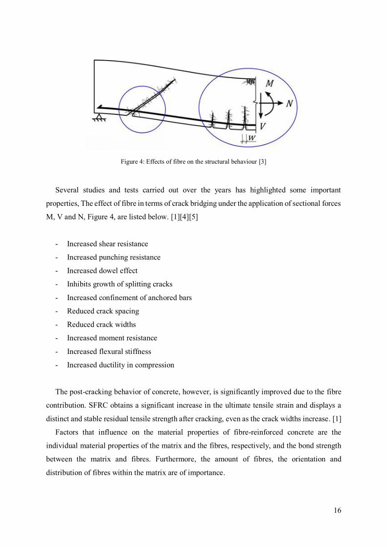
Figures 20.a and 20.b show, respectively, an image of the point load test on a corner grid
and the negative yield lines cracking pattern on the upper face of the corner field.
Figure 19: Deflection under SLS in the central field [9]
31
Figure 20: (a) Loading frame position for corner field tests, (b) Photo of the yield lines cracking pattern of the
corner field [9]
Also, is possible to show the deformation of the edge slab under an acting load. (Figure 21).
In the central field a breaking load of 450 kN was reached, and in the corner areas a breaking
load of 250 kN was reached. However, after reaching this last load, the plate still resisted a
uniformly distributed constant load of 6 kN/m2 up to a deformation of 260 mm without
collapsing.
The final tests of the load bearing capacity of center, edge and corner fields were done by
using a 700 kN hydraulic test cylinder with 200 mm stroke. The maximum load bearing capacity
of the center field was Pmax = 462.3 kN. This was equal to a uniformly distributed load of p =
25.7 kN/m², including the self-weight of the structure the load bearing capacity was 30.7 kN/m²,
if the center field is loaded only.
Figure 21: Deformed slab after loading of an edge field [9]
(a) (b)

32
The tested center, edge, and corner fields of the slab had developed a fan pattern of radial yield
lines on the lower surface and tangential yield lines on the upper surface like shown in the
Figure 23. Multiple cracking guaranteed small crack width even at loading conditions far above
service loads. The slab had performed very ductile.
2.4.2 Full-scale slab test at Tallin (2007).
Similarly to the Bissen experiment, the test carried out in Tallinn consisted of determining
the strength of the 180 mm thick slab with steel fibre reinforced concrete, without passive
reinforcement. The 5 meters span flat slab was executed and it was supported by 300x300 mm
Figure 22: Figure (a) load-deflection curve center field (b) load-deflection curve edge field
(a) (b)
(a) (b)
Figure 23: Diagram of lines from the break to negative bending (a) and Diagram of lines from break to positive bending. (b). [9]
(a) (b)

33
square plan punctual supports, forming a regular arrangement of 4 x 4 of 16 pillars. [10]
Table 4: Concrete mix components [10]
As in the Bissen test, a uniformly distributed load of 6 kN/m2 was applied, the effects of which
were deformations of less than 5 mm. Concentrated loads were also imposed on the centre slab
and also on the corner slab (Figure 24).
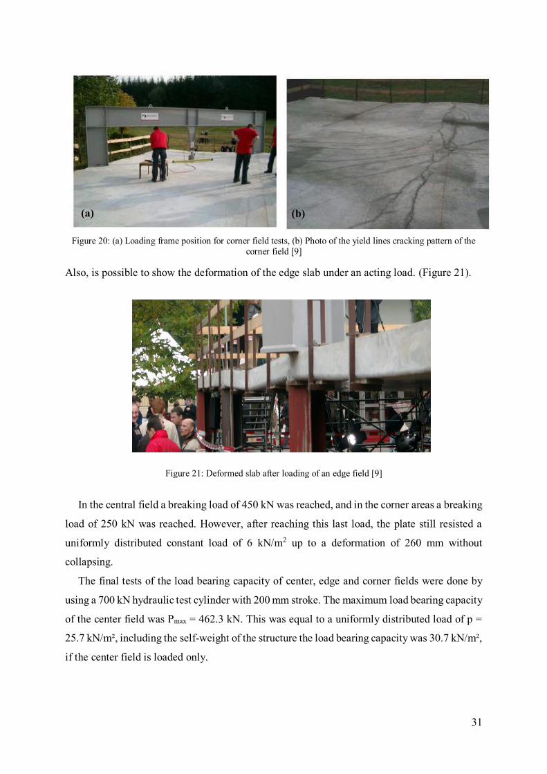
Figure 25 demonstrates the load-deformation curve obtained within the test. The point load
was increased up to a value of 340 kN and then the prototype was unloaded. The last step of
the experimental procedure was to lead the structure to a failure.
Concrete mix components
Designation Unit
Characteristic cylindrical compressive
strength, fyk [MPa] 35
Cement content [kg/m3] 350
Water/cement [-] 0,5
TABIX fibre dosage [kg/m3] 100
Steel fibres length [mm] 50
Steel fibres diameter [mm] 1,3
Steel tensile strength [MPa] 900
Figure 24: Full scale test in Tallinn with test rig and deflection gauges to measure the deformation of the slab under the loads in the uls. [10]
34
The first crack appeared with a load of 125 kN and a vertical deformation under the load of
4 mm. The maximum load reached, as it is shown in the graph above, was 600 kN which led to
an excessive cracking of the bottom surface of the slab. Load of 240 kN produced the deflection
of 10 mm and it was reached just below the point of application of the point load without
collapsing, what indicates an extremely ductile behavior of the SRFC slab, but with the
formation of hundreds of cracks from 0.1 to 0.3 mm wide. From a load of 480 kN the cracks
created increased their width to 3.5 mm.
Conclusion
Summarizing the obtained results of the described tests, it could be highlighted, that this new
type of flat slab structures had proven its feasibility. As a brief conclusion, it could be noted the
following:
• The design method involves both elastic analysis and plastic analysis to satisfy the
serviceability limit state and ultimate limit state, respectively.
• There is a substantial increase in load from the appearance of the first crack to rupture
due to the plasticity provided by the fibres and the high degree of hyperstatism of the
slab.
• To calculate the ultimate load is used the plastic theory, in this sense, the method of
yield lines proposed by Johansen is compatible.
Figure 25: Point load vs. deformation in the full-scale HRFA forging test in Tallinn, 2007. [10]

35
3 Design approach for ultimate limit state
ACI 544.6R-15 (American Concrete Institute) [4] provides the design procedure of the
elevated concrete slabs which have steel fibres as the primary reinforcement. It should be noted,
that still it is recommended to place a minimum amount of rebars, so called “anti-progressive
collapse reinforcement”. [4] However, as it was demonstrated by several research studies, fibres
represent a highly performing reinforcement for resisting diffused stresses, while localized
stresses are better resisted by rebars. This means that one can use fibre reinforcement only, but
the amount of fibres should be significantly increased in the whole structure in order to resist
high stresses acting only in small areas. Therefore, new studies are focusing on combining
fibres and rebars.
The design of SFRC structures is generally quite difficult as the non-linear tensile properties
of the composite material have to be properly included in the calculations. Referring to SFRC
slabs, the design procedures suggested by the codes are usually based on the Yield Lines
Theory.
3.1 Plastic Analysis
The design procedure based on plastic analysis is only suitable when the critical sections
have sufficient rotation capacity combined with possibility of the formation of plastic hinges,
until the mechanism of structural collapse is obtained Nevertheless, the fibres addition in the
concrete matrix provides a high-ductile behavior, leading to a proper use of the plastic theory.
The plastic analysis should be based either on the lower bound (static) or the upper bound
(kinematic) theorem, described in the chapter 3.1.1. When applying methods based on the
theory of plasticity it should be ensured that the deformation capacity of critical areas is
sufficient for the envisaged mechanism to be developed. The effects of previous applications
of loading may generally be ignored and a monotonic increase of the intensity of the actions
may be assumed.
As it is stated in the FIB model code 2010 [6], plastic analysis of beams, frames and slabs
with the kinematic theorem without any check of the rotation capacity may be used for the
ultimate limit state if all the following conditions are met:

36
- The area of tensile reinforcement is limited to such a value that at any section
o 𝑥𝑢
𝑑≤ 0.25 for concrete strength classes ≤ C50;
o 𝑥𝑢
𝑑≤ 0.15 for concrete strength classes ≥ C55;
- Reinforcing steel is either Class B or C;
- The ratio of the moments at intermediate supports to the moments in the span is between
0.5 and 2
- The ultimate moment Mu has to be always higher or equal to the moment of cracking
Mf, to avoid brittle failure and therefore ensure a plastic rotation. As shown in the
following Figure 26.
3.1.1 Upper and lower bound theorems
Plastic analysis methods derive from the general theory of structural plasticity, which states
that the collapse load of a structure lies between two limits, an upper bound and a lower bound
of the true collapse load. These limits can be found by well-established methods. A full solution
by the theory of plasticity would attempt to make the lower and upper bounds converge to a
single correct solution. The lower bound theorem and the upper bound theorem, when applied
to slabs, can be stated as follows:
• Lower bound theorem: If, for a given external load, it is possible to find a distribution
of moments that satisfies equilibrium requirements, with the moment not exceeding the
yield moment at any location, and if the boundary conditions are satisfied, then the given
load is a lower bound of the true carrying capacity.
Figure 26: Moment vs curvature
37
• Upper bound theorem: If, for a small increment of displacement, the internal work
done by the slab, assuming that the moment at every plastic hinge is equal to the yield
moment and that boundary conditions are satisfied, is equal to the external work done
by the given load for that same small increment of displacement, then that load is an
upper bound of the true carrying capacity.
If the lower bound conditions are satisfied, the slab can certainly carry the given load,
although a higher load may be carried if internal redistributions of moment occurred. If the
upper bound conditions are satisfied, a load greater than the given load will certainly cause
failure, although a lower load may produce collapse if the selected failure mechanism is
incorrect in any sense. Within the plastic analysis of structures, it should be considered either
lower bound theorem or the upper one, not both, and precautions are taken to ensure that the
predicted failure load at least closely approaches the correct value.
3.2 Yield Line Theory
One practical method for the plastic analysis of slabs is the Yield Line Theory [11]. This
theory is an analysis approach for determining the ultimate load capacity of reinforced concrete
slabs and was pioneered by K.W. Johansen in the 1940s. The yield line method of analysis for
slabs is an upper bound method, and consequently, the failure load calculated for a slab with
known flexural resistances may be higher than the true value. For this reason, the results are
either correct or theorically unsafe. It is possible to applicate this theory only for ductile (under
reinforced) slabs.
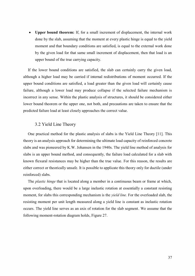
The plastic hinge that is located along a member in a continuous beam or frame at which,
upon overloading, there would be a large inelastic rotation at essentially a constant resisting
moment, for slabs this corresponding mechanism is the yield line. For the overloaded slab, the
resisting moment per unit length measured along a yield line is constant as inelastic rotation
occurs. The yield line serves as an axis of rotation for the slab segment. We assume that the
following moment-rotation diagram holds, Figure 27.

38
The advantages of Yield Line over Linear Elastic Analysis are [11]:
• Simpler to use (computer not necessary);
• Linear elastic only tells you when the first yield occurs. Y.L. gives the ultimate capacity of
the slab - what it takes to cause the collapse;
• Helps to understand ultimate behavior;
• Good for nonstandard shapes.
Disadvantages are:
• Requires experience in order to estimate the most likely failure mechanism because dangerous
designs are possible without checking.
• Does not give an idea of slab behavior in service.
3.2.1 Yield line analysis proceeds
The design procedure should be started with estimation of the yield line pattern of the
structure in question. There are strictly established rules for this task which could be found
below (Figure 28):
Figure 27: Ductile moment-rotation diagram [16]

39
• Yield lines divide the slab into rigid regions which remain plane through the collapse;
• Yield lines are straight lines because they represent the intersection of two places.
• Axes of rotation generally lie along lines of support and pass over any column;
• Yield lines between adjacent rigid regions must pass through the point of intersection
of the axes of rotation of those regions;
• Yield lines must end at a slab boundary;
• Continuous supports repel and a simple support attracts yield lines.
• Yield line forms under concentrated loads, radiating outward from the point of
application.
Figure 28 Example of rules for Yield Line [11]

40
As it was stated previously, firstly, the correct failure mechanism should be established by
means of correct position of yield lines (Figure 29)
The virtual work method is used to calculate the ultimate load for yield line analysis. In the
virtual work method, it is assumed that at failure there is no loss of energy in the slab, which
means that the internal work is equal to the external one.
𝐸𝑥𝑡𝑒𝑟𝑛𝑎𝑙 𝑤𝑜𝑟𝑘 = 𝐼𝑛𝑡𝑒𝑟𝑛𝑎𝑙 𝑤𝑜𝑟𝑘
∑(N ∙ δ)for all regions = ∑(m ∙ l ∙ θ)for all regions (3.1)
Where
𝑁 is the load(s) acting within a particular region [kN or kN/m2]
𝛿 is the vertical displacement of the load(s) N on each region expressed as a fraction of
unity [m]
𝑚 is the moment or moment of resistance of the slab per metre run represented by the
reinforcement crossing the yield line [kNm/m]
𝑙 is the length of yield line or its projected length onto the axis of rotation for that region
[m]
θ is the rotation of the region about its axis of rotation [m/m]
The external work done is the total load on the slab times the average displacement it moves
through; the internal work is the moment capacity of the yield line times the rotation it moves
through along the length.
Figure 29 Example of collapse mechanism [12]

41
Once a valid failure pattern (or mechanism) has been postulated, either the moment, m, along
the yield lines or the failure load of a slab, N (or indeed n kN/m2), can be established by applying
the above equation.
So, the Yield line analysis proceeds in this way [12]:
- Quantifying External work
The external work is calculated by taking, in turn, the resultant of each load type (i.e.
uniformly distributed load, line load or point load) acting on a region and multiplying it by its
vertical displacement measured as a proportion of the maximum deflection implicit in the
proposed yield line pattern. The total energy expended for the whole slab is the sum of the
expended energies for all the regions.
- Quantifying internal work
The internal energy dissipated is calculated by taking the projected length of each yield line
around a region onto the axis of rotation of that region, multiplying it by the moment acting on
it and by the angle of rotation attributable to that region. The total energy dissipated for the whole
slab, as for the external work, is the sum of the dissipated energies of all the regions.
- External work = Internal work
By using the equation 3.1, the value of the unknown i.e. either the moment, m, or the load,
N, can then be established. If deemed necessary, several iterations may be required to find the
maximum value of m (or the minimum value of load capacity) for each chosen failure pattern.

42
3.3 Application of Yield-Line Method for Elevated Slabs
According to ACI 544.6R-15 [4], the dominant failure mode for the flat slabs is to be
produced by the a uniformly distributed load, with crack patterns that are characterized in two
simplified mechanisms, as shown in Figure 30.
3.3.1 Mechanism I: global failure
The first collapse mechanism associated with flat slabs on a rectangular grid of columns are
showed in the Figure 31. The fracture line pattern consists of parallel positive and negative
moment lines with the negative yield line forming along the axis of rotation passing over a line
of columns. This forms a folded plate type of collapse mode with maximum deflection taken as
unity occurring along the positive yield line.
Figure 30 Crack patterns in elevated concrete slabs with Mechanism I - II formed in: (a) x-direction; and (b) y-direction,[4]

43
Applying the principle of virtual work represented in Figure 32, the following equations
are obtained:
𝑀𝑝𝑥+ =
𝑞𝑢𝑙𝑡𝐿𝑟𝑦2
2(√1+𝛷𝑦1+√1+𝛷𝑦2)2 (3.2)
𝑀𝑝𝑦+ =
𝑞𝑢𝑙𝑡𝐿𝑟𝑥2
2(√1+𝛷𝑥1+√1+𝛷𝑥2)2 (3.3)
Where 𝑀𝑝𝑥+ is the slab’s positive flexural strength in the y-direction, 𝐿𝑟𝑥 is the distance
between two adjacent negative lines in one panel parallel to x-direction that may be assumed
as indicated in fig. 6. The 𝛷𝑥1, 𝛷𝑥2, 𝛷𝑦1, and 𝛷𝑦2 parameters in the previous equations result
from assuming the general approach of having orthotropic reinforcement in both slab directions.
In the case of steel fibre-reinforced concrete (SFRC) slabs, if a uniform fibre distribution is
assumed in both directions of the slab, 𝛷𝑥1 = 𝛷𝑥2 = 𝛷𝑦1 = 𝛷𝑦2 = 𝛷ℎ, the slab’s positive and
negative flexural strength can be calculated from the following equations:
𝑀𝑝𝑥+ =
𝑞𝑢𝑙𝑡𝐿𝑟𝑦2
8(1+𝛷ℎ) (3.4)
𝑀𝑝𝑥− = 𝛷ℎ𝑀𝑝𝑥
+ (3.5)
Figure 31 Yield line patterns for two most representative panels of E-SFRC slabs in: (a) x direction; and (b) y direction. [4]

44
If a uniform distribution of fibres in the section 𝛷ℎ is assumed equal to 1.
𝑀𝑝𝑥+ =
𝑞𝑢𝑙𝑡𝐿𝑟𝑦2
16; 𝑀𝑝𝑥
− = 𝑀𝑝𝑥+ (3.6)
Applying the yield-line theory for the panel at the corner of the slab, as shown in the figure
33, the following equations could be obtained:
𝑀𝑝𝑥+ =
𝑞𝑢𝑙𝑡𝐿𝑟𝑦2
2(√(1+Φh)+1)2 (3.7)
If a uniform distribution of fibres in the section 𝛷ℎ is assumed equal to 1
𝑀𝑝𝑥+ =
𝑞𝑢𝑙𝑡𝐿𝑟𝑦2
2(√2+1)2 ; 𝑀𝑝𝑥
− = 𝑀𝑝𝑥+ (3.8)
Figure 32: Principle of virtual work to estimate the ultimate load-carrying capacity of interior panel of slab submitted to uniform distributed load, [4]

45
For the case of a the elevated slab submitted to point load, positive yield lines propagate in
a circular surface around the load point, whereas diagonal negative yield lines are formed in a
so-called fan pattern, Figure 34. Positive and negative bending moments for point loading could
be estimated by following equations:
𝑀𝑝+ =
𝑃(1−2
3∗
𝑎
𝑅)
2𝜋(1+𝛷ℎ) (3.9)
𝑀𝑝− = 𝛷ℎ𝑀𝑝
+ (3.10)
where P is the ultimate load distributed in an area of diameter a, and R is the radius of the
negative yield line that can be calculated with respect to the column-to-column distances.
𝑅 = √𝐿𝑥𝐿𝑦
𝜋 (3.11)
Figure 33: Principle of virtual work to determine ultimate load-carrying capacity of strip of interior panel of slab subjected to uniform distributed load and line load (parallel to yield lines).

46
For the panel at the corner of the slab, the value of the moment for an internal panel should be
divided by 2:
𝑀𝑝,𝑐𝑜𝑟𝑛𝑒𝑟+ =
Mp,internal panel+
2 (3.12)
3.3.2 Mechanism II: Local failure
The second mechanism is a local failure that should be considered for the ground slabs and
also for the elevated floors supported by discontinued piles or columns. Punching shear failure
can be considered as an extra criteria to design this type of slab.
Local flexural failure mechanism consists of the negative yield lines emanate from the
column and a positive circumferential yield line forms at the bottom of the cone shaped surface
(Figure 35). The ellipse axes dimensions are affected by the dimensions of the column cross
section (a, b) and the respective spans of the structure (Lx and Ly):
𝑟𝑥 = 0,65𝐿𝑥 √𝑎
𝐿𝑥
3 (3.13)
𝑟𝑦 = 0,65𝐿𝑦 √𝑏
𝐿𝑦
3 (3.14)
Figure 35 Figure 34: Principle of virtual work to calculate flexural strength of elevated slab submitted to point load [4]

47
Assuming 𝛷ℎ as the ratio of negative to positive flexural strength of a section, positive bending
moment resistance components in the x- and y-directions can be obtained corresponding to
column internal force, 𝑃𝑐𝑜𝑙, from the following equations (Barros et al. 2005).
𝑀𝑃𝑥+ =
𝑃𝑐𝑜𝑙
1+𝛷ℎ∙
1
6,2(1+4𝑎
𝐿𝑦) (3.15)
𝑀𝑝𝑥− = 𝛷ℎ𝑀𝑝𝑥
+ (3.16)
𝑀𝑃𝑦+ =
𝑃𝑐𝑜𝑙
1+𝛷ℎ∙
1
6,2(1+4𝑏
𝐿𝑥) (3.17)
𝑀𝑝𝑦− = 𝛷ℎ𝑀𝑝𝑦
+ (3.18)
Figure 36: Yield line patterns for local failure, [4]

48
3.4 Flexural strength of FRC element
FIB Model Code constitutive laws for FRC were studied for analysis of concrete elements
in question. Within the thesis the structural behaviour in the ultimate limit state was deeply
studied, therefore the rigid-plastic model was applied [6]. Steel fibre reinforced concrete is
assumed to have an ideally-plastic behavior, where the ultimate residual strength 𝑓𝐹𝑡𝑢, could be
calculated through the following equation:
𝑓𝐹𝑡𝑢 =𝑓𝑅3𝑘
3𝛾𝐹 (3.19)
For bending moment and axial force in the ultimate limit state, a simplified stress/strain
relationship is given by the FIB model code. The simplified stress distributions can be seen in
Figure 34. where the linear post cracking stress distribution is to the left and the rigid plastic
stress distribution is to the right. The rectangular stress block was assumed for the zone
subjected to compression, taking into consideration the following parameters: 𝜂 = 1 and 𝜆 =
0.8 for concrete with compressive strength below or equal to 50 MPa. Also, the residual flexural
tensile strength of the fibres is added as a stress block as it possible to appreciate in Figure 36,
considering a safety factor 𝛾𝐹 = 1.5 it should be noticed that the safety factor.
Figure 37: Simplified stress/strain relationship including the residual flexural tensile strength of fibres [6]
The ultimate resistant moment was calculated using the rotation equilibrium equation around
the point where compression force is acting:
𝑀𝑟𝑑 = 𝑓𝑦𝑑𝐴𝑠 (𝑑 −𝜆𝑥𝑢
2) + 𝑓𝑡𝑢𝐵(𝐻 − 𝑥𝑢) (
𝐻−𝑥𝑢
2+ (1 −
𝜆
2) 𝑥𝑢) (3.20)

49
where
𝑓𝑦𝑑 =𝑓𝑦𝑘
𝛾𝑠 is the design yield strength of steel rebars [KN/m2]
𝛾𝑠 = 1.15 is the material safety factor of steel rebars [-]
𝐴𝑠 is the area of the traditional reinforcement [m2]
𝐻 is depth of the slab [m]
𝑥𝑢 is the height of compressive stress block in the ultimate limit state [m]
𝑑 is the effective depth of the bars [m]
𝐵 is the width of the section. Here, B=1 [m]
The value of the neutral axis, in turn, was calculated using the translation equilibrium equation
𝐶 = 𝑇 → 𝑓𝑐𝑑𝐵𝜆𝑥 = 𝑓𝑡𝑢𝐵(𝐻 − 𝑥) + 𝑓𝑦𝑑 𝐴𝑠 → 𝑥 =𝑓𝑡𝑢𝐵(𝐻−𝑥)+𝑓𝑦𝑑𝐴𝑠
𝑓𝑐𝑑𝐵𝜆 (3.21)
50
3.5 The arrangement of steel reinforcement
3.5.1 Top reinforcement
For the positioning of the top reinforcement, a positioning criteria was used in the Practical
Yield Line Design [12]. According to Yield Line principles, the total bay moment is taken into
account regardless of whether the reinforcement is distributed over the whole bay or
concentrated over only part of it. Yield Line Design, therefore, allows designers to choose if
they wish, other arrangements of reinforcement. According to Yield Line principles, the
moment resistant given by top steel reinforcement could be distributed over the whole span or
concentrated over only part of it. In the latter case there are advantages if the concentration is
around the column, in particular the improvement of:
• Shear resistant, in cases of local failure and punching failure;
• Sending moment resistant at the head of the column, where you have peaking values
due to service loads.
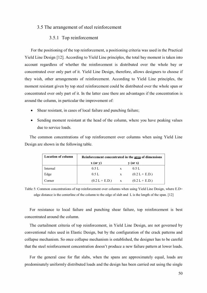
The common concentrations of top reinforcement over columns when using Yield Line
Design are shown in the following table.
Table 5: Common concentrations of top reinforcement over columns when using Yield Line Design, where E.D=
edge distance is the centerline of the column to the edge of slab and L is the length of the span. [12]
For resistance to local failure and punching shear failure, top reinforcement is best
concentrated around the column.
The curtailment criteria of top reinforcement, in Yield Line Design, are not governed by
conventional rules used in Elastic Design, but by the configuration of the crack patterns and
collapse mechanism. So once collapse mechanism is established, the designer has to be careful
that the steel reinforcement concentration doesn’t produce a new failure pattern at lower loads.
For the general case for flat slabs, when the spans are approximately equal, loads are
predominately uniformly distributed loads and the design has been carried out using the single
Location of column Reinforcement concentrated in the area of dimensions
x (or y) y (or x) Internal 0.5 L x 0.5 L
Edge 0.5 L x (0.2 L + E.D.)
Corner (0.2 L + E.D.) x (0.2 L + E.D.)

51
load case of maximum design load on all spans. Then 100% top steel may generally be curtailed
at 0.25 x span from the centerline of internal columns and 100% top steel may generally be
curtailed at a distance of 0.20 x span, at right angles to the edge, from the centerline of perimeter
columns.
3.5.2 Bottom reinforcement
The bottom reinforcement, using Yield Line Design principles, is assumed generally regular
in whole bays for the slab, without curtailment. That curtailment of bottom reinforcement is
best avoided because it is usual to assume a constant moment along the whole length of the
yield lines.
In Yield Line Design, the checks involving the localised failure modes around column
supports use the full moment of resistance of the bottom reinforcement within the areas of the
local failure patterns. It is therefore advisable not to carry out any curtailment of bottom bars in
these areas.
It may then be necessary to check whether a yield line pattern giving a lower overall load
capacity can develop along the line where the reinforcement is reduced.
Moreover, conventional detailing practice following the bending moment envelope leads to
inefficiencies in production due to:
• Different length bars increase the number of bar marks and impose a strict discipline on
their placing.
• Staggering bars of the same length also slows down the laying process.
• Changing bar diameters and their spacing to fit as closely as possible to the moment will
also effect the time needed to place the bars.
• Complex reinforcement layouts also require more checking and offer very little
flexibility.
All these points incur increased labour costs and slow down progress on site. So, for Yield
Line designs it is recommended that bottom steel reinforcement is not curtailed, and it is
positioned over the entire length of the slab span.

52
3.6 Punching shear in SFRC
The steel fibres in concrete can also considerably influence shear behavior and shear
capacity. Fibres can reduce the amount of stirrups and congestion of reinforcement in high shear
regions. Fibres do not only improve the flexural behavior but also the shear capacity. [13]
In flat slabs, punching shear failures normally develop around supported areas (columns,
capitals, walls). Punching can also result from a concentrated load applied to a relatively small
area of the structure.
The design procedure for punching shear is based on checks at the face of the column and at
the basic control perimeter 𝑢1. If shear reinforcement is required a further perimeter 𝑢𝑜𝑢𝑡,𝑒𝑓
should be found where shear reinforcement is no longer required. How it is explained in the
Eurocode [14], the following checks should be carried out:
• At the column perimeter, or the perimeter of the loaded area, the maximum punching
shear stress should not be exceeded:
𝑣𝐸𝑑 < 𝑣𝑅𝑑,𝑚𝑎𝑥 (3.22)
• Punching shear reinforcement is not necessary if:
𝑣𝐸𝑑 < 𝑣𝑅𝑑,𝐹 (3.23)
Where
𝑣𝑅𝑑,𝐹 is the design value of the punching shear resistance of a slab without punching shear
reinforcement along the control section considered.
𝑣𝑅𝑑,𝑚𝑎𝑥 is the design value of the maximum punching shear resistance along the control
section considered.
𝑣𝐸𝑑 is the maximum shear stress agent.
From a practical point of view, the influence of SFRC for shear resistance is mainly related
to the possibility of replacing all transverse reinforcement. In the “fib bulletin 57 Shear and
Punching Shear in RC and FRC Elements” [13], the equation suggested by Eurocode 2 to
compute the shear contribution in concrete members without shear reinforcement, was modified
to include the influence of fibres

53
The design punching shear resistance [MPa] of a FRC slab without punching shear
reinforcement was rearranged by adding the term 𝑓𝐹𝑡𝑢𝑘
𝛾𝐹 and may be calculated as follows:
𝑣𝑅𝑑,𝐹 = 𝑣𝑅𝑑,𝑐 + 𝑣𝑅𝑑,𝑓
𝑣𝑅𝑑,𝐹 = 𝐶𝑅𝑑,𝑐𝑘(100𝜌𝑙𝑓𝑐𝑘)1
3 + 𝑘1𝜎𝑐𝑝 +𝑓𝐹𝑡𝑢𝑘
𝛾𝐹 (3.24)
where: 𝑓𝑐𝑘 is compressive strength in MPa
𝜎𝑐𝑝 is the average stress acting on the concrete due to loading or prestressing. 𝑓𝐹𝑡𝑢𝑘 is the characteristic value of the ultimate residual tensile strength for FRC, by
considering wu = 1.5 mm [MPa]
𝑓𝑐𝑡𝑘 is the characteristic value of the tensile strength for the concrete matrix. [MPa]
𝑘 = 1 + √200
𝑑≤ 2 , d in mm
𝐶𝑅𝑑,𝑐 =0.18
𝛾𝑐
𝜌𝑙 = √(𝜌𝑙𝑥 ∙ 𝜌𝑙𝑦 ≤ 0.02, and 𝜌𝑙𝑥 , 𝜌𝑙𝑦 relate to the bonded tension steel in x- and y- directions
respectively. The values 𝜌𝑙𝑥 , 𝜌𝑙𝑦 should be calculated as mean values taking into account a slab
width equal to the column width plus 3d each side.
The code also defines a minimum value for the shear resistance, which is given by the
following equation
𝑣𝑚𝑖𝑛 = 0.035𝑘3
2𝑓𝑐𝑘
1
2 (3.25)
The shear resistance 𝑣𝑅𝑑,𝑚𝑎𝑥 is the maximum of the value 𝑣𝑅𝑑,𝑐 - 𝑣𝑚𝑖𝑛
If 𝑣𝐸𝑑 exceeds the value 𝑣𝑅𝑑,𝑐 for the control section considered, punching shear
reinforcement should be provided according the Eurocode. The design procedure for punching
shear is based on checks at the face of the column 𝑢0. and at the basic control perimeter 𝑢1. The
maximum shear stress should be taken as:
𝑣𝑒𝑑 =
𝛽𝑉𝑒𝑑
𝑢0,1𝑑 (3.26)

54
Where
𝑉𝑒𝑑 is the acting reaction in the column minus the agent external loads in the perimeter 𝑢1
𝑢0,1 is the basic control perimeter
𝑑 is the mean effective depth of the slab
𝛽 is a parameter that recommended values are given in Figure 37
Figure 38: Recommended values for β
The basic control perimeter 𝑢1 may normally be taken to be at a distance 2𝑑 from the loaded
area and should be constructed to minimise its length. It is possible to calculate it as shown in
the figure 38
Figure 39: Typical basic control perimeters around loaded areas
Where shear reinforcement is required 𝑣𝐸𝑑 > 𝑣𝑅𝑑,𝑐, it should be calculate the area of the
reinforcement in accordance with Eurocode 2:
𝑣𝑅𝑐,𝑐𝑠 = 0.75𝑣𝑅𝑑,𝑐 + 1.5 (
𝑑
𝑠𝑟) 𝐴𝑠𝑤𝑓𝑦𝑤𝑑 (
1
𝑢1𝑑) 𝑠𝑖𝑛𝛼 (3.27)

55
Where:
𝐴𝑠𝑤 is the area of one perimeter of shear reinforcement around the column [mm2]
𝑠𝑟 is the radial spacing of perimeters of shear reinforcement [mm]
𝑓𝑦𝑤𝑑 = 250 + 0.25𝑑 ≤ 400 is the effective design strength of the punching shear
reinforcement. [MPa]
𝛼 is the angle between the shear reinforcement and the plane of the slab.
Through the following equation (3.28) is possible to calculate the control perimeter at which
shear reinforcement is no required.
𝑢𝑜𝑢𝑡,𝑒𝑓 =
𝛽𝑉𝑒𝑑
𝑣𝑅𝑑,𝑐𝑑 (3.28)
56
4 Parametric studies
Parametric studies are aimed to analyse the influence of the SFRC in a flat slab. It is carried
out some parametric studies aimed to analyse the influence of the compressive and tensile
strength of the fibre reinforced concrete on flexural behavior. The ratio between the negative
and positive area of ordinary reinforcement is analysed to verify if it affects the total amount of
steel. At the end, it is studied the redistribution percentage of an elastic moment for different
cases.
It is important first of all to define the model, so the stage consists of the following previous
steps:
- Flat slab’s dimension, which can be arbitrarily set.
As a first example, it has been defined a quadratic 4x4 slab. It is considered a length of 6
meters for each span in both directions, thus obtaining 6x6m square panel. Pillars with
dimensions of 25 x 25 cm were also considered.
- Choice of the slab thickness (t) in order to limit the slab slenderness (t/L=thickness/span
length) in the range: 1
35≤
𝑡
𝐿≤
1
25
So it’s defined a thickness of 200 mm
- Definition of material properties:
The material properties of the concrete and steel reinforcement are summarized in
table 6 and 7. B500C steel and a C50/60 concrete are considered.

57
Table 6: Conventional reinforcing steel properties
Table 7: Concrete properties
In this thesis, for the tensile contribution of the concrete given by the fibres, the values
obtained from a study carried out at the University of Brescia for a technical paper [12] are
used. The following table shows the values of tensile strength for different quantities of fibres.
From the value 𝑓𝑅3𝑘 is possible to calculate the ultimate residual strength 𝑓𝐹𝑡𝑢 by the equation
(3.19)
Conventional reinforcing steel
Designation Unit B500C Modulus of elestacity
Es [MPa] 210000
Characteristic yielding strength fyk [MPa] 500
Safety factor γs [-] 1,15
Design yielding strength fyd [MPa] 434,7826
Specific weight γg [kg/m3] 7850
Concrete Designation Unit
Mean modulus of elestacity Ecm [MPa] 38629
Poisson’s coefficient [-] 0,15
Characteristic cylindrical compressive strength
fck [MPa] 50
Safety factor γc [-] 1,5
Design compressive strength fcd [MPa] 33,3
Mean tensile strength fctm [MPa] 4,07
Mean flexural tensile strength fctm,fl [Mpa] 5,7

58
Fibre dosage Fibre aspect ratio
Fibre tensile
strength Fr3k Ftu
[Kg/m3] [-] [GPa] [Mpa] [Mpa] 0
80
2
0 0 15 2,1 0,46 20 2,7 0,6 25 3,4 0,75 30 4,1 0,91 40 5,5 1,22 50 6,9 1,53 60 8,2 1,82 70 9,6 2,13
Table 8: Fibre properties [15]
- Set the arrangement of the rebars As already explained in chapter 3.5, the following arrangement in figure 39 has been
taken into account for the top reinforcement. While the bottom reinforcement is arranged
over the entire area of the slab.
Figure 40: Proposed distribution of top of reinforcement [12]

59
- Cross section
The values of resistant moment obtained refer to one meter of length of the slab and it is
considered a rebars covering of 30 cm, as shown in figure 40
- Define the cracking moment
𝑀𝑐𝑟 =𝑏ℎ2
6𝑓𝑐𝑡𝑚,𝑓𝑙 = 38 [
𝐾𝑁𝑚
𝑚]
Once the parameters of the model are defined, some studies are aimed to analyse different
important aspect.
4.1 Influence of 𝑓𝑐𝑘
First of all, it is important to point out that the compressive strength of concrete does not
significantly affect the behaviour and flexural resistance of the slab, with and without the
ordinary reinforcement. Through equations 3.7, 3.20 and 3.21 the values of the ultimate
resistant moment and the ultimate agent load are obtained. Two different values of compressive
strength equal to 30 and 50 MPa are considered. It’s showed that starting from about values of
𝑓𝑅3𝑘 higher than 6, there is a slight variation in the results. As the graph in Figure 41 shown,
for value of 𝑓𝑅3𝑘 = 9.6, corresponding to 70 𝑘𝑔/𝑚3of fibres, there is a variation of about 2
KNm2 for the moment and therefore about 0,5 MPa for the ultimate load.
d =
170
b = 1000
h =
200
Figure 41: Cross section

60
It is clearly illustrated by the above graphs how the contribution of the fibres significantly
influences the flexural strength, due to its traction contribution. In fact, as the residual tensile
strength increases, the ultimate load that the slab can resist increases. It’s also possible to notice
that with a value of fR3k=9,6 it is possible to obtain the ultimate moment value equal the
cracking moment.
Then, as shown in table 9, two different percentage of ordinary reinforcement are considered.
Table 9: Cases studied
The results obtained show that if reinforcement bars are present in the slab, the compressive
strength of the fibre-reinforced concrete has a slight influence when the percentage of
reinforcement increases, but it can be considered negligible. The following graphs, in Figure
42 and 43, show the results obtained.
Bottom Top As,b
[mm2/m]
As,t
[mm2/m]
As,t/As,b
[-]
ρs,b
[‰]
ρs,t
[‰]
fck
[MPa] CODE
Φ12/200 Φ12/200 565,5 568,5 1 2,82 2,82 30 2,82/30
Φ12/200 Φ12/200 565,5 568,5 1 2,82 2,82 50 2,82/50
Φ14/200 Φ14/200 769,7 769,7 1 3,84 3,84 30 3,84/30
Φ14/200 Φ14/200 769,7 769,7 1 3,84 3,84 50 3,84/50
0
5
10
15
20
25
30
35
40
45
0 1 2 3 4 5 6 7 8 9 10 11
M u
ltim
ate
[KN
m2 ]
-q
ult
imat
e [M
Pa]
fR3k [MPa]
Mu, fck = 30 [Mpa]Mu, fck = 50 [Mpa]qu, fck = 30 [Mpa]qu, fck = 50 [Mpa]
Figure 42: Mu – qu vs fR3k

61
In conclusion, the compressive strength doesn’t affect the flexural behaviour of a SFRC, but its
influence on fibre anchorage with the concrete matrix, so for the further studies it is considered
a compressive strength 𝑓𝑐𝑘 = 50 MPa.
4.2 Influence of 𝑓𝑅3𝑘
Keeping the same properties of the model, this study is aimed to analyse the influence of the
flexural strength and the reinforcement area ratio. It is predefined a bottom reinforcement equal
0
5
10
15
20
25
30
35
0 1 2 3 4 5 6 7 8 9 10 11
q u
ltim
ate
[MP
a]
fR3k [MPa]
2,82/30
2,82/50
3,84/30
3,84/50
0
10
20
30
40
50
60
70
80
90
100
0 1 2 3 4 5 6 7 8 9 10 11
M u
ltim
ate
[KN
m2 ]
fR3k [MPa]
2,82/30
2,82/50
3,84/30
3,84/30
Figure 44: Mu vs fR3k
Figure 43: qu vs fR3k
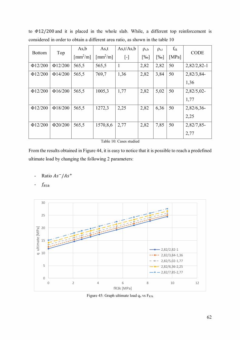
62
to 𝛷12/200 and it is placed in the whole slab. While, a different top reinforcement is
considered in order to obtain a different area ratio, as shown in the table 10
Table 10: Cases studied
From the results obtained in Figure 44, it is easy to notice that it is possible to reach a predefined
ultimate load by changing the following 2 parameters:
- Ratio 𝐴𝑠−/𝐴𝑠+
- 𝑓𝑅3𝑘
Bottom Top As,b
[mm2/m]
As,t
[mm2/m]
As,t/As,b
[-]
ρs,b
[‰]
ρs,t
[‰]
fck
[MPa] CODE
Φ12/200 Φ12/200 565,5 565,5 1 2,82 2,82 50 2,82/2,82-1
Φ12/200 Φ14/200 565,5 769,7 1,36 2,82 3,84
50 2,82/3,84-
1,36
Φ12/200 Φ16/200 565,5 1005,3 1,77 2,82 5,02 50 2,82/5,02-
1,77
Φ12/200 Φ18/200 565,5 1272,3 2,25 2,82 6,36 50 2,82/6,36-
2,25
Φ12/200 Φ20/200 565,5 1570,8,6 2,77 2,82 7,85 50 2,82/7,85-
2,77
0
5
10
15
20
25
30
0 2 4 6 8 10 12
q u
ltim
ate
[MP
a]
fR3k [MPa]
2,82/2,82-1
2,82/3,84-1,36
2,82/5,02-1,77
2,82/6,36-2,25
2,82/7,85-2,77
Figure 45: Graph ultimate load qu vs FR3k

63
In the graphs below (Figure 45 and 46), instead, it is calculated the depth of the neutral axis
and the ratio between the moments 𝑀−/𝑀+, in order to verify if the results are within the
limits (chapter 3.1).
0
0,05
0,1
0,15
0,2
0,25
0,3
0 1 2 3 4 5 6 7 8 9 10
x /
d [
-]
fR3k [MPa]
2,82/2,82-12,82/3,84-1,362,82/5,02-1,772,82/6,36-2,252,82/7,85-2,77
Figure 46: Graph ratio x /d vs fR3k
0
0,5
1
1,5
2
2,5
0 1 2 3 4 5 6 7 8 9 10
Mp-/
Mp+
[-]
fR3k [MPa]
2,82/2,82-12,82/3,84-1,362,82/5,02-1,772,82/6,36-2,252,82/7,85-2,77
Figure 47: Graph ratio Mp- / Mp+ vs fR3k

64
4.3 Influence of As-/As+
The main scope of the thesis is to optimize the amount of steel reinforcement in a flat slab,
so this study is aimed to analyse how the reinforcement area ratio influences the total amount
of rebars. How it is illustrated in table 11, this analysis is carried out for a determinate quantity
fibre (20 kg/m3 and 40 kg/m3) into the concrete and it is considered different bottom
reinforcement with three different ratios of areas. Also, in this study case, the limitations and
rules of construction present in the technical codes (chapter 3.1) are taken into consideration.
Bottom As,b
[mm2/m]
As,t
[mm2/m]
As,t/As,b
[-]
ρs,b
[‰]
ρs,t
[‰]
fR3k
[MPa]
% Fibre
content CODE
Φ10/200 392,7 392,7 1 1,96 1,96
2,7 0,83 1-2,7-0,83
Φ10/150 549,7 549,7 1 2,74 2,74
Φ12/200 565,5 565,5 1 2,82 2,82
Φ14/200 791,7 791,7 1 3,95 3,95
Φ16/200 1005,3 1005,3 1 5,02 5,02
Φ10/200 392,7 785,4 2 1,96 3,92
2,7 0,83 2-2,7-0,83
Φ10/150 549,7 1099,6 2 2,74 5,49
Φ12/200 565,5 1131 2 2,82 5,65
Φ14/200 791,7 1539,4 2 3,95 7,69
Φ16/200 1005,3 2010,6 2 5,02 10,0
Φ10/200 392,7 1570,8 4 1,96 7,85
2,7 0,83 4-2,7,0,83
Φ10/150 549,7 2199,1 4 2,74 10,9
Φ12/200 565,5 2261,9 4 2,82 11,3
Φ14/200 791,7 3078,7 4 3,95 15,4
Φ16/200 1005,3 4021,2 4 5,02 20,1
Φ10/200 392,7 392,7 1 1,96 1,96
5,5 1,66 1-5,5-1,66
Φ10/150 549,7 549,7 1 2,74 2,74
Φ12/200 565,5 565,5 1 2,82 2,82
Φ14/200 791,7 791,7 1 3,95 3,95
Φ16/200 1005,3 1005,3 1 5,02 5,02
Φ10/200 392,7 785,4 2 1,96 3,92
Φ10/150 549,7 1099,6 2 2,74 5,49

65
Table 11: Case studied
Interesting results have been obtained, which will be listed below, figure 46, 47 and 48.
Φ12/200 565,5 1131 2 2,82 5,65 5,5 1,66 2-5,5-1,66
Φ14/200 791,7 1539,4 2 3,95 7,69
Φ16/200 1005,3 2010,6 2 5,02 10,0
Φ10/200 392,7 1570,8 4 1,96 7,85
5,5 1,66 4-5,5-1,66
Φ10/150 549,7 2199,1 4 2,74 10,9
Φ12/200 565,5 2261,9 4 2,82 11,3
Φ14/200 791,7 3078,7 4 3,95 15,4
Φ16/200 1005,3 4021,2 4 5,02 20,1
0
5
10
15
20
25
30
0 10 20 30 40 50 60
q u
ltim
ate
[MP
a]
Total steel reinforcement content[kg/m3]
1-2,7-0,832-2,7-0,834-2,7-0,831-5,5-1,662-5,5-1,664-5,5-1,66
Figure 48: Graph ultimate load qu vs Total steel reinforcement content[kg/m3]

66
In the above graphs, it is possible to highlight a relevant aspect. A different ratio between
the negative and positive area of reinforcement influence the total amount of steel into the slab
and obviously the value of the ultimate load that it is possible to resist.
It can be seen from the graphs obtained that for higher ratios it is possible to obtain equal
values of ultimate load with lower values of ordinary reinforcement quantity. As shown in
figure 45, for example, if a uniformly distributed ultimate load agent of 15 MPa is considered,
a saving in reinforcement of almost 8 kg/m3 can be obtained, considering a value of fR3k =2,7
0
0,05
0,1
0,15
0,2
0,25
0,3
0,35
0,4
0,45
0 20 40 60 80 100 120 140 160 180
x /
d [
-]
Total steel reinforcement content[kg/m3]
1-2,7-0,832-2,7-0,834-2,7-0,831-5,5-1,662-5,5-1,664-5,5-1,66
Figure 49: Graph ultimate load x /d vs Total steel reinforcement content[kg/m3]
0
0,5
1
1,5
2
2,5
0 20 40 60 80 100 120 140 160 180
Mp-/
Mp+
[-]
Total steel reinforcement content[kg/m3]
1-2,7-0,832-2,7-0,834-2,7-0,831-5,5-1,662-5,5-1,664-5,5-1,66
Figure 50: Graph ultimate load Mp- / Mp+ [-] vs Total steel reinforcement content[kg/m3]

67
(20 kg/m3) or almost 3 kg/m3 with fR3k=5,5 (40 kg/m3). In any case, respecting the
requirements imposed by the standard (chapter 3.1), it is possible to obtain high values of
uniformly distributed ultimate load agent.
In conclusion, the following study highlights the influence of the area ratio of reinforcement,
so, in the optimization study, it’s important to search the optimal ratio.
4.4 Redistribution of moments
This section is aimed to analyse how the moments are redistributed from their elastic value
to the plastic one.
In statically indeterminate structures, moment distribution depends on the longitudinal
variation in stiffness and this, in turn, on the stress-strain relationships of the materials. The
most rigid sections tend to absorb more forces than the less rigid ones. So, when a section
cracks, its stiffness declines, how it is shown in figure 50, and it takes smaller moments under
increasing loads. This also occurs, but much more intensely, when a section becomes plastic
since its stiffness becomes practically negligible and it is unable to receive any further increase
in stress. [16]
In the "Practical analysis of reinforced concrete structures with moment redistribution" it is
clearly explained and illustrated how, in a qualitative way, the moments are distributed.
Figure 51: Simplified moment-curvature, M-χ, diagram [16]

68
“When the support section, which is the one subjected to the highest stress levels, reaches the cracking moment (point A), it becomes less rigid and from that instant on the load-moment relationship acquires a flatter slope while the central slope becomes steeper as it takes greater loads to maintain equilibrium (segments AB and A’B’). This continues until the span section also cracks (point B’). To accommodate further load increases, the moment distribution again
appears to behave as predicted in linear elastic analysis (segments BC y B’C’). The support
section becomes plastic at point C (hinge development), its stiffness plummets and it receives barely any bending moment, which is primarily absorbed by the central section (segments CD and C’D’). The section over the supports reaches the limit state at point D, when it takes its
ultimate moment and therefore the structure, which can resist no further loading, is regarded to have reached its limit state capacity.” [16]
It’s easy to understand by inspection figure 51.
As it is explained in the Eurocode 2[14], the moment redistribution may be performed
without verifying the plastic rotation capacity of the critical sections, and only in members
primarily subjected to bending. The maximum redistribution allowed is 30 % (0.70 ≤ δ ≤ 1.0)
if high or standard ductility steel. If the ductility of the fibres into the concrete is also taken into
account, redistribution values of more than 30 % can theoretically be assumed.
Assuming some values of top and bottom reinforcements and fR3k values, the redistribution
percentage is calculated. The values inserted in table 12 are hypothesized. The values of the
ultimate moments of the sections in the middle and at the support are obtained, using the
equations (3.20) and (3.21).
Figure 52: Evolution of deflection moment over the supports and central span sections in terms of load [16]

69
Table 12: Cases studied
Through the use of Sap2000, once an ultimate distributed load equal a 15,2 MPa is
established, the values of the elastic moment are obtained. In figures 52 and 53, it's shown the
model deployed and the elastic moments obtained.
Bottom Top As,b
[mm2/m]
As,t
[mm2/m]
As,t/As,b
[-]
ρs,b
[‰]
ρs,t
[‰] CODE
Φ12/200 Φ12/200 565,5 565,5 1 2,82 2,82 2,82/2,82-1
Φ12/200 Φ16/200 565,5 1005,3 1,77 2,82 5,02 2,82/5,02-1,77
Φ12/200 Φ18/200 565,5 1276 2,25 2,82 6,38 2,82/6,38-2,25
Figure 53: Flat slab model deployed using Sap2000

70
The mean value of the elastic moment is calculated along the support line of the central
pillars AA and along the center line of the internal panels BB. The following results are
obtained:
- 𝑀𝑒𝑙,𝑚+ = 24,3 MPa
- 𝑀𝑒𝑙,𝑚+ = 40,3 MPa
Knowing the value of the mean elastic moment for a defined distributed ultimate load, it is
possible to calculate by a linear equation, the value of the elastic moment for any load agent in
the slab. Assuming the values of positive and negative reinforcements in table 12 and different
values of fr3k, it is possible to obtain the value of positive and negative ultimate moments.
Given these values, the ultimate loads are obtained. So it’s possible to calculate the mean elastic
moment for any cases. Using equation 4.29, the percentage redistribution values of the moment
are calculated.
𝜉 =
(𝑀𝑢−𝑀𝑒𝑙,𝑚)
𝑀𝑒𝑙_𝑚 (4.29)
A B
B A
y
x
Figure 54: Elastic Moment along the y direction obtained from SAP 2000

71
The following graph in figure 54 shows the results obtained.
It is possible to observe from this graph that It’s obtained elevated redistribution values when
the ratio between the reinforcements areas is equal to 1. As the ratio increases, admissible
redistribution values instead are achieved. It is also interesting how there is an asymptotic trend
by increasing the value of the fibres.
In conclusion, it’s important to check the values of the redistribution moments in order to
guarantee structural ductility.
0
10
20
30
40
50
60
70
80
90
0 1 2 3 4 5 6 7 8 9 10
% M
om
ent
red
istr
ibu
tio
n
fR3k [MPa]
2,82/2,82-1-%ξ-2,82/2,82-1-%ξ+
2,82/5,02-1,77-%ξ-2,82/5,02-1,77-%ξ+
2,82/6,38-2,25-%ξ-2,82/6,38-2,25-%ξ-
Figure 55: Percentual moment redistribution vs fR3k

72
5 Optimization of Hybrid Flat Slab
As study of analysis, in order to find the optimal hybrid solution at ULS, the same model
used for the parametric studies developed in chapter 4 has been considered. These are briefly
summarized in the following table 13 and 14.
Table 13: Flat slab proprieties
Table 14: Fibre proprieties
After setting the design values, the ultimate agent load is calculated. As required by the EN
1992-1-1 [14], all the combinations of the design loads must be considered to obtain the most
critical values of the internal actions. The design load results from the following combination:
𝐸𝑑 = ∑ 𝛾𝐺𝐺1 + 𝛾𝐺𝐺2 + ∑ 𝛾𝑄𝜓 𝑄𝑘
𝑖
where G and Q represent permanent and variable actions respectively; the coefficients 𝛾𝑔 =
1.35, 𝛾𝑞 = 1,5 are the partial factors for actions; 𝜓 is the factor for the combination of variable
actions.
Assuming a value of thickness, which depends on span length through the equation, and the
values of dead and live load, we obtained the following design loads.
Geometry Section Materials
Concrete C50/60 Steel B500C
n° span 4x4 b [mm] 1000 fck [MPa] 50 Fyk [MPa] 500
Length spans[m] 6x6 h [mm] 200 fctm,fl [Mpa] 5,7 Fyd [MPa] 434,7
Pillars [cm] 30x30 c [mm] 30 fcd 33,3 Es [GPa] 210
Ec [Gpa] 38,6 P [kg/m3] 7850
Fibre proprieties Fibre content
[kg/m3] 0 15 20 25 30 40 50 60 70
fR3k [MPa] 0 2,1 2,7 3,4 4,1 5,5 6,9 8,2 9,6 ftu [MPa] 0 0,466 0,6 0,75 0,91 1,22 1,533 1,82 2,13
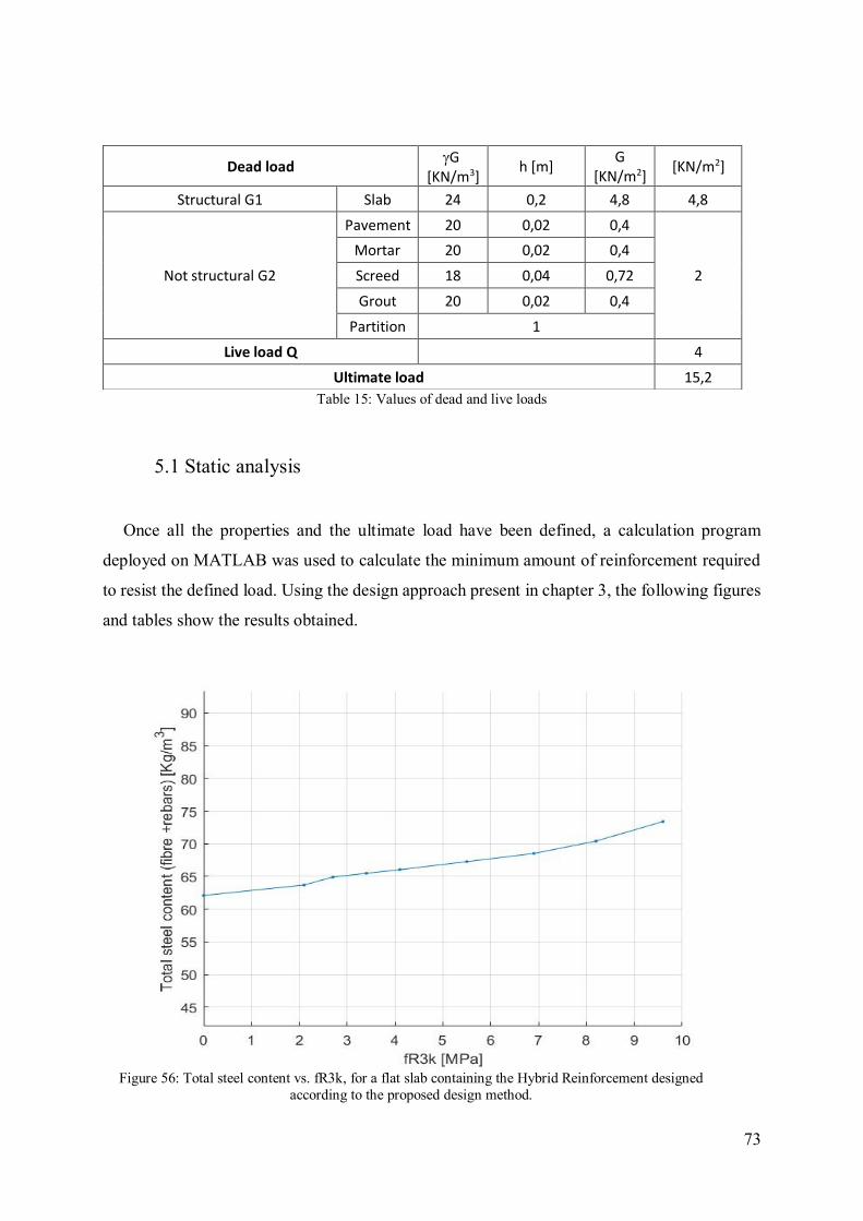
73
Table 15: Values of dead and live loads
5.1 Static analysis
Once all the properties and the ultimate load have been defined, a calculation program
deployed on MATLAB was used to calculate the minimum amount of reinforcement required
to resist the defined load. Using the design approach present in chapter 3, the following figures
and tables show the results obtained.
Dead load G
[KN/m3] h [m]
G [KN/m2]
[KN/m2]
Structural G1 Slab 24 0,2 4,8 4,8
Not structural G2
Pavement 20 0,02 0,4
2
Mortar 20 0,02 0,4
Screed 18 0,04 0,72
Grout 20 0,02 0,4
Partition 1
Live load Q 4
Ultimate load 15,2
Figure 56: Total steel content vs. fR3k, for a flat slab containing the Hybrid Reinforcement designed according to the proposed design method.
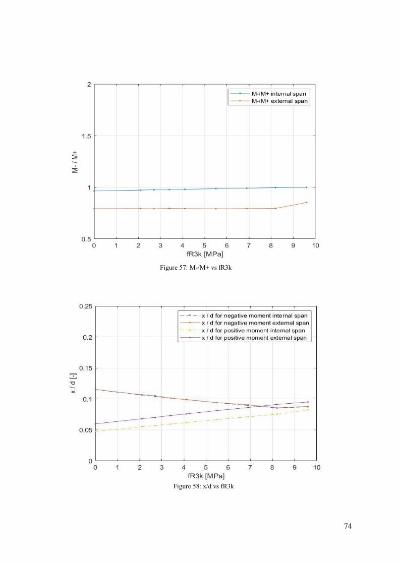
74
Figure 57: M-/M+ vs fR3k
Figure 58: x/d vs fR3k

75
Table 16: Results obtained for case analysed
From the results obtained, it can be deduced that the solution without reinforcement leads to
the optimal solution value considering all the hypotheses defined in chapter 3. There is a slight
increase in the total amount of steel when the fibre content increases. Table 16 shows that the
theoretical areas of tops obtained are almost equal, so the final amount of reinforcement in the
areas of the negative moment will be equal. While the values of bottom reinforcement in order
to obtain an optimal solution have different values.
Considering the same design approach but using the results of elastic moment obtained on
the file implemented on SAP2000, the curve fR3k vs Total steel content has been calculated
without searching the optimization value. The following moment are taken into account:
- Elastic positive moment in internal panels equal a 33MPa
- Elastic negative moment in internal panels equal a 160 MPa
- Elastic positive moment in external panels equal a 45MPa
- Elastic positive moment in external panels equal a 190 MPa
Internal spans External spans Total steel content
fR3k
[Mpa]
As,b
[mm2/m]
As,t
[mm2/m]
As,b
[mm2/m]
As,t
[mm2/m]
Fibre
[kg/m3]
Rebars
[kg/m3] Total
0 524,7 1197 639,7 1210,3 0 62.5 62.5
2,1 402,2 912,1 522,2 925,6 15 49.1 64.1
2,7 367,4 831,5 492,4 831,5 20 45.3 65.3
3,4 326,7 738,0 451,7 741,6 25 40.9 65.9
4,1 286,2 645,0 411,2 658,2 30 36.4 66.4
5,5 205,2 460,7 335,2 465 40 27.6 67.6
6,9 124,5 278,5 259,5 278,2 50 18.9 68.9
8,2 49,8 111,0 184,8 125 60 10.8 70.8
9,6 0 0 95 17 70 3.8 73.8

76
From the results obtained it is evident that using the plastic theory and therefore the yield
lines theory, it is possible to obtain an optimal solution compared to the one which would be
obtained using the design moment values of the elastic moment. A reinforcement quantity of
about 15 kg/m3 can be saved.
Even if a minimum value is not reached adding the fibres, these nevertheless have a
significant influence on the calculation of the ELS. Future studies, chapter 6, will be focused
on checking the limits of ELS with these results obtained at USL. It is to be expected that for
optimal values calculated at the ULS do not satisfy the limits imposed by the standards. So, it
probably will lead to an increase in the amount of reinforcement for low fibres content values.
Figure 59: Total steel content vs. fR3k, for plastic and elastic analysis
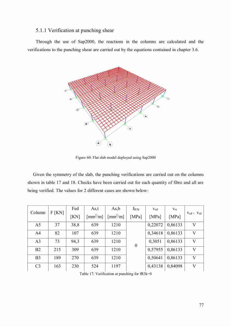
77
5.1.1 Verification at punching shear
Through the use of Sap2000, the reactions in the columns are calculated and the
verifications to the punching shear are carried out by the equations contained in chapter 3.6.
Given the symmetry of the slab, the punching verifications are carried out on the columns
shown in table 17 and 18. Checks have been carried out for each quantity of fibre and all are
being verified. The values for 2 different cases are shown below:
Table 17: Verification at punching for fR3k=0
Column F [KN] Fed
[KN]
As,t
[mm2/m]
As,b
[mm2/m]
fR3k
[MPa]
ved
[MPa]
vrc
[MPa] ved < vrd
A5 37 38,8 639 1210
0
0,22072 0,86133 V
A4 82 107 639 1210 0,34618 0,86133 V
A3 73 94,3 639 1210 0,3051 0,86133 V
B2 215 309 639 1210 0,57955 0,86133 V
B3 189 270 639 1210 0,50641 0,86133 V
C3 163 230 524 1197 0,43138 0,84098 V
Figure 60: Flat slab model deployed using Sap2000
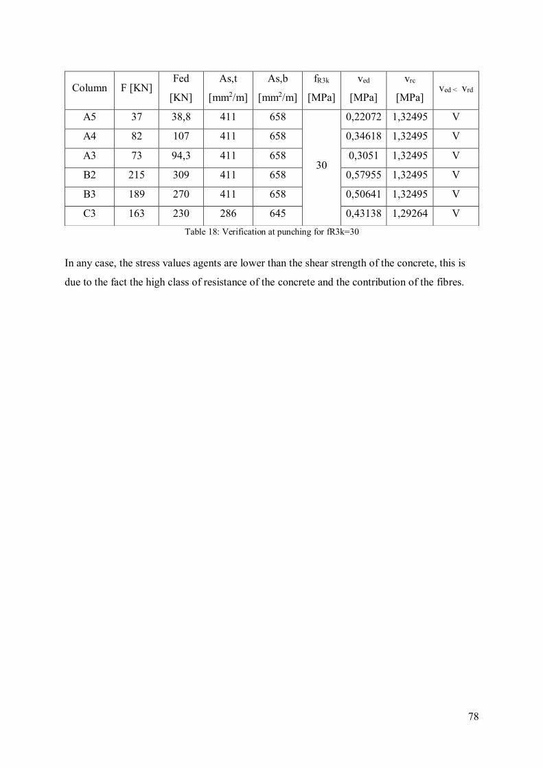
78
Table 18: Verification at punching for fR3k=30
In any case, the stress values agents are lower than the shear strength of the concrete, this is
due to the fact the high class of resistance of the concrete and the contribution of the fibres.
Column F [KN] Fed
[KN]
As,t
[mm2/m]
As,b
[mm2/m]
fR3k
[MPa]
ved
[MPa]
vrc
[MPa] ved < vrd
A5 37 38,8 411 658
30
0,22072 1,32495 V
A4 82 107 411 658 0,34618 1,32495 V
A3 73 94,3 411 658 0,3051 1,32495 V
B2 215 309 411 658 0,57955 1,32495 V
B3 189 270 411 658 0,50641 1,32495 V
C3 163 230 286 645 0,43138 1,29264 V

79
5.2 Parametric studies
Other different studies have been analysed changing some parameters keeping the previously
set values, in order to verify which value can influence the optimization.
5.2.1 Influence of ultimate load
Other different studies have been analysed changing some parameters keeping the previously
set values. First of all, it is changed the value of the live load. Using the Italian standards NTC,
it’s considered three different value of live load referred three different categories of
construction use.
- 𝑄 = 2 [Mpa] → 𝑞𝑢 = 12,2, for residential and office areas
- 𝑄 = 3 [Mpa] → 𝑞𝑢 = 13,7 , for areas susceptible to crowding, for example school and
restaurant
- 𝑄 = 4 [Mpa] → 𝑞𝑢 = 15,2, for commercial areas
Figure 61: Total steel content vs. fR3k, for different ultimate loads

80
It is possible to notice that by increasing the distributed load, the total value of the reinforcement
to be introduced obviously increases.
5.2.2 Influence of thickness of the flat slab Then, it has changed the thickness of the flat slab, always keeping in mind the relation that
limit the slab slenderness (t/L=thickness/span length) in the range: 1
35≤
𝑡
𝐿≤
1
25
Considering a length span equal a 6 m, the thickness has to be within these values
170 ≤ t ≤ 240
It has been considered three different value of thickness, for each thickness parameter, it’s
obtained the corresponding ultimate load, because of the dead load change.
- ℎ = 180 𝑚𝑚 → 𝑞𝑢 = 14,5 𝑀𝑃𝑎
- ℎ = 200 𝑚𝑚 → 𝑞𝑢 = 15,2 𝑀𝑃𝑎
- ℎ = 220 𝑚𝑚 → 𝑞𝑢 = 15,8 𝑀𝑃𝑎
The results are shown in the following Figure 61.
Figure 62: Total steel content vs. fR3k, for different thickness of the slab

81
This graph shows how the influence of the thickness of the slab affects the maximum amount
of reinforcement. It is possible to observe a high saving of steel reinforcement. However, there
are some disadvantages, as for example architectural or structural. If a building on several floors
is considered, the loads acting on the pillars are gradually higher and can, therefore, lead to a
different dimensioning of the pillars and foundations.
5.2.3 Influence of span number Another study is carried out by changing the number of spans of a building. Three cases with
three different span number cases are considered:
- 4x4
- 6x6
- 8x8
The below results are obtained in Figure 62
From the graph it can be observed that the optimization curve is lowered as the number of
spans increases. This is due to the fact that the internal panels need a lower quality of
reinforcement, therefore increasing the size of the floor, increase the number of internal panels
and therefore a reduction in kg/m3 of steel content.
Figure 63: Total steel content vs. fR3k, for different span number

82
5.2.4 Influence of fR3m
In addition, an interesting analysis has been performed, considering the average tensile
strength value of the fibres and comparing it with the values obtained considering the
characteristic values
𝑓𝑅3𝑚 =𝑓𝑅3𝑘
0.7
As it can be deduced from this graph, it is possible to deduct that an increase in the resistant
value of the fibres can lead to an optimization of the total steel content and rebars savings. So,
this last analysis shows how the quality and property of the fibres is very important in the value
of optimization. It is therefore very important to identify the best type of fibre to be used and
carry out numerous laboratory tests to obtain a characteristic value mostly reliable and accurate.
Figure 64: Total steel content for characteristic and mean tensile strength of fibre

83
5.3 Economic analysis
Another important aspect to consider is the economic aspect. In this work, only the cost of
the materials and their installation have been taken into account. The average value of the
standard €/kg of fibres is considered, which is € 1.5 with a certain deviation of 30%. As far as
reinforcement is concerned, the values are obtained from the BEDEC - ITeC - Instituto de
Tecnología de la Construcción [17], which takes into consideration the overall price of the
reinforcement, i.e. in addition to the cost of the individual material, the price for the installation
and the specialized employee have been taken into consideration. The final cost considered for
the rebars is € 1.42/kg with a certain deviation of 10%. In the following figure, it’s shown the
oscillation costs obtained.
The following graph does not lead to an economic saving, obviously because the average
cost of the fibres is higher than the cost of the reinforcement rebars.
But a key economic advantage is the reduction in construction time compared with the
traditional installation of double layers of conventional reinforcing bars, stirrups, or other shear
reinforcement. Time savings of several weeks for flat slab can be obtained; however, the
economic costs and actual savings are based on a collection of individual gains obtained and
measured using appropriate construction estimating tools and evidenced by the field data that
support the decisions made to use this construction methodology.
30
50
70
90
110
130
150
170
190
210
0 1 2 3 4 5 6 7 8 9 10
€/m
3
fR3k
Average cost
Maximum cost
Minimum cost
Figure 65. Oscillation costs [€/m3]

84
Other important aspects in this brief analysis have not been taken into account. For example the
SFRC can be directly pumped to elevated slabs, so the use of cranes for lifting reinforcing bars
is eliminated. The overall simplification of the jobsite significantly improves the physical and
labor-intensive tasks that would be otherwise needed if reinforcing bars were to be placed. This
simplification has the potential to improve safety on the jobsite. A reduction in personnel for
placing and finishing may also occur when compared with the traditional RC structures. There
is also a saving in the volume of concrete, the SFRC may be somewhat thinner than the
traditional slab when design verifications for serviceability and ultimate limit states are
assessed. In conclusion, a total cost saving is obtained for a SFRC construction compared with
traditional methods of reinforced concrete slab construction.

85
6 Conclusion
Fibre reinforcement extends the versatility of concrete as a construction material by
overcoming the otherwise intrinsic brittleness and by improving the structural behaviour (crack
propagation, flexural stiffness, ductility, ect), but also by the potential it has to simplify the
construction process.
The results presented and discussed in this thesis yield the following conclusions:
- The proposed design method provides an easy and straightforward procedure for the
designing of Hybrid Reinforcement flat slab at ULS by performing a plastic analysis of
the structure.
- The fibres give an important contribution to the flexural behaviour of the structure and
its presence in the concrete mix is able to provide the partial or even total substitution of
the conventional reinforcement due to high residual tensile strength, ductility and
toughness of the material.
- The results obtained show that using the theory of plastic for the design of a flat slab
with the design approach considered, it is possible to have a saving on the total amount
of reinforcement at ULS compared to the one that would be obtained with the values of
elastic moment.
- This design approach considered do not lead to a minimum value for different fibre
content. But by looking at the parametric studies, a minimum value is obtained if an
average value of residual tensile strength is considered or if better fibres quality is used.
6.1 Future studies
Future studies will mainly aim to verify the optimization values at the serviceability limit
state SLS, for any slab geometry and material properties. Once the best solution, that fulfil the
ULS is found, it is necessary to verify the limits imposed from the standards at SLS and in
particular the control-crack width. The technical standards impose values to be respected for
the crack width, that is closely linked to the exposure class of the structural element, in order to
ensure durability. Thanks several studies and analysis carried out, the role of the fibres in the
crack width control is known. Therefore, the optimization curve could be modified in order to
obtain all the standard requirements. Another interesting study is to find the best type of fibre
able to obtain the best optimal solution in structural and economic terms.

86
References
[1] S. M. F. Jensen and K. T. Jan Arve Øverli, “Numerical Investigation of a Post-tensioned
Flat Slab with Steel Fibre Reinforcement,” Dep. Struct. Eng, 2013.
[2] A. Abid and K. Franzen, “Design of Fibre Reinforced Concrete Beams and Slabs,” p.
128, 2011.
[3] I. Löfgren, Fibre-reinforced Concrete for Industrial Construction. 2005.
[4] A. C. I. Committee, Report on Design and Construction of Steel Fiber-Reinforced
Concrete Elevated Slabs, no. 2. 2004.
[5] K. ERICSSON, S.; FARAHANINIA, “Punching Shear in Reinforced Concrete Slabs
Supported on Edge Steel Columns,” p. 148, 2010.
[6] Model code for Concrete Structures 2010. 2013.
[7] BS EN 14651, “Measuring the flexural tensile strength (limit of proportionality (LOP),
residual),” Br. Stand. Inst., vol. 3, pp. 1–17, 2005.
[8] C. Ana Blanco ALvarez, Polit, Universitat Departament, “Characterization and
modelling of SFRC elements,” March, 2013.
[9] U. Gossla, “Development of SFRC Free Suspended Elevated Flat Slabs,” May, 2005.
[10] X. Destrée and J. Mandl, “Steel fibre only reinforced concrete in free suspended elevated
slabs: Case studies, design assisted by testing route, comparison to the latest SFRC
standard documents,” Tailor Made Concr. Struct., pp. 437–443, 2008.
[11] C. Caprani, “Civil Engineering Design ( 1 ) Analysis and Design of Slabs,” 2006.
[12] C. G. Gerard Kennedy, “Pratical yield line design,” Fiz. i Khimiya Obrab. Mater, 2003.
[13] fib, fib Bulletin 57 - Shear and Punching Shear in RC and FRC Elements, no. October.
2010.
[14] “Eurocode 2: Design of concrete structures - Part 1-1 : General rules and rules for
buildings,” no. 2, p. 227, 2004.
[15] L. Facconi, G. Plizzari, and F. Minelli, “Elevated slabs made of hybrid reinforced
concrete: Proposal of a new design approach in flexure,” Struct. Concr., vol. 20, pp. 52–
67, 2019.
[16] A. R. M. B. Andrés Doñate Megías, José Calavera Ruiz, “Practical analysis of reinforced
concrete structures with moment redistribution,” p. 89.
[17] https://itec.es/servicios/bedec/ BEDEC - ITeC - Instituto de Tecnología de la
Construcción

87
Acknowledgements
I would first like to thank Prof. Albert de La Fuente for all the time he dedicated to me and for
all the endless advice he gave me during the whole realization of this document. I will always
remember his kindness, humanity, reassurance and humor which accompanied the crucial
moments of my work.
I must express my gratitude to Stanislav Aidarov (PhD), whose role in this document has been
fundamental. I will never forget his limitless patience and passion for supervising me. His
valuable knowledge was kindly made available to me in the crucial points of the thesis.
I am grateful to Prof. Maurizio Taliano for having given me the opportunity to take this exciting
path abroad.
I will always carry in my heart all the people I met during my experience in Barcelona, all the
friends I made, who have made me fall in love with this beautiful city and country. It thanks to
them that I grew up and I opened my mind.
My thanks also go to my lifetime friends. I have always appreciated their deep affection.
Finally, I want to thank the most important persons, my parents and my brother, for the trust
and love they give me. They have always supported me in these years in every choice I made
and I am sure they will still support me in every single step I will make in the future. I want to
say to them a big "vi voglio bene".