Embed Size (px)
Citation preview

Politecnico di Torino
Porto Institutional Repository
[Article] Identification and Correction of Artifact in the Measurement of PulsedMagnetic Fields
Original Citation:Giaccone, Luca; Giordano, Domenico; Crotti, Gabiella (2017). Identification and Correctionof Artifact in the Measurement of Pulsed Magnetic Fields. In: IEEE TRANSACTIONS ONINSTRUMENTATION AND MEASUREMENT, vol. 66 n. 6, pp. 1260-1266. - ISSN 0018-9456
Availability:This version is available at : http://porto.polito.it/2674305/ since: June 2017
Publisher:Institute of Electrical and Electronics Engineers Inc.
Published version:DOI:10.1109/TIM.2017.2652739
Terms of use:This article is made available under terms and conditions applicable to Open Access Policy Article("Public - All rights reserved") , as described at http://porto.polito.it/terms_and_conditions.html
Porto, the institutional repository of the Politecnico di Torino, is provided by the University Libraryand the IT-Services. The aim is to enable open access to all the world. Please share with us howthis access benefits you. Your story matters.
(Article begins on next page)

Post-print of the paper
Identification and Correction of Artifact in the Measurement of Pulsed Magnetic
Fields, IEEE Transactions on Instrumentation and Measurement, Vol. 66, n. 6, pp.
1260–1266, 2017, DOI: 10.1109/TIM.2017.2652739
Identification and correction of artefact in the
measurement of pulsed magnetic fields
Luca Giaccone1∗, Domenico Giordano2 and Gabiella Crotti2
1 - Politecnico di Torino, Dipartimento Energia, corso Duca Degli Abruzzi, 24 - 10129 Torino
2 - Istituto Nazionale di Ricerca Metrologica, Strada delle Cacce 91, 10135, Torino, Italy
Abstract
AC magnetic flux density meters usually integrate a high pass filterwith a very low cut-off frequency (1 Hz - 30 Hz) aiming at reducing the ef-fect of slow oscillations. This can distort the actual time domain behaviourof magnetic flux density waveforms detectable close to industrial or medi-cal devices, even causing artefact high amplitude oscillations. This paperproposes a procedure to identify the filter parameters that accurately re-produce its measured frequency behaviour and suggests an algorithm tocorrect, in time domain, the field meter recorded waveform. Identificationand correction procedure are extensively tested on magnetic flux densitywaveforms provided by a system for the generation of standard magneticfields. Finally, the uncertainty associated with the identification and cor-rection procedure are assessed by means of the Monte Carlo method. As-suming an overall standard uncertainty associated with the MCM modelinputs of 0.3 %, a standard uncertainty of 0.75 % associated with the meansquare error between measured and reconstructed waveforms is obtained.
keywords: Measurement, pulsed magnetic fields, optimisation, identifica-tion, dosimetry.
1 Introduction
The measurement of pulsed magnetic fields is of high interest to severals sectors.Laboratory and commercial magnetic flux density meters can be found for thispurpose. However, they often integrate high pass filter with a very low cut-offfrequency aiming at reducing the effect of slow oscillations. In this paper weanalyse the behaviour of a magnetic flux density meter largely employed forapplications where the human exposure is the main concern. This meter hasthree selectable cut-off frequencies: 1 Hz, 10 Hz and 30 Hz. Even using thelowest one (1 Hz), possible artefact can be observed on the measured waveform.Basically, the original waveform is distorted and the degree of distortion de-pend on the shape of the original waveforms. The distortion could introduce
∗Contact: [email protected]

unacceptable systematic error in EMC or dosimetric measurement. To give anexample, complex and pulsed magnetic fields have to be assessed with suitablemethodologies [1, 2, 3, 4]. This reference [5] summarises most of the availablemethods classifying them as time domain or frequency domain based. Differentparameters are taken into account to asses the stability of the methods (offset,noise, sampling rate, signal truncation) and it is shown that some methods aremore robust with reference to some disturbances and weaker with reference toothers. Pros and cons of each method are highlighted. Bearing all this in mind,it is a matter of fact that a distortion of the original waveform could influencelater analysis based on the measurement (e.g. an exposure assessment). Thispaper focuses on quasi-rectangular waveforms because they can be found inseveral applications like, for instance, spot welding [6, 7, 8] and MRI [9, 10, 11].
An example of a pulsed magnetic field is given in Fig. 1. The actual wave-form is made of three consecutive quasi-rectangular pulses. The high pass filterdistorts the actual waveform and the measurement output is the blue curve.Three main issues are clearly observed: 1) the real pulsed nature of the originalwaveform is lost 2) the maximum registered value is higher than the true one,3) if the blue curve is used to compute the spectrum (apart from the filteredspectral content already discussed) it is not clear how to perform the signaltruncation obtaining a result that is likely affected by spectral leakage [12, 13].
This paper addresses these issues proposing a procedure to identify the filterparameters that best reproduce the measured frequency behaviour of the meter.The model of the filter is then used to simulate the artefact related to the differ-ent cut-off frequencies. The input for the model is a reference waveform providedby the Italian reference system for the generation of standard magnetic fields upto 100 kHz [14]. The output of the model is compared with the measurement ofthe meter obtaining good agreement. Furthermore, it is suggested an algorithmto correct, in time domain, the distorted waveform. The correction procedure isagain applied to the waveform measured by the meter obtaining a satisfactorycomparison with the reference waveform. In the end, the uncertainty of theidentification and correction procedure is assessed by means of the Monte Carlomethod [15, 16].
2 Filter characterisation and identification
The experimental frequency characterisation of the magnetic field meter is car-ried out by using the INRIM system for the generation of standard magneticfields up to 100 kHz [14]. A chain constituted by a Fluke 5500 calibrator and a100 A−100 kHz Clarke-Hess trans-conductance amplifier supplies the Helmholtzcoil pair. The maximum magnetic flux density which can be generated in thesystem center is 430 µT. A 24 bit, 50 kHz National Instrument DAQ boardperforms the synchronous acquisition of the meter output signals and the cur-rent flowing in the Helmholtz system. A Python program, which manages theautomatic supply frequency sweep, also performs the peak identification andthe phase displacement of the meter signals (the current signal is the refer-
2

Figure 1: Artefact example. The actual waveform is made of three consecutivequasi-rectangular pulses (red). The high pass filter distorts the actual waveform(blue).
ence for the phase) through a four-parameter sine fitting. By replacing thevoltage calibrator with an arbitrary waveform generator, the system is ableto generate arbitrary magnetic flux density waveforms. This allows the mea-surement of magnetic flux density meter capabilities under realistic distorted,quasi-rectangular or pulsed waveforms.
The magnetic field meter under study incorporates three band-pass filterswith different values of the lower cut-off frequency: 1 Hz, 10 Hz and 30 Hz.The higher cut-off frequency is 400 kHz for all the filters. This paper focuseson the measurement of quasi rectangular waveforms whose spectrum includescomponents close to the lower cut-off frequency. For this reason, the frequencyresponse of the magnetic field meter is characterised experimentally in the range0.5 Hz - 300 Hz. Fig. 2 provide the measured Bode plot for the three filters.In this range they behave as a high-pass filter showing a trend similar to athird-order filter.
Since the manufacturer does not provide detailed information on the band-pass filter used (only upper and lower cut-off frequency) we make the assumptionthat it can be modelled by means of the third order Butterworth filter repre-sented in Fig. 3. To identify the filter, parameters C1, L2 and C3 have to befound. The identification is performed with a two steps approach: 1) preliminary
3

Figure 2: Characterisation of the three filters related to the lower cut-off fre-quencies: 1 Hz, 10 Hz and 30 Hz.
Figure 3: Third order Butterworth filter used to approximate the actual highpass filter of the magnetic flux density meter.
identification with a heuristic method, 2) final identification with a determinis-tic method. The selected heuristic method is the genetic algorithm (GA) thatallows a good exploration and exploitation of the solution space [17] but it doesnot assure to reach the global optimum. After the GA, the deterministic algo-rithm called pattern search (PS) is used in order to ensure the identification ofthe global optimum [18]. The PS method needs an initial solution to perform
4

the analysis. In this paper we use as initial solution the one provided by theGA.
In both cases the algorithm minimises the mean square deviation betweenButterworth and measured gain. The objective function is defined as:
OF =
√∑j
(Gj,B −Gj,mes)2
(1)
being:
• j the index of the jth frequency,
• Gj,B the gain of the Butterworth filter at the jth frequency,
• Gj,mes the measured gain of the meter filter at the jth frequency.
The OF does not use information about the phase and, hence, they have to bechecked at the end of the process (as will be shown later).
The whole process is run several times to check the stability of the finalresults. It is found that the use of the two steps approach makes the identifica-tion really stable and independent of the GA parameters used (population size,crossover, mutation factors). Such parameters can only influence the elapsedtime but not the final result that always converges to the same optimal values.It must be stressed, however, that the GA has the key role of identifying thelocal optimum used by the PS as initial solution. Without this information theprocedure can fail leading to a non global optimum.
The optimal parameters are summarised in Table 1 for all the filters. Fig. 4compares the frequency characterisation of the meter and the Butterworth filterfrequency response obtained with the identification. For the sake of shortness,this comparison is provided only for the lowest cut-off frequency (fcut = 1 Hz). Itis apparent that the Butterworth filter approximates the actual filter with goodagreement. A slightly higher error is found for the phase at lower frequencies.This deviation is likely caused by the main assumption that approximates theactual filter with a Butterworth filter. However, we will shown later that thisdeviation does not compromise the final goal of our analysis.
Table 1: optimal parameters of the Butterworth filter
optimal optimal optimalparameter value value value
fcut = 1 Hz fcut = 10 Hz fcut = 30 Hz
C1 675.06 mF 33.70 mF 10.02 mFL2 236.79 mH 10.36 mH 3.76 mHC3 106.73 mF 10.56 mF 3.35 mF
5

Figure 4: Result of the fitting with cut-off frequency equal to fcut = 1 Hz.Measured frequency response vs. Butterworth frequency response.
3 Artefact modelling
The robustness of the identification is tested trying to reproduce the measure-ment artefacts. The same system described in Sec. 2 is used to generate a quasi-rectangular periodic waveform with fundamental frequency of 10 Hz. Fig. 5shows the magnetic flux density waveform together with its spectrum. It is ap-parent that, depending on the filter used, a significant portion of the spectrum isattenuated of even cancelled. The reference waveform is measured by a fluxgatemagnetometer and it will be used for comparison in the rest of the paper.
The modelling of the artefacts is performed solving a system of three differ-ential equations related to the Butterworth in Fig. 3:
dv1dt
=vin − v1 − v3
RC1(2)
di2dt
=vin − v3L2
(3)
dv3dt
=vin − v1 − v3
RC3+
i2C3
(4)
In equations (2), (3) and (4) the term vin corresponds to the reference field wave-form represented in Fig. 5. Once the three differential equation are solved, one
6

Figure 5: Quasi-rectangular periodic waveform with fundamental frequency of10 Hz (a). Spectrum of the waveform. (b).
can compute the output voltage as vout = vin − v1 − v3. This term correspondsto the magnetic flux density waveform distorted by the meter.
Simulations are performed for all the filters incorporated in the meter. Re-sults are provided in Fig. 6, Fig. 7 and Fig. 8 for the cut-off frequencies of 1Hz, 10 Hz and 30 Hz, respectively. The red curve is the reference waveform, thegreen curve is the waveform measured by the meter and the blue (dashed) oneis the simulation. In all figures three cycles are magnified to make easier thecomparison. It is apparent that a good agreement is found for all the filters.
4 Correction procedure
In this section the attention is focused on a more interesting aspect related tothe use of the identified filters. Since the identification has been proven to bereliable in previous sections, one can attempt to use it for the correction ofthe distorted waveform obtaining the true one (without artefacts). The set of
7
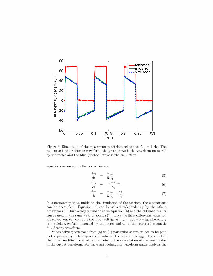
Figure 6: Simulation of the measurement artefact related to fcut = 1 Hz. Thered curve is the reference waveform, the green curve is the waveform measuredby the meter and the blue (dashed) curve is the simulation.
equations necessary to the correction are:
dv1dt
=voutRC1
(5)
di2dt
=v1 + vout
L2(6)
dv3dt
=voutRC3
+i2C3
(7)
It is noteworthy that, unlike to the simulation of the artefact, these equationscan be decoupled. Equation (5) can be solved independently by the othersobtaining v1. This voltage is used to solve equation (6) and the obtained resultscan be used, in the same way, for solving (7). Once the three differential equationare solved, one can compute the input voltage as vout = vout+v1+v3, where, voutis the field waveform distorted by the meter and vin is the corrected magneticflux density waveform.
When solving equations from (5) to (7) particular attention has to be paidto the possibility of having a mean value in the waveforms vout. The effect ofthe high-pass filter included in the meter is the cancellation of the mean valuein the output waveform. For the quasi-rectangular waveform under analysis the
8

Figure 7: Simulation of the measurement artefact related to fcut = 10 Hz. Thered curve is the reference waveform, the green curve is the waveform measuredby the meter and the blue (dashed) curve is the simulation.
mean value is completely cancelled after one single cycle. During the correctionprocess one has to select a portion of the waveform that does not present amean value, otherwise the three sequential integral will lead to waveform thatvaries with the third power of the time superposed on true waveform. Finally,technically speaking, even after the selection of a waveform without a meanvalue, it is better to numerically remove possible very small mean values comingfrom the signal truncation.
4.1 Correction procedure applied to quasi-rectangular wave-forms
The correction procedure has been successfully applied to the measured wave-forms presented in previous section. Fig. 9, Fig. 10 and Fig. 11 provide thecomparison for the cut-off frequencies of 1 Hz, 10 Hz and 30 Hz, respectively.They all include the reference waveform (red), the waveform measured by themeter (green), and the corrected waveform in (blue, dashed). It is worth notingthat the correction procedure based on the removal of the mean values provides,obviously, a result without a mean value as well. The corrected waveforms pre-sented in figures from 9 to 11 are obtained imposing, at the end of the correction
9

Figure 8: Simulation of the measurement artefact related to fcut = 30 Hz. Thered curve is the reference waveform, the green curve is the waveform measuredby the meter and the blue (dashed) curve is the simulation.
process, that the waveform starts from zero.
4.2 Correction procedure applied to a real case study:MFDC spot welding gun
The correction procedure is finally tested on a magnetic flux density waveformmeasured close to a medium frequency direct current welding gun. The magneticfield is pulsed and the highest frequency of the spectrum is approximately 10 kHz[7]. This kind of waveform is clearly subject to the measurement issues describedin this paper. Fig. 12 provides in red the measured waveform using the filterwith the lowest cut-off frequency, fcut = 1 Hz. By processing this waveformwith the correction procedure the blue curve is obtained. The lowest subfiguremagnifies the time range during the slope-up of the magnetic flux density inorder to appreciate the quality of the correction.
From the technical point of view, the blue curve is obtained removing themean value before the integration in time domain. The result is then shifted upknowing that the waveform starts from zero. This knowledge comes from thefact that the magnetic flux density is proportional to the welding current thatwas measured as well during the pulse.
10

Figure 9: Test of the correction procedure on the measured waveform withfcut = 1 Hz. The red curve is the reference waveform, the green curve isthe waveform measured by the meter and the blue (dashed) curve waveformobtained by means of the correction procedure.
5 Uncertainty
The uncertainty associated to the standard deviation between the measuredand corrected magnetic flux density signals can be estimated by a applying aMonte Carlo method (MCM) [15, 16]. The correction procedure is based on theidentification of the filter parameters and, consequently, on the measurementof the frequency characterisation of the filter (gain and phase). The MCM isapplied to the following model: 1) identification of the filter, 2) applicationof the correction procedure, 3) computation of the mean square error betweencorrection and reference signal. Since the inputs of the MCM come from ameasurement procedure, the associated probability density function (pdf) hasa gaussian shape.
It is important to highlight that the pdf associated with the MCM outputactually involves both the output of the propagated uncertainty of the complextransfer function and the repeatability of the identification stage of the model.Moreover, the obtained information is only a part of the overall uncertaintyassociated with the magnetic flux density quantity, which is the actual mea-surand. In a complete uncertainty budget, the meter uncertainty, the actualenvironmental conditions, the magnetic flux density uniformity, etc... have to
11
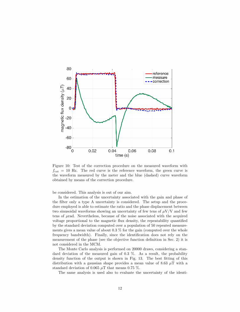
Figure 10: Test of the correction procedure on the measured waveform withfcut = 10 Hz. The red curve is the reference waveform, the green curve isthe waveform measured by the meter and the blue (dashed) curve waveformobtained by means of the correction procedure.
be considered. This analysis is out of our aim.In the estimation of the uncertainty associated with the gain and phase of
the filter only a type A uncertainty is considered. The setup and the proce-dure employed is able to estimate the ratio and the phase displacement betweentwo sinusoidal waveforms showing an uncertainty of few tens of µV/V and fewtens of µrad. Nevertheless, because of the noise associated with the acquiredvoltage proportional to the magnetic flux density, the repeatability quantifiedby the standard deviation computed over a population of 50 repeated measure-ments gives a mean value of about 0.3 % for the gain (computed over the wholefrequency bandwidth). Finally, since the identification does not rely on themeasurement of the phase (see the objective function definition in Sec. 2) it isnot considered in the MCM.
The Monte Carlo analysis is performed on 20000 draws, considering a stan-dard deviation of the measured gain of 0.3 %. As a result, the probabilitydensity function of the output is shown in Fig. 13. The best fitting of thisdistribution with a gaussian shape provides a mean value of 8.63 µT with astandard deviation of 0.065 µT that means 0.75 %.
The same analysis is used also to evaluate the uncertainty of the identi-
12

Figure 11: Test of the correction procedure on the measured waveform withfcut = 30 Hz. The red curve is the reference waveform, the green curve isthe waveform measured by the meter and the blue (dashed) curve waveformobtained by means of the correction procedure.
fication procedure. At each run of the MCM the value of C1, L2 and C3 isregistered. The best fitting of their distribution with a gaussian shape providesthe results summarised in Table 2. The same table summarises also the resultsfor the mean square error presented above.
Table 2: Uncertainty of identification and correction procedure
meanstandard standard
parameter deviation deviationµ σ (%)
C1 675.36 mF 21.47 mF 3.179L2 236.89 mH 2.06 mH 0.870C3 106.73 mF 0.18 mF 0.169
MSE 8.63 µT 0.065 µT 0.753
13

Figure 12: Correction of the magnetic flux density waveform generated by awelding gun. Measurement in red and correction in blue.
6 Conclusion
When an AC magnetic flux density meter is employed in the detection of pulsedsignals, time domain artefact can occur. This could introduce unacceptablesystematic error in EMC or dosimetric measurement purposes. In this paperwe extend the preliminary work presented in [19]. We analyse the behaviourof a magnetic flux density meter largely employed for applications where thehuman exposure is the main concern. This meter has three selectable cut-offfrequencies: 1 Hz, 10 Hz and 30 Hz. The three filters are characterised showingthe classical trend of a third order high pass filter. We propose an identificationprocedure based on a two steps approach (heuristic + deterministic) that isshown to be effective and reliable. The identified parameters allow to accuratelymodel the meter behaviour and to develop a correction procedure that makespossible to compute the true waveform starting from the measured (distorted)one. The correction procedure is tested with two different waveforms: 1) aquasi-rectangular periodic waveform provided by a system for the generationof standard magnetic fields, 2) a pulsed waveform generated by a spot weldingdevice. In both cases a satisfactory correction is obtained.
Finally, the uncertainty of the identification and correction procedure is eval-uated by means of the Monte Carlo method. Starting from the frequency char-acterisation of the filter affected by a standard uncertainty of 0.3 % it is founda standard uncertainty of the correction procedure of 0.75 % which correspondto an expanded uncertainty of 1.5% (coverage factor = 2). This figure, which
14

Figure 13: Probability density function of the mean square error related to thecorrection procedure. The best fitting of this distribution with a gaussian shapeprovides a mean value of 8.63 µT with a standard deviation of 0.065 µT thatmeans 0.75 %.
has to be considered as a contribution to the uncertainty budget associatedwith on-site magnetic flux density measurement, gives a negligible contributioncompared with the expanded uncertainty which generally is around 10%.
References
[1] K. Jokela, “Restricting exposure to pulsed and broadband magnetic fields,”Health Phys, vol. 79, no. 4, pp. 373–388, 2000.
[2] ICNIRP, “Guidance on determining compliance of exposure to pulsed andcomplex non-sinusoidal waveform below 100 kHz with icnirp guidelines,”Health Phys, vol. 84, no. 3, pp. 383–387, 2003.
[3] ICNIRP, “Guidelines for limiting exposure to time-varying electric andmagnetic fields (1 Hz to 100 kHz),” Health Phys, vol. 99, no. 6, pp. 818–836,2010.
15

[4] “Non-binding guide to good practice for implementing Directive2013/35/EU - Electromagnetic Fields - Volume 1: Practical Guide,” ISBN:978-92-79-45869-9, DOI: 10.2767/961464, 2015.
[5] V. De Santis, X. L. Chen, I. Laakso, and A. Hirata, “On the issues related tocompliance of LF pulsed exposures with safety standards and guidelines,”Phisycs in Medicine and Biology, vol. 58, pp. 8597–8607, 2013.
[6] A. Canova, F. Freschi, L. Giaccone, and M. Repetto, “Exposure of workingpopulation to pulsed magnetic fields,” IEEE Transaction on Magnetics,vol. 46, no. 8, pp. 2819–2822, 2010.
[7] A. Canova, F. Freschi, L. Giaccone, and M. Manca, “A simplified procedurefor the exposure to the magnetic field produced by resistance spot weldingguns,” IEEE Transaction on Magnetics, vol. 52, no. 3, art. num 5000404,2016.
[8] “EN 50505 - Basic standard for the evaluation of human exposure to electro-magnetic fields from equipment for resistance welding and allied processes.”
[9] F. Hennel, F. Girard, and T. Loenneker, “”Silent” MRI with soft gradientpulses.,” Magnetic resonance in medicine, vol. 42, pp. 6–10, jul 1999.
[10] H. Han, A. V. Ouriadov, E. Fordham, and B. J. Balcom, “Direct measure-ment of magnetic field gradient waveforms,” Concepts in Magnetic Reso-nance Part A, vol. 36A, pp. 349–360, nov 2010.
[11] D. Giordano, M. Borsero, G. Crotti, and M. Zucca, “Analysis of magneticand electromagnetic field emissions produced by a MRI device,” Proc. 17thSymp. Imeko TC4, p. 86.
[12] T. Grandke, “Interpolation Algorithms for Discrete Fourier Transforms ofWeighted Signals,” IEEE Transactions on Instrumentation and Measure-ment, vol. 32, pp. 350–355, jun 1983.
[13] D. Bellan, A. Gaggelli, F. Maradei, A. Mariscotti, and S. Pignari,“Time-Domain Measurement and Spectral Analysis of Nonstationary Low-Frequency Magnetic-Field Emissions on Board of Rolling Stock,” IEEETransactions on Electromagnetic Compatibility, vol. 46, pp. 12–23, feb 2004.
[14] M. Chiampi, G. Crotti, and D. Giordano, “Set up and characterization of asystem for the generation of reference magnetic fields from 1 to 100 kHz,”Instrumentation and Measurement, IEEE Transactions on, vol. 56, no. 2,pp. 300–304, 2007.
[15] Joint Committee for Guides in Metrology, “JCGM 101 – Evaluation ofmeasurement data – Supplement 1 to the ”Guide to the expression of un-certainty in measurement” – Propagation of distributions using a MonteCarlo method (ISO/IEC Guide 98-3-1),” 2008.
16

[16] O. Bottauscio, M. Chiampi, G. Crotti, D. Giordano, W. Wang, and L. Zil-berti, “Uncertainty estimate associated with the electric field induced insidehuman bodies by unknown lf sources,” IEEE Transactions on Instrumen-tation and Measurement, vol. 62, pp. 1436–1442, June 2013.
[17] J. H. Holland, Adaptation in Natural and Artificial Systems. Ann Arbor,MI: The Univ. of Michigan Press, 1975.
[18] R. Hooke and T. A. Jeeves, ““Direct search” solution of numerical andstatistical problems,” Journal of the Association for Computing Machinery,vol. 8, no. 2, pp. 212–229, 1961.
[19] G. Crotti, L. Giaccone, and D. Giordano, “Identification and correction ofartefact in the measurement of pulsed magnetic fields,” in Conference onPrecision Electromagnetic Measurements, CPEM, Ottawa, Canada, 10-15July 2016.
Authors’ Biographies
Luca Giaccone (SM’15) was born in Cuneo, Italy, in 1980.He received the Laurea degree and the Ph.D. degree in Elec-trical Engineering from the Politecnico di Torino, Turin,Italy, in 2005 and 2010, respectively. Dr. Giaccone worked onseveral areas of the electrical engineering: optimisation andmodelling of complex energy systems, computation of elec-tromagnetic and thermal fields, energy scavenging, magneticfield mitigation, EMF dosimetry, compliance of LF pulsedmagnetic field sources. Since 2011 he is assistant professorwith the Politecnico di Torino, Dipartimento Energia. He is
member of the IEEE since 2014 and he has been elevated to senior member inFebruary 2015. Since November 2015 he is member of the IEEE InternationalCommittee on Electromagnetic Safety - TC 95 - SC6 EMF Dosimetry Modeling.
Domenico Giordano received the Ph.D. degree in elec-trical engineering from the Politecnico of Torino, Torino,Italy, in May 2007. From 2007 to 2009, he collaborated withIstituto Nazionale di Ricerca Metrologica (INRIM), Torino,with a postdoctoral research grant. Since 2009, he has beenwith the Electromagnetics Division, INRIM. His research in-terests include the evaluation of human exposure to magneticfields generated by nonsinusoidal and impulsive sources andstudies of procedures for the calibration of magnetic field me-ters, on the study of ferroresonance phenomena and on the
development and characterization of voltage transducers for on-site calibrationand power quality measurements on the medium-voltage grid.
17

Gabriella Crotti received the M.S. degree in physicsfrom the University of Torino, Torino, Italy, in 1986. She isa Chief Technologist in the Electromagnetics Division, Isti-tuto Nazionale di Ricerca Metrologica (INRIM), Torino. Herresearch interests include the development of references andmeasurement techniques of high voltages, high currents, andlow and intermediate-frequency electromagnetic fields.
18