Political Constraints on Legal Doctrine:How Hierarchy Shapes the Law

Jeffrey R. LaxDepartment of Political Science

Columbia UniversityJRL2124@columbia.edu

February 28, 2012

Abstract

When higher court judges attempt to assert control over lower-court decision-making, dosuch hierarchical politics shape legal doctrine? Using a “case-space” model of choice betweendeterminate doctrines (rules) and more flexible doctrines (standards), I argue that the structureof doctrine affects the application of and compliance with doctrine by lower courts, and thisin turn affects choice among doctrinal structures. Doctrinal choice, legal complexity, lowercourt discretion, and the allocation of judicial resources are shown to depend on hierarchicalconflict, the transparency of decisions, sensitivity to case facts, judicial expertise, salience, andissue complexity. These incentives have counterintuitive effects on lower court discretion andon doctrinal specificity, and they create odd patterns of ideological and doctrinal alignment.Ignoring these incentives undercuts our understandings of lower court compliance, of judicialideology, and of the effects of collegiality on law.1

1Forthcoming 2012, Journal of Politics. For helpful comments, I thank Jenna Bednar, Matt

Behncke, Deborah Beim, Bernard Black, Charles Cameron, Cliff Carrubba, Tom Clark, Stu Jordan,

John Kastellec, David Primo, Kevin Quinn, Kelly Rader, Jim Rogers, Dan Rodriguez, Matthew

Spitzer, Deborah Weiss, and Travis Wofford, as well as participants at the Law and Positive Polit-

ical Theory Conference at the University of Rochester, at the Political Economy and Public Law

Conference at Harvard University, at the USC Center in Law, Economics, and Organization, and

at the Law and Economics Workshop at the University of Texas Law School. The online appendix

contains supplemental results and robustness checks.

The Supreme Court and the lower federal courts play distinct roles in the production of le-

gal policy. The top tier of a judicial hierarchy concentrates far more on doctrine—rule creation

and articulation—while the bottom tier concentrates on application of rules to specific cases. As

(Shapiro 2006, 273) puts it, the Supreme Court itself does not “routinely apply the rules and stan-

dards it announces. Instead, the Court has cast itself in an ‘Olympian’ role—announcing rules and

standards from on high.” The justices of the Supreme Court rely on the legal opinions they hand

down as vehicles for their legal policy goals; the judges on the Courts of Appeals (the middle level

of the federal judicial hierarchy) rely on their opinions to govern dispute resolution by the district

court judges (the bottom tier). Lower court judges can disagree with their hierarchical superiors

about case outcomes and the rules determining them, for reasons of ideology or legal philosophy.

Even when the lower courts are largely aligned with the higher court or simply seek to obey their

superiors, it may still be difficult for the higher court to convey exactly what it wants in the full

range of possible cases that can arise. How do the content and structure of legal doctrine affect

compliance and rule application in the lower courts? And, as higher court judges construct le-

gal doctrine to best get the case outcomes they want, does reliance on hierarchical application of

doctrine affect choice of doctrine in the first place? In short, do hierarchical politics shape law?

I argue that they do, and show why and how. I study the politics of rule making in the face of

hierarchical doctrinal application—in particular, the incentives driving the choice between deter-

minate doctrines (bright-line rules) and flexible or indeterminate doctrines (standards).

Perhaps the best known bright-line rule is that suspects must be informed of their rights, Mi-

randa v. Arizona (1966). Related cases establishing bright-line rules include Davis v. U.S. (1994)

requiring suspects to explicitly request counsel after Miranda warnings and Berghuis v. Thompkins

(2010) requiring suspects to explicitly invoke the right to silence Heytens (2008, 2094) gives other

criminal procedure examples of bright-line rules and of such rules replacing previous standards. In

other cases, the Court has rejected a bright-line approach in favor of a standard, even in the same

1

areas of the law or for seemingly analogous questions. Fare v. Michael C. (1979) established a

“totality of the circumstances” test for juvenile waiver of Fifth Amendment rights mandating “eval-

uation of the juvenile’s age, experience, education, background, and intelligence, and into whether

he has the capacity to understand the warnings given him.” Bellotti v. Baird (1979) invoked a

maturity standard and explicitly rejected a bright-line calendar age rule for unmarried women un-

der 18 seeking an abortion without parental consent. This same form of evaluation was rejected,

however, in Thompson v. Oklahoma (1988), wherein the plurality instead barred execution of

offenders under 16. This bright-line rule was extended to those under 18 in Roper v. Simmons

(2005), overruling Stanford v. Kentucky (1989), which had allowed execution of those under 18

and over 16. The justices sometimes make their disagreements over doctrinal type explicit. In

Miranda, Justice Clark wrote separately opposing a bright-line rule in favor of a “totality of the

circumstances” standard. Returning to the issue of death sentences for minors, in Stanford, Justice

O’Connor wrote a concurrence arguing a proportionality analysis should be conducted, but still

joined parts of the majority opinion, agreeing with the conservative plurality that there was no bar

against the execution of those 16 and 17 years of age. Justice Brennan, dissenting on behalf of

the liberal minority, argued that “the Eighth Amendment requires that a person who lacks that full

degree of responsibility for his or her actions associated with adulthood not be sentenced to death,”

which sounds like a standard, but he argued for a bright-line rule of 18 years of age even though

there “may be exceptional individuals who mature more quickly than their peers, and who might

be considered fully responsible for their actions prior to the age of 18.” Justice Scalia, a strong

proponent of bright-line rules, dissented in Roper in favor of a maturity standard. This was not a

unique exception to his usual stance (see, e.g., Montejo v. Louisiana, 2009) (Fallon 2001, 104).

The puzzle is why the justices sometimes choose standards and sometimes choose bright-line

rules, with even individual justices being inconsistent in these choices. For example, the Roper

Court could have instructed lower courts to explore the maturity/culpability of each defendant

2

given the same factors as in Fare v. Michael C. and the like. One reason the Court did not do so is

that it is difficult to specify, in the abstract, how to assess, weigh, and balance these factors—it is

this very feature that defines a standard in the analysis below. Both bright-line rules and standards

tell lower courts which factual dimensions to take into account when deciding cases and how. I

argue that the key difference is that a standard incorporates a factual dimension that is qualitatively

different—lacking full transparency or specificity—from dimensions that are capable of greater

precision, specificity, and transparency. The pressure to avoid a standard stems from this: Lower

court application of standards is harder for the justices to monitor. Indeed, law review articles

frequently note inconsistent application of standards across lower courts (e.g., in areas such as

takings, punitive damages, admission of expert testimony, etc.), and the Supreme Court itself has

expressed concern over inconsistency (Shapiro 2006, 289,295). Moreover, lower court judges can

sometimes take advantage of ambiguity to decide cases against the wishes of the higher court. The

justices, therefore, might prefer a bright-line rule that prevents strategic non-compliance. Indeed,

Shapiro (2006, 305) notes that the Miranda rule was “adopted because the Supreme Court could

not find any other way to police its views about tolerable interrogation practices.”

I present a model of legal doctrine that is designed to capture key incentives, constraints, and

complications attending this view of doctrinal choice, given the separation of rule creation and

rule application across levels of the judicial hierarchy. My goal is to show how we can rationalize

preferences over doctrinal structures from preferences over case outcomes in case space. In the

model, doctrine is endogenous, with the content, structure, and even “legal quality” of the doctrine

in the hands of the justices themselves. I argue that they choose instruments of hierarchical control

based on the strategic trade-off between them, showing how this trade-off is affected by ideolog-

ical conflict across the levels of the judicial hierarchy, judicial expertise, issue complexity, issue

salience, and the sensitivity of the desired doctrine to varying case facts.

The separation of rule creation and rule application creates striking and counterintuitive incen-

3

tives for doctrinal choice and legal policy. These findings raise new questions and shed new light

on old ones, and I draw out the implication of the model’s results to address a series of substantive

issues. First, there is the question of how much discretion lower courts will have given optimal

doctrinal choice by the higher court. Next, why are some doctrines far more detail specific or

complex than others? To put this differently, how will the higher court allocate resources to the

development of legal doctrine? Third, I discuss how the model can be interpreted slightly differ-

ently, to capture concern over legal precision as opposed to willful non-compliance. Finally, there

is the relationship of ideology to doctrinal choice. In particular, I analyze the conventional wisdom

that moderate or centrist justices prefer standards or balancing tests and that extreme justices tend

to instead prefer bright-line rules. I discuss how collegiality complicates rule choice, with some

thoughts on the implications of polarization within the higher court.

Theories of Doctrinal Choice

Opinions, rules, cases, and case facts are quite significant concepts—yet traditional political mod-

els of judicial policy-making, formal and otherwise, often paid little attention to them. One goal of

the paper at hand is to continue the development of a model, the “case-space” model, that brings

these concepts into sharp relief. The case-space model is a variant of and supplement to the policy-

space model common in political science. It has its origins in Kornhauser (1992a,b) with further

development in Cameron (1993), Grofman (1993), Cameron, Segal and Songer (2000), Lax (2003,

2007), Lax and Cameron (2007), Kastellec (2007), and Landa and Lax (2008, 2009). It is tai-

lored to capture the substance and institutional features of judicial policy making, putting case

facts and legal doctrine at the analytic center, without rejecting a role for judicial preferences. A

case-space model recognizes that a judge makes policy by resolving legal disputes, that is, by de-

ciding cases. These cases present themselves as bundles of facts, discovered and revealed through

legal processes such as trials, and organized by legal doctrine, which in turn can be a function of

4

ideological preference. This model allows us to think about constituent elements of judicial choice

and the politics of legal doctrine in new ways, opening up questions of the structure of choice

and preference that are obscured in more traditional approaches. Indeed, the analysis of doctrinal

choice is emerging as a vibrant frontier in the bridging between legal theory and political science.

See Lax (2011) for a discussion of this “new judicial politics of legal doctrine” (also see the

influential essay Tiller and Cross 2006). Six works are particularly relevant. First, Jacobi and

Tiller (2007) model the choice between determinate and indeterminate doctrine given exogenous

degrees of indeterminacy, conflict, and bias towards litigants. I move beyond this important work

by unpacking these concepts further and focusing on different questions of doctrinal choice. I

argue that the nature of constituent factual dimensions and the active crafting of doctrinal efficacy

play key roles in doctrinal choice. The degrees of transparency, indeterminacy, precision, and

lower court discretion then emerge endogenously. The relationship of ideology to doctrinal choice

here is not one of judicial bias towards types of litigants but rather a complex relationship based

on the desire for control case outcomes, conflict with lower courts, and the distribution of cases.

Second, in McNollgast (1995), doctrine is modeled as an announced policy point and the range

of points around it that the higher court will accept from the lower courts. The Supreme Court

might induce lower courts to comply by granting permission to be non-compliant in a wider range

of cases, thus isolating the remaining lower courts for review. The Supreme Court cannot tell the

location of a lower court choice until it takes a case for review, but it can tell whether the lower

court has been compliant (randomly reviewing any non-compliant lower courts). This model is not

meant to explain which factual dimensions a doctrine will include nor the choice between rules

and standards, but rather focuses more directly on conflict and discretion. As will be seen, it yields

different conclusions about this relationship than the model below.

Third, Staton and Vanberg (2008) is a policy-space model in which justices are strategically

vague in their opinions to build institutional strength and prestige, manage limited resources, and

5

defer to those with informational advantages. This trades off against diminished policy control.

Specificity can increase compliance by making noncompliance more visible to external monitors

such as the public, but can risk laying bare judicial weakness if other actors will still not comply.

They identify incentives new to the analysis of hierarchy and delegation. Some findings comple-

ment those here. For example, in their model, high clarity maximizes judicial leverage over policy

implementation and low clarity delegates authority to non-judicial policymakers; I find that the

higher court invests in clarity to better control lower courts. It is intriguing that both models reveal

non-monotonic relationships between clarity and political factors (though not the same ones).

Fourth, Friedman (2005, 295) writes, “Not much scholarship is devoted to the impact that

lower courts have on the Supreme Court’s exercise of its power of judicial review. Positive theory,

however, indicates that the lower courts exert substantial influence over the Supreme Court. To

the extent this is true, existing theories of judicial review are necessarily incomplete because they

fail to take account of the gravitational pull of the lower courts.” Normative scholars neglect “how

the Supreme Court governs the judicial hierarchy,” “likely because of their assumption that lower

courts simply follow precedents” (302). Intriguingly, he posits that “whether the Supreme Court

can rely on ‘rules’ or ‘standards’ when it decides cases—much mooted as a normative matter—

may turn as much on questions of lower court compliance as on jurisprudential preferences.”

This possibility is the central focus of Heytens (2008), a law review article which notes that

legal scholars rarely consider the high court’s pragmatic “need to craft rules that can and will be

faithfully implemented by the lower court judges who have the last word in the overwhelming

majority of litigated cases” (2046). In particular, “the existing literature about the choice be-

tween rules and standards has generally neglected its implications for the relationship between the

Supreme Court and lower courts” (2057). On the other hand, political scientists have spent much

time trying to measure lower court compliance, but “have been unable to advance a convincing

explanation for why their own studies almost invariably find high levels of compliance” (Heytens

6

2008, 2047). Heytens then argues that the Supreme Court has “at its disposal a number of doctri-

nal tools that can be used to shape and direct lower court behavior” (2047) and presents numerous

examples of the Court so doing (e.g., the development of a more constraining doctrine for punitive

damages in light of state court non-compliance). He suggests that anticipatory doctrine-crafting

could explain high compliance with stated doctrines. My paper is a formalization of some of the

intuition in this piece, which allows for a deeper analysis of the incentives for rule choice, showing

how they depend on various (strategic and legal) contextual features. For example, Heytens’s com-

ment that a higher court might do better to “bar trial courts from relying on criteria it deems... to

difficult to verify on appeal” (2048) connects nicely to the formal model here where higher court

might drop a more subjective dimension from a legal doctrine.

Finally, Segal and Spaeth (2002, 92) argue—in response to the founding debate in judicial

politics on the nature of judicial choice and the role of ideology in such choice—that U.S. federal

judges are largely unfettered policy-makers and that Supreme Court justices in particular are almost

completely free to decide the cases they hear as they wish. This perspective treats the final vote in

each case as the end of the game, which implies that no sophisticated choices are necessary, that

the justices are free to cast sincere votes. The number and incidence of liberal or conservative votes

have thus become the focal points of most empirical analysis of the Court, often reducing even Roe

v. Wade to just seven 1’s and two 0’s. But the final vote is not really the end of the game, except

perhaps for a particular plaintiff and defendant. It is the start of the next stage of the larger game

in which others react to the Court’s opinion, most notably the lower courts which apply it in future

cases. Even if the Court does have significant power and discretion, the justices still need to worry

about compliance from lower courts and how to best communicate what they want from them. This

suggests that the justices, even if casting sincere votes in the cases they hear, might craft rules that

are insincere or strategic. They might announce a rule other than their truly preferred rule, thus

leading to future cases being decided differently than the justices might themselves want.

7

As Segal and Spaeth themselves emphatically note (2002, 357), it is the opinions that ac-

company these final votes that “constitutes the core of the Court’s policymaking process.” While

casting a vote may be a relatively trivial act, crafting an effective opinion is not. Opinions do

many things. One which I am largely setting aside here is justification with a legally principled

argument. Another thing opinions do, the focus of this paper, is to shape the law, which is to say

that they enable and structure the application of legal rules by other actors. Crafting doctrine is no

trivial task. Rather, it takes the wielding of considerable time and expertise, and this too represents

a constraint on judicial power and choice. To effect their preferred policies, the justices have to

(at the very least) communicate them to others. Thinking of judges as political creatures does not

obviate the need to think about cases and rules. Even if the lower courts were perfect agents of the

Supreme Court, it is no trivial matter to convey the exact outcomes that one might desire in each

possible case. And of course, lower courts are not perfect agents—as Friedman (2005, 295,300-1)

put it, much legal scholarship “take[s] for granted that lower courts... follow the mandate of higher

courts” even though “study after study... makes [it] clear that ideology plays a role in lower court

decisions.... Law may hold sway in the lower courts, but ideology plainly does as well.”

A key argument below is that the justices actively craft their opinions to achieve their desired

policy outcomes (see Lax and Cameron 2007, Heytens 2008). They are inhibited in their policy-

making by uncertainty, ambiguity, and complexity. The Court itself recognizes that there can be

“endless variation in the facts and circumstances, so much variation that it is unlikely that the courts

can reduce to a sentence or a paragraph a rule that will provide unarguable answers” (Florida v.

Royer (1983)). Legal discourse is inherently ambiguous. Using the law well is both difficult and

costly, requiring significant expertise, and this itself will constrain judicial policy-making (and

bargaining). The efficacy of policy-making through opinions and decisions and the compliance of

lower courts with them are, therefore, endogenous to the choices justices make.

8

Types of Doctrine

Usually, a rule is said to be a determinate form of legal doctrine, in which the line of permissi-

ble conduct is clear-cut and specified in advance (ex ante), whereas a standard establishes a more

flexible doctrine, in which the adjudicator of the case at hand need take additional facts or factors

into account in applying the doctrine (adjudication is at least partially ex post). However, defi-

nitions of rule types vary widely, with much conflict in particular over the differences—or lack

thereof—between rules and standards (see, e.g., Sullivan and Amar (1992, 57-69), Kaplow (1992,

559-62), and Fallon (2001)). As scholars have sought nuance, these terms have lost some distinc-

tiveness: both can be clear or unclear, simple or complex, transparent or opaque, determinate or

indeterminate. To be clear, no part of my argument rests on the labels “rules” and “standards,” and

I acknowledge that the definitions I use might omit that which is of interest in other contexts.

In my terminology, a doctrine or rule is any logical partitioning of cases into equivalence classes

(yes vs. no, winner vs. loser, legitimate search vs. unreasonable search, etc.). A bright-line rule

does so clearly and cleanly. I will define a bright-line rule (or a rule, for short, when the intent is

clear) as a doctrine which is based on a straightforward factual dimension or dimensions. It can

be communicated so that it can be applied precisely by faithful agents and monitored for compli-

ance by non-faithful agents (potentially non-compliant lower courts), because it is defined (only)

with respect to factual dimensions that are specifiable and transparent in their application. In these

senses, a bright-line rule is determinate. A bright-line rule can be simple or more complicated, by

balancing different factual dimensions to reach a disposition: a balancing test incorporates com-

peting factual dimensions which must be weighed against each other. A balancing test need not be

indeterminate—it depends on whether the relevant factual dimensions are themselves problematic.

A balancing test will still be rather “bright-line” if all dimensions can be transparently and pre-

cisely specified along with the relationship between them. What makes a particular balancing test

a standard is the incorporation of a dimension over which doctrine cannot be so cleanly specified

9

or applied. That is, what separates rules from standards is specificity and transparency, which in

turn depend on the characteristics of the factual inquiry demanded.

The archetypal bright-line rule is a speed limit: “Drive no faster than 55 miles per hour.”

But a speed limit could also be defined as follows: “Drive at a reasonable and prudent speed”

(as Montana once did). What counts as reasonable cannot be defined with the same precision

as a numerical speed limit nor as transparently applied as a numerical speed limit (Judge A’s

“reasonable” speed may be “unreasonable” to Judge B and whether this is so might not be so easy

to observe). This makes a “reasonable” speed limit a standard, not a rule. To determine whether

a lower court applied this reasonableness standard as desired by the higher court, the higher court

would have to look closely at assorted factors, including weather conditions. To check whether

a rule was “correctly” applied, the higher court only has to know the car’s objective speed. A

standard thus contains a degree of subjectivity which raises the possibility of lower-court error

(due to imprecision) and of noncompliance (due to the lack of transparency). If weather could be

objectively and transparently defined, then the “reasonable speed” doctrine would be a rule, not a

standard (by my terminology). For example, if “bad weather” simply meant low temperatures, then

one could have a balancing test that was still bright-line. Lower court discretion under a standard

then arises, not from purposeful delegation (which might be useful for other reasons), but as an

inevitable side effect of using a doctrine that operates as a standard.

To concretize this further, effective age (maturity) is subjective and inherently lacking in speci-

ficity, whereas calendar age is not. Or, consider search-and-seizure doctrine. In Maryland v. Wilson

(1997), the Supreme Court explicitly chose a bright-line rule (police can require passengers to exit

a vehicle during a legal, routine traffic stop) instead of a balancing test that would explore the rea-

sons for the traffic stop and the situation faced by the police officer. That balancing test would be a

standard, because the Court would have to craft abstract language to capture the circumstances in

they wanted to permit such exit commands compliant application of the test would not be obvious

10

at first glance. Meanwhile, for other Fourth Amendment issues, the Court uses a “totality of the

circumstances” test, which is obviously a standard: e.g., whether an informant’s tip establishes

probable cause, Illinois v. Gates (1983), replacing the bright-line two-prong Aguilar-Spinelli test;

whether a post-traffic-stop search is voluntary without being informed of the right to refuse, Ohio

v. Robinette (1996); and whether a person reasonably believes himself “seized,” Schneckloth v.

Bustamonte (1973). While the Bellotti abortion case invoked a bright-line rule, the Roe v. Wade

trimester system for abortion restrictions is not a one-dimensional rule, but rather has three tiers,

bright-line overall, but with standard-like judgment calls in the second and third trimesters. Still, it

seems more rule-like than the “undue burden” standard formulated in Justice O’Connor’s dissent

in Akron v. Akron (1983) and adopted by the plurality in Planned Parenthood v. Casey (1992).

It is quite unlikely that a given bright-line rule exactly captures what the justices of the Court

would themselves do if they heard every case themselves. It is likely that most sincerely preferred

doctrines—that is, the doctrines the higher court would really like to implement—take the form of

balancing tests or flexible rules. Few judges truly believe in absolute rules for all circumstances.

Few areas of the law truly reduce to a single objective dimension like “speed.” This suggests that,

regardless of the doctrines we observe the justices handing down, and regardless to what they may

say about the desirability for bright-line rules, the trade-offs I study may be pervasive.

Returning to the speed limit example, suppose cases have two dimensions: speed and weather

conditions. Figure 1 shows three cases: the driver in case x3 was going faster than the driver in x2

who was going faster than in x1; but the weather was the worst in x1 and the best in x2. Each case

has to be decided as acceptable (Y, a winner) or speeding (N, a loser). If the higher court (H) truly

prefers a constant speed limit, then she can simply announce a bright-line rule, such as 55 mph (the

horizontal line in Panel 1a), under which driver 3 is speeding and drivers 1 and 2 are off the hook.

But suppose that she wants weather taken into account, such that what speed is permitted depends

on the weather dimension, creating a sliding scale. She would now prefer a lower speed limit

11

for harsher weather (the balancing test line in Figure 1, under which only driver 1 is speeding,

even though she is going the slowest). Were H to prefer the balancing test but still announce

the 55 mph bright-line rule, only case 2 would be correctly decided (i.e., consistently with H’s

preferences), getting the same result under both rules. Case 1 would be improperly decided as a

reasonable speed, and case 3 would be improperly decided as speeding, at least given H’s referred

definition of a reasonable speed. A bright-line rule inevitably incurs losses in terms of incorrect

case dispositions, if the preferred doctrine is actually a flexible rule or balancing test.

If H heard all cases herself, she could simply apply her preferred balancing test. Suppose in-

stead that H must delegate cases to lower courts. If speed and weather could be observed straight-

forwardly, then the balance between the dimensions could be laid out clearly and cleanly. There

would be no wiggle room for lower courts to avoid compliance and the test would be a bright-line

rule. Lower courts would apply H’s test as easily as would H herself. However, while speed is

a hard and fast measurement, weather conditions are not. The weather dimension differs in ob-

servability and specifiability. The crucial point is that, if H can observe the case’s position on

the speed dimension perfectly, but on the weather dimension only imperfectly, H will not be able

to tell directly whether her preferred doctrine has been applied in every case. Many speeds are

reasonable under some weather conditions but excessive under others. Lower courts that disagree

with H’s doctrine could evade the H’s preferred doctrine on the margins, and H would have to

review a case herself to be sure. The informational gap will make noncompliance possible. It also

means that a doctrine incorporating weather would be a standard, not a bright-line rule. And, given

such ambiguities, even friendly lower courts might decide some cases in opposition to H’s pre-

ferred doctrine, not due to willful noncompliance but due to the inherent ambiguity of the second

dimension. This means that H must make a choice between the problems that arise in announcing

a standard and the problems that arise in using a bright-line rule. Bright-line rules lead to some

“incorrect” dispositions due to over- and under-inclusive where flexibility is desired. Standards do

12

so because of noncompliance and error. The next step is to formalize this trade-off.

Optimal Doctrinal Choice

I assume throughout that the High Court H (treated for now as a unitary actor) wants to minimize

the area of the case space that is incorrectly decided according to its preferences, suffering increas-

ing marginal loss with respect to this area: if the area is A, then the Court gets a payoff of �A2

(quadratic loss).2 The Formal Appendix contains a reference list of the various parameters defined

below, the “moving parts” of the model, the main ones being sensitivity, salience, transparency,

conflict, and cost. The Online Appendix contains various extensions and robustness checks.

Balancing Tests. If the Court’s desired doctrine were actually a simple bright-line rule, it could

just announce it. Assume then that the Court’s preferred rule is a balancing test across two dimen-

sions. If both dimensions were purely objective, then the balancing test between them would be in

effect a bright-line rule, albeit one more complicated than a unidimensional bright-line rule. Or, if

the Court only cared about a single objective dimension, it could just announce a bright-line rule.

The bite in doctrinal choice comes from the inclusion of a subjective, or ambiguous, dimension.

So, I assume that the Court’s preferred doctrine does incorporate a subjective factual dimension,

which makes it difficult to identify case positions or rule limits. Hereafter, when I say balancing

test, I mean one with a subjective dimension, and not a fully objective bright-line balancing test.

In a two-dimensional case space, with cases given as a pair {x, y}, a simple balancing test takes

the form y = b�ax, where a case gets a Yes if and only if y y(x). The slope captures the relative

weights between the two dimensions. Let the first dimension (the x axis) be the subjective dimen-

sion. If a = 0, then the Court already prefers a bright-line rule (given that only the straightforward2A more complicated assumption would be that a particular case is weighted by how close to

the case lies to the dividing rule. This complication would make for an intractable model (and has

only been considered in simpler models of rule choice), and so I set this aside here.

13

second dimension affects case outcomes). The larger a is, the greater the sensitivity of desired case

dispositions to subjective dimension 1 (the weather dimension). (For simplicity, I model the case

space as a unit square. I discuss in the Online Appendix why other configurations will make more

sense for some applications, such as the age-maturity example.)

Choosing a “Rule.” Since the first dimension is subjective, and a bright-line rule cannot include

a subjective dimension, a bright-line rule for this case space can only include the second dimension.

It must be a horizontal line that divides the case-space with all cases below getting a Yes, a fixed

cut-off y that does not vary with x, ignoring dimension 1. (See Figure 1.) Using a bright-line rule

instead of the preferred balancing test means that there can be both over- and under-inclusion, since

the bright-line rule does not take into account x when disposing of cases, but rather only y, where

y is the straightforward dimension—the rule is Yes if and only if y y. Any case above y but

below y should get a Yes but does not and any case below y but above y should get a No but does

not. (See Panel 1a.) For this result and subsequent results, I assume that 0 a b 1 to match

the particular configuration shown, in which for any value of x there is some case that yields a Y es

disposition. Other configurations are similar. Let the Court value this issue area with a salience

weight s. The higher s is, the more the Court suffers when cases are disposed of incorrectly. The

optimal bright-line rule is a function of both a and b, but not s:

Proposition 1. The optimal bright-line rule is a function of sensitivity and the height of the desired

partitioning of the case space: y⇤ = b� a2 .

The minimized losses are the shaded regions in Panel 1a. If a = 0, there is no loss. For higher a

(steeper slope), the more over- and under-inclusiveness there is under the optimal bright-line rule.

Choosing a “Standard.” If the Court includes the subjective first dimension in its announced

doctrine, then it invokes a a balancing test which is a standard. There are two potential sources of

trouble. There will be a region of cases near the cut-line that might be decided improperly by lower

14

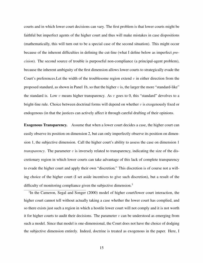
courts and in which lower court decisions can vary. The first problem is that lower courts might be

faithful but imperfect agents of the higher court and thus will make mistakes in case dispositions

(mathematically, this will turn out to be a special case of the second situation). This might occur

because of the inherent difficulties in defining the cut-line (what I define below as imperfect pre-

cision). The second source of trouble is purposeful non-compliance (a principal-agent problem),

because the inherent ambiguity of the first dimension allows lower courts to strategically evade the

Court’s preferences.Let the width of the troublesome region extend v in either direction from the

proposed standard, as shown in Panel 1b, so that the higher v is, the larger the more “standard-like”

the standard is. Low v means higher transparency. As v goes to 0, this “standard” devolves to a

bright-line rule. Choice between doctrinal forms will depend on whether v is exogenously fixed or

endogenous (in that the justices can actively affect it through careful drafting of their opinions.

Exogenous Transparency. Assume that when a lower court decides a case, the higher court can

easily observe its position on dimension 2, but can only imperfectly observe its position on dimen-

sion 1, the subjective dimension. Call the higher court’s ability to assess the case on dimension 1

transparency. The parameter v is inversely related to transparency, indicating the size of the dis-

cretionary region in which lower courts can take advantage of this lack of complete transparency

to evade the higher court and apply their own “discretion.” This discretion is of course not a will-

ing choice of the higher court (I set aside incentives to give such discretion), but a result of the

difficulty of monitoring compliance given the subjective dimension.3

3In the Cameron, Segal and Songer (2000) model of higher court/lower court interaction, the

higher court cannot tell without actually taking a case whether the lower court has complied, and

so there exists just such a region in which a hostile lower court will not comply and it is not worth

it for higher courts to audit their decisions. The parameter v can be understood as emerging from

such a model. Since that model is one-dimensional, the Court does not have the choice of dodging

the subjective dimension entirely. Indeed, doctrine is treated as exogenous in the paper. Here, I

15

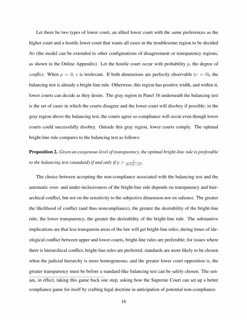
Let there be two types of lower court, an allied lower court with the same preferences as the

higher court and a hostile lower court that wants all cases in the troublesome region to be decided

No (the model can be extended to other configurations of disagreement or transparency regions,

as shown in the Online Appendix). Let the hostile court occur with probability p, the degree of

conflict. When p = 0, v is irrelevant. If both dimensions are perfectly observable (v = 0), the

balancing test is already a bright-line rule. Otherwise, this region has positive width, and within it,

lower courts can decide as they desire. The gray region in Panel 1b underneath the balancing test

is the set of cases in which the courts disagree and the lower court will disobey if possible; in the

gray region above the balancing test, the courts agree so compliance will occur even though lower

courts could successfully disobey. Outside this gray region, lower courts comply. The optimal

bright-line rule compares to the balancing test as follows:

Proposition 2. Given an exogenous level of transparency, the optimal bright-line rule is preferable

to the balancing test (standard) if and only if p > 18v2(2�v)2 .

The choice between accepting the non-compliance associated with the balancing test and the

automatic over- and under-inclusiveness of the bright-line rule depends on transparency and hier-

archical conflict, but not on the sensitivity to the subjective dimension nor on salience. The greater

the likelihood of conflict (and thus noncompliance), the greater the desirability of the bright-line

rule; the lower transparency, the greater the desirability of the bright-line rule. The substantive

implications are that less transparent areas of the law will get bright-line rules; during times of ide-

ological conflict between upper and lower courts, bright-line rules are preferable; for issues where

there is hierarchical conflict, bright-line rules are preferred; standards are more likely to be chosen

when the judicial hierarchy is more homogeneous; and the greater lower court opposition is, the

greater transparency must be before a standard-like balancing test can be safely chosen. The sen-

am, in effect, taking this game back one step, asking how the Supreme Court can set up a better

compliance game for itself by crafting legal doctrine in anticipation of potential non-compliance.

16

sitivity of the balancing test to the subjective dimension and salience are both irrelevant because

they affect equally the losses under the optimal bright-line rule and under the balancing test, so

they drop out of the doctrinal choice calculus, at least when transparency is exogenous.

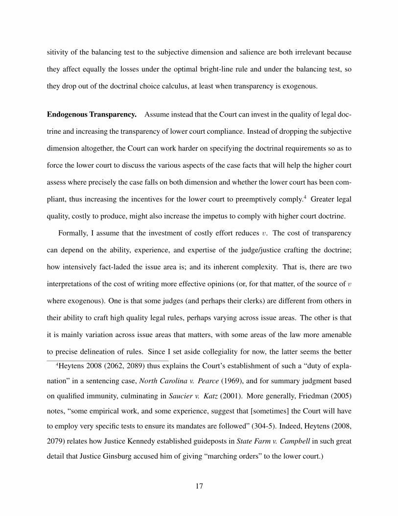
Endogenous Transparency. Assume instead that the Court can invest in the quality of legal doc-

trine and increasing the transparency of lower court compliance. Instead of dropping the subjective

dimension altogether, the Court can work harder on specifying the doctrinal requirements so as to

force the lower court to discuss the various aspects of the case facts that will help the higher court

assess where precisely the case falls on both dimension and whether the lower court has been com-

pliant, thus increasing the incentives for the lower court to preemptively comply.4 Greater legal

quality, costly to produce, might also increase the impetus to comply with higher court doctrine.

Formally, I assume that the investment of costly effort reduces v. The cost of transparency

can depend on the ability, experience, and expertise of the judge/justice crafting the doctrine;

how intensively fact-laded the issue area is; and its inherent complexity. That is, there are two

interpretations of the cost of writing more effective opinions (or, for that matter, of the source of v

where exogenous). One is that some judges (and perhaps their clerks) are different from others in

their ability to craft high quality legal rules, perhaps varying across issue areas. The other is that

it is mainly variation across issue areas that matters, with some areas of the law more amenable

to precise delineation of rules. Since I set aside collegiality for now, the latter seems the better4Heytens 2008 (2062, 2089) thus explains the Court’s establishment of such a “duty of expla-

nation” in a sentencing case, North Carolina v. Pearce (1969), and for summary judgment based

on qualified immunity, culminating in Saucier v. Katz (2001). More generally, Friedman (2005)

notes, “some empirical work, and some experience, suggest that [sometimes] the Court will have

to employ very specific tests to ensure its mandates are followed” (304-5). Indeed, Heytens (2008,

2079) relates how Justice Kennedy established guideposts in State Farm v. Campbell in such great

detail that Justice Ginsburg accused him of giving “marching orders” to the lower court.)

17

interpretation to keep in mind. The formal technology is similar, of course.

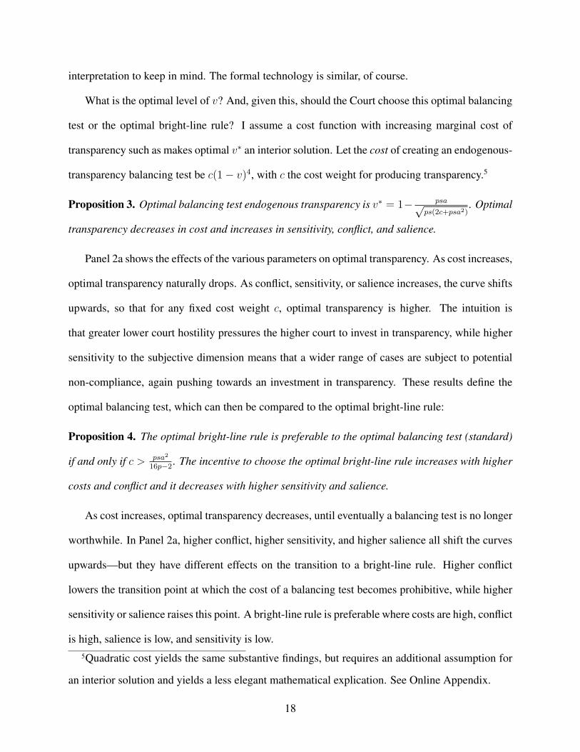
What is the optimal level of v? And, given this, should the Court choose this optimal balancing

test or the optimal bright-line rule? I assume a cost function with increasing marginal cost of

transparency such as makes optimal v⇤ an interior solution. Let the cost of creating an endogenous-

transparency balancing test be c(1� v)4, with c the cost weight for producing transparency.5

Proposition 3. Optimal balancing test endogenous transparency is v⇤ = 1� psapps(2c+psa2)

. Optimal

transparency decreases in cost and increases in sensitivity, conflict, and salience.

Panel 2a shows the effects of the various parameters on optimal transparency. As cost increases,

optimal transparency naturally drops. As conflict, sensitivity, or salience increases, the curve shifts

upwards, so that for any fixed cost weight c, optimal transparency is higher. The intuition is

that greater lower court hostility pressures the higher court to invest in transparency, while higher

sensitivity to the subjective dimension means that a wider range of cases are subject to potential

non-compliance, again pushing towards an investment in transparency. These results define the

optimal balancing test, which can then be compared to the optimal bright-line rule:

Proposition 4. The optimal bright-line rule is preferable to the optimal balancing test (standard)

if and only if c > psa2

16p�2 . The incentive to choose the optimal bright-line rule increases with higher

costs and conflict and it decreases with higher sensitivity and salience.

As cost increases, optimal transparency decreases, until eventually a balancing test is no longer

worthwhile. In Panel 2a, higher conflict, higher sensitivity, and higher salience all shift the curves

upwards—but they have different effects on the transition to a bright-line rule. Higher conflict

lowers the transition point at which the cost of a balancing test becomes prohibitive, while higher

sensitivity or salience raises this point. A bright-line rule is preferable where costs are high, conflict

is high, salience is low, and sensitivity is low.5Quadratic cost yields the same substantive findings, but requires an additional assumption for

an interior solution and yields a less elegant mathematical explication. See Online Appendix.

18

Panel 2b reveals more complicated trade-offs between these parameters in optimal doctrinal

choice. The two panels represent two perspectives on this choice. Each panel considers a pair

of parameters and shows the regions in which a bright-line rule should be chosen as opposed to

choosing the balancing test. A dividing line is shown for higher or lower values of the remaining

parameters. While judges who face higher costs (perhaps due to lower expertise in the issue area

in question or greater legal complexity) will prefer bright-line rules, a greater concern for the first

dimension will push towards a balancing test. When sensitivity is low, it is only those judges who

face low costs or low complexity (given their own ability or the issue area’s features) that will

choose balancing tests. Overall, this suggests that the judges will choose balancing tests (even

when they will be somewhat standard-like) for legal issues in which they have greater expertise or

skill, where they have a greater bank of precedent to draw upon, or where the issue area is more

amenable to delineation. Bright-line rules will make the better tactical choice in more complex or

newer areas of the law, or given dimensions that resist easy quantification.

Discretion and Effort. To what extent will there exist the potential for non-compliance given

optimal doctrinal choice? Or, to put this another way, what degree of discretion will remain after

such choice? Next, what level of effort will be expended given optimal rule choice? The answers

can be derived from Propositions 3 and 4. Define residual discretion d⇤ as the leeway a lower court

will have given optimal rule choice. When a bright-line rule is chosen, it will take the value zero.

When the balancing test is chosen, discretion will take the value v⇤, (that is, it maps to transparency,

which is smaller when the resulting region of potential non-compliance is larger). Effort is the cost

paid by the Court (zero for a bright-line rule). The results are shown in Figure 3. The level of

residual discretion given optimal doctrinal choice depends on the sensitivity of the balancing test,

the costs of reducing discretion, and the degree of conflict between the courts. The most striking

feature of these results is that discretion and cost are non-monotonic, discontinuous functions. For

19

example, as the cost of crafting doctrine increases, discretion given to the lower courts initially in-

creases, because the Court economizes by writing lower quality rules—but eventually, as the costs

continue to rise (say, in highly technical areas where supervision is difficult) the optimal choice

transitions to a bright-line rule, under which some cases are automatically decided incorrectly and

lower court discretion vanishes. Hierarchical conflict reveals a similarly discontinuous effect when

the Court breaks in favor of the bright-line rule, but here the effect of conflict is monotonic. The

sensitivity to the subjective dimension reveals a pattern similar to that for cost, but in the other

direction. As sensitivity increases, there is at first no effect on discretion: the Court will still use

a bright-line rule, until the point at which the balancing test is optimal, but one where the residual

discretion is high. As sensitivity increases further, residual discretion increases then decreases.

Substantively, these formal comparative statics mean that doctrinal choice creates strange bed-

fellows. Low residual discretion is associated with both the lowest-skilled and highest-skilled

justices (those who face, respectively, the highest or lowest costs of generating transparency). The

former choose bright-line rules and thus get full compliance (albeit with a non-ideal doctrine); the

latter will craft high-quality balancing tests that still manage to rein in lower courts to a significant

degree. The same is true for justices with high or low (as opposed to middling) concern for the

substantive dimension—both types yield relatively low levels of residual discretion as compared to

their more moderate brethren (the former invoke good balancing tests; the latter prefer bright-line

rules). Shifted the focus from judicial ability to the nature of the issue area, the simplest and most

complex areas (lowest and highest costs) will be associated with low residual discretion. Finally,

note that increasing the higher court’s resources (or choosing justices with greater legal ability in-

creases higher court control but also can affect doctrinal choice, leading to great use of standards

instead of bright-line rules. More resources will also lead to greater doctrinal complexity.

Higher conflict within the hierarchy should lead to less discretion for lower courts, as the higher

court increasingly turns to bright-line rules or at least invests in more constraining standards (cf.

20

McNollgast 1995, which argues that the Court relaxes its hold when faced with conflict). The

relationship of conflict to doctrinal development is more complicated given the non-monotonic

relationship discussed earlier. We might expect to see the most development not when the lower

courts are so allied with the higher court that specificity is unnecessary, nor when the lower courts

are so hostile that standards are too dangerous, but rather in the middle ground when there are

lower courts to constrain and it is necessary and feasible to do so.

Doctrinal Complexity. Legal complexity has an effect on doctrinal choice, but the incentives

for doctrinal choice also have an effect on legal complexity. The simpler relationship has already

been mentioned, but I highlight it again here. The more complicated the area of the law, the greater

the cost of increasing transparency (if transparency is endogenous) or the lower transparency will

be outright (if transparency is exogenous). Either way, this relationship pushes towards the use

of bright-line rules. On the other hand, where transparency is exogenously high or “cheap” to

produce because the legal issues are more clear-cut, balancing tests can be safely used. Figure 3

shows how complexity is affected given changes in the model parameters. Not all these effects

would be intuitive without the model to guide analysis. For example, for any given cost parameter,

as conflict increases, doctrinal complexity, in the sense of detailed specification, will increase

to better control the lower courts... until it is so costly to do so given rising conflict that the

higher court instead drops down to a straightforward bright-line rule. There is another potential

implication. The results above have been discussed in terms of a choice between a bright-line rule

that simplifies a balancing test from two dimensions back to one dimension. Extending the logic

to multiple dimensions, the same incentives should drive the choice to add a marginal dimension

to any area of the law—at least where that dimension is subjective in nature.

Precision. Setting aside any principal-agent problems, suppose instead that lower courts are

faithful but imperfect agents of the higher court. One can call the degree to which lower courts can

21

apply the higher court doctrine correctly precision. The formal results and most discussion above

can be adjusted to suit this interpretation of the v parameter.6 Thus, the model can speak to both

the “agency” (or principal-agent) perspective on hierarchy, as above, and the “team” perspective,

by recognizing issues of error correction and reduction.

Ideology, Collegiality, and Polarization. Work on judicial choice can conflate what is best for a

given justice with what is best for the Court (Vermuele 2005). So far, I have not considered how the

implications of the model apply differently to individual justices as opposed to the Court. While

full consideration of the complicated relationship between hierarchy and collegiality is beyond

the scope of this paper (see Kastellec 2011, connecting lower court collegiality and hierarchy), I

informally discuss how the model above can improve our understanding of this relationship.

I begin by considering how judicial ideology relates to doctrinal choice. There are actually

two potential relationships. The first is that doctrinal choice corresponds to ideology directly, so

that liberals and conservatives will split over doctrinal form. The more complicated possibility

would be that liberals and conservatives (the extremes) are similar as compared to moderates. For

example, it is argued that more extreme justices such as Scalia tend to prefer bright-line rules

whereas moderates such as O’Connor prefer standards or balancing tests (e.g., Shapiro 2006, 274).

Can this be explained by the incentives shown here? When should we expect “ends-against-the-

middle” doctrinal choice versus more straightforward ideological splits over doctrine?

6One way to do this is to let the probability of correct choice within the v region be p = 12 , so

that both dispositions are equally likely within the imprecise region. Then, if the balancing test

has exogenous precision, the optimal bright-line rule is preferable to the balancing test if and only

if v > 1 �p

4�p2

2 . For exogenous precision, the Court should announce a bright-line rule if it is

sufficiently low. If precision is endogenous, then optimal endogenous precision of the balancing

test occurs at v⇤ = 1 � asps(2c+a2s)

, and the optimal bright-line rule is preferable to the optimal

balancing test (standard) if and only if c > a2s14 . These follow from the proofs for transparency.

22

One possibility is that such justices are so extreme that they already directly prefer a rule of

“always” or of “never.” More moderate justices might still prefer balancing tests, but this makes

the debate rather trivial. The more interesting questions of doctrinal choice arise for those extreme

justices short of such extremes, who might still prefer a balancing test. Assume then that that is

the case. Let them agree on sensitivity (slope) but differ in how high or low the line is drawn

(the intercept). The justices with higher intercepts want more Yes outcomes; those with lower

intercepts/lines want more No outcomes. But they each prefer the same tradeoff between the two

dimensions. In such a configuration, the role of the differing intercept plays a simple role in

doctrinal choice: none, given Proposition 4. All else equal, either they all prefer bright-line rules

(albeit set at a different “height” ), or they all prefer parallel balancing tests (again, set at different

“heights” ). Ideology is then orthogonal to the choice of doctrinal structure.

Suppose that the justices instead vary in terms of sensitivity to the subjective dimension. Then,

we should not find ends-against-the-middle, but rather that those with higher sensitivity prefer bal-

ancing tests (see Figure 2b and Proposition 4). It seems reasonable to suppose that liberalism might

indeed positively correlate with sensitivity to such a dimension (for example, whether exonerating

factors matter for sentencing), but so might conservatism in other areas of the law (the degree to

which good faith exonerates an improper search and seizure). Either way, we would expect a split

along party lines on doctrinal structure.

Recall Figure 3, which shows that high and low levels of sensitivity induce lower levels of

residual discretion than do moderate levels. When ideology correlates with sensitivity, this sug-

gests that liberals and conservatives would both leave less discretion in the hands of the lower court

than moderates: one wing because it would choose a bright-line rule, the other because it would

construct a high-quality balancing test. The point remains, however, that it is not extremism in

terms of the absolute number of “yes” or “no” dispositions that directly affects optimal doctrinal

form, but rather sensitivity to the subjective dimension. Note also that the effects of sensitivity

23

depend on the justices having influence over transparency—if they do not, then we return to the

solution for exogenous transparency and Proposition 2, in which sensitivity to the subjective di-

mension does not affect doctrinal choice even if sensitivity does vary by ideology.

There are two further wrinkles to the ideology/doctrine debate, as two other parameters shown

to affect the justices’ incentives might vary with ideology: salience and conflict. Salience might

vary with ideology because the distribution of cases in the case space might vary. That is, there

might be many more cases falling in the middle of the case space than at the extremes. The trou-

blesome region might capture a greater number of potential lower court cases when it is in the

moderate region of the case space than when it lies near one extreme or the other. The set of cases

for which transparency might create a problem would then be much smaller for Scalia’s preferred

balancing test, which would lie much higher in the case space than for Kennedy’s preferred balanc-

ing test. In the formal model, this is easily captured by the salience weight for this issue—Scalia

would have to worry less about this region than Kennedy and so s would be lower for Scalia than

for Kennedy. If transparency is exogenous, this is irrelevant, as salience is irrelevant for choice. If

transparency is endogenous, then higher salience suggests a balancing test so that moderate justices

would indeed be more likely to prefer the balancing test over the bright-line rule relative.

Next, when justices are more extreme, they are likely to be positioned differently with respect

to lower courts than are moderate justices. Much depends on the distribution of lower court judges.

Suppose that, as might seem likely, the lower courts are roughly distributed around the center of

the Supreme Court, and that the distribution of lower courts follows a bell curve, with many more

lower courts concentrated near the center of the higher court with fewer in the wings. If that is

the case, then a more extreme justice will find few allies in the courts below, and a more moderate

justice will find it far more likely that a random lower court will resemble her own preferences

for case dispositions. This suggests that, all else equal, moderate justices face a lower likelihood

of a hostile lower court (lower p) than a more extreme justice. In turn, this means that, if the

24

concentration of lower courts is sufficiently high, then moderate justices should prefer balancing

tests and more extreme justices should prefer bright-line rules (see Figure 2b). The intuition is that

O’Connor is less worried about lower court discretion since she has a greater expectation they will

decide as she would anyway. Scalia will find fewer allies below and so will do better accepting the

losses of a bright-line rule than using a balancing test. The salience argument and the compliance

argument are mutually reinforcing, in that both suggest moderates will be more likely to prefer

balancing tests than will more extreme justices. The patterns of discretion, however, would be less

clear-cut: discretion is monotonic with respect to conflict but not to salience.

These arguments can be extended to consider how polarization might affect doctrinal outputs.

A Court full of moderate justices would tend to produce a greater number of balancing tests, all

else equal. But, in a polarized Court, with relatively extreme justices on both sides, each side

would prefer bright-line rules. Indeed, even if only one wing of the Court is extreme, if it has the

majority, it would be more likely to produce bright-line rules.

However, one further complication is the varying perspectives of opinion authors versus other

members of the majority (see, e.g., Heytens 2008, 2092 on the split over the granting of discretion

in summary judgment-qualified immunity cases, in Crawford-El v. Britton (1998)). When we say

that Justice Scalia prefers bright-line rules and Justice O’Connor prefers balancing tests, do we

mean that those choices represent what each would choose were he or she dictator? Or that Justice

Scalia wants Justice O’Connor’s preferred balancing test to be converted into the nearest bright-

line rule? Such a bright-line rule would obviously differ from Scalia’s preferred bright-line rule.

That is, is he disagreeing with her incorporation of the subjective dimension or the placement of

the rule in the case space? Does he simply want a more extreme test or one that rejects one of the

constituent dimensions of the rule?

Note that a more extreme justice, say more conservative than the author, might actually like

some non-compliance from conservative lower courts. Such a justice might prefer a foggier stan-

25

dard, then, depending on how the lower courts are configured vis-a-vis the higher court and the

standard in question. For that matter, say there is a justice sufficiently extreme so as to be higher

than the troublesome region of a bright-line rule as shown in Figure 1, Panel 1a. The most extreme

justice would be one who prefers the entire speed case space to be treated as Y es. Suppose he has

to choose between the bright-line rule as shown and the balancing test as shown, both for a more

moderate opinion author. While the author would prefer the balancing test representing her true

preferences to be enacted, the extreme justice will be indifferent between the bright-line rule and

the balancing test: The shaded triangle on the left would now be handled correctly (Y es) accord-

ing to the extreme justice’s own preferred rule at the expense of the shaded triangle on the right,

which is now incorrectly decided (No) but these two triangles are of equal area.7 (For the author,

both these triangles now have wrong dispositions.) Similarly, to extend the polarization argument

above, while each wing may prefer its own bright-line rule to a moderate justice’s preferred stan-

dard, these will differ, with the liberal one being “high” and the conservative one ”low” (or vice

versa)—and each wing might prefer the moderate standard to the “wrong” bright-line rule.

Moreover, suppose that the production of legal quality (transparency) is in the hands of the

opinion author. The optimal choice of doctrinal form can depend on who exactly is crafting the

doctrine. It could be largely the author’s ability that matters—so that Justice Scalia might prefer a

balancing test if he himself were crafting it, but might prefer a bright-line rule if Justice Kennedy is

to craft it. Or, since it is the opinion author that must bear the costs of authorship, one justice might

want another to invest in a balancing test when he himself would simply go with the cheaper bright-

line rule. There is also the burden of authorship to be taken into account. As shown in Lax and

Cameron (2007), the most preferred opinion can vary depending on whether a justice personally7Equal impact only holds under the area-utility assumption; if the extreme justice cared more

about the righthand triangle because those cases are further away from his preferred rule along the

top of the square, then the bright-line rule would actually be better.

26

has to pay the cost of crafting the rule or whether another justice will. Justice A can want Justice

B to shrink the non-compliance region under a standard to zero by investing in opinion quality, but

Justice A might not be willing to invest the required amount of effort himself or herself.8

Another question is what will happen in the end if justices do prefer different doctrines. One

treatment of this is Lax (2007) showing that a median rule exists even when there is not a single

median justice: there is an “implicit median rule” that is the baseline prediction, so that collegiality

alone is shown to be insufficient for non-“median” outcomes. (Institutional features and incentives

also affect collegial rule construction). For now, note that where the justices agree about the slope

but not the intercept of the balancing test, the implicit median rule would also be a balancing test

with that slope and the median intercept. Where they agree on the intercept and not the slope, the

implicit median rule would have that intercept and the median slope. Where there is more compli-

cated variation, the implicit median rule can take a very different structural form, and, as shown

in Lax (2007) need not be a straightforward balancing test. Connecting that paper (wherein the

issues of hierarchy-based incentives rule choice are set aside except for a result on enforceability)

with this paper (which focuses on those very incentives), extending and integrating both lines of

analysis, is a natural next step in this research. For now, this informal discussion sketches some

intriguing aspects of the collegiality-hierarchy intersection, suggesting that this type of modeling,

focusing on the judicial politics of legal doctrine, provides a promising way to move forward. It

also demonstrates how much more complicated judicial choice can be than some accounts suggest.

Conclusion

The primary debate in judicial politics is whether judicial decisions depend on more than legal

precedents, principles, and text—and whether and how external, collegial, or hierarchical politics

shape law. I have argued that justices (or other appellate judges) concerned about the impact of8A justice might, of course, assist with such efforts with suggestions and comments—what is

often seen as bargaining at the expense of the author could work to his/her benefit.

27

their opinions on future case outcomes are indeed constrained in their choices, and I have shown

that the separation of rule creation and rule application creates striking incentives for the former.

In short, hierarchical politics do shape law.

Moreover, while Court observers often attribute judicial use of different types of rules to id-

iosyncratic preference, I show that there are clear incentives for rule choice, providing micro-

foundations for the variation therein. The model captures some of the fundamental tensions driving

doctrinal choice, specifically the choice between bright-line rules and standards. The resolution of

these tensions depends in a nuanced way on the degree of lower court conflict, the salience of the

issue, the complexity of that issue, the expertise and abilities of the rule crafter, the sensitivity

of the preferred doctrine to varying case facts, and the nature of the doctrine’s constituent factual

dimensions. These factors can induce insincere doctrinal choice and affect the care taken in craft-

ing legal doctrine, that is, the investment in legal “quality.” Doctrinal choice, doctrinal complexity,

lower court discretion, and the allocation of judicial resources to an area of the law are all shown

to be affected by hierarchical politics (thus connecting hierarchical politics to the rule of law).

The model suggests that our understanding of how ideology impacts the law may be incomplete

or naive, because intra-Court collegial politics may be connected in striking ways to hierarchical

politics. A justice’s underlying liberalism or conservatism can lead to nonintuitive incentives for

doctrinal choice. These incentives create odd patterns of ideological and doctrinal alignment, with

strange bedfellows on both wings of the court opposing the middle. Some may find it disconcerting

for the rule of law that the selection of winners and losers can depend on how liberal or conserva-

tive a given Supreme Court justice is. It is even more disconcerting that doctrine can depend on

judicial strategy. While disagreement on the bench can sometimes be attributed to sincere beliefs

in different legal philosophies rather than crude ideological differences, strategic incentives that

undercut such sincere choices undermine even that defense.

Future work might extend the model to explore other contexts. The rules/standards model

28

shares some insights with the traditional delegation literature, which tends to focus on congres-

sional and bureaucratic institutions (e.g., Kiewiet and McCubbins 1991; Epstein and OHalloran

1999). For example, the connection between doctrinal choice and intra-hierarchy conflict resem-

bles the “ally principle” in standard delegation models (one gives more discretion to those with

similar preferences). These analogies might be explored, applying the rules/standards model to

those contexts to the extent that legislatures and bureaucracies also enact preferences by construct-

ing rules for dividing up the space of possible actions into permissible and impermissible. Within

the judicial context, more work could be done on collegiality and other types of hierarchical con-

flict. One could also explore how transparency and legal quality are achieved.

While this paper is theoretical, it also suggests we need to seek new ways to measure legal

preferences and output empirically, going beyond unidimensional policy points or the percent of

votes cast in the liberal direction, and even beyond recent advances in the ideological location of

opinions. Possibilities include “classification trees” (Kastellec 2010) or making use of advances in

computerized textual analysis. Moreover, much as Staton and Vanberg (2008) argue that strategic

vagueness can undercut straightforward separation-of-powers tests, ignoring strategic incentives

for doctrinal choice can undercut straightforward assessments of judicial ideology, as well as of

lower court compliance and discretion.

Formal Appendix

The variables in the formal model are: a – sensitivity to the subjective factual dimension (the

slope parameter, capturing the trade-off between the two dimensions); b – the intercept of the rule

with the axis; s – salience of the issue area; v – lack of transparency (higher values mean a wider

troublesome range, this can be exogenous or endogenous; p – likelihood of a hostile lower court; c

– cost weight for producing transparency; aL – sensitivity for the lower court when hostile; and bL

– intercept for the lower court when hostile. I assume that for any value of x, there is some value

29

of y that yields a Yes disposition, which requires b 1 and 0 a b (yielding the configuration

shown in Figure 1. For constraining the lower court to be outside the troublesome region in the

exogenous transparency solution, it suffices to assume that bL b � av and aL � a�(b�bL)1�v . For

the endogenous transparency solution, this would invoke v⇤, which is implicitly defined.

Proof of Prop. 1. If y is set above the upper limits or below the lower limits of y, then the full re-

gion of area a2 is lost (payoff u = �sa2

4 ). Otherwise, the area is 12(b�y)

�b�ya

�+1

2

�1� b�y

a

�(y � (b� a)).

Utility is then u =�⇣(a2�2a(b�y)+2(b�y)2)

2s⌘

4a2 with @u@y =

�((2a�4(b�y))(a2�2a(b�y)+2(b�y)2)s)2a2 with

maximum at y⇤ = b� a2 (payoff u⇤ = �sa2

16 ). The combined area of the loss region is a4 .

Proof of Prop. 2. The troublesome region area is a(2v�v2) (half is in contention). The rule payoff

is greater than the balancing payoff⇣�1

2spa2 (2v � v2)2

⌘if p > 1

8v2(2�v)2 .

Proof of Prop. 3. The balancing test payoff is �12ps(a(2v � v2))2 � c(1 � v)4, so that @u

@v =

�4 (�1 + v)�c(�1 + v)2 + 1

2a2ps (�2 + v) v

�which is zero at v⇤ = 1 � psap

ps(2c+psa2)(unique

for interior v⇤). The second derivative is @2u@v2 = �4

�3c(�1 + v)2 + 1

2a2ps (2 + 3 (�2 + v) v)

�,

which at v⇤ is �4pa2, which is negative making v⇤ a maximum. Comparative statics follow

from the partial derivatives and can be signed as follows: @v⇤

@a = �✓2cq

ps(2c+psa2)3

◆< 0;

@v⇤

@p = �2acq

sp(2c+psa2)3

< 0; @v⇤

@s = �acq

ps(2c+psa2)3

< 0; and @v⇤

@c = as2p2

(sp(2c+spa2))32> 0.

Proof of Prop. 4. The bright-line rule payoff⇣

�sa2

16

⌘is greater than that of the standard

⇣�cpsa2

2c+spa2

⌘

when c+ psa2

2 < 8cp. If p < 18 , then this cannot occur for positive values of the parameters, but oth-

erwise it holds when c > psa2

16p�2 . If c is higher, the condition is directly easier to satisfy. Otherwise,

the partial derivative of the right-hand side of the condition on cost gives the comparative statics:

@@a = spa

8p�1 > 0, @@p = �sa2

(8p�1)2 < 0, and @@s = pa2

16p�2 > 0. The boundary on c for a bright-line rule is

thus higher for higher a or s, or lower p, each of which make the balancing test more attractive.

ReferencesCameron, Charles M. 1993. “New Avenues for Modeling Judicial Politics.” Prepared for delivery

at the Conference on the Political Economy of Public Law, Rochester, N.Y.

30

Cameron, Charles M., Jeffrey A. Segal and Donald R. Songer. 2000. “Strategic Auditing in a Politi-

cal Hierarchy: An Informational Model of the Supreme Court’s Certiorari Decisions.” American

Political Science Review 94:101–16.

Epstein, David and Sharyn OHalloran. 1999. Delegating Powers: A Transaction Cost Politics

Approach to Policy Making under Separate Powers. Cambridge: Cambridge University Press.

Fallon, Richard H. 2001. Implementing the Constitution. Cambridge, MA: Harvard University

Press.

Friedman, Barry. 2005. “The Politics of Judicial Review.” Texas Law Review 84:257–337.

Grofman, Bernard. 1993. “Public Choice, Civic Republicanism, and American Politics: Perspec-

tives of a ‘Reasonable Choice’ Modeler.” Texas Law Review 71:1541–1587.

Heytens, Toby J. 2008. “Doctrine Formulation and Distrust.” Notre Dame Law Review 83:2045.

Jacobi, Tonja and Emerson H. Tiller. 2007. “Legal Doctrine and Political Control.” Journal of Law,

Economics, & Organization 23(2):326–45.

Kaplow, Louis. 1992. “Rules versus Standards: An Economic Analysis.” Duke Law Journal

42(3):557–629.

Kastellec, Jonathan P. 2007. “Panel Composition and Judicial Compliance on the United States

Courts of Appeals.” Journal of Law, Economics & Organization 23(2):421–41.

Kastellec, Jonathan P. 2010. “The Statistical Analysis of Judicial Decisions and Legal Rules with

Classification Trees.” Journal of Empirical Legal Studies 7(2):202–30.

Kastellec, Jonathan P. 2011. “Hierarchical and Collegial Politics on the U.S. Courts of Appeals.”

Journal of Politics Forthcoming.

Kiewiet, Roderick and Mathew McCubbins. 1991. The Logic of Delegation: Congressional Parties

and the Appropriation Process. Chicago: University of Chicago Press.

Kornhauser, Lewis. A. 1992a. “Modeling Collegial Courts I: Path Dependence.” International

Review of Law and Economics 12:169–85.

Kornhauser, Lewis A. 1992b. “Modeling Collegial Courts II: Legal Doctrine.” Journal of Law

Economics & Organization 8:441–70.

31

Landa, Dimitri and Jeffrey R. Lax. 2008. “Disagreements on Collegial Courts: A Case-Space

Approach.” Journal of Constitutional Law 10(2):305–29.

Landa, Dimitri and Jeffrey R. Lax. 2009. “Legal Doctrine in Collegial Courts.” Journal of Politics

71(3).

Lax, Jeffrey R. 2003. “Certiorari and Compliance in the Judicial Hierarchy: Discretion, Reputa-

tion, and the Rule of Four.” Journal of Theoretical Politics 15(1):61–86.

Lax, Jeffrey R. 2007. “Constructing Legal Rules on Appellate Courts.” American Political Science

Review. 101(3):591–604.

Lax, Jeffrey R. 2011. “The New Judicial Politics of Legal Doctrine.” Annual Review of Political

Science 14:131–57.

Lax, Jeffrey R. and Charles M. Cameron. 2007. “Bargaining and Opinion Assignment on the U.S.

Supreme Court.” Journal of Law, Economics, and Organization 23(2):276–302.

McNollgast. 1995. “Politics and the Courts: A Positive Theory of Judicial Doctrine and the Rule

of Law.” Southern California Law Review 68:1631–89.

Segal, Jeffrey A. and Harold J Spaeth. 2002. The Supreme Court and the Attitudinal Model Revis-

ited. New York: Cambridge University Press.

Shapiro, Carolyn. 2006. “The Limits of the Olympian Court: Common Law Judging versus Error

Correction in the Supreme Court.” Washington and Lee Law Review 63:271–337.

Staton, Jeffrey K. and Georg Vanberg. 2008. “The Value of Vagueness: Delegation, Defiance, and

Judicial Opinions.” American Journal of Political Science 52(3):504–19.

Sullivan, Kathleen M. and Akhil Reed Amar. 1992. “The Supreme Court, 1991 Term.” Harvard

Law Review 106(1):19–122.

Tiller, Emerson H. and Frank B. Cross. 2006. “What is Legal Doctrine?” Northwestern University

Law Review 100(1):517–34.

Vermuele, Adrian. 2005. “The Judiciary is a They, Not an It: Interpretive Theory and the Fallacy

of Division.” Journal of Contemporary Legal Issues 14:549–84.

32

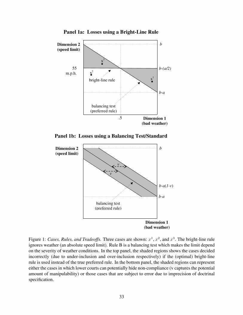
Panel 1a: Losses using a Bright-Line Rule

Panel 1b: Losses using a Balancing Test/Standard

The bright-line rule ignores weather (an absolute speed limit). Rule B is a balancing test which makes the limit depend on the severity of weather conditions. In the top panel, the shaded regions shows the cases decided incorrectly (due to under-inclusion and over-inclusion respectively) if the (optimal) bright-line rule is used instead of the true preferred rule. In the bottom panel, the shaded regions can represent either the cases in which lower courts can potentially hide non-compliance (v captures the potential amount of manipulability) or those cases that are subject to error due to imprecision of doctrinal specification.

Dimension 1 (bad weather)

balancing test (preferred rule)

b

b-a

Dimension 2 (speed limit)

v

v

b-a(1-v)

Dimension 1 (bad weather)

55 m.p.h.

b

b-(a/2)

b-a

Dimension 2 (speed limit)

.5

bright-line rule

balancing test (preferred rule)

.

. .

x3

x1

x2

Figure 1: Cases, Rules, and Tradeoffs. Three cases are shown: x1, x2, and x3. The bright-line ruleignores weather (an absolute speed limit). Rule B is a balancing test which makes the limit dependon the severity of weather conditions. In the top panel, the shaded regions shows the cases decidedincorrectly (due to under-inclusion and over-inclusion respectively) if the (optimal) bright-linerule is used instead of the true preferred rule. In the bottom panel, the shaded regions can representeither the cases in which lower courts can potentially hide non-compliance (v captures the potentialamount of manipulability) or those cases that are subject to error due to imprecision of doctrinalspecification.

33

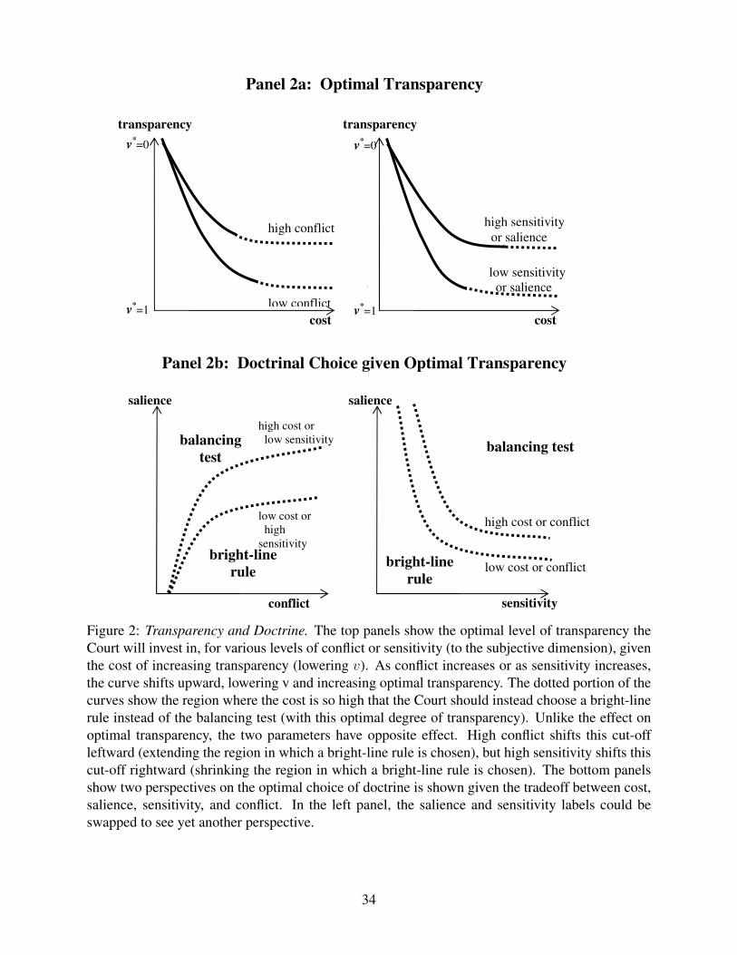
Panel 2a: Optimal Transparency

Panel 2b: Doctrinal Choice given Optimal Transparency

The top panels show the optimal level of transparency the Court will invest in, for various levels of conflict or sensitivity (to the subjective dimension), given the cost of increasing transparency (lowering v). As conflict increases or as sensitivity increases, the curve shifts upward, lowering v and increasing optimal transparency. The dotted portion of the curves show the region where the cost is so high that the Court should instead choose a bright-line rule instead of the balancing test (with this optimal degree of transparency). Unlike the effect on optimal transparency, the two parameters have opposite effect High conflict shifts this cut-off leftward (extending the region in which a bright-line rule is chosen), but high sensitivity shifts this cut-off rightward (shrinking the region in which a bright-line rule is chosen). The bottom panels show two perspectives on the optimal choice of doctrine is shown given the tradeoff between cost, salience, sensitivity, and conflict. In the left panel, the salience and sensitivity labels could be swapped to see yet another perspective.

v*=0

v*

=1

high conflict

low conflict

transparency

cost

high sensitivity or salience

transparency

v*=0

v*

=1 cost

low sensitivity or salience

bright-line rule

balancing test

high cost or low sensitivity

low cost or high sensitivity

salience

conflict

balancing test

bright-line rule

high cost or conflict low cost or conflict

salience

sensitivity

Figure 2: Transparency and Doctrine. The top panels show the optimal level of transparency theCourt will invest in, for various levels of conflict or sensitivity (to the subjective dimension), giventhe cost of increasing transparency (lowering v). As conflict increases or as sensitivity increases,the curve shifts upward, lowering v and increasing optimal transparency. The dotted portion of thecurves show the region where the cost is so high that the Court should instead choose a bright-linerule instead of the balancing test (with this optimal degree of transparency). Unlike the effect onoptimal transparency, the two parameters have opposite effect. High conflict shifts this cut-offleftward (extending the region in which a bright-line rule is chosen), but high sensitivity shifts thiscut-off rightward (shrinking the region in which a bright-line rule is chosen). The bottom panelsshow two perspectives on the optimal choice of doctrine is shown given the tradeoff between cost,salience, sensitivity, and conflict. In the left panel, the salience and sensitivity labels could beswapped to see yet another perspective.

34

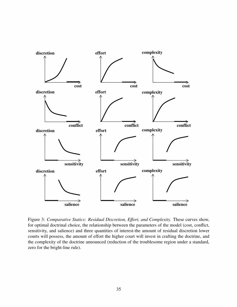
Figure 3: Comparative Statics--Residual Discretion, Effort, and Complexity

These curves show, for optimal doctrinal choice, the relationship between the parameters of the model (cost, conflict, sensitivity, and salience) and three quantities of interest—the amount of residual discretion lower courts will possess, the amount of effort the higher court will invest in crafting the doctrine, and the complexity of the doctrine announced (reduction of the troublesome region under a standard, zero for the bright-line rule).

conflict

discretion

conflict discretion

sensitivity

sensitivity

effort

effort

cost

effort discretion

cost

discretion

salience

salience

effort

conflict

sensitivity

cost

complexity

salience

complexity

complexity

complexity

Figure 3: Comparative Statics: Residual Discretion, Effort, and Complexity. These curves show,for optimal doctrinal choice, the relationship between the parameters of the model (cost, conflict,sensitivity, and salience) and three quantities of interest-the amount of residual discretion lowercourts will possess, the amount of effort the higher court will invest in crafting the doctrine, andthe complexity of the doctrine announced (reduction of the troublesome region under a standard,zero for the bright-line rule).

35

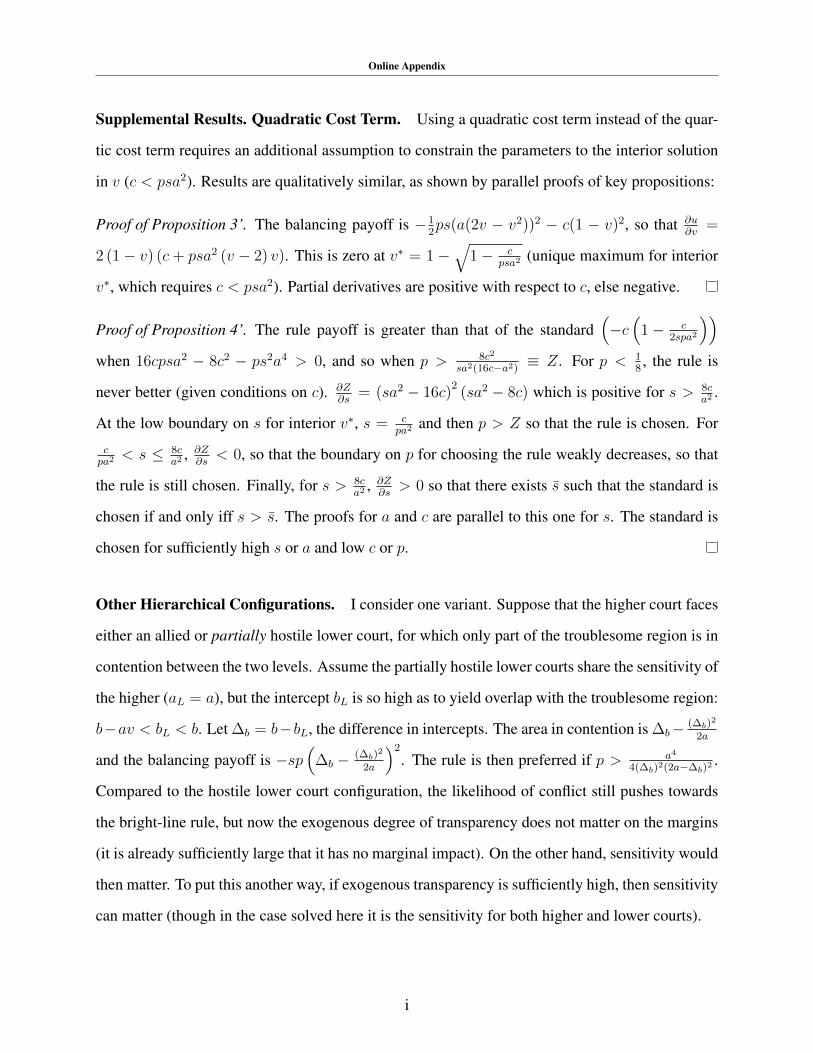
Online Appendix

Supplemental Results. Quadratic Cost Term. Using a quadratic cost term instead of the quar-

tic cost term requires an additional assumption to constrain the parameters to the interior solution

in v (c < psa

2). Results are qualitatively similar, as shown by parallel proofs of key propositions:

Proof of Proposition 3’. The balancing payoff is �12ps(a(2v � v

2))2 � c(1 � v)2, so that @u

@v

=

2 (1� v) (c+ psa

2 (v � 2) v). This is zero at v⇤ = 1 �q

1� c

psa

2 (unique maximum for interior

v

⇤, which requires c < psa

2). Partial derivatives are positive with respect to c, else negative.

Proof of Proposition 4’. The rule payoff is greater than that of the standard⇣�c

⇣1� c

2spa2

⌘⌘

when 16cpsa2 � 8c2 � ps

2a

4> 0, and so when p >

8c2

sa

2(16c�a

2) ⌘ Z. For p <

18 , the rule is

never better (given conditions on c). @Z

@s

= (sa2 � 16c)2 (sa2 � 8c) which is positive for s >

8ca

2 .

At the low boundary on s for interior v⇤, s = c

pa

2 and then p > Z so that the rule is chosen. For

c

pa

2 < s 8ca

2 , @Z

@s

< 0, so that the boundary on p for choosing the rule weakly decreases, so that

the rule is still chosen. Finally, for s >

8ca

2 , @Z

@s

> 0 so that there exists s such that the standard is

chosen if and only iff s > s. The proofs for a and c are parallel to this one for s. The standard is

chosen for sufficiently high s or a and low c or p.

Other Hierarchical Configurations. I consider one variant. Suppose that the higher court faces

either an allied or partially hostile lower court, for which only part of the troublesome region is in

contention between the two levels. Assume the partially hostile lower courts share the sensitivity of

the higher (aL

= a), but the intercept bL

is so high as to yield overlap with the troublesome region:

b�av < b

L

< b. Let �b

= b�b

L

, the difference in intercepts. The area in contention is �b

� (�b)2

2a

and the balancing payoff is �sp

⇣�

b

� (�b)2

2a

⌘2. The rule is then preferred if p >

a

4

4(�b)2(2a��b)2.

Compared to the hostile lower court configuration, the likelihood of conflict still pushes towards

the bright-line rule, but now the exogenous degree of transparency does not matter on the margins

(it is already sufficiently large that it has no marginal impact). On the other hand, sensitivity would

then matter. To put this another way, if exogenous transparency is sufficiently high, then sensitivity

can matter (though in the case solved here it is the sensitivity for both higher and lower courts).

i

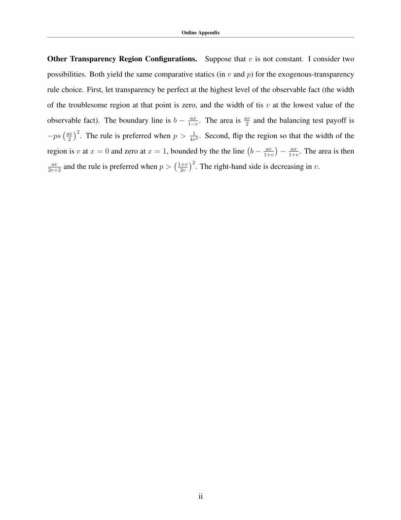
Online Appendix

Other Transparency Region Configurations. Suppose that v is not constant. I consider two

possibilities. Both yield the same comparative statics (in v and p) for the exogenous-transparency

rule choice. First, let transparency be perfect at the highest level of the observable fact (the width

of the troublesome region at that point is zero, and the width of tis v at the lowest value of the

observable fact). The boundary line is b � ax

1�v

. The area is av

2 and the balancing test payoff is

�ps

�av

2

�2. The rule is preferred when p >

14v2 . Second, flip the region so that the width of the

region is v at x = 0 and zero at x = 1, bounded by the the line�b� av

1+v

�� ax

1+v

. The area is then

av

2v+2 and the rule is preferred when p >

�1+v

2v

�2. The right-hand side is decreasing in v.

ii