Embed Size (px)
Citation preview
This document is downloaded from DR‑NTU (https://dr.ntu.edu.sg)Nanyang Technological University, Singapore.
Political corruption and corporate earningsmanagement
Zhang, Jin
2017
Zhang, J. (2017). Political corruption and corporate earnings management. Doctoral thesis,Nanyang Technological University, Singapore.
http://hdl.handle.net/10356/72893
https://doi.org/10.32657/10356/72893
Downloaded on 29 Jan 2022 17:47:12 SGT

POLITICAL CORRUPTION AND CORPORATE EARNINGS MANAGEMENT
ZHANG JIN
NANYANG BUSINESS SCHOOL
2017

POLITICAL CORRUPTION AND CORPORATE EARNINGS MANAGEMENT
ZHANG JIN
NANYANG BUSINESS SCHOOL
A thesis submitted to Nanyang Technological University in partial fulfillment of the
requirements for the degree of Doctor of Philosophy
2017

Acknowledgement
First and foremost, I would like to express my sincere gratitude towards my thesis advisor
Prof. Huai Zhang, for his continuous support during my PhD study. His wisdom, knowledge,
and commitment to high-quality research guide me through this progressive and stimulating
journey. He helps me prepare for an academic career by improving my research capacity,
communication skills, and teaching ability.
I am also deeply grateful for my thesis committee and oral defense committee members:
Prof. Huasheng Gao, Prof. Yen Hee Tong, Prof. Kevin Koh, and Prof. Yachang Zeng, for
their insightful comments and invaluable suggestions. I also want to thank Prof. Rui Shen,
Prof. Terence Ng, Prof. Huaxiang Yin, Prof. Hun-Tong Tan, and other faculty members, for
their sharp and helpful comments in my brownbag seminar.
Special thanks go to my co-authors: Prof. Po-Hsuan Hsu and Prof. Kai Li, for guiding me
to be an academic writer, a professional presenter and a collegiate scholar.
My appreciation also extends to my office colleagues: Mr. Lukas Helikum, Mr Truc
Thuc Do, Mr. Kenny Phua, Ms. Xiaoran Huang, Mr. Chongwu Xia, Mr Tongrui Cao and Mr.
Pingyi Lou. I truly benefit a lot from their advice, encouragement, information sharing, and
technical assistance.
I am also grateful for the help from the admin staff at Nanyang Business School: Ms.
Adeline Tang, Ms. Bee Hua Quek, Ms. Karen Barlaan, and Ms. Tsai Ting Hu. Thank you for
being there and always ready to help.
Last but not the least, I want to thank my family for their love and consistent support
throughout my life.

Contents Abstract ............................................................................................................................... 1
1. Introduction ..................................................................................................................... 2
2. Literature Review and Hypothesis Development ............................................................ 8
3. Research Design ............................................................................................................ 10
3.1 Baseline Model ........................................................................................................ 10
3.2 Measure of Earnings Management .......................................................................... 11
3.3 Measure of Political Corruption .............................................................................. 12
3.4 Control variables ..................................................................................................... 13
4. Sample Formation and Descriptive Statistics ............................................................... 15
4.1 Sample Formation ................................................................................................... 15
4.2 Descriptive Statistics ............................................................................................... 16
5. Empirical Results .......................................................................................................... 18
5.1 Baseline Regression ................................................................................................ 18
5.2 Subsample Analyses ................................................................................................ 19
5.2.1 Geographic Concentration ................................................................................ 19
5.2.2 Political Connections ........................................................................................ 20
5.2.3 Costs of Downward Earnings Management ..................................................... 21
6. Robustness checks ........................................................................................................ 22
6.1 Alternative Measures of Corruption ........................................................................ 22
6.1.1 Alternative Measures Based on Corruption Convictions ................................. 22
6.1.2 Alternative Measures Based on Perception ...................................................... 23
6.2 Restatement Analysis .............................................................................................. 24
6.3 Accounting Policy Analysis .................................................................................... 25
6.4 Instrument Variable Approach ................................................................................ 27
6.5 Difference-in-Differences Analysis ........................................................................ 28
6.6 Tax Avoidance Analysis ......................................................................................... 29
6.7 Party Affiliation ....................................................................................................... 30
6.8 High-Profile Political Corruption Case and Earnings Management ....................... 30
7. Conclusion .................................................................................................................... 32
Reference ........................................................................................................................... 35
Appendix A Variable Definition ....................................................................................... 40
Appendix B Summary Statistics for Corruption by State ................................................. 42

Appendix C Gravity-based Centered Index for Spatial Concentration (GCISC2) ........... 44
Appendix D High-Profile Political Corruption Case and Earnings Management............. 45
Figure 1 Map of the State Average Corruption ................................................................. 47
Table 1 Descriptive Statistics ............................................................................................ 48
Table 2 Baseline Regression ............................................................................................. 50
Table 3 Geographic Concentration ................................................................................... 52
Table 4 Political Connection ............................................................................................. 54
Table 5 Costs of Downward Earnings Management ......................................................... 56
Table 6 Alternative Measures of Corruption ..................................................................... 58
Table 7 Restatement Likelihood ....................................................................................... 61
Table 8 Accounting Policy Analysis ................................................................................. 62
Table 9 Instrument Variable Approach Based on Population Concentration ................... 64
Table 10 Difference-in-Differences Analyses Based on Re-Location .............................. 66
Table 11 Tax Avoidance ................................................................................................... 68
Table 12 State Party Affiliation ........................................................................................ 70

1
Abstract
Using U.S. Department of Justice data on political corruption convictions, I examine how
political corruption affects firms’ earnings management. I find that companies headquartered
in more corrupt states manipulate earnings downwards. The findings are robust to six
alternative corruption measures, the restatement analysis, the accounting policy analysis, the
instrumental variable approach, the difference-in-differences analysis, and an event study. In
addition, I find that the effect of corruption on earnings management is more pronounced for
firms whose operations concentrate in their headquarter states and for firms without political
connections, but is not significant for firms on the edge of missing earnings benchmarks or
firms facing tight debt covenants. In sum, my findings suggest that firms respond to
corruption by managing earnings downwards.
Keywords: Earnings Management, Political Corruption, Rent Seeking
JEL Classification: M41; G38

2
1. Introduction
Political corruption is pervasive and the U.S. is not immune to this problem. In its 2012
Global State of Mind Report, Gallup reports that the percentage of adults who perceive
corruption as a widespread problem in their government is greater than 50%, for 108 out of
129 countries. The percentage for the U.S. stands at 73%1. Consistent with these statistics,
there are plenty of anecdotal evidence of political corruption in the U.S. For example, Don
Siegelman, the former Alabama governor, appointed the CEO of HealthSouth to a state
regulatory board after taking a bribe of $500,000. For another example, several officials of
the Defense Logistics Agency awarded government contracts to United Logistic in exchange
for $800,000.
How does political corruption affect firms’ accounting choices? Given the pervasiveness
of political corruption, this is an important question that has implications for academics,
regulators and the public. However, this question has received scant attention from prior
literature, and I attempt to address this gap.
Following Butler et al. (2009), I define political corruption as agency issues between
elected or appointed government officials and their constituents, which manifest in rent-
seeking by government officials. Public officials can extract rents from firms through the
threat of additional regulations and targeted taxation (McChesney, 1987). According to the
positive accounting theory (Watts and Zimmerman, 1986), downward earnings management
weakens the argument for such government actions, and shields firms from the rent-seeking
of corrupt officials. Besides, if corrupt officials directly solicit bribes, the amount of bribe is
subject to a firm’s profitability (Svensson, 2003). Therefore, I hypothesize that firms facing
high corruption are incentivized to manipulate earnings downwards.
1
The report is available at http://www.gallup.com/file/poll/165497/GlobalStateMind_Report_10-
13_mh.pdf.

3
This hypothesis is not without tension. Numerous studies have shown that political favors
increase firm value (Fisman, 2001; Faccio et al., 2006; Claessens et al., 2008; Goldman, et al.,
2009; Duchin and Sosyura, 2012; Tahoun, 2014), and corruption offers opportunities for
firms to bribe their way into an advantageous position. Expenses related to illicit dealings
with government officials are likely hidden from the public (Gul, 2006). Since these expenses
can’t be reasonably expected by investors, they are likely to result in actual earnings falling
short of the market’s expectation. To avoid these negative surprises, firms have incentives to
manipulate earnings upwards.
Using a sample of 56,096 observations, I take the question to the data. To measure
corruption, I follow the common practice in related economics and finance literature
(Fredricksson et al., 2003; Glaeser and Saks 2006; Butler et al., 2009; Campante and Do,
2014; Smith 2016). Specifically, I obtain U.S. Department of Justice data on the number of
corruption convictions involving public officials in each of the 94 federal judicial districts in
the U.S. I aggregate the cases to the state level. The number of convictions per capita in each
state (i.e., the variable Corruption) is used as the main measure of political corruption. A
higher value indicates a more corrupt environment.
In my main test, I measure earnings management with performance-matched
discretionary accrual. I regress it on Corruption and a battery of control variables. My control
variables include general firm characteristics, firm characteristics associated with capital
market incentives and contracts-based incentives, and state characteristics related with local
corruption.
The results show that a one standard deviation increase in Corruption is associated with a
reduction of 2.1 percentage points in performance-matched discretionary accrual. This effect
is economically significant, considering that the mean value of discretionary accrual in the
sample is only -2.4 percentage points. Overall, the results are consistent with the hypothesis.

4
To test whether the results are indeed related to rent-seeking by corrupt officials, I
conduct several subsample analyses. Public officials have higher ability to seek rents from
companies that mainly operate in their jurisdictions, because these firms face higher costs to
shift operations to non-corrupt states than geographically dispersed firms (Bai et al., 2015).
Therefore, I expect that the impact of local political corruption on earnings management is
more pronounced for geographically concentrated firms. I test this expectation by dividing
the sample into two subsamples based on their geographic concentration. Consistent with my
expectation, the effect of corruption on discretionary accruals is indeed more significant for
firms with more concentrated operations.
Firms without political connections are more vulnerable to expropriations by politicians,
such as bribe solicitations (Clarke and Xu, 2004). Thus, I predict that the impact of political
corruption on earnings management is more pronounced for these firms. Following Cooper et
al. (2010) and Kim and Zhang (2015), I use the establishment of corporate political action
committee (PAC) to identify political connection, and my empirical results lend support to
my prediction.
There is a tension between the costs of downward earnings management and the benefits
of downward earnings management (Bova, 2013). Compared with companies that are faced
with lower costs of downward earnings management, companies faced with higher costs of
downward earnings management are less likely to do so. I test this prediction by diving the
sample into two subsamples based on their costs of downward earnings management.
Following prior literature (i.e., DeFond and Jiambalvo, 1994; Skinner and Sloan, 2002), I
deem firms on the edge of missing earnings benchmarks or facing tight debt covenants as
firms with high costs of downward earnings management. I find that the effect of political
corruption on discretionary accrual is not pronounced for these firms.

5
The results are robust to six alternative political corruption measures that are suggested
by prior literature. These first three measures are the number of corruption conviction cases
per government employee, the per capita corrupt convictions weighted by firms’ operations
in each state, and the raw number of corruption convictions, respectively. The next three
measures are respectively based on the ranking of the state in the 2013 BGA-Alper Integrity
Index, the ranking of the state in the 2012 State Integrity Investigation, and the perception of
the level of corruption by State House reporters.
I also test whether my conclusion is robust by focusing on an alternative measure of
earnings management, i.e. restatement. I find that companies located in more corrupt states
are more likely to understate their earnings. Then, I continue to study how political corruption
affects corporate accounting policy choices. I document that companies headquartered in
more corrupt states are more likely to choose accelerated depreciation method and their
depreciation reserves are higher. Although these companies do not differ from other
companies in the likelihood of choosing LIFO as the primary inventory valuation method,
they do report higher LIFO reserves. My findings are consistent with the notion that
companies located in more corrupt areas report lower earnings.
To address the endogeneity concern and establish a causal relation between political
corruption and downward earnings management, I adopt an instrumental variable approach.
The instrumental variable (IV) is the isolation of state capital from its populace. Campante
and Do (2014) show that states with isolated capital cities are more corrupt, because
politicians in isolated capital cities are less effectively monitored by the public. This
instrumental variable is positively related with political corruption but is unlikely to be
correlated with local firms’ earnings management except through the channel of corruption. I
find that the relation between instrumented corruption and discretionary accrual remains
negative and significant.

6
In addition, I conduct a difference-in-differences test by focusing on firms that move
between corrupt and non-corrupt states. A state is deemed as corrupt (non-corrupt), if its
time-series mean value of Corruption is above (below) the median of all the states. For each
treatment firm (i.e., a firm that moves between corrupt and non-corrupt states), I match it to a
control company (i.e., a firm that does not move) that is in the same 2-digit SIC industry,
located in the same state, and with most similar ROA. The results show that treatment firms
that move to a more (less) corrupt state experience a decline (an increase) in discretionary
accruals, relative to control firms.
Besides, I provide some evidence by studying how a high-profile corruption case affects
firms’ discretionary accruals. High-profile corruption cases help deter the rent-seeking
behaviors of local politicians, by elevating their assessment of the likelihood of being caught
and penalized. Consistent with my expectation, I find that companies located in Alabama
increase their discretionary accruals after a former Alabama governor was sent to prison, and
decrease their discretionary accruals after the person was released in advance.
One alternative explanation is that my findings reflect the relation between political
corruption and tax avoidance (Ayyagari et al., 2014), which is achieved through downward
earnings management (Chen and Daley, 1996). To test this alternative hypothesis, I test how
political corruption affects book-tax difference. I find that political corruption does not
significantly affect book-tax difference, suggesting that the alternative explanation is unlikely.
Another alternative explanation is that my measure of corruption may be a proxy for state
party affiliation, since party affiliation may affect the Department of Justice’s decision to
prosecute a case (Meier and Holbrook, 1992). To test this alternative hypothesis, I conduct a
subsample analysis based on state party affiliation. The results suggest that the negative
relation between political corruption and discretionary accrual is unlikely to be affected by
state party affiliation.

7
This paper contributes to the literature in the following ways. First, this paper adds to the
understanding of the effect of political costs on firms’ accounting practices. The positive
accounting theory predicts that companies have incentives to manipulate earnings downwards
to minimize political costs (Watts and Zimmerman, 1986). While prior studies document
empirical evidence of the impact from other types of political costs (Liberty and Zimmerman,
1986; Han and Wang, 1998; Johnston and Rock, 2005; Grace and Leverty, 2010; Bova 2013),
the impact of political corruption has received scant attention. Given the importance and
pervasiveness of political corruption, this paper addresses an important gap in the literature.
Second, this paper contributes to the literature on corruption. Prior literature in finance
and economics has studied how corruption influences innovation, cost of capital, and firms’
operating decisions (Butler et al., 2009; Borisov et al., 2015; Smith, 2016; Ellis et al., 2016).2
I extend this line of enquiry to firms’ accounting choices, offering results from a novel and
less-explored perspective.
In addition, this paper contributes to prior research that investigates the relation between
corruption and earnings quality in the international setting. Leuz et al. (2003) and Gupta et al.
(2008) show that firms in countries with weaker legal enforcement (a measure partially based
on a cross-country corruption index) exhibit lower earnings quality. Countries differ
substantially in terms of culture and institutional features, and international studies are
subject to the criticism that uncontrolled/unobservable country-specific factors account for
the results. Since the sample in this paper consists of only U.S. firms that are faced with a
homogenous institutional environment, the results are less exposed to the criticism. What’s
more, while these studies suggest that firms manipulate earnings more in countries with
higher corruption, the direction of earnings management is unclear. This paper helps cover
the blank.
2 Dass et al. (2016) use unsigned discretionary accrual as a proxy for information transparency. They find
that companies located in areas of high political corruption are opaquer. Their study however offers no
prediction on the direction of earnings management, which is the focus of this study.

8
The rest of the paper proceeds as follows. Section 2 reviews prior literature and develops
hypothesis. Section 3 discusses research methodology. Section 4 reports sample formation
and descriptive statistics. Section 5 tests the hypothesis. Section 6 checks robustness. Section
7 concludes.
2. Literature Review and Hypothesis Development
The accounting literature has long recognized the importance of political costs on firms’
accounting choices. Watts and Zimmerman (1986) hypothesize that firms facing high
political costs have incentives to manipulate earnings downwards. This hypothesis has been
tested in different settings. Liberty and Zimmerman (1986) examine earnings management
around labor negotiations but they find no evidence that the management manipulates
earnings downwards to increase its negotiation power. Jones (1991) documents that affected
firms manage earnings downwards during import relief investigations by the U.S.
International Trade Commission. Han and Wang (1998) show that oil companies manipulate
earnings downwards to reduce their political costs during the 1990 Persian Gulf Crisis, when
the rapid rising oil price raises the prospects of wind-fall taxes on oil firms. Johnston and
Rock (2005) find that firms under investigation by the government for potential
environmental damages manage earnings downwards to minimize their future clean-up and
transaction costs. Bova (2013) reports that unionized firms are more likely to miss analysts’
consensus forecasts, consistent with that unionized firms seek to lower the threat of wage
increases by manipulating profitability signals. Overall, the empirical evidence so far
predominantly supports the positive accounting theory that managers deem downward
earnings management an effective way to reduce the political costs.

9
Public officials can extract rents from firms through the threat of regulations and targeted
taxation (McChesney, 1987), imposing additional costs on these firms. Svensson (2003)
suggests that the amount of bribe is determined in a bargaining process between a rent-
maximizing public official and a firm. The firm’s higher profitability reduces its bargaining
power, since the official can require a higher amount of bribe and the firm can afford to pay
the bribe. In sum, firms have incentives to manage earnings downwards, because poor
financial results offer powerful arguments against additional regulations, taxations, and bribe
solicitations.
Downward earnings management is not costless. Companies that disappoint the capital
market will face negative capital market consequences (Skinner and Sloan, 2002). A tension
exists between the costs of downward earnings management and the benefits of downward
earnings management (Bova, 2013). So, companies located in less corrupt areas, who are
faced with lower risk of expropriation by corrupt officials, have less incentive to manipulate
earnings downwards.
The above discussion gives rise to the following hypothesis.
H1: Compared to companies located in less corrupt states, companies located in more
corrupt states manipulate earnings downwards.
This hypothesis is not without tension. Shleifer and Vishny (1994) argue that corruption is
an efficient arrangement, which allows firms to cut through bureaucracies. According to this
view, it is optimal for firms to purchase political favors through bribes. There is plenty of
evidence that political favors increase firm value. Fisman (2001) documents that politically
dependent companies in Indonesia under President Suharto experience significant drops in
value when there are negative rumors related to Suharto’s health, suggesting the benefit of
political support. Subsequent studies show that politically favored firms are more likely to be

10
bailed out (Faccio et al., 2006; Duchin and Sosyura, 2012), experience higher returns
(Claessens et al., 2008; Goldman et al., 2009), win more government contracts (Tahoun,
2014), and are less likely to be the targets of the SEC’s enforcement actions (Correia, 2014).
These evidences help buttress the case that bribing corrupt officials is an optimal choice for
managers seeking to maximize shareholder value.
If firms indeed pay bribes to corrupt officials, I expect that these illicit expenditures are
more substantial for firms facing a higher level of corruption. Since these expenditures can’t
be revealed to the public (Gul, 2006), they can’t be reasonably anticipated by investors and
likely result in actual earning falling short of investors’ expectations. Therefore, firms have
incentives to manipulate earnings upwards to avoid the shortfall. This argument predicts that
firms in more corrupt areas manipulate earnings upwards.
3. Research Design
3.1 Baseline Model
I test whether firms in more corrupt states choose to manipulate earnings downwards by
running the following OLS regression:
𝐷𝐴𝑖𝑠𝑡 = 𝛼0 + 𝛼1𝐶𝑜𝑟𝑟𝑢𝑝𝑡𝑖𝑜𝑛𝑠𝑡 + 𝛼2𝐹𝑖𝑟𝑚 𝐶ℎ𝑎𝑟𝑎𝑐𝑡𝑒𝑟𝑖𝑠𝑡𝑖𝑐𝑠𝑖𝑠𝑡 + 𝛼3𝑆𝑡𝑎𝑡𝑒 𝐶ℎ𝑎𝑟𝑎𝑐𝑡𝑒𝑟𝑖𝑠𝑡𝑖𝑐𝑠𝑠𝑡
+ 𝐼𝑛𝑑𝑢𝑠𝑡𝑟𝑦 𝐹𝐸 + 𝑌𝑒𝑎𝑟 𝐹𝐸 + 𝜀𝑖𝑠𝑡 (1),
The dependent variable 𝐷𝐴𝑖𝑠𝑡 is discretionary accrual of firm i in year t. The independent
variable is 𝐶𝑜𝑟𝑟𝑢𝑝𝑡𝑖𝑜𝑛𝑠𝑡 , a measure of the local corruption level in state s in year t. The
details of these two variables are provided in Section 3.2 and Section 3.3. The model includes
a set of firm characteristics that affect earnings management, as well as state characteristics
that may be related with local corruption.

11
The model includes industry fixed effects, as some industries are more vulnerable to
political corruption (Svensson, 2003). It also includes year fixed effects, so as to capture the
economic-wide shocks. Since the independent variable (Corruption) is measured at state-year
level, I cluster the standard errors by state-year (Butler et al., 2009)3.
3.2 Measure of Earnings Management
I follow Kothari et al. (2005) and use the performance-matched discretionary accruals as
a proxy for earnings management. Specifically, I run the modified Jones (1991) model as
described in Dechow et al. (1995) for each two digit SIC-year combination as follows:
𝐴𝐶𝐶𝑅𝑈𝐴𝐿𝑖𝑡
𝐴𝑆𝑆𝐸𝑇𝑆𝑖,𝑡−1= 𝛽0 + 𝛽1
1
𝐴𝑆𝑆𝐸𝑇𝑆𝑖,𝑡−1+ 𝛽2
∆𝑅𝐸𝑉𝑖𝑡 − ∆𝐴𝑅𝑖𝑡
𝐴𝑆𝑆𝐸𝑇𝑆𝑖,𝑡−1+ 𝛽3
𝑃𝑃𝐸𝑖𝑡
𝐴𝑆𝑆𝐸𝑇𝑆𝑖,𝑡−1+ 𝜀𝑖𝑡 (2),
where ACCRUAL is accruals, computed as earnings before extraordinary items and
discontinued operations minus cash flow from operating activities from the statement of cash
flows (Hribar and Collins, 2002; Cohen et al., 2008). ASSET is total assets, REV is total
revenue, AR is accounts receivable, and PPE is gross property, plant, and equipment.
To measure accruals more accurately, I follow the method of Reichelt and Wang (2010)
and use all the available observations from Compustat U.S. universe to estimate Equation (2).
The residual from Equation (2) is the discretionary accrual measure. Following Kothari et al.
(2005), I calculate firm i’s performance-matched discretionary accrual in year t as firm i’s
discretionary accrual minus the discretionary accrual of the firm from the same industry-year
combination with the closest ROA.
3 If I cluster the standard errors by state and year, the results still hold.

12
3.3 Measure of Political Corruption
The main political corruption measure, Corruption, is the number of corruption
convictions divided by the number of population (in 100,000s) in the state. The U.S.
Department of Justice Public Integrity Section (PIN) reports annual public corruption
conviction numbers for the 94 U.S. federal district courts in its yearly Report to Congress on
the Activities and Operations of the Public Integrity Section4. Most convicted cases are
handled by the U.S. Attorney’s Office in the originating district, while some are handled by
PIN directly. The crimes reported include bribery, extortion, election scandals, conspiracy,
and criminal conflicts of interest. As discussed in Smith (2016), the data do not allow
researchers to identify cases directly impacting firms. Therefore, I implicitly assume that a
higher number of conviction cases in a district reflects a more corruption culture that firms in
the district have to face.
The data are used widely in finance and economics literature to measure corruption in the
U.S. (Fredricksson et al. 2003; Glaeser and Saks 2006, Butler et al. 2009; Campante and Do,
2014; Smith 2016). The researchers suggest that the data are objective and verifiable, and
therefore they are superior to survey data.
One plausible concern with the data is that a corruption conviction depends on not only
the existence of corruption, but also the detection of the misdeed. In fact, a lower number of
convicted cases could reflect the absence of strong oversight and effective law enforcement,
rather than a less corrupt environment in the particular area. This concern can be alleviated
in the following ways. First, Glaeser and Saks (2006) argue that the federal judicial system,
which is responsible for most cases, should be above the influence of local corruption and
therefore, the enforcement is more or less equal across the country. Second, Smith (2016)
4 If, in the rare cases, the number of convictions in a district is missing, I use the average number of
convictions in the adjacent years as the conviction number for the missing year.

13
shows that the number of convictions is aligned with intuition and anecdotal evidence in
identifying the most and least corrupt areas in the U.S. Third, I test the robustness of the
results by using survey-based measures of corruption. The results continue to hold.
Since a state may have more than one districts, I aggregate the number of convicted cases
to the state level. I then standardize the number by the state population data obtained from the
U.S. Census Bureau.
Appendix B reports summary statistics for Corruption by state for the period from 1987
to 2011. As indicated by the mean values of Corruption, Washing D.C., Louisiana, North
Dakota, and Mississippi are the most corrupt states, while Oregon, New Hampshire, Utah,
and Washington are the least corrupt ones. The value of Corruption for Washington D.C. is
exceptionally high. This is not surprising, since D.C. is a political centre with fewer residents.
The regression results remain similar, if I remove all the firms located in D.C. from my
sample.
I provide a visual illustration of Corruption in Figure 1. I calculate the mean value of
Corruption in each state across the sample period, and plot these values in the map. Figure 1
shows that there is a significant variation in Corruption across different states. The figure
also suggests that there is no obvious geographic cluster in terms of political corruption.
3.4 Control variables
I control for Ln(total assets), as larger firms are more politically visible (Watts and
Zimmerman, 1986). I control for CFO (cash flow from operating activities scaled by lagged
total assets) and ROA (income before extraordinary items divided by lagged total assets) to
capture the effect of firm performance on discretionary accruals (e.g., Kothari et al., 2005). I
control for R&D (research and development expenses divided by lagged total assets), because

14
firms with high R&D expenditure suffer from information asymmetry and have the incentive
to signal good accounting quality (Aboody and Lev, 2000; Godfrey and Hamilton, 2005).
Following the suggestions by prior studies (Bebchuk et al., 2011; Koh and Reeb, 2015), I set
missing R&D as zero and include a dummy variable R&D missing, which equals 1 when
R&D is reported as missing in Compustat, and 0 otherwise.
I control for Acquisition, an indicator for M&A involvement, because acquisitive
activities have a significant influence on financial accounting (Ali and Zhang, 2015). I also
control for Issuance, an indicator for external financing, because companies may manipulate
earnings upwards before external financing (Teoh et al., 1998; DuCharme et al., 2004; Carter
et al., 2007).
I control for Institution (the percentage of shares held by institutional investors) and
Ln(Analyst) (the logged number of analysts covering the firm), Big N (an indicator for Big N
auditor) and Leverage (long-term debt plus debt in current liabilities, divided by lagged total
assets), because institutional investors, analysts, auditors and debt holders could impede
earnings management (Matsumoto, 2002; Yu, 2008; Francis and Krishnan, 1999; Khan and
Watts, 2009).
I control for Tight covenant (an indicator for proximity to debt covenant violation) and
Meet/Beat (an indicator for meeting or beating earnings benchmarks by a small margin), as
managers may manipulate earnings to avoid debt covenant violation and to meet or beat
earnings benchmarks (DeFond and Jiambalvo, 1994; Sweeney, 1994; Burgstahler and Dichev,
1997; Graham et al., 2005).
I then control for firm growth by including Sales growth and M/B (the market-to-book
ratio) in the model, because high-growth firms are faced with severe penalty for missing

15
earnings benchmarks and thus have the incentive to manipulate earnings upwards (Skinner
and Sloan, 2002).
Barton and Simko (2002) show that firms with a bloated balance sheet are less capable of
upward earnings manipulation. I therefore control for NOA (net operating assets divided by
lagged sales), a measure of bloatedness of the balance sheet. I control for Sales Volatility
(standard deviation of the ratio of total sales to total assets in the prior five years) and
Operating cycle ([Average Inventory/(Cost of Sales/365)]+[Average Accounts
Receivable/(Sales/365)]), because companies with larger operating volatility and longer
operating cycle have more flexibility in earnings manipulations.
I additionally control for state characteristics. Specifically, I control for Per capita
income (personal income per capita), Education (the percentage of labor-force residents who
have finished four-year’s college education), and Hightech (the percentage of high tech
companies in the state). I calculate the percentage of high-tech firms based on the firms in
Compustat U.S. universe. Prior studies show that wealthier states and better educated states
are less corrupt (Glaeser and Saks, 2006), and that innovative companies are more likely to
be the targets of political corruption (Murphy et al., 1993).
Detailed variable definitions are provided in Appendix A.
4. Sample Formation and Descriptive Statistics
4.1 Sample Formation
I start with all U.S. public firms in the Compustat database. I only include companies that
are incorporated and headquartered in the U.S. I exclude firms in financial industries (SIC
codes 6000-6999) or utility industries (SIC codes 4900-4999), as they are under different
regulatory oversights. I require at least 10 observations in each industry-year combination
16
(industry is based on a two-digit SIC code). Following Heider and Ljungqvist (2015), I use
historical location and incorporation data from the SEC’s EDGAR service from May 1996
onwards, and use historical location and incorporation data from the Compact Disclosure
before May 1996. The SEC’s EDGAR data are provided by Bill McDonald5.
I obtain debt covenant data from the Dealscan database and institutional shareholding
data from Thomson Reuters Institutional (13f) Holdings. I collect analyst coverage, analyst
forecast, and actual earnings per share data from the I/B/E/S unadjusted detailed files.
I collect corruption conviction data from the Department of Justice Public Integrity
Section. I obtain data on each state’s personal income per capita from the Bureau of
Economic Analysis, and state education information from the Integrated Public Use
Microdata Series (Flood et al., 2015).
Following Hribar and Collins (2002)’s suggestion, I use the cash flow method to measure
total accrual. The sample period starts in 1987, the year when cash flow statements became
available. The sample period ends in 2011, since the Dealscan-Compustat linking is only
available before 2011 (Chava and Roberts, 2008). I delete all the firm-year observations with
negative book value of equity or with missing information for the variables included in
Equation (1), as specified in Section 3.1. The final sample consists of 56,096 firm-year
observations from 1987 to 2011.
4.2 Descriptive Statistics
Table 1 Panel A provides summary statistics for the full sample. The mean value of DA is
-2.39 % and its median value is -0.92%. It is slightly different from zero, because not all the
observations used in the estimation of discretionary accruals are included in the final sample.
5 The data can be obtained from http://www3.nd.edu/~mcdonald/10-K_Headers/10-K_Headers.html.

17
The mean value of Corruption is 0.31, indicating that every 100,000 people are faced with
0.31 corruption convictions in an average state. The average firm in the sample has total
assets of $1.80 billion, with an ROA of 0.61%, CFO and R&D of 6.75% and 6.41% of lagged
total assets, respectively. About 20% (28%) of sample observations are involved in mergers
and acquisitions (debt or equity issuance). On average, institutional investors hold about
49.73% of sample firms’ shares and my sample firms are followed by 8.63 analysts. About 11%
of the sample firms face tight debt covenants and 16% of them meet or beat earnings
benchmarks by a small margin. The mean market-to-book ratio is 3.25 and the net operating
assets averages about 75% of lagged sales. The mean value of sales volatility is about 21.90%
and the operating cycle on average is 130.76 days. The mean value of Big N shows that 90%
of sample firms are audited by Big N auditors. The states where the sample firms are
headquartered have a mean personal income per capita of $30,800. About 15 % of firms
headquartered in these states are high tech firms, and about 27% of labor-force residents in
these states have finished four years’ college education.
Table 1 Panel B provides descriptive statistics by the level of corruption. A firm-year
observation is in the most corrupt (least corrupt) group, if it is in the top (bottom) quartile of
all the observations. The mean value of DA is -1.52% in the least corrupt group, and -2.12%
in the most corrupt group. The difference is significant at the 10% level. On average,
companies in the most corrupt group are located in states where every 100,000 people are
faced with 0.61 corruption convictions in a year, and companies in the least corrupt group are
located in states where every 100,000 people are faced with only 0.11 corruption convictions
in a year. The difference is significant at the 1% level.
Many variables are significantly different between the two groups. Specifically,
companies in the most corrupt group are associated with higher cash flow from operations,
better firm performance, lower R&D expenditure, higher market-to-book ratio, higher

18
leverage, and are more likely to be involved in M&A activities and financing activities. These
differences give rise to the need to control these variables in the analyses.
5. Empirical Results
5.1 Baseline Regression
Table 2 reports the results from estimating model (1). Column (1) reports the results
where I control for all the firm-level and state-level characteristics. Column (2) shows the
results after I further control for year fixed effects. Column (3) reports the results after I
further include industry fixed effects.
The results in these three columns are similar. Since the model specification in Column
(3) is the most comprehensive, I focus on Column (3). The coefficient on Corruption is -
0.021, significant at the 1% level, suggesting that a one standard deviation increase in
Corruption (0.19) is associated with -2.1% decrease in discretionary accrual. The economic
magnitude is sizeable, as it is almost more than three times the mean value of ROA. The
coefficients are significantly negative for CFO, R&D, Acquisition, Ln(Analyst), and Big N,
consistent with prior literatures, e.g., DuCharme et al. (2004), Ali and Zhang (2005), and
Chen et al. (2015).
In sum, the results suggest that political corruption results in downward earnings
management, consistent with H1.

19
5.2 Subsample Analyses
5.2.1 Geographic Concentration
I predict that the impact of corruption on earnings management is more pronounced for
firms whose operations concentrate in their headquarter states. Political officials have
stronger ability to seek rents, when their jurisdiction is the only place for a company’s
operation (Smith, 2016). Besides, geographically dispersed companies face lower costs when
they shift operations to low-corrupt areas (Bai et al., 2015). The low costs of shifting increase
a firm’s bargaining power when it is faced with bribe solicitation (Svensson, 2003).
A firm is deemed as a concentrated (dispersed) firm if the proportion of operations in its
headquarter state is above (below) sample median in the year. Following Garcia and Norli
(2012) and Smith (2016), I measure the proportion of a firm’s operations in each state as the
number of times the state is mentioned in the firm’s 10-K filing in the year divided by the
total number of times all states are mentioned. The relevant data is obtained from Diego
Garcia.6 Then, I re-estimate Equation (1) for the two subsamples that are formed based on
geographic concentration. Because of sample selection in Garcia and Norli (2012), the data
are not available for all the companies.
Table 3 reports the results. In the subsample of geographically concentrated firms, the
coefficient on Corruption is -0.037, significant at the 1% level. In contrast, in the subsample
of geographically dispersed firms, the coefficient on Corruption is -0.009, much smaller in
magnitude and not significant. A Chow test rejects the null hypothesis of no difference in the
coefficients for concentrated and dispersed companies at the 10% level (Chow 1960).
6 The data can be obtained from http://leeds-faculty.colorado.edu/garcia/page3.html.

20
Overall, the results from Table 3 suggest that the impact of political corruption on
downward earnings management is stronger for firms whose operations concentrate in their
headquarter states.
5.2.2 Political Connections
I predict that the impact of corruption on earnings management is less pronounced for
firms with political connections. Political connections protect these firm from local officials’
expropriations and these firms are less incentivized to manage earnings downwards (Clarke
and Xu, 2006). Following Cooper et al. (2010) and Kim and Zhang (2015), I use the
establishment of corporate political action committee (PAC) to measure political connection.
A firm is deemed as politically connected if it registered a PAC in November of the year.
I obtain the PAC data from the Federal Election Commission (FEC) Committee Master Files.
The database provides the name of the company that is connected to each PAC. I then match
company names from FEC to company names from Compustat by using the fuzzy merge
method developed by Wasi and Flaaen (2015). I use the historical company name data
provided by Bill McDonald to adjust for historical name change7. Then I re-estimate
Equation (1) for the two subsamples that are formed based on whether the firm has a PAC.
The sample consists of 56, 096 observations.
Table 4 reports the results. In the subsample of politically connected firms, the coefficient
on Corruption is 0.005 and not significant. In contrast, in the subsample of firms without
political connections, the coefficient on Corruption is -0.024, significant at the 1% level. The
difference in the coefficients is significant at the 10% level.
7 The data can be obtained from http://www3.nd.edu/~mcdonald/10-K_Headers/10-K_Headers.html.

21
Overall, the results from Table 4 lends support to the prediction that the impact of
corruption on earnings management is more pronounced for firms without political
connections.
5.2.3 Costs of Downward Earnings Management
Missing earnings benchmarks and violating debt covenants are both very costly (DeFond
and Jiambalvo, 1994; Skinner and Sloan, 2002). Compared with companies that are faced
with lower costs of downward earnings management, companies faced with higher costs of
downward earnings management are less likely to manipulate earnings downwards. I
therefore expect that the impact of political corruption is less pronounced for these firms.
I test this expectation by dividing the sample into two subsamples based on their costs of
downward earnings manipulation. A firm is deemed with high costs of downward earnings
manipulation, if it meets or beats earnings benchmarks at a small margin, of if it is faced with
tight debt covenant, and is deemed with low costs otherwise. Following Cohen et al. (2008), I
deem a company meets or beats earnings benchmarks by a small margin, if the net income
before extraordinary items scaled by total assets lies in [0,0.005) or the change in net income
before extraordinary items scaled by total assets lies in [0,0.005), or EPS beats analyst
forecasts by one cent per share or less. I deem a company with tight debt covenant, if the
tightest slack of the company is smaller than the sample median in the year, and equals 0 if
the tightest slack of the company is larger than the sample median in the year, or if the
company is not limited by debt covenant in the year, or if the company’s tightest slack is
negative. Following Dou et al. (2016), I measure slack as [(maximum threshold-actual) /
maximum threshold] for maximum threshold covenants, and [(actual-minimum threshold)/
absolute value of minimum threshold] for minimum threshold covenants.

22
Table 5 report the results. In the subsample of firms with low costs of manipulating
earnings downwards, the coefficient on Corruption is -0.024, significant at the 1% level. In
contrast, in the subsample of firms with high costs of manipulating earnings downwards, the
coefficient on Corruption is not significant. The results from Table 5 support the prediction
that the impact of corruption on downward earnings management is not pronounced for firms
with high costs of downward earnings manipulation.
6. Robustness checks
6.1 Alternative Measures of Corruption
6.1.1 Alternative Measures Based on Corruption Convictions
The number of political corruption convictions may be proportional to the number of
officials, rather than the number of population. Following Cordis and Warren (2014), I use an
alternative measure Corruption per government employee. This measure is calculated as the
number of corruption convictions per 100,000 full-time equivalent state and local government
employees8. I obtain the government employment data from the U.S. Census Bureau.
The main measure of corruption is based on the headquarter state and it may not capture
the political corruption faced by a company that operates in several states. To address this
concern, following Smith (2016), I construct Weighted corruption, which is the weighted
average of Corruption in all states where the firm operates in and the weight is determined by
the proportion of the firm’s operations in that state. The measure of the proportion is
discussed in Section 5.2.1.
8 According to the U.S. Census Bureau, the number of full-time equivalent government employees is equal
to the number of full-time government employees plus the number of part-time government employee working
hours divided by the standard number of working hours of a full-time government employee.

23
The third measure is Number of convictions, calculated as the raw number of corruption
convictions divided by 1,000, irrespective of the size of the population in the state.
I then re-estimate Equation (1) by replacing Corruption with these three alternative
measures and report regression results in Table 6 Panel A. Because the operation distribution
data are not available for all the companies, the sample size is smaller in Column (2). Across
all the three columns, the coefficients on the alternative measures are negative and significant
at least at 5% level, suggesting that the baseline regression results are robust to various
alternative measures based on corruption convictions.
6.1.2 Alternative Measures Based on Perception
Although the main measure of corruption is objective, this ex post measure may not
accurately portrait political corruption. In this subsection, I address this concern by using
three alternative measures that are based on perception.
The first two measures are based on the strength of state institutions that safeguard
against political corruption. Two non-government organizations, the Better Government
Association and the Centre for Public Integrity, separately issued reports that ranked states
based on transparency, accountability and anti-corruption mechanisms. I obtain the former
ranking data from the 2013 BGA-Alper Integrity Index and the latter ranking data from the
2012 State Integrity survey. I define Low integrity_BGA as a dummy variable that equals 1 if
the state ranks in the bottom quartile of all the states in the 2013 BGA-Alper Integrity Index,
and 0 otherwise. I define Low integrity_SII as a dummy variable that equals 1 if the state
ranks in the bottom quartile of all the states in the 2012 State Integrity Survey, and 0
otherwise. Both variables are cross-sectional, and are not available for Washington D.C.
24
The third measure is State House reporters’ perception of corruption. I obtain the data
from the survey conducted by Boylan and Long (2003) in 1999. I define Perceived
corruption as the corruption scale from Table 2 of Boylan and Long (2003). This variable is
not available for Massachusetts, New Hampshire, New Jersey, and Washington D.C.
I re-estimate Equation (1) by replacing Corruption with these three alternative measures
and report regression results in Table 6 Panel B. Because the three measures are not
available for all the companies, the sample size is smaller in these three columns. Table 4
Panel B shows that the coefficients on the three measures are negative and significant. Which
suggests that the baseline regression results are also robust to various subjective measures of
corruption.
6.2 Restatement Analysis
I also test whether the results are robust to an alternative measure of earnings
management, i.e. earnings restatement. Specifically, I run the following regression.
% 𝑜𝑓 𝑅𝑒𝑠𝑡𝑎𝑡𝑖𝑛𝑔 𝐹𝑖𝑟𝑚𝑠𝑠𝑡 = 𝛼0 + 𝛼1𝐶𝑜𝑟𝑟𝑢𝑝𝑡𝑖𝑜𝑛𝑠𝑡 + 𝛼2𝑆𝑡𝑎𝑡𝑒 𝐶ℎ𝑎𝑟𝑎𝑐𝑡𝑒𝑟𝑖𝑠𝑡𝑖𝑐𝑠𝑠𝑡 +
𝑆𝑡𝑎𝑡𝑒 𝐹𝐸 + 𝑌𝑒𝑎𝑟 𝐹𝐸 + 𝜀𝑠𝑡 (3),
Where % 𝑜𝑓 𝑅𝑒𝑠𝑡𝑎𝑡𝑖𝑛𝑔 𝐹𝑖𝑟𝑚𝑠𝑠𝑡 is the number of companies with restated earnings
divided by the number of companies located in state s in year t. A company is deemed as
understates (overstates) earning if the original net income is lower (higher) than restated net
income. I include all the companies in the Compustat U.S. universe. Among the 226,507
observations from 1987 to 2011, 1.81% understates their net income, and 6.94% overstates
their net income. Because there is not enough within-firm variation in terms of earnings
understatement, I conduct the analysis in state level, rather than firm level. The sample
consists of 1,275 state-year observations. The results are reported in Table 7.

25
Table 7 Column (1) reports the result when the focus is income-increasing restatement
(i.e., the restated earnings is higher than the originally reported earnings), which results from
downward earnings management. The coefficient on Corruption is positive and significant at
the 10% level, suggesting that the percentage of firms that understate earnings increases with
the level of political corruption. This is consistent with my conclusion that firms manipulate
earnings downwards to protect themselves against the expropriation by corrupt officials.
Table 7 Column (2) reports the result when the focus is income-decreasing restatement
(i.e., the restate earnings is lower than the originally reported earnings), resulting from
upward earnings management. The coefficient on Corruption is not significant, indicating
that political corruption does not affect firms’ likelihood of overstating income.
In sum, this analysis based on restatement suggests that the findings in baseline
regression is robust to an alternative measure of earnings management.
6.3 Accounting Policy Analysis
I test the robustness of my baseline regression results by focusing on the choices of
inventory valuation methods and depreciation methods. I first test the impact of political
corruption on the choice of inventory valuation methods by running the following Logit
model.
𝐼𝑛𝑣 𝑚𝑒𝑡ℎ𝑜𝑑𝑖𝑠𝑡 = 𝛼0 + 𝛼1𝐶𝑜𝑟𝑟𝑢𝑝𝑡𝑖𝑜𝑛𝑠𝑡 + 𝛼2𝐹𝑖𝑟𝑚 𝐶ℎ𝑎𝑟𝑎𝑐𝑡𝑒𝑟𝑖𝑠𝑡𝑖𝑐𝑠𝑖𝑠𝑡
+ 𝛼3𝑆𝑡𝑎𝑡𝑒 𝐶ℎ𝑎𝑟𝑎𝑐𝑡𝑒𝑟𝑖𝑠𝑡𝑖𝑐𝑠𝑠𝑡 + 𝐼𝑛𝑑𝑢𝑠𝑡𝑟𝑦 𝐹𝐸 + 𝑌𝑒𝑎𝑟 𝐹𝐸 + 𝜀𝑖𝑠𝑡 (4),
Where the dependent variables is INV method, a dummy variable that equals 1 if the firm
adopts FIFO (first-in, first-out) as the primary inventory valuation method, and 0 if the firm
adopts LIFO (last-in, first-out) or average cost method as the primary inventory valuation
method. Table 8 Column (1) reports the results. The coefficient on Corruption is not

26
significantly different from zero, suggesting no association between political corruption and
the choice of inventory valuation method.
Then I examine the relation between Corruption and LIFO reserve. LIFO reserve is the
difference between LIFO and FIFO carrying values (Penman and Zhang, 2002). All the firms
using LIFO are required to disclose this value (Jennings et al., 1996). I re-run Equation (1)
where, LIFO reserve, the value of LIFO reserve divided by lagged total assets, is the
dependent variable. The results are reported in Table 8 Column (2). The coefficient on
Corruption is positive and significant at 1%, indicating that LIFO-using firms in more corrupt
areas would have reported much higher earnings if they switch from LIFO to FIFO.
Next, I test firms’ choices of depreciation methods. I re-run Equation (4) by replacing
INV method with DEP method, a dummy variable that equals 1 if the firm adopts accelerated
depreciation method, and 0 if the firm adopts straight-line depreciation method, or the mix of
accelerated depreciation method and straight-line depreciation method. The results are
reported in Table 8 Column (3). The results suggest that companies located in more corrupt
states are more likely to choose accelerated depreciation method.
Further, I test how political corruption affects depreciation reserve, the excess amount of
accumulated depreciation (Penman and Zhang, 2016). I re-run Equation (1) with DEP reserve
as the dependent variable. It is estimated by multiplying the gross amount of PPE by the
difference of the accumulated-depreciation-to-gross-PPE ratio and the median accumulated-
depreciation-to-gross-PPE ratio of all firms within the same industry-year combination,
divided by lagged total assets. The regression results are reported in Table 8 Column (4). The
coefficient on Corruption is significantly positive, suggesting that firms in more corrupt areas
record a higher amount of accumulated depreciation.

27
Overall, above analyses suggest that companies located in more corrupt areas are more
likely to choose income-decreasing accounting policies.
6.4 Instrument Variable Approach
I address the endogeneity concerns by using an instrumental variable approach. The
instrumental variable is the isolation of state capital from its populace, measured by the size-
normalized version of Gravity-based Centered Index for Spatial Concentration (GCISC2)
from Campante and Do (2014). The measure ranges from zero to one, with zero indicating
minimum isolation where all individuals live close to the state house, and one indicating
maximum isolation where all individuals live as far from the state house as possible.
Campante and Do (2014) find that states with isolated capital cities are associated with
greater political corruption. They attribute it to less oversight and scrutiny.
Following Campante and Do (2014), I compute GCISC2 for each state in each year. The
details of the calculation are shown in Appendix C. I obtain the geospatial data and
population data from the U.S. Census Bureau. Because the geospatial data are not available
for Alaska, Hawaii, and Washington D.C., the sample size is reduced slightly to 55,850
observations. The F-statistic for weak instrument test is 105.41 (Kleibergen and Paap, 2006),
exceeding the Stock and Yogo (2005) 10% maximal IV size critical value of 16.38. Therefore,
I can reject the null hypothesis that the instrument is weak.
Table 9 reports the second stage regression results. The coefficient on the instrumented
value of Corruption is -0.042, significant at the 5% level. The results suggest that the baseline
finding is unlikely to be driven by endogeneity.

28
6.5 Difference-in-Differences Analysis
To further address the endogeneity concern, I conduct a difference-in-differences test by
focusing on companies that move between corrupt and non-corrupt states. This test
effectively controls for non-time-varying firm characteristics and time-series trends having
similar influences on treatment and control firms. Specifically, a state is deemed as corrupt
(non-corrupt), if the mean value of Corruption in the state across years is above (below) the
median of all the states. For each treatment company that moves between corrupt and non-
corrupt states, I match it to a control company (i.e., a firm that does not move) which is in the
same 2-digit SIC industry, located in the same state, and with most similar ROA. For each
matched pair, I keep the observations from five years before to five years after the move. I
then run the following regression.
𝐷𝐴𝑖𝑠𝑡 =
𝛼0 + 𝛼1𝑇𝑟𝑒𝑎𝑡𝑖 ×
𝑃𝑜𝑠𝑡𝑖𝑡+ 𝛼2𝑇𝑟𝑒𝑎𝑡𝑖+ 𝛼3𝑃𝑜𝑠𝑡𝑖𝑡+ 𝛼4𝐹𝑖𝑟𝑚 𝐶ℎ𝑟𝑎𝑐𝑡𝑒𝑟𝑖𝑠𝑡𝑖𝑐𝑠𝑖𝑠𝑡+ 𝛼5𝑆𝑡𝑎𝑡𝑒 𝐶ℎ𝑟𝑎𝑐𝑡𝑒𝑟𝑖𝑠𝑡𝑖𝑐𝑠𝑠𝑡 +
𝑃𝑎𝑖𝑟 𝐹𝐸 + 𝑌𝑒𝑎𝑟 𝐹𝐸 + 𝜀𝑖𝑠𝑡 (5),
Where 𝑇𝑟𝑒𝑎𝑡𝑖 is a dummy variable that takes the value one if the company is a treatment
company, and zero if it is a control firm. 𝑃𝑜𝑠𝑡𝑖𝑡 is a dummy variable that takes the value one
for the years after the move, and zero for the years before the move. I control for pair fixed
effects, to avoid the correlated omitted variable problem (Cram et al., 2009).
Table 10 Column (1) reports the result when treatment companies move from non-
corrupt states to corrupt states. The coefficient on Treat×Post is -0.108 and significant at the
5% level. The result suggests that firms tend to manipulate earnings downwards after moving
to a more corrupt state.

29
Table 10 Column (2) reports the result when treatment companies move in the opposite
direction, i.e., from corrupt states to non-corrupt states. The coefficients on Treat×Post is
0.057 and significant at the 5% level. The results show that firms are more likely to
manipulate earnings upwards after moving to a less corrupt state.
Taken together, the results from Table 10 show that political corruption causally results
in downward earnings management.
6.6 Tax Avoidance Analysis
Political corruption breaches the trust between governments and companies, leading to
tax avoidance (Ayyagari et al., 2014). Since companies may evade tax by manipulate
earnings downwards (Chen and Daley, 1996), my findings may only reflect the relation
between political corruption and tax avoidance.
To address this concern, I analyze how political corruption affects tax avoidance.
Following Frank et al. (2009), I use BTD (total book-tax difference) to capture corporate tax
avoidance. BTD is calculated as (𝑝𝑟𝑒 − 𝑡𝑎𝑥 𝑏𝑜𝑜𝑘 𝑖𝑛𝑐𝑜𝑚𝑒 – 𝑒𝑠𝑡𝑖𝑚𝑎𝑡𝑒𝑑 𝑡𝑎𝑥𝑎𝑏𝑙𝑒 𝑖𝑛𝑐𝑜𝑚𝑒)/
𝑙𝑎𝑔𝑔𝑒𝑑 𝑡𝑜𝑡𝑎𝑙 𝑎𝑠𝑠𝑒𝑡𝑠 , where 𝑒𝑠𝑡𝑖𝑚𝑎𝑡𝑒𝑑 𝑡𝑎𝑥𝑎𝑏𝑙𝑒 𝑖𝑛𝑐𝑜𝑚𝑒 is (𝑓𝑒𝑑𝑒𝑟𝑎𝑙 𝑖𝑛𝑐𝑜𝑚𝑒 𝑡𝑎𝑥𝑒𝑠 +
𝑓𝑜𝑟𝑒𝑖𝑔𝑛 𝑖𝑛𝑐𝑜𝑚𝑒 𝑡𝑎𝑥𝑒𝑠)/𝑈. 𝑆. 𝑠𝑡𝑎𝑡𝑢𝑡𝑜𝑟𝑦 𝑡𝑎𝑥 𝑟𝑎𝑡𝑒 . Following the suggestions of Dyreng
and Lindsey (2009), I calculate 𝑒𝑠𝑡𝑖𝑚𝑎𝑡𝑒𝑑 𝑡𝑎𝑥𝑎𝑏𝑙𝑒 𝑖𝑛𝑐𝑜𝑚𝑒 as (𝑡𝑜𝑡𝑎𝑙 𝑖𝑛𝑐𝑜𝑚𝑒 𝑡𝑎𝑥𝑒𝑠 −
𝑑𝑒𝑓𝑒𝑟𝑟𝑒𝑑 𝑖𝑛𝑐𝑜𝑚𝑒 𝑡𝑎𝑥𝑒𝑠)/𝑈. 𝑆. 𝑠𝑡𝑎𝑡𝑢𝑡𝑜𝑟𝑦 𝑡𝑎𝑥 𝑟𝑎𝑡𝑒, if either federal income taxes data or
foreign income taxes data are missing. I obtain financial data from Compustat, and statutory
tax rate data from the Internal Revenue Service.
Then I re-run Equation (1) by using total book-tax difference as the dependent variable.
Table 11 reports the regression results. The coefficient on Corruption is not significantly

30
different from zero. The regression results suggest that the reduction in discretionary accrual
is unlikely to be related with tax avoidance.
6.7 Party Affiliation
One concern for my study is that the number of political corruption convictions may be
proxy for state party affiliation. For example, Merier and Holbrook (1992) study the
prosecution of political corruption during the Reagan administration and find more intensive
prosecution of political corruption in Democratic states. To figure out whether my findings
are driven by state party affiliation, I conduct a subsample analysis based on state party
affiliation. I identify a state’s party affiliation with the party affiliation of the state governor.
A firm is in the Republican (Non-Republican) subsample, if the governor of the firm’s
headquarter state is a Republican (Non-Republican). I obtain state governor party affiliation
data from the National Governors Association.
Table 12 report the results. In the Republican subsample, the coefficient on Corruption
is -0.023, significant at the 5% level. In the Non-Republican subsample, the coefficient on
Corruption is -0.031, significant at the 1% level. These two coefficients are not significantly
different (p=0.581). The results suggest that no matter whether a state is Republican or not,
companies manipulate earnings downwards in response to political corruption.
6.8 High-Profile Political Corruption Case and Earnings Management
Another approach to identify the change in corruption is through the prosecution of high
profile corruption cases. These cases are likely to elevate local politicians’ assessment of the
likelihood of corrupt deeds being detected and penalized, and therefore deter their rent-

31
seeking activities. In this sub-section, I provide some evidence by studying how a high-
profile corruption case, the Siegelman case, affects firms’ discretionary accruals.
I choose this case because it involves the highest local official, the governor, and it has
two turning points, offering different implications. One point is in June 2007, when the U.S.
District Court for the Middle District of Alabama sentenced Siegelman, the former Alabama
governor, to 88 months in prison plus other penalties. The second point is in March 2008,
when the 11th U.S. Circuit Court of Appeals released him from prison, effectively cutting his
jail time from 88 months to 10 months.
The information from Google Trends suggests that both the sentence and the release of
Mr. Siegelman received tremendous public attention from the state Alabama. The
implications of the two events are distinct. While the sentencing and the related heavy
penalty are likely to lower local corruption, the drastic reduction in penalty indicated by the
early release has the opposite effect.
I utilize this event and run the following two regressions. I run Equation (6) with the data
from 2006 to 2007, and run Equation (7) with the data from 2007 to 2008.
𝐷𝐴𝑖𝑠𝑡 =
𝛼0 + 𝛼1𝐴𝑙𝑎𝑏𝑎𝑚𝑎𝑖 ×
𝑃𝑜𝑠𝑡_𝑠𝑒𝑛𝑡𝑒𝑛𝑐𝑒𝑡+ 𝛼2𝐴𝑙𝑎𝑏𝑎𝑚𝑎𝑖+ 𝛼3𝑃𝑜𝑠𝑡_𝑠𝑒𝑛𝑡𝑒𝑛𝑐𝑒𝑡+ 𝛼4𝐹𝑖𝑟𝑚 𝐶ℎ𝑟𝑎𝑐𝑡𝑒𝑟𝑖𝑠𝑡𝑖𝑐𝑠𝑖𝑠𝑡+ 𝛼5𝑆𝑡𝑎𝑡𝑒 𝐶ℎ𝑟𝑎𝑐𝑡𝑒𝑟𝑖𝑠𝑡𝑖𝑐𝑠𝑠𝑡 +
𝐼𝑛𝑑𝑢𝑠𝑡𝑟𝑦 𝐹𝐸 + 𝜀𝑖𝑠𝑡 (6),
𝐷𝐴𝑖𝑠𝑡 =
𝛼0 + 𝛼1𝐴𝑙𝑎𝑏𝑎𝑚𝑎𝑖 ×
𝑃𝑜𝑠𝑡_𝑟𝑒𝑙𝑒𝑎𝑠𝑒𝑡+ 𝛼2𝐴𝑙𝑎𝑏𝑎𝑚𝑎𝑖+ 𝛼3𝑃𝑜𝑠𝑡_𝑟𝑒𝑙𝑒𝑎𝑠𝑒𝑡+ 𝛼4𝐹𝑖𝑟𝑚 𝐶ℎ𝑟𝑎𝑐𝑡𝑒𝑟𝑖𝑠𝑡𝑖𝑐𝑠𝑖𝑠𝑡+ 𝛼5𝑆𝑡𝑎𝑡𝑒 𝐶ℎ𝑟𝑎𝑐𝑡𝑒𝑟𝑖𝑠𝑡𝑖𝑐𝑠𝑠𝑡 +
𝐼𝑛𝑑𝑢𝑠𝑡𝑟𝑦 𝐹𝐸 + 𝜀𝑖𝑠𝑡 (7),

32
Where 𝐴𝑙𝑎𝑏𝑎𝑚𝑎𝑖 is a dummy variable that equals 1 if the company is located in
Alabama, and zero if it is a control firm. 𝑃𝑜𝑠𝑡_𝑠𝑒𝑛𝑡𝑒𝑛𝑐𝑒𝑡 is a dummy variable that equals 1
for 2007, and 0 for 2006. 𝑃𝑜𝑠𝑡_𝑟𝑒𝑙𝑒𝑎𝑠𝑒𝑡 is a dummy variable that equals 1 for 2008, and 0
for 2007. Due to multi-collinearity, I do not include year fixed effects in the model.
I report the results in Appendix D. The table shows that after the public sentencing of
Don Siegelman, companies located in Alabama increase their discretionary accruals. While
after Siegelman was released, companies located in Alabama reduces their discretionary
accruals. These results are consistent with my argument that companies manipulate earnings
downwards to shield their assets from political corruption.
7. Conclusion
Political corruption can be regarded as an inefficient form of taxation and firms have
incentives to avoid rent-seeking by corrupt officials. Since prior studies document that
downward earnings management is helpful in reducing political costs (Watts and Zimmerman,
1986; Han and Wang, 1998; Johnston and Rock, 2005; Grace and Leverty, 2010; Bova 2013),
I hypothesize that firms respond to political corruption by manipulating earnings downwards.
However, Shleifer and Vishny (1994) argue that corruption can be viewed as an efficient
mechanism to help firms cut through bureaucracies. Therefore, it may be optimal for firms to
bribe corrupt officials in exchange for political favors. In this case, firms may manage
earnings upwards to hide expense items related to illicit dealings with government officials.
Using a sample of 56,096 observations, I empirically investigate the relation between
political corruption and earnings management. Consistent with Glaeser and Saks (2006) and
Smith (2016), I use the number of corruption convictions per capita to measure political
corruption.

33
I find that corruption is negatively related to discretionary accruals, suggesting that
corruption leads to downward earnings management. Specifically, the performance-matched
discretionary accrual, is reduced by 2.1 percentage points, when Corruption increases by one
standard deviation. This effect is economically significant, since the mean value of
discretionary accrual in the sample is only -2.4 percentage points.
To test whether the results are indeed related to the rent-seeking by corrupt officials, I
examine whether the effect of corruption on earnings management is more pronounced for
firms whose operations concentrate in their headquarter states. Political corruption has lower
impact on geographically dispersed firms, because these firms’ cost of relocating to a less
corrupt state is lower (Bai et al., 2015). Consistent with the explanation of corruption, the
effect of political corruption on earnings management is more significant for firms whose
operations concentrate in their headquarter states. I also examine whether the impact of
corruption is more pronounced for firms without political connections. These firms are more
vulnerable to bribe demands (Clarke and Xu, 2006), and thus having stronger incentives to
manipulate earnings downwards. Consistent with my expectation, the impact of political
corruption on earnings manipulation is more significant for these firms. Besides, I test
whether the effect of corruption is weaker for firms with higher costs of downward earnings
management. Consistent with the view that companies are faced with the trade-off between
the costs of downward earnings management and the benefits of downward earnings
management (Bova, 2013), I find that the impact of political corruption on downward
earnings manipulation is not significant for firms faced with higher costs of downward
earnings management.
This negative relation between corruption and earnings management is robust to six
alternative measures of corruption, the earnings restatement analysis, the accounting policy
analysis, the instrumental variable approach, the difference-in-differences test, and an event

34
study. Additional tests also show that my findings are unlikely to be driven by tax avoidance
or state party affiliation. While I can’t completely rule out the possibility that omitted
correlated variables explain the findings, the predominance of my results suggests otherwise.
One limitation of the study is that there could be a time lag between corrupt behaviors
and corruption convictions. As a result, the number of corruption convictions in a given year
could be unrelated with the underlying political corruption level in that year. Subject to this
caveat, this study shows that when faced with high political corruption, firms manipulate
earnings downwards to shield their assets from expropriations by public officials. These
results contribute to both the literature on earnings management and the literature on political
corruption.
Future studies could further explore the interaction between corporate corruption and
political corruption. For example, managers in a company with corrupt culture may be happy
to use bribes to gain some competitive advantages.

35
Reference
Aboody, D., Lev, B., 2000. Information asymmetry, R&D, and insider gains. The Journal of
Finance 55, 2747-2766.
Ali, A., Zhang, W., 2015. CEO tenure and earnings management. Journal of Accounting and
Economics 59, 60-79.
Ayyagari, M., Demirgüç-Kunt, A., Maksimovic, V., 2014. Bribe payments and innovation in
developing countries: Are innovating firms disproportionately affected? Journal of Financial
and Quantitative Analysis 49, 51-75.
Bai, J., Jayachandran, S., Malesky, E.J., Olken, B.A., 2015. Does economic growth reduce
corruption? Theory and evidence from Vietnam. Massachusetts Institute of Technology
working paper.
Barton, J., Simko, P.J., 2002. The balance sheet as an earnings management constraint. The
Accounting Review 77, 1-27.
Bebchuk, L.A., Cremers, K.M., Peyer, U.C., 2011. The CEO pay slice. Journal of Financial
Economics 102, 199-221.
Borisov, A., Goldman, E., Gupta, N., 2016. The corporate value of (corrupt) lobbying. The
Review of Financial Studies 29, 1039-1071.
Bova, F., 2013. Labor unions and management’s incentive to signal a negative outlook.
Contemporary Accounting Research 30, 14-41.
Boylan, R.T., Long, C.X., 2003. Measuring political corruption in the American states: A
survey of state house reporters. State Politics & Policy Quarterly 3, 420-438.
Burgstahler, D., Dichev, I., 1997. Earnings management to avoid earnings decreases and
losses. Journal of Accounting and Economics 24, 99-126.
Butler, A.W., Fauver, L., Mortal, S., 2009. Corruption, political connections, and municipal
finance. Review of Financial Studies 22, 2673-2705.
Campante, F.R., Do, Q.-A., 2014. Isolated Capital Cities, Accountability, and Corruption:
Evidence from US States. The American Economic Review 104, 2456-2481.
Carter, M.E., Lynch, L.J., Tuna, I., 2007. The role of accounting in the design of CEO equity
compensation. The Accounting Review 82, 327-357.
Chava, S., Roberts, M.R., 2008. How does financing impact investment? The role of debt
covenants. The Journal of Finance 63, 2085-2121.
Chen, X., Cheng, Q., Wang, X., 2015. Does increased board independence reduce earnings
management? Evidence from recent regulatory reforms. Review of Accounting Studies 20,
899-933.

36
Chen, P., Daley, L., 1996. Regulatory capital, tax, and earnings management effects on loan
loss accruals in the Canadian banking industry. Contemporary Accounting Research 13, 91-
128.
Claessens, S., Feijen, E., Laeven, L., 2008. Political connections and preferential access to
finance: The role of campaign contributions. Journal of Financial Economics 88, 554-580.
Clarke, G., Xu, L.C., 2004. Privatization, competition, and corruption: How characteristics of
bribe takers and payers affect bribes to utilities. Journal of Public Economics 88, 2067-2097.
Chow, G.C., 1960. Tests of equality between sets of coefficients in two linear regressions.
Econometrica: Journal of the Econometric Society 28, 591-605.
Cohen, D.A., Dey, A., Lys, T.Z., 2008. Real and accrual-based earnings management in the
pre-and post-Sarbanes-Oxley periods. The Accounting Review 83, 757-787.
Cooper, M.J., Gulen, H., Ovtchinnikov, A.V., 2010. Corporate political contributions and
stock returns. The Journal of Finance 65, 687-724.
Cordis, A.S., Warren, P.L., 2014. Sunshine as disinfectant: The effect of state Freedom of
Information Act laws on public corruption. Journal of Public Economics 115, 18-36.
Correia, M.M., 2014. Political connections and SEC enforcement. Journal of Accounting and
Economics 57, 241-262.
Cram, D.P., Karan, V., Stuart, I., 2009. Three threats to validity of choice‐ based and
matched‐ sample studies in accounting research. Contemporary Accounting Research 26,
477-516.
Dass, N., Nanda, V., Xiao, S.C., 2016. Public Corruption in the United States: Implications
for Local Firms. The Review of Corporate Finance Studies 5, 102-138.
Dechow, P.M., Sloan, R.G., Sweeney, A.P., 1995. Detecting earnings management. The
Accounting Review 70, 193-225.
DeFond, M.L., Jiambalvo, J., 1994. Debt covenant violation and manipulation of accruals.
Journal of Accounting and Economics 17, 145-176.
Dou, Y., Khan, M., Zou, Y., 2016. Labor unemployment insurance and earnings management.
Journal of Accounting and Economics 61, 166-184.
DuCharme, L.L., Malatesta, P.H., Sefcik, S.E., 2004. Earnings management, stock issues, and
shareholder lawsuits. Journal of Financial Economics 71, 27-49.
Duchin, R., Sosyura, D., 2012. The politics of government investment. Journal of Financial
Economics 106, 24-48.
Dyreng, S. D., Lindsey, B.P., 2009. Using financial accounting data to examine the effect of
foreign operations located in tax havens and other countries on US multinational firms' tax
rates. Journal of Accounting Research, 47, 1283-1316.

37
Ellis, J.A., Smith, J.D., White, R.M., 2016. Corruption and corporate innovation. Arizona
State University working paper.
Faccio, M., Masulis, R.W., McConnell, J., 2006. Political connections and corporate bailouts.
The Journal of Finance 61, 2597-2635.
Fisman, R., 2001. Estimating the value of political connections. The American Economic
Review 91, 1095-1102.
Flood, S., King, M., Ruggles, S., Warren, J., 2015. Integrated public use microdata series,
Current population survey: Version 4.0 [dataset]. Minneapolis, MN: University of Minnesota,
http://doi.org/10.18128/D030.V4.0.
Francis, J.R., Krishnan, J., 1999. Accounting accruals and auditor reporting conservatism.
Contemporary Accounting Research 16, 135-165.
Frank, M.M., Lynch, L. J., Rego, S.O., 2009. Tax reporting aggressiveness and its relation to
aggressive financial reporting. The Accounting Review 84, 467-496.
Fredriksson, P.G., List, J.A., Millimet, D.L., 2003. Bureaucratic corruption, environmental
policy and inbound US FDI: theory and evidence. Journal of Public Economics 87, 1407-
1430.
Garcia, D., Norli, Ø., 2012. Geographic dispersion and stock returns. Journal of Financial
Economics 106, 547-565.
Glaeser, E.L., Saks, R.E., 2006. Corruption in America. Journal of Public Economics 90,
1053-1072.
Godfrey, J.M., Hamilton, J., 2005. The impact of R&D intensity on demand for specialist
auditor services. Contemporary Accounting Research 22, 55-93.
Goldman, E., Rocholl, J., So, J., 2009. Do politically connected boards affect firm value? The
Review of Financial Studies 22, 2331-2360.
Grace, M.F., Leverty, J.T., 2010. Political cost incentives for managing the property‐ liability
insurer loss reserve. Journal of Accounting Research 48, 21-49.
Graham, J.R., Harvey, C.R., Rajgopal, S., 2005. The economic implications of corporate
financial reporting. Journal of Accounting and Economics 40, 3-73.
Gul, F.A., 2006. Auditors' response to political connections and cronyism in Malaysia.
Journal of Accounting Research 44, 931-963.
Gupta, M., Khurana, I.K., Pereira, R., 2008. Legal inforcement, short maturity debt, and the
incentive to manage earnings. The Journal of Law and Economics 51, 619-639.
Han, J.C., Wang, S.-W., 1998. Political costs and earnings management of oil companies
during the 1990 Persian Gulf crisis. The Accounting Review 73, 103-117.
Heider, F., Ljungqvist, A., 2015. As certain as debt and taxes: Estimating the tax sensitivity
of leverage from state tax changes. Journal of Financial Economics 118, 684-712.
38
Hribar, P., Collins, D.W., 2002. Errors in estimating accruals: Implications for empirical
research. Journal of Accounting Research 40, 105-134.
Jennings, R., Simko, P.J., Thompson, R.B., 1996. Does LIFO inventory accounting improve
the income statement at the expense of the balance sheet? Journal of Accounting Research 34,
85-109.
Johnston, D., Rock, S., 2005. Earnings management to minimize superfund clean‐ up and
transaction costs. Contemporary Accounting Research 22, 617-642.
Jones, J.J., 1991. Earnings management during import relief investigations. Journal of
Accounting Research 29, 193-228.
Khan, M., Watts, R.L., 2009. Estimation and empirical properties of a firm-year measure of
accounting conservatism. Journal of Accounting and Economics 48, 132-150.
Kim, C.F., Zhang, L., 2016. Corporate political connections and tax aggressiveness.
Contemporary Accounting Research 33, 78-114.
Kleibergen, F., Paap, R., 2006. Generalized reduced rank tests using the singular value
decomposition. Journal of Econometrics 133, 97-126.
Koh, P.-S., Reeb, D.M., 2015. Missing R&D. Journal of Accounting and Economics 60, 73-
94.
Kothari, S.P., Leone, A.J., Wasley, C.E., 2005. Performance matched discretionary accrual
measures. Journal of Accounting and Economics 39, 163-197.
Leuz, C., Nanda, D., Wysocki, P.D., 2003. Earnings management and investor protection: An
international comparison. Journal of Financial Economics 69, 505-527.
Liberty, S.E., Zimmerman, J.L., 1986. Labor union contract negotiations and accounting
choices. The Accounting Review 61, 692-712.
Ljungqvist, A., Wilhelm, W. J., 2003. IPO pricing in the dot-com bubble. The Journal of
Finance 58, 723-752.
Matsumoto, D.A., 2002. Management’s incentives to avoid negative earnings surprises. The
Accounting Review 77, 483-514.
McChesney, F.S., 1987. Rent extraction and rent creation in the economic theory of
regulation. The Journal of Legal Studies 16, 101-118.
Meier, K.J., Holbrook, T.M., 1992. “I Seen My Opportunities and I Took'Em:” Political
Corruption in the American States. The Journal of Politics 54, 135-155.
Murphy, K.M., Shleifer, A., Vishny, R.W., 1993. Why is rent-seeking so costly to growth?
The American Economic Review 83, 409-414.
Penman, S.H., Zhang, X.J., 2002. Accounting conservatism, the quality of earnings, and
stock returns. The Accounting Review 77, 237-264.

39
Penman, S.H., Zhang, X.J., 2016. Connecting book rate of return to risk and return: The
information conveyed by conservative accounting. Columbia University working paper.
Reichelt, K. J., Wang, D., 2010. National and office‐ specific measures of auditor industry
expertise and effects on audit quality. Journal of Accounting Research 48, 647-686.
Shleifer, A., Vishny, R.W., 1994. Politicians and firms. The Quarterly Journal of Economics
109, 995-1025.
Skinner, D.J., Sloan, R.G., 2002. Earnings surprises, growth expectations, and stock returns
or don't let an earnings torpedo sink your portfolio. Review of Accounting Studies 7, 289-312.
Smith, J.D., 2016. US political corruption and firm financial policies. Journal of Financial
Economics 121, 350-367.
Stock, J.H., Yogo, M., 2005. Testing for weak instruments in linear IV regression. In: Stock,
J.H., Andrews, D.W.K. (Eds.), Identification and Inference for Econometric Models: A
Festschrift in Honor of Thomas Rothenberg. Cambridge University Press, Cambridge, UK,
80–108.
Svensson, J., 2003. Who must pay bribes and how much? Evidence from a cross section of
firms. The Quarterly Journal of Economics 118, 207-230.
Sweeney, A. P., 1994. Debt-covenant violations and managers’ accounting responses. Journal
of Accounting and Economics 17, 281-308.
Tahoun, A., 2014. The role of stock ownership by US members of Congress on the market
for political favors. Journal of Financial Economics 111, 86-110.
Teoh, S.H., Welch, I., Wong, T.J., 1998. Earnings management and the underperformance of
seasoned equity offerings. Journal of Financial Economics 50, 63-99.
Wasi, N., Flaaen, A., 2015. Record linkage using STATA: Pre-processing, linking and
reviewing utilities. The STATA Journal 15, 672-697.
Watts, R.L., Zimmerman, J.L., 1986. Positive accounting theory: Prentice-Hall.
Yu, F., 2008. Analyst coverage and earnings management. Journal of Financial Economics
88, 245-271.

40
Appendix A Variable Definition
Variable Definition
DA Discretionary accruals from the modified Jones model (Jones, 1991; Dechow et
al., 1995) and matched according to Kothari et al. (2005).
Corruption Number of corruption convictions divided by the population (in 100,000s) in a
state.
Total assets Book value of total assets.
CFO Cash flow from operations divided by lagged total assets.
ROA Income before extraordinary items divided by lagged total assets.
R&D Research and development expenses divided by lagged total assets.
If R&D value is missing, I set it to zero.
R&D missing A dummy variable that equals 1 if R&D value is missing, and zero otherwise.
Acquisition A dummy variable that equals 1 if the company is involved in a merger or
acquisition, and 0 otherwise.
Issuance A dummy variable that equals 1 if the value of Acquisition is 0, and the number
of outstanding shares increases by at least 10 percent, or long-term debt
increases by at least 20 percent during the year, or the firm first appears on the
CRSP monthly returns database in the year, and 0 otherwise.
Institution The percentage of shares held by institutional investors at the quarter end
preceding the fiscal year end.
Analyst Total number of analysts that make at least one one-year-ahead earnings
forecast for the company from the beginning of the fiscal year to the date when
the actual earning is released.
Tight covenant A dummy variable that equals 1 if the tightest slack of a company is smaller
than the sample median in the year, and equals 0 if the tightest slack of a
company is larger than the sample median in the year, or if the company is not
limited by debt covenant in the year, or if the company’s tightest slack is
negative. I measure slack as [(maximum threshold-actual) / maximum
threshold] for maximum threshold covenants, and [(actual-minimum threshold)/
absolute value of minimum threshold] for minimum threshold covenants (Dou
et al., 2016).
Meet/Beat A dummy variable that equals 1 if the net income before extraordinary items
scaled by total assets lies in [0,0.005) or the change in net income before
extraordinary items scaled by total assets lies in [0,0.005) , or EPS beats
analyst forecasts by one cent per share or less, and 0 otherwise (Cohen et al.,
2008).
Sales growth Annual sales growth rate from year t-1 to year t.
MB Market value of equity divided by book value of equity.
Net operating assets Shareholder’s equity minus cash and short-term investments plus total debt at
the beginning of the year, divided by lagged sales.
Sales volatility Standard deviation of the ratio of total sales divided by total assets in the prior
five years.
Operating cycle [Average Inventory/(Cost of Sales/365)] +[Average Accounts
Receivable/(Sales/365)].
Big N A dummy variable that equals 1 if the annual report is audited by a Big N audit
firm, and 0 otherwise.
Leverage Long-term debt plus debt in current liabilities, divided by lagged total assets.
Per capita income Personal Income (in $10,000) per capita in a given state.
Hightech The percentage of high tech companies in a state, measured as the number of
high-tech companies divided by the total number of companies in the state, as
recorded by Compustat. Following Ljungqvist and Wilhelm (2003), a firm is
considered a high-tech company, if its SIC code is 3571, 3572, 3575, 3577,

41
3578, 3661, 3663, 3669, 3674, 3812, 3823, 3825, 3826, 3827, 3829, 4899,
7370, 7371, 7372, 7373, 7374, 7375, 7378, or 7379.
Education The percentage of labor force who have finished four years’ college education.
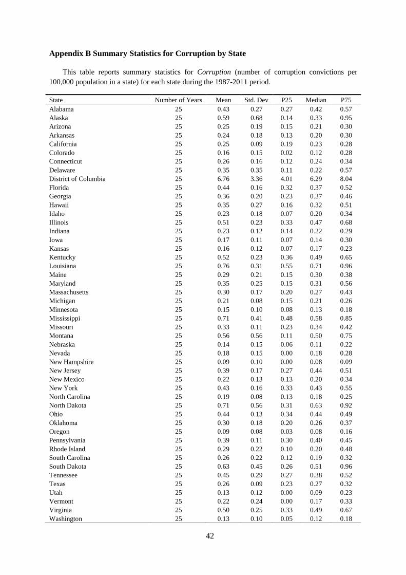
42
Appendix B Summary Statistics for Corruption by State
This table reports summary statistics for Corruption (number of corruption convictions per
100,000 population in a state) for each state during the 1987-2011 period.
State Number of Years Mean Std. Dev P25 Median P75
Alabama 25 0.43 0.27 0.27 0.42 0.57
Alaska 25 0.59 0.68 0.14 0.33 0.95
Arizona 25 0.25 0.19 0.15 0.21 0.30
Arkansas 25 0.24 0.18 0.13 0.20 0.30
California 25 0.25 0.09 0.19 0.23 0.28
Colorado 25 0.16 0.15 0.02 0.12 0.28
Connecticut 25 0.26 0.16 0.12 0.24 0.34
Delaware 25 0.35 0.35 0.11 0.22 0.57
District of Columbia 25 6.76 3.36 4.01 6.29 8.04
Florida 25 0.44 0.16 0.32 0.37 0.52
Georgia 25 0.36 0.20 0.23 0.37 0.46
Hawaii 25 0.35 0.27 0.16 0.32 0.51
Idaho 25 0.23 0.18 0.07 0.20 0.34
Illinois 25 0.51 0.23 0.33 0.47 0.68
Indiana 25 0.23 0.12 0.14 0.22 0.29
Iowa 25 0.17 0.11 0.07 0.14 0.30
Kansas 25 0.16 0.12 0.07 0.17 0.23
Kentucky 25 0.52 0.23 0.36 0.49 0.65
Louisiana 25 0.76 0.31 0.55 0.71 0.96
Maine 25 0.29 0.21 0.15 0.30 0.38
Maryland 25 0.35 0.25 0.15 0.31 0.56
Massachusetts 25 0.30 0.17 0.20 0.27 0.43
Michigan 25 0.21 0.08 0.15 0.21 0.26
Minnesota 25 0.15 0.10 0.08 0.13 0.18
Mississippi 25 0.71 0.41 0.48 0.58 0.85
Missouri 25 0.33 0.11 0.23 0.34 0.42
Montana 25 0.56 0.56 0.11 0.50 0.75
Nebraska 25 0.14 0.15 0.06 0.11 0.22
Nevada 25 0.18 0.15 0.00 0.18 0.28
New Hampshire 25 0.09 0.10 0.00 0.08 0.09
New Jersey 25 0.39 0.17 0.27 0.44 0.51
New Mexico 25 0.22 0.13 0.13 0.20 0.34
New York 25 0.43 0.16 0.33 0.43 0.55
North Carolina 25 0.19 0.08 0.13 0.18 0.25
North Dakota 25 0.71 0.56 0.31 0.63 0.92
Ohio 25 0.44 0.13 0.34 0.44 0.49
Oklahoma 25 0.30 0.18 0.20 0.26 0.37
Oregon 25 0.09 0.08 0.03 0.08 0.16
Pennsylvania 25 0.39 0.11 0.30 0.40 0.45
Rhode Island 25 0.29 0.22 0.10 0.20 0.48
South Carolina 25 0.26 0.22 0.12 0.19 0.32
South Dakota 25 0.63 0.45 0.26 0.51 0.96
Tennessee 25 0.45 0.29 0.27 0.38 0.52
Texas 25 0.26 0.09 0.23 0.27 0.32
Utah 25 0.13 0.12 0.00 0.09 0.23
Vermont 25 0.22 0.24 0.00 0.17 0.33
Virginia 25 0.50 0.25 0.33 0.49 0.67
Washington 25 0.13 0.10 0.05 0.12 0.18

43
West Virginia 25 0.36 0.22 0.22 0.28 0.49
Wisconsin 25 0.18 0.08 0.14 0.18 0.21
Wyoming 25 0.37 0.39 0.18 0.21 0.62

44
Appendix C Gravity-based Centered Index for Spatial Concentration (GCISC2)
𝐺𝐶𝐼𝑆𝐶2𝑠𝑡 = 1 − ∑ 𝑝𝑖𝑠𝑡 ×𝑖
[−1
𝐿𝑛(𝑑𝑠̅̅ ̅)
× 𝐿𝑛(𝑑𝑖𝑠) + 1]
Where 𝑝𝑖𝑠𝑡 is the number of people living in county i divided by the number of people
living in the state s in year t. 𝑑𝑖𝑠 is the distance between county i’s centroid and the state
house or assembly of state s. 𝑑𝑠̅̅ ̅ is the maximum distance between the state house or
assembly of state s’s and any point in the state.
This measure is not available in Washington DC, Hawaii, and Alaska. The geospatial
data and population data are both provided by the U.S. Census Bureau.

45
Appendix D High-Profile Political Corruption Case and Earnings Management
This table reports the OLS regression results that examine the impact of a high-profile corruption case
on discretionary accruals. In Column (1), I study how Alabama companies change their discretionary
accruals after the sentence of Don Siegelman. In Column (2), I study how Alabama companies change
their discretionary accruals after the release of Don Siegelman. The sample period is 2006 to 2007 in
Column (1), and 2007 to 2008 in Column (2). The dependent variable is DA. The indicator variable
Alabama equals 1 for Alabama firms, and 0 otherwise. The indicator variable Post_sentence equals 1
for 2007, and 0 for 2006. The indicator variable Post_release equals 1 for 2008, and 0 for 2007.
Variable definitions are provided in Appendix A. All continuous variables are winsorized at the 1st
and 99th percentiles. T statistics based on robust standard errors clustered by state-year are in
parentheses. The superscripts ***, **, and * denote statistical significance at the 1%, 5%, and 10%
levels, respectively.
(1) (2)
DA DA
Alabama * Post_sentence 0.285***
(3.007)
Post_sentence 0.010
(0.567)
Alabama * Post_release -0.461***
(-8.149)
Post_release -0.010
(-0.736)
Alabama -0.047 0.411***
(-1.422) (13.888)
Ln (total assets) -0.001 -0.003
(-0.127) (-0.456)
CFO -1.038*** -0.803***
(-10.467) (-7.148)
ROA 0.627*** 0.566***
(7.163) (6.849)
R&D -0.289*** -0.161
(-3.321) (-1.080)
R&D missing 0.017 0.036
(0.862) (1.625)
Acquisition -0.024 -0.061***
(-1.140) (-2.937)
Issuance -0.020 -0.005
(-0.916) (-0.216)
Institution -0.022 -0.072**
(-0.619) (-2.517)
Ln(Analyst) 0.013 0.003
(0.926) (0.203)
Tight covenant 0.015 0.006
(0.626) (0.235)
Meet/Beat -0.034 0.003
(-1.549) (0.124)
Sales growth -0.008 -0.041
(-0.348) (-1.301)
MB -0.003 -0.003
(-1.218) (-1.289)
Net operating assets -0.004 0.017
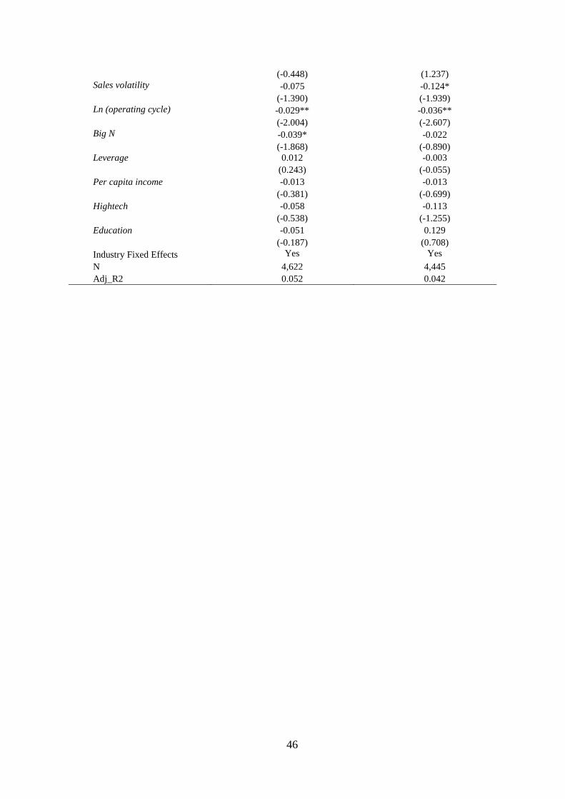
46
(-0.448) (1.237)
Sales volatility -0.075 -0.124*
(-1.390) (-1.939)
Ln (operating cycle) -0.029** -0.036**
(-2.004) (-2.607)
Big N -0.039* -0.022
(-1.868) (-0.890)
Leverage 0.012 -0.003
(0.243) (-0.055)
Per capita income -0.013 -0.013
(-0.381) (-0.699)
Hightech -0.058 -0.113
(-0.538) (-1.255)
Education -0.051 0.129
(-0.187) (0.708)
Industry Fixed Effects Yes Yes
N 4,622 4,445
Adj_R2 0.052 0.042

47
Figure 1 Map of the State Average Corruption
A map of the state average corruption data from Appendix B, where states are split into groups by the
level of political corruption.

48
Table 1 Descriptive Statistics
This table reports summary statistics during the 1987-2011 period. Panel A reports the descriptive
statistics of the full sample consisting of 56,096 observations. Panel B reports the average values of
27,836 observations in corrupt and non-corrupt groups. A firm-year observation is in the most corrupt
(least corrupt) group, if its corruption is in the top (bottom) quartile of all the observations. All sample
firms are U.S. public firms, excluding financial and utility firms. Variable definitions are provided in
Appendix A. All continuous variables are winsorized at the 1st and 99th percentiles.
Panel A Descriptive statistics for the full sample
Variable N Mean Std. Dev P25 Median P75
DA 56,096 -2.39% 30.80% -10.65% -0.92% 7.92%
Corruption 56,096 0.31 0.19 0.19 0.27 0.43
Total assets ($ million) 56,096 1796.17 5007.69 87.42 277.44 1027.02
Ln(total assets) 56,096 5.79 1.78 4.47 5.63 6.93
CFO 56,096 6.75% 18.50% 2.22% 9.07% 15.63%
ROA 56,096 0.61% 21.56% -1.16% 4.81% 9.94%
R&D 56,096 6.41% 12.12% 0.00% 0.58% 7.98%
R&D missing 56,096 0.36 0.48 0 0 1
Acquisition 56,096 0.20 0.40 0 0 0
Issuance 56,096 0.28 0.45 0 0 1
Institution 56,096 49.73% 27.49% 26.64% 49.39% 71.75%
Analyst 56,096 8.63 8.29 3 6 12
Ln(Analyst) 56,096 1.70 1.00 1.10 1.79 2.48
Tight covenant 56,096 0.11 0.32 0 0 0
Meet/Beat 56,096 0.16 0.37 0 0 0
Sales growth 56,096 24.05% 57.10% 0.77% 11.26% 28.43%
MB 56,096 3.25 3.57 1.36 2.17 3.65
Net operating assets 56,096 0.75 0.95 0.30 0.50 0.81
Sales volatility 56,096 21.90% 22.21% 8.12% 14.78% 26.96%
Operating cycle (days) 56,096 130.76 89.46 71.12 112.09 166.24
Ln(operating cycle) 56,096 4.64 0.74 4.26 4.72 5.11
Big N 56,096 0.90 0.30 1 1 1
Leverage 56,096 23.30% 24.62% 2.02% 17.88% 35.37%
Per capita Income ($10,000) 56,096 3.08 0.87 2.36 2.97 3.69
Hightech 56,096 15.31% 8.54% 8.61% 13.15% 22.08%
Education 56,096 27.14% 5.29% 23.35% 26.46% 30.45%
Panel B Descriptive statistics by non-corrupt and corrupt group
Least Corrupt Group Most Corrupt Group T-statistic difference in means
DA -1.52% -2.12% 0.594%*
Corruption 0.11 0.61 -0.500***
Ln(total assets) 5.63 5.89 -0.251***
CFO 6.61% 7.82% -1.208%***
ROA 0.16% 3.07% -2.909%***
R&D 6.75% 4.75% 2.000%***
R&D missing 0.33 0.40 -0.071***
Acquisition 0.19 0.20 -0.018***
Issuance 0.28 0.29 -0.010*
Institution 48.83% 49.23% -0.401%
Ln(Analyst) 1.69 1.67 0.013
Tight covenant 0.10 0.12 -0.019***
Meet/Beat 0.16 0.16 -0.001
Sales growth 22.43% 21.46% 0.967%

49
MB 3.12 3.19 -0.074*
Net operating assets 0.76 0.69 0.065***
Sales volatility 21.57% 21.30% 0.272%
Ln(operating cycle) 4.63 4.65 -0.019**
Big N 0.90 0.90 -0.004
Leverage 21.80% 26.12% -4.316%***
Per capita Income ($10,000) 3.06 3.01 0.047***
Hightech 16.47% 11.98% 4.488%***
Education 27.19% 27.96% -0.779%***

50
Table 2 Baseline Regression
This table reports the OLS regression results that examine the impacts of political corruption on
discretionary accrual. The sample consists of 56,096 observations. The dependent variable is DA. The
independent variable is Corruption. Column (1) reports the results where I control for all the firm-
level and state-level characteristics. Column (2) shows the results after I further control for year fixed
effects. Column (3) reports the results after I further include industry fixed effects. Variable
definitions are provided in Appendix A. All continuous variables are winsorized at the 1st and 99th
percentiles. T statistics based on robust standard errors clustered by state-year are in parentheses. The
superscripts ***, **, and * denote statistical significance at the 1%, 5%, and 10% levels, respectively.
(1) (2) (3)
DA DA DA
Corruption -0.023*** -0.021*** -0.021***
(-3.341) (-3.055) (-3.027)
Ln (total assets) -0.001 -0.001 0.001
(-0.919) (-0.973) (0.400)
CFO -0.805*** -0.810*** -0.840***
(-40.221) (-40.660) (-40.687)
ROA 0.558*** 0.564*** 0.581***
(31.597) (32.184) (32.740)
R&D -0.097*** -0.096*** -0.096***
(-4.814) (-4.736) (-4.314)
R&D missing 0.012*** 0.012*** 0.011***
(4.124) (4.020) (3.139)
Acquisition -0.011*** -0.010*** -0.011***
(-2.777) (-2.618) (-2.746)
Issuance -0.001 -0.001 -0.001
(-0.447) (-0.223) (-0.274)
Institution -0.004 -0.006 -0.003
(-0.570) (-0.844) (-0.469)
Ln(Analyst) -0.003 -0.003 -0.006***
(-1.323) (-1.319) (-2.743)
Tight covenant 0.004 0.003 0.004
(0.947) (0.584) (0.922)
Meet/Beat 0.000 0.001 0.001
(0.137) (0.243) (0.179)
Sales growth -0.006 -0.005 -0.004
(-1.429) (-1.137) (-0.896)
MB -0.001 -0.001 -0.001
(-1.417) (-1.255) (-1.421)
Net operating assets 0.004 0.003 0.001
(1.593) (1.467) (0.476)
Sales volatility -0.015* -0.017** -0.012
(-1.796) (-2.071) (-1.491)
Ln (operating cycle) -0.017*** -0.017*** -0.011***
(-7.897) (-7.856) (-3.628)
Big N -0.012** -0.012** -0.013**
(-2.542) (-2.311) (-2.557)
Leverage 0.041*** 0.041*** 0.047***
(4.539) (4.552) (5.064)
Per capita income 0.000 -0.016** -0.014**
(0.056) (-2.563) (-2.262)

51
Hightech -0.052** -0.043** -0.048**
(-2.309) (-2.027) (-2.253)
Education -0.013 0.074 0.076
(-0.289) (1.481) (1.517)
Year Fixed Effects No Yes Yes
Industry Fixed Effects No No Yes
N 56,096 56,096 56,096
Adj_R2 0.100 0.101 0.104

52
Table 3 Geographic Concentration
This table reports the subsample analysis based on firms’ geographic concentration. A firm is deemed
as concentrated (dispersed) if the percentage of operation in its headquarter state is above (below)
sample median in the year. The dependent variable is DA. The independent variable is Corruption.
Variable definitions are provided in Appendix A. All continuous variables are winsorized at the 1st
and 99th percentiles. T statistics based on robust standard errors clustered by state-year are in
parentheses. The superscripts ***, **, and * denote statistical significance at the 1%, 5%, and 10%
levels, respectively.
(1) (2)
DA DA
Concentrated Dispersed
Corruption -0.037*** -0.009
(-3.181) (-1.014)
Ln (total assets) 0.002 -0.000
(1.188) (-0.128)
CFO -0.868*** -0.822***
(-30.150) (-30.512)
ROA 0.591*** 0.595***
(22.457) (22.793)
R&D -0.039 -0.165***
(-1.368) (-3.945)
R&D missing 0.018*** 0.006
(3.209) (1.366)
Acquisition -0.011* -0.013**
(-1.741) (-2.330)
Issuance -0.001 -0.001
(-0.139) (-0.337)
Institution -0.007 -0.002
(-0.636) (-0.205)
Ln(Analyst) -0.012*** -0.002
(-3.678) (-0.658)
Tight covenant 0.014* -0.004
(1.915) (-0.703)
Meet/Beat 0.003 0.001
(0.623) (0.329)
Sales growth -0.002 -0.001
(-0.412) (-0.079)
MB -0.002** -0.000
(-2.070) (-0.193)
Net operating assets 0.003 -0.002
(0.984) (-0.518)
Sales volatility -0.005 -0.025*
(-0.396) (-1.802)
Ln (operating cycle) 0.003 -0.027***
(0.724) (-6.132)
Big N -0.023*** -0.007
(-3.030) (-0.826)
Leverage 0.035** 0.055***
(2.496) (4.616)
Per capita income -0.023** -0.009
(-2.021) (-1.166)

53
Hightech -0.075** -0.012
(-2.489) (-0.429)
Education 0.091 0.068
(1.134) (1.037)
Year Fixed Effects Yes Yes
Industry Fixed Effects Yes Yes
P value of test of equal coefficients on Corruption
between (1) and (2)
0.067*
N 25,354 25,801
Adj_R2 0.125 0.077

54
Table 4 Political Connection
This table reports the subsample analysis based on firms’ political connection. A firm is deemed as
politically connected if it registered a PAC in November of the year. The dependent variable is DA.
The independent variable is Corruption. Variable definitions are provided in Appendix A. All
continuous variables are winsorized at the 1st and 99th percentiles. T statistics based on robust
standard errors clustered by state-year are in parentheses. The superscripts ***, **, and * denote
statistical significance at the 1%, 5%, and 10% levels, respectively.
(1) (2)
DA DA
With Political Connection Without Political Connection
Corruption 0.005 -0.024***
(0.320) (-3.127)
Ln (total assets) 0.003 -0.000
(1.127) (-0.146)
CFO -0.834*** -0.840***
(-15.713) (-38.582)
ROA 0.523*** 0.587***
(9.207) (32.562)
R&D -0.076 -0.093***
(-0.895) (-4.019)
R&D missing 0.030*** 0.009**
(3.615) (2.354)
Acquisition -0.012 -0.011***
(-1.378) (-2.696)
Issuance -0.003 -0.001
(-0.430) (-0.267)
Institution -0.020 -0.001
(-1.017) (-0.156)
Ln(Analyst) 0.001 -0.006***
(0.140) (-2.859)
Tight covenant 0.003 0.004
(0.252) (0.896)
Meet/Beat -0.002 0.001
(-0.303) (0.416)
Sales growth 0.016 -0.005
(0.918) (-1.069)
MB -0.002 -0.001
(-1.369) (-1.060)
Net operating assets -0.034*** 0.004
(-3.441) (1.372)
Sales volatility -0.014 -0.014*
(-0.512) (-1.708)
Ln (operating cycle) -0.011 -0.010***
(-1.359) (-3.224)
Big N -0.014 -0.012**
(-0.681) (-2.299)
Leverage 0.048** 0.049***
(2.573) (4.972)
Per capita income -0.027 -0.013*
(-1.643) (-1.849)
Hightech -0.068 -0.044**

55
(-1.294) (-2.039)
Education 0.020 0.081
(0.155) (1.489)
Year Fixed Effects Yes Yes
Industry Fixed Effects Yes Yes
P value of test of equal coefficients on Corruption
between (1) and (2)
0.098*
N 6,812 49,284
Adj_R2 0.075 0.108

56
Table 5 Costs of Downward Earnings Management
This table reports the supsample analysis based on firms’ costs of manipulating earnings downwards.
A firm is deemed with high costs of downward earnings management, if meets or beats earnings
benchmarks at a small margin, of if it is faced with tight debt covenant, and is deemed with low costs
otherwise. The dependent variable is DA. The independent variable is Corruption. Variable
definitions are provided in Appendix A. All continuous variables are winsorized at the 1st and 99th
percentiles. T statistics based on robust standard errors clustered by state-year are in parentheses. The
superscripts ***, **, and * denote statistical significance at the 1%, 5%, and 10% levels, respectively.
(1) (2)
DA DA
High Costs Low Costs
Corruption -0.010 -0.024***
(-0.713) (-3.097)
Ln (total assets) -0.001 0.001
(-0.303) (0.673)
CFO -0.829*** -0.845***
(-23.973) (-37.772)
ROA 0.656*** 0.571***
(14.358) (30.877)
R&D -0.016 -0.104***
(-0.304) (-4.308)
R&D missing 0.025*** 0.006
(3.575) (1.552)
Acquisition -0.009 -0.012**
(-1.428) (-2.535)
Issuance -0.006 0.000
(-1.041) (0.037)
Institution -0.001 -0.003
(-0.099) (-0.300)
Ln(Analyst) -0.009** -0.005**
(-1.984) (-2.054)
Sales growth -0.011 -0.002
(-0.914) (-0.498)
MB -0.001 -0.001
(-1.519) (-1.296)
Net operating assets -0.005 0.002
(-0.916) (0.905)
Sales volatility -0.035** -0.006
(-2.117) (-0.640)
Ln (operating cycle) -0.017*** -0.009***
(-2.855) (-2.743)
Big N -0.012 -0.013**
(-1.183) (-2.285)
Leverage 0.072*** 0.041***
(5.125) (3.819)
Per capita income -0.006 -0.018**
(-0.552) (-2.412)
Hightech -0.087** -0.037
(-2.304) (-1.590)
Education -0.006 0.107**
(-0.060) (1.964)

57
Year Fixed Effects Yes Yes
Industry Fixed Effects Yes Yes
P value of test of equal coefficients on Corruption
between (1) and (2)
0.400
N 14,305 41,791
Adj_R2 0.069 0.118

58
Table 6 Alternative Measures of Corruption
This table reports the OLS regression results that examine the impacts of political corruption on
discretionary accrual by using alternative measures of corruption. In Panel A, I use the alternative
measures based on corruption convictions. In Column (1), the independent variable is Corruption per
government employee, the number of corruption convictions divided by the number of full-time
equivalent state and local government employees (in 100,000s). In Column (2), the independent
variable is Weighted corruption, per capita corruption convictions weighted by a firm’s operation in
each state. In Column (3), the independent variable is Number of convictions, the raw number of
corruption convictions divided by 1,000. In Panel B, I use the alternative measures based on
perception. In Column (1), the independent variable is Low integrity_BGA, a dummy variable that
equals 1 if the state ranks in the bottom quartile of all the states in the 2013 BGA-Alper Integrity
Index, and 0 otherwise. In Column (2), the independent variable is Low integrity_SII, a dummy
variable equals 1 if the state ranks in the bottom quartile of all the states in the 2012 State Integrity
Investigation, and 0 otherwise. In Column (3), the independent variable is Perceived corruption, the
corruption scale from Table 2 of Boylan and Long (2003). The dependent variable is DA. Variable
definitions are provided in Appendix A. All continuous variables are winsorized at the 1st and 99th
percentiles. T statistics based on robust standard errors clustered by state-year are in parentheses. The
superscripts ***, **, and * denote statistical significance at the 1%, 5%, and 10% levels, respectively.
Panel A Alternative Measures Based on Corruption Convictions
(1) (2) (3)
DA DA DA
Corruption per government employee -0.001***
(-2.848)
Weighted corruption -0.024**
(-2.020)
Number of convictions -0.116***
(-2.924)
Ln (total assets) 0.001 0.001 0.001
(0.389) (0.633) (0.486)
CFO -0.840*** -0.843*** -0.840***
(-40.683) (-37.500) (-40.672)
ROA 0.580*** 0.588*** 0.581***
(32.736) (30.942) (32.704)
R&D -0.096*** -0.090*** -0.095***
(-4.314) (-3.771) (-4.268)
R&D missing 0.011*** 0.011*** 0.011***
(3.118) (2.986) (3.202)
Acquisition -0.011*** -0.011*** -0.011***
(-2.752) (-2.785) (-2.739)
Issuance -0.001 -0.000 -0.001
(-0.280) (-0.145) (-0.294)
Institution -0.003 -0.005 -0.003
(-0.462) (-0.701) (-0.473)
Ln(Analyst) -0.006*** -0.007*** -0.006***
(-2.736) (-3.092) (-2.815)
Tight covenant 0.004 0.004 0.004
(0.927) (0.944) (0.940)
Meet/Beat 0.001 0.003 0.001
(0.182) (0.785) (0.195)

59
Sales growth -0.004 -0.002 -0.004
(-0.899) (-0.490) (-0.887)
MB -0.001 -0.001 -0.001
(-1.426) (-1.321) (-1.434)
Net operating assets 0.001 0.001 0.001
(0.479) (0.496) (0.484)
Sales volatility -0.012 -0.013 -0.012
(-1.494) (-1.385) (-1.478)
Ln (operating cycle) -0.011*** -0.011*** -0.010***
(-3.644) (-3.450) (-3.603)
Big N -0.013** -0.014*** -0.013***
(-2.542) (-2.610) (-2.617)
Leverage 0.047*** 0.044*** 0.046***
(5.064) (4.592) (5.016)
Per capita income -0.015** -0.019*** -0.011
(-2.295) (-2.752) (-1.643)
Hightech -0.044** -0.032 -0.021
(-2.088) (-1.444) (-0.958)
Education 0.075 0.097* 0.023
(1.500) (1.800) (0.440)
Year Fixed Effects Yes Yes Yes
Industry Fixed Effects Yes Yes Yes
N 56,096 51,155 56,096
Adj_R2 0.104 0.099 0.104
Panel B Alternative Measured Based on Perception
(1) (2) (3)
DA DA DA
Low integrity_BGA -0.014***
(-2.861)
Low integrity_SII -0.008*
(-1.664)
Perceived corruption -0.007**
(-2.482)
Ln (total assets) 0.000 0.000 -0.000
(0.313) (0.299) (-0.325)
CFO -0.840*** -0.840*** -0.834***
(-40.571) (-40.569) (-36.910)
ROA 0.580*** 0.580*** 0.582***
(32.668) (32.642) (31.031)
R&D -0.097*** -0.098*** -0.104***
(-4.336) (-4.383) (-4.136)
R&D missing 0.010*** 0.011*** 0.011***
(3.040) (3.072) (3.053)
Acquisition -0.011*** -0.010*** -0.010**
(-2.697) (-2.687) (-2.477)
Issuance -0.001 -0.001 -0.001
(-0.193) (-0.172) (-0.397)
Institution -0.003 -0.004 -0.009
(-0.480) (-0.519) (-1.248)
Ln(Analyst) -0.005*** -0.005*** -0.004*
(-2.634) (-2.602) (-1.775)
Tight covenant 0.004 0.004 0.005

60
(0.898) (0.889) (1.042)
Meet/Beat 0.001 0.001 0.000
(0.278) (0.250) (0.012)
Sales growth -0.004 -0.004 -0.005
(-0.864) (-0.851) (-1.134)
MB -0.001 -0.001 -0.001*
(-1.544) (-1.512) (-1.773)
Net operating assets 0.001 0.001 0.002
(0.430) (0.450) (0.656)
Sales volatility -0.012 -0.012 -0.012
(-1.444) (-1.433) (-1.374)
Ln (operating cycle) -0.011*** -0.011*** -0.011***
(-3.650) (-3.633) (-3.750)
Big N -0.013*** -0.013*** -0.012**
(-2.585) (-2.652) (-2.212)
Leverage 0.046*** 0.047*** 0.050***
(5.010) (5.039) (5.051)
Per capita income -0.018*** -0.018*** -0.014*
(-2.816) (-2.797) (-1.946)
Hightech -0.048** -0.031 -0.036
(-2.202) (-1.477) (-1.611)
Education 0.069 0.089* 0.049
(1.330) (1.705) (0.827)
Year Fixed Effects Yes Yes Yes
Industry Fixed Effects Yes Yes Yes
N 55,930 55,930 50,310
Adj_R2 0.104 0.104 0.099

61
Table 7 Restatement Likelihood
This table reports the OLS regression results that examine the impacts of political corruption on
earnings restatement. In column (1), the dependent variable is the proportion of firms understating
income in a state in a year. In column (2), the dependent variable is the proportion of firms overstating
income in a state in a year. A firm understates (overstates) net income if the original net income is
lower (higher) than restated net income. The independent variable is Corruption. The sample consists
of 1,275 state-year observations. Variable definitions are provided in Appendix A. All continuous
variables are winsorized at the 1st and 99th percentiles. T statistics based on robust standard errors
clustered by state-year are in parentheses. The superscripts ***, **, and * denote statistical
significance at the 1%, 5%, and 10% levels, respectively.
(1) (2)
% of Firms Understating Income % of Firms Overstating Income
Corruption 0.003* 0.006
(1.766) (1.292)
Per capita income -0.006* -0.002
(-1.863) (-0.198)
Hightech 0.018 0.117**
(0.956) (2.483)
Education -0.041 0.038
(-1.526) (0.531)
Year Fixed Effects Yes Yes
State Fixed Effects Yes Yes
N 1,275 1,275
Adj_R2 0.175 0.309

62
Table 8 Accounting Policy Analysis
This table examines the impacts of political corruption on alternative measures of earnings
management. I run Logit regressions in Column (1) and Column (3), and run OLS regressions in
Column (2) and Column (4). In Column (1), the dependent variables is INV method, a dummy
variable that equals 1 if the firm adopts FIFO as the primary inventory valuation method, and 0 if the
firm adopts LIFO or average cost method as the primary inventory valuation mehod. In Column (2),
the dependent variable is LIFO reserve, calculated as LIFO reserve divided by lagged total assets. In
Column (3), the dependent variable is DEP method, a dummy variable that equals 1 if the firm adopts
accelerated depreciation method, and 0 if the firm adopts straight-line depreciation method, or the mix
of accelerated depreciation method and straight-line depreciation method. In Column (4), the
dependent variable is DEP reserve, calculated as the excess amount of accumulated depreciation
divided by lagged total assets. The independent variable is Corruption. Variable definitions are
provided in Appendix A. All continuous variables are winsorized at the 1st and 99th percentiles. T
statistics based on robust standard errors clustered by state-year are in parentheses. The superscripts
***, **, and * denote statistical significance at the 1%, 5%, and 10% levels, respectively.
(1) (2) (3) (4)
INV method LIFO reserve DEP method DEP reserve
Corruption 0.100 0.009*** 0.423* 0.005*
(0.964) (4.123) (1.712) (1.937)
Ln (total assets) -0.378*** -0.000 0.362*** 0.004***
(-32.286) (-0.345) (9.202) (8.363)
CFO -0.113 -0.002 0.944** 0.007
(-0.825) (-0.225) (2.343) (1.551)
ROA 0.378*** 0.010 -0.131 -0.025***
(2.733) (0.953) (-0.364) (-5.083)
R&D 2.906*** -0.092*** 1.595*** 0.032***
(9.291) (-3.938) (3.143) (4.909)
R&D missing 0.117*** -0.003*** -0.445*** -0.010***
(3.658) (-2.700) (-4.416) (-9.362)
Acquisition 0.157*** -0.003*** -0.178 -0.016***
(4.628) (-2.648) (-1.494) (-13.615)
Issuance 0.013 -0.000 -0.126 -0.020***
(0.449) (-0.026) (-1.290) (-18.642)
Institution 0.320*** -0.001 -1.103*** 0.011***
(4.491) (-0.448) (-5.901) (5.016)
Ln(Analyst) 0.160*** -0.004*** -0.074 -0.015***
(8.558) (-5.923) (-1.040) (-22.473)
Tight covenant 0.013 -0.005*** -0.021 -0.002
(0.354) (-4.657) (-0.134) (-1.168)
Meet/Beat -0.011 0.000 -0.131 -0.002*
(-0.359) (0.051) (-1.193) (-1.664)
Sales growth 0.237*** 0.013*** -0.087 -0.027***
(5.381) (4.497) (-0.951) (-19.314)
MB -0.003 -0.001*** 0.015 0.001***
(-0.627) (-3.304) (1.037) (6.994)
Net operating assets 0.023 -0.025*** 0.181*** -0.018***
(0.838) (-15.548) (4.177) (-17.837)
Sales volatility 0.492*** -0.001 0.654*** -0.029***
(7.006) (-0.332) (3.078) (-15.625)
Ln (operating cycle) 0.193*** 0.002* -0.190** 0.004***
(6.711) (1.780) (-2.259) (4.968)
Big N -0.198*** 0.002 -0.663*** 0.003**

63
(-3.944) (0.817) (-5.046) (2.109)
Leverage 0.249*** -0.024*** -1.197*** -0.094***
(3.691) (-8.546) (-4.648) (-36.311)
Per capita income -0.100 -0.006*** -0.342* -0.000
(-1.378) (-3.254) (-1.876) (-0.131)
Hightech 2.163*** 0.001 -4.558*** 0.001
(8.160) (0.137) (-5.737) (0.176)
Education 2.388*** 0.002 4.946*** 0.030*
(3.636) (0.118) (3.412) (1.943)
Year Fixed Effects Yes Yes Yes Yes
Industry Fixed Effects Yes Yes Yes Yes
N 40,707 9,633 47,033 56,096
Adjusted_R2 0.242 0.174
Pseudo_R2 0.198 0.157

64
Table 9 Instrument Variable Approach Based on Population Concentration This table reports the second stage of a two-stage OLS regression. The dependent variable is DA. The
independent variable is Corruption. The instrument variable is the size-normalized version of Gravity-
based Centered Index for Spatial Concentration from Campante and Do (2014). The weak
instrumental variable test is a Kleibergen and Paap (2006) Wald test. Variable definitions are provided
in Appendix A. All continuous variables are winsorized at the 1st and 99th percentiles. T statistics
based on robust standard errors clustered by state-year are in parentheses. The superscripts ***, **,
and * denote statistical significance at the 1%, 5%, and 10% levels, respectively.
(1)
DA
Corruption (instrumented) -0.042**
(-2.049)
Ln (total assets) 0.001
(0.568)
CFO -0.841***
(-40.639)
ROA 0.581***
(32.750)
R&D -0.096***
(-4.283)
R&D missing 0.011***
(3.280)
Acquisition -0.011***
(-2.721)
Issuance -0.001
(-0.191)
Institution -0.003
(-0.433)
Ln(Analyst) -0.006***
(-2.747)
Tight covenant 0.004
(0.856)
Meet/Beat 0.001
(0.230)
Sales growth -0.004
(-0.850)
MB -0.001
(-1.512)
Net operating assets 0.001
(0.412)
Sales volatility -0.011
(-1.304)
Ln (operating cycle) -0.010***
(-3.557)
Big N -0.013***
(-2.661)
Leverage 0.047***
(5.028)
Per capita income -0.014**
(-2.151)
Hightech -0.062**

65
(-2.276)
Education 0.082
(1.602)
Year Fixed Effects Yes
Industry Fixed Effects Yes
Weak IV test F value 105.41
N 55,850
Adj_R2 0.105
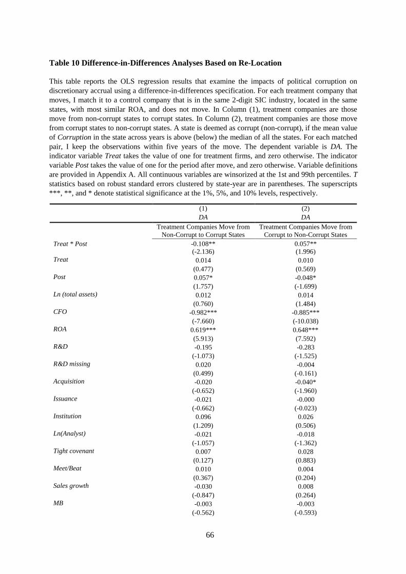
66
Table 10 Difference-in-Differences Analyses Based on Re-Location
This table reports the OLS regression results that examine the impacts of political corruption on
discretionary accrual using a difference-in-differences specification. For each treatment company that
moves, I match it to a control company that is in the same 2-digit SIC industry, located in the same
states, with most similar ROA, and does not move. In Column (1), treatment companies are those
move from non-corrupt states to corrupt states. In Column (2), treatment companies are those move
from corrupt states to non-corrupt states. A state is deemed as corrupt (non-corrupt), if the mean value
of Corruption in the state across years is above (below) the median of all the states. For each matched
pair, I keep the observations within five years of the move. The dependent variable is DA. The
indicator variable Treat takes the value of one for treatment firms, and zero otherwise. The indicator
variable Post takes the value of one for the period after move, and zero otherwise. Variable definitions
are provided in Appendix A. All continuous variables are winsorized at the 1st and 99th percentiles. T
statistics based on robust standard errors clustered by state-year are in parentheses. The superscripts
***, **, and * denote statistical significance at the 1%, 5%, and 10% levels, respectively.
(1) (2)
DA DA
Treatment Companies Move from
Non-Corrupt to Corrupt States
Treatment Companies Move from
Corrupt to Non-Corrupt States
Treat * Post -0.108** 0.057**
(-2.136) (1.996)
Treat 0.014 0.010
(0.477) (0.569)
Post 0.057* -0.048*
(1.757) (-1.699)
Ln (total assets) 0.012 0.014
(0.760) (1.484)
CFO -0.982*** -0.885***
(-7.660) (-10.038)
ROA 0.619*** 0.648***
(5.913) (7.592)
R&D -0.195 -0.283
(-1.073) (-1.525)
R&D missing 0.020 -0.004
(0.499) (-0.161)
Acquisition -0.020 -0.040*
(-0.652) (-1.960)
Issuance -0.021 -0.000
(-0.662) (-0.023)
Institution 0.096 0.026
(1.209) (0.506)
Ln(Analyst) -0.021 -0.018
(-1.057) (-1.362)
Tight covenant 0.007 0.028
(0.127) (0.883)
Meet/Beat 0.010 0.004
(0.367) (0.204)
Sales growth -0.030 0.008
(-0.847) (0.264)
MB -0.003 -0.003
(-0.562) (-0.593)

67
Net operating assets 0.025** 0.008
(2.147) (0.448)
Sales volatility -0.029 0.030
(-0.464) (0.485)
Ln (operating cycle) -0.033 -0.001
(-1.347) (-0.051)
Big N -0.082 0.057
(-1.239) (1.040)
Leverage -0.080 0.046
(-1.227) (0.803)
Per capita income 0.044 -0.024
(0.589) (-0.504)
Hightech 0.141 0.018
(0.614) (0.115)
Education 0.251 0.429
(0.471) (1.122)
Year Fixed Effects Yes Yes
Pair Fixed Effects Yes Yes
N 1,600 1,780
Adj_R2 0.072 0.136
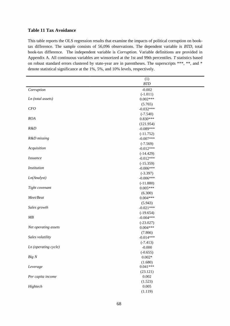
68
Table 11 Tax Avoidance
This table reports the OLS regression results that examine the impacts of political corruption on book-
tax difference. The sample consists of 56,096 observations. The dependent variable is BTD, total
book-tax difference. The independent variable is Corruption. Variable definitions are provided in
Appendix A. All continuous variables are winsorized at the 1st and 99th percentiles. T statistics based
on robust standard errors clustered by state-year are in parentheses. The superscripts ***, **, and *
denote statistical significance at the 1%, 5%, and 10% levels, respectively.
(1)
BTD
Corruption -0.002
(-1.011)
Ln (total assets) 0.002***
(5.765)
CFO -0.032***
(-7.540)
ROA 0.830***
(121.954)
R&D -0.089***
(-11.752)
R&D missing -0.007***
(-7.569)
Acquisition -0.012***
(-14.429)
Issuance -0.012***
(-15.359)
Institution -0.006***
(-3.397)
Ln(Analyst) -0.006***
(-11.880)
Tight covenant 0.005***
(6.300)
Meet/Beat 0.004***
(5.943)
Sales growth -0.021***
(-19.654)
MB -0.004***
(-23.027)
Net operating assets 0.004***
(7.866)
Sales volatility -0.014***
(-7.413)
Ln (operating cycle) -0.000
(-0.655)
Big N 0.002*
(1.680)
Leverage 0.041***
(23.121)
Per capita income 0.002
(1.523)
Hightech 0.005
(1.119)

69
Education 0.032**
(2.527)
Year Fixed Effects Yes
Industry Fixed Effects Yes
N 56,096
Adj_R2 0.891

70
Table 12 State Party Affiliation
This table reports the subsample analysis based on state party affiliation. A firm is in the Republican
(Non-Republican) subsample, if the governor of the firm’s headquarter state is an Republican (not an
Republican). The dependent variable is DA. The independent variable is Corruption. Variable
definitions are provided in Appendix A. All continuous variables are winsorized at the 1st and 99th
percentiles. T statistics based on robust standard errors clustered by state-year are in parentheses. The
superscripts ***, **, and * denote statistical significance at the 1%, 5%, and 10% levels, respectively.
(1) (2)
DA DA
Republican Non-Republican
Corruption -0.023** -0.031***
(-2.503) (-2.898)
Ln (total assets) 0.000 0.001
(0.022) (0.673)
CFO -0.837*** -0.844***
(-33.902) (-23.340)
ROA 0.561*** 0.611***
(24.067) (24.043)
R&D -0.136*** -0.025
(-4.760) (-0.747)
R&D missing 0.010** 0.012**
(2.158) (2.257)
Acquisition -0.010** -0.009
(-2.241) (-1.373)
Issuance 0.001 -0.002
(0.304) (-0.407)
Institution 0.011 -0.024**
(1.213) (-2.081)
Ln(Analyst) -0.005* -0.007**
(-1.698) (-2.317)
Tight covenant 0.001 0.009
(0.184) (1.156)
Meet/Beat 0.005 -0.005
(1.189) (-1.066)
Sales growth 0.002 -0.011
(0.321) (-1.382)
MB -0.001 -0.001
(-0.940) (-1.390)
Net operating assets 0.000 0.002
(0.147) (0.472)
Sales volatility -0.005 -0.024**
(-0.434) (-2.019)
Ln (operating cycle) -0.009** -0.013***
(-2.496) (-2.740)
Big N -0.015** -0.013
(-2.422) (-1.485)
Leverage 0.041*** 0.053***
(3.690) (3.350)
Per capita income 0.003 -0.032***
(0.322) (-3.527)
Hightech -0.044* -0.035

71
(-1.706) (-0.999)
Education -0.041 0.191***
(-0.607) (2.840)
Year Fixed Effects Yes Yes
Industry Fixed Effects Yes Yes
P value of test of equal coefficients on Corruption
between (1) and (2)
0.581
N 33,409 22,521
Adj_R2 0.113 0.0952