Political Risk Reinsurance Pricing – A Capital Market Approach Athula Alwis, Vladimir Kremerman, Yakov Lantsman, Jason Harger and Junning Shi

Willis Analytics Willis Re Inc. Abstract: Political risk insurance is concerned with the risk associated with government intervention and restriction of trade into emerging markets. It may encompass long-term perils (investment related), such as the confiscation, expropriation or nationalization of an infrastructure project in an emerging market or short term perils (export trade related), such as contract frustration, embargo or currency inconvertibility. Today exposure to the political will of a host country is being challenged by economic events blurring the landscape for political risk, which is creating a growing need for better informed econometrics, and advanced analysis of risk vs. reward, as well as a broader interpretation of covered perils and events. The need for reinsurance capacity in Political Risk is higher than it has been in a decade. However, more and more reinsurers are either restricting the coverage or entirely leaving the practice. This paper proposes an objective reinsurance pricing methodology to assess the risk of writing a large political risk reinsurance portfolio based on country risk ratings, sovereign ceilings, political risk default rates and severity assumptions based on historical data. The paper also incorporates a mechanism to indicate the effects of regional and trade correlations based on the advanced credit modeling. Having such an objective methodology to assess the risk of reinsuring political risk should broaden support from traditional reinsurance markets and attract risk capital from the capital markets. Key Words: Confiscation, Contract Frustration, Contract Repudiation, Correlation, Country Risk Ratings, Currency Inconvertibility, Default Rates, Exchange Transfer, Expropriation, Gaussian Copula, Nationalization, Recovery Rates, Merton Model, Reinsurance, Sovereign Ceiling, Wrongful Calling of Guarantee

- 1 -

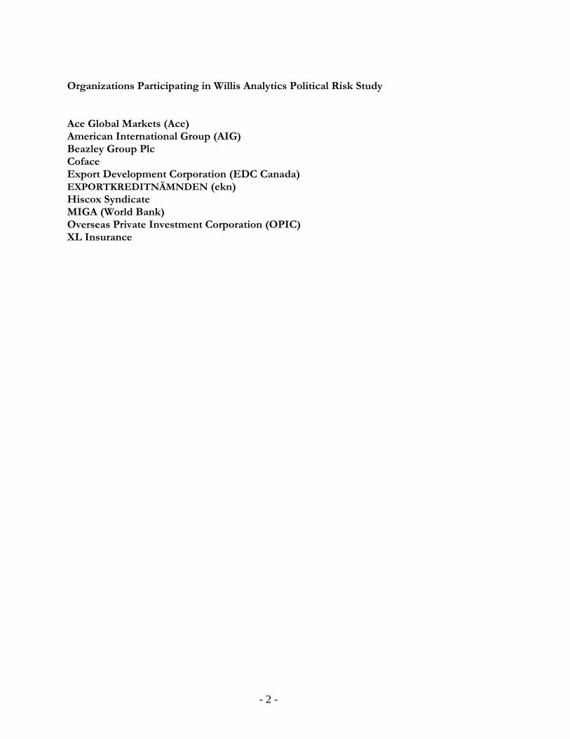
Organizations Participating in Willis Analytics Political Risk Study Ace Global Markets (Ace) American International Group (AIG) Beazley Group Plc Coface Export Development Corporation (EDC Canada) EXPORTKREDITNÄMNDEN (ekn) Hiscox Syndicate MIGA (World Bank) Overseas Private Investment Corporation (OPIC) XL Insurance

- 2 -

Section 1: Introduction The underwriting evaluation of a political risk portfolio to provide reinsurance capacity is one of the toughest and most complex decisions made by reinsurers today. There is enormous uncertainty in assessing the risk-return profile of any reinsurance cover. The sheer complexity of the underlying business makes it nearly impossible to quantify profitability in political risk reinsurance using existing actuarial risk evaluation methodologies such as trending and developing past losses to estimate future claims. The Argentinean crisis in 2001 forced several reinsurers to either reduce the reinsurance capacity they provided or leave the political risk reinsurance arena altogether. The crisis was a serious wake up call to many reinsurers regarding the need for consistent and objective risk evaluation and management processes - even if they were not appropriately awakened by the 1997 Asian financial crisis and the 1999 Russian debt crisis. The Argentinean crisis alerted reinsurers to the massive political risk exposures in developing and emerging markets. The media assertions of large losses without understanding the probabilities of default and the relatively small percentage of loss given default added greater pressure on senior management to make tough business decisions. The reinsurers who decided to remain in the political risk business were required to justify to senior management not only that the business is profitable in the long run but also there are objective criteria to quantify the risk. The primary goal of this paper is to propose an objective methodology to quantify the risk-return profile of a political risk insurer for the purpose of providing reinsurance capacity. This methodology will also allow political risk insurance and reinsurance carriers to evaluate their own portfolios for overall profitability and capital requirements to support the on-going business. Political Risk can be defined as the company’s exposure to the risk of a political event that would diminish the value of an investment or a loan. The major political risk covers (classes) are:

1. Currency Inconvertibility (CI) and Exchange Transfer (FX) 2. Confiscation, Expropriation and Nationalization (CEN) 3. Political Violence (PV) or War (including revolution, insurrection, politically motivated civil strife,

terrorism) 4. Breach of Contract, Contract Frustration (CF), Contract Repudiation (CR) 5. Wrongful Calling of Guarantee (WCG)

1. Currency Inconvertibility (CI) and Exchange Transfer (FX):

• Inability of an investor/lender to convert profits, investment returns and debt service from local currency to hard currency ($ € £)

• Inability of an investor/lender to transfer hard currency out of the country of risk 2. Confiscation, Expropriation and Nationalization (CEN):

• Loss of funds or assets due to confiscation, expropriation, or nationalization by the host government of the country of risk

- 3 -

• Any unlawful action by the host government depriving the investor of fundamental rights in a project (creeping expropriation)

3. Political Violence (PV) or War (including revolution, insurrection, politically motivated civil strife, terrorism)

• Loss of funds or assets due to political violence or war 4. Breach of Contract, Contract Frustration (CF), Contract Repudiation (CR)

• Loss of funds or assets due to arbitrary non-honoring of a contract by a foreign government (or a semi government entity) or breach of contract by a private business entity due to an arbitrary act of a foreign government

• Loss of funds due to non-payment of a loan or guarantee 5. Wrongful Calling of Guarantee (WCG)

• Loss of funds or assets due to the host government arbitrarily calling its bonds or a business entity being forced to call guarantees due to political events (the bonds are generally backed by irrevocable letters of credit which are callable on demand)

Section 2: Data Willis Analytics has created a comprehensive database combining the data contributed by the industry participants. The database contains over 15,000 records covering 180 countries. The loss data covers years 1966 through 2004 while the corresponding policy limits are not always available. The data is available by year, country, and risk type (form). The loss data is also available in its component parts (paid loss, loss reserve, recoveries) on a limited basis. The policy information (policy counts and aggregate limits by country and year) is available for the most part on an aggregate basis. Section 3: Proposed Methodology The proposed methodology will create a consistent and objective framework to conduct a portfolio level analysis of a political risk book of business. It is based on developing a distribution of political risk losses that would support the determination of Value at Risk (VAR) and/or Tail Value at Risk (TVAR) to determine the capital requirements to conduct the business that is being analyzed. In addition, the methodology facilitates analysis of underwriting profitability, return on capital, reinsurance pricing, and many other underwriting and financial measurements. The development of loss distributions at portfolio and policy level is based on the entity’s political risk exposure by country, long term country risk ratings, percentage of defaults within a country, political risk default rates, severity rates, and regional/trade correlation assumptions. This level of granularity provides the ability to establish the portfolio and marginal rate of returns in order to objectively determine the price for political risk.

- 4 -

The conceptual framework

• Application of Generalized Linear Models (GLM) to derive expected default rates by form/class based on historical default rates and statistically significant country specific macro economic factors such as gross domestic product, inflation, unemployment rates, political stability indexes et cetera.

• Analysis of country specific macro economic factors to derive the political risk default dependence between countries to develop input assumptions for the correlation matrix

• Usage of the Generalized Linear Models (GLM) framework to derive recovery rates by form/class • Combination of derived default rates by form and event correlation assumptions by country/region

to achieve reasonable pair-wise correlation factors • Aggregation of loss distributions by simulating correlated default events and corresponding

simulated losses by country and form The Process The aggregate loss distribution at policy and portfolio level will be produced by simultaneously simulated processes:

• Simulation of the correlated econometric and political scenarios • Recovery rates simulations • Loss aggregation across portfolio

Loss Distribution = ƒ(A, D, C, N, L) A = Projected Country Aggregate Exposure by class of risk D = Political Risk Default Rate by class of risk C = Correlation Matrix N = Percentage of Defaults within a Sovereign Nation (given that the country is in default) L = Percentage of Loss Net of Recoveries (given that the limit is in default)

• The country aggregate exposure by class of risk per a given country represents the sum of all limits within a sovereign nation for a given class of risk (CEN, CI, etc.)

• The political risk default rate by class of risk represents default rates calculated based on historical

data or prospective default rates based on non-linear regression.

• The correlation matrix contains the dependence structure between countries in the political risk portfolio being analyzed.

• The percentage of defaults within a sovereign nation represents sum of limits in default compared to

the total aggregate exposure in the entire country

• The percentage of loss net of recoveries is estimated by the ultimate loss compared to the total limit that is in default

- 5 -

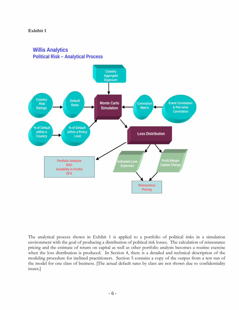
Exhibit 1

Country Risk

Ratings Monte CarloSimulation

CountryAggregateExposure

Profit MarginCapital Charge

CorrelationMatrix

Willis AnalyticsPolitical Risk – Analytical Process

Loss Distribution

Indicated LossExpenses

ReinsurancePricing

Portfolio AnalysisROC

Variability in ProfitsDFA

% of Defaultwithin a Country

% of Defaultwithin a Policy

Limit

DefaultRates Event Correlation

& Pair-wiseCorrelation

The analytical process shown in Exhibit 1 is applied to a portfolio of political risks in a simulation environment with the goal of producing a distribution of political risk losses. The calculation of reinsurance pricing and the estimate of return on capital as well as other portfolio analysis becomes a routine exercise when the loss distribution is produced. In Section 4, there is a detailed and technical description of the modeling procedure for inclined practitioners. Section 5 contains a copy of the output from a test run of the model for one class of business. [The actual default rates by class are not shown due to confidentiality issues.]

- 6 -

Section 4: Modeling a Political Risk Portfolio The modeling of a political risk portfolio consists of several key steps:

1. Development of default rates 2. Development of percentage of loss within a policy limit (i.e. 1 – recovery rate) 3. Development of percentage of defaults within a sovereign nation given that the country is in

default 4. Development of a correlation matrix

1. The development of expected default rates The development of default rates consist of four parts:

a) default rates based on historical data The authors define “default rate” as number of claims divided by number of policies. The “country year” is defined as one sovereign nation with any type of political risk coverage for one full year. Moreover, the “defaulted country year” is defined as a country year with at least one political risk default within the country of risk. There are two sets of default rates calculated in this study.

• default rates by class (CI/FX, CEN, PV/War, CF/CR, WCG) • default rate per country year

In addition, the ratio of number of defaulted country years divided by total country years is compared to the ratio of total claims divided by total policy counts. The historical data is provided by the participating entities listed at the beginning of this paper.

b) Prospective default rates based on macro economic variables and political indicators Prospective political risk events can be modeled based on the binary situation of occurrence or non-occurrence of a political risk event. Limited Dependent Variable (LDV) theory presents a methodology to map continuous characteristics into a discrete set of variables via nonlinear regression. The most used examples of this methodology are logit and probit models. Academic researchers suggest that the country-specific political risks are highly correlated with a country’s macroeconomic variables and political stability indicators. Among the suggested list of explanatory variables are GDP per capita, inflation, current account deficit, exchange rate, political stability indicators, and government effectiveness indicators. For the purpose of calibrating the predictive model, the historical default rates of political risk events are calculated from the data base provided by participating entities. The statistical data of the macroeconomic variables and the

- 7 -

political indicators come from the International Monetary Fund (World Economic Outlook database) as well as the World Bank (World Development Indicators database). Logistic regression analysis describes how a binary response variable is associated with a set of explanatory variables. It is a member of the family of Generalized Linear Models (GLM) in which the mean of a response variable is related to explanatory variables through a regression equation: pp XXg βββμ +++= ...)( 110 , where g(µ) is the link function that is chosen according to the distribution of the response variable. In general, the natural link for a binary response variable is the logit function. The predictive model that is fitted to forecast probabilities of the future occurrences of political risk events is shown below:

pp XXd

d βββ +++=−

...)1

log( 110 ,

where d is the political risk default rate and X1 through Xp are economic variables and political indicators that explain the occurrence of the political risk events. An alternative to logistic regression for binary responses is to choose g(d) to be the inverse of the cumulative standard normal probability distribution function, i.e., g(d) equals the 100dth percentile in the standard normal distribution. The default rate d is assumed to follow a logistic distribution under the logistic regression or a normal distribution under the probit regression. MIGA (World Bank) has used statistical analysis and non-linear regression to project default rates based on past MIGA experience and judgment (Hamada, J. 2004) similar to the process outlined above.

c) Distribution of average default rates by rating category Discriminant Function Analysis is used to determine the linear combinations of variables that best discriminate the subjects in different categories. For example, Discriminant Function Analysis can be used to investigate which variables discriminate between countries that fall into the country rating categories from Aaa to D similar to Moody’s sovereign ceilings.

In the two-group case, the Discriminant Function Analysis can also be thought of as a multiple regression. The grouping category is used as the dependent variable and the economic variables are used as independent variables in a multiple regression analysis, then the results are analogous to those obtained via Discriminant Function Analysis. In general, the two group discriminant function is illustrated as:

pp XbXbXbaGroup ++++= ...2211 ,

where Group is the country rating category and X1 through Xp are macroeconomic variables and political indicators.

The number of discriminant functions that is needed to solve the generalized version is one less than the number of groups. The relevant output from discriminant analysis consists of the coefficients of the discriminant functions, the discriminant function scores for each subject, measures of the percentage of cases correctly classified by the analysis, and an overall measure of group differences. The discriminant

- 8 -

functions and scores that are estimated from historical data can be applied to classify future country-year combination into different rating categories based on the projection of macroeconomic and political indicators of a country.

d) Distribution of average default rates based on duration

Curves are fitted to political risk default rates by class based on the time of default (short term, medium term, and long term). The fitted curves are used to distribute the average default rates by class into a table of default rates that vary by duration. The outcome of this process is a table of expected default rates by rating class and duration. In addition, this methodology presents an opportunity to simulate future default rates based on country specific (or region specific) macro economic factors and correlations derived from the same factors. 2. The development of percentage of loss within a policy limit (i.e. severity rate) The severity rate can be defined as the ratio of ultimate loss divided by the policy limit. There are two sets of severity rates calculated in this study that are based on data provided by participating entities.

1. severity rates by class (CI/FX, CEN, PV/War, CF/CR, WCG) 2. severity rate per country year

3. The development of percentage of defaults within a sovereign nation given that the country is

in default The percentage of defaults within a country can be defined as total policy limits in default within the country divided by the total aggregate policy limits. The available data to estimate this ratio is sparse. Therefore, a confidence interval is established and the ratio is allowed to fluctuate within this range during the simulation process. 4. The development of a correlation matrix A key feature of the proposed methodology is the inclusion of correlated events, either regional, or trade, in the estimation of losses. The global economy is inter-related as never before. In addition to obvious political and economic influences between countries that are geographically connected, there are strong and long-standing trade relationships between these countries. An economic downturn or a political upheaval in one country could adversely affect another country that is connected via proximity or trade. It is the authors’ attempt to model the potential adverse effect of correlated political risk events to the portfolio under consideration by utilizing a correlation matrix in Monte Carlo simulation. The easier method is to consider a fixed time horizon model and use a Gaussian copula to incorporate the correlation matrix. The harder and perhaps more appropriate method is to use a multi-year model with a Gaussian copula or an

- 9 -

Archimedean copula where the time of loss is taken into account in simulation (in addition to whether there is a loss event or not). The key idea is to model several large political risk losses within the portfolio while capturing the timing risk of defaults to assess the capital need to withstand an extreme event. The input for the correlation matrix would come from two sources.

• The dependence quantified in the Generalized Linear Modeling of macro economic factors • Judgment based on empirical data

Technical details on correlation and copulas are provided in Appendix A.

- 10 -

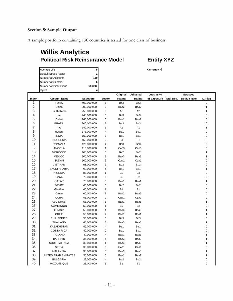
Section 5: Sample Output A sample portfolio containing 130 countries is tested for one class of business:

Willis AnalyticsPolitical Risk Reinsurance Model Entity XYZAverage Life 5 Currency: €Default Stress Factor 1Number of Accounts 130Number of Sectors 6Number of Simulations 50,000 layers 4

Original Adjusted Loss as % StressedIndex Account Name Exposure Sector Rating Rating of Exposure Std. Dev. Default Rate IG Flag

1 Turkey 400,000,000 6 Ba3 Ba3 02 China 300,000,000 3 Baa2 Baa2 13 South Korea 250,000,000 3 A2 A2 14 Iran 240,000,000 5 Ba3 Ba3 05 Dubai 240,000,000 5 Baa1 Baa1 06 BRAZIL 200,000,000 2 Ba3 Ba3 07 Iraq 180,000,000 5 A1 A1 18 Russia 175,000,000 4 Ba1 Ba1 09 INDIA 150,000,000 3 Ba1 Ba1 010 INDONESIA 150,000,000 3 B1 B1 011 ROMANIA 125,000,000 4 Ba3 Ba3 012 ANGOLA 110,000,000 1 Caa3 Caa3 013 MOROCCO 105,000,000 5 Ba2 Ba2 114 MEXICO 100,000,000 2 Baa3 Baa3 115 SUDAN 100,000,000 5 Caa1 Caa1 016 VIET NAM 95,000,000 3 Ba3 Ba3 017 SAUDI ARABIA 90,000,000 5 Ba1 Ba1 118 NIGERIA 85,000,000 1 B3 B3 019 Libiya 75,000,000 5 B2 B2 020 QATAR 75,000,000 5 Baa1 Baa1 121 EGYPT 65,000,000 5 Ba2 Ba2 022 GHANA 60,000,000 1 B1 B1 023 Oman 60,000,000 5 Baa2 Baa2 024 CUBA 55,000,000 2 Caa1 Caa1 025 ABU-DHABI 55,000,000 5 Baa1 Baa1 126 CAMEROON 50,000,000 1 B2 B2 027 TUNISIA 50,000,000 1 Baa3 Baa3 128 CHILE 50,000,000 2 Baa1 Baa1 129 PHILIPPINES 50,000,000 3 Ba3 Ba3 030 THAILAND 45,000,000 3 Baa3 Baa3 131 KAZAKHSTAN 45,000,000 4 Ba1 Ba1 032 COSTA RICA 40,000,000 2 Ba1 Ba1 033 POLAND 40,000,000 4 Baa1 Baa1 134 BAHRAIN 35,000,000 5 Baa3 Baa3 135 SOUTH AFRICA 35,000,000 1 Baa3 Baa3 136 SYRIA 30,000,000 5 Caa1 Caa1 037 MALAYSIA 30,000,000 3 Baa3 Baa3 138 UNITED ARAB EMIRATES 30,000,000 5 Baa1 Baa1 139 BULGARIA 25,000,000 4 Ba2 Ba2 040 MOZAMBIQUE 25,000,000 1 B1 B1 0

- 11 -

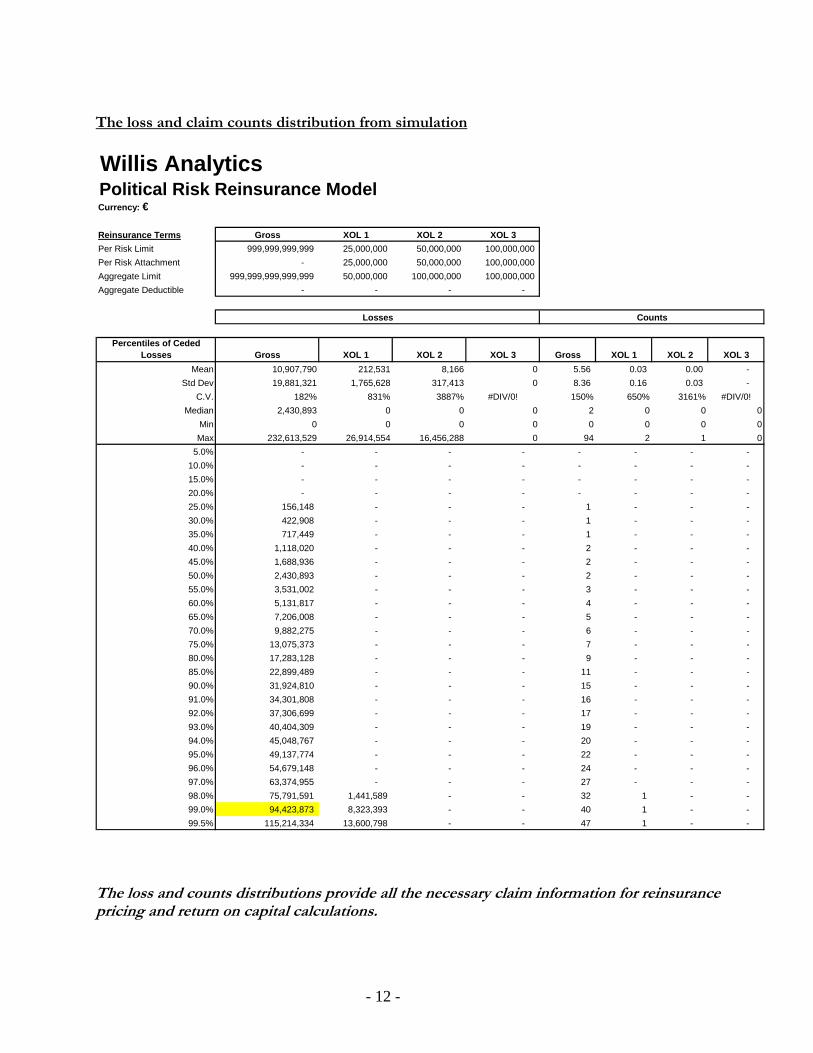
The loss and claim counts distribution from simulation

Willis AnalyticsPolitical Risk Reinsurance ModelCurrency: €

Reinsurance Terms Gross XOL 1 XOL 2 XOL 3Per Risk Limit 999,999,999,999 25,000,000 50,000,000 100,000,000 Per Risk Attachment - 25,000,000 50,000,000 100,000,000 Aggregate Limit 999,999,999,999,999 50,000,000 100,000,000 100,000,000 Aggregate Deductible - - - -

Percentiles of Ceded Losses Gross XOL 1 XOL 2 XOL 3 Gross XOL 1 XOL 2 XOL 3

Mean 10,907,790 212,531 8,166 0 5.56 0.03 0.00 - Std Dev 19,881,321 1,765,628 317,413 0 8.36 0.16 0.03 -

C.V. 182% 831% 3887% #DIV/0! 150% 650% 3161% #DIV/0!Median 2,430,893 0 0 0 2 0 0 0

Min 0 0 0 0 0 0 0 0Max 232,613,529 26,914,554 16,456,288 0 94 2 1 0

5.0% - - - - - - - - 10.0% - - - - - - - - 15.0% - - - - - - - - 20.0% - - - - - - - - 25.0% 156,148 - - - 1 - - - 30.0% 422,908 - - - 1 - - - 35.0% 717,449 - - - 1 - - - 40.0% 1,118,020 - - - 2 - - - 45.0% 1,688,936 - - - 2 - - - 50.0% 2,430,893 - - - 2 - - - 55.0% 3,531,002 - - - 3 - - - 60.0% 5,131,817 - - - 4 - - - 65.0% 7,206,008 - - - 5 - - - 70.0% 9,882,275 - - - 6 - - - 75.0% 13,075,373 - - - 7 - - - 80.0% 17,283,128 - - - 9 - - - 85.0% 22,899,489 - - - 11 - - - 90.0% 31,924,810 - - - 15 - - - 91.0% 34,301,808 - - - 16 - - - 92.0% 37,306,699 - - - 17 - - - 93.0% 40,404,309 - - - 19 - - - 94.0% 45,048,767 - - - 20 - - - 95.0% 49,137,774 - - - 22 - - - 96.0% 54,679,148 - - - 24 - - - 97.0% 63,374,955 - - - 27 - - - 98.0% 75,791,591 1,441,589 - - 32 1 - - 99.0% 94,423,873 8,323,393 - - 40 1 - - 99.5% 115,214,334 13,600,798 - - 47 1 - -

Losses Counts

The loss and counts distributions provide all the necessary claim information for reinsurance pricing and return on capital calculations.

- 12 -

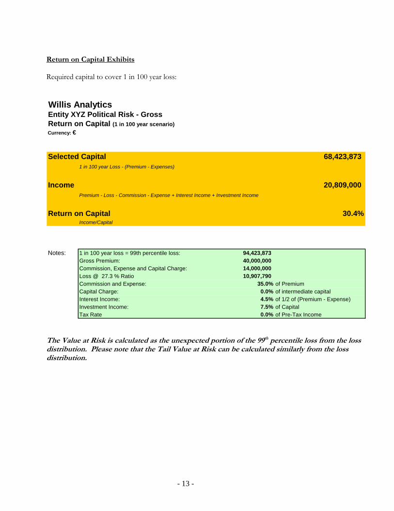
Return on Capital Exhibits Required capital to cover 1 in 100 year loss: Willis AnalyticsEntity XYZ Political Risk - GrossReturn on Capital (1 in 100 year scenario)Currency: €

Selected Capital 68,423,873 1 in 100 year Loss - (Premium - Expenses)

Income 20,809,000 Premium - Loss - Commission - Expense + Interest Income + Investment Income

Return on Capital 30.4%Income/Capital

Notes: 1 in 100 year loss = 99th percentile loss: 94,423,873 Gross Premium: 40,000,000 Commission, Expense and Capital Charge: 14,000,000 Loss @ 27.3 % Ratio 10,907,790 Commission and Expense: 35.0% of PremiumCapital Charge: 0.0% of intermediate capitalInterest Income: 4.5% of 1/2 of (Premium - Expense)Investment Income: 7.5% of CapitalTax Rate 0.0% of Pre-Tax Income

The Value at Risk is calculated as the unexpected portion of the 99th percentile loss from the loss distribution. Please note that the Tail Value at Risk can be calculated similarly from the loss distribution.

- 13 -

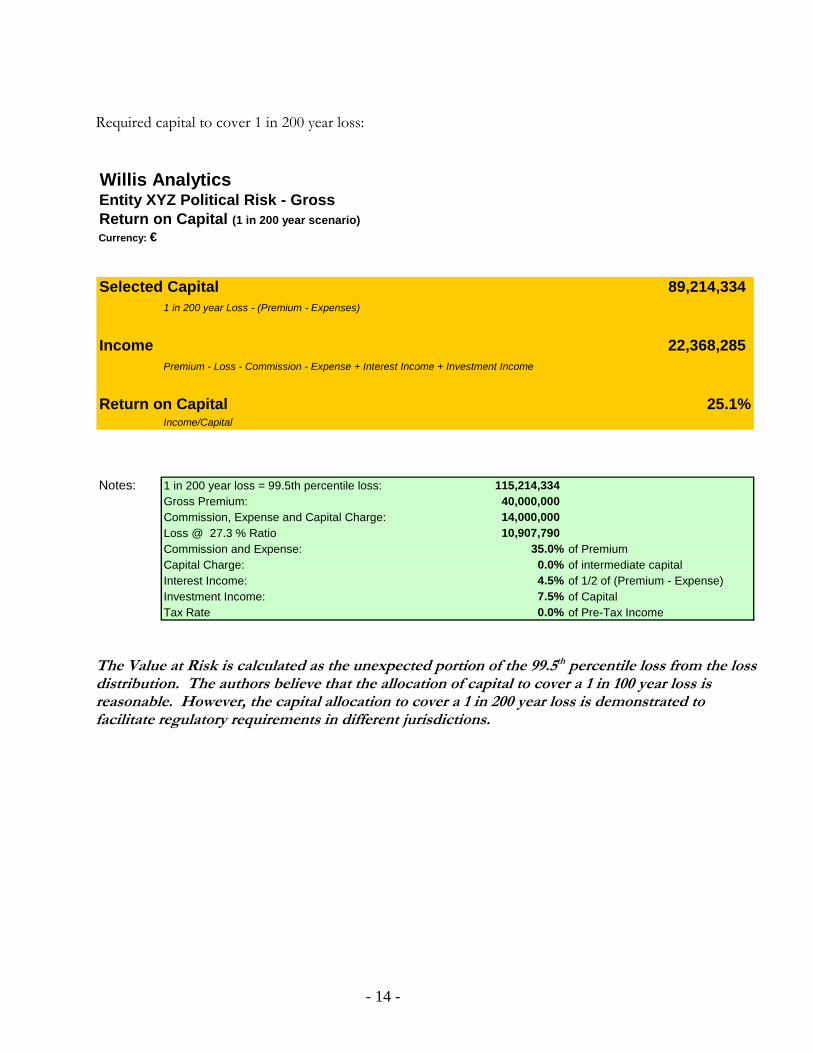
Required capital to cover 1 in 200 year loss: Willis AnalyticsEntity XYZ Political Risk - GrossReturn on Capital (1 in 200 year scenario)Currency: €

Selected Capital 89,214,334 1 in 200 year Loss - (Premium - Expenses)

Income 22,368,285 Premium - Loss - Commission - Expense + Interest Income + Investment Income

Return on Capital 25.1%Income/Capital

Notes: 1 in 200 year loss = 99.5th percentile loss: 115,214,334 Gross Premium: 40,000,000 Commission, Expense and Capital Charge: 14,000,000 Loss @ 27.3 % Ratio 10,907,790 Commission and Expense: 35.0% of PremiumCapital Charge: 0.0% of intermediate capitalInterest Income: 4.5% of 1/2 of (Premium - Expense)Investment Income: 7.5% of CapitalTax Rate 0.0% of Pre-Tax Income

The Value at Risk is calculated as the unexpected portion of the 99.5th percentile loss from the loss distribution. The authors believe that the allocation of capital to cover a 1 in 100 year loss is reasonable. However, the capital allocation to cover a 1 in 200 year loss is demonstrated to facilitate regulatory requirements in different jurisdictions.

- 14 -

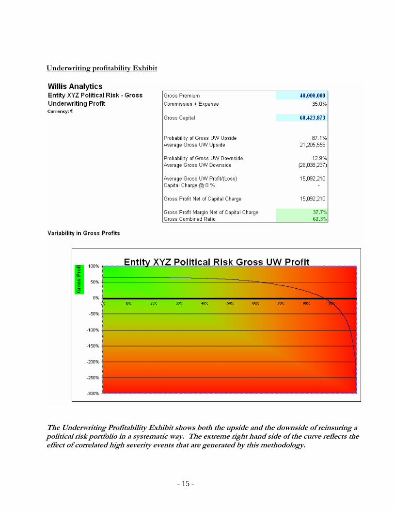
Underwriting profitability Exhibit

The Underwriting Profitability Exhibit shows both the upside and the downside of reinsuring a political risk portfolio in a systematic way. The extreme right hand side of the curve reflects the effect of correlated high severity events that are generated by this methodology.

- 15 -

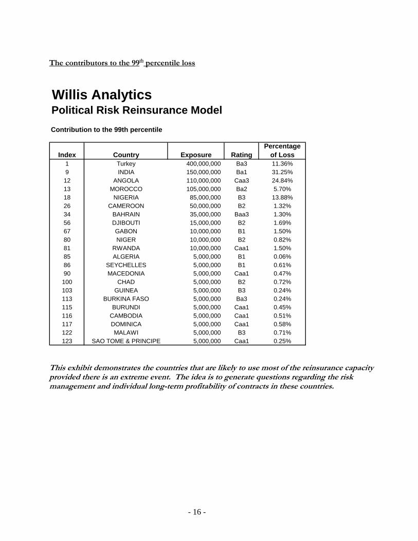
The contributors to the 99th percentile loss

Willis AnalyticsPolitical Risk Reinsurance ModelContribution to the 99th percentile

Index Country Exposure RatingPercentage

of Loss1 Turkey 400,000,000 Ba3 11.36%9 INDIA 150,000,000 Ba1 31.25%

12 ANGOLA 110,000,000 Caa3 24.84%13 MOROCCO 105,000,000 Ba2 5.70%18 NIGERIA 85,000,000 B3 13.88%26 CAMEROON 50,000,000 B2 1.32%34 BAHRAIN 35,000,000 Baa3 1.30%56 DJIBOUTI 15,000,000 B2 1.69%67 GABON 10,000,000 B1 1.50%80 NIGER 10,000,000 B2 0.82%81 RWANDA 10,000,000 Caa1 1.50%85 ALGERIA 5,000,000 B1 0.06%86 SEYCHELLES 5,000,000 B1 0.61%90 MACEDONIA 5,000,000 Caa1 0.47%

100 CHAD 5,000,000 B2 0.72%103 GUINEA 5,000,000 B3 0.24%113 BURKINA FASO 5,000,000 Ba3 0.24%115 BURUNDI 5,000,000 Caa1 0.45%116 CAMBODIA 5,000,000 Caa1 0.51%117 DOMINICA 5,000,000 Caa1 0.58%122 MALAWI 5,000,000 B3 0.71%123 SAO TOME & PRINCIPE 5,000,000 Caa1 0.25%

This exhibit demonstrates the countries that are likely to use most of the reinsurance capacity provided there is an extreme event. The idea is to generate questions regarding the risk management and individual long-term profitability of contracts in these countries.

- 16 -

Section 6: Conclusion It is our belief that the proposed methodology will provide actuaries and financial analysts with the ability to consistently and objectively quantify the risk of writing a political risk portfolio. It will facilitate the estimation of Value at Risk, Tail Value at Risk, Required Capital, Return on Capital, and Underwriting Profitability for a given political risk portfolio by reinsurers and capital markets. Given that the analytical processes and country rating systems of the primary political risk carriers are already in place, the data and analytical tools are available to apply this methodology to evaluate the risk-return profile of a political risk portfolio. The authors strongly believe that applying this approach would give organizations involved in political risk insurance and reinsurance a solid foundation for making strategic and business decisions.

- 17 -

Appendix A The fixed-time horizon model

Correlation is the degree to which two or more quantities are linearly associated. In a two-dimensional plot, the degree of correlation between the values on the two axes is quantified by the so-called correlation coefficient.

According to Li (1999): the linear correlation of default for two securities i and j, ijρ satisfies the following equation

)1()1()1(

),()()(

),(

jjiiij uuuu

jiCovjVariVar

jiCov−−

=⋅

=ρ ,

where are corresponding default probabilities. The approach the authors used to incorporate correlation into the simulation engine is described below. Any attempt to simulate credit events without giving appropriate regard to the effects of correlation would severely underestimate the tail of the distribution.

ji uu ,

It is necessary to compute using the within and between correlations assumptions determined at the outset of the analysis. The authors use Merton’s approach to calculate . The Merton approach to the firm’s value suggests that a default occurs when the value of assets is below certain threshold (Merton (1974)). In other words, default takes place when a random variable representing firm’s assets X

),( jiCov),( jiCov

i (with CDF ) is below a certain level. Two companies are in default if . Then the

covariance equals to )( iXP )(),( 11

jjii uPXuPX −− <<

jiji uuuPuPP −−− ))(),(( 11 In order to generate credit events (defaults), Monte Carlo simulation is applied. A set of independent normal random variables are transformed to a correlated standard normal random variables by introducing a correlation matrix to the process. The correlated standard normal random variables are compared to the thresholds based on default rates. The correlation matrix needs to be decomposed based on the Cholesky decomposition prior to creating a matrix of correlated standard random variables. There are two key adjustments that are necessary to obtain a reasonable set of outcomes. They are outlined below. The Merton Adjustment The most straightforward approach in the calculation of a copula in the above equation is to assume that Xi , Xj are normally distributed. Then, one obtains for coefficient of correlation (Pugachevsky (2002))

)2()1()1(

)),(),(( 11)2(

jjii

jiMijji

ij uuuu

uuuNuNN

−−

−=

−− ρρ .

In equation (2), is the cumulative bivariate normal distribution function with pair-wise correlation coefficient and is the inverse of standard normal distribution. The matrix is determined numerically from Eq.(2) and is used in the loss simulation. After pair-wise correlation coefficients are computed, the simulation engine can produce a correlated multi-variate distribution. According to Pugachevsky (2002), the main advantage of this method is that it is easy to define correlations between random variables in a simulation environment.

)2(NMijρ )1(−N M

ijρ

- 18 -

The resulting correlation is materially higher than the discrete events correlationMijρ ijρ . It should be noted

that the use of events correlation ijρ in simulation would lead to substantial underestimation of the correlation effect. How to make the correlation matrix positive-definite The resulting correlation matrix obtained from Eq. (2) is not necessarily positive-definite. The positive-definiteness is a requirement that guarantees the ability to decompose the correlation matrix after the application of Merton adjustment. There are several known techniques that would help transform the correlation matrix into a positive definite matrix. The authors chose the approach suggested by Rebonato and Jackel (1999) to revise the matrix . The adjustment procedure involves three steps. First,

eigenvalues and eigenvectors of the matrix of pair-wise correlations

Mijρ

2Σ are defined, , SS Λ=Σ 2

where are matrices of eigenvalues and eigenvectors, respectively. Second, zero or negative eigenvalues are replaced by very small positive numbers. Third step involves the production of the correlation matrix using modified eigenvalues and eigenvectors of initial correlation matrix. Taking into account that diagonal elements of the correlation matrix have to be equal to one, the resulting modified matrix equals

S,Λ

'λ

'' TSST TΛ where the matrix T is required for the normalization. Copulas required for a multi-year model According to Nelsen (1999), d-dimensional ( ) distribution function with marginals uniformly distributed in I (I is a [0,1] interval) is called copula. For two-dimensional case, let X, Y be continuous random variables with CDFs F(x), G(y) and joint distribution H(x,y). For every point (x,y) there is a point in I

2≥d

3 with coordinates (F(x),G(y),H(x,y)). This mapping from I3 to I is copula. Sklar’s theorem clarifies importance of copulas in statistical modeling. It states existence of copula C for H, F, G : H(x,y)=C(F(x),G(y)), and existence of two-dimensional distribution H given C,F,G (Nelsen). Based on Sklar’s theorem,

))(),...,((),...,Pr(),...,( 11111 nnnnn xFxFCxXxXxxH =≤≤= . Copulas provide a natural way to measure dependence between random variables. A generalization of equation (2) for linear correlation between times of defaults of two entities A, B can be expressed as

))Pr(1)(Pr())Pr(1)(Pr()Pr()Pr(),Pr(

,BBBBAAAA

BBAABBAABA TTTT

TTTT≤−≤≤−≤

≤≤−≤≤=

ττττττττρ .

Concordance/discordance is another dependence measure. Two observations (x,y) of pair of continuous random variables (X,Y) are concordant if (x1 – x2)( y1 – y2)>0, and discordant otherwise. Kendall’s tau is given by

)0))(Pr(()0))(Pr(( 21212121 <−−−>−−= YYXXYYXXτ .

- 19 -

If joint distribution of X,Y is represented by copula C then Kendall’s tau equals

∫∫ −= 1),(),(4 vudCvuCτ . Copulas are instrumental in studying tail dependence , which is defined for upper tail dependence (see Embrechts) as

UuuFXuGY λ

1

11 ))(|)(Pr(→

−− =>> .

Uλ can be expressed through copula as limit of ratio,

uuuCu

uU −+−

=→ 1

)),(21(1

λ .

A comparison of pair-wise correlation to event correlation is provided in Appendix B. A list of copulas employed by practitioners Gaussian copula is the most popular example of the family of elliptical copulas and shown as

))(),((),( 11)2()2( vNuNNvuN −−= . A copula is called Archimedean if it has the form

∑=

−=d

iid xxxC

1

]1[1 ))((),...,( ψψ , where the function ψ is called generator of the copula.

The most intuitive example of Archimedean copulas is the bivariate independent copula [C(u1, u2)= u1u2] , with the generator . The widely used Archimedean copulas include Clayton, Gumbel, Frank copulas, etc. (Nelsen). For example, Gumbel copula has a generator equal to . This generator yields following expression for bivariate copula,

)ln(u−1,))ln(()( ≥−= ϑψ ϑtt

}]))(ln(())ln([(exp{),( /1 ϑθϑ vuvuC −+−−= . The tail dependence for this copula can be obtained by substitution of expression for the copula into formula for Uλ and computing limit using L’Hopital’s rule. The Gumbel copula has positive tail dependence for 1≥ϑ ,

θλ /122−=U . A key attraction of Archimedean copulas is that they can handle asymmetric situations such as stronger dependence between big losses than between big gains (Embrechts - 2003). For example, Gumbel copula has an upper tail dependence for 1≥ϑ and lower tail independence, 0=Lλ . In this paper, authors selected a Gaussian copula in the multi-period model to account for correlation of defaults. The advantages are as follows:

1. Gaussian copulas are easy to calculate. 2. Transparency of effects of correlation.

The disadvantages are as follows:

- 20 -

1. There is a school of thought that the Gaussian copulas are better suited for equity modeling. 2. Gaussian copulas may not be suited to model correlation of extreme events in the tail.

Multi-period analysis The authors believe that a fixed time horizon model is not a sufficient tool to model a multi-year political risk portfolio. Thus, it is imperative to introduce a multi-year model that contains a reasonable structure to reflect dependence between and within sovereign nations. The standard approach to default in interval [t-1, t] would be to assume that the probability of default prior to t equals probability of default prior to t-1 plus conditional probability of default between [t, t-1] i.e. , ttttt uuuu ,111 )1( −−− −+= Then,

1

1,1 1 −

−− −

−=

t

tttt u

uuu .

Appendix B:

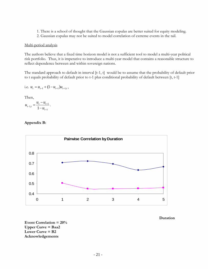
Pairwise Correlation by Duration

0.4

0.5

0.6

0.7

0.8

0 1 2 3 4 5

Duration Event Correlation = 20% Upper Curve = Baa2 Lower Curve = B2 Acknowledgements

- 21 -

The authors would like to express their gratitude and appreciation to the following industry participants for providing valuable historical data and guidance. Ace Global Markets (Ace) Julian Edwards, Steve Capon, and Peter Sprent American International Group (AIG) John Hegeman, John Salinger Beazley GroupAdrian Lewers, Simon Brickman Coface Arnaud Tisseyre, Didier Collet, Xavier Joseph Export Development Corporation (EDC Canada) Norman Kimber EXPORTKREDITNÄMNDEN (ekn) Eva Cassel Hiscox Syndicate Andrew Underwood MIGA (World Bank) Jotaro Hamada Overseas Private Investment Corporation (OPIC) Edith Quintrell, Dr. Stephen Everhart XL Insurance David Wright, Elizabeth Edwards The authors wish to also acknowledge the support and contributions from our colleagues at Willis Re. Ge Zhang made major contributions to the selection of techniques for predictive modeling and Discriminant Function analysis and did the preliminary work on creating a default rates data base. The authors appreciate the efforts from Grace Qiu to continue and expand the database related work started by Ge Zhang. Rick Bowering and Mark Jenkins, Willis Re Political Risk Practice Leaders for North America and Continental Europe, respectively, provided strong support and direction to this project, while David Neckar, Andrew Pace, and James Vickers were generous with their help in the initial phase of gathering data and organizing the project team. The authors are grateful for the time and efforts of Bill Panning, Yves Provencher, Michael Parker, Ian Cook, Jurgen Gaiser-Porter, David Neckar, Ellen Friedman, Peter Szendro, Ron Carlson, and Mark Hvidsten in reviewing the various drafts of this paper and providing valuable feedback.

- 22 -

Finally, we want to express our appreciation for the commitment of Peter Hearn, CEO, Willis Re Inc., and his management team to this project and to long-term research and development at Willis Re. Bibliography

1. Alwis, A., Kremerman, V., Shi, J., (2005): D&O Reinsurance Pricing – A Financial Market Approach, Forum, Casualty Actuarial Society

2. Bohn, J. R. (1999): Characterizing Credit Spreads, Haas School of Business, University of California 3. Das, S., Freed, L., Geng, G., Kapadia, N., (2005): Correlated Default Risk, Santa Clara Univ. 4. Delianedis, G. and Geske, R. (2001) : The component of corporate credit spreads: Default,

Recovery, Tax, Jumps, Liquidity, and Market Factors”, eScholarship Repository, University of California

5. Dhrymes, P. J., (1986): Handbook of Econometrics, Volume III, Elsevier Science Publishers BV 6. Duffie, D., Singleton, K. J. (1999): Modeling Term Structures of Defaultable Bonds, The Review of

Financial Studies, Oxford University Press 7. Duffie, D. and Kenneth, J.S. (2003). Credit Risk: Pricing, Measurement, and Management, chapter 3,

Princeton University Press 8. Embrechts, P., Lindskog, F., McNeil, A., « Modeling Dependence with Copulas and Applications to

Risk Management », In: Handbook of Heavy Tailed Distributions in Finance, ed. S. Rachev, Elsevier, Chapter 8, pp. 329-384 , 2003

9. Finnerty, John D., (2004): Securitizing Political Risk Insurance: Lessons from Past Securitizations, International Political Risk Management – Exploring New Frontiers, MIGA, The World Bank Group

10. Glasserman, P. (2003): Tail Approximations for Portfolio Credit Risk, Columbia Business School 11. Griliches, Z., Intriligator, M.D. (1986). Handbook of Econometrics, Volume III, chapter 27, Elsevier

Science Publishers BV 12. Hamada, J., Haugerudbraaten, H., Hickman, A., Khaykin, I., (2004): Pricing Political Risk within an

Economic Capital Framework. Chapter 14, Country and Political Risk edited by Sam Wilkin, London Risk Books

13. Li, Davis X. (1999): On Default Correlation: A Copula Function Approach. The RiskMetrics Group, Working Paper Number 99-07

14. Lindskog, F., (2000):Modeling Dependence with Copulas and Applications to Risk Management, Swiss Federal Institute of Technology Zurich

15. Lennox, C. (1999). “Identifying Falling Companies: A Re-Evaluation of the Logit, Probit, and DA Approaches,” Journal of Economics and Business 51: 347-364.

16. Lubochinsky, C. (2002): “How much credit should be given to credit spreads”, Financial Stability Review

17. Merton, R. C. (1974): On Pricing of Corporate Debt: The Risk Structure of Interest Rates, Journal of Finance, 29, pp. 449-470

18. Mina, J. (2001): Mark-to-Market, Oversight, and Sensitivity Analysis of CDO’s, Risk Metrics Group 19. Nelsen, R. B.(1999): “Introduction to Copulas”, Springer-Verlag Telos, 20. Pugachevsky, D. (2002): Correlations in Multi-Credit Models. 5th Columbia-JAFEE Conference on

Mathematics in Finance, 5-6 April 2002 21. Ramsey, F.L. and Schafer, D.W. (1997). The Statistical Sleuth: A Course in Methods of Data Analysis,

chapter 21, Duxbury

- 23 -

22. Rebonato, R., Jackel, P. (1999): The Most General Methodology to Create a Valid Correlation Matrix for Risk Management and Option Pricing Purposes. Quantitative Research Centre of the NatWest Group.

23. Rogge, E., Schonbucher, P. J. (2003): Modeling Dynamic Portfolio Credit Risk, Department of Mathematics, Imperial College and ABN AMRO Bank, London and Department of Mathematics, ETH Zurich, Zurich

24. Schonbucher, P. J. (2001): Factor Models – Portfolio credit risks when defaults are correlated, Journal of Risk Finance

25. Sklar, A.(1973): Random Variables, Joint Distribution Functions and Copulas, Kybernetika 26. Wang, S. S. (2002): A Universal Framework for Pricing Financial and Insurance Risks, ASTIN

Bulletin

Glossary Copula A function that joins univariate distribution functions to form multivariate distribution functions. A copula of a multivariate distribution can be thought of as the instrument that describes the dependence structure. Credit Risk is the risk due to uncertainty in a counterparty's (also called an obligor or credit's) ability to meet it’s obligations. Because there are many types of counterparties, from individuals to sovereign governments and many different types of obligations, from auto loans to derivatives transactions, credit risk takes many forms Credit Spread for a bond equals to difference between yield on a risky bond and yield on a default-free government bond with a similar maturity Recovery Rate In the event of a default, the recovery rate is the fraction of the exposure that may be recovered through bankruptcy proceedings or some other form of settlement Biographies of Authors Athula Alwis is Senior Vice President, Global Credit Analytics at Willis Re Inc. in New York City, New York. Athula provides analytical and risk management services to Willis Re clients worldwide for credit, D&O, political risk, surety and other financial products lines of business. Athula is the practice leader for credit analytics at Willis Re Inc. Athula has a BS (First Class Honours) in Mathematics from University of Colombo, Sri Lanka and a MS in Mathematics from Syracuse University, New York. He is an Associate of the Casualty Actuarial Society (CAS) and a member of the American Academy of Actuaries (AAA). Athula is a member of the AAA Risk Based Capital committee, and is a frequent presenter at industry conferences.

- 24 -

Athula co-authored actuarial papers titled “Credit & Surety Pricing and the Effects of Financial Market Convergence” in 2002 and “D&O Reinsurance Pricing – A Financial Market Approach” in 2005. Vladimir Kremerman is Assistant Vice President, Analytical Services at Willis Re Inc. in New York City, New York. He is responsible for property/casualty and specialty lines reinsurance analysis. Vladimir has a Ph.D. in Physics from Vilnius State University. He worked as a physicist at Semiconductor Physics Institute of Lithuanian Academy of Sciences, and Center for Ultrafast Photonics in City University, New York. He authored/coauthored numerous papers on statistical mechanics and an actuarial call paper on D&O Reinsurance Pricing. Junning Shi is Senior Vice President, Analytical Services at Willis Re Inc. in New York City, New York. He provides actuarial consulting services in specialty lines such as marine, aviation, surety, international & retro as well as in many other property & casualty lines. Junning has a Doctor of Arts in Mathematics from Idaho State University. He is a Fellow of the Casualty Actuarial Society (CAS) and a member of the American Academy of Actuaries (AAA). He has authored/co-authored several papers on approximation theory and an actuarial call paper on D&O Reinsurance Pricing. Jason Harger is an actuarial analyst in the Analytical Services Division at Willis Re Inc. in New York City, New York. He provides actuarial consulting services in specialty lines as well as property & casualty lines. Jason has a BS in Operations Research and Industrial Engineering from Cornell University, Ithaca, New York. Yakov Lantsman joined Willis in 2005 as a Senior Vice President responsible for product development. Prior to joining Willis, Yakov, as head of FRM Quantitative Services at Fitch Risk Management Services, provided quantitative support for FitchRisk Advisory Group which offers strategic risk management consulting to leading financial services companies globally. From 1997-2000 Yakov was with Guy Carpenter & Company, Inc. where his responsibilities included performing research and statistical modeling on the key issues of Dynamic Financial Analysis (DFA), a process of modeling the future financial performance of an insurance company. Yakov was a Consulting Statistician from 1992-1997 for Tillinghast with Towers Perrin Company where he developed and delivered statistical modeling consultancy projects for Property/Casualty Division of Tillinghast. From 1984-1991,Yakov was a Senior Researcher at the Tashkent Research Center for Development and Support Industry, Department of Mathematics and Marketing, in Tashkent, Uzbekistan.

- 25 -