Polling Systems - Faculteit Wiskunde en Informaticasem/Tutorial/lecturenotes.pdf · 3 Polling systems with zero and non-zero switch-over times 23 ... and then the central computer

Polling Systems

Performance 2010 Tutorial

November 2010

ii

Contents

1 Introduction 1

1.1 Background and motivation . . . . . . . . . . . . . . . . . . . . . . . . . . . 11.2 Applications of polling models . . . . . . . . . . . . . . . . . . . . . . . . . . 21.3 Model description . . . . . . . . . . . . . . . . . . . . . . . . . . . . . . . . . 31.4 Analysis of polling systems . . . . . . . . . . . . . . . . . . . . . . . . . . . 81.5 Optimization of polling systems . . . . . . . . . . . . . . . . . . . . . . . . . 13

2 Decomposition properties and pseudo-conservation laws in polling mod-

els 17

2.1 Introduction . . . . . . . . . . . . . . . . . . . . . . . . . . . . . . . . . . . . 172.2 Queue length decomposition . . . . . . . . . . . . . . . . . . . . . . . . . . . 182.3 Work decomposition . . . . . . . . . . . . . . . . . . . . . . . . . . . . . . . 21

3 Polling systems with zero and non-zero switch-over times 23

3.1 Introduction . . . . . . . . . . . . . . . . . . . . . . . . . . . . . . . . . . . . 233.2 Model description . . . . . . . . . . . . . . . . . . . . . . . . . . . . . . . . . 243.3 The joint queue length distribution at various epochs . . . . . . . . . . . . . 253.4 The joint queue length distribution at polling epochs . . . . . . . . . . . . . 273.5 Marginal queue lengths and waiting times . . . . . . . . . . . . . . . . . . . 313.6 Computational aspects . . . . . . . . . . . . . . . . . . . . . . . . . . . . . . 32

Bibliography 37

iii

iv CONTENTS

Chapter 1

Introduction

1.1 Background and motivation

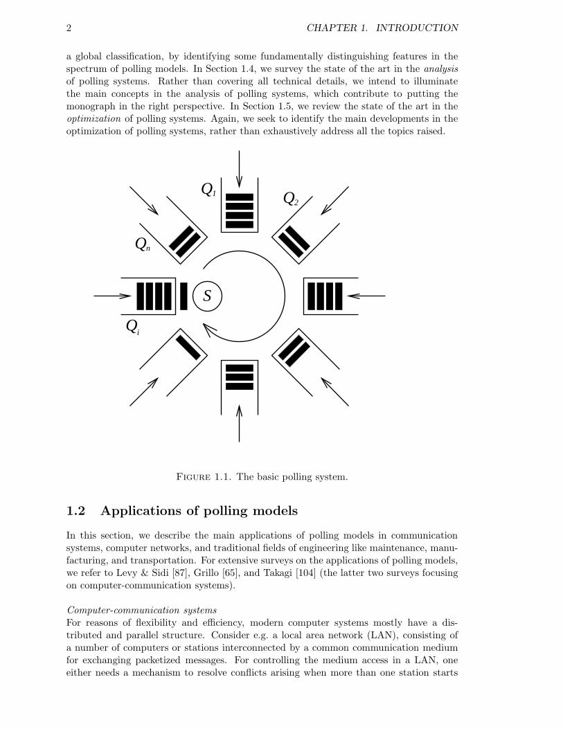
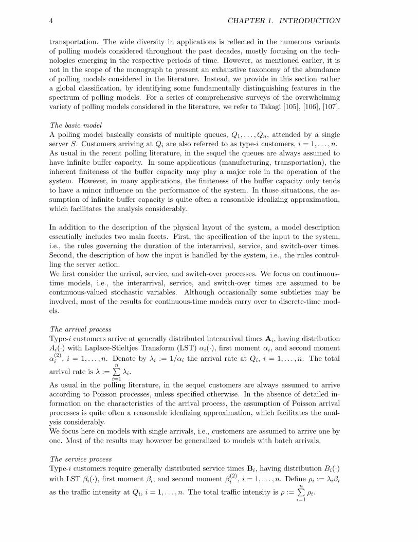
The classical model in queueing theory consists of a single queue attended by a singleserver. Single-server single-queue models have been studied extensively in the literature,cf. Cohen [36] for a rigorous treatment of the main analytical results. In several situa-tions, the traditional single-server single-queue models have proven to be very successfulin accurately predicting waiting times, queue lengths, and buffer overflow probabilities.However, in most of the recent applications, the parallel or distributed character of theservice facilities involves queueing models with multiple servers, multiple queues, or both.This monograph is primarily devoted to queueing models with multiple queues attended bya single server, visiting the queues one at a time, cf. Figure 1.1. Moving from one queue toanother, the server typically incurs a non-negligible switch-over time. Such single-servermultiple-queue models are commonly referred to as polling models. The term ‘polling’originates from the polling data link control scheme, in which a central computer cycli-cally polls the terminals on a communication link to inquire whether they have any datato transmit. When a terminal completes the transmission of data, the data link may beused for some system overhead, and then the central computer polls the next terminal. Inthe associated polling model, the server represents the central computer, the queues cor-respond to the terminals, the customers represent the messages, and the switch-over timecorresponds to the system overhead. In a broader perspective, polling models may arise insituations, in which there are multiple customer classes sharing a common resource, whichis available to only one customer class at a time. In those situations, changing from onecustomer class to another usually involves a non-negligible overhead.Stimulated by a wide variety of applications, polling models have been extensively studiedin the literature, cf. Takagi [105], [106], [107] for a series of comprehensive surveys. In thismonograph, we provide an overview the main exact results available for polling models,in particular focusing on so-called pseudo-conservation laws for the mean waiting timesand the queue length and waiting-time distributions for a class of service disciplines witha certain branching process property, present a detailed analysis of various extensions,and discuss several optimization issues. The remainder of the chapter is organized asfollows. In Section 1.2, we describe the main applications of polling models in communi-cation systems, computer networks, and traditional fields of engineering like maintenance,manufacturing, and transportation. The wide diversity in applications is reflected in thenumerous variants of polling models considered throughout the past decades, mostly fo-cusing on the technologies emerging in the respective periods of time. It is however notin the scope of the monograph to present an encyclopedic categorization of the plethoraof polling models considered in the literature. Instead, in Section 1.3, we provide rather

1

2 CHAPTER 1. INTRODUCTION

a global classification, by identifying some fundamentally distinguishing features in thespectrum of polling models. In Section 1.4, we survey the state of the art in the analysisof polling systems. Rather than covering all technical details, we intend to illuminatethe main concepts in the analysis of polling systems, which contribute to putting themonograph in the right perspective. In Section 1.5, we review the state of the art in theoptimization of polling systems. Again, we seek to identify the main developments in theoptimization of polling systems, rather than exhaustively address all the topics raised.

S

1QQ2

Qn

Qi

Figure 1.1. The basic polling system.

1.2 Applications of polling models

In this section, we describe the main applications of polling models in communicationsystems, computer networks, and traditional fields of engineering like maintenance, manu-facturing, and transportation. For extensive surveys on the applications of polling models,we refer to Levy & Sidi [87], Grillo [65], and Takagi [104] (the latter two surveys focusingon computer-communication systems).

Computer-communication systemsFor reasons of flexibility and efficiency, modern computer systems mostly have a dis-tributed and parallel structure. Consider e.g. a local area network (LAN), consisting ofa number of computers or stations interconnected by a common communication mediumfor exchanging packetized messages. For controlling the medium access in a LAN, oneeither needs a mechanism to resolve conflicts arising when more than one station starts

1.3. MODEL DESCRIPTION 3

to transmit simultaneously, or one needs a protocol to avoid such conflicts, by giving onlyone station at a time permission to transmit data packets. The performance evaluationof the latter category, the so-called conflict-free medium access mechanisms, has greatlystimulated the research in the area of polling models. Adopting the polling terminology,the server represents the right of transmission, the queues correspond to the stations,and the customers represent the data packets. In practice, several versions of conflict-freemedium access protocols are known.One variant is the token ring, i.e., there is an explicit or implicit token circulating on thecommunication ring, representing the right of transmission. When a station receives thetoken, it may start transmitting packets. As soon as the station finishes transmitting, itpasses the token to the next station. So holding the token corresponds to utilizing theserver.Another variant is the slotted ring, i.e., the communication ring is subdivided into timeslots of the size of a single packet, circulating at constant speed. When a station sees anempty slot pass by, it may put a packet in it. In case of destination release the receivingstation subsequently removes the packet from the slot, while in case of source release thetransmitting station empties the slot again. So occupying a slot corresponds to utilizinga server.A slotted ring may be viewed as a multiple-server polling system (unless there is only asingle slot). A token ring is in fact a single-server polling system, but the stations mayhappen to be interconnected by multiple token rings rather than only a single token ring.

Maintenance, manufacturing, transportationIn the first polling study that appeared in the open literature, Mack, Murphy, & Webb[90] considered a situation in which a patrolling repairman cyclically inspects a numberof machines, checks whether or not a failure occurred, if so repairs the machine, and thenmoves to the next machine. In the associated polling model, the server represents therepairman, the queues correspond to the machines, and the customers represent the possi-ble breakdowns. Konigsberg & Mamer [78] studied a similar model, in which an operatorat a fixed position serves a number of storage locations on a rotating carousel conveyor.Models with several independent rotating carousels have also been considered, cf. Kim &Konigsberg [75], Bunday & El-Badri [32].There are also various applications in manufacturing environments. Consider e.g. a flexi-ble manufacturing system, in which a machine periodically changes over from performingone type of operations to another. Here the server represents the machine and the queuescorrespond to the various types of operations. A similar application is multi-product eco-nomic lot scheduling, cf. Sarkar & Zangwill [96].Furthermore, there are applications in transportation networks. Consider e.g. a materialhandling system, in which a vehicle transfers loads from one machining center to another,cf. Bozer [28]. Here the server represents the vehicle, the queues correspond to the ma-chining centers, and the customers represent the loads. Similar applications are publictransport systems, mail delivery, and elevator facilities, cf. Gamse & Newell [61], [62].A last application that is worth mentioning is the control of traffic lights. In polling terms,the stream that is being given green light corresponds to the queue receiving service.

1.3 Model description

As described in the previous section, polling models find a variety of applications in com-munication systems, computer networks, and fields like maintenance, manufacturing, and


transportation. The wide diversity in applications is reflected in the numerous variantsof polling models considered throughout the past decades, mostly focusing on the tech-nologies emerging in the respective periods of time. However, as mentioned earlier, it isnot in the scope of the monograph to present an exhaustive taxonomy of the abundanceof polling models considered in the literature. Instead, we provide in this section rathera global classification, by identifying some fundamentally distinguishing features in thespectrum of polling models. For a series of comprehensive surveys of the overwhelmingvariety of polling models considered in the literature, we refer to Takagi [105], [106], [107].

The basic modelA polling model basically consists of multiple queues, Q1, . . . , Qn, attended by a singleserver S. Customers arriving at Qi are also referred to as type-i customers, i = 1, . . . , n.As usual in the recent polling literature, in the sequel the queues are always assumed tohave infinite buffer capacity. In some applications (manufacturing, transportation), theinherent finiteness of the buffer capacity may play a major role in the operation of thesystem. However, in many applications, the finiteness of the buffer capacity only tendsto have a minor influence on the performance of the system. In those situations, the as-sumption of infinite buffer capacity is quite often a reasonable idealizing approximation,which facilitates the analysis considerably.

In addition to the description of the physical layout of the system, a model descriptionessentially includes two main facets. First, the specification of the input to the system,i.e., the rules governing the duration of the interarrival, service, and switch-over times.Second, the description of how the input is handled by the system, i.e., the rules control-ling the server action.We first consider the arrival, service, and switch-over processes. We focus on continuous-time models, i.e., the interarrival, service, and switch-over times are assumed to becontinuous-valued stochastic variables. Although occasionally some subtleties may beinvolved, most of the results for continuous-time models carry over to discrete-time mod-els.

The arrival processType-i customers arrive at generally distributed interarrival times Ai, having distributionAi(·) with Laplace-Stieltjes Transform (LST) αi(·), first moment αi, and second moment

α(2)i , i = 1, . . . , n. Denote by λi := 1/αi the arrival rate at Qi, i = 1, . . . , n. The total

arrival rate is λ :=n∑

i=1λi.

As usual in the polling literature, in the sequel customers are always assumed to arriveaccording to Poisson processes, unless specified otherwise. In the absence of detailed in-formation on the characteristics of the arrival process, the assumption of Poisson arrivalprocesses is quite often a reasonable idealizing approximation, which facilitates the anal-ysis considerably.We focus here on models with single arrivals, i.e., customers are assumed to arrive one byone. Most of the results may however be generalized to models with batch arrivals.

The service processType-i customers require generally distributed service times Bi, having distribution Bi(·)

with LST βi(·), first moment βi, and second moment β(2)i , i = 1, . . . , n. Define ρi := λiβi

as the traffic intensity at Qi, i = 1, . . . , n. The total traffic intensity is ρ :=n∑

i=1ρi.


The switch-over processMoving from Qi to Qj, the server incurs a generally distributed switch-over time Sij ,

having distribution Sij(·) with LST σij(·), first moment sij, and second moment s(2)ij ,

i, j = 1, . . . , n. As usual in the polling literature, in the sequel, switch-over times arealways assumed to depend only on the previous queue visited or the next queue to be vis-ited, i.e., Sij = Si or Sij = Sj, i, j = 1, . . . , n, respectively. Thus, the distribution of the

total switch-over time incurred during a tour along the queues has LST σ(·) :=n∏

i=1σi(·),

first moment s :=n∑

i=1si, and second moment s(2) :=

n∑

i=1

n∑

j=1sisj +

n∑

i=1(s

(2)i − s2i ). To avoid

ambiguity, in the sequel, Si always corresponds to the switch-over time incurred whenswapping out of Qi, unless specified otherwise.

We now consider the rules controlling the server action. A scheduling strategy is a collec-tion of decision instructions for determining the server action at any given time. Occa-sionally, a scheduling strategy will also be referred to as a scheduling discipline, a pollingstrategy, or a polling policy. A scheduling strategy prescribes whether the server S shouldserve (which customer), switch (to which queue), or idle. Those decisions are made basedon some partial knowledge of the state of the system (queue lengths, past arrival patterns),and on past decisions.Although a scheduling strategy in principle may be arbitrarily involved, it mostly decom-poses into three separate control mechanisms, viz.:i. the routing policy: in which order should S serve the queues;ii. the service policy: while at a queue, which number of customers should S serve;iii. the service order: while at a queue, in which order should S serve customers.We now successively describe the main variants of these three control mechanisms.

The routing policyThe routing policy prescribes in which order S should visit the queues. In the tradi-tional cyclic polling model, the server visits the queues in a strictly cyclic order, i.e.,Q1, . . . , Qn, Q1, . . . , Qn, . . . .One obvious generalization of strictly cyclic polling is periodic polling, introduced inKruskal [80] and revisited in Eisenberg [43], Baker & Rubin [6], and Boxma, Groenendijk,& Weststrate [20]. In periodic polling, the server visits the queues in a fixed order, listedin a polling table of some size m, i.e., a vector of length m with components in {1, . . . , n}.An important special case of periodic polling is scan polling or elevator polling, in whichthe server visits the queues in the order Q1, . . . , Qn, Qn, . . . , Q1, . . . . Another specialcase of periodic polling is star polling, in which the server visits the queues in the orderQ1, Q2, Q1, Q3, Q1, . . . , Qn−1, Q1, Qn, . . . .Another natural generalization of strictly cyclic polling is Markovian polling, introducedin Boxma & Weststrate [27]. In Markovian polling, the server visits the queues accordingto a discrete-time Markov chain with state space {1, . . . , n}, i.e., the server is routed fromQi to Qj with probability pij, i, j = 1, . . . , n. A special case of Markovian polling is ran-dom polling, i.e., pij = pj , i, j = 1, . . . , n, analyzed in Kleinrock & Levy [76]. Mixtures ofperiodic polling and Markovian polling are also conceivable.All above policies are static, in the sense that the routing decisions are made independentlyof the state of the system, so that the sequence of the queues visited is also independentof the input sequence to the system. In dynamic policies, the routing decisions are madebased on some partial knowledge of the state of the system (queue lengths, past arrival pat-terns), and on past decisions, e.g., the server may be instructed to serve the longest queue.


Evidently, in principle the performance of the system may improve substantially by usingsuch information in making the routing decisions. However, gathering such informationand implementing a sophisticated routing policy may involve a considerable communi-cation overhead, and complicate the operation of the system significantly. Therefore, inpractice, dynamic policies are not necessarily preferable to static policies.

The service policyWhile at a queue, the service policy (or strategy, or discipline) prescribes which numberof customers S should serve. There are four classical service disciplines.I. Exhaustive service.Under exhaustive service, the server continues to work until the queue becomes empty.Customers that arrive during the course of the visit, are served in the current visit.II. Gated service.Under gated service, S serves only the customers that were present at the start of thevisit. Customers that arrive during the course of the visit, are served in the next visit.III. Limited service.Under k-limited service, the server continues to work until either a prespecified number ofk customers have been served, or the queue becomes empty, whichever occurs first. Thereare two versions of limited service: gated-limited or exhaustive-limited service, dependingon whether or not S only serves the customers that were present at the start of the visit.IV. Decrementing service.Under k-decrementing service, the server continues to work until either there are a pre-specified number of k customers less present than at the start of the visit, or the queuebecomes empty, whichever occurs first. 1-Decrementing service is commonly referred toas semi-exhaustive service.There are also numerous probabilistic hybrids of the four classical service disciplines. Togive a systematic overview, we now define a family of service disciplines which operate asfollows. If there are mi customers present at the start of the visit to Qi, then a (random)number Li(mi) of them qualify for service. Customers arriving during the visit to Qi qual-ify for service with probability pi. The server continues to work until either a (random)number of Ki(mi) customers have been served, or there are no customers left that qualifyfor service, whichever occurs first.Service disciplines with pi = 1 and pi = 0 are frequently referred to as exhaustive-typeand gated-type policies, respectively, cf. Boxma [16], Levy & Sidi [87], Levy, Sidi, &Boxma [88]. Disciplines with Ki(mi) < ∞ (with positive probability) are frequently re-ferred to as limited-type policies. Similarly, disciplines with Li(mi) < ∞ (with positiveprobability) may be viewed as decrementing-type policies.In binomial-type policies, Ki(mi) = ∞ and Li(mi) is binomially distributed with meanmiqi, 0 ≤ qi ≤ 1, cf. Levy [84], [85]. In Bernoulli-type policies, Li(mi) = mi and Ki(mi)is the sum of mi independent identically geometrically distributed random variables eachwith mean 1/(1 − qi), 0 ≤ qi ≤ 1, cf. Resing [94]. In case Ki(mi) is just a single geo-metrically distributed random variable, we obtain ordinary Bernoulli service, introducedin Keilson & Servi [72], [98]. Ordinary Bernoulli service may be used as an emulation ofki-limited service, under which S serves at most ki customers at Qi (taking qi = 1−1/ki).Note that Bernoulli service and ki-limited service coincide for qi = 0 as well as qi = 1.In its turn, ki-limited service is widely used as an approximation of time-limited service,under which the server stays at most for a time Ti at Qi (taking ki ≈ Ti/βi, the exactvalue depending on whether or not service is preempted when the timer expires). Fordeterministic service times, ki-limited service and Ti-limited service even coincide. A sim-ilar discipline is fixed time service, under which the server stays at a queue for a fixed


time, regardless of whether the queue becomes empty in the meanwhile or not. A servicediscipline under which S always serves a fixed number of customers at a queue does notreally make sense, since (for static routing policies) it inherently causes the system to beunstable.All above policies are local, in the sense that the service decisions are made at each ofthe queues in isolation after the start of the visit. Recently, Boxma, Levy, & Yechiali [24]proposed the globally gated service discipline as a modeling approach to reservation mech-anisms like in the cyclic-reservation multiple-access (CRMA) protocol. Under globallygated service, during a visit to Qi, S serves only the customers present at the start of themost recent visit to Q1. As a generalization of ordinary gated and globally gated service,Khamisy, Altman, & Sidi [74] analyzed the synchronized gated service discipline. Undersynchronized gated service, during a visit to Qi, S serves only the customers present atthe start of the most recent visit to a ‘master’ queue Qπ(i) with π(i) ∈ {1, . . . , n}. Syn-chronized versions of other service disciplines than gated, or service disciplines with othergating epochs than at the start of the most recent visit to Qπ(i), e.g. at the completion ofthe most recent visit to Qπ(i), are also conceivable, cf. Bertsekas & Gallager [7], and Lee& Sengupta [82], [83].Although global in nature, even in the latter policies the service decisions depend on thestate of the system through the marginal queue length only. Policies in which the servicedecisions may be based on the joint queue length, have been considered in Hofri & Ross[70], Koole [79], and Liu, Nain, & Towsley [89]. With regard to the pro’s and con’s of suchsophisticated adaptive service policies similar remarks hold as with regard to dynamicversus static routing policies.

The order of serviceWhile at a queue, the order of service prescribes in which order S should serve customers.While the routing policy and the service policy together dictate the global priorities, theservice order determines the local priorities. In the sequel, the order of service is alwaysassumed to be First Come First Served (FCFS), i.e., customers are assumed to be servedin order of arrival. In fact, the service order does neither matter for the queue lengthdistribution nor, by Little’s law, for the mean waiting times, as long as customers enterservice in an order independent of their service times. Of course, the service order doesmatter for the waiting-time distribution. Polling models with local priority rules withinqueues have been considered in Fournier & Rosberg [52], and Shimogawa & Takahashi [99].

The stability conditionFinally, we briefly discuss the conditions for stability. Recently Fricker & Jaıbi [53] rigor-ously proved that for a system with periodic polling a necessary and sufficient conditionfor stability reads

ρ+ maxi=1,...,n

λiR/Mi < 1, (1.1)

where R is the mean total switch-over time incurred during a cycle, i.e., incurred whenpassing through the polling table once, while Mi is the maximum mean number of type-icustomers served during a cycle, i.e., the mean number of type-i customers that would beserved during a cycle, if there were an infinite number of type-i customers present at thestart of the cycle. Here the system is said to be stable, if it admits a stationary regimewith integrable cycle time. A simple traffic balance argument shows that if the system isstable, then the server is working a fraction ρ of the time, so that the mean cycle time is


given by EC = R/(1 − ρ). So if the system is stable (1.1) may be rewritten as

λiR

1 − ρ< Mi, i = 1, . . . , n, (1.2)

saying that the mean number of type-i customers arriving during a cycle is smaller thanthe maximum mean number of type-i customers served during a cycle. As the server isworking a fraction ρi of the time at Qi, the mean total visit time at Qi in a cycle is givenby EVi = ρiEC = ρiR/(1 − ρ), i = 1, . . . , n. The mean total intervisit time at Qi in acycle follows from EIi = EC − EVi = (1 − ρi)R/(1 − ρ), i = 1, . . . , n.Note that if the system is stable, then all the queues are stable. However, even if asystem is unstable a subset of the queues may still be stable. Assuming that the queuesare indexed such that i ≤ j ⇐⇒ λi/Mi ≤ λj/Mj , Fricker & Jaıbi show that the queuesQ1, . . . , Qκ are stable while the queues Qκ+1, . . . , Qn are unstable with κ being defined as

κ := max{i :i∑

j=1

ρj + λi(R+n∑

j=i+1

βjMj)/Mi < 1}.

In other words, whether or not the individual queues are stable depends on the ratio

λi/Mi. The mean cycle time is given by EC = (R +n∑

j=κ+1βjMj)/(1 −

κ∑

j=1ρj). Note that

(1.1) implies κ = n.The quantityMi is determined by the number of visits toQi as specified in the polling tableand the maximum mean number of customers served during a visit to Qi as specified by theservice discipline (possibly different policies at different visits). For ease of presentation,we now focus on the case of strictly cyclic polling, so that R = s, and the quantity Mi isdetermined by the service discipline at Qi only. (The sufficient stability conditions for thecase of strictly cyclic polling were independently established by Altman, Konstantopoulos,& Liu [1] and Georgiadis & Szpankowski [63], using different techniques. The assumptionsin [1] and [63] on the service disciplines are however somewhat restrictive compared to [53].)For service disciplines like exhaustive and gated that do not impose any (probabilistic)restriction on the maximum mean number of customers served, Mi = ∞, so that thestability condition (1.1) reduces to ρ < 1, which has long been stated without formalproof, cf. Eisenberg [43]. For both the exhaustive and gated version of ki-limited service,Mi = ki, so that (1.2) reduces to λis/(1−ρ) < ki, which also has long been stated withoutformal proof, cf. Kuhn [81]. For ki-decrementing service, Mi = ki/(1 − ρi), so that (1.2)reduces to λis(1 − ρi)/(1 − ρ) < ki, i = 1, . . . , n, saying that the mean increase in thenumber of type-i customers during the intervisit time is smaller than the net decreaseduring the visit time.In [54] Fricker & Jaıbi establish the stability condition for models with Markovian polling;cf. also Borovkov & Schassberger [10]. For dynamic scheduling strategies, there are hardlyany results known on the conditions for stability; cf. Schassberger [97] for the case ofgated-limited service.Throughout the monograph, the conditions for stability are assumed to hold. We furtheralways assume the system under consideration to be in steady state.

1.4 Analysis of polling systems

In this section, we survey the state of the art in the analysis of polling systems. Ratherthan covering all technical details, we intend to illuminate the main concepts in the analysisof polling systems, which contribute to putting the monograph in the right perspective.

1.4. ANALYSIS OF POLLING SYSTEMS 9

We refer to Takagi [103] for a thorough monograph on the analysis of polling systems,containing a detailed enumeration of the main results.

In one of the first polling studies, Avi-Itzhak, Maxwell, & Miller [5] study a two-queuemodel with zero switch-over times and alternating priority (i.e. exhaustive service at bothqueues). They obtain the sojourn time distribution by focusing on the system busy period.Takacs [102] derives the waiting-time distribution in the same model by studying theMarkov chain formed by the state of the system embedded at service completion epochs.Using similar techniques, Eisenberg [42] obtains the waiting-time distribution in a two-queue model with non-zero switch-over times, and either alternating priority or strictpriority, in which the server stops switching when the system is empty.Cooper & Murray [39] study a model with an arbitrary number of queues, zero switch-overtimes, strictly cyclic polling, and exhaustive service at each of the queues. They derive thecycle time distribution by analyzing the Markov chain formed by the state of the systemembedded at visit completion epochs. Cooper [40] obtains the waiting-time distributionfor the model, by viewing the queues in isolation as vacation queues, the intervisit periodsconstituting the vacations. The solution method may also be used for a similar modelwith gated service at each of the queues.Eisenberg [43] studies a model with an arbitrary number of queues, non-zero switch-overtimes, periodic polling, and exhaustive service at each of the queues, in which the serverkeeps switching when the system is empty. Eisenberg derives the waiting-time distribution,the marginal queue length distribution, and the joint queue length distribution at pollingepochs by cleverly exploiting four Markov chains, embedded at service and visit beginningsand endings. The solution method may also be used for a similar model with gated serviceat each of the queues. In a recent study [45], Eisenberg shows how an adapted version ofthe method may be applied in case the server stops switching when the system is empty.

Over the years, several methods have been developed for computing the mean waitingtimes at the various queues in strictly cyclic polling systems with either exhaustive orgated service. To be specific, denote by Wi the waiting time of an arbitrary type-icustomer, i.e., the time elapsing from its arrival to the start of its service, i = 1, . . . , n.One method for computing the mean waiting times is the buffer occupancy method, asused by Cooper & Murray [39], Cooper [40], and Eisenberg [43]. As the name suggests,in the buffer occupancy method, the mean waiting times are computed starting from thebuffer occupancy variables Xij , denoting the queue length at Qj at the start of a visit toQi, i, j = 1, . . . , n.Define Fi(z1, . . . , zn) := E(zXi1

1 . . . zXinn ) to be the probability generating function (pgf) of

the joint queue length distribution at the start of a visit to Qi, | zj |≤ 1, j = 1, . . . , n. Thebuffer occupancy method starts with deriving n functional equations, expressing Fi+1(·)into Fi(·), i = 1, . . . , n.The waiting times are related to the buffer occupancy variables as follows, cf. Watson [108].For exhaustive service, writing Xi for Xii, for Re ω ≥ 0,

E(e−ωWi) =(1 − λiβi)ω

ω − λi(1 − βi(ω))

1 − E((1 − ω/λi)Xi)

ωEXi/λi, (1.3)

the first term on the right-hand side representing the waiting-time Laplace-Stieltjes Trans-form (LST) in the corresponding isolated M/G/1 queue of Qi with arrival rate λi andservice time LST βi(·).


For gated service, for Re ω ≥ 0,


ω − λi(1 − βi(ω))

E((βi(ω)Xi) − E((1 − ω/λi)Xi)

(1 − λiβi)ωEXi/λi, (1.4)

the first term on the right-hand side standing again for the waiting-time LST in the cor-responding isolated M/G/1 queue of Qi. In Chapter 2, we will discuss the occurrence ofthat term in greater detail.The above relationships yield expressions for EWi involving f ′i := EXi and f ′′i := E(Xi(Xi−1)) = E(X2

i )−EXi as unknowns. There are explicit expressions available for the first mo-ments EXi; for exhaustive service, EXi = λiEIi = λi(1 − ρi)s/(1 − ρ); for gated service,EXi = λiEC = λis/(1 − ρ). For the second moments E(X2

i ) there are no explicit expres-sions available. However, the functional equations involving Fi(·), i = 1, . . . , n, render aset of n3 linear equations with n3 unknowns E(XijXik). The latter set of equations canbest be solved in an iterative manner, which requires O(n3logρǫ) elementary operations(additions, multiplications), with ǫ denoting the level of accuracy required.Another method for computing the mean waiting times is the station time method, asused in Ferguson & Aminetzah [51]. As the name reflects, in the station time method themean waiting times are computed starting from the station time variables Uj , denotingthe length of the station time at Qj , j = 1, . . . , n. For exhaustive service, the stationtime consists of the visit time plus the preceding switch-over time. For gated service, thestation time is composed of the visit time plus the following switch-over time.Define Θi(ω1, . . . , ωn) := E(e−ω1Ui−1−...−ωnUi−n) (all indices mod n) to be the Laplace-Stieltjes Transform (LST) of the joint station time distribution of the last n visits at thestart of a visit to Qi, Re ωj ≥ 0, j = 1, . . . , n. The station time method starts withestablishing n functional equations expressing Θi+1(·) into Θi(·), i = 1, . . . , n.The waiting times are related to the station time variables as follows. For exhaustiveservice, for Re ω ≥ 0,


ω − λi(1 − βi(ω))

1 − E(e−ωIi)

ωEIi, (1.5)

with Ii denoting the intervisit time at Qi, i.e., Ii = Si−1 + Ui−1 + . . . + Ui−n+1. Notethat (1.3) and (1.5) are equivalent by the fact that for exhaustive service Xi equals thenumber of arrivals at Qi during Ii, i.e., E(zXi) = E(e−λi(1−z)Ii).For gated service, for Re ω ≥ 0,


ω − λi(1 − βi(ω))

E(e−λi(1−βi(ω))Ci) − E(e−ωCi)

(1 − λiβi)ωECi, (1.6)

with Ci denoting the cycle time at Qi, i.e., Ci = Ui−1 + . . . + Ui−n. The equivalence of(1.4) and (1.6) follows from the fact that for gated service Xi equals the number of arrivalsat Qi during Ci, i.e., E(zXi) = E(e−λi(1−z)Ci).The above relationships yield expressions for EWi involving gi = EUi and gij = E(UiUj)(Qi being visited before Qj) as unknowns. There are explicit expressions available forthe means gi; for exhaustive service, gi = si−1 + EVi = si−1 + ρis/(1 − ρ); for gatedservice, gi = EVi + si = ρis/(1 − ρ) + si. For the covariances gij there are no explicitexpressions available. However, the functional equations involving Θi(·), i = 1, . . . , n,induce a set of n2 linear equations with n2 unknowns gij . The latter set of equationscan be solved in an iterative manner, which requires O(n2logρǫ) elementary operations,with ǫ denoting the level of accuracy demanded. A further advantage of the stationtime method in comparison with the buffer occupancy method is that the structure ofthe set of linear equations involved is somewhat simpler. Without explicitly solving it,

1.4. ANALYSIS OF POLLING SYSTEMS 11

Ferguson & Aminetzah observe from the structure of the set of linear equations that the

intensity-weighted sumn∑

i=1ρiEWi yields a relatively simple expression in comparison with

the extremely complicated expressions for the individual mean waiting times themselves,cf. also Watson [108].For exhaustive service,

n∑

i=1

ρiEWi = ρ

n∑

i=1λiβ

(2)i

2(1 − ρ)+ ρ

s(2)

2s+

s

2(1 − ρ)

[

ρ2 −

n∑

i=1

ρ2i

]

. (1.7)

For gated service,

n∑

i=1

ρiEWi = ρ

n∑

i=1λiβ

(2)i

2(1 − ρ)+ ρ

s(2)

2s+

s

2(1 − ρ)

[

ρ2 +n∑

i=1

ρ2i

]

. (1.8)

These relationships for the mean waiting times are commonly referred to as pseudo-conservation laws. In Chapter 2, we will discuss the existence of these pseudo-conservationlaws in greater detail. A disadvantage of the station time method is that, unlike the bufferoccupancy method, it only appears to be applicable to polling systems with either exhaus-tive or gated service.Sarkar & Zangwill [95] describe a refinement of the station time method. They expressthe n2 unknowns gij into the n unknowns gii, and derive a set of n linear equations forthe latter coefficients, which however appears to be less sparse.Konheim & Levy [77] describe a modification of the buffer occupancy method. Theypropose to calculate E(X2

i ) by the so-called descendant set approach, which allows thecomputation of the mean waiting time at a single queue in only O(nlogρǫ) elementaryoperations, with ǫ the level of accuracy desired.Concluding, although efficient numerical evaluation of the mean waiting times is non-trivial, polling systems with exhaustive or gated service do allow an exact analysis forgenerally distributed service times, generally distributed switch-over times, and an arbi-trary number of queues. Polling systems with limited or decrementing service, however,do not allow an exact analysis, apart from some special cases like two-queue cases andcompletely symmetric cases. Eisenberg [44] studies a two-queue model with zero switch-over times and alternating service (i.e. 1-limited service at both queues), transforming theproblem of finding the joint queue length distribution into the problem of solving a singu-lar Fredholm integral equation. Cohen & Boxma [37] analyze the same model, translatingthe problem into a Riemann-Hilbert boundary value problem. Using similar techniques,Boxma [14] studies a symmetric two-queue model with non-zero switch-over times and1-limited service at both queues. Boxma & Groenendijk [18] analyze an asymmetric two-queue model with non-zero switch-over times and 1-limited service at both queues byformulating a Riemann boundary value problem. Cohen [38] considers a two-queue modelwith zero switch-over times and 1-decrementing (semi-exhaustive) service at both queues.The solution of the specific boundary value problem as formulated in each of the latterstudies typically requires an arsenal of most advanced techniques from complex functiontheory, usually rendering contour-integral expressions for the mean waiting times. Forpolling systems with k-limited or k-decrementing service and n > 2 queues, only approx-imative results are available, apart from some mean-value results for global performancemeasures, like the cycle times, or for the waiting times in a completely symmetric system(cf. Fuhrmann [56] for the special case of 1-limited service).Summarizing, we observe a striking difference in complexity between on the one hand


service disciplines, like exhaustive and gated, that can be analyzed exactly in a generalsetting by standard methods, and on the other hand service disciplines, like limited anddecrementing, that can only be analyzed exactly in special cases by most ingenious tech-niques.The existence of such a sharp distinction is illuminated in Resing [94] and independentlyexplained in Fuhrmann [55]. Both Resing and Fuhrmann consider the class of servicedisciplines that satisfy the following property:

Property 1.4.1

If there are ki customers present at Qi at the start of a visit, then during the course ofthe visit, each of these ki customers will effectively be replaced in an i.i.d. manner by arandom population having probability generating function (pgf) hi(z1, . . . , zn), which maybe any n-dimensional pgf.

By using a multi-type branching process approach, both Resing and Fuhrmann show thatthe class of service disciplines that satisfy the above property allows an exact analysis. Theresults of Resing and Fuhrmann suggest that service disciplines that violate Property 1.4.1defy an exact analysis, except for some special cases, like two-queue cases and completelysymmetric cases.The key element in their exposition is that if the service disciplines in a polling systemsatisfy Property 1.4.1, it is possible to relate the pgf Gi(z1, . . . , zn) := E(zYi1

1 . . . zYinn ) of

the joint queue length distribution at the end of a visit to Qi to the pgf Fi(z1, . . . , zn) :=E(zXi1

1 . . . zXinn ) of the joint queue length distribution at the beginning of a visit to Qi by

Gi(z1, . . . , zn) = Fi(z1, . . . , zi−1, hi(z1, . . . , zn), zi+1, . . . , zn). (1.9)

Moreover, it is possible to relate Fi+1(z1, . . . , zn) to Gi(z1, . . . , zn) by

Fi+1(z1, . . . , zn) = Gi(z1, . . . , zn)σi(

n∑

j=1

λj(1 − zj)), (1.10)

irrespective of the service disciplines (ignoring here some subtleties in case the total switch-over time in a cycle is zero, cf. Chapter 3). Thus, we obtain 2n equations for 2n functions,which may be combined to obtain a functional equation for one of the functions Fi(·) orGi(·), which may then be solved by a standard iterative procedure. As we will show inSection 2.1, most of the relevant performance measures like marginal queue lengths at anarbitrary epoch and waiting times may directly be derived from Fi(·) and Gi(·). Note thatthe approach of Resing and Fuhrmann is closely related to the buffer occupancy method,which was outlined earlier in the present section. In fact, the station time method, whichwas also sketched there, only appears to be applicable to a very restricted subclass of theservice disciplines satisfying Property 1.4.1.Assuming the service disciplines to satisfy Property 1.4.1, Resing shows that in case thetotal switch-over time in a cycle is non-zero, the joint queue length process at the pollingepochs of a fixed but arbitrary queue constitutes a multi-type branching process withimmigration in each state. The particle types in the branching process correspond to thecustomer types in the polling model, the offspring in the branching process represents thecustomers arriving during the service times in the polling model, and the immigration inthe branching process corresponds to the customers arriving during the switch-over timesin the polling model. In case the total switch-over time in a cycle is zero, Resing showsthat the joint queue length process at the polling epochs of a fixed queue constitutes amulti-type branching process with immigration in state zero only. The immigration in

1.5. OPTIMIZATION OF POLLING SYSTEMS 13

the branching process then corresponds to the customers arriving to an empty system inthe polling model. So the models with zero and non-zero switch-over times are closelyrelated through a common offspring generation, the only difference originating from theimmigration. In Chapter 3, we expose the relationship between models with zero andnon-zero switch-over times in greater technical detail.The exhaustive service discipline satisfies Property 1.4.1 with hi(z1, . . . , zn) = ηi(

∑

j 6=i

λj(1−

zj)). Here ηi(·) is the LST of the busy-period distribution in an ordinary isolated M/G/1queue with arrival rate λi and service time distribution Bi(·), satisfying the functionalequation ηi(ω) = βi(ω+λi(1−ηi(ω))), cf. [36] p. 250. The gated service discipline satisfies

Property 1.4.1 with hi(z1, . . . , zn) = βi(n∑

j=1λj(1− zj)). Limited and decrementing service

disciplines violate Property 1.4.1, and have indeed not yielded an exact analysis, exceptfor some special cases, like two-queue cases and completely symmetric cases.Models with server-position dependent arrival rates and customer branching (as the wordsuggests) satisfy Property 1.4.1, and may thus be analyzed exactly by using a multi-typebranching process approach. There are also some service disciplines, like synchronizedgated, that strictly speaking do not satisfy Property 1.4.1, but still allow an exact anal-ysis. Most of these service disciplines, however, satisfy the following generalization ofProperty 1.4.1:

Property 1.4.2

If there are ki customers present at Qi at the beginning (or the end) of a visit to Qπ(i), withπ(i) ∈ {1, . . . , n}, then during the course of the visit to Qi, each of these ki customers willeffectively be replaced in an i.i.d. manner by a random population having pgf hi(z1, . . . , zn),which may be any n-dimensional pgf.

1.5 Optimization of polling systems

In this section, we review the state of the art in the optimization of polling systems.As mentioned earlier, we seek to identify the main issues in the optimization of pollingsystems, rather than exhaustively discuss all the achievements made. For extensive sur-veys on optimization of polling systems, we refer to Boxma [16] (static optimization) andYechiali [110] (semi-dynamic optimization).

In most of the polling applications, some degree of freedom exists in the design or con-trol of the system in choosing the parameters of the scheduling discipline (visit order,visit lengths, service order). A major objective in studying polling systems is to developsufficient understanding of how these parameters influence the operation of the system,and how these parameters should thus be chosen so as to improve the performance ofthe system. Nevertheless, compared to the well-trodden area of the analysis of pollingsystems, the field of optimization of polling systems still remains relatively unexplored.Although for example many waiting-time approximations have been proposed for limited-type service policies, the problem of determining appropriate values for the service limitshas hardly been addressed.In the optimization of polling systems, the problem formulation is typically to optimizesome measure of the system performance over some class of feasible scheduling disciplines.So there are two factors that play a role, first, what is the performance measure to beoptimized, second, what is the class of feasible scheduling disciplines.


Concerning the first factor, there is probably no generic comprehensive measure to eval-uate the system performance. Efficiency and fairness are commonly viewed as importantaspects of the system performance. Although it is somewhat unclear exactly how efficiencyand fairness should be defined, it is widely believed that there is some trade-off betweenthem. On the one hand, exhaustive service is considered to be efficient but not very fair, asa heavily-loaded queue may dominate the complete system. On the other hand, 1-limitedservice is considered to be fair, as each of the queues receives at most one service per visit,but not very efficient. Ideally, a performance measure should relate all important aspectsof the system performance to measurable quantities like waiting times, queue lengths, andexcess probabilities, and should indicate how all those aspects weigh against each other. In

view of these considerations,n∑

i=1ciλiEWi (by Little’s law equivalent to

n∑

i=1ciELi, with Li

denoting the number of waiting type-i customers at an arbitrary epoch) is widely acceptedas a reasonable measure of the system performance.Concerning the second factor, usually the class of feasible scheduling disciplines consists ofa family of strategies of a similar structure that differ by some (vectorial) parameter. Wenow successively discuss some optimization studies that focus on optimization of a routingvector (routing probabilities, or polling table), a service vector (service probabilities, orservice limits), and a routing vector and a service vector simultaneously. In addition, wemention some optimization studies that analyze less structured dynamic polling policies.

Optimization of the routing policy for a given service policyA considerable amount of research effort has been devoted to static optimization, i.e., opti-mization of static routing policies, in which the routing decisions are made independentlyof the state of the system. Boxma, Levy, & Weststrate [21] (cf. also [109]) consider asystem with random polling, and at each of the queues either exhaustive or gated service.They address the problem of finding the routing probabilities (p1, . . . , pn) that minimizen∑

i=1ρiEWi, the latter quantity being explicitly known from the pseudo-conservation law

for random polling, cf. [27]. Boxma, Levy, & Weststrate [16] (cf. also [109]) consider a sys-tem with periodic polling and at each of the queues either exhaustive, gated, or 1-limited

service. They study the problem of determining a polling table that minimizesn∑

i=1ρiEWi.

The proposed approach is to use the optimal visit ratios in random polling (i.e. the routingprobabilities (p1, . . . , pn)) as indication for the optimal visit ratios in periodic polling (i.e.the occurrence ratios of the queues in the polling table), and then to use the Golden Ratioprocedure as a heuristic for spacing the visits within the polling table. Boxma, Levy, &Weststrate [23] (cf. also [109]) address the generalized problem of determining a polling

table that minimizesn∑

i=1ciλiEWi, the latter quantity now being approximated in terms

of the occurrence ratios of the queues in the polling table. Kruskal [80] studies a similarproblem with deterministic arrival, service, and switch-over processes. In all cases, theoptimal visit ratios are given by surprisingly simple square-root formulae.Also, a considerable amount of research effort has been put in semi-dynamic optimization,i.e., optimization of semi-dynamic routing policies, in which periodically the visit orderfor some future period is determined, based on some partial knowledge of the state of thesystem. Browne & Yechiali [30] consider a system with either exhaustive or gated serviceat each of the queues. They address the problem of finding the visit order, at the start ofeach cycle, that minimizes the expected duration of the new cycle, based on knowledge ofthe queue lengths. The optimal visit order is given by a remarkably simple index-type rule.However, they do not explicitly indicate how minimization of the expected duration of each

1.5. OPTIMIZATION OF POLLING SYSTEMS 15

new cycle is supposed to contribute to optimizing the system performance, in particularminimizing the mean waiting times. Actually, the mean cycle time remains s/(1 − ρ), cf.[1], in other words, the server is doing nothing but deferring the service of customers tofuture cycles. Results of Fabian & Levy [48] suggest that among all semi-dynamic visitorders, the order that minimizes (maximizes) the expected duration of each new cycle infact yields the largest (smallest) mean waiting times. Purely dynamic optimization of therouting policy (for a given service policy) has hardly received any attention so far.

Optimization of the service policy for a given routing policyBorst, Boxma, & Levy [13] consider a system with a k-limited service strategy at eachof the queues. They address the problem of determining the vector of service limits

(k1, . . . , kn) that minimizesn∑

i=1ciλiEWi. Blanc & Van der Mei [9] study a similar op-

timization problem in a system with a Bernoulli service strategy at each of the queues.Purely dynamic optimization of the service policy (for a given routing policy) has hardlyreceived any attention so far.

Simultaneous optimization of routing policy and service policyBorst, Boxma, Harink, & Huitema [12] consider a system operated with a fixed timepolling (ftp) scheme. An ftp scheme specifies which queue should be visited at what time,i.e., it specifies not only the order of the visits, but also the starting times of the visits.

They address the problem of constructing an ftp scheme that minimizesn∑

i=1ciλiEWi.

Liu, Nain, & Towsley [89] consider a system with a dynamic polling policy, i.e., a col-lection of instructions for making decisions on whether the server S should serve (whichcustomer), switch (to which queue), or idle, based on some partial knowledge of the stateof the system. They attempt to identify policies that stochastically minimize the totalamount of work and the total number of customers present in the system at an arbitraryepoch. They show that optimal policies are exhaustive and greedy, i.e., the server shouldneither idle nor switch when a queue is non-empty. In addition, they show that in asymmetric system, optimal policies are patient, and belong to the class of Stochastically-Largest-Queue policies, i.e., the server should remain idling at the last visited queue whenthe system is empty, and the server should never switch to a queue known to be stochas-tically smaller than another queue.For a model with zero switch-over times, the optimal (non-preemptive) polling policy isknown to be given by the cµ-rule, cf. Meilijson & Yechiali [91], and Buyukkoc, Varaiya, &Walrand [33]. For a symmetric two-queue model with non-zero switch-over times, Hofri& Ross [70] show that the policy that minimizes the sum of discounted switch-over timesand the holding cost, is exhaustive service in a nonempty system, and is of thresholdtype for switching from an empty queue to another. For an asymmetric two-queue modelwith switch-over costs rather than switch-over times, Koole [79] shows that the policythat minimizes the sum of discounted switching cost and holding cost, is not a thresholdpolicy, but that the best threshold policy approaches the optimal policy very well.

Monotonicity issuesClosely related to optimization issues are questions of stochastic ordering or monotonic-ity of the various performance measures with regard to the inducing stochastic processes(arrival process, service process, switch-over process), or with regard to the schedulingdiscipline (routing policy, service policy, order of service).For a fixed but arbitrary routing policy, Levy, Sidi, & Boxma [88] establish a hierarchy

of dominance relations among work-conserving, non-idling service policies with respect tothe total amount of work in the system at any time. Under fairly mild assumptions, theyshow that the closer a service policy approaches the standard exhaustive service policy,the higher the service policy reaches in the hierarchy, so that in particular the standardexhaustive service policy figures at the top of the hierarchy.Altman, Konstantopoulos, & Liu [1] consider a system with strictly cyclic polling, andat each of the queues either exhaustive-type or gated-type service. They show that thequeue lengths at polling epochs, the visit times, the intervisit times, and the cycle timesare stochastically increasing in the arrival rates, the service times, and the switch-overtimes.Note that the above ordering results refer to global performance measures or performancemeasures that are defined at polling epochs. For detailed performance measures like wait-ing times or queue lengths at arbitrary epochs there are hardly any ordering results known.In view of [1], it might be conjectured that also the waiting time and the queue lengthat Qi are stochastically increasing with regard to the arrival rates, the service times, andthe switch-over times as well as the ‘limitedness’ of the service at Qi, but most of thestatements of such tendency have either been disproved by simple counterexamples orhave lacked proof so far.

16

Chapter 2

Decomposition properties and

pseudo-conservation laws in

polling models

2.1 Introduction

Overviewing the recent polling literature, we see a prominent role played by so-calledpseudo-conservation laws, which provide exact expressions for a specific weighted sum of

the mean waiting times, mostlyn∑

i=1ρiEWi, cf. Ferguson & Aminetzah [51], Watson [108].

Although the individual mean waiting times usually involve extremely complicated expres-sions, a pseudo-conservation law typically provides a relatively simple explicit expression,which e.g. depends on the switch-over times only through the first two moments of theirsum. There are even service disciplines, like Bernoulli service, for which the individ-ual mean waiting times are completely unknown, but for which a pseudo-conservationlaw is still explicitly known. Thus, pseudo-conservation laws provide a useful measureof the overall system performance. In addition, pseudo-conservation laws prove to be avaluable instrument for constructing and validating waiting-time approximations, and fordetermining the mean waiting times in a completely symmetric system in a simple manner.Pseudo-conservation-law-based waiting-time approximations for models with 1-limited ser-vice and an arbitrary number of queues are developed e.g. in Boxma & Meister [25], [26],Groenendijk [66], Srinivasan [100]. Waiting-time approximations for similar models withk-limited service are presented e.g. in Chang & Sandhu [34], Everitt [46], [47], Fuhrmann& Wang [60].The existence of pseudo-conservation laws is interpreted in Boxma & Groenendijk [17],and further clarified in Boxma [15]. The framework presented by Boxma & Groenendijkunified and generalized the pseudo-conservation laws existing until then, and also ex-plained why they existed. In addition, the approach allows a relatively simple derivationof pseudo-conservation laws, and a probabilistic interpretation of the various terms occur-ring in pseudo-conservation laws. Until then, pseudo-conservation laws were obtained bycumbersome ad hoc methods, which did not really explain why they existed, and whatthe various terms occurring represented.The key element in the framework presented by Boxma & Groenendijk is the property ofwork decomposition, which builds on the fundamental property of work conservation, andis closely related to the concept of queue length decomposition, as described in Fuhrmann& Cooper [59]. To illuminate these concepts, we consider in the present chapter a single-

17

18CHAPTER 2. DECOMPOSITION PROPERTIES AND PSEUDO-CONSERVATION LAWS IN POLLING MODELS

server queueing system, not necessarily a polling model, with a Poisson arrival processof rate λ, a service time distribution B(·) with LST β(·) and mean β, and service inter-ruptions. The service interruptions are assumed to result from some kind of interferingprocess that from time to time may keep the server from working, even when there arecustomers present. A period during which the server is not working, because of a serviceinterruption, or because there are no customers present, will be referred to as a non-servinginterval.The service interruptions may be interwoven with the arrival and service process in anarbitrarily complex manner, but may not anticipate on the arrival and service times of fu-ture customers. In particular, the durations of successive service interruptions are allowedto be dependent.For now, we abstract from what kind of interfering process causes the service interruptions.In a performability setting, a service interruption typically represents a down-period of thesystem. In the context of polling models, a service interruption usually corresponds to aswitch-over time, or to an intervisit period with regard to a specific queue, depending uponwhether the polling system in totality is viewed as a system with service interruptions, orjust a specific queue in isolation. Broadening the scope, the service interruptions may alsorepresent set-up times, shut-down times, reconfiguration times, periods during which theserver performs some secondary tasks.The remainder of the chapter is organized as follows. In Section 2.2, we describe theproperty of queue length decomposition for the model under consideration. Focusing ona specific queue in a polling system in isolation, we indicate how the queue length decom-position also translates into a decomposition of the waiting time, as already recognized inSection 1.4, cf. (1.3), (1.4), (1.5), (1.6). In Section 2.3, we elaborate on the related prop-erty of work decomposition. Applying it to a polling system in totality, we sketch howthe work decomposition property leads to pseudo-conservation laws for the mean waitingtimes, as already observed in Section 1.4, cf. (1.7), (1.8).

2.2 Queue length decomposition

Using concepts from the theory of branching processes, under rather mild assumptions,Fuhrmann & Cooper [59] prove the following queue length decomposition property for themodel under consideration:

Nd= NM/G/1 + NI , (2.1)

withd= denoting equality in distribution;

N := the queue length at an arbitrary epoch;NM/G/1 := the queue length at an arbitrary epoch in the ‘corresponding’ M/G/1 system;NI := the queue length at an arbitrary epoch in a non-serving interval;NM/G/1 and NI being independent.The corresponding M/G/1 system is an ordinary M/G/1 queue with similar traffic char-acteristics, but without any service interruptions. To find the distribution of N, it thussuffices to find the distribution of NI , as the distribution of NM/G/1 is simply known fromthe Pollaczek-Khintchine formula, cf. [36] p. 238. From a methodological point of view,however, it is usually preferable to analyze the queue length at the beginning and the endof a non-serving interval rather than to study NI , the queue length at an arbitrary epochin a non-serving interval. Therefore, we now relate the distribution of NI to the queue

length distribution at such embedded epochs. Denote by N(k)begin and N

(k)end the queue length

2.2. QUEUE LENGTH DECOMPOSITION 19

at the beginning and the end of the k-th non-serving interval. Denote by Nbegin and Nend

a pair of stochastic variables with as joint distribution the stationary joint distribution of

N(k)begin and N

(k)end.

Lemma 2.2.1

Pr{NI = l} =Pr{Nbegin ≤ l} − Pr{Nend ≤ l}

ENend − ENbegin. (2.2)

Written in terms of pgf’s,

E(zNI ) =E(zNbegin) − E(zNend)

(1 − z)(ENend − ENbegin), | z | ≤ 1. (2.3)

Proof

Because of the PASTA property, NI has the same distribution as the number of customersseen by an arbitrary customer arriving in a non-serving interval. In the first K non-servingintervals, the fraction of customers that see l customers upon arrival is

K∑

k=1

I{N

(k)begin≤l≤N

(k)end−1}

K∑

k=1

(N(k)end − N

(k)begin)

,

with I{E} denoting the indicator function of the event E. So, using the law of largenumbers,

Pr{NI = l} = limK→∞

K∑

k=1

I{N

(k)begin≤l≤N

(k)end−1}

/K

K∑

k=1

(N(k)end − N

(k)begin)/K

=Pr{Nbegin ≤ l ≤ Nend − 1}

ENend − ENbegin

=Pr{Nbegin ≤ l} − Pr{Nend ≤ l}

ENend − ENbegin,

as Pr{Nbegin ≤ Nend} = 1.�

The queue length decomposition property (2.1) only holds if the order of service is in-dependent of the service times. Consequently, it typically does not hold for a pollingsystem in totality, but it does hold for each of the queues in isolation, assuming that theorder of service at each of the queues is independent of the service times. Therefore, wenow focus on the queue length at a specific queue in a polling system in isolation, let ussay Qi. For the specification of the arrival, service, and switch-over processes, we refer tothe description of the ‘basic model’ in Section 1.3. The queue length Nbegin and Nend atthe beginning and the end of a non-serving interval then correspond to the queue lengthYi at the end and Xi at the beginning of a visit to Qi, respectively. Applying (2.1) and(2.3) to Qi, we then obtain

Nid= Ni|M/G/1 + Ni|I , (2.4)

20CHAPTER 2. DECOMPOSITION PROPERTIES AND PSEUDO-CONSERVATION LAWS IN POLLING MODELS

E(zNi|I ) =E(zYi) − E(zXi)

(1 − z)(EXi − EYi), | z | ≤ 1, (2.5)

withNi := the queue length at Qi at an arbitrary epoch;Ni|M/G/1 := the queue length at an arbitrary epoch in the ‘corresponding’ M/G/1 queueof Qi in isolation;Ni|I := the queue length at Qi at an arbitrary epoch in an intervisit period; Ni|M/G/1 andNi|I being independent.By (2.4) and (2.5), to find the queue length distribution at Qi at an arbitrary epoch itsuffices to find the queue length distribution at Qi at the beginning and the end of avisit, respectively. Note that for the class of service disciplines that satisfy Property 1.4.1,E(zXi) = Fi(1, . . . , 1, z, 1, . . . , 1) and E(zYi) = Gi(1, . . . , 1, z, 1, . . . , 1), with z as i-th ar-gument, are actually known.We now abstract from the polling context again. If the order of service in the system withservice interruptions is FCFS, then the sojourn time R of an arbitrary customer, i.e., thetime from its arrival to the completion of its service, is related to the queue length N

(the total number of customers present, including a customer possibly in service) at anarbitrary epoch by the distributional form of Little’s law, cf. Keilson & Servi [73]:

E(zN) = E(e−λ(1−z)R), | z | ≤ 1, (2.6)

provided the sojourn time of customers is independent of arrivals after their own arrival.Similarly, the waiting time W of an arbitrary customer is related to the number L ofwaiting customers (excluding a customer possibly in service):

E(zL) = E(e−λ(1−z)W), | z | ≤ 1. (2.7)

Taking expectations in either (2.6) or (2.7) yields the original form of Little’s law. Com-bining (2.1) and (2.6), taking λ(1 − z) = ω, we obtain the following sojourn time decom-position:

E(e−ωR) = E(e−ωRM/G/1)E((1 − ω/λ)NI ), Re ω ≥ 0, (2.8)

with RM/G/1 denoting the sojourn time of an arbitrary customer in the correspondingM/G/1 system.Noting that E(e−ωR) = E(e−ωW)β(ω), we obtain from (2.8) the following waiting-timedecomposition:

E(e−ωW) = E(e−ωWM/G/1)E((1 − ω/λ)NI ), Re ω ≥ 0, (2.9)

with WM/G/1 denoting the waiting time of an arbitrary customer in the correspondingM/G/1 system.We now return to the polling setting again. Since the order of service is required to beFCFS here, the properties (2.6)-(2.9) do not hold for a polling system in totality, but theydo hold for a specific queue in isolation with FCFS order of service. Applying (2.9) to Qi,using (2.5) and the Pollaczek-Khintchine formula, cf. [36] p. 255, we obtain


ω − λi(1 − βi(ω))

E((1 − ω/λi)Yi) − E((1 − ω/λi)

Xi)

(EXi − EYi)ω/λi.

Taking for exhaustive service Yi ≡ 0 and E(zXi) = E(e−λi(1−z)Ii) leads to (1.3) and (1.5).Noting that for gated service E(zYi) = E(βi(λi(1 − z))Xi) and E(zXi) = E(e−λi(1−z)Ci)gives (1.4) and (1.6).

2.3. WORK DECOMPOSITION 21

2.3 Work decomposition

In the previous section, we described the property of queue length decomposition, andindicated how it also translates into a decomposition of the waiting times at the individualqueues in a polling system. In this section, we focus on the related property of workdecomposition, and sketch how it leads to pseudo-conservation laws for the mean waitingtimes in a polling system, as shown by Boxma & Groenendijk [17].Adapting the arguments of Fuhrmann & Cooper, under even milder assumptions, Boxma& Groenendijk prove the following work decomposition property for the model underconsideration:

Vd= VM/G/1 + VI , (2.10)

withV := the amount of work in the system at an arbitrary epoch;VM/G/1 := the amount of work at an arbitrary epoch in the correspondingM/G/1 system;VI := the amount of work in the system at an arbitrary epoch in a non-serving interval;VM/G/1 and VI being independent.When the amount of work in a non-serving interval were always zero, i.e., VI ≡ 0, (2.10)would reduce to the fundamental property of work conservation, which in fact holds evenin sample-path sense. Note that in a polling system it is generally not the case thatVI ≡ 0, since the server may be switching when there are customers present.The work decomposition property still holds if the order of service is not independent ofthe service times, reflecting that in a sense the amount of work in the system is a lesssensitive quantity than the queue length. Consequently, it holds in particular for the totalamount of work in a polling system. Therefore, we now focus on the total amount of workin a polling system, and show how the work decomposition property leads to a pseudo-conservation law for the mean waiting times. For the specification of the arrival, service,and switch-over processes, we refer to the description of the ‘basic model’ in Section 1.3.Applying Brumelle’s formula [31],

EV =n∑

i=1

ρiEWi +1

2

n∑

i=1

λiβ(2)i . (2.11)

From the Pollaczek-Khintchine formula, cf. [36] p. 255,

EVM/G/1 =

n∑

i=1λiβ

(2)i

2(1 − ρ). (2.12)

Taking expectations in (2.10), substituting (2.11), (2.12), we obtain the following relation-ship for the mean waiting times:

n∑

i=1

ρiEWi = ρ

n∑

i=1λiβ

(2)i

2(1 − ρ)+ EVI . (2.13)

When the amount of work in a non-serving interval were always zero, i.e., EVI = 0, (2.13)

would reduce to the property thatn∑

i=1ρiEWi does not depend on the scheduling discipline

as long as EVI = 0, which is commonly referred to as a conservation law.

For strictly cyclic polling, Boxma & Groenendijk [17] show that EVI may be determinedas follows:

EVI = ρs(2)

2s+

s

2(1 − ρ)

[

ρ2 −

n∑

i=1

ρ2i

]

+

n∑

i=1

EZii, (2.14)

with Zii denoting the amount of work left behind by the server at Qi at the completionof a visit.Substituting (2.14) into (2.13), we obtain the following relationship for the mean waitingtimes:

n∑

i=1

ρiEWi = ρ

n∑

i=1λiβ

(2)i

2(1 − ρ)+ ρ

s(2)

2s+

s

2(1 − ρ)

[

ρ2 −n∑

i=1

ρ2i

]

+n∑

i=1

EZii, (2.15)

which is commonly referred to as a pseudo-conservation law, sincen∑

i=1ρiEWi now does

depend on the scheduling discipline through the terms EZii. As a pleasing circumstancehowever, EZii is determined by the service discipline at Qi only, i.e., not by the servicediscipline at Qj, j 6= i, e.g. [17]:I. Exhaustive service:

EZii = 0.

II. Gated service:

EZii =ρ2

i s

1 − ρ.

III. 1-Limited service:

EZii =ρ2

i s

1 − ρ+ ρi

λis

1 − ρEWi.

IV. 1-Decrementing service:

EZii = −ρ2

i λ2iβ

(2)i s

2(1 − ρ)+ ρi

λi(1 − ρi)s

1 − ρEWi.

Substituting the above expressions into (2.15) yields the pseudo-conservation laws, whichbefore were only known to hold in cases with the same service disciplines at each of thequeues.Here we sketched the derivation of a pseudo-conservation law for a continuous-time modelwith strictly cyclic polling and single Poisson arrivals. Without seriously complicatingthe derivation, continuous-time may be replaced by discrete-time, cf. [19], strictly cyclicpolling may be generalized to periodic polling, cf. [20], or Markovian polling, cf. [27], andsingle Poisson arrivals may be generalized to batch Poisson arrivals, cf. [15].

22

Chapter 3

Polling systems with zero and

non-zero switch-over times

3.1 Introduction

In the present chapter, we consider two different single-server polling systems: (i) a modelwith zero switch-over times, and (ii) a model with non-zero switch-over times, in which theserver keeps cycling when the system is empty. For both models, we relate the steady-statequeue length distribution at a queue to the queue length distribution at visit beginningand visit completion instants at that queue. As a by-product, we obtain a shorter proof ofthe Fuhrmann-Cooper decomposition, discussed earlier in Section 2.2. For the importantclass of service disciplines with a branching structure satisfying Property 1.4.1, we exposea strong relationship between both the queue length and the waiting-time distribution inthe two models. We also show how the latter relationship can be exploited to reduce thecomputational complexity of numerical moment calculations.As described in Section 2.1, polling systems may be viewed as queueing systems withservice interruptions. Focusing on a specific queue in isolation, the service interruptionscorrespond to the intervisit times of the server with regard to that queue. Accordingly,the concept of queue length decomposition for queues with service interruptions (cf. Equa-tion (2.1), Fuhrmann & Cooper [59]) has proven to be very fruitful for the analysis ofpolling models. It has also led to the concept of work decomposition in polling mod-els (cf. Equation (2.10), Boxma [15]), which relates the amount of work in a system withswitch-over times to the amount of work in a system with similar traffic characteristics butwithout switch-over times. Note that in the latter case, the switch-over times constitutethe service interruptions. Heretofore, models with switch-over times and models withoutswitch-over times had usually been treated separately, often via different approaches; theproblem with simply letting the switch-over times tend to zero in a polling model withnon-zero switch-over times is that the number of polling epochs in an idle period tends toinfinity, leading to degenerate distributions at such epochs, cf. [86], [45]. The relationshipbetween the two models has further been exposed in some recent papers of Cooper, Niu,& Srinivasan [41], Fuhrmann [57], and Srinivasan, Niu, & Cooper [101]; these authorsconsider waiting times and queue lengths instead of workloads. In the present chapter, weunify and generalize some of their results.Firstly, in Section 3.3, we use a beautiful relation of Eisenberg [43] (see also [45]), whichhas received too little attention in the literature, to relate the probability generating func-tions (pgf’s) of queue lengths at various instants in the polling system (visit beginningsand endings, service beginnings and endings). We observe that this relation, which was

23

24CHAPTER 3. POLLING SYSTEMS WITH ZERO AND NON-ZERO SWITCH-OVER TIMES

presented by Eisenberg [43] for the case of non-zero switch-over times, also holds for thecase of zero switch-over times, and we show how it almost instantaneously gives a simpleproof of the above-mentioned Fuhrmann-Cooper decomposition for the queue lengths atthe various queues of a polling system.Eisenberg’s relation leads to an expression for the joint queue length pgf at service com-pletion instants at some queue into the joint queue length pgf’s at the beginning and theend of a visit to that queue. The latter pgf’s can be easily related, and determined, forthe important class of polling models in which the service discipline at each queue satisfiesProperty 1.4.1, which we restate here for the sake of completeness:

Property 3.1.1

If there are ki customers present at Qi at the start of a visit, then during the course ofthe visit, each of these ki customers will effectively be replaced in an i.i.d. manner by arandom population having pgf hi(z1, . . . , zn), which may be any n-dimensional pgf.

Resing [94] (see also Fuhrmann [55]) has studied polling systems that satisfy this property;this includes the case of exhaustive or gated service at all queues, but it excludes the caseof 1-limited service at any queue. As described in Section 1.4, for this class of pollingsystems, the joint queue length process at visit instants of a fixed queue is a so-calledmulti-type branching process with immigration. The theory of multi-type branching pro-cesses (cf. Athreya & Ney [4], Resing [93]) thus leads to an expression for the pgf of thejoint queue length process at visit beginning (polling) instants. In Section 3.4, for modelsthat satisfy Property 3.1.1, we use a slightly adapted version of the results of Resing [94]to relate the joint queue length pgf’s at visit beginning and visit ending instants, andthen to obtain those pgf’s. The results expose a close similarity between the cases withand without switch-over times. In Section 3.5, we determine the steady-state marginalqueue length pgf at Qi, both for the model with and the model without switch-over times,and we relate the pgf’s for those two cases; similarly for the waiting-time Laplace-StieltjesTransform (LST) at Qi. In Section 3.6, we describe how the results can be exploited fora very efficient numerical calculation of the waiting-time moments under different switch-over time scenarios.

3.2 Model description

The model under consideration consists of n queues, Q1, . . . , Qn, each of infinite capacity,attended by a single server S. For the specification of the arrival, service, and switch-overprocesses, we refer to the description of the ‘basic model’ in Section 1.3.The server visits the queues in strictly cyclic order, Q1, . . . , Qn. We consider two versionsof the model. In the first variant, all the switch-over times are zero, i.e., σ(∞) = 1, s = 0,s(2) = 0. In the other variant, at least one of the switch-over times is non-zero with somepositive probability, i.e., σ(∞) < 1, s > 0, s(2) > 0.In the model with non-zero switch-over times, the server keeps switching when the sys-tem becomes empty. In the model with zero switch-over times, when the system becomesempty, the server makes a full cycle, i.e., passes all the queues once, and subsequentlystops right before Q1. All this requires zero time. When the first new customer arrives,the server cycles along the queues to that customer. The choice of Q1 is arbitrary, but forthe application of the theory of multi-type branching processes in Section 3.4, it will benecessary to fix one position. There we shall discuss this issue in more detail.We assume the service disciplines to be non-idling, i.e., the server is not allowed to idlewhen there are customers present. For now, we do not specify the service disciplines any

3.3. THE JOINT QUEUE LENGTH DISTRIBUTION AT VARIOUS EPOCHS 25

further.

3.3 The joint queue length distribution at various epochs

Eisenberg [43] studies the model under consideration for the case of non-zero switch-overtimes and the exhaustive service discipline at all queues (while briefly discussing the caseof gated service at all queues). He considers the following four quantities, with N denotinga vector of numbers of customers at Q1, . . . , Qn and N a realization:

Li(t,N) := number of service beginnings at Qi in (0, t) for which N = N ;Mi(t,N) := number of service completions at Qi in (0, t) for which N = N ;Fi(t,N) := number of visit beginnings at Qi in (0, t) for which N = N ;Gi(t,N) := number of visit completions at Qi in (0, t) for which N = N ;

In the case of a service or visit completion, the state is defined as what exists immediatelyafter the departure of the customer.Eisenberg [43] now makes the crucial observation that each time a visit beginning or a ser-vice completion occurs, this coincides with either a service beginning or a visit completion.Hence,

Fi(t,N) +Mi(t,N) = Li(t,N) +Gi(t,N). (3.1)

We observe that (3.1) not only holds for the case of non-zero switch-over times and exhaus-tive or gated service, but for any service discipline, and also for the case of zero switch-overtimes. Define the following equilibrium state probabilities for this polling model:

Li(N) := Pr(N = N , S is at Qi | service beginning instant);Mi(N) := Pr(N = N , S is at Qi | service completion instant);Fi(N) := Pr(N = N | visit beginning at Qi);Gi(N) := Pr(N = N | visit completion at Qi).

Eisenberg [43] divides all four terms in (3.1) by the total number of service completions atall queues in (0, t), and takes the limit for t → ∞. He thus relates those four equilibriumstate probabilities:

γiFi(N) +Mi(N) = Li(N) + γiGi(N).

Here γi is the long-term ratio of the number of visit completions at Qi to the number ofcustomers that are handled by the system; in this cyclic polling model γi ≡ γ, i = 1, . . . , n.Written in terms of pgf’s,

γFi(z) +Mi(z) = Li(z) + γGi(z), (3.2)

for z = (z1, . . . , zn), | zj | ≤ 1, j = 1, . . . , n; here Fi(z) and Gi(z) denote the pgf of thejoint queue length distribution at visit beginnings and visit completions of Qi, respectively,while Li(z) and Mi(z) denote the pgf of the joint distribution of queue length vector andserver position at service beginnings and service completions, respectively.Now Eisenberg observes that Mi(z) and Li(z) are related via

Mi(z) = Li(z)βi(

n∑

j=1

λj(1 − zj))/zi, (3.3)


for | zj | ≤ 1, j = 1, . . . , n.It follows from (3.2) and (3.3) that

Mi(z) =

γβi(n∑

j=1λj(1 − zj))

zi − βi(n∑

j=1λj(1 − zj))

[Fi(z) −Gi(z)]. (3.4)

Eisenberg, considering the variant with switch-over times and exhaustive service, sub-sequently expresses Fi(z) into Gi−1(z). For the moment we refrain from that (see Sec-tion 3.4), but we observe that formula (3.4) is generally valid for the class of pollingsystems described in Section 3.2 (with and without switch-over times).Taking z = (1, . . . , 1, y, 1, . . . , 1) in (3.4), with y as i-th argument, and dividing by theprobability λi/λ that an arbitrary service completion is at Qi, gives the queue length pgfat Qi at a service completion instant at Qi. A standard up- and down-crossing argument,combined with PASTA, shows that the queue length distribution at Qi at its service com-pletion instants, at its customer arrival instants, and in steady-state, are all the same.Hence, with Ni the steady-state queue length at Qi and with Xi and Yi the steady-statequeue lengths at Qi at the beginning and end of a visit at that queue: for | y | ≤ 1,

E(yNi) =λ

λi

γβi(λi(1 − y))

y − βi(λi(1 − y))[E(yXi) − E(yYi)]. (3.5)

Note that 1/γ equals the mean number of customers served per cycle, hence also the meannumber of customers that arrive per cycle: 1/γ = λEC, with EC the mean length of onecycle of S along the queues (a cycle w.r.t. Qi is defined as the period between the start oftwo successive visits to Qi; it is easily seen that the mean cycle time is the same for all i).Because S spends on the average a fraction ρi of a cycle at Qi, we can write:

EXi − EYi = λi(1 − ρi)EC =λi(1 − ρi)

λγ. (3.6)

From (3.5) and (3.6), for | y | ≤ 1:

E(yNi) =(1 − ρi)(1 − y)βi(λi(1 − y))

βi(λi(1 − y)) − y

E(yYi) − E(yXi)

(1 − y)(EXi − EYi). (3.7)

The first term in the right-hand side is the pgf E(yNi|M/G/1) of the queue length distributionin a ‘corresponding’ isolated M/G/1 queue of Qi with arrival rate λi and service timedistribution LST βi(·). Now consider the second term. Observe that Yi not only denotesthe queue length at Qi at the end of a visit to that queue, but also the queue length at Qi

at the beginning of an intervisit period for that queue; while Xi denotes the queue lengthat Qi at the end of such an intervisit period. Introducing Ni|I , a stochastic variable withdistribution the queue length distribution at an arbitrary instant in an intervisit periodof Qi, we have from Lemma 2.2.1:

E(yNi|I ) =E(yYi) − E(yXi)

(1 − y)(EXi − EYi). (3.8)

This relation appears in the polling literature for various special cases (e.g., for exhaustivevacation models, where Yi ≡ 0). It holds also for non-Poisson arrivals, when Ni|I isdefined as the queue length that is observed by an arbitrary customer that arrives at Qi

during an intervisit period.Together, formulae (3.7) and (3.8) yield the well-known Fuhrmann-Cooper queue length

3.4. THE JOINT QUEUE LENGTH DISTRIBUTION AT POLLING EPOCHS 27

decomposition [59], applied to a queue in a polling model with or without switch-overtimes: for | y | ≤ 1,

E(yNi) = E(yNi|M/G/1)E(yNi|I ). (3.9)

Remark 3.3.1

Fuhrmann and Cooper [59] state five conditions under which their decomposition holds:(i). Customers arrive at Qi according to a Poisson process of rate λi.(ii). All customers arriving at Qi are eventually served.(iii). Customers enter service in an order that is independent of their service times.(iv). Service is non-preemptive.(v). The rules that govern when the server begins and ends visit periods to Qi, do notanticipate future jumps of the Poisson arrival process at Qi.These assumptions indeed hold in our polling model, and are implicitly used in the deriva-tion of (3.9). The above proof, with as key steps (3.1), (3.3) and (3.8), in fact also holdsfor vacation models without a polling context. Note that the relations 1/γ = λEC and(3.6) hold generally for queues with some vacation (intervisit) mechanism. We refer toKeilson & Servi [73] for another short proof of the Fuhrmann-Cooper decomposition.

�

The waiting-time LST at Qi immediately follows from (3.9), when we assume that withineach of the queues customers are served in order of arrival. Denote by Wi the waiting timeof an arbitrary type-i customer. Denote by Wi|M/G/1 the waiting time of an arbitrarycustomer in the ‘corresponding’ isolated M/G/1 queue of Qi. By the distributional formof Little’s law, cf. Keilson & Servi [73], similar to equation (2.9) in Section 2.2,

E(e−ωWi) = E(e−ωWi|M/G/1)E((1 − ω/λi)Ni|I ). (3.10)

In Section 3.5, we shall return to this relation, for the case of polling models that satisfyProperty 3.1.1.

3.4 The joint queue length distribution at polling epochs

In the previous section, we have seen that Eisenberg’s results [43] yield simple relationsbetween the pgf Mi(z) of the joint queue length vector at service completion epochs (orLi(z), at service beginning epochs) and the pgf’s Fi(z) and Gi(z) of the joint queuelength vector at visit beginning and visit completion epochs. We now restrict ourselvesto polling models for which the service discipline at each queue satisfies Property 3.1.1.Property 3.1.1 prescribes how each of the customers present at Qi at the visit beginning isreplaced by independent families of customers at its visit completion. This enables one toexpress Gi(·) nicely into Fi(·), and to finally determine each of the functions Fi(·) (afterwhich the pgf’s Gi(·), Mi(·) and Li(·) follow). In our analysis we follow Resing [94].First some words on the ergodicity conditions. In the sequel, we assume that ρ < 1and si < ∞ for all i. Resing [94] proves that for the subclass of so-called Bernoulli-typeservice disciplines, including exhaustive and gated service, cf. Section 1.3, these conditionstogether constitute sufficient ergodicity conditions. His proof is based on the observationthat for these Bernoulli-type service disciplines the derivatives of hi(z1, . . . , zn) take the

form ∂hi(z)∂zj

|z=1= λjαiβi

1−ρi, i 6= j, ∂hi(z)

∂zi|z=1= 1 − αi, with αi some coefficient in (0, 1]

determined by the parameters ofQi. It may be easily verified, however, that the latter form


of the derivatives applies for any non-idling service discipline that satisfies Property 3.1.1with hi(z1, . . . , zn) 6= zi. Since the proof in Resing [94] further does not rely on the specificform of αi, we may conclude that ρ < 1 and si <∞ for all i together constitute sufficientergodicity conditions for any non-idling service discipline that satisfies Property 3.1.1 withhi(z1, . . . , zn) 6= zi.Property 3.1.1 implies that

Gi(z) = Fi(z1, . . . , zi−1, hi(z), zi+1, . . . , zn). (3.11)

In the case of gated service, hi(z) is simply the pgf of the joint distribution of the numbers

of arrivals at all queues during one service time at Qi: hi(z) = βi(n∑

j=1λj(1 − zj)).

In the case of exhaustive service, hi(z) = ηi(∑

j 6=i

λj(1−zj)), with ηi(·) the LST of the length

of the busy period in a ‘corresponding’ isolated M/G/1 queue of Qi.Next we relate Fi(z) to Gi−1(z).In the case of non-zero switch-over times:

Fi(z) = Gi−1(z)σi−1(

n∑

j=1

λj(1 − zj)). (3.12)

In the case of zero switch-over times (in the sequel we add a superscript 0 for that case,to distinguish its quantities from those for non-zero switch-over times):

F 0i (z) = G0

i−1(z), (3.13)

for i = 2, . . . , n. The relation between F 01 (z) and G0

n(z) deserves special attention, becauseof our convention, mentioned in Section 3.2, concerning the behavior of the server whenthe system is empty. When all queues in the model with zero switch-over times becomeempty, S makes a full cycle, and subsequently stops right before Q1 (all this requires zerotime). When the first new customer arrives, S cycles along the queues to that customer.The consequence of this is that when the system is empty at the start of a visit to Q1,then the next visit to Q1 does not take place until a customer has arrived. We can write

F 01 (z) = G0

n(z) − F 01 (0)[1 − g0(z)], (3.14)

with

g0(z) :=

n∑

i=1

λi

λzi.

The function g0(·) represents the ‘immigration process’ of the multi-type branching pro-cess: it is the pgf of the arrival process of customers during periods in which the systemis empty.

Remark 3.4.1

Although we shall sometimes find it convenient to concentrate on Q1, it should be notedthat our convention for the position of S in an empty system does not affect the waiting-time and queue length distributions.In fact, our convention slightly differs from that of Resing [94], who assumes that when the

system is empty, S immediately stops right behind Q1, and hence takes g0(z) =

n∑

i=1

λi

λfi(z).

Our convention enables us to simultaneously apply the theory of multi-type branching pro-cesses and Eisenberg’s approach.

�

3.4. THE JOINT QUEUE LENGTH DISTRIBUTION AT POLLING EPOCHS 29

Substituting (3.11) into (3.12), respectively (3.13) and (3.14), we can relate Fi(·) to Fi−1(·).We distinguish between the two cases of zero and non-zero switch-over times. In both cases,the following branching functions play a crucial role, thus establishing the link betweenboth cases.Define

f(z) := (f1(z), . . . , fn(z)), (3.15)

with

fi(z) := hi(z1, . . . , zi, fi+1(z), . . . , fn(z)) (3.16)

for | zj | ≤ 1, j = 1, . . . , n. This is the offspring pgf, the pgf of the joint distributionof the numbers of customers at the end of a cycle w.r.t. Q1 that are descendants of atype-i customer. In this branching process setting, a descendant of some customer K is acustomer that has arrived during the service time of K or of one of its descendants.Define

f (0)(z) := z,

f (k)(z) := f(f (k−1)(z)), k ≥ 1,

for | zj | ≤ 1, j = 1, . . . , n.

Case I: Zero switch-over timesSubstituting (3.11) into (3.13),

F 0i (z) = F 0

i−1(z1, . . . , zi−2, hi−1(z), zi, . . . , zn) (3.17)

for i = 2, . . . , n. Starting from (3.14) and (3.11) for i = n, and subsequently using (3.17)for i = n, n− 1, . . . , 2, one obtains

F 01 (z) = F 0

1 (f(z)) − F 01 (0)[1 − g0(z)]. (3.18)

Iterating (3.18) yields

F 01 (z) = 1 − F 0

1 (0)

∞∑

k=0

[1 − g0(f (k)(z))], (3.19)

with

F 01 (0) =

[

1 +

∞∑

k=0

[1 − g0(f (k)(0))]

]−1

,

the infinite sum being convergent when the ergodicity conditions are fulfilled.

Introducing, for | zj | ≤ 1, j = 1, . . . , n,

H(z) :=

∞∑

k=0

n∑

i=1

λi(1 − f(k)i (z)), (3.20)

we can write

F 01 (z) = 1 − F 0

1 (0)

∞∑

k=0

n∑

i=1

λi

λ(1 − f

(k)i (z)) (3.21)

= 1 − F 01 (0)H(z)/λ,


with

F 01 (0) = [1 +H(0)/λ]−1 .

Case II: Non-zero switch-over timesSubstituting (3.11) into (3.12),

Fi(z) = Fi−1(z1, . . . , zi−2, hi−1(z), zi, . . . , zn)σi−1(

n∑

j=1

λj(1 − zj)). (3.22)

Applying (3.22) n times (which corresponds to following the server during one full cyclew.r.t. Q1),

F1(z) = F1(f(z))g(z), (3.23)

with

g(z) =

n∏

i=1

σi(

i∑

j=1

λj(1 − zj) +

n∑

j=i+1

λj(1 − fj(z))).

The function g(·) represents the ‘immigration process’ of this multi-type branching process:it is the pgf of the vector of all customers that either have arrived in the switch-over periodsof the past cycle (measured w.r.t. Q1), or are descendants of such customers.Iterating (3.23) yields

F1(z) =∞∏

k=0

g(f (k)(z)) (3.24)

=

∞∏

k=0

n∏

i=1

σi(

i∑

j=1

λj(1 − f(k)j (z)) +

n∑

j=i+1

λj(1 − f(k+1)j (z))),

the infinite product being convergent when the ergodicity conditions are fulfilled.

From (3.21) and (3.24) we see that F1(z) as well as F 01 (z) is determined by

n∑

j=1λj(1 −

f(k)j (z)). For constant switch-over times, the connection becomes even closer, as (3.24) in

that case reduces to a simpler expression:

F1(z) = (3.25)

exp[−

∞∑

k=0

n∑

i=1

si{

i∑

j=1

λj(1 − f(k)j (z)) +

n∑

j=i+1

λj(1 − f(k+1)j (z))}].

Using (3.20), we can rewrite (3.25) into

F1(z) = exp[−sH(z) +

n∑

j=1

λj(1 − zj)

j−1∑

i=1

si]. (3.26)

3.5. MARGINAL QUEUE LENGTHS AND WAITING TIMES 31

3.5 Marginal queue lengths and waiting times

In the previous section, the queue length pgf’s Fi(z) and F 0i (z) at visit beginning instants

have been determined for the class of cyclic polling models in which Property 3.1.1 holdsfor all service disciplines. In Section 3.3, we already obtained a decomposition for thepgf of the marginal queue length distribution at Qi, and for the waiting-time LST at Qi,into a corresponding M/G/1 term and a term involving E(yXi) and E(yYi) (via the pgfE(yNi|I )). In particular, denoting

hi(y) := hi(1, . . . , 1, y, 1, . . . , 1);Fi(y) := Fi(1, . . . , 1, y, 1, . . . , 1);F 0

i (y) := F 0i (1, . . . , 1, y, 1, . . . , 1),

with y as i-th argument, it follows from (3.8) and (3.11) for the case of non-zero switch-overtimes that

E(yNi|I ) =Fi(hi(y)) − Fi(y)

(1 − y)F ′i (1)(1 − h′i(1))

; (3.27)

the same result holds for the case of zero switch-over times, replacing Fi(·) by F 0i (·)

in (3.27). Similarly indicating queue lengths, and waiting times, by a superscript 0 in thecase of zero times, we find from (3.9) and (3.10):

E(yNi) = E(yN0i )

[Fi(hi(y)) − Fi(y)]F0i′(1)

[F 0i (hi(y)) − F 0

i (y)]F ′i (1)

, (3.28)

E(e−ωWi) = E(e−ωW0i )

[Fi(hi(1 − ω/λi)) − Fi(1 − ω/λi)]F0i′(1)

[F 0i (hi(1 − ω/λi)) − F 0

i (1 − ω/λi)]F ′i (1)

. (3.29)

For exhaustive service, hi(·) ≡ 1; for gated service, hi(y) = βi(λi(1 − y)).Differentiating (3.10) and (3.29) once, putting ω = 0,

EWi =λiβ

(2)i

2(1 − λiβi)+

F ′′i (1)

2F ′i (1)λi

(1 + h′i(1)) −h′′i (1)

2(1 − h′i(1))λi

, (3.30)

and

EWi − EW0i = [

F ′′i (1)

2F ′i (1)λi

−F 0

i′′(1)

2F 0i′(1)λi

](1 + h′i(1)). (3.31)

Let us now (without loss of generality) concentrate on W1 and W01. Denoting

f(k)i (y) := f

(k)i (y, 1, . . . , 1)

(the k-th generation type-1 customer offspring of a type-i customer), it follows from (3.21)that

F 01 (y) = 1 − F 0

1 (0)H(y)/λ, (3.32)

with

H(y) :=

∞∑

k=0

n∑

i=1

λi(1 − f(k)i (y)). (3.33)

In particular, F 01′(1) = −F 0

1 (0)H ′(1)/λ. It follows from (3.24) and (3.33) that F ′1(1) =

−sH ′(1), and hence

F ′1(1) = F 0

1′(1)sλ/F 0

1 (0). (3.34)

From (3.29), (3.32), (3.34),


Corollary 3.5.1

E(e−ωW1) = E(e−ωW01 )

F1(h1(1 − ω/λ1)) − F1(1 − ω/λ1)

s[H(h1(1 − ω/λ1)) − H(1 − ω/λ1)], (3.35)

which for exhaustive service (h1(·) ≡ 1) and gated service (h1(1 − ω/λ1) = β1(ω)), corre-sponds to Theorems 2 and 5 in Srinivasan et al. [101], respectively.

For constant switch-over times, it follows from (3.26) that

F1(y) = exp[−sH(y)], (3.36)

and hence we have from (3.35)

Corollary 3.5.2

E(e−ωW1) = (3.37)

E(e−ωW01 )

exp[−sH(h1(1 − ω/λ1))] − exp[−sH(1 − ω/λ1)]

s[H(h1(1 − ω/λ1)) − H(1 − ω/λ1)],

which for exhaustive service (h1(·) ≡ 1) and gated service (h1(1−ω/λ1) = β1(ω)), reducesto Theorems 3 and 6 in Srinivasan et al. [101], respectively.

Remark 3.5.1 Substituting σi(ω) = 1 − siω + o(si) for si → 0, i = 1, . . . , n, in (3.24)yields that

F1(y) =

1 −

n∑

i=1

si

∞∑

k=0

i∑

j=1

λj(1 − f(k)j (y)) +

n∑

j=i+1

λj(1 − f(k+1)j (y))

+ o(s) =

1 − sH(y) + o(s).

Hence, for s→ 0 in (3.35), W1 approaches W01 in distribution. Using (3.21) and (3.29),

the same statement follows for other service disciplines satisfying Property 3.1.1.�

3.6 Computational aspects

In this last section, we describe how the waiting-time results obtained can be exploitedfor a very efficient numerical calculation of the various moments under different switch-over time scenarios. For ease of presentation, we focus on the first moment, but similarobservations hold for the higher moments.To determine EW1 and EW0

1 according to formulae (3.30) and (3.31), we need to computethe quantities F ′

1(1), F′′1 (1), F 0

1′(1), and F 0

1′′(1). The quantities h′1(1) and h′′1(1) occurring

in (3.30) and (3.31) may simply be determined from the service discipline at Q1.

We first introduce some notation. Denote φ(k)i := d

dy f(k)i (y)|y=1, ψ

(k)i := d2

dy2 f(k)i (y)|y=1,

3.6. COMPUTATIONAL ASPECTS 33

i = 1, . . . , n, k = 0, . . . ,∞. Define Φi :=∞∑

k=0

φ(k)i , Ψi :=

∞∑

k=0

ψ(k)i , i = 1, . . . , n, Φ :=

n∑

i=1λiΦi, Ψ :=

n∑

i=1λiΨi.

Differentiating (3.32),

F 01′(1) =

F 01 (0)

λ

∞∑

k=0

n∑

i=1

λiφ(k)i =

F 01 (0)

λΦ; (3.38)

F 01′′(1) =

F 01 (0)

λ

∞∑

k=0

n∑

i=1

λiψ(k)i =

F 01 (0)

λΨ. (3.39)

Taking z = (y, 1, . . . , 1) in (3.24), differentiating w.r.t. to y,

F ′1(1) = s

∞∑

k=0

n∑

i=1

λiφ(k)i = sΦ; (3.40)

F ′′1 (1) =

(

F ′1(1)

)2+ s

∞∑

k=0

n∑

i=1

λiψ(k)i (3.41)

+

∞∑

k=0

n∑

i=1

(

s(2)i − s2i

)

i∑

j=1

λjφ(k)j +

n∑

j=i+1

λjφ(k+1)j

2

=(

F ′1(1)

)2+ sΨ +

n∑

i=1

(

s(2)i − s2i

)

χi,

with χi =∞∑

k=0

(

i∑

j=1λjφ

(k)j +

n∑

j=i+1λjφ

(k+1)j

)2

.

From (3.30), (3.31), (3.38)-(3.41), we obtain

EW01 =

λ1β(2)1

2(1 − λ1β1)+

2Ψ

Φλ1(1 + h′1(1)) −

h′′(1)

2(1 − h′1(1))λ1

, (3.42)

EW1 − EW01 =

(sΦ)2 +n∑

i=1(s

(2)i − s2i )χi

sΦλ1(1 + h′1(1)). (3.43)

Note that the coefficients Φ, Ψ, and χi, i = 1, . . . , n, are completely independent of theswitch-over times. Apparently, the presence of switch-over times always increases themean waiting times. That might not be very surprising, but it should be noted that the(perhaps also intuitively appealing) claim that the mean waiting times are increasing inthe mean switch-over times is known to be false (cf. Sarkar & Zangwill [95]). We see from(3.43) that, for given s, the mean waiting times are increasing in the variance of each ofthe individual switch-over times, cf. Sarkar & Zangwill [95], in particular being minimalfor constant switch-over times. In the latter case, (3.43) reduces to

EW1 − EW01 =

sΦ

λ1(1 + h′1(1)), (3.44)

which illustrates once more that the relationship between the models with and withoutswitch-over times takes a remarkably simple form for constant switch-over times, cf. (3.37).The mean waiting times then increase linearly with s, and for given s, they are insensitiveto the individual si’s, as observed earlier by Fuhrmann [57] and Cooper et al. [41] for


exhaustive and gated service. In this respect, it is interesting to mention some resultsfor a two-queue model with exhaustive service at Q1 and 1-limited service at Q2; (cf.Groenendijk [67]; note that the branching property is now violated): for constant switch-over times, the waiting-time distributions are still insensitive to the individual si’s, given s;but the linearity as displayed in (3.44) no longer holds.Finally, we observe from (3.43) that, once the coefficients Φ, Ψ and χi, i = 1, . . . , n havebeen calculated, the mean waiting times may be determined for different switch-over timescenarios with very little additional effort, cf. also Srinivasan et al. [101]. Those quantitiesΦ, Ψ, and χi, i = 1, . . . , n, may be computed as follows. Taking z = (y, 1, . . . , 1) in (3.16),

f(k+1)i (y) = hi(f

(k)1 (y), . . . , f

(k)i (y), f

(k+1)i+1 (y), . . . , f (k+1)

n (y)). (3.45)

Define Ti as the visit time at Qi generated by an arbitrary type-i customer present atthe start of a visit to Qi. Then ∂

∂zjhi(z)|z=1 = λjETi,

∂2

∂zj∂zlhi(z)|z=1 = λjλlE(T2

i ),

j 6= i, l 6= i. Define Vi as the total visit time at Qi in a cycle. From EVi = EXiETi,EXi = EYi + λi(1− ρi)EC, EVi = ρiEC, EYi = EXi

∂∂zihi(z)|z=1, it immediately follows

that ∂∂zihi(z)|z=1 = (λi − 1/βi)ETi + 1.

Thus, differentiating (3.45),

φ(k+1)i =

i∑

j=1

∂

∂zjhi(z)|z=1φ

(k)j +

n∑

j=i+1

∂

∂zjhi(z)|z=1φ

(k+1)j (3.46)

= ETi

i∑

j=1

λjφ(k)j + φ

(k)i /ETi − φ

(k)i /βi +

n∑

j=i+1

λjφ(k+1)j

;

ψ(k+1)i =

i∑

j=1

∂

∂zjhi(z)|z=1ψ

(k)j +

n∑

j=i+1

∂

∂zjhi(z)|z=1ψ

(k+1)j (3.47)

+i∑

j=1

i∑

l=1

∂2

∂zj∂zlhi(z)|z=1φ

(k)j φ

(k)l

+ 2

i∑

j=1

n∑

l=i+1

∂2


(k)j φ

(k+1)l

+

n∑

j=i+1

n∑

l=i+1

∂2


(k+1)j φ

(k+1)l

= ETi

i∑

j=1

λjψ(k)j +

ψ(k)i

ETi−ψ

(k)i

βi+

n∑

j=i+1

λjψ(k+1)j

+ E(T2i )

i∑

j=1

λjφ(k)j +

n∑

j=i+1

λjφ(k+1)j

2

+ φ(k)i

2

i−1∑

j=1

τijφ(k)j + τiiφ

(k)i + 2

n∑

j=i+1

τijφ(k+1)j

,

with τij := ∂2

∂zizjhi(z)|z=1 − λiλjE(T2

i ).

Summing (3.46) and (3.47) over k = 0, . . . ,∞, we obtain

Φi

βi−φ

(0)i

ETi+

n∑

j=i+1

λjφ(0)j = Φ, (3.48)

3.6. COMPUTATIONAL ASPECTS 35

and

Ψi

βi−ψ

(0)i + E(T2

i )χi + ξiETi

+n∑

j=i+1

λjψ(0)j = Ψ, (3.49)

with ξi =∞∑

k=0

φ(k)i

[

2i−1∑

j=1τijφ

(k)j + τiiφ

(k)i + 2

n∑

j=i+1τijφ

(k+1)j

]

.

Multiplying (3.48) and (3.49) by ρi, summing over i = 1, . . . , n, using φ(0)1 = 1, φ

(0)i = 0,

i = 2, . . . , n, ψ(0)i = 0, i = 1, . . . , n, we obtain

Φ =ρ1/ET1

1 − ρ, (3.50)

and

Ψ =

n∑

i=1ρi

[

E(T2i )χi + ξi

]

/ETi

1 − ρ. (3.51)

For exhaustive service, i.e., ETi = βi/(1− ρi), E(T2i ) = β

(2)i /(1− ρi)

3, τij = −λiλjE(T2i ),

the expressions for χi and ξi, i = 1, . . . , n, reduce to those obtained by Srinivasan et al. [101].For constant switch-over times, we find from (3.43) and (3.50) that EW1 − EW0

1 =(1 + h′1(1))ECβ1/(2ET1), which shows that the difference then only depends on the pa-rameters of the other queues through EC = s/(1 − ρ). In particular, for exhaustive andgated service, EW1 − EW0

1 = (1 − ρ1)EC/2 and EW1 − EW01 = (1 + ρ1)EC/2, respec-

tively, as obtained in [57] and [41] by using different techniques.Note that the bulk of the computational effort is involved with the calculation of the quan-

tities χi and ξi, i = 1, . . . , n. The coefficients φ(k)i , i = 1, . . . , n, k = 0, . . . ,∞, needed for

these calculations, may be computed recursively from (3.46), supplemented with φ(0)1 = 1,

φ(0)i = 0, i = 2, . . . , n. The number of elementary operations (additions, multiplications)

involved is O(nlogρ(ǫ)) with ǫ the level of accuracy desired. Once the quantities χi and ξi,i = 1, . . . , n, have been calculated, EW1 may be computed for any value of the switch-overtimes in O(n) elementary operations.


Bibliography

37

38 BIBLIOGRAPHY

Bibliography

[1] Altman, E., Konstantopoulos, P., Liu, Z. (1992). Stability, monotonicity and invari-ant quantities in general polling systems. Queueing Systems 11, Special Issue onPolling Models, 35-57.

[2] Arem, B. van (1990). Queueing Models for Slotted Transmission Systems. Ph.D.Thesis, Twente University, Enschede.

[3] Arian, Y., Levy, Y. (1992). Algorithms for generalized round robin routing. Oper.Res. Lett. 12, 313-319.

[4] Athreya, K.B., Ney, P.E. (1972). Branching Processes (Springer, Berlin).

[5] Avi-Itzhak, B., Maxwell, W.L., Miller, W. (1965). Queuing with alternating priori-ties. Oper. Res. 13, 306-318.

[6] Baker, J.E., Rubin, I. (1987). Polling with a general-service order table. IEEE Trans.Commun. 35, 283-288.

[7] Bertsekas, D., Gallager, R. (1992). Data Networks (Prentice-Hall, Englewood Cliffs,NJ, 2nd ed.).

[8] Bertsimas, D.J., Van Ryzin, G. (1993). Stochastic and dynamic vehicle routing withgeneral demand and interarrival time distributions. Adv. Appl. Prob. 25, 947-978.

[9] Blanc, J.P.C., Van der Mei, R.D. (1995). Optimization of polling systems withBernoulli schedules. Perf. Eval. 21, 139-158.

[10] Borovkov, A.A., Schassberger, R. (1994). Ergodicity of a polling network. Stoch.Proc. Appl. 50, 253-262.

[11] Borst, S.C., Boxma, O.J. (1997). Polling models with and without switchover times.Oper. Res. 45, 536-543.

[12] Borst, S.C., Boxma, O.J., Harink, J.H.A., Huitema, G.B. (1994). Optimization offixed time polling schemes. Telecommunication Systems 3, 31-59.

[13] Borst, S.C., Boxma, O.J., Levy, H. (1995). The use of service limits for efficient op-eration of multi-station single-medium communication systems. IEEE/ACM Trans.Netw. 3, 602-612.

[14] Boxma, O.J. (1985). Two symmetric queues with alternating service and switchingtimes. In: Proc. Performance ’84, ed. E. Gelenbe (North-Holland, Amsterdam),409-431.

[15] Boxma, O.J. (1989). Workloads and waiting times in single-server queues with mul-tiple customer classes. Queueing Systems 5, 185-214.

39

40 BIBLIOGRAPHY

[16] Boxma, O.J. (1991). Analysis and optimization of polling systems. In: Queueing,Performance and Control in ATM, eds. J.W. Cohen, C.D. Pack (North-Holland,Amsterdam), 173-183.

[17] Boxma, O.J., Groenendijk, W.P. (1987). Pseudo-conservation laws in cyclic servicesystems. J. Appl. Prob. 24, 949-964.

[18] Boxma, O.J., Groenendijk, W.P. (1988). Two queues with alternating service andswitching times. In: Queueing Theory and its Applications - Liber Amicorum forJ.W. Cohen, eds. O.J. Boxma, R. Syski (North-Holland, Amsterdam), 261-282.

[19] Boxma, O.J., Groenendijk, W.P. (1988). Waiting times in discrete-time cyclic-servicesystems. IEEE Trans. Commun. 36, 164-170.

[20] Boxma, O.J., Groenendijk, W.P., Weststrate, J.A. (1990). A pseudo-conservationlaw for service systems with a polling table. IEEE Trans. Commun. 38, 1865-1870.

[21] Boxma, O.J., Levy, H., Weststrate, J.A. (1990). Optimization of polling systems. In:Proc. Performance ’90, eds. P.J.B. King, I. Mitrani, R.J. Pooley (North-Holland,Amsterdam), 349-361.

[22] Boxma, O.J., Levy, H., Weststrate, J.A. (1991). Efficient visit frequencies for pollingtables: minimization of waiting cost. Queueing Systems 9, 133-162.

[23] Boxma, O.J., Levy, H., Weststrate, J.A. (1993). Efficient visit orders for pollingsystems. Perf. Eval. 18, 103-123.

[24] Boxma, O.J., Levy, H., Yechiali, U. (1992). Cyclic reservation schemes for efficientoperation of multiple-queue single-server systems. Ann. Oper. Res. 35, 187-208.

[25] Boxma, O.J., Meister, B.W. (1987). Waiting-time approximations for cyclic-servicesystems with switchover times. Perf. Eval. 7, 299-308.

[26] Boxma, O.J., Meister, B.W. (1987). Waiting-time approximations in multi-queuesystems with cyclic-service. Perf. Eval. 7, 59-70.

[27] Boxma, O.J., Weststrate, J.A. (1989). Waiting times in polling systems with Marko-vian server routing. In: Messung, Modellierung und Bewertung von Rechensystemenund Netzen, eds. G. Stiege, J.S. Lie (Springer, Berlin), 89-104.

[28] Bozer, Y.A., Srinivasan, M.M. (1991). Tandem configurations for automated guidedvehicle systems and the analysis of single-vehicle loops. IIE Trans. 23, 72-82.

[29] Browne, S., Weiss, G. (1992). Dynamic priority rules when polling with multipleparallel servers. Oper. Res. Lett. 12, 129-137.

[30] Browne, S., Yechiali, U. (1989). Dynamic priority rules for cyclic-type queues. Adv.Appl. Prob. 21, 432-450.

[31] Brumelle, S.L. (1971). On the relation between customer and time averages inqueues. J. Appl. Prob. 8, 508-520.

[32] Bunday, B.D., El-Badri, W.K. (1988). The efficiency of M groups of N machinesserved by a travelling robot: comparison of two models. Int. J. Prod. Res. 26, 299-308.

BIBLIOGRAPHY 41

[33] Buyukkoc, C., Varaiya, P., Walrand, J. (1985). The cµ rule revisited. Adv. Appl.Prob. 17, 237-238.

[34] Chang, K.C., Sandhu, D. (1992). Mean waiting time approximations in cyclic-servicesystems with exhaustive limited service policy. Perf. Eval. 15, 21-40.

[35] Coffman, E.G. Jr., Mitrani, I., Fayolle, G. (1988). Two queues with alternatingservice periods. In: Proc. Performance ’87, eds. P.-J. Courtois, G. Latouche (North-Holland, Amsterdam), 227-239.

[36] Cohen, J.W. (1982). The Single Server Queue (North-Holland, Amsterdam, 2nded.).

[37] Cohen, J.W., Boxma, O.J. (1981). The M/G/1 queue with alternating service for-mulated as a Riemann-Hilbert boundary value problem. In: Proc. Performance ’81,ed. F.J. Kylstra (North-Holland, Amsterdam), 181-199.

[38] Cohen, J.W. (1988). A two-queue model with semi-exhaustive alternating service.eds. P.-J. Courtois, G. Latouche (North-Holland, Amsterdam), 19-37.

[39] Cooper, R.B., Murray, G. (1969). Queues served in cyclic order. Bell Syst. Techn.J. 48, 675-689.

[40] Cooper, R.B. (1970). Queues served in cyclic order: waiting times. Bell Syst. Techn.J. 49, 399-413.

[41] Cooper, R.B., Niu, S.-C., Srinivasan, M.M. (1992). A decomposition theorem forpolling models: the switchover times are effectively additive. Oper. Res. 44, 629-633.

[42] Eisenberg, M. (1971). Two queues with changeover times. Oper. Res. 19, 386-401.

[43] Eisenberg, M. (1972). Queues with periodic service and changeover times. Oper. Res.20, 440-451.

[44] Eisenberg, M. (1979). Two queues with alternating service. SIAM J. Appl. Math.36, 287-303.

[45] Eisenberg, M. (1994). The polling system with a stopping server. Queueing Systems18, 387-431.

[46] Everitt, D.E. (1986). A conservation-type law for the token ring with limited service.Br. Telecom Techn. J. 4, 51-61.

[47] Everitt, D.E. (1989). An approximation procedure for cyclic service queues with lim-ited service. In: Performance of Distributed and Parallel Systems, eds. T. Hasegawa,H. Takagi, Y. Takahashi (North-Holland, Amsterdam), 141-156.

[48] Fabian, O., Levy, H. (1994). Pseudo-cyclic policies for multi-queue single serversystems. Ann. Oper. Res. 48, Special Issue on Queueing Networks, ed. N.M. vanDijk, 127-152.

[49] Ferguson, M.J. (1985). Mean waiting time for a token ring with nodal dependentoverheads. In: Teletraffic Issues in an Advanced Information Society, Proc. ITC-11,ed. M. Akiyama (North-Holland, Amsterdam), 634-640.

42 BIBLIOGRAPHY

[50] Ferguson, M.J. (1986). Mean waiting time for a token ring with station dependentoverheads. In: Local Area & Multiple Access Networks, ed. R.L. Pickholtz (ComputerScience Press, Rockville, MD), 43-67.

[51] Ferguson, M.J., Aminetzah, Y.J. (1985). Exact results for nonsymmetric token ringsystems. IEEE Trans. Commun. 33, 223-231.

[52] Fournier, L., Rosberg, Z. (1991). Expected waiting times in cyclic service systemsunder priority disciplines. Queueing Systems 9, 419-439.

[53] Fricker, C., Jaıbi, M.R. (1994). Monotonicity and stability of periodic polling models.Queueing Systems 15, 211-238.

[54] Fricker, C., Jaıbi, M.R. (1994). Stability of polling models with Markovian routing.Report INRIA Cedex 2278.

[55] Fuhrmann, S.W. (1981). Performance analysis of a class of cyclic schedules. BellLaboratories technical memorandum 81-59531-1.

[56] Fuhrmann, S.W. (1985). Symmetric queues served in cyclic order. Oper. Res. Lett.4, 139-144.

[57] Fuhrmann, S.W. (1992). A decomposition result for a class of polling models. Queue-ing Systems 11, Special Issue on Polling Models, 109-120.

[58] Fuhrmann, S.W., Cooper, R.B. (1985). Application of decomposition principle inM/G/1 vacation model to two continuum cyclic queueing models - especially token-ring LANs. AT & T Techn. J. 64, 1091-1099.

[59] Fuhrmann, S.W., Cooper, R.B. (1985). Stochastic decompositions in the M/G/1queue with generalized vacations. Oper. Res. 33, 1117-1129.

[60] Fuhrmann, S.W., Wang, Y.T. (1988). Analysis of cyclic service systems with limitedservice: bounds and approximations. Perf. Eval. 9, 35-54.

[61] Gamse, B., Newell, G.F. (1982). An analysis of elevator operation in moderate heightbuildings - I. A single elevator. Transp. Res. B 16, 303-319.

[62] Gamse, B., Newell, G.F. (1982). An analysis of elevator operation in moderate heightbuildings - II. Multiple elevators. Transp. Res. B 16, 321-335.

[63] Georgiadis, L., Szpankowski, W. (1992). Stability of token passing rings. QueueingSystems 11, Special Issue on Polling Models, 7-34.

[64] Gersht, A.M., Marbukh, V.V. (1975). Queueing systems with readjustment. Engin.Cyb. 13, 55-65.

[65] Grillo, D. (1990). Polling mechanism models in communication systems - some appli-cation examples. In: Stochastic Analysis of Computer and Communication Systems,ed. H. Takagi (North-Holland, Amsterdam), 659-698.

[66] Groenendijk, W.P. (1989). Waiting-time approximations for cyclic service systemswith mixed service strategies. In: Teletraffic Science for New Cost-Effective Systems,Networks and Services, ITC 12, ed. M. Bonatti (North-Holland, Amsterdam), 1434-1441.

BIBLIOGRAPHY 43

[67] Groenendijk, W.P. (1990). Conservation Laws in Polling Systems. Ph.D. Thesis,University of Utrecht, Utrecht.

[68] Hajek, B. (1985). Extremal splittings of point processes. Math. Oper. Res. 10, 543-556.

[69] Hofri, M., Rosberg, Z. (1987). Packet delay under the Golden Ratio weighted TDMpolicy in a multiple-access channel. IEEE Trans. Inform. Theory 33, 341-349.

[70] Hofri, M., Ross, K.W. (1987). On the optimal control of two queues with serverset-up times and its analysis. SIAM J. Comput. 16, 399-420.

[71] Itai, A., Rosberg, Z. (1984). A Golden Ratio control policy for a multiple-accesschannel. IEEE Trans. Autom. Control 29, 712-718.

[72] Keilson, J., Servi, L.D. (1986). Oscillating random walk models for GI/G/1 vacationsystems with Bernoulli schedules. J. Appl. Prob. 23, 790-802.

[73] Keilson, J., Servi, L.D. (1990). The distributional form of Little’s law and theFuhrmann-Cooper decomposition. Oper. Res. Lett. 9, 239-247.

[74] Khamisy, A., Altman, E., Sidi, M. (1992). Polling systems with synchronizationconstraints. Ann. Oper. Res. 35, 231-267.

[75] Kim, W.B., Konigsberg, E. (1987). The efficiency of two groups of N machinesserved by a single robot. J. Oper. Res. Soc. 38, 523-538.

[76] Kleinrock, L., Levy, H. (1988). The analysis of random polling systems. Oper. Res.36, 716-732.

[77] Konheim, A.G., Levy, H. (1992). Efficient analysis of polling systems. In: Proc.INFOCOM ’92, 2325-2331.

[78] Konigsberg. E., Mamer, J. (1982). The analysis of production systems. Int. J. Prod.Res. 20, 1-16.

[79] Koole, G.M. (1997). Assigning a single server to inhomogeneous queues with switch-ing costs. Th. Comp. Sc. bf 182, 203-216.

[80] Kruskal, J.B. (1969). Work-scheduling algorithms: a non-probabilistic queueingstudy (with possible applications to No. 1 ESS). Bell Syst. Techn. J. 48, 2963-2974.

[81] Kuhn, P.J. (1979). Multiqueue systems with nonexhaustive cyclic service. Bell Syst.Techn. J. 58, 671-698.

[82] Lee, D.-S., Sengupta, B. (1992). A reservation based cyclic server queue with lim-ited service. In: Perf. Eval. Review 20, 70-77 (Proc. 1992 ACM SIGMETRICS &Performance ’92).

[83] Lee, D.-S., Sengupta, B. (1992). An approximate analysis of a cyclic server queuewith limited service and reservations. Queueing Systems 11, 153-178.

[84] Levy, H. (1988). Optimization of polling systems: the fractional exhaustive servicemethod. Report Tel Aviv University, Tel Aviv.

44 BIBLIOGRAPHY

[85] Levy, H. (1989). Analysis of cyclic polling systems with binomial gated service. In:Performance of Distributed and Parallel Systems, eds. T. Hasegawa, H. Takagi, Y.Takahashi (North-Holland, Amsterdam), 127-139.

[86] Levy, H., Kleinrock, L. (1991). Polling systems with zero switch-over periods: ageneral method for analyzing the expected delay. Perf. Eval. 13, 97-107.

[87] Levy, H., Sidi, M. (1990). Polling systems: applications, modelling and optimization.IEEE Trans. Commun. 38, 1750-1760.

[88] Levy, H., Sidi, M., Boxma, O.J. (1990). Dominance relations in polling systems.Queueing Systems 6, 155-171.

[89] Liu, Z., Nain, P., Towsley, D. (1992). On optimal polling policies. Queueing Systems11, Special Issue on Polling Models, 59-83.

[90] Mack, C., Murphy, T., Webb, N.L. (1957). The efficiency ofN machines unidirection-ally patrolled by one operative when walking times and repair times are constants.J. Roy. Stat. Soc. B 19, 166-172.

[91] Meilijson, I., Yechiali, U. (1977). On optimal right-of-way policies at a single-serverstation when insertion of idle times is permitted. Stoch. Proc. Appl. 6, 25-32.

[92] Panwar, S.S., Philips, T.K., Chen, M.-S. (1992). Golden Ratio scheduling for flowcontrol with low buffer requirements. IEEE Trans. Commun. 40, 765-772.

[93] Resing, J.A.C. (1990). Asymptotic Results in Feedback Systems. Ph.D. Thesis, Tech-nical University Delft, Delft.

[94] Resing, J.A.C. (1993). Polling systems and multitype branching processes. QueueingSystems 13, 409-426.

[95] Sarkar, D., Zangwill, W.I. (1989). Expected waiting time for nonsymmetric cyclicqueueing systems - Exact results and applications. Mgmt. Sc. 35, 1463-1474.

[96] Sarkar, D., Zangwill, W.I. (1991). Variance effects in cyclic production systems.Mgmt. Sc. 37, 444-453.

[97] Schassberger, R. (1995). Stability of polling networks with state-dependent serverrouting. Prob. Eng. Inf. Sc. 9, 539-550.

[98] Servi, L.D. (1986). Average delay approximation of M/G/1 cyclic service queue withBernoulli schedule. IEEE J. Sel. Areas Commun. 4, 813-822.

[99] Shimogawa, S., Takahashi, Y. (1992). A note on the pseudo-conservation law fora multi-queue with local priority. Queueing Systems 11, Special Issue on PollingModels, 145-151.

[100] Srinivasan, M.M. (1988). An approximation for mean waiting times in cyclic serversystems with nonexhaustive service. Perf. Eval. 9, 17-33.

[101] Srinivasan, M.M., Niu, S.-C., Cooper, R.B. (1995). Relating polling models withnonzero and zero switchover times. Queueing Systems 19, 149-168.

[102] Takacs, L. (1968). Two queues attended by a single server. Oper. Res. 16, 639-650.

[103] Takagi, H. (1986). Analysis of Polling Systems (The MIT Press, Cambridge, MA).

BIBLIOGRAPHY 45

[104] Takagi, H. (1991). Application of polling models to computer networks. Comp. Netw.ISDN Syst. 22, 193-211.

[105] Takagi, H. (1991). Queueing Analysis, Vol. 1 (North-Holland, Amsterdam).

[106] Takagi, H. (1990). Queueing analysis of polling models: an update. In: StochasticAnalysis of Computer and Communication Systems, ed. H. Takagi (North-Holland,Amsterdam), 267-318.

[107] Takagi, H. (1994). Queueing analysis of polling models: progress in 1990-1993. Fron-tiers in Queueing: Models, Methods and Problems, ed. J.H. Dshalalow (CRC Press).

[108] Watson, K. S. (1985). Performance evaluation of cyclic service strategies – a survey.In: Proc. Performance ’84, ed. E. Gelenbe (North-Holland, Amsterdam), 521-533.

[109] Weststrate, J.A. (1992). Analysis and Optimization of Polling Models. Ph.D. Thesis,University of Tilburg, Tilburg.

[110] Yechiali, U. (1991). Optimal dynamic control of polling systems. In: Queueing,Performance and Control in ATM, eds. J.W. Cohen, C.D. Pack (North-Holland,Amsterdam), 205-217.

Documents

Polling Systems - Faculteit Wiskunde en Informaticasem/Tutorial/lecturenotes.pdf · 3 Polling systems with zero and non-zero switch-over times 23 ... and then the central computer