Embed Size (px)
Citation preview

POLYGONAL DELINEATION OF
GREENHOUSES USING A DEEP
LEARNING STRATEGY
RANJU POTE
August, 2021
SUPERVISORS:
dr. C. Persello
dr. M. N. Koeva


POLYGONAL DELINEATION OF
GREENHOUSES USING A DEEP
LEARNING STRATEGY
RANJU POTE
Enschede, The Netherlands, August, 2021
Thesis submitted to the Faculty of Geo-Information Science
and Earth Observation of the University of Twente in partial
fulfilment of the requirements for the degree of Master of
Science in Geo-information Science and Earth Observation.
Specialization: Spatial Engineering
SUPERVISORS:
dr. C. Persello
dr. M. N. Koeva
THESIS ASSESSMENT BOARD:
Prof.dr.ir. A. Stein (Chair)
dr. Dalton D Lunga (External Examiner, Oak Ridge National
Laboratory, USA)

DISCLAIMER
This document describes work undertaken as part of a programme of study at the Faculty of Geo-Information Science and
Earth Observation of the University of Twente. All views and opinions expressed therein remain the sole responsibility of the
author, and do not necessarily represent those of the Faculty.

i
ABSTRACT
Geoinformation update and maintenance are crucial for planning, decision-making processes and geospatial
analysis. In the Netherlands, the Dutch cadaster (Kadaster) handles the geodata maintenance, and updates
those datasets. As per the Dutch Kadaster, “The digital map is still being built”. ‘Basisregistratie Topografie’
(BRT) registry of the Kadaster contains the geospatial information of objects such as buildings, the
agricultural field, roads, and tracks, which are freely available as open data. One of the objects of interest is
the greenhouses used for horticulture purposes. The greenhouses are being manually delineated for updating
the geodata set. Kadaster has been using deep learning approaches for object recognition. However, state
of the art image segmentation models applied in Kadaster typically output segmentation in raster format.
The applications of geographic information systems often require vector output. Additionally, there is a
considerable research gap for the delineation of greenhouses through the deep learning (DL) method in
vector format. Thus, this study aims at developing a DL technique to extract the greenhouses in a vector
format.
There are two state of the art methods for vectorization using deep building segmentation. First is an end-
to-end method that learns the vector representation directly, and secondly, vectorizing the classification map
by a network. In this study, the second state of the art method was utilized. Girard et al. (2020) introduced
a building delineation method based on frame field learning to extract the regular building footprints in
polygonal vector format using aerial RGB imagery. The method was utilized in the greenhouse, where a
fully convolution network (FCN) was trained to simultaneously learn the mask of the greenhouse, contours
and the frame field, followed by polygonization. The contours information in the frame field produces
regular outlines which accurately detects the edges and the corners of the greenhouse.
The study was conducted within the three provinces of the Netherlands. Two orthoimage datasets of
summer and winter images with the resolution of 0.25 m and 0.1 m, respectively, were used. The normalized
digital surface model (nDSM) was added to the winter RGB images to extract the accurate and regular
greenhouse polygons. The addition of nDSM improved the prediction and outlines of the greenhouses
compared to using only 0.1 m winter RGB images. The mean intersection over union (IoU) of (RGB +
nDSM) for 0.1m images was 0.751, while for the same resolution dataset, the IoU was 0.673, indicating the
improvement of greenhouse delineation accuracy with the addition of height information. The IoU for
0.25m RGB image was 0.745 and could predict the greenhouses, which 0.1m RGB image could not. The
qualitative analysis of the result shows the regular and precise predicted polygons.

ii
ACKNOWLEDGEMENTS
Firstly, I would like to express my sincere gratitude to my supervisors: dr. Claudio Persello and dr. Mila Koeva from ITC and Diede Nijmeijer and Marieke Kuijer from the Kadaster for their continued guidance, support and valuable discussions, which enabled me to complete my thesis. I want to express my sincere thanks to Kadaster for giving me the opportunity to conduct the research and do my internship in their organization. I also want to thank Wufan Zhao for his help during the initial phase of the research. I extend my thanks and appreciation to the Geo Expertise Center department, object recognition team for their constructive feedback and valuable guidance during the research phase in the internship. I want to extend heartly thank the manager Stefan Besten of the Kadaster for extending my internship time period for further experimental analysis on the research. Most importantly, my sincere thanks to my family and friends for their love, advice, encouragement and their constant support when I was struggling. Without them, it would have been a difficult journey.
iii
TABLE OF CONTENTS
1. INTRODUCTION .............................................................................................................................................. 1
1.1. Background ...................................................................................................................................................................1 1.2. Problem statement ......................................................................................................................................................3 1.3. Geodata updating as a wicked problem...................................................................................................................3 1.4. Research objective .......................................................................................................................................................3 1.5. Thesis Structure ...........................................................................................................................................................4
2. Conceptual framework and related works ........................................................................................................ 5
2.1. Conceptual Framework ..............................................................................................................................................5 2.2. Literature Review .........................................................................................................................................................8
3. Research Methodology...................................................................................................................................... 16
3.1. Method I: Polymapper ............................................................................................................................................. 16 3.2. Method II: Frame field learning ............................................................................................................................. 16
4. Materials .............................................................................................................................................................. 22
4.1. Study Area .................................................................................................................................................................. 22 4.2. Data ............................................................................................................................................................................. 22 4.3. Data Preprocessing .................................................................................................................................................. 24
5. Experimental analysis ........................................................................................................................................ 28
5.1. Configuration ............................................................................................................................................................ 28 5.2. Combination of the dataset for experimental analysis ....................................................................................... 28 5.3. Evaluation Metrics ................................................................................................................................................... 29
6. Result and Discussion ....................................................................................................................................... 31
6.1. Quantitative analysis ................................................................................................................................................ 31 6.2. Qualitative Analysis .................................................................................................................................................. 32 6.3. Limitations ................................................................................................................................................................. 41
7. Conclusion and recommendation ................................................................................................................... 42
7.1. Conclusion ................................................................................................................................................................. 42 7.2. Recommendation ..................................................................................................................................................... 43

iv
LIST OF FIGURES
Figure 1: Computer vision tasks where the orange part denotes the greenhouse ..................................................................... 2
Figure 2: Conceptual framework for delineating greenhouse with the involvements of stakeholders ......................................... 5
Figure 3: Stakeholder analysis based on the power and interest of the stakeholders .............................................................. 7
Figure 4: Workflow of investigated polymapper method for buildings using RGB images and reference data ....................... 16
Figure 5: Workflow of investigated frame field learning method for building and adapted for greenhouse delineation by fusing
RGB, nDSM data and reference data .............................................................................................................................. 17
Figure 6: Two branches to produce segmentation and frame field ....................................................................................... 18
Figure 7: ArcGIS model for aggregating different individual greenhouses separated in the largely dispersed geographical area
as shown in figure 9.......................................................................................................................................................... 20
Figure 8: Application example of ArcGIS model on the test dataset ................................................................................. 21
Figure 9: Location of the study area with the distribution of training, testing and validation tiles ....................................... 22
Figure 10: List of data used ............................................................................................................................................. 23
Figure 11: One of the BRT polygons in COCO dataset JSON format ........................................................................... 25
Figure 12: BRT polygon dataset in geoJSON format ....................................................................................................... 26
Figure 13: Aerial imagery and reference data (BRT polygon) preprocessing ....................................................................... 26
Figure 14: Prediction on 0.1m RGB dataset using original BRT shapefile done on frame field learning method ................. 32
Figure 15: Errors in BRT shapefile within the dataset created .......................................................................................... 33
Figure 16: Missing BRT polygons and few errors on the BRT polygon shapefile ................................................................ 33
Figure 17: Prediction of greenhouses with edited BRT shapefiles for a different combination of dataset ............................... 34
Figure 18: Prediction of greenhouse in the plastic greenhouse as well as solar panel beside it ............................................... 35
Figure 19: Example polygon obtained with different tolerance parameters for the polygonization for different band
combination ...................................................................................................................................................................... 39
Figure 20: Greenhouses with different texture ................................................................................................................... 40
Figure 21: Transparent greenhouses .................................................................................................................................. 40
Figure 22: High-intensity reflection in a certain area of the greenhouse while taking an aerial image .................................. 41

v
LIST OF TABLES
Table 1: Related studies on greenhouses classification ........................................................................................................... 8
Table 2: Related studies on instance segmentation on buildings ......................................................................................... 11
Table 3: A related study on vectorization for deep building segmentation .......................................................................... 14
Table 4: Information on the tiles used for different datasets, training, validation, and test dataset for experimental analysis 25
Table 5: Information on the datasets used for the experimental analysis ............................................................................ 28
Table 6: Extracted result on the test dataset on the entire study area with the calculation of mean IoU and standard AP and
AR (COCO metrics) for hyperparameter BCE of 0.25 and Dice coefficient of 0.75 ........................................................ 31
Table 7: Extracted result on the test dataset on the entire study area with the calculation of mean IoU and standard AP and
AR (COCO metrics) for hyperparameter BCE of 0.50 and Dice coefficient of 0.50 ........................................................ 31

vi
LIST OF ABBREVIATIONS
AP Average Precision
AR Average Recall
BCE Binary-cross entropy
BGT ‘Basisregistratie Grootschalige Topografie’ Or Basic Registration Large-Scale
Topography
BRT ‘Basisregistratie Topografie’
BZK Minister of the Interior and Kingdom Relations
CIR Color InfraRed
CNN Convolutional Neural Network
COCO Common Objects in COntext
DL Deep Learning
DSM Digital Surface Model
DTM Digital Terrain Model
FCN Fully Convolutional Network
GeoJSON Geospatial Javascript Object Notation
GPUs Graphics Processing Units
LULC Land Use and Land Cover
LIDAR Light Detection and Ranging
MLC Maximum Likelihood Classification
nDSM Normalized Digital Surface Model
PDOK Publieke Dienstverlening Op de Kaart or Public Services On the Map
R-CNN Region-based Convolutional Neural Networks
ROI Region of Interest
VHR Very High-Resolution
WLD ESRI World
WV WorldView

POLYGONAL DELINEATION OF GREENHOUSES USING A DEEP LEARNING STRATEGY
1
1. INTRODUCTION
1.1. Background
Earth observation has largely broadened the range of applications with the availability of very high-
resolution (VHR) overhead images captured from airborne or satellite platforms (Kaiser et al., 2017). There
is a vast amount of data available with different spatial, spectral and temporal resolutions. In the
Netherlands, an abundance of geodata is available with VHR aerial imagery and light detection and ranging
(LIDAR) data with the height model, which are freely available to the public (Kadaster, n.d.-c). With the
vast amount of data, and inevitable changes occurring in the area (Cheng et al., 2017), there is a need to keep
an updated geo-information database within the nation. The updated information can be used for planning,
decision-making processes and geospatial analysis.
VHR imagery has been used for object detection and extraction with high accuracy and reliable information
(Chen et al., 2019; Shrestha & Vanneschi, 2018; Tayara & Chong, 2018). The high intra-class spectral
variability among the same objects makes it difficult to solve the classical pixel-based classification problem
(Girshick et al., 2014). According to Carrilho and Galo (2019), with high-resolution aerial imagery,
complexity increases, which requires robust pattern recognition networks. Deep learning (DL) is a subset
of machine learning, in which the algorithm learns the patterns through labelled training data (Hoeser &
Kuenzer, 2020). Krizhevsky, Sutskever, and Hinton (2012) introduced convolutional neural networks
(CNNs), which made DL popular in the computer vision society for image recognition of natural images.
According to Hoeser and Kuenzer (2020), DL concepts from computer vision are transferred to earth
observation applications for overhead images. The same authors also mentioned that DL methods have
become popular with large data availability and faster processing units such as Graphics Processing Units
(GPUs). Potlapally et al. (2019) mentioned that DL is used for extracting the high-level features from the
input images. DL has been a growing field for the application on Earth observation such as land use and
land cover (LULC) classification (Potlapally et al., 2019), building footprints (K. Zhao et al., 2020), road
network (Buslaev et al., 2018), and vehicle detection (Gandhi, 2018).
DL is also reliable for automatically extracting objects of interest such as buildings and roads using aerial or
satellite images (Montoya-Zegarra et al., 2015; Pan et al., 2019; Saito & Aoki, 2015; Shrestha & Vanneschi,
2018). Usually, the VHR images captured from aerial platforms have a low spectral resolution. Still, they
have a very high spatial resolution, so they are mainly used for segmentation or detection rather than
classification or recognition (Hoeser & Kuenzer, 2020). Image recognition means predicting the class label
for a whole image, and traditional CNN solves the classification problem. Figure 1 shows the visual
difference between these terms on computer vision. The fundamental step of automatic mapping is semantic
segmentation. Each pixel is labelled with the class, i.e., the prediction is made for every pixel. Fully
convolutional networks (FCNs) are considered the state-of-the-art for semantic segmentation (Long et al.,
2015).
In object detection, the location of one or more objects in the image is identified, and bounding boxes are
drawn around their extent with classes of the located objects (Brownlee, 2019; Su et al., 2019). Figure 1-c
shows the detected object of interest and bounding box surrounding it. For object detection, Faster Region-
based Convolutional Neural Networks (Faster R-CNN) utilizes a network to predict the region proposals
which are reshaped using a Region of Interest (ROI) pooling layer, which later is utilized to classify the

POLYGONAL DELINEATION OF GREENHOUSES USING A DEEP LEARNING STRATEGY
2
image within the proposed region to predict the offset values for the bounding boxes. Instance segmentation
can be modelled as a multi-task problem where objects are precisely determined and segmented in each
instance (P. L. Liu, 2020). It uses both the elements of object detection and semantic segmentation. The
objects of interest are classified at an individual level with localization within a bounding box, and each pixel
is classified within certain categories (He et al., 2020; Liu et al., 2018). Mask R-CNN architecture is a state-
of-the-art model for instance segmentation, which is built with Faster R-CNN; in which the object of
interests are represented within the bounding boxes and the additional branch predicts the object mask (He
et al., 2020). It means that it parallelly predicts the masks and the class labels of the object of interest in the
image. Mask R-CNN is applied with an instance-first strategy in which the first object of interest is
determined with the bounding box, and inside the bounding box, per-pixel classification is done with the
output as the masked object with the bounding-box and class label in it (He et al., 2020; Su et al., 2019).
a. Aerial Image b. Semantic
Segmentation
c. Object Detection d. Instance
Segmentation
Figure 1: Computer vision tasks where the orange part denotes the greenhouse Adapted from : (Hoeser & Kuenzer, 2020)
Nonetheless, for many geographic information systems applications, assigning a label to each pixel
describing the category is not the final desired output. Image segmentation is an intermediate step if the
objective of the work is to do object shape refinement, vectorization, and map generalization. Thus, there
is a necessity to modify the conventional raster-based pipeline. Li, Wegner, and Lucchi (2019) developed a
learnable framework, called PolyMapper which can predict the outline of the buildings and roads in a vector
format from the aerial images directly. The approach directly learns the mapping with a single network
architecture, which used to be a multi-step procedure of semantic segmentation followed by shape
improvement with converting the building footprints and roads to polygons and refining those polygons.
W. Zhao et al. (2021) modified the baseline method of the PolyMapper and established a new model with
an end-to-end learnable model. It extracts the outline of polygons from VHR imagery, which can segment
building instances of various shapes with greater accuracy and regularity. Girard, Smirnov, Solomon, and
Tarabalka (2020) proposed a framework based on a deep image segmentation model using remote sensing
images for building polygon extraction. It utilizes FCN for pixel-wise classification and add frame field to it
obtain the building’s vectorized polygonization. The segmentation is improved via multi-task learning with
the addition of frame field aligned to object tangents.
This research will focus on the delineation of greenhouses in the Netherlands. Greenhouses are built for
agriculture and horticulture purposes. The detection, monitoring, and mapping of the greenhouses are
essential for urban and rural planning, crop planning, sustainable development, risk on the rapid expansion

POLYGONAL DELINEATION OF GREENHOUSES USING A DEEP LEARNING STRATEGY
3
of the greenhouses, for example, accumulation of vegetable and plastic waste, over-exploitation of water
greenhouse, natural encroachment causing harm to the environment (Aguilar, Saldaña, & Aguilar, 2013;
Celik & Koc-San, 2018, 2019; Dilek Koc-San, 2013). According to several authors (F. Agüera et al., 2006;
Carvajal et al., 2010; Celik & Koc-San, 2018; D. Koc-San & Sonmez, 2016; Novelli et al., 2016), greenhouse
delineation and mapping is a challenging task due to the changing spectral reflectance value obtained back
in the sensor and due to the crops beneath the greenhouse. There are different classifications of greenhouses,
such as a plastic-covered, glasses-covered, plain sheet, and corrugated sheet (fibre-glass reinforced plastic)
greenhouse (Tiwari, n.d.). The spectral signature from different types of the greenhouse also changes
drastically, making it difficult to automatically detect and classify the greenhouses (Agüera et al., 2008a). The
state-of-art in the study of the greenhouse is only limited to object classification. The novelty of the study
is that there is no study done based on the DL techniques for the automatic greenhouse extraction in
regularized vector format.
1.2. Problem statement
According to the Dutch Kadaster, “The digital map is still being built“ (Kadaster, n.d.-d). Greenhouses are
part of the ‘Basisregistratie Topografie’ (BRT) (further described in section 2.1.1.2. ) in TOP10NL as the
objects. In Kadaster, greenhouses are being manually digitized. There is still a need for methods to extract,
label, and update the greenhouse for the countries’ geodatabase. The governmental organization, private
companies, and the public can utilize the updated geodata information properly. One of this study's
motivations is the project required by Kadaster on updating BRT in terms of the greenhouses. Furthermore,
there is a considerable research gap between the highly researched automatic building detection and
delineation through deep learning for VHR aerial images and automatic greenhouse delineation through
deep learning methods. Instance segmentation and polygonal mapping of the greenhouses is the major
innovative point of the research, as there is no study related to automatic extraction through instance
segmentation or object detection using DL in the case of the greenhouse.
1.3. Geodata updating as a wicked problem
Geo-information data needs to be revised regularly such that all the users of the data can utilized the updated
data for analysis of a spatial problem. The updated information plays a role in spatial planning and
governance, making it a wicked problem. So, there is a need of up to date geodata in an efficient way.
Manual delineation of the data for updating geoinformation is time-consuming and expensive. Automation
is necessary as it helps to save time and be more efficient with the use the resources. So, a way to minimize
the process of updating geodata can help in lessening the wicked problem.
1.4. Research objective
1.4.1. General objective
This thesis’s general objective is to develop a deep learning approach for greenhouses detection and
delineation in polygon format using VHR aerial imagery and elevation data for the geodata update.
1.4.2. Specific objective
The main research objectives can be achieved through the following specific sub-objectives and research
questions (RQs):

POLYGONAL DELINEATION OF GREENHOUSES USING A DEEP LEARNING STRATEGY
4
1. To develop a method to perform instance segmentation of the greenhouses, more specifically, a
DL technique that can extract object instances in a vector format (polygon).
RQ1: Which deep learning or CNN architecture is appropriate for automated delineation of
greenhouses in the polygon format?
RQ2: Which cadastral data sets are suitable for the experimental analysis?
RQ3: Does the normalized Digital Surface Model (nDSM) data contribute to more accurate detection
and segmentation of greenhouses?
RQ4: What is the effectiveness of the approach for different types of greenhouses (plastics and
glasses)?
2. To compare different datasets combination to determine for greenhouse delineation
RQ5: Which dataset performs better in terms of delineation of greenhouses?
RQ6: What is the accuracy of the polygonized greenhouse with the standard metrics?
3. To update the greenhouse polygons in the cadastral database.
RQ7: What are the specification required by Kadaster to update the BRT in terms of the greenhouse?
RQ8: How can the above technique be used for regular updating of the cadastral database of
greenhouses?
1.5. Thesis Structure
This thesis contains seven chapters organized as follows:
a. Chapter 1 presents the introduction that explains the background and the problem statement,
research objectives, and research questions that the thesis wants to answer.
b. Chapter 2 provides the conceptual framework, stakeholders involved, and the literature reviews to
support the research
c. Chapter 3 explains in detail the research methodology used in this thesis.
d. Chapter 4 includes the materials used in the thesis, describing the study area, data used and pre-
processing of those data.
e. Chapter 5 describes the experimental analysis and description of the evaluation metrics that are used
in the thesis.
f. Chapter 6 shows the result and discussion of the experimental analysis. g. Chapter 7 contains the conclusion, answer to the research questions and recommendation.

POLYGONAL DELINEATION OF GREENHOUSES USING A DEEP LEARNING STRATEGY
5
2. CONCEPTUAL FRAMEWORK AND RELATED WORKS
This chapter describes the conceptual framework, describing the systems and subsystems involved in the
study. Additionally, the literature's related works on mapping the greenhouses and existing deep learning
methods are discussed.
2.1. Conceptual Framework
Figure 2 shows the main conceptual framework of the study. The TOP10NL BRT product for greenhouses
needs to be regularly updated as there are changes in the greenhouses' numbers, location, and size. Currently,
in the Dutch cadaster (Kadaster), manual digitization is used for updating the datasets. In this study, deep
learning concepts are introduced; so that automation helps speed up the manual updating process for
delineation of the greenhouse. If the vectorized greenhouse satisfies the specification of the BRT, then it
can be used for updating it.
Figure 2: Conceptual framework for delineating greenhouse with the involvements of stakeholders
2.1.1. Key Registry of the Netherlands
The basic registration is an officially designated registration by the government, which contains high-quality
data, which needs to be used mandatory by all government agencies and is the product that can be used
without further investigation (Kadaster, 2020). Topographical key registrations contain spatial information
and are therefore very useful for solving geo-related tasks. The main purpose of a topographical key
registration is to reuse the dataset many times as a base for many geo-related tasks. In the Netherlands, there
are many different ‘Registraties’ i.e. Registrations within the Land Registry of the Key Registers and National
Facilities (Ministerie Van Binnenlandse Zaken en Koninkrijksrelaties, n.d.). Only the overview of
‘Basisregistratie Grootschalige Topografie’ (BGT) and ‘Basisregistratie Topografie’ (BRT) will be outlined
in this study as they are the most relevant topographical key registrations in terms of greenhouses.
2.1.1.1. ‘Basisregistratie Grootschalige Topografie’ (BGT)
BGT is a division of topographical key registrations with a detailed digital map of the Netherlands with an
accuracy of up to 20cm (Digitaleoverheid.nl, n.d.). It is used as the base map of the Netherlands with the
POLYGONAL DELINEATION OF GREENHOUSES USING A DEEP LEARNING STRATEGY
6
location of the objects, for instance, buildings, roads, water, railway lines and greenery (agricultural sites) on
a larger scale, which is registered unambiguously (Information about the Register of Large-Scale Topography
(BGT) - Land Registry Business, n.d.). BGT is object-oriented topographical key registration for large scales
from 1:5,00 to 1:5,000. Kadaster manages BGT with 392 source holders such as municipalities, provinces
and water boards with the BZK, the Ministry of Defense, Rijkswaterstaat and ProRail, who works on their
part for the completeness and uniformity of the BGT (Kadaster, n.d.-c). The BGT geodata is essential for
planning green management, presenting plans for urban renewal, planning evacuation routes, so updating
the geodata is essential (Ministerie van Binnenlandse Zaken en Koninkrijksrelaties, n.d.-a).
2.1.1.2. ‘Basisregistratie Topografie’ (BRT)
BRT contains both the objects and the raster digital topographic files (TOPNL and TOPraster data) with
different scales for the whole of the Netherlands. The data available is in the map format and the object-
oriented files that are freely available as open data (Key Register Topography (BRT), n.d.). Top10NL is a
digital topographic file within a scale ranging from 1:5,000 to 1:25,000. TOP10NL is suitable for geometric
reference and used as a basis for GIS and web applications. It is also a standard for analogue topographic
maps with the scales of 1:10,000 and 1:25,000. From 2013, the digital file of scale 1:50,000 is being produced
by automatic generalization. TOP10NL is the standard basic topographic file for use within the government
in the relevant scale area (Kadaster, 2020). It contains the information of the greenhouses in the digital
format regarding the type of greenhouses and area occupied.
2.1.2. Stakeholders
Stakeholders are the individuals or organizations who have interest, power or influence in a decision
(Hemmati, 2002). The identified stakeholders are described below:
2.1.2.1. Dutch Kadaster
Kadaster is the non-departmental public body in the Netherlands, which is the country’s Cadastre, Land
Registry and Mapping Agency. It operates under the political responsibility of the Minister of the Interior
and Kingdom Relations (BZK). It is involved in collecting, registering administrative and spatial data on the
property. It is also responsible for national mapping along with the maintenance of the national reference
coordinate system of the Netherlands. It is also the advisory body for land-use issues and national spatial
data infrastructures (Kadaster, n.d.-a). If the Dutch governments such as ministries, provinces,
municipalities and other governmental services need to work with the maps, they must use the geodatabase
provided by Kadaster.
2.1.2.2. Municipalities
Municipalities are the small bodies of the government that are responsible for carrying out the tasks that
directly affect the residents. There are 358 municipalities in the Netherlands, and each municipality has to
work on the data of their location (Government.nl, n.d.).
2.1.2.3. Users
The users are the public, governmental bodies, and greenhouse owners who use the data and services to
view the information or utilize the data for analysis.
2.1.3. Stakeholder Analysis
A stakeholder analysis was conducted to see the power and interest of the relevant stakeholders from the
conceptual diagram, as shown in figure 2. A literature review was conducted regarding the interest of the
stakeholder.

POLYGONAL DELINEATION OF GREENHOUSES USING A DEEP LEARNING STRATEGY
7
The power and interest of the stakeholder in terms of the requirement of up to date geodata information
and the methodology to delineate the greenhouse is shown in figure 3. Kadaster has high interest and high
power to update the geoinformation in terms of greenhouse and to develop a methodology to delineate the
greenhouse as they have been updating the digital information data of the Netherlands (Digitaleoverheid.nl,
n.d.). The municipality manages the geoinformation within their location, which requires the up to date
geoinformation as all the government institutions are required to use the geodata information for public-
law tasks involving geodata information (Ministerie Van Binnenlandse Zaken en Koninkrijksrelaties, n.d.).
However, Kadaster manages the BRT dataset, so the municipality does not have a role in the BRT dataset
in terms of methodology needed to be delineated. The users who deal with the geoinformation data are
interested in up to date information to do their analysis. The users are more interested in the dataset within
certain standards than how they were obtained. Their interest mainly lies in the end product, so they do not
have a role in the methodology being developed to delineate the greenhouse. The greenhouse owners have
the least power and interest in terms of methodology to be developed for delineation of greenhouses, as
they can view the data of the greenhouse in the geodatabase.
Figure 3 shows that Kadaster is the main stakeholder with the most power and interest. The thesis mainly
focuses on the methodology to delineate the greenhouses; the needs and requirements of the Kadaster are
taken into account. The specifications or the criteria that define a greenhouse was questioned to Kadaster,
which involved handling the digital objects to be included in the BRT. D.Nijmeijer (personal
Power
Figure 3: Stakeholder analysis based on the power and interest of the stakeholders

POLYGONAL DELINEATION OF GREENHOUSES USING A DEEP LEARNING STRATEGY
8
communication, July 13, 2021) pointed out the specifications required by Kadaster to update the BRT in
terms of the greenhouses as:
- Greenhouses should be bigger than 200 sqm, and greenhouses less than 200sqm is not considered
greenhouse,
- Greenhouses with plastic are only considered to be a greenhouse if they are permanent in nature.
Otherwise, greenhouses made up of glasses are only considered to be defined as greenhouse,
- If the greenhouse is moveable, it is not necessary to detect the new position.
2.2. Literature Review
This section is divided into two parts: one for the study review on greenhouses and the other for the instance
segmentation and the polygonization done on the buildings. Greenhouse usually has similar structures with
simple buildings. There is no research on automatic extraction and delineation of greenhouses in vector
format using the deep learning method, the existing literature on deep building segmentation is considered.
The literature on extraction on the building is shown in Table 1, which describes the summary of related
studies on the greenhouses with remote sensing datasets, the method applied and the results.
Table 1: Related studies on greenhouses classification
Study
No Title
Remote
Sensing
Datasets
Method Results Reference
1
“Detecting
greenhouse
changes from
QuickBird imagery
on the
Mediterranean
coast”
QuickBird
multispectra
l imagery
It is based on the
maximum likelihood
classification method
with different band
combinations for
classification and
comparing the current
image with the
information system.
The band
combination of G-B-
NIR obtained the
quality percentage
(QP)of 87.11% and
greenhouse detection
percentage, i.e., recall
of 91.45%
(F.
Agüera et
al., 2006)
2
Using texture
analysis to
improve the per-
pixel classification
of VHR images
for mapping
plastic
greenhouses
QuickBird
and
IKONOS
satellite
image
Maximum Likelihood
Classification (MLC)
with a different
combination of bands
of R, G, B, NIR, and
panchromatic bands
QuickBird image had
a better result than
IKONOS images, and
the inclusion of
texture information in
classification did not
improve the
classification quality
of plastic greenhouse
(Agüera et
al., 2008b)
3
“Mapping Rural
Areas with
Widespread Plastic
Covered Vineyards
Using True Color
Aerial Data”
Digital true
colour aerial
data
captured
using an
Intergraph’s
Z/I
Image segmentation
followed by
classification based on
eCognition software
provides a data mining
functionality called
Feature Space
Segmentation
followed by the
object-oriented
approach is better for
mapping plastic-
covered vineyards
showing an overall
(Tarantino
&
Figorito,
2012)

POLYGONAL DELINEATION OF GREENHOUSES USING A DEEP LEARNING STRATEGY
9
Study
No Title
Remote
Sensing
Datasets
Method Results Reference
Imaging
Digital
Mapping
Camera
(DMC)
Optimization (FSO); to
calculate features in
OBIA context, i.e. like
spectral (image bands,
band ratios),
geometrical (area,
compactness),
contextual (difference
to a neighbour), and
textural properties.
accuracy of 90.25%
for all the classes in
the classification.
4
“GeoEye-1 and
WorldView-2 pan-
sharpened imagery
for object-based
classification in
urban
environments”
Pan-
sharpened
orthoimages
from both
GeoEye-1
and
WorldView-
2 (WV2)
VHR
satellites
OBIA software,
eCognition v. 8.0, was
used to segment the
image with the multi-
segmentation method.
The features used for
classification
considered spectral,
geometry, texture, and
elevation features. Then
the authors opted for
manually classifying the
segments to their
respective classes.
The accuracy for the
GeoEye-1 image was
close to 89% when
spectral and elevation
was taken into
consideration. WV2
obtained 83%
accuracy with the
same feature. No
improvement on
classification was seen
with the new spectral
bands of WV2
(Coastal, Yellow, Red
Edge, and Near
Infrared-2).
(Aguilar et
al., 2013b)
5
“Evaluation of
different
classification
techniques for the
detection of glass
and plastic
greenhouses from
WorldView-2
satellite imagery”
WorldView-
2 satellite
imagery
For land cover
classification;
Maximum likelihood
(ML), random forest
(RF), and support
vector machines (SVM)
are used as a classifier
with emphasis on
greenhouse detection.
ML had higher
accuracies compared
to SVM and RF
classifiers.
(Dilek
Koc-San,
2013b)
6
“Methodological
proposal to assess
plastic
greenhouses land
cover change from
the combination
of archival aerial
orthoimages and
Landsat data”
Archival
aerial
orthoimages
(produced
by the
Spanish or
Andalusia
Governmen
ts)
Object-based
greenhouse mapping
was done by using
image segmentation in
eCognition v. 8.8
software using bottom-
up region-merging
technique and multi-
resolution segmentation
algorithm. It was
The OA on combined
orthoimage and
LandSAT was higher
than the OA on
individual datasets.
(González
-Yebra et
al., 2018)

POLYGONAL DELINEATION OF GREENHOUSES USING A DEEP LEARNING STRATEGY
10
Study
No Title
Remote
Sensing
Datasets
Method Results Reference
and Landsat
imagery
followed by OBIA
classification with
features such as mean
values, standard
deviation, shape index
and brightness were
used in the same
software.
7
“Greenhouse
Detection Using
Aerial Orthophoto
and Digital Surface
Model”
Digital
aerial
photos and
digital
surface
model
(DSM)
For greenhouse
detection, Support
Vector Machine (SVM)
classifier was used to
classify the orthophoto
and nDSM was used as
the additional data
Producer accuracy
(PA) for greenhouse
classification is
94.50%, and user
accuracy (UA) is
95.80%.
(Celik &
Koc-San,
2018)
8
“Greenhouse
Mapping using
Object-Based
Classification and
Sentinel-2 Satellite
Imagery”
Sentinel-2
Multispectra
l Instrument
(MSI) data
Object-based
classification with
multi-resolution
segmentation was used.
Spectral features like
mean values,
Normalized difference
vegetation index
(NDVI), Normalized
difference water index
(NDWI) were extracted
for OBIA classification
by applying the nearest
neighbour classifier.
The average user
accuracy for the
greenhouse class was
96%, and PA for the
greenhouse was 80%.
(Balcik et
al., 2019)
9
“Greenhouse
Detection from
Color Infrared
Aerial Image and
Digital Surface
Model”
Colour and
infrared
orthophoto
s,
normalized
Digital
Surface
Model
(nDSM),
OBIA was used to
calculate the
Normalized Difference
Vegetation Index
(NDVI) and Visible
Red-based Built-up
Index (VrNIR_BI).
Multi-Resolution
Segmentation method
was used for
segmentation and for
classification, K-
Nearest Neighbor (K-
NN), Random Forest
(RF) and Support
The literature suggests
that only 2D
information is not
sufficient for
greenhouse detection,
and utilizing both 2D
and 3D information
from the colour
orthophoto with the
nDSM using OBIA
detects the
greenhouse
effectively. The SVM
classifier had a high
PA of 96.88% and
(Celik &
Koc-San,
2019b)

POLYGONAL DELINEATION OF GREENHOUSES USING A DEEP LEARNING STRATEGY
11
Study
No Title
Remote
Sensing
Datasets
Method Results Reference
Vector Machine (SVM)
techniques were used.
UA of 98.10% among
the classifier.
10
“Mapping Plastic
Greenhouses
Using Spectral
Metrics Derived
From GaoFen-2
Satellite Data”
VHR
optical
satellite data
(GaoFen-2
image)
First, the calculation of
spectral characteristic
analysis for land covers
was done. A three-step
procedure for
classification was done
where the index was
used for classification.
Double Coefficient
Vegetation Sieving
Index” (DCVSI),
“High-Density
Vegetation Inhibition
Index” (HDVII) and
Normalized Difference
Vegetation Index
(NDVI) were used.
DCVSI enhanced the
vegetation
information and
explicitly
distinguished between
greenhouse and
vegetation on another
land surface. HDVII
was used to eliminate
high-density
vegetation explicitly,
and NDVI to
distinguish the plastic
greenhouse.
(Shi et al.,
2020)
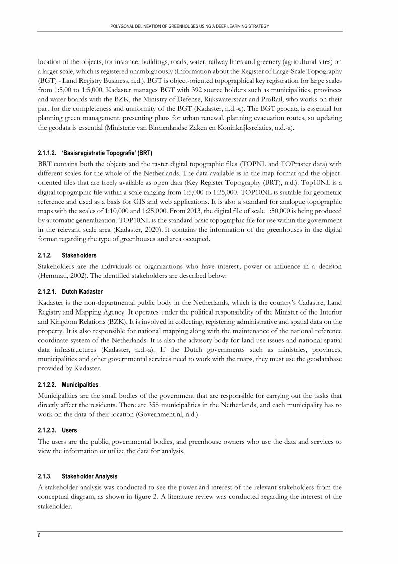
Table 2 summarises related studies on the instance segmentation with remote sensing datasets, methods
used, and the results, particularly for the buildings instances. There are no particular studies done on a
greenhouse on the relative method.
Table 2: Related studies on instance segmentation on buildings
Study
No
Title Remote
Sensing
Datasets
Method Results Reference
1 “Mask R-CNN” Natural images Mask R-CNN is
state of the art; in
instance
segmentation, a
branch for object
mask prediction in
parallel to the
existing branch of
bounding box
recognition is used.
In COCO suite
challenges, for
instance
segmentation,
person keypoint
detection and
bounding box
object detection, it
outperformed the
COCO 2016
winner.
(He et al.,
2020)
2 “Instance
Segmentation in
Remote Sensing
Imagery using
Deep
High resolution
orthogonal
aerial images
obtained from
earth explorer
Mask R-CNN is
used where
proposals are
generated in the
images classifies the
For the detection
of objects of
interest, the mean
average precision
(mAP) at the IoU
(Potlapally
et al.,
2019)
POLYGONAL DELINEATION OF GREENHOUSES USING A DEEP LEARNING STRATEGY
12
Study
No
Title Remote
Sensing
Datasets
Method Results Reference
Convolutional
Neural
Networks”
ROI for
segmentation mask
and bounding box
along with the
object of interest
such as tress, crop
fields, cultivated
lands and water
bodies.
threshold of 0.5
was 0.527.
3 “Automatic
Object
Extraction from
High-Resolution
Aerial Imagery
with Simple
Linear Iterative
Clustering and
Convolutional
Neural
Networks”
High-resolution
aerial images
The method uses
object extraction
similar to Fast R-
CNN architecture
and uses a simple
linear iterative
clustering (SLIC)
algorithm for ROI
generation.
Multi-scale SLIC
generates ROI of
different sizes and
objects detection
and segmentation
with an overall
accuracy (OA) of
89%.
(Carrilho
& Galo,
2019)
4 “Boundary
Regularized
Building
Footprint
Extraction from
Satellite Images
using Deep
Neural
Networks”
High-resolution
satellite images
of DigitalGlobe
Worldview-3
Satellite
The method,
namely R-
PolyGCN, is a two-
stage object
detection network
to produce ROI
features and use
graph models to
learn geometric
information for
building boundary
extraction.
The F1 score is
0.742 for building
extraction, and for
building
regularization, R-
PolyGCN predicts
the natural
representation for
the vertex, edges
and the polygon.
(K. Zhao
et al.,
2020)
5 “Object
Detection and
Instance
Segmentation in
Remote Sensing
Imagery Based
on Precise Mask
R-CNN”
VHR remote
sensing images
acquired from
Google Earth
The framework is
based on Mask R-
CNN, including
RPN and Fast R-
CNN classifier with
Precise RoI pooling
instead of RoI align.
For object
detection, AP is
61.2, and for
segmentation
performance, AP is
64.8.
(Su et al.,
2019)
6 “TernausNetV2:
Fully
convolutional
network, for
High-resolution
satellite imagery
FCN network called
TerausNetV2 uses
encoder-decoder
type architecture
with skip
For DeepGlobe-
CVPR 2018,
building detection
sub-challenge,
based on public
(Iglovikov
et al.,
2018)

POLYGONAL DELINEATION OF GREENHOUSES USING A DEEP LEARNING STRATEGY
13
Study
No
Title Remote
Sensing
Datasets
Method Results Reference
Instance
segmentation”
connection with the
encoder called ABN
WideResNet-38
network and in-
place activated
batch
normalization.
leaderboard score,
the model scored
0.74
7 “Building
Instance Change
Detection from
Large-Scale
Aerial Images
using
Convolutional
Neural Networks
and Simulated
Samples”
VHR aerial
images
The framework
consists of building
an extraction
network using Mask
R-CNN for object-
based instance
segmentation and
FCN for pixel-
based semantic
segmentation to
build a binary
building map.
Both object-based
and pixel-based
model’s evaluation
measured are used.
Without using a
real change sample,
the AP of building
instance was 0.63,
Precision of 0.64
and Recall of 0.943.
(Ji et al.,
2019)
8 “Topological
Map Extraction
from Overhead
Images”
VHR aerial
images
Method named
Polymapper for
pixel-wise
segmentation for
directly predicting
the polygons of the
buildings and the
roads. It uses CNN
as the backbone for
feature learning and
integrates with the
feature pyramid
network for
bounding boxes for
buildings. It uses a
skip feature map
with the bounding
box obtained and
RNN to get the
vertices of the
polygons of the
buildings.
Evaluated with the
standard MS
COCO measures
with AP of 55.7
and AR of 62.1. In
which AP and AR
for small buildings
were lower
compared to
medium and large
buildings.
(Z. Li et
al., 2019)
9 “Building Outline
Delineation:
From Very High-
Resolution
VHR aerial
images
Modified the
baseline method of
the PolyMapper by
using EffcientNet
For COCO metrics
on the building
delineation, the
applied method had
(W. Zhao
et al.,
2020)

POLYGONAL DELINEATION OF GREENHOUSES USING A DEEP LEARNING STRATEGY
14
Study
No
Title Remote
Sensing
Datasets
Method Results Reference
Remote Sensing
Imagery to
Polygons with an
Improved end-
to-end Learning
Framework”
as backbone feature
encoder to the
network and for
better prediction
accuracy of the
corner, using the
Boundary
Refinement block
(BRB).
an AP value of
0.445. The average
Recall value of
0.499. It can
correctly segment
the building
instances of various
shapes and sizes
with more compact
and regularized
shapes.
10 “Polygonal
Building
Segmentation by
Frame Field
Learning”
VHR aerial
images
Method named
Frame Field
Learning for pixel-
wise segmentation
and addition of
frame field as
output for
polygonization of
the buildings.
The method is
useful for the
regularization of
the sharp corners
of the building and
can handle holes in
the buildings and
walls in the
adjoining building.
(Girard et
al., 2020)
Table 3 describes the summary of related studies on the vectorization for deep building segmentation, which
is divided into two different categories with remote sensing datasets, methods used, description about the
method and the problems within the method for the buildings instances as there are no particular studies
done on a greenhouse on the comparative method.
Table 3: A related study on vectorization for deep building segmentation
S.No Category Method used Problems encountered
1. Classification
map produced
from deep
learning
network and
vectorizing the
classified map
Contour detection (marching
squares method (Lorensen & Cline,
1987)) for constructing 3D surfaces
by forming triangle modes of
constant density surfaces and
followed by polygon simplification
(Ramer, 1972) algorithm where
small-but not minimum-number of
vertices within the curve is utilized
to form a polygon.
Sharp corners are not produced when
the classification map is not perfect
when the conventional deep
segmentation method is used.
The expensive and complex post-
processing procedure required to
improve final polygons
In the classification map, the
approximate shape of the object is
done using the polygonal partition
refinement method(M. Li et al.,
2020), where progressively extended
detected line segments are added
together to form polygons. The
The tuneable parameter does not
control the exact number of output
vertices compared to the other
vectorization pipelines.

POLYGONAL DELINEATION OF GREENHOUSES USING A DEEP LEARNING STRATEGY
15
S.No Category Method used Problems encountered
trade-off between complexity and
fidelity is done using a tuneable
parameter.
FCN with a shared decoder and
discriminator was used to train with
the combination of adversarial and
regularized losses to produce
cleaner building footprints (Zorzi &
Fraundorfer, 2020).
The method is less stable than
conventional supervised learning as it
requires the computation of large
matrices of pairwise discontinuity
costs between pixels and the
adversarial training system of
networks.
2. Deep learning
segmentation
method to
directly learn
vector
representation
(end-to-end
method)
Curve-GCN method: The
prediction of all vertices
simultaneously using graph
convolutional network (GCN) is
trained to deform a polygon to fit
each object (Ling et al., 2019).
GCN is difficult to train compared to
CNN and is only suitable for simple
polygons without holes.
Polymapper method: It localizes the
object of interest with a
combination of the Feature
Pyramid Network (FPN) for
localization of the object of interest,
detection of Region of Interest
(ROI) in the image and
PolygonRNN for the geometrical
shape of the single (individual)
object (Z. Li et al., 2019).
It is not suitable for complex
buildings, and although adjacent
buildings are detected as individual
polygons, the shared edges within the
buildings are not aligned.

POLYGONAL DELINEATION OF GREENHOUSES USING A DEEP LEARNING STRATEGY
16
3. RESEARCH METHODOLOGY
The existing work for vectorization using deep building segmentation have two categories, i.e., an end-to-
end method that learns the vector representation directly, and the other is vectorizing the classification map
by a network. For delineation of greenhouses using deep learning methodology, both categories were
investigated in this study.
3.1. Method I: Polymapper
The polymapper method is the end-to-end learning method that directly extracts the object of interest's
polygon shape (mainly buildings and roads) with the provided aerial image and reference data. The method
is used to achieve instance segmentation of the geometrical shapes of the buildings in the aerial images.
Polymapper would help to detect (localize) all the objects of interest and precisely segment each object of
interest in the polygon representation rather than a per-pixel mask. Polymapper is the combination of the
Feature Pyramid Network (FPN) for localization of the object of interest, detection of Region of Interest
(ROI) in the image, and PolygonRNN for the geometrical shape of the single (individual) object (Z. Li et
al., 2019; W. Zhao et al., 2020).
Figure 4: Workflow of investigated polymapper method for buildings using RGB images and reference data
Adapted from : (Li, Wegner, & Lucchi, 2019)
3.2. Method II: Frame field learning
Girard, Smirnov, Solomon, and Tarabalka (2020) proposed a framework based on a deep image
segmentation model using remote sensing images for buildings. It utilizes FCN for pixel-wise classification
and adds frame fields to obtain buildings’ vectorized polygonization. Girard et al. (2020) has defined frame
field as a 4-PolyVector field which is locally defined by two symmetric line fields, called frames. The frame
is defined by two directions at each point in the image as two complex numbers 𝑢, 𝑣 ∈ C. The coefficients
are represented as the complex polynomial in which the two directions are converted into coded form with
relabelling and change of sign:
𝑓(𝑧) = (𝑧2 − 𝑢2)(𝑧2 − 𝑣2) = 𝑧4 + 𝑐2𝑧2 + 𝑐0 (1)
Within the set of pairs of directions, the constants 𝑐0 , 𝑐2 ∈ 𝐶 uniquely determines an equivalence class
corresponding to a frame. The equation (1) can be denoted as 𝑓(𝑧; 𝑐0 , 𝑐2). One of the pair of directions,
(𝑐0 , 𝑐2) pair can be recovered by defining the corresponding frame:

POLYGONAL DELINEATION OF GREENHOUSES USING A DEEP LEARNING STRATEGY
17
{ 𝑐0 = 𝑢
2𝑣2
𝑐2 = −(𝑢2 + 𝑣2)
⟺
{
𝑢2 = −
1
2 (𝑐2 + √𝑐2
2 − 4𝑐0)
𝑣2 = −1
2 (𝑐2 −√𝑐2
2 − 4𝑐0)
(2)
With equation (1), a smooth frame field with the property along building edges is learned such that at least
one field direction is aligned to the polygon tangent direction. Girard et al. (2021) used PolyVector fields
rather than vector fields to align the field to the tangent direction at the polygon corners. The frame field is
used to prevent the corners of the polygon from being cut off. The neural network learns the field at every
pixel of the image. The learning of (𝑢, 𝑣) pair per pixel is challenging due to labelling and sign so, the
constant (𝑐0 , 𝑐2) pair is learnt in this method which has no sign or ordering ambiguity.
The original frame field learning method takes H x W RGB image I as input, and the output is a classification
map and a frame field. The classification map is made up of two channels, i.e., building interiors (𝑦𝑖𝑛𝑡) and
the building boundaries (𝑦𝑒𝑑𝑔𝑒). The frame field consists of four channels corresponding to the two
coefficients 𝑐0 , 𝑐2 ∈ 𝐶. The original method utilizes a deep segmentation model as a backbone. This thesis
uses U-net Resnet101 architecture as the backbone with a two-channel output corresponding to object
interiors and contours. The training is supervised, which requires input image with labelled ground truth
�̂�𝑖𝑛𝑡. The edges mask, and interior masks are generated from the polygons on the reference dataset by
rasterizing them, which is the pre-processing part of the algorithm. The angle calculated from the segments
of the reference data is used for the frame field. The model learns the feature extraction from the input data
and, with the help of combined loss functions, constrain these tasks to make them consistent.
The segmentation is improved via multi-task learning with the addition of frame fields aligned to object
tangents. The method trains the network for pixel-wise classification of objects followed by additional
learning of frame field aligned for the object outlines. The method introduces a frame field that increases
segmentation performances, such as yielding sharper corners and vectorization information (Girard et al.,
2021). Frame field is added to leverage the polygonization with additional structural information and allow
complexity tuning of the corner-aware simplification step for handling non-trivial building topology.
Figure 5: Workflow of investigated frame field learning method for building and adapted for greenhouse delineation by fusing RGB,
nDSM data and reference data
Adapted from : (Girard, Smirnov, Solomon, & Tarabalka, 2020)

POLYGONAL DELINEATION OF GREENHOUSES USING A DEEP LEARNING STRATEGY
18
The input images with the reference data are utilized for segmentation. The base line method frame field
learning only utilizes the RGB band, but in this study, nDSM is added to the first layer of the network as
the additional layer so that the input images will have four channels. The output features of the backbone
are fed to the shallow structures so that the frame field (utilizing four channels) and segmentation (utilizing
two channels of the image) are produced.
3.2.1. Loss Function
During the training, there are three different tasks where loss functions were prevalent: a) segmentation, b)
frame field and c) coupling losses. The height and width of the input image are denoted by H and W, where
linear combined segmentation loss for cross-entropy function and dice function of the edge mask and the
interior mask is defined by:
𝐿𝐵𝐶𝐸 (�̂�, 𝑦) = 1
𝐻𝑊 ∑ �̂�(𝑥). log(𝑦(𝑥)) + (1 − �̂�(𝑥)). log(1 − 𝑦(𝑥)) ,
𝑥 ∈ 𝐼
(3)
𝐿𝐷𝑖𝑐𝑒 (�̂�, 𝑦) = 1 − 2 . |�̂� . 𝑦| + 1
|�̂� + 𝑦| + 1, (4)
𝐿𝑖𝑛𝑡 = 𝛼 . 𝐿𝐵𝐶𝐸 (�̂�𝑖𝑛𝑡 , 𝑦𝑖𝑛𝑡) + (1 − 𝛼) . 𝐿𝐷𝑖𝑐𝑒 (�̂�𝑖𝑛𝑡 , 𝑦𝑖𝑛𝑡), (5)
𝐿𝑒𝑑𝑔𝑒 = 𝛼 . 𝐿𝐵𝐶𝐸 (�̂�𝑒𝑑𝑔𝑒 , 𝑦𝑒𝑑𝑔𝑒) + (1 − 𝛼) . 𝐿𝐷𝑖𝑐𝑒 (�̂�𝑒𝑑𝑔𝑒 , 𝑦𝑒𝑑𝑔𝑒), (6)
where, 𝐿𝐵𝐶𝐸 is the binary cross-entropy loss applied and 𝐿𝐷𝑖𝑐𝑒 is the dice loss for the interior mask and the
edge mask output of the model. Furthermore, the 𝛼 is the hyperparameter with the value ranging from 0
and 1.
Figure 6: Two branches to produce segmentation and frame field
The frame field is another output from the network obtained through the addition of a fully convolutional
network via a module consisting of a sequence of 2 x 2 convolution, batch normalization, an exponential
linear unit (ELU) nonlinearity, another 2 x 2 convolution and tanh nonlinearity. The concatenation of the
segmentation output and the output feature of the backbone network layer from the frame field. The ground
truth label is the angle 𝜃𝜏 ∈ [0, 𝜋) of the unsigned tangent vector of the polygon contour. Three losses are
considered to train the frame field, which is given by
𝐿𝑎𝑙𝑖𝑔𝑛 = 1
𝐻𝑊 ∑�̂�𝑒𝑑𝑔𝑒(𝑥)𝑓(𝑒
𝑖𝜃𝜏 ; 𝑐0(𝑥), 𝑐2(𝑥))2
𝑥∈𝐼
, (7)

POLYGONAL DELINEATION OF GREENHOUSES USING A DEEP LEARNING STRATEGY
19
𝐿𝑎𝑙𝑖𝑔𝑛90 = 1
𝐻𝑊 ∑�̂�𝑒𝑑𝑔𝑒(𝑥)𝑓(𝑒
𝑖𝜃𝜏⟂ ; 𝑐0(𝑥), 𝑐2(𝑥))2
𝑥∈𝐼
, (8)
𝐿𝑠𝑚𝑜𝑜𝑡ℎ = 1
𝐻𝑊 ∑(||∇𝑐0(𝑥)||
2+ ||∇𝑐2(𝑥)||
2)
𝑥∈𝐼
, (9)
The 𝜃𝜔 is the direction of vector 𝜔 = ||𝜔||2𝑒𝑖𝜃𝜔 and 𝜏⟂ = 𝜏 −
𝜋
2. The losses of the different properties
of the output field, which is described by 𝐿𝑎𝑙𝑖𝑔𝑛 makes the frame field aligned with the tangent direction of
the line segment of the polygon, 𝐿𝑎𝑙𝑖𝑔𝑛90 events the frame field from collapsing into the line field and
𝐿𝑠𝑚𝑜𝑜𝑡ℎ is the Dirichlet energy, which measures the smoothness of the function within the location of x in
the image.
With different outputs such as interior and boundary segmentation masks, the frame field must be
compatible with one another, so coupling losses are added for mutual consistency.
𝐿𝑖𝑛𝑡 𝑎𝑙𝑖𝑔𝑛 = 1
𝐻𝑊 ∑ 𝑓(∇𝑦𝑖𝑛𝑡(𝑥); 𝑐0(𝑥), 𝑐2(𝑥))
2
𝑥 ∈ 𝐼
, (10)
𝐿𝑒𝑑𝑔𝑒 𝑎𝑙𝑖𝑔𝑛 = 1
𝐻𝑊 ∑ 𝑓 (∇𝑦𝑒𝑑𝑔𝑒(𝑥); 𝑐0(𝑥), 𝑐2(𝑥))
2
𝑥 ∈ 𝐼
, (11)
𝐿𝑖𝑛𝑡 𝑒𝑑𝑔𝑒 = 1
𝐻𝑊 ∑ max(1 − 𝑦𝑖𝑛𝑡(𝑥),
𝑥 ∈ 𝐼
ǁ∇𝑦𝑖𝑛𝑡(𝑥)ǁ 2). |ǁ∇𝑦𝑖𝑛𝑡(𝑥)ǁ 2 − 𝑦𝑒𝑑𝑔𝑒 (𝑥)|
(12)
where, 𝐿𝑖𝑛𝑡 𝑒𝑑𝑔𝑒 aligns the spatial gradient of the predicted interior map 𝑦𝑖𝑛𝑡 with the frame field.
𝐿𝑒𝑑𝑔𝑒 𝑎𝑙𝑖𝑔𝑛 aligns the spatial gradient of the predicted edge map 𝑦𝑒𝑑𝑔𝑒 with the frame field. 𝐿𝑖𝑛𝑡 𝑒𝑑𝑔𝑒 aligns
the interior mask and edge compatible with each other. The eight losses have different scales and are linearly combined using eight coefficients, so the normalization
coefficient 𝑁(𝑙𝑜𝑠𝑠 𝑛𝑎𝑚𝑒) by averaging each loss on a random subset of the training dataset using a randomly
initialized network. The normalization aims to rescale each loss equally, and the combination of main losses
and regularization losses are made with parameter 𝜆 ∈ [0,1]:
𝜆 (𝐿𝑖𝑛𝑡 𝑁𝑖𝑛𝑡
+ 𝐿𝑒𝑑𝑔𝑒
𝑁𝑒𝑑𝑔𝑒+ 𝐿𝑎𝑙𝑖𝑔𝑛
𝑁𝑎𝑙𝑖𝑔𝑛) + (1 − 𝜆)(
𝐿𝑎𝑙𝑖𝑔𝑛90
𝑁𝑎𝑙𝑖𝑔𝑛90+ 𝐿𝑠𝑚𝑜𝑜𝑡ℎ 𝑁𝑠𝑚𝑜𝑜𝑡ℎ
+ 𝐿𝑖𝑛𝑡 𝑎𝑙𝑖𝑔𝑛
𝑁𝑖𝑛𝑡 𝑎𝑙𝑖𝑔𝑛+ 𝐿𝑒𝑑𝑔𝑒 𝑎𝑙𝑖𝑔𝑛
𝑁𝑒𝑑𝑔𝑒 𝑎𝑙𝑖𝑔𝑛 +
𝐿𝑖𝑛𝑡 𝑒𝑑𝑔𝑒
𝑁𝑖𝑛𝑡 𝑒𝑑𝑔𝑒) (13)
In the original framework, the bias was set with the value 𝜆 = 0.75, and in this thesis, it is also set to 0.50.
3.2.2. Polygonization
For polygonization, interior mask and frame field are the input where the initial contour is extracted from
the interior map using the marching squares method (Lorensen & Cline, 1987). Then they are optimized
with the active contour method (ACM), which is made to align to the frame field. The corner-aware polygon
POLYGONAL DELINEATION OF GREENHOUSES USING A DEEP LEARNING STRATEGY
20
simplification was utilized by detecting the building corner vertices, one of the important vertices required
for delineation.
The polyline collection is polygonised with a list of polygons to detect the building polygons in a planar
graph with the building probability value for each polygon with the predicted interior probability map and
removing the low-probability polygons.
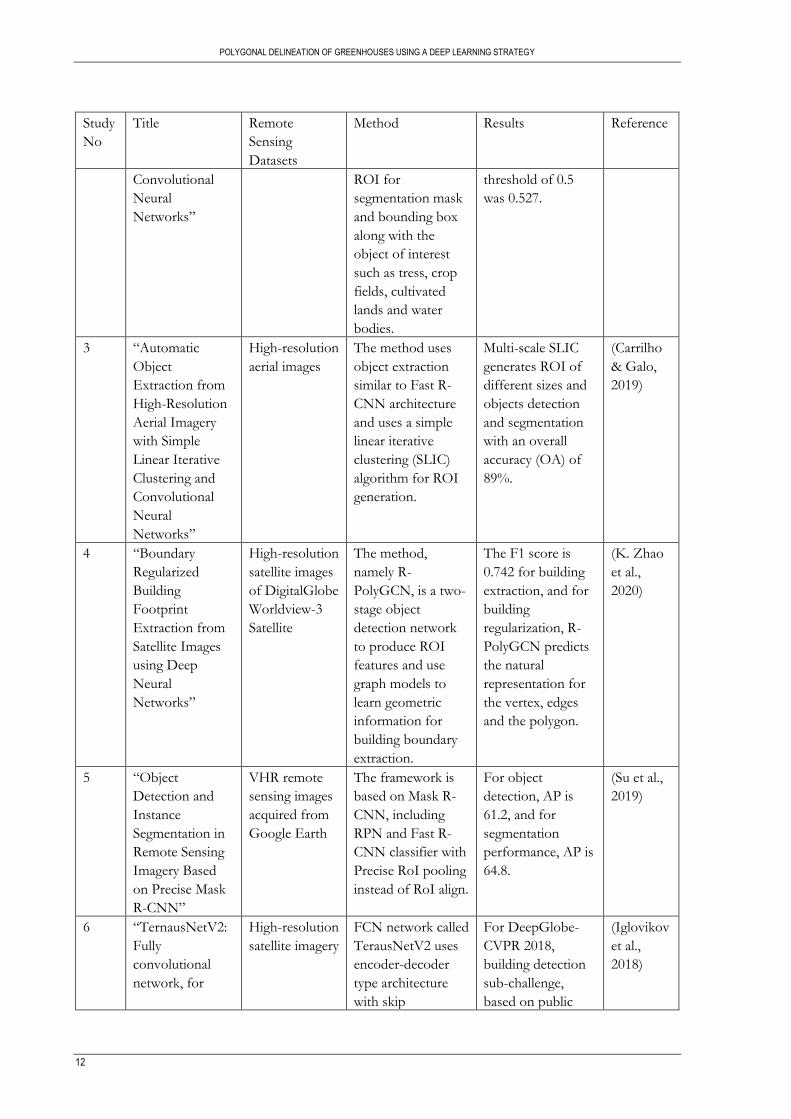
Figure 7: ArcGIS model for aggregating different individual greenhouses separated in the largely dispersed geographical area as shown in
figure 9
The output of the predicted test tiles had individual shapefiles per tile. As per the BRT dataset, the size of
the greenhouse ranges from 200 sqm to 589653.408 sqm. Since the size of the greenhouses are big and
distributed over a large geographical area, a model in ArcGIS was created to aggregate the predicted
individual greenhouses in the test dataset. The greenhouses which were separated into two or more tiles,
would delineate separately as the model outputs the polygonization per image tiles in the test dataset. For
joining such greenhouses together, the ArcGIS model was implemented. The individual predicted shapefiles
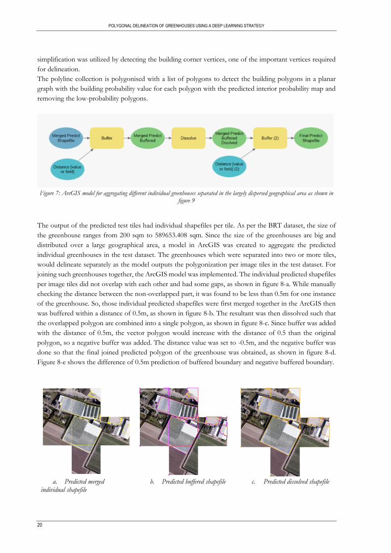
per image tiles did not overlap with each other and had some gaps, as shown in figure 8-a. While manually
checking the distance between the non-overlapped part, it was found to be less than 0.5m for one instance
of the greenhouse. So, those individual predicted shapefiles were first merged together in the ArcGIS then
was buffered within a distance of 0.5m, as shown in figure 8-b. The resultant was then dissolved such that
the overlapped polygon are combined into a single polygon, as shown in figure 8-c. Since buffer was added
with the distance of 0.5m, the vector polygon would increase with the distance of 0.5 than the original
polygon, so a negative buffer was added. The distance value was set to -0.5m, and the negative buffer was
done so that the final joined predicted polygon of the greenhouse was obtained, as shown in figure 8-d.
Figure 8-e shows the difference of 0.5m prediction of buffered boundary and negative buffered boundary.
a. Predicted merged individual shapefile
b. Predicted buffered shapefile
c. Predicted dissolved shapefile

POLYGONAL DELINEATION OF GREENHOUSES USING A DEEP LEARNING STRATEGY
21
d. Predicted final shapefile
e. Zoomed layer showing the buffered and negative buffered result
Figure 8: Application example of ArcGIS model on the test dataset

POLYGONAL DELINEATION OF GREENHOUSES USING A DEEP LEARNING STRATEGY
22
4. MATERIALS
This chapter introduces the study area where the research was conducted, followed by the datasets used.
Finally, the description of the data preparation is described.
4.1. Study Area
This research was applied to three different provinces of the Netherlands out of twelve, namely Noord-
Holland, Zuid-Holland and Noord-Brabant. Based on the BRT dataset for the greenhouses in the year 2019,
there were 13306 greenhouses covering an area of 132829632.50 sq m (132.83 sq km) in the Netherlands.
Out of which, 2131 greenhouses covering an area of 1333163.85 sq m (1.33 sq km) were distributed in these
three provinces. There were mainly two types of greenhouses present in the area, made up of glasses and
plastic. The commercialized greenhouses and movable greenhouses were mainly made up of glasses while,
in the farm area (rural part), a few plastic greenhouses were present. Greenhouses had been used for different
purposes, such as department stores and greenhouse warehouses for horticulture and vegetation.
Greenhouses in the Netherlands are distributed throughout the country, but the study area was selected
such that commercialized greenhouses, movable greenhouses, small greenhouses were present. Also,
greenhouses near building areas were considered.
Figure 9: Location of the study area with the distribution of training, testing and validation tiles
4.2. Data
The dataset contains three parts: a) A VHR orthophoto aerial image, b) nDSM generated from stereo
imagery, and c) BRT polygon of the greenhouse as reference data.
4.2.1. Aerial Imagery
A nationwide aerial photo of the Netherlands is captured bi-annually during the summer and winter months
in different resolutions. The dataset with 0.25 m resolution is freely available to the public. Another dataset
is of 0.1 m resolution, used internally. The raw aerial imagery is collected and processed to prepare
orthophotos geometrically corrected with uniform scale in the “RD-New” map projection as accepted in
the Netherlands. After quality control, the final product is made available to the general public (Kadaster,
n.d.-b). Two different orthoimages were utilized for the experimental analysis in this study, which is
described below:

POLYGONAL DELINEATION OF GREENHOUSES USING A DEEP LEARNING STRATEGY
23
4.2.1.1. Winter dataset (0.1m resolution dataset)
The winter dataset is the aerial imagery (orthophotos) with the spatial resolution of 10 cm, which is an
internal dataset from Kadaster. The aerial dataset utilized was from 2019 for all the training, validation and
testing tiles. The orthophotos were of the size 1024x1024 with the file extension of .png as provided by
Kadaster. The .png image file also contains a .wld formatted ESRI World (WLD) file containing control
points that describe coordinate information for a raster image, including its pixel size, rotation, and
coordinate location (ESRI, 2016).
4.2.1.2. Summer dataset (0.25m resolution dataset)
The summer data is freely available to the users via the Publieke Dienstverlening Op de Kaart (PDOK),
which translates to Public Services On the Map website. It contains up-to-date and reliable geo datasets. It
contains orthophoto mosaics of the entire country with RGB and Color Infrared (CIR) bands. The CIR
band was removed, and only the RGB band was used for experimental analysis. A maximum of 5 years of
orthophoto mosaics are available meaning, 2015 – 2019 is available (PDOK, n.d.-a). The summer dataset is
the freely available imagery dataset with a resolution of 0.25m from the year 2019.
a. Orthophoto (Aerial Image) b. Normalized Digital Surface Model (nDSM)
c. BRT dataset as the reference data overlapping the aerial image
Figure 10: List of data used
4.2.2. Normalized Digital Surface Model (nDSM)
The nDSM used was also confidential data from Kadaster, which was derived from the VHR stereo imagery.
With the overlapped stereo images, the feature points were determined and matched from which 3D
coordinates were extracted from the points, which gave the information of 3D information. The nDSM
provided was in the form of a raster image with the extension .tif. The nDSM provided the height
information of what lies above the ground with a resolution of 0.20m. For winter images, nDSM was
resampled into 0.1m.
4.2.3. Greenhouse footprints
The polygonal data was in the ESRI geodatabase format, which can be downloaded from pdok.nl. The
greenhouse was one of the attributes within the ‘Buildings’ category on the TOP10NL product of BRT.
Two different categories of the greenhouse were considered “overig|kas,warenhuis” and “kas, wareinhuis”,
which translated to “other|greenhouse department store” and “greenhouse, warehouse”, respectively.
There was no separation of plastic greenhouses or glass greenhouses within the attribute of the dataset. The
BRT polygons are updated yearly, and the greenhouse footprints of the year 2019 were used for reference
purposes.

POLYGONAL DELINEATION OF GREENHOUSES USING A DEEP LEARNING STRATEGY
24
4.3. Data Preprocessing
The data used in this thesis was VHR resolution images, limiting the research area’s size under a certain
number of pixels. This is the reason why within the three provinces, not all the greenhouses in the three
provinces were selected.
4.3.1. Tiles Preparation, selection and distribution
The training, testing, and validation tiles were distributed over the study area such that geographical
knowledge is considered, as mention in section 4.1. Stratified sampling techniques were used within the
dataset for training, testing and validation such that there is less class imbalance in terms of greenhouse class
and non-greenhouse class. The whole dataset was divided into a sample of a homogeneous dataset with
specific criteria. The tiles were distributed for training, validation and testing in which 50% of the tiles were
randomly selected, while 50% of the tiles were manually selected. The criteria for selecting the tiles were to
have both the glasses greenhouses and the plastic greenhouses. Also, while randomly selecting the tiles, a
complete boundary of the greenhouse was not selected due to big sized greenhouses. It means that a part
of the greenhouse was being separated as different sets of grouped tiles (validation, training and testing).
So, the tiles were manually selected such that a complete polygon lies within a set of grouped tiles. The
separation of training, testing and validation tiles were considered with the changes in the greenhouse. The
tiles of 1024x1024 were generated using the “Create Fishnet” tools in the ArcGIS for the 0.1m dataset. The
tiles were used to clip the images as well as the nDSM.
a. Winter dataset (0.1m resolution)
For 0.1m resolution data, the raster information on the number of columns and the rows was made sure
that the rows were 1024x1024 with the cell size to be 0.1. The nDSM was also resampled to 0.1m which
was stacked as a 4th channel on top of the RGB images to produce a composite image.
b. Summer dataset (0.25m resolution)
For summer images with the resolution of 0.25m, the tiles generated from the same procedure was of
512x512 such that the cell size was set to 0.25 and the number of columns and rows set to 512x512. The
tiles area was considered such that it includes the same area for training, testing and validating areas as
compared to the winter dataset. The summer images had some changes in the greenhouses area. Since the
time to capture the images was different from the winter dataset, new greenhouses were being built, some
greenhouses were being extended, and some greenhouses were demolished.
From the total tiles, 60% of the tiles were selected as training tiles, 20% of tiles as validation and 20% of the
tiles as testing datasets. Due to tiles with incomplete polygon among the tiles, the distribution of the tiles
was not exactly within the ratio of 60:20:20 for training, testing and validation. The tile distribution, tile size
and number of greenhouses within the tiles are shown in the table 4.

POLYGONAL DELINEATION OF GREENHOUSES USING A DEEP LEARNING STRATEGY
25
Table 4: Information on the tiles used for different datasets, training, validation, and test dataset for experimental analysis
Dataset Tiles size Type Number of Tiles Number of
greenhouses
RGB and
RGB+nDSM
(0.1m)
1024x1024 training 2303 1760
validation 422 147
test 512 224
RGB and RGB
(0.25m)
512x512 training 1816 1748
validation 302 147
test 398 224
4.3.2. Annotation of the reference dataset
Every individual image tile had its own reference dataset. The name of the tiles of images and the reference
data were the same. The reference data, i.e., the polygon of the greenhouse from BRT, was first clipped with
respect to the image tiles using the “Clip” tool in ArcGIS. The clipped greenhouse was then split into
individual shapefiles using the ArcGIS tool “Split by Attributes”. It was used such that the split shapefile
would have the same name as the image, with the split field being the name of the image. Two different
annotation format was utilized in the thesis which are described below:
a. COCO format
COCO (Common Objects in COntext) format is used mainly in object recognition and scene understanding.
The coco format is considered the de facto standard to store the annotations of the object of interest
(Waspinator, 2018). It uses .json (JavaScript Object Notation) to encode information about a dataset. It
includes the “info”, “licenses”, “categories”, and “images” lists which represents the shapefiles metadata
which is written as per the user. The annotations attributes contain information about the bounding box,
area, segmentation (shape of the greenhouse), image_id, height and width of the tiles. Figure 11 shows the
example of the annotation format for one of the shapefiles and its corresponding image saved in the coco
format (Waspinator, 2018).
Figure 11: One of the BRT polygons in COCO dataset JSON format

POLYGONAL DELINEATION OF GREENHOUSES USING A DEEP LEARNING STRATEGY
26
b. GeoJSON format
The geographic features with the information of the nonspatial format are represented in an open standard
geospatial data interchange format termed GeoJSON format (ESRI, n.d.). It is based on the JavaScript
Object Notation(JSON) format with information on the type, geographic coordinate reference system,
geometry types, and shapefile properties. A snippet of one of the shapefile in the geoJSON file format is
shown in figure 12.
Figure 12: BRT polygon dataset in geoJSON format
4.3.3. Dataset Preparation for the Polymapper
The dataset for the greenhouse was prepared using the aerial image of 0.1m resolution and reference data
shapefile of greenhouses from the BRT, shown in figure 13. The shapefile of the reference data was
transformed into COCO format to use the method of polymapper, which is shown in figure 10.
a) 0.1m ortho-image b) BRT reference data polygon c) Individual polygon per tiles
Figure 13: Aerial imagery and reference data (BRT polygon) preprocessing
The shapefiles were generated such that the polygon of the object of interest (in this case: greenhouse) was
made within the image tiles, meaning that training, validating and testing image tiles and shapefiles with
respect to each image tile were equal.
4.3.4. Training the model and reasons for not using Polymapper method for greenhouse
The model was trained with the datasets prepared for the greenhouses. While evaluating the trained model
on the test dataset, it did not work. The reason was that the method needs to have at least one complete
object of interest per image, i.e., the object of interest (at least one closed polygon per image). Since the
greenhouses in the Netherlands are bigger in size with the area of greenhouses which has area up to 500000
sqm., so the initial tiles of 1024 x 1024 was not suitable as a tile did not contain the complete polygon of the
greenhouse, but it was divided into different other tiles. The option for bigger image tiles was also not
possible because of the cloud machine’s memory issues and computational efficiency.

POLYGONAL DELINEATION OF GREENHOUSES USING A DEEP LEARNING STRATEGY
27
4.3.5. Data Preparation for Frame Field Learning
The dataset tiles were prepared same as mentioned in the section 4.3.1. The dataset for the greenhouse was
prepared using the aerial image of 0.1m resolution for winter images, 0.25m resolution for summer image
and reference data shapefile of greenhouses from the BRT, shown in figure 13. The shapefile of the
reference data per individual tiles was transformed into geoJSON format to use the method of frame field
learning method. Furthermore, the mean and the standard deviation of all the training images, testing images
and validation images were calculated as it is one of the inputs that need to be set in the model. To train the
frame field learning model applicable for greenhouses, two different resolutions of images were taken into
account with configuration described in the section 5.1.

POLYGONAL DELINEATION OF GREENHOUSES USING A DEEP LEARNING STRATEGY
28
5. EXPERIMENTAL ANALYSIS
This chapter describes the experimental analysis done with the information on the configuration,
combination of the dataset used, and the evaluation metrics used in the research.
5.1. Configuration
The model was trained with the following settings:
Optimizer: Adam
Batch size: 1
(Due to CUDA memory error, batch size could
not be increased for 0.1m dataset)
Initial learning rate: 0.00001
Exponential decay rate for the learning rate: 0.9
Maximum epoch: 50
Binary cross-entropy: 0.25 (first configuration) and 0.5 (second
configuration)
Dice Coefficient: 0.75 (first configuration) and 0.5 (second
configuration)
Polygonization parameter:
Tolerance: (0.125, 1, 9)
The network is implemented in PyTorch 1.4 and run in a single NVIDIA Tesla P10 GPU setting.
5.2. Combination of the dataset for experimental analysis
Table 5 shows the combination of the datasets for experiment analysis with reference dataset used. Table 5: Information on the datasets used for the experimental analysis
Experiment
Analysis
Orthoimage of
Resolution
Bands Reference
Dataset
Parameter Tuning
0.1m (winter data) RGB Original Shapefile
of BRT
RGB Edited (digitized
BRT) shapefile
BCE and Dice
coefficient change,
tolerance for
polygonization
RGB + nDSM Edited (digitized
BRT) shapefile
BCE and Dice
coefficient change,
tolerance for
polygonization
0.25m (summer
data)
RGB Edited (digitized
BRT) shapefile
BCE and Dice
coefficient to be of
value 0.25 and 0.75
respectively

POLYGONAL DELINEATION OF GREENHOUSES USING A DEEP LEARNING STRATEGY
29
5.3. Evaluation Metrics
The quantitative and qualitative result on the experimental analysis in section 5.2. is done based on the combination of the metrics:
5.3.1. Quantitative Analysis
The section describes the metrics that was used during the study.
a) Pixel-level metrics
It represents the per cent of the pixels in the predicted result on the image classified correctly with the
reference dataset. In the thesis, Intersection-Over-Union(IoU) is used, which is computed by dividing the
area of overlap or intersected area by the area of the union between the predicted segmentation area (𝑝)
and the ground truth (𝑔) (Tiu, 2019).
𝐼𝑜𝑈 =𝑎𝑟𝑒𝑎 (𝑝 ∩ 𝑔)
𝑎𝑟𝑒𝑎 (𝑝 ∪ 𝑔)
b) Object-level metrics
The delineation of the object of interest is the greenhouse in the thesis, which can be related to object
segmentation. For this purpose, mean Average Precision (AP) and mean Average Recall (AR) was calculated
with the evaluation metrics used by Common Objects in Context (COCO). The AP and AR have averaged
over 10 IoU threshold values of 0.50:0.05:0.95 with 0.05 steps. For better localization, averaging over IoU
is calculated (COCO - Common Objects in Context, n.d.). AP represents the correctly predicted positive
observation ratio to the total predicted positive observation within the IoU threshold. AR represents the
ratio of the correctly predicted positive observation to all the predicted observations as the positive class.
As per the standard COCO evaluation performance for the object detection, the following metrics are
calculated:
Average Precision (AP)
AP AP at IoU=0.50:0.05:0.95
APIoU=.50 AP at IoU=0.50
APIoU=.75 AP at IoU=0.75
AP Across Scales
APsmall AP for small objects: area < 322
APmedium AP for medium objects: 322 < area < 962
APlarge AP for large objects: area > 962
Average Recall (AR)
ARmax=1 AR given 1 detection per image
ARmax=10 AR given 10 detection per image
ARmax=100 AR given 100 detection per image
AR Across Scales
ARsmall AR for small objects: area < 322
ARmedium AR for medium objects: 322 < area < 962
ARlarge AR for large objects: area > 962
The standard metrics have evaluation metrics with small objects with an area less than 322 pixels, medium
objects with an area between 322 and 962 pixels and large objects with an area greater than 962 pixels. AP
and AR with the scales of the area are calculated where an area is measured as the number of pixels in the
segmentation mask. It was calculated using the standard COCO evaluation for detection metrics by
comparing the predicted dataset with the reference dataset.

POLYGONAL DELINEATION OF GREENHOUSES USING A DEEP LEARNING STRATEGY
30
5.3.2. Qualitative Analysis
Visual inspection or human interpretation was used to check the delineated greenhouse to see if the
greenhouse delineations were smooth and free of noise. The test tiles were visually inspected to see whether
the predicted boundary of the greenhouse was delineated correctly or not. It was also used to see the false
positives of the predicted greenhouses and to see where false positives were common compared to other
non-greenhouses classes.

POLYGONAL DELINEATION OF GREENHOUSES USING A DEEP LEARNING STRATEGY
31
6. RESULT AND DISCUSSION
This chapter includes the quantitative and qualitative analysis of the result obtained from the study. The
results are discussed and are followed by the limitation of the research.
The results on the test dataset of the aerial images (RGB) and composite images (RGB+nDSM) within the
study area were compared. The model configurations were kept the same to ensure a fair comparison of the
experimental analysis while changing the input dataset.
6.1. Quantitative analysis
Table 6 and 7 shows the quantitative results of different experimental analyses done on a different dataset
combination as described in section 5.2.
6.1.1. Training on the hyperparameter BCE of 0.25 and Dice Coefficient of 0.75
Table 6: Extracted result on the test dataset on the entire study area with the calculation of mean IoU and standard AP and AR (COCO metrics) for hyperparameter BCE of 0.25 and Dice coefficient of 0.75
Metrics RGB (0.1m) RGB+nDSM
(0.1m)
RBG (0.25m)
Mean IoU 0.673 0.751 0.745
AP IoU=0.50:0.05:0.95 0.005 0.003 0.003
APIoU=.50 0.010 0.007 0.011
APIoU=.75 0.006 0.004 0.006
APsmall 0.000 0.000 0.000
APmedium 0.011 0.008 0.010
APlarge 0.019 0.017 0.020
ARmax=1 0.037 0.037 0.038
ARmax=10 0.056 0.058 0.054
ARmax=100 0.058 0.058 0.054
ARsmall 0.000 0.000 0.000
ARmedium 0.024 0.017 0.022
ARlarge 0.063 0.064 0.063
Here, the value of APlarge and ARsmall was 0, which showed that the small greenhouse under the 322 pixels
and for 0.1 sqm resolution was not visible because the greenhouse was not as small as the greenhouse area
bigger than 322 x 0.12 pixel value. With the threshold of IoU = 0.50, AP of 0.1m RGB images was higher
than the RGB + nDSM images indicating that there was the low false positive rate for RGB images, while
0.25 m RGB has the highest among three which indicates that among the three band combination, 0.25 m
RGB had low false positive rate. Whereas, RGB + nDSM for 0.1m images had high mean AR value
indicating that there were few false negatives. The AP IoU=0.50:0.05:0.95 value for 0.1m RGB images was greater
than the AP IoU=0.50:0.05:0.95 for 0.1m RGB + nDSM with the value of 0.003, meaning within the threshold
from 0.5 to 0.95 with the steps of 0.05, the localization was better for 0.10m RGB images.
6.1.2. Training on the hyperparameter BCE of 0.50 and Dice Coefficient of 0.50
Table 7: Extracted result on the test dataset on the entire study area with the calculation of mean IoU and standard AP and AR (COCO metrics) for hyperparameter BCE of 0.50 and Dice coefficient of 0.50

POLYGONAL DELINEATION OF GREENHOUSES USING A DEEP LEARNING STRATEGY
32
Metrics RGB (0.1m) RGB+nDSM
(0.1m)
Mean IoU 0.784 0.807
AP IoU=0.50:0.05:0.95 0.006 0.004
APIoU=.50 0.011 0.008
APIoU=.75 0.007 0.004
APsmall 0.000 0.000
APmedium 0.009 0.009
APlarge 0.011 0.015
ARmax=1 0.049 0.040
ARmax=10 0.052 0.047
ARmax=100 0.052 0.047
ARsmall 0.000 0.000
ARmedium 0.020 0.020
ARlarge 0.058 0.052
With the hyperparameter changed from 0.25 to 0.50 for BCE and 0.75 to 0.75 for Dice coefficient, the mean
IoU has increased from 0.673 to 0.784 for 0.10m RGB images and from 0.751 to 0.807 for 0.10m RGB +
nDSM images. The AP IoU=0.50:0.05:0.95 value for 0.1m RGB images with the value of 0.006 was greater than
the AP IoU=0.50:0.05:0.95 for 0.1m RGB + nDSM value of 0.004, meaning within the threshold from 0.5 to 0.95
with the steps of 0.05, the localization was better for 0.10m RGB images. With the change of
hyperparameter, the accuracy had increased and can be seen in table 7 compared to table 6.
6.2. Qualitative Analysis
The prediction on 0.1m RGB bands after the training the model resulted in following
Reference Dataset Prediction on 0.1m RGB dataset using original BRT shapefile Figure 14: Prediction on 0.1m RGB dataset using original BRT shapefile done on frame field learning method
Initially, an experiment was conducted with the original datasets from BRT with the frame field learning
method. As the area for tiles preparation was selected such that there were changes in terms of greenhouses
along with different bigger and smaller greenhouses, the prediction of greenhouses were not good. The
greenhouses were being predicted not only in the area where there were greenhouses but also in the

POLYGONAL DELINEATION OF GREENHOUSES USING A DEEP LEARNING STRATEGY
33
vegetation, roads, bare soil areas, and some in the buildings. The reference dataset from BRT was rechecked
again and found that there were greenhouses where the image and the reference data polygon were not
overlapping with each other, which is seen in figure 15-a. Within the datasets that were prepared for training
the datasets initially, it was found that some of the greenhouses were not digitized so the model might have
learnt the textural feature and the spectral information of the other classes rather than the greenhouses.
a. Reference data of the greenhouse not overlapping the image.
b. A shift of the greenhouse
Figure 15: Errors in BRT shapefile within the dataset created
Some of the reference data of the greenhouse were incomplete, meaning only a certain part of the
greenhouse had overlapped boundary, while the rest of the greenhouse in the image was not overlapped.
Also, some greenhouses have been changed from greenhouse to house and are not updated, resulting in the
reference data being something else (e.g. houses) instead of the greenhouse.
Missing greenhouse reference data
Missing shapefile in the greenhouse (BRT shapefile not properly updated)
Mistake in reference data dataset of greenhouse
Figure 16: Missing BRT polygons and few errors on the BRT polygon shapefile

POLYGONAL DELINEATION OF GREENHOUSES USING A DEEP LEARNING STRATEGY
34
The dataset was corrected by manually digitizing the polygons which did not match with the orthoimage of
2019. The BRT shapefile where greenhouses were missing, non-overlapped greenhouses, shifted
greenhouses were digitized.
The qualitative result obtained in the test set of the aerial images with the dataset combination in section 5.2
with the configuration as mentioned in 5.1 is shown in figure 17 - 19. The red boundary depicts the reference
data dataset, blue boundary depicts the predictions on the datasets RGB band with 0.1m, yellow boundary
depicts the predictions on the dataset RGB+nDSM band with 0.1m and pink polygon depicts the prediction
of the dataset RGB band with 0.25m are shown in the figure 17-18.
Reference Dataset Updated or Edited BRT shapefile for 0.1m dataset and 0.25m dataset Prediction on 0.1m RGB dataset
Prediction on 0.1m RGB+nDSM dataset
Prediction on 0.25m RGB dataset
Figure 17: Prediction of greenhouses with edited BRT shapefiles for a different combination of dataset
The result for prediction of greenhouse has increased vastly compared with the figure 14 and 17 with digitizing the dataset. The prediction on the same area as shown in figure 17 proper delineation of greenhouse, not including prediction on the bare soils or vegetation area.
Reference Dataset Updated or Edited BRT shapefile for 0.1m dataset and 0.25m dataset Prediction on 0.1m RGB dataset
Prediction on 0.1m RGB+nDSM dataset
Prediction on 0.25m RGB dataset

POLYGONAL DELINEATION OF GREENHOUSES USING A DEEP LEARNING STRATEGY
35
In some cases, the 0.1m RGB dataset could not predict greenhouses that were being predicted when nDSM was added to the 0.1m RGB image. It might be due to the elevation data information added to it. Also, 0.25m data was able to predict the greenhouse but could not predict correctly, and polygonization was only in some parts of the greenhouse.
Reference Dataset Updated or Edited BRT shapefile for 0.1m dataset and 0.25m dataset Prediction on 0.1m RGB dataset
Prediction on 0.1m RGB+nDSM dataset
Prediction on 0.25m RGB dataset
Figure 18: Prediction of greenhouse in the plastic greenhouse as well as solar panel beside it
The plastic greenhouse is delineated correctly in the 0.1m RGB+nDSM, and in 0.25m RGB data was also able to delineate the greenhouse compared adequately to 0.1m RGB. The figure 18 also shows that the solar panel on the black building is predicted as a greenhouse in both 0.1m RGB+nDSM and 0.1m RGB band.
Reference Dataset Updated or Edited BRT shapefile for 0.1m dataset and 0.25m dataset Prediction on 0.1m RGB dataset
Prediction on 0.1m RGB+nDSM dataset
Prediction on 0.25m RGB dataset
The RGB 0.1m and 0.25m predicts greenhouses and the bare soils with a similar textural feature as the
greenhouse. Adding nDSM has reduced the false positive and predicted the greenhouse, and removed the
greenhouse in the ground.

POLYGONAL DELINEATION OF GREENHOUSES USING A DEEP LEARNING STRATEGY
36
Reference Dataset Updated or Edited BRT shapefile for 0.1m dataset and 0.25m dataset Prediction on 0.1m RGB dataset
Prediction on 0.1m RGB+nDSM dataset
Prediction on 0.25m RGB dataset
In some cases, only a small part of the greenhouse was being predicted as a greenhouse in 3band RGB,
whereas the addition of nDSM and 0.25m 3RGB had predictions in all the greenhouse areas.
Reference Dataset Updated or Edited BRT shapefile for 0.1m dataset and 0.25m dataset Prediction on 0.1m RGB dataset
Prediction on 0.1m RGB+nDSM dataset
Prediction on 0.25m RGB dataset
The buildings with the white roof are being detected as greenhouses relevant in all the experimental analyses.
Reference Dataset Updated or Edited BRT shapefile for 0.1m dataset and 0.25m dataset Prediction on 0.1m RGB dataset
Prediction on 0.1m RGB+nDSM dataset
Prediction on 0.25m RGB dataset
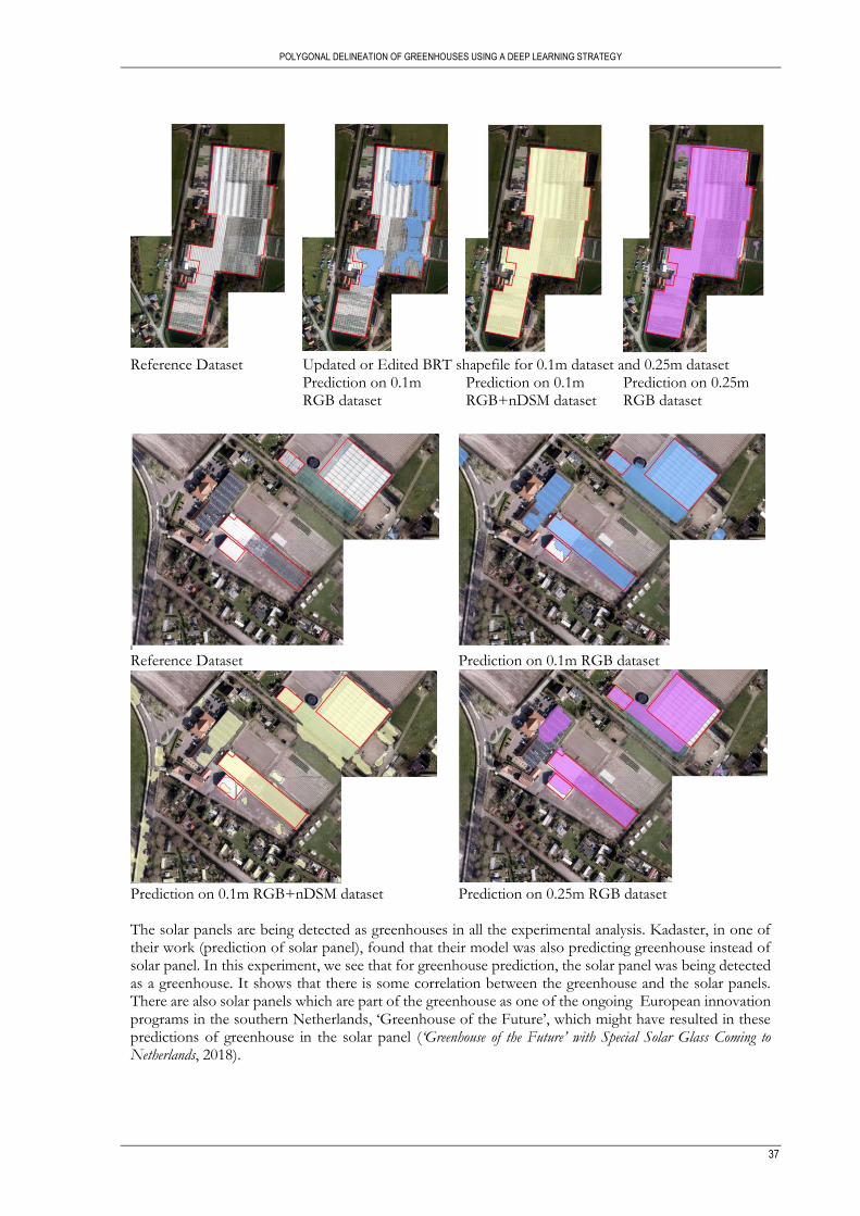
POLYGONAL DELINEATION OF GREENHOUSES USING A DEEP LEARNING STRATEGY
37
Reference Dataset Updated or Edited BRT shapefile for 0.1m dataset and 0.25m dataset Prediction on 0.1m RGB dataset
Prediction on 0.1m RGB+nDSM dataset
Prediction on 0.25m RGB dataset
Reference Dataset Prediction on 0.1m RGB dataset
Prediction on 0.1m RGB+nDSM dataset Prediction on 0.25m RGB dataset The solar panels are being detected as greenhouses in all the experimental analysis. Kadaster, in one of their work (prediction of solar panel), found that their model was also predicting greenhouse instead of solar panel. In this experiment, we see that for greenhouse prediction, the solar panel was being detected as a greenhouse. It shows that there is some correlation between the greenhouse and the solar panels. There are also solar panels which are part of the greenhouse as one of the ongoing European innovation programs in the southern Netherlands, ‘Greenhouse of the Future’, which might have resulted in these predictions of greenhouse in the solar panel (‘Greenhouse of the Future’ with Special Solar Glass Coming to Netherlands, 2018).

POLYGONAL DELINEATION OF GREENHOUSES USING A DEEP LEARNING STRATEGY
38
Reference dataset Prediction on 0.1m RGB dataset
Prediction on 0.1m RGB+nDSM dataset Prediction on 0.25m RGB dataset
Reference Dataset Prediction on 0.1m RGB dataset

POLYGONAL DELINEATION OF GREENHOUSES USING A DEEP LEARNING STRATEGY
39
Prediction on 0.1m RGB+nDSM dataset Prediction on 0.25m RGB dataset
The experimental analysis for the prediction of the polygon of the greenhouse with different tolerance levels
(0.125 pixels, 1 pixel and 9 pixels) is shown in figure 19. For polygonization, as the number of tolerance for
prediction increases, the number of vertices to make the polygon decreases. While the number of tolerance
for prediction decreases, the number of vertices to make the polygon increases.
A predicted polygon with the tolerance of 0.125 pixels for polygonization
Number of vertices = 1468
A predicted polygon with the tolerance of 1 pixel for polygonization
Number of vertices = 674
A predicted polygon with the tolerance of 9 pixels for polygonization
Number of vertices = 395
Figure 19: Example polygon obtained with different tolerance parameters for the polygonization for different band combination
Greenhouses in the Netherlands are mainly made up of glasses, and when aerial images are taken from
aircraft, from the position of the sun and the angle of the flights from which greenhouses were taken, there
will be a reflection of the glass, resulting in greenhouses with different textures and spectral information. In
figure 20, different types of greenhouses in the aerial images are seen: greenhouses are white with a spectral
resolution of value 255 all over the greenhouse, transparent greenhouses that reflect clearly what lies
underneath. One of the reasons for the detection of the white building as the greenhouse was the training
dataset containing white greenhouse, which is the result from the angle from which the image was taken
from the aircraft, making the glass of the greenhouse reflects white, as shown in figure 20.
The method was more effective for the greenhouses made up of glasses than greenhouses made up of
plastic. The reason can be the fewer plastic greenhouses in general. With the addition of nDSM, the plastic

POLYGONAL DELINEATION OF GREENHOUSES USING A DEEP LEARNING STRATEGY
40
greenhouses were predicted, although there was less training dataset due to additional elevational
information.
Figure 20: Greenhouses with different texture
Some greenhouses are transparent, as shown in figure 21, which makes learning during training more
difficult, and rather than learning the spectral and textural features of the greenhouse, it learns the
underneath information.
Figure 21: Transparent greenhouses

POLYGONAL DELINEATION OF GREENHOUSES USING A DEEP LEARNING STRATEGY
41
While acquiring the image of the greenhouse, a certain area within the greenhouse reflects the sun and the
high-intensity reflection values are obtained in that greenhouse, as shown in figure 22. The spectral and the
texture value in that area differs from the, which might have affected the result.
Figure 22: High-intensity reflection in a certain area of the greenhouse while taking an aerial image
6.3. Limitations
The stratification procedure for data preparation might be biased as 50% of the tiles were manually selected
with a greenhouse within them. As the greenhouses are big and occupy large areas ranging from 200 sqm
to 589653.408 sqm, a complete greenhouse would occupy many tiles. The training, testing and validation
tiles were selected such that a complete polygon of the greenhouse lies on one of the three tiles group.
The method of joining the greenhouse that was introduced in section 3.2.2. also has its limitation. The ArcGIS method takes a distance value through which it is buffered. As the method merged and dissolved that predicted polygon together. If the minimal distance between two greenhouses is less than the distance value opted in this method, then the two greenhouses will merge, which will defer the objective of having a single instance of the greenhouse. The model predicts poor results for plastic greenhouses, which can be seen in figure 18. The distribution of plastic greenhouse in the study area is few. The model is biased towards the plastic and glasses greenhouses due to less number of plastic greenhouses.
POLYGONAL DELINEATION OF GREENHOUSES USING A DEEP LEARNING STRATEGY
42
7. CONCLUSION AND RECOMMENDATION
This chapter first describes the conclusion of the overall study and later recommends how to improve the
methodology further.
7.1. Conclusion
A method used to polygonize the building was utilized for polygonization of the greenhouse, which includes
the standard segmentation model with an additional frame field. Adding the nDSM band to the RGB band
resulted in incrementing the accuracy and regularity of prediction. For the bigger objects of interest like
greenhouses, frame field learning was more appropriate for instance segmentation, as the Polymapper
method required to have at least one object of interest with all its boundary within the tiles. The mean IoU
for 0.1 m RGB image was 0.673, while for RGB+ nDSM of 0.1 m dataset was 0.751. Some of the
greenhouses were not predicted in RGB images of 0.1m resolution, while adding nDSM with the RGB
predicted the greenhouse. It concludes that adding nDSM to extract the distinguishes the greenhouses and
the background more accurately. The mean IoU of 0.25 m RGB image was 0.745. The results for 0.25m
datasets were good in some cases, compared to 0.1m datasets, meaning that only resolution of VHR images
cannot only be a factor for better prediction. Greenhouses are big in shape and are visible in both 0.1m and
0.25m datasets. The network can learn spectral and textural features from what is visible from the VHR
imagery. The 0.1m RGB images had more distinct texture features that need to be learned, which might
have resulted in a poor result than the 0.25m datasets for three RGB bands. For 0.1m datasets, the BCE
parameter 0.25 to 0.50 and the Dice coefficient was changed from 0.25 to 0.50, which increases the mean
IoU from 0.675 to 0.784 for three-band RGB images and 0.751 to 0.807 for RGB + nDSM images.
The answers to the research questions of the study are presented below:
RQ1: Which deep learning or CNN architecture is appropriate for automated delineation of
greenhouses in the polygon format?
Frame field learning method was utilized for the delineation of the greenhouses. The model first produced
the classification map by training the deep learning network (UNet-Resnet101) and later vectorised the
classified map. Since the greenhouses to be delineated were big, with an area up to 589653.408 sqm, an
ArcGIS model was introduced to join the greenhouse together.
RQ2: Which cadastral data sets are suitable for the experimental analysis?
Out of the different key registry in the Netherlands, the BRT dataset contained the footprints of the
greenhouse data in the digital format, so the BRT key registry dataset was taken. In terms of images, summer
and winter orthoimages were utilized with the resolution of 0.25m and 0.1m, respectively. The summer
dataset was freely available which could be downloaded from the open government datasets platform,
pdok.nl. The winter orthoimages were private data used for internal uses within the Kadaster. Kadaster took
separate flights to produce the winter orthoimages. For the height data, freely available source, i.e., Actueel
Hoogtebestand Nederland (AHN) data, was not available for the geographical areas within the year of 2019.
So, the nDSM of 2019 with the resolution of 0.2m (which was later resampled for experimental analysis)
was used. The nDSM data was internal data of Kadaster that was obtained from the stereophotogrammetry
process.
RQ3: Does the normalized Digital Surface Model (nDSM) data contribute to more accurate
detection and segmentation of greenhouses?
POLYGONAL DELINEATION OF GREENHOUSES USING A DEEP LEARNING STRATEGY
43
The quantitative result and the qualitative result shows that the addition of nDSM increases the prediction
of greenhouses. The height information contributed to distinguish the greenhouses from the background
more accurately, as shown in figure 17 and 18. For BCE coefficient of 0.25 and Dice coefficient of 0.75, the
mean IoU of 0.1m RGB images was 0.675, and for 0.1m RGB + nDSM images, the mean IoU value
improved to 0.751.
RQ4: What is the effectiveness of the approach for different types of greenhouses (plastics and
glasses)?
The study area with greenhouses had a high number of glasses greenhouses compared to plastic
greenhouses. The training, validation and testing dataset prepared to apply in the frame field method had
more glasses greenhouses, which makes the trained model biased. This is the reason why the prediction of
greenhouse shown in figure 18 had a poor prediction for plastic greenhouses. However, the footprint of
greenhouses on BRT had no separation of plastic or glasses greenhouse. So, only visual inspection was done
to separate the type of greenhouses.
RQ5: Which dataset performs better in terms of delineation of greenhouses?
The height information (nDSM) to the RGB band has increased the prediction of greenhouses compared
to the RGB band. The qualitative analysis shows that out of the combination with the same configuration,
RGB + nDSM showed better performance with the mean IoU value of 0.751.
RQ6: What is the accuracy of the polygonised greenhouse with the standard metrics?
The accuracy of the predicted greenhouse can be seen in table 6 and 7. The mean IoU value was high for
RGB + nDSM dataset with 0.751 for the hyperparameter of 0.25 BCE and 0.75 Dice coefficient. The AP
IoU=0.50:0.05:0.95 value for 0.1m RGB images was greater than the AP IoU=0.50:0.05:0.95 for 0.1m RGB + nDSM with
the value of 0.003, meaning within the threshold from 0.5 to 0.95 with the steps of 0.05, the localization was
better for 0.10m RGB images. Whereas RGB + nDSM for 0.1m images had a high mean AR value,
indicating few false negatives.
RQ7: What are the specification required by Kadaster to update the BRT in terms of the
greenhouse?
The specification required by Kadaster to update the BRT is that the greenhouse is considered to be a
greenhouse when the digital topographic files, in our case greenhouse, should lie in the scale of at least
1:10000 (Ministerie van Binnenlandse Zaken en Koninkrijksrelaties, n.d.-b). The specification to be a
greenhouse was answered by a representative of Kadaster, which is described in section 2.1.3.
RQ8: How can the above technique be used for regular updating of the cadastral database of
greenhouses?
To be able to use the current method for a regular update in the cadastral database of the greenhouse, post-
processing needs to be done. As the predicted greenhouse has more false positives within buildings with
white roofs and solar panels, utilizing the BRT dataset of buildings can help remove the prediction of
greenhouses in buildings with white roofs. Since greenhouses do have solar panels above them, they cannot
be utilized to remove false positives. Manual professional control is required to verify the correctness of the
automatically predicted polygonal greenhouse for updating the cadastral database.
7.2. Recommendation
The proposed methodology can be adopted not only for the objects like a greenhouse but other objects
within the digital objects in BRT. Since the original framework, frame field learning was done for building,

POLYGONAL DELINEATION OF GREENHOUSES USING A DEEP LEARNING STRATEGY
44
other objects such as solar panels and storage tanks have been actively being researched in the object
detection team within Kadaster. The network can be further improved with the fusing strategy of another
layer, such as introducing the nDSM and NIR band for the summer images as an additional layer that might
help contribute to more accurate detection and segmentation. As the deep learning method requires a lot of
ground truth information to train the model, if the method is going to be applied for the whole of the
Netherlands, the training datasets should be significantly increased as only 1.33 sq km of greenhouses are
taken into account. Also, the nature of the greenhouse (transparent glasses and some high-intensity values
within the greenhouse) can be further reviewed.
The parameters of BCE and Dice coefficient can be further checked in terms of greenhouses; as for
buildings, the values of the hyperparameter had good results in 0.25 BCE and 0.75 Dice coefficient value,
whereas for the greenhouse, the values with the hyperparameter of 0.50 BCE and 0.50 Dice coefficient has
increased the accuracy. Further, using the building information, solar panels information, and road
information can be used in post-processing to obtain the greenhouses such that false-positive prediction
can be reduced. Furthermore, different polygonization methods or algorithms should be explored, tested,
analysed, and compared to calculate the applied method’s reliability with other polygonized methods.

45
LIST OF REFERENCES
Agüera, F., Aguilar, M. A., & Aguilar, F. J. (2006). Detecting greenhouse changes from QuickBird imagery
on the Mediterranean coast. International Journal of Remote Sensing, 27(21), 4751–4767. https://doi.org/10.1080/01431160600702681
Agüera, Francisco, Aguilar, F. J., & Aguilar, M. A. (2008a). Using texture analysis to improve per-pixel classification of very high resolution images for mapping plastic greenhouses. ISPRS Journal of Photogrammetry and Remote Sensing, 63(6), 635–646. https://doi.org/10.1016/j.isprsjprs.2008.03.003
Agüera, Francisco, Aguilar, F. J., & Aguilar, M. A. (2008b). Using texture analysis to improve per-pixel classification of very high resolution images for mapping plastic greenhouses. ISPRS Journal of Photogrammetry and Remote Sensing, 63(6), 635–646. https://doi.org/10.1016/j.isprsjprs.2008.03.003
Aguilar, M. A., Saldaña, M. M., & Aguilar, F. J. (2013a). GeoEye-1 and WorldView-2 pan-sharpened imagery for object-based classification in urban environments. International Journal of Remote Sensing, 34(7), 2583–2606. https://doi.org/10.1080/01431161.2012.747018
Aguilar, M. A., Saldaña, M. M., & Aguilar, F. J. (2013b). GeoEye-1 and WorldView-2 pan-sharpened imagery for object-based classification in urban environments. International Journal of Remote Sensing, 34(7), 2583–2606. https://doi.org/10.1080/01431161.2012.747018
Balcik, F. B., Senel, G., & Goksel, C. (2019, July 1). Greenhouse mapping using object based classification and sentinel-2 satellite imagery. 2019 8th International Conference on Agro-Geoinformatics, Agro-Geoinformatics 2019. https://doi.org/10.1109/Agro-Geoinformatics.2019.8820252
Brownlee, J. (2019). A Gentle Introduction to Object Recognition With Deep Learning. Machine Learning Mastery. https://machinelearningmastery.com/object-recognition-with-deep-learning/
Buslaev, A., Seferbekov, S., Iglovikov, V., & Shvets, A. (2018). Fully convolutional network for automatic road extraction from satellite imagery. IEEE Computer Society Conference on Computer Vision and Pattern Recognition Workshops, 2018-June, 207–210. https://doi.org/10.1109/CVPRW.2018.00035
Carrilho, A. C., & Galo, M. (2019). AUTOMATIC OBJECT EXTRACTION FROM HIGH RESOLUTION AERIAL IMAGERY WITH SIMPLE LINEAR ITERATIVE CLUSTERING AND CONVOLUTIONAL NEURAL NETWORKS. ISPRS - International Archives of the Photogrammetry, Remote Sensing and Spatial Information Sciences, XLII-2/W16(2/W16), 61–66. https://doi.org/10.5194/isprs-archives-XLII-2-W16-61-2019
Carvajal, F., Agüera, F., Aguilar, F. J., & Aguilar, M. A. (2010). Relationship between atmospheric corrections and training-site strategy with respect to accuracy of greenhouse detection process from very high resolution imagery. International Journal of Remote Sensing, 31(11), 2977–2994. https://doi.org/10.1080/01431160902946580
Celik, S., & Koc-San, D. (2019a). Greenhouse Detection from Color Infrared Aerial Image and Digital Surface Model. Proceedings of 6th International Electronic Conference on Sensors and Applications, 42(1), 6548. https://doi.org/10.3390/ecsa-6-06548
Celik, S., & Koc-San, D. (2019b). Greenhouse Detection from Color Infrared Aerial Image and Digital Surface Model. Proceedings of 6th International Electronic Conference on Sensors and Applications, 42(1), 6548. https://doi.org/10.3390/ecsa-6-06548
Celik, S., & Koc-San, D. (2018). Greenhouse detection using aerial orthophoto and digital surface model. Smart Innovation, Systems and Technologies, 76, 51–59. https://doi.org/10.1007/978-3-319-59480-4_6
Chen, K., Pang, J., Wang, J., Xiong, Y., Li, X., Sun, S., Feng, W., Liu, Z., Shi, J., Ouyang, W., Loy, C. C., & Lin, D. (2019). Hybrid Task Cascade for Instance Segmentation. Proceedings of the IEEE Computer Society Conference on Computer Vision and Pattern Recognition, 2019-June, 4969–4978. http://arxiv.org/abs/1901.07518
Cheng, G., Han, J., & Lu, X. (2017). Remote Sensing Image Scene Classification: Benchmark and State of the Art. In Proceedings of the IEEE (Vol. 105, Issue 10, pp. 1865–1883). Institute of Electrical and Electronics Engineers Inc. https://doi.org/10.1109/JPROC.2017.2675998
COCO - Common Objects in Context. (n.d.). COCO. Retrieved August 6, 2021, from https://cocodataset.org/#detection-eval
Digitaleoverheid.nl. (n.d.). Key Register Large-Scale Topography (BGT). Retrieved September 21, 2020, from https://www.digitaleoverheid.nl/overzicht-van-alle-onderwerpen/basisregistraties-en-stelselafspraken/inhoud-basisregistraties/bgt/
Gandhi, R. (2018). R-CNN , Fast R-CNN , Faster R-CNN , YOLO — Object Detection Algorithms

46
Understanding object detection algorithms R-CNN. Medium, 1–11. https://towardsdatascience.com/r-cnn-fast-r-cnn-faster-r-cnn-yolo-object-detection-algorithms-36d53571365e
Girard, N., Smirnov, D., Solomon, J., & Tarabalka, Y. (2020). Regularized building segmentation by frame field learning. IEEE International Geoscience and Remote Sensing Symposium. https://doi.org/10.1109/IGARSS39084.2020.9324080
Girard, N., Smirnov, D., Solomon, J., & Tarabalka, Y. (2021). Polygonal building extraction by frame field learning. https://github.com/Lydorn/
Girshick, R., Donahue, J., Darrell, T., & Malik, J. (2014). Rich feature hierarchies for accurate object detection and semantic segmentation. Proceedings of the IEEE Computer Society Conference on Computer Vision and Pattern Recognition, 580–587. https://doi.org/10.1109/CVPR.2014.81
González-Yebra, Ó., Aguilar, M. A., Nemmaoui, A., & Aguilar, F. J. (2018). Methodological proposal to assess plastic greenhouses land cover change from the combination of archival aerial orthoimages and Landsat data. Biosystems Engineering, 175, 36–51. https://doi.org/10.1016/j.biosystemseng.2018.08.009
Government.nl. (n.d.). Municipalities’ tasks. Retrieved October 12, 2020, from https://www.government.nl/topics/municipalities/municipalities-tasks
‘Greenhouse of the Future’ with special solar glass coming to Netherlands. (2018). Horti Daily. https://www.hortidaily.com/article/6042937/greenhouse-of-the-future-with-special-solar-glass-coming-to-netherlands/
He, K., Gkioxari, G., Dollár, P., & Girshick, R. (2020). Mask R-CNN. IEEE Transactions on Pattern Analysis and Machine Intelligence, 42(2), 386–397. https://doi.org/10.1109/TPAMI.2018.2844175
Hemmati, M. (2002). Multi-stakeholder Processes for Governance and Sustainability. Earthscan Publications Ltd. Hoeser, T., & Kuenzer, C. (2020). Object Detection and Image Segmentation with Deep Learning on
Earth Observation Data: A Review-Part I: Evolution and Recent Trends. Remote Sensing, 12(10), 1667. https://doi.org/10.3390/rs12101667
Iglovikov, V., Seferbekov, S., Buslaev, A., & Shvets, A. (2018). TernausNetV2: Fully convolutional network for instance segmentation. IEEE Computer Society Conference on Computer Vision and Pattern Recognition Workshops, 2018-June, 228–232. https://doi.org/10.1109/CVPRW.2018.00042
Information about the Register of Large-scale Topography (BGT) - Land Registry business. (n.d.). Retrieved June 16, 2020, from https://zakelijk.kadaster.nl/bgt
Ji, S., Shen, Y., Lu, M., & Zhang, Y. (2019). Building Instance Change Detection from Large-Scale Aerial Images using Convolutional Neural Networks and Simulated Samples. Remote Sensing, 11(11), 1343. https://doi.org/10.3390/rs11111343
Kadaster. (n.d.-a). About us - Kadaster. Retrieved October 12, 2020, from https://www.kadaster.com/about-kadaster
Kadaster. (n.d.-b). Dataset: Aerial / PDOK (Open). PDOK. Retrieved August 20, 2021, from https://www.pdok.nl/introductie/-/article/luchtfoto-pdok
Kadaster. (n.d.-c). Key Register Large-Scale Topography (BGT). Retrieved September 21, 2020, from https://www.kadaster.nl/zakelijk/registraties/basisregistraties/bgt
Kadaster. (n.d.-d). TOP10NL - Product information - Land Registry business. Kadaster. (2020). Basisregistratie Topografie: Catalogus en Productspecificaties.
https://www.kadaster.nl/documents/1953498/2762084/BRT+catalogus+productspecificaties.pdf/8d315269-a40f-819c-6a58-7e85b59b6718?t=1588864445108
Kaiser, P., Wegner, J. D., Lucchi, A., Jaggi, M., Hofmann, T., & Schindler, K. (2017). Learning Aerial Image Segmentation from Online Maps. IEEE Transactions on Geoscience and Remote Sensing, 55(11), 6054–6068. https://doi.org/10.1109/TGRS.2017.2719738
Key Register Topography (BRT). (n.d.). Retrieved September 23, 2020, from https://www.kadaster.nl/zakelijk/registraties/basisregistraties/brt
Koc-San, D., & Sonmez, N. K. (2016). Plastic and glass greenhouses detection and delineation from Worldview - 2 Satellite Imagery. ISPRS - International Archives of the Photogrammetry, Remote Sensing and Spatial Information Sciences, XLI-B7, 257–262. https://doi.org/10.5194/isprs-archives-xli-b7-257-2016
Koc-San, Dilek. (2013a). Evaluation of different classification techniques for the detection of glass and plastic greenhouses from WorldView-2 satellite imagery. Journal of Applied Remote Sensing, 7(1), 073553. https://doi.org/10.1117/1.jrs.7.073553
Koc-San, Dilek. (2013b). Evaluation of different classification techniques for the detection of glass and plastic greenhouses from WorldView-2 satellite imagery. Journal of Applied Remote Sensing, 7(1),

47
073553. https://doi.org/10.1117/1.jrs.7.073553 Krizhevsky, A., Sutskever, I., & Hinton, G. E. (2012). ImageNet Classification with Deep Convolutional
Neural Networks. In Advances in Neural Information Processing Systems, 25(Pereira, F., Burges, C.J.C., Bottou, L., Weinberger, K.Q., Eds.; Curran Associates; Red Hook, NY, USA,), 1097–1105. https://papers.nips.cc/paper/4824-imagenet-classification-with-deep-convolutional-neural-networks.pdf
Li, M., Lafarge, F., & Marlet, R. (2020). Approximating shapes in images with low-complexity polygons. Proceedings of the IEEE Computer Society Conference on Computer Vision and Pattern Recognition, 8630–8638. https://doi.org/10.1109/CVPR42600.2020.00866
Li, Z., Wegner, J. Di., & Lucchi, A. (2019). Topological map extraction from overhead images. Proceedings of the IEEE International Conference on Computer Vision, 2019-October, 1715–1724. https://doi.org/10.1109/ICCV.2019.00180
Ling, H., Gao, J., Kar, A., Chen, W., & Fidler, S. (2019). Fast Interactive Object Annotation with Curve-GCN. Proceedings of the IEEE Computer Society Conference on Computer Vision and Pattern Recognition, 2019-June, 5252–5261. https://arxiv.org/abs/1903.06874v1
Liu, P. L. (2020). Single Stage Instance Segmentation — A Review. Towards Data Science. https://towardsdatascience.com/single-stage-instance-segmentation-a-review-1eeb66e0cc49
Liu, S., Qi, L., Qin, H., Shi, J., & Jia, J. (2018). Path Aggregation Network for Instance Segmentation. Proceedings of the IEEE Computer Society Conference on Computer Vision and Pattern Recognition, 8759–8768. https://doi.org/10.1109/CVPR.2018.00913
Long, J., Shelhamer, E., & Darrell, T. (2015). Fully convolutional networks for semantic segmentation. Proceedings of the IEEE Computer Society Conference on Computer Vision and Pattern Recognition, 07-12-June-2015, 3431–3440. https://doi.org/10.1109/CVPR.2015.7298965
Lorensen, W. E., & Cline, H. E. (1987). MARCHING CUBES: A HIGH RESOLUTION 3D SURFACE CONSTRUCTION ALGORITHM. Proceedings of the 14th Annual Conference on Computer Graphics and Interactive Techniques - SIGGRAPH ’87, 21(4). https://doi.org/10.1145/37401
Ministerie van Binnenlandse Zaken en Koninkrijksrelaties. (n.d.-a). Key Register Large-Scale Topography. Retrieved September 13, 2020, from https://www.geobasisregistraties.nl/basisregistraties/bgt/basisregistratie-grootschalige-topografie
Ministerie van Binnenlandse Zaken en Koninkrijksrelaties. (n.d.-b). Key Register Topography. Geo Basic Registrations | The Geobasic Registrations. Retrieved August 9, 2021, from https://www.geobasisregistraties.nl/basisregistraties/topografie
Ministerie Van Binnenlandse Zaken en Koninkrijksrelaties. (n.d.). The geobasic registrations. Geo Basic Registrations. Retrieved August 9, 2021, from https://www.geobasisregistraties.nl/basisregistraties
Montoya-Zegarra, J. A., Wegner, J. D., Ladický, L., & Schindler, K. (2015). Semantic Segmentation of Aerial Imges in Urban Areas with class-specific higher order cliques. ISPRS Annals of Photogrammetry, Remote Sensing and Spatial Information Sciences, II-3/W4(3W4), 127–133. https://doi.org/10.5194/isprsannals-II-3-W4-127-2015
Novelli, A., Aguilar, M. A., Nemmaoui, A., Aguilar, F. J., & Tarantino, E. (2016). Performance evaluation of object based greenhouse detection from Sentinel-2 MSI and Landsat 8 OLI data: A case study from Almería (Spain). International Journal of Applied Earth Observation and Geoinformation, 52, 403–411. https://doi.org/10.1016/j.jag.2016.07.011
Pan, X., Yang, F., Gao, L., Chen, Z., Zhang, B., Fan, H., & Ren, J. (2019). Building extraction from high-resolution aerial imagery using a generative adversarial network with spatial and channel attention mechanisms. Remote Sensing, 11(8). https://doi.org/10.3390/rs11080966
Potlapally, A., Chowdary, P. S. R., Raja Shekhar, S. S., Mishra, N., Madhuri, C. S. V. D., & Prasad, A. V. V. (2019). Instance Segmentation in Remote Sensing Imagery using Deep Convolutional Neural Networks. Proceedings of the 4th International Conference on Contemporary Computing and Informatics, IC3I 2019, 117–120. https://doi.org/10.1109/IC3I46837.2019.9055569
Ramer, U. (1972). An iterative procedure for the polygonal approximation of plane curves. Computer Graphics and Image Processing, 1(3), 244–256. https://doi.org/10.1016/S0146-664X(72)80017-0
Saito, S., & Aoki, Y. (2015). Building and road detection from large aerial imagery. In E. Y. Lam & K. S. Niel (Eds.), Image Processing: Machine Vision Applications VIII (Vol. 9405, p. 94050K). SPIE. https://doi.org/10.1117/12.2083273
Shi, L., Huang, X., Zhong, T., & Taubenbock, H. (2020). Mapping Plastic Greenhouses Using Spectral Metrics Derived from GaoFen-2 Satellite Data. IEEE Journal of Selected Topics in Applied Earth Observations and Remote Sensing, 13, 49–59. https://doi.org/10.1109/JSTARS.2019.2950466

48
Shrestha, S., & Vanneschi, L. (2018). Improved Fully Convolutional Network with Conditional Random Fields for Building Extraction. Remote Sensing, 10(7), 1135. https://doi.org/10.3390/rs10071135
Su, H., Wei, S., Yan, M., Wang, C., Shi, J., & Zhang, X. (2019). Object Detection and Instance Segmentation in Remote Sensing Imagery Based on Precise Mask R-CNN. International Geoscience and Remote Sensing Symposium (IGARSS), 1454–1457. https://doi.org/10.1109/IGARSS.2019.8898573
Tarantino, E., & Figorito, B. (2012). Mapping Rural Areas with Widespread Plastic Covered Vineyards Using True Color Aerial Data. Remote Sensing, 4(7), 1913–1928. https://doi.org/10.3390/rs4071913
Tayara, H., & Chong, K. (2018). Object Detection in Very High-Resolution Aerial Images Using One-Stage Densely Connected Feature Pyramid Network. Sensors, 18(10), 3341. https://doi.org/10.3390/s18103341
Tiu, E. (2019). Metrics to Evaluate your Semantic Segmentation Model. Towards Data Science. https://towardsdatascience.com/metrics-to-evaluate-your-semantic-segmentation-model-6bcb99639aa2
Tiwari, K. N. (n.d.). MI&CAD: Lesson 29. Classification of Greenhouse. Zhao, K., Kamran, M., & Sohn, G. (2020). BOUNDARY REGULARIZED BUILDING FOOTPRINT
EXTRACTION FROM SATELLITE IMAGES USING DEEP NEURAL NETWORKS. ISPRS Annals of Photogrammetry, Remote Sensing and Spatial Information Sciences, V-2–2020(2), 617–624. https://doi.org/10.5194/isprs-annals-V-2-2020-617-2020
Zhao, W., Ivanov, I., Persello, C., & Stein, A. (2020). BUILDING OUTLINE DELINEATION: FROM VERY HIGH RESOLUTION REMOTE SENSING IMAGERY TO POLYGONS WITH AN IMPROVED END-TO-END LEARNING FRAMEWORK. ISPRS - International Archives of the Photogrammetry, Remote Sensing and Spatial Information Sciences, XLIII-B2-2, 731–735. https://doi.org/10.5194/isprs-archives-xliii-b2-2020-731-2020
Zhao, W., Persello, C., & Stein, A. (2021). Building outline delineation: From aerial images to polygons with an improved end-to-end learning framework. ISPRS Journal of Photogrammetry and Remote Sensing, 175, 119–131. https://doi.org/10.1016/J.ISPRSJPRS.2021.02.014
Zorzi, S., & Fraundorfer, F. (2020). Regularization of Building Boundaries in Satellite Images using Adversarial and Regularized Losses. 5140–5143. https://arxiv.org/abs/2007.11840v1