Embed Size (px)
Citation preview
Filippo GazzolaHans-Christoph GrunauGuido Sweers
Polyharmonic boundary valueproblems
A monograph on positivity preserving andnonlinear higher order elliptic equations inbounded domains
Springer
Dedicated to our wives Chiara, Brigitte and Barbara.
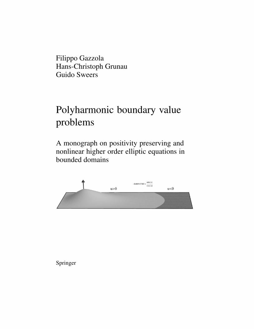
The cover figure displays the solution of ∆ 2u = f in a rectangle with homogeneousDirichlet boundary condition for a nonnegative function f with its support concen-trated near a point on the left hand side. The dark part shows the region where u < 0.
Preface
Linear elliptic equations arise in several models describing various phenomena inthe applied sciences, the most famous being the second order stationary heat equa-tion or, equivalently, the membrane equation. For this intensively well-studied linearproblem there are two main lines of results. The first line consists of existence andregularity results. Usually the solution exists and “gains two orders of differenti-ation” with respect to the source term. The second line contains comparison typeresults, namely the property that a positive source term implies that the solutionis positive under suitable side constraints such as homogeneous Dirichlet bound-ary conditions. This property is often also called positivity preserving or, simply,maximum principle. These kinds of results hold for general second order ellipticproblems, see the books by Gilbarg-Trudinger [197] and Protter-Weinberger [346].For linear higher order elliptic problems the existence and regularity type results re-main, as one may say, in their full generality whereas comparison type results mayfail. Here and in the sequel “higher order” means order at least four.
Most interesting models, however, are nonlinear. By now, the theory of secondorder elliptic problems is quite well developed for semilinear, quasilinear and evenfor some fully nonlinear problems. If one looks closely at the tools being used inthe proofs, then one finds that many results benefit in some way from the positivitypreserving property. Techniques based on Harnack’s inequality, De Giorgi-Nash-Moser’s iteration, viscosity solutions etc., all use suitable versions of a maximumprinciple. This is a crucial distinction from higher order problems for which there isno obvious positivity preserving property. A further crucial tool related to the max-imum principle and intensively used for second order problems is the truncationmethod, introduced by Stampacchia. This method is helpful in regularity theory, inproperties of first order Sobolev spaces and in several geometric arguments, suchas the moving planes technique which proves symmetry of solutions by reflection.Also the truncation (or reflection) method fails for higher order problems. For in-stance, the modulus of a function belonging to a second order Sobolev space maynot belong to the same space. The failure of maximum principles and of truncationmethods, one could say, are the main reasons why the theory of nonlinear higherorder elliptic equations is by far less developed than the theory of analogous second
v
vi Preface
order equations. On the other hand, in view of many applications and increasing in-terest especially in the last twenty years, one should try to develop new tools suitablefor higher order problems involving polyharmonic operators.
The simple example of the two functions x 7→±|x|2 shows that already for the bi-harmonic operator the standard maximum principle fails. Nevertheless, taking alsoboundary conditions into account could yield comparison or positivity preservingproperties and indeed, in certain special situations, such behaviour can be observed.It is one goal of the present exposition to describe situations where positivity pre-serving properties hold true or fail, respectively, and to explain how we have tackledthe main difficulties related to the lack of a general comparison principle. In thepresent book we also show that in many higher order problems positivity preserving“almost” occurs. By this we mean that the solution to a problem inherits the signof the data, except for some small contribution. By the experience from the presentwork, we hope that suitable techniques may be developed in order to obtain resultsquite analogous to the second order situation. Many recent higher order results givesupport to this hope.
A further goal of the present book is to collect some of those problems, where theauthors were particularly involved, and to explain by which new methods one canreplace second order techniques. In particular, to overcome the failure of the maxi-mum principle and of the truncation method several ad hoc ideas will be introduced.
Let us now explain in some detail the subjects we address within this book.
Linear higher order elliptic problems
The polyharmonic operator (−∆)m is the prototype of an elliptic operator L of order2m, but with respect to linear questions, much more general operators can be con-sidered. A general theory for boundary value problems for linear elliptic operatorsL of order 2m was developed by Agmon-Douglis-Nirenberg [4, 5, 6, 148]. Althoughthe material is quite technical, it turns out that the Schauder theory as well as theLp-theory can be developed to a large extent analogously to second order equations.The only exception are maximum modulus estimates which, for linear higher orderproblems, are much more restrictive than for second order problems. We provide asummary of the main results which hopefully will prove to be sufficiently wide tobe useful for anybody who needs to refer to linear estimates or existence results.
The main properties of higher – at least second – order Sobolev spaces will berecalled. Since more orders of differentiation are involved, several different equiv-alent norms are available in these spaces. A crucial role in the choice of the normis played by the regularity of the boundary. For the second order Dirichlet problemfor the Poisson equation a nonsmooth boundary leads to technical difficulties but,due to the maximum principle, there is an inherent stability so that, when approxi-mating nonsmooth domains by smooth domains, one recovers most of the featuresfor domains with smooth boundary, see [46]. For Neumann boundary conditionsthe situation is more complicated in domains with rather wild boundaries, although
Preface vii
even for polygonal boundaries they do not show spectacular changes. For higherorder boundary value problems some peculiar phenomena occur. For instance, theso-called Babuska and Sapondzyan paradoxes [28, 357] forces one to be very care-ful in the choice of the norm in second order Sobolev spaces since some boundaryvalue problems strongly depend on the regularity of the boundary. This phenomenonand its consequences will be studied in some detail.
Positivity in higher order elliptic problems
As long as existence and regularity results are concerned, the theory of linear higherorder problems is already quite well developed as explained above. This is no longertrue as soon as qualitative properties of the solution related to the source term areinvestigated. For instance, if we consider the clamped plate equation
∆ 2u = f in Ω ,
u = ∂u∂ν
= 0 on ∂Ω ,(0.1)
the “simplest question” seems to find out whether the positivity of the datum impliesthe positivity of the solution, Or, physically speaking,
does upwards pushing of a clamped plate yield upwards bending?
Equivalently, one may ask whether the corresponding Green function G is positive.In some special cases, the answer is “yes”, while it is “no” in general. However,in numerical experiments, it appears very difficult to display the negative part andheuristically, one feels that the negative part of G – if present at all – is small in asuitable sense compared with the “dominating” positive part. We discuss not onlythe cases where one has positive Green functions and develop a perturbation theoryof positivity, but we shall also discuss systematically under which conditions onemay expect the negative part of the Green function to be small. We expect suchsmallness results to have some impact on future developments in the theory of non-linear higher order elliptic boundary value problems.
Boundary conditions
For second order elliptic equations one usually extensively studies the case ofDirichlet boundary conditions because other boundary conditions do not exhibittoo different behaviours. For the biharmonic equation ∆ 2u = f in a bounded do-main of Rn it is not at all obvious which boundary condition would serve as a rolemodel. Then a good approach is to focus on some boundary conditions that describephysically relevant situations. We consider a simplified energy functional and de-rive its Euler-Lagrange equation including the corresponding natural boundary con-ditions. We start with the linearised model for the beam. From a physical point of
viii Preface
view, as long as the fourth order planar equation is considered, the most interest-ing seem to be not only the Dirichlet boundary conditions but also the Navier orSteklov boundary conditions. The Dirichlet conditions correspond to the clampedplate model whereas Navier and Steklov conditions correspond to the hinged platemodel, either by neglecting or considering the contribution of the curvature of theboundary. Each one of these boundary conditions requires the unknown functionto vanish on the boundary, the difference being on the second boundary condition.These three boundary conditions have their own features and none of them may bethought to play the model role. We discuss all of them and emphasise their own pe-culiarities with respect to the comparison principles, to their variational formulationand to solvability of related nonlinear problems.
Eigenvalue problems
For second order problems, such as the Dirichlet problem for the Laplace operator,one has not only the existence of infinitely many eigenvalues but also the simplicityand the one sign property of the first eigenfunction. For the biharmonic Dirichletproblem, this property is true in a ball but it is false in general. Again, a crucial roleis played by the sign of the corresponding Green function. Concerning the isoperi-metric properties of the first eigenvalue of the Dirichlet-Laplacian, the Faber-Krahn[162, 253, 254] result states that, among domains having the same finite volume itattains its minimum when the domain is a ball. A similar result was conjectured tohold for the biharmonic operator under homogeneous Dirichlet boundary conditionsby Lord Rayleigh [350] in 1894. Although this statement has been proved only indomains of dimensions n = 2,3, it is the common feeling that it should be true inany dimension. The minimisation of the first Steklov eigenvalue appears to be lessobvious. And, indeed, we will see that a Faber-Krahn type result does not hold inthis case.
Semilinear equations
Among nonlinear problems for higher order elliptic equations one may just mentionmodels for thin elastic plates, stationary surface diffusion flow, the Paneitz-Bransonequation and the Willmore equation as frequently studied. In membrane biophysicsthe Willmore equation is also known as Helfrich model [227]. Moreover, severalresults concerning semilinear equations with power type nonlinear sources are alsoextremely useful in order to understand interesting phenomena in functional analysissuch as the failure of compactness in the critical Sobolev embedding and in relatedinequalities.
One further motivation to study nonlinear higher order elliptic reaction-diffusiontype equations like

Preface ix
(−∆)mu = f (u) (∗)
in bounded domains is to understand whether the results available in the simplestcase m = 1 can also be proved for any m, or whether the results for m = 1 are special,in particular as far as positivity and the use of maximum principles are concerned.The differential equation (∗) is complemented with suitable boundary conditions. Asalready mentioned above, if m = n = 2, equation (∗) may be considered as a non-linear plate equation for plates subject to nonlinear feedback forces, one may thinke.g. of suspension bridges. In this case, (∗) may also be interpreted as a reaction-diffusion equation, where the diffusion operator ∆ 2 refers to (linearised) surfacediffusion.
The first part of Chapter 7 is devoted to the proof of symmetry results for pos-itive solutions to (∗) in the ball under Dirichlet boundary conditions. As alreadymentioned, truncation and reflection methods do not apply to higher order problemsso that a suitable generalisation of the moving planes technique is needed here.
Equation (∗) deserves a particular attention when f (u) has a power-type be-haviour. In this case, a crucial role is played by the critical power s = (n+2m)/(n−2m) which corresponds to the critical (Sobolev) exponent which appears whenevern > 2m. Indeed, subcritical problems in bounded domains enjoy compactness prop-erties as a consequence of the Rellich-Kondrachov embedding theorem. But com-pactness is lacking when the critical growth is attained and by means of Pohozaev-type identities, this gives rise to many interesting phenomena. The existence theorycan be developed similarly to the second order case m = 1 while it becomes im-mediately quite difficult to prove positivity or nonexistence of certain solutions.Nonexistence phenomena are related to so-called critical dimensions introduced byPucci-Serrin [347, 348]. They formulated an interesting conjecture concerning thesecritical dimensions. We give a proof of a relaxed form of it in Chapter 7. We alsogive a functional analytic interpretation of these nonexistence results, which is re-flected in the possibility of adding L2–remainder terms in Sobolev inequalities withcritical exponent and optimal constants. Moreover, the influence of topological andgeometrical properties of Ω on the solvability of the equation is investigated. Alsoapplications to conformal geometry, such as the Paneitz-Branson equation, involvethe critical Sobolev exponent since the corresponding semilinear equation enjoysa conformal covariance property. In this context a key role is played by a fourthorder curvature invariant, the so-called Q-curvature. Our book does not aim at giv-ing an overview of this rapidly developing subject. For this purpose we refer to themonographs of Chang [89] and Druet-Hebey-Robert [149]. We want to put a spoton some special aspects of such kind of equations. First, we consider the questionwhether in suitable domains in euclidean space it is possible to change the euclideanbackground metric conformally into a metric which has strictly positive constant Q-curvature, while at the same time, certain geometric quantities vanish on the bound-ary. Secondly, we study a phenomenon of nonuniqueness of complete metrics in hy-perbolic space, all being conformal to the Poincare-metric and all having the sameconstant Q-curvature. This result is in strict contrast with the corresponding probleminvolving constant negative scalar curvature.
x Preface
We conclude the discussion of semilinear elliptic problems with some obser-vations on fourth order problems with supercritical growth. Corresponding secondorder results heavily rely on the use of maximum principles and constructions ofmany refined auxiliary functions having some sub- or supersolution property. Suchtechniques are not available at all for the fourth order problems. In symmetric situa-tions, however, they could be replaced by different tools so that many of the resultsbeing well established for second order equations do indeed carry over to the fourthorder ones.
A Dirichlet problem for Willmore surfaces of revolution
A frame invariant modeling of elastic deformations of surfaces like thin plates orbiological membranes gives rise to variational integrals involving curvature and areaterms. A special case is the Willmore functional∫
Γ
H2 dω,
which up to a boundary term is conformally invariant. Here H denotes the meancurvature of the surface Γ in R3. Critical points of this functional are calledWillmore surfaces, the corresponding Euler-Lagrange equation is the so-calledWillmore equation. It is quasilinear, of fourth order and elliptic. While a num-ber of beautiful results have been recently found for closed surfaces, see e.g.[35, 156, 262, 263, 264, 371], only little is known so far about boundary value prob-lems since the difficulties mentioned earlier being typical for fourth order problemsdue to a lack of maximum principles add here to the difficulty that the ellipticityof the equation is not uniform. The latter reflects the geometric nature of the equa-tion and gives rise e.g. to the problem that minimising sequences for the Willmorefunctional are in general not bounded in the Sobolev space H2. In this book weconfine ourselves to a very special situation, namely the Dirichlet problem for sym-metric Willmore surfaces of revolution. Here, by means of some refined geometricconstructions, we succeed in considering minimising sequences of the Willmorefunctional subject to Dirichlet boundary conditions and with suitable additional C1-properties thereby gaining weak H2- and strong C1-compactness. We expect thetheory of boundary value problems for Willmore surfaces to develop rapidly andconsider this chapter as one contribution to outline directions of possible future re-search in quasilinear geometric fourth order equations.
Acknowledgements
The authors are grateful to their colleagues, friends, and collaborators Gianni Ar-ioli, Elvise Berchio, Francisco Bernis, Isabeau Birindelli, Dorin Bucur, DanieleCassani, Philippe Clement, Anna Dall’Acqua, Cesare Davini, Klaus Deckelnick,Alberto Ferrero, Steffen Frohlich, Maurizio Grasselli, Gerhard Huisken, PaschalisKarageorgis, Bernd Kawohl, Marco Kuhnel, Ernst Kuwert, Monica Lazzo, AndreaMalchiodi, Joseph McKenna, Christian Meister, Erich Miersemann, Enzo Mitidieri,Serguei Nazarov, Mohameden Ould Ahmedou, Vittorino Pata, Dario Pierotti, Wolf-gang Reichel, Frederic Robert, Bernhard Ruf, Edoardo Sassone, Reiner Schatzle,Friedhelm Schieweck, Paul G. Schmidt, Marco Squassina, Franco Tomarelli, Wolfvon Wahl, and Tobias Weth for inspiring discussions and sharing ideas.
Essential parts of the book are based on work published in different form before.We thank our numerous collaborators for their contributions. Detailed informationon the sources are given in the bibliographical notes at the end of each chapter.
And last but not least, we thank the referees for their helpful and encouragingcomments.
xi

Contents
Preface . . . . . . . . . . . . . . . . . . . . . . . . . . . . . . . . . . . . . . . . . . . . . . . . . . . . . . . . . . . . v
Acknowledgements . . . . . . . . . . . . . . . . . . . . . . . . . . . . . . . . . . . . . . . . . . . . . . . . . xi
1 Models of higher order . . . . . . . . . . . . . . . . . . . . . . . . . . . . . . . . . . . . . . . . . 11.1 Classical problems from elasticity . . . . . . . . . . . . . . . . . . . . . . . . . . . . . 1
1.1.1 The static loading of a slender beam . . . . . . . . . . . . . . . . . . . . 21.1.2 The Kirchhoff-Love model for a thin plate . . . . . . . . . . . . . . . 51.1.3 Decomposition into second order systems . . . . . . . . . . . . . . . . 7
1.2 The Boggio-Hadamard conjecture for a clamped plate . . . . . . . . . . . . 91.3 The first eigenvalue . . . . . . . . . . . . . . . . . . . . . . . . . . . . . . . . . . . . . . . . . 12
1.3.1 The Dirichlet eigenvalue problem . . . . . . . . . . . . . . . . . . . . . . . 131.3.2 An eigenvalue problem for a buckled plate . . . . . . . . . . . . . . . 131.3.3 A Steklov eigenvalue problem . . . . . . . . . . . . . . . . . . . . . . . . . 15
1.4 Paradoxes for the hinged plate . . . . . . . . . . . . . . . . . . . . . . . . . . . . . . . . 161.4.1 Sapondzyan’s paradox by concave corners . . . . . . . . . . . . . . . 161.4.2 The Babuska paradox . . . . . . . . . . . . . . . . . . . . . . . . . . . . . . . . . 17
1.5 Paneitz-Branson type equations . . . . . . . . . . . . . . . . . . . . . . . . . . . . . . . 181.6 Critical growth polyharmonic model problems . . . . . . . . . . . . . . . . . . 201.7 Qualitative properties of solutions to semilinear problems . . . . . . . . . 221.8 Willmore surfaces . . . . . . . . . . . . . . . . . . . . . . . . . . . . . . . . . . . . . . . . . . 23
2 Linear problems . . . . . . . . . . . . . . . . . . . . . . . . . . . . . . . . . . . . . . . . . . . . . . . 252.1 Polyharmonic operators . . . . . . . . . . . . . . . . . . . . . . . . . . . . . . . . . . . . . 252.2 Higher order Sobolev spaces . . . . . . . . . . . . . . . . . . . . . . . . . . . . . . . . . 27
2.2.1 Definitions and basic properties . . . . . . . . . . . . . . . . . . . . . . . . 272.2.2 Embedding theorems . . . . . . . . . . . . . . . . . . . . . . . . . . . . . . . . . 30
2.3 Boundary conditions . . . . . . . . . . . . . . . . . . . . . . . . . . . . . . . . . . . . . . . . 312.4 Hilbert space theory . . . . . . . . . . . . . . . . . . . . . . . . . . . . . . . . . . . . . . . . 34
2.4.1 Normal boundary conditions and Green’s formula . . . . . . . . . 342.4.2 Homogeneous boundary value problems . . . . . . . . . . . . . . . . . 36
xiii
xiv Contents
2.4.3 Inhomogeneous boundary value problems . . . . . . . . . . . . . . . . 402.5 Regularity results and a priori estimates . . . . . . . . . . . . . . . . . . . . . . . . 42
2.5.1 Schauder theory . . . . . . . . . . . . . . . . . . . . . . . . . . . . . . . . . . . . . 422.5.2 Lp-theory . . . . . . . . . . . . . . . . . . . . . . . . . . . . . . . . . . . . . . . . . . . 442.5.3 The Miranda-Agmon maximum modulus estimates . . . . . . . . 46
2.6 Green’s function and Boggio’s formula . . . . . . . . . . . . . . . . . . . . . . . . 472.7 The space H2∩H1
0 and the Sapondzyan-Babuska paradoxes . . . . . . . 492.8 Bibliographical notes . . . . . . . . . . . . . . . . . . . . . . . . . . . . . . . . . . . . . . . 57
3 Eigenvalue problems . . . . . . . . . . . . . . . . . . . . . . . . . . . . . . . . . . . . . . . . . . . 593.1 Dirichlet eigenvalues . . . . . . . . . . . . . . . . . . . . . . . . . . . . . . . . . . . . . . . . 60
3.1.1 A generalised Kreın-Rutman result . . . . . . . . . . . . . . . . . . . . . 603.1.2 Decomposition with respect to dual cones . . . . . . . . . . . . . . . . 613.1.3 Positivity of the first eigenfunction . . . . . . . . . . . . . . . . . . . . . . 663.1.4 Symmetrisation and Talenti’s comparison principle . . . . . . . . 693.1.5 The Rayleigh conjecture for the clamped plate . . . . . . . . . . . . 71
3.2 Buckling load of a clamped plate . . . . . . . . . . . . . . . . . . . . . . . . . . . . . 753.3 Steklov eigenvalues . . . . . . . . . . . . . . . . . . . . . . . . . . . . . . . . . . . . . . . . . 80
3.3.1 The Steklov spectrum . . . . . . . . . . . . . . . . . . . . . . . . . . . . . . . . 813.3.2 Minimisation of the first eigenvalue . . . . . . . . . . . . . . . . . . . . . 87
3.4 Bibliographical notes . . . . . . . . . . . . . . . . . . . . . . . . . . . . . . . . . . . . . . . 93
4 Kernel estimates . . . . . . . . . . . . . . . . . . . . . . . . . . . . . . . . . . . . . . . . . . . . . . . 974.1 Consequences of Boggio’s formula . . . . . . . . . . . . . . . . . . . . . . . . . . . . 974.2 Kernel estimates in the ball . . . . . . . . . . . . . . . . . . . . . . . . . . . . . . . . . . 99
4.2.1 Direct Green function estimates . . . . . . . . . . . . . . . . . . . . . . . . 994.2.2 A 3-G-type theorem . . . . . . . . . . . . . . . . . . . . . . . . . . . . . . . . . . 108
4.3 Estimates for the Steklov problem . . . . . . . . . . . . . . . . . . . . . . . . . . . . . 1144.4 General properties of the Green functions . . . . . . . . . . . . . . . . . . . . . . 119
4.4.1 Regularity of the biharmonic Green function . . . . . . . . . . . . . 1204.4.2 Preliminary estimates for the Green function . . . . . . . . . . . . . 120
4.5 Uniform Green functions estimates in C4,γ -families of domains . . . . 1234.5.1 Uniform global estimates without boundary terms . . . . . . . . . 1234.5.2 Uniform global estimates including boundary terms . . . . . . . 1324.5.3 Convergence of the Green function in domain
approximations . . . . . . . . . . . . . . . . . . . . . . . . . . . . . . . . . . . . . . 1384.6 Weighted estimates for the Dirichlet problem . . . . . . . . . . . . . . . . . . . 1394.7 Bibliographical notes . . . . . . . . . . . . . . . . . . . . . . . . . . . . . . . . . . . . . . . 143
5 Positivity and lower order perturbations . . . . . . . . . . . . . . . . . . . . . . . . . . 1455.1 A positivity result for Dirichlet problems in the ball . . . . . . . . . . . . . . 1465.2 The role of positive boundary data . . . . . . . . . . . . . . . . . . . . . . . . . . . . 150
5.2.1 The highest order Dirichlet datum . . . . . . . . . . . . . . . . . . . . . . 1515.2.2 Also nonzero lower order boundary terms . . . . . . . . . . . . . . . . 155
5.3 Local maximum principles for higher order differential inequalities . 162
Contents xv
5.4 Steklov boundary conditions . . . . . . . . . . . . . . . . . . . . . . . . . . . . . . . . . 1655.4.1 Positivity preserving . . . . . . . . . . . . . . . . . . . . . . . . . . . . . . . . . . 1655.4.2 Positivity of the operators involved in the Steklov problem. . 1725.4.3 Relation between Hilbert and Schauder setting . . . . . . . . . . . . 175
5.5 Bibliographical notes . . . . . . . . . . . . . . . . . . . . . . . . . . . . . . . . . . . . . . . 182
6 Dominance of positivity in linear equations . . . . . . . . . . . . . . . . . . . . . . . . 1836.1 Highest order perturbations in two dimensions . . . . . . . . . . . . . . . . . . 184
6.1.1 Domain perturbations . . . . . . . . . . . . . . . . . . . . . . . . . . . . . . . . . 1866.1.2 Perturbations of the principal part . . . . . . . . . . . . . . . . . . . . . . 189
6.2 Small negative part of biharmonic Green’s functions in twodimensions . . . . . . . . . . . . . . . . . . . . . . . . . . . . . . . . . . . . . . . . . . . . . . . . 1936.2.1 The biharmonic Green function on the limacons de Pascal . . 1936.2.2 Filling smooth domains with perturbed limacons . . . . . . . . . . 197
6.3 Regions of positivity in arbitrary domains in higher dimensions . . . . 2046.3.1 The biharmonic operator . . . . . . . . . . . . . . . . . . . . . . . . . . . . . . 2066.3.2 Extensions to polyharmonic operators . . . . . . . . . . . . . . . . . . . 210
6.4 Small negative part of biharmonic Green’s functions in higherdimensions . . . . . . . . . . . . . . . . . . . . . . . . . . . . . . . . . . . . . . . . . . . . . . . . 2126.4.1 Bounds for the negative part . . . . . . . . . . . . . . . . . . . . . . . . . . . 2126.4.2 A blow-up procedure . . . . . . . . . . . . . . . . . . . . . . . . . . . . . . . . . 213
6.5 Domain perturbations in higher dimensions . . . . . . . . . . . . . . . . . . . . . 2196.6 Bibliographical notes . . . . . . . . . . . . . . . . . . . . . . . . . . . . . . . . . . . . . . . 221
7 Semilinear problems . . . . . . . . . . . . . . . . . . . . . . . . . . . . . . . . . . . . . . . . . . . . 2237.1 A Gidas-Ni-Nirenberg type symmetry result . . . . . . . . . . . . . . . . . . . . 225
7.1.1 Green function inequalities . . . . . . . . . . . . . . . . . . . . . . . . . . . . 2277.1.2 The moving plane argument . . . . . . . . . . . . . . . . . . . . . . . . . . . 230
7.2 A brief overview of subcritical problems . . . . . . . . . . . . . . . . . . . . . . . 2347.2.1 Regularity for at most critical growth problems . . . . . . . . . . . 2347.2.2 Existence . . . . . . . . . . . . . . . . . . . . . . . . . . . . . . . . . . . . . . . . . . . 2377.2.3 Positivity and symmetry . . . . . . . . . . . . . . . . . . . . . . . . . . . . . . 238
7.3 The Hilbertian critical embedding . . . . . . . . . . . . . . . . . . . . . . . . . . . . . 2407.4 The Pohozaev identity for critical growth problems . . . . . . . . . . . . . . 2497.5 Critical growth Dirichlet problems . . . . . . . . . . . . . . . . . . . . . . . . . . . . 255
7.5.1 Nonexistence results . . . . . . . . . . . . . . . . . . . . . . . . . . . . . . . . . 2557.5.2 Existence results for linearly perturbed equations . . . . . . . . . 2587.5.3 Nontrivial solutions beyond the first eigenvalue . . . . . . . . . . . 266
7.6 Critical growth Navier problems . . . . . . . . . . . . . . . . . . . . . . . . . . . . . . 2757.7 Critical growth Steklov problems . . . . . . . . . . . . . . . . . . . . . . . . . . . . . 2807.8 Optimal Sobolev inequalities with remainder terms . . . . . . . . . . . . . . 2907.9 Critical growth problems in geometrically complicated domains . . . 294
7.9.1 Existence results in domains with nontrivial topology . . . . . . 2957.9.2 Existence results in contractible domains . . . . . . . . . . . . . . . . 2967.9.3 Energy of nodal solutions . . . . . . . . . . . . . . . . . . . . . . . . . . . . . 298
xvi Contents
7.9.4 The deformation argument . . . . . . . . . . . . . . . . . . . . . . . . . . . . 3017.9.5 A Struwe-type compactness result . . . . . . . . . . . . . . . . . . . . . . 305
7.10 The conformally covariant Paneitz equation in hyperbolic space . . . 3127.10.1 Infinitely many complete radial conformal metrics with
the same Q-curvature . . . . . . . . . . . . . . . . . . . . . . . . . . . . . . . . . 3137.10.2 Existence and negative scalar curvature . . . . . . . . . . . . . . . . . . 3147.10.3 Completeness of the conformal metric . . . . . . . . . . . . . . . . . . . 319
7.11 Fourth order equations with supercritical terms . . . . . . . . . . . . . . . . . . 3277.11.1 An autonomous system . . . . . . . . . . . . . . . . . . . . . . . . . . . . . . . 3317.11.2 Regular minimal solutions . . . . . . . . . . . . . . . . . . . . . . . . . . . . . 3407.11.3 Characterisation of singular solutions . . . . . . . . . . . . . . . . . . . 3447.11.4 Stability of the minimal regular solution . . . . . . . . . . . . . . . . . 3497.11.5 Existence and uniqueness of a singular solution . . . . . . . . . . . 351
7.12 Bibliographical notes . . . . . . . . . . . . . . . . . . . . . . . . . . . . . . . . . . . . . . . 358
8 Willmore surfaces of revolution . . . . . . . . . . . . . . . . . . . . . . . . . . . . . . . . . . 3638.1 An existence result . . . . . . . . . . . . . . . . . . . . . . . . . . . . . . . . . . . . . . . . . 3638.2 Geometric background . . . . . . . . . . . . . . . . . . . . . . . . . . . . . . . . . . . . . . 365
8.2.1 Geometric quantities for surfaces of revolution . . . . . . . . . . . 3658.2.2 Surfaces of revolution as elastic curves in the hyperbolic
half plane . . . . . . . . . . . . . . . . . . . . . . . . . . . . . . . . . . . . . . . . . . . 3688.3 Minimisation of the Willmore functional . . . . . . . . . . . . . . . . . . . . . . . 373
8.3.1 An upper bound for the optimal energy . . . . . . . . . . . . . . . . . . 3748.3.2 Monotonicity of the optimal energy . . . . . . . . . . . . . . . . . . . . . 3758.3.3 Properties of minimising sequences . . . . . . . . . . . . . . . . . . . . . 3798.3.4 Attainment of the minimal energy . . . . . . . . . . . . . . . . . . . . . . 380
8.4 Bibliographical notes . . . . . . . . . . . . . . . . . . . . . . . . . . . . . . . . . . . . . . . 383
Notations, citations and indexes . . . . . . . . . . . . . . . . . . . . . . . . . . . . . . . . . . . . . . 385Notations . . . . . . . . . . . . . . . . . . . . . . . . . . . . . . . . . . . . . . . . . . . . . . . . . . . . . . 385Bibliography . . . . . . . . . . . . . . . . . . . . . . . . . . . . . . . . . . . . . . . . . . . . . . . . . . . 390Author–Index . . . . . . . . . . . . . . . . . . . . . . . . . . . . . . . . . . . . . . . . . . . . . . . . . . 407Subject–Index . . . . . . . . . . . . . . . . . . . . . . . . . . . . . . . . . . . . . . . . . . . . . . . . . . 410
Chapter 1Models of higher order
The goal of this chapter is to explain in some detail which models and equationsare considered in this book and to provide some background information and com-ments on the interplay between the various problems. Our motivation arises on theone hand from equations in continuum mechanics, biophysics or differential geom-etry and on the other hand from basic questions in the theory of partial differentialequations.
In Section 1.1, after providing a few historical and bibliographical facts, we recallthe derivation of several linear boundary value problems for the plate equation. InSection 1.8 we come back to this issue of modeling thin elastic plates where the fullnonlinear differential geometric expressions are taken into account. As a particularcase we concentrate on the Willmore functional, which models the pure bending en-ergy in terms of the squared mean curvature of the elastic surface. The other sectionsare mainly devoted to outlining the contents of the present book. In Sections 1.2-1.4 we introduce some basic and still partially open questions concerning qualitativeproperties of solutions of various linear boundary value problems for the linear plateequation and related eigenvalue problems. Particular emphasis is laid on positivityand – more generally – “almost positivity” issues. A significant part of the presentbook is devoted to semilinear problems involving the biharmonic or polyharmonicoperator as principal part. Section 1.5 gives some geometric background and moti-vation, while in Sections 1.6 and 1.7 semilinear problems are put into a context ofcontributing to a theory of nonlinear higher order problems.
1.1 Classical problems from elasticity
Around 1800 the physicist Chladni was touring Europe and showing, among otherthings, the nodal line patterns of vibrating plates. Jacob Bernoulli II tried to modelthese vibrations by the fourth order operator ∂ 4
∂x4 + ∂ 4
∂y4 [54]. His model was notaccepted, since it is not rotationally symmetric and it failed to reproduce the nodalline patterns of Chladni. The first use of ∆ 2 for the modeling of an elastic plate
1

2 1 Models of higher order
is attributed to a correction of Lagrange of a manuscript by Sophie Germain from1811.
For historical details we refer to [79, 249, 324, 397]. For a more elaborate historyof the biharmonic problem and the relation with elasticity from an engineering pointof view one may consult a survey of Meleshko [299]. This last paper also contains alarge bibliography so far as the mechanical engineers are interested. Mathematicallyinteresting questions came up around 1900 when Almansi [8, 9], Boggio [62, 63]and Hadamard [221, 222] addressed existence and positivity questions.
In order to have physically meaningful and mathematically well-posed problemsthe plate equation ∆ 2u = f has to be complemented with prescribing a suitable setof boundary data. The most commonly studied boundary value problems for secondorder elliptic equations are named Dirichlet, Neumann and Robin. These three typesappear since they have a physical meaning. For fourth order differential equationssuch as the plate equation the variety of possible boundary conditions is much larger.We will shortly address some of those that are physically relevant. Most of this bookwill be focussed on the so-called clamped case which is again referred to by thename of Dirichlet. An early derivation of appropriate boundary conditions can befound in a paper by Friedrichs [173]. See also [58, 141]. The following derivation istaken from [387].
1.1.1 The static loading of a slender beam
If u(x) denotes the deviation from the equilibrium of the idealised one-dimensionalbeam at the point x and p(x) is the density of the lateral load at x, then the elasticenergy stored in the bending beam due to the deformation consists of terms thatcan be described by bending and by stretching. This stretching occurs when thehorizontal position of the beam is fixed at both endpoints. Assuming that the elasticforce is proportional to the increase of length, the potential energy density for thebeam fixed at height 0 at the endpoints a and b would be
Jst(u) =∫ b
a
(√1+u′(x)2−1
)dx.
For a string one neglects the bending and, by adding a force density p, one finds
J(u) =∫ b
a
(√1+u′(x)2−1− p(x)u(x)
)dx.
For a thin beam one assumes that the energy density stored by bending the beam isproportional to the square of the curvature:
Jsb(u) =∫ b
a
u′′(x)2
(1+u′(x)2)3
√1+u′(x)2 dx. (1.1)
1.1 Classical problems from elasticity 3
Formula (1.1) for Jsb highlights the curvature and the arclength. A two-dimensionalanalogue of this functional is the Willmore functional, which is discussed below inSection 1.8. Note that the functional Jsb does not include a term that corresponds toan increase in the length of the beam which would occur if the ends are fixed andthe beam would bend. That is, the function in H2 ∩H1
0 (a,b) minimising Jsb(u)−∫ ba pu dx should be an approximation for the so-called supported beam which is
free to move in horizontal directions at its endpoints.For small deformations of a beam an approximation that takes care of stretching,
bending and a force density would be
J(u) =∫ b
a
( 12 u′′(x)2 + c
2 u′(x)2− p(x)u(x))
dx,
where c > 0 represents the initial tension of the beam which is also fixed horizontallyat the endpoints.
The linear Euler-Lagrange equation that arises from this situation contains bothsecond and fourth order terms:
u′′′′− cu′′ = p. (1.2)
If one lets the beam move freely at the boundary points (and in the case of zero initialtension), one arrives at the simplest fourth order equation u′′′′ = p. This differentialequation may be complemented with several boundary conditions.
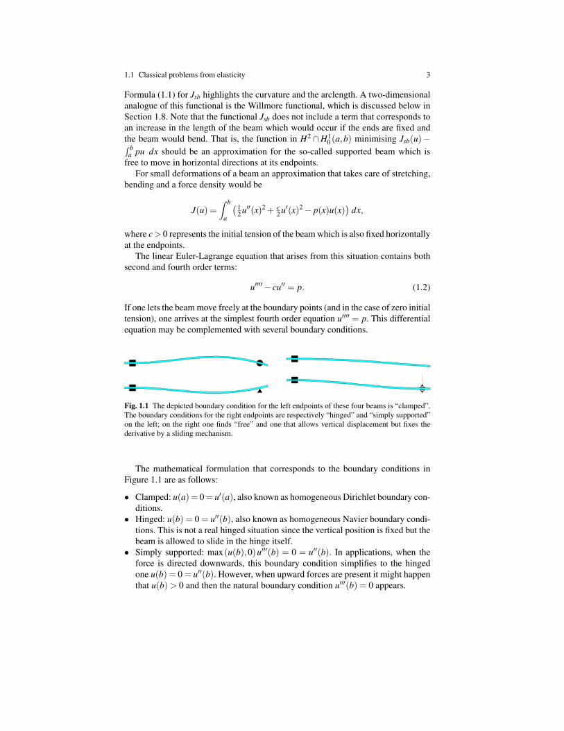
Fig. 1.1 The depicted boundary condition for the left endpoints of these four beams is “clamped”.The boundary conditions for the right endpoints are respectively “hinged” and “simply supported”on the left; on the right one finds “free” and one that allows vertical displacement but fixes thederivative by a sliding mechanism.
The mathematical formulation that corresponds to the boundary conditions inFigure 1.1 are as follows:
• Clamped: u(a) = 0 = u′(a), also known as homogeneous Dirichlet boundary con-ditions.
• Hinged: u(b) = 0 = u′′(b), also known as homogeneous Navier boundary condi-tions. This is not a real hinged situation since the vertical position is fixed but thebeam is allowed to slide in the hinge itself.
• Simply supported: max(u(b),0)u′′′(b) = 0 = u′′(b). In applications, when theforce is directed downwards, this boundary condition simplifies to the hingedone u(b) = 0 = u′′(b). However, when upward forces are present it might happenthat u(b) > 0 and then the natural boundary condition u′′′(b) = 0 appears.
4 1 Models of higher order
• Free: u′′′(b) = 0 = u′′(b).• Free vertical sliding but with fixed derivative: u′(b) = u′′′(b) = 0.
The second and third order derivatives appear as natural boundary conditions bythe derivation of the strong Euler-Lagrange equations.
If the beam would be moving in an elastic medium, then, again for small devia-tions one adds a further term to J and finds
J(u) =∫ b
a
( 12 (u′′)2 + γ
2 u2− pu)
dx.
This leads to the Euler-Lagrange equation u′′′′+ γu = p.
Also a suspension bridge may be seen as a beam of given length L, with hingedends and whose downward deflection is measured by a function u(x, t) subject tothree forces. These forces can be summarised as the stays holding the bridge up asnonlinear springs with spring constant k, the constant weight per unit length of thebridge W pushing it down, and the external forcing term f (x, t). This leads to theequation
utt + γuxxxx =−ku+ +W + f (x, t),
u(0, t) = u(L, t) = uxx(0, t) = uxx(L, t) = 0,(1.3)
where γ is a physical constant depending on the beam, Young’s modulus, and thesecond moment of inertia. The model leading to (1.3) is taken from the survey papers[270, 295].
The famous collapse of the Tacoma Narrows Bridge, see [16, 61], was the con-sequence of a torsional oscillation. McKenna [295, p. 106] explains this fact as fol-lows.
A large vertical motion had built up, there was a small push in the torsional direction tobreak symmetry, the instability occurred, and small aerodynamic torsional periodic forceswere sufficient to maintain the large periodic torsional motions.
For this reason, a major role is played by travelling waves. If one neglects theeffect of external forces and normalises all the constants, then (1.3) becomes
utt +uxxxx =−u+ +1 . (1.4)
In order to find travelling waves, one seeks solutions of (1.4) for (x, t) ∈ R2 of thekind u(x, t) = 1 + y(x− ct) where c > 0 denotes the speed of propagation. Hence,the function y satisfies the fourth order ordinary differential equation
y′′′′+ c2y′′+(y+1)+−1 = 0 in R .
This is a nonlinear version of (1.2). We refer to the papers [270, 271, 295, 297, 298]and references therein for variants of these equations and for a number of resultsand open problems related to suspension bridges.
1.1 Classical problems from elasticity 5
1.1.2 The Kirchhoff-Love model for a thin plate
As for the beam we assume that the plate, the vertical projection of which is theplanar region Ω ⊂ R2, is free to move horizontally at the boundary. Then a simplemodel for the elastic energy is
J(u) =∫
Ω
(12 (∆u)2 +(1−σ)
(u2
xy−uxxuyy)− f u
)dxdy, (1.5)
where f is the external vertical load. Again u is the deflection of the plate in ver-tical direction and, as above for the beam, first order derivatives are left out whichindicates that the plate is free to move horizontally.
This modern variational formulation appears already in [173], while a discussionfor a boundary value problem for a thin elastic plate in a somehow old fashionednotation is made already by Kirchhoff [249]. See also the two papers of Birman[57, 58], the books by Mikhlin [303, §30], Destuynder-Salaun [141], Ciarlet [102],or the article [103] for the clamped case.
In (1.5) σ is the Poisson ratio, which is defined by σ = λ
2(λ+µ) with the so-calledLame constants λ ,µ that depend on the material. For physical reasons it holds thatµ > 0 and usually λ ≥ 0 so that 0 ≤ σ < 1
2 . Moreover, it always holds true thatσ > −1 although some exotic materials have a negative Poisson ratio, see [265].For metals the value σ lies around 0.3 (see [280, p. 105]). One should observe thatfor σ >−1, the quadratic part of the functional (1.5) is always positive.
For small deformations the terms in (1.5) are taken as approximations beingpurely quadratic with respect to the second derivatives of u of respectively twicethe squared mean curvature and the Gaussian curvature supplied with the factorσ −1. For those small deformations one finds
12 (∆u)2 +(1−σ)
(u2
xy−uxxuyy)≈ 1
2 (κ1 +κ2)2− (1−σ)κ1κ2
= 12 κ
21 +σκ1κ2 + 1
2 κ22 ,
where κ1, κ2 are the principal curvatures of the graph of u. Variational integralsavoiding such approximations and involving the original expressions for the meanand the Gaussian curvature are considered in Section 1.8 and lead as a special caseto the Willmore functional.
Which are the appropriate boundary conditions? For the clamped and hingedboundary condition the natural settings, that is the Hilbert spaces for these two sit-uations, are respectively H = H2
0 (Ω) and H = H2∩H10 (Ω). Minimising the energy
functional leads to the weak Euler-Lagrange equation 〈dJ(u),v〉= 0, that is∫Ω
(∆u∆v+(1−σ)(2uxyvxy−uxxvyy−uyyvxx)− f v) dxdy = 0 (1.6)
for all v∈H. Let us assume both that minimisers u lie in H4(Ω) and that the exteriornormal ν = (ν1,ν2) and the corresponding tangential τ = (τ1,τ2) = (−ν2,ν1) arewell-defined. Then an integration by parts of (1.6) leads to
6 1 Models of higher order
0 =∫
Ω
(∆
2u− f)
v dxdy +∫
∂Ω
(∂
∂ν∆u)
v ds
+ (1−σ)∫
∂Ω
((ν
21 −ν
22)
uxy−ν1ν2 (uxx−uyy))
∂
∂τv ds
+∫
∂Ω
(∆u+(1−σ)
(2ν1ν2uxy−ν
22 uxx−ν
21 uyy
)) ∂
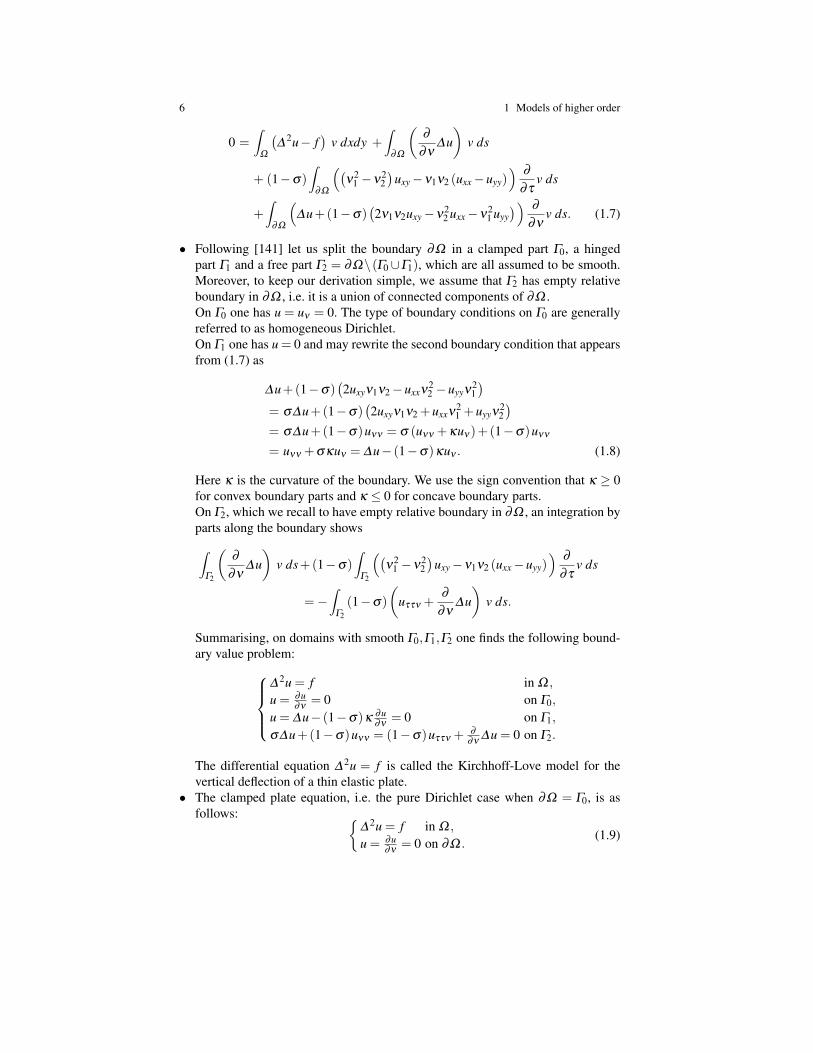
∂νv ds. (1.7)
• Following [141] let us split the boundary ∂Ω in a clamped part Γ0, a hingedpart Γ1 and a free part Γ2 = ∂Ω\(Γ0∪Γ1), which are all assumed to be smooth.Moreover, to keep our derivation simple, we assume that Γ2 has empty relativeboundary in ∂Ω , i.e. it is a union of connected components of ∂Ω .On Γ0 one has u = uν = 0. The type of boundary conditions on Γ0 are generallyreferred to as homogeneous Dirichlet.On Γ1 one has u = 0 and may rewrite the second boundary condition that appearsfrom (1.7) as
∆u+(1−σ)(2uxyν1ν2−uxxν
22 −uyyν
21)
= σ∆u+(1−σ)(2uxyν1ν2 +uxxν
21 +uyyν
22)
= σ∆u+(1−σ)uνν = σ (uνν +κuν)+(1−σ)uνν
= uνν +σκuν = ∆u− (1−σ)κuν . (1.8)
Here κ is the curvature of the boundary. We use the sign convention that κ ≥ 0for convex boundary parts and κ ≤ 0 for concave boundary parts.On Γ2, which we recall to have empty relative boundary in ∂Ω , an integration byparts along the boundary shows∫
Γ2
(∂
∂ν∆u)
v ds+(1−σ)∫
Γ2
((ν
21 −ν
22)
uxy−ν1ν2 (uxx−uyy))
∂
∂τv ds
=−∫
Γ2
(1−σ)(
uττν +∂
∂ν∆u)
v ds.
Summarising, on domains with smooth Γ0,Γ1,Γ2 one finds the following bound-ary value problem:
∆ 2u = f in Ω ,
u = ∂u∂ν
= 0 on Γ0,
u = ∆u− (1−σ)κ∂u∂ν
= 0 on Γ1,
σ∆u+(1−σ)uνν = (1−σ)uττν + ∂
∂ν∆u = 0 on Γ2.
The differential equation ∆ 2u = f is called the Kirchhoff-Love model for thevertical deflection of a thin elastic plate.
• The clamped plate equation, i.e. the pure Dirichlet case when ∂Ω = Γ0, is asfollows:
∆ 2u = f in Ω ,
u = ∂u∂ν
= 0 on ∂Ω .(1.9)
1.1 Classical problems from elasticity 7
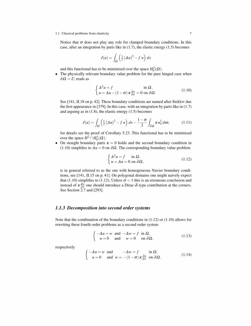
Notice that σ does not play any role for clamped boundary conditions. In thiscase, after an integration by parts like in (1.7), the elastic energy (1.5) becomes
J(u) =∫
Ω
(12 (∆u)2− f u
)dx
and this functional has to be minimised over the space H20 (Ω).
• The physically relevant boundary value problem for the pure hinged case when∂Ω = Γ1 reads as
∆ 2u = f in Ω ,
u = ∆u− (1−σ)κ∂u∂ν
= 0 on ∂Ω .(1.10)
See [141, II.18 on p. 42]. These boundary conditions are named after Steklov duethe first appearance in [379]. In this case, with an integration by parts like in (1.7)and arguing as in (1.8), the elastic energy (1.5) becomes
J(u) =∫
Ω
(12 (∆u)2− f u
)dx− 1−σ
2
∫∂Ω
κ u2ν dω; (1.11)
for details see the proof of Corollary 5.23. This functional has to be minimisedover the space H2∩H1
0 (Ω).• On straight boundary parts κ = 0 holds and the second boundary condition in
(1.10) simplifies to ∆u = 0 on ∂Ω . The corresponding boundary value problem∆ 2u = f in Ω ,u = ∆u = 0 on ∂Ω ,
(1.12)
is in general referred to as the one with homogeneous Navier boundary condi-tions, see [141, II.15 on p. 41]. On polygonal domains one might naively expectthat (1.10) simplifies to (1.12). Unless σ = 1 this is an erroneous conclusion andinstead of κ
∂u∂ν
one should introduce a Dirac-δ -type contribution at the corners.See Section 2.7 and [293].
1.1.3 Decomposition into second order systems
Note that the combination of the boundary conditions in (1.12) or (1.10) allows forrewriting these fourth order problems as a second order system
−∆u = w and −∆w = f in Ω ,u = 0 and w = 0 on ∂Ω ,
(1.13)
respectively −∆u = w and −∆w = f in Ω ,
u = 0 and w =−(1−σ)κ∂u∂ν
on ∂Ω .(1.14)
8 1 Models of higher order
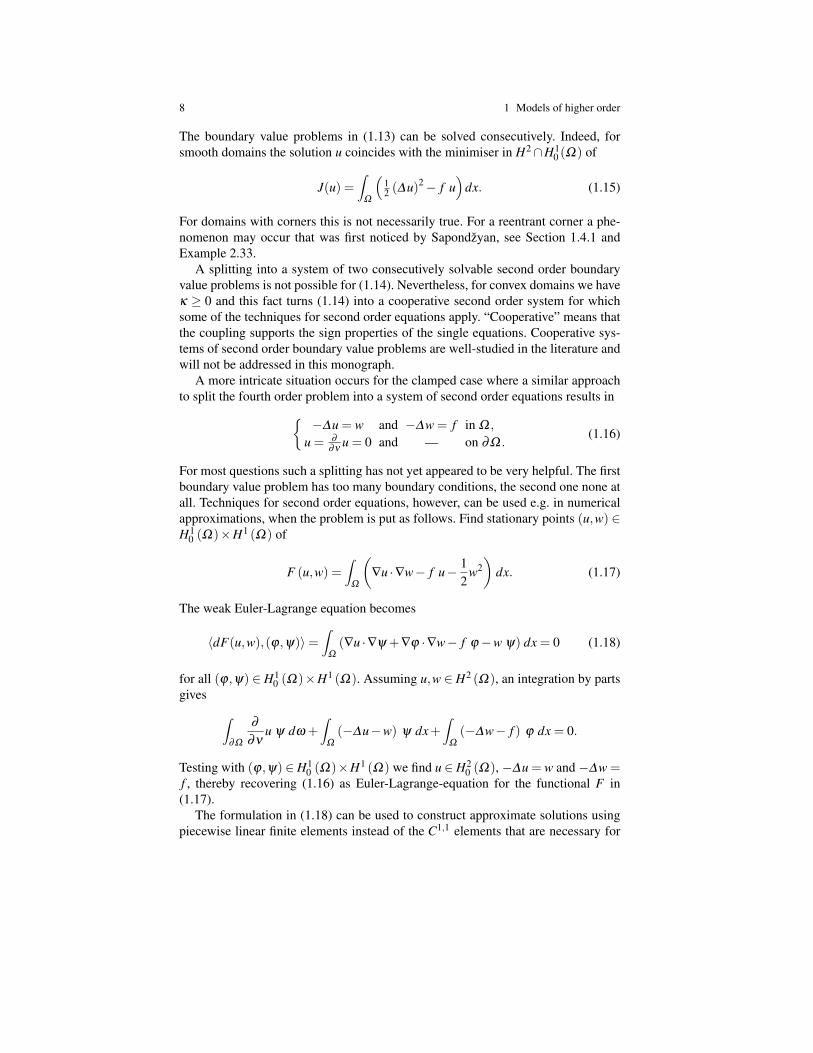
The boundary value problems in (1.13) can be solved consecutively. Indeed, forsmooth domains the solution u coincides with the minimiser in H2∩H1
0 (Ω) of
J(u) =∫
Ω
(12 (∆u)2− f u
)dx. (1.15)
For domains with corners this is not necessarily true. For a reentrant corner a phe-nomenon may occur that was first noticed by Sapondzyan, see Section 1.4.1 andExample 2.33.
A splitting into a system of two consecutively solvable second order boundaryvalue problems is not possible for (1.14). Nevertheless, for convex domains we haveκ ≥ 0 and this fact turns (1.14) into a cooperative second order system for whichsome of the techniques for second order equations apply. “Cooperative” means thatthe coupling supports the sign properties of the single equations. Cooperative sys-tems of second order boundary value problems are well-studied in the literature andwill not be addressed in this monograph.
A more intricate situation occurs for the clamped case where a similar approachto split the fourth order problem into a system of second order equations results in
−∆u = w and −∆w = f in Ω ,
u = ∂
∂νu = 0 and — on ∂Ω .
(1.16)
For most questions such a splitting has not yet appeared to be very helpful. The firstboundary value problem has too many boundary conditions, the second one none atall. Techniques for second order equations, however, can be used e.g. in numericalapproximations, when the problem is put as follows. Find stationary points (u,w) ∈H1
0 (Ω)×H1 (Ω) of
F (u,w) =∫
Ω
(∇u ·∇w− f u− 1
2w2)
dx. (1.17)
The weak Euler-Lagrange equation becomes
〈dF(u,w),(ϕ,ψ)〉=∫
Ω
(∇u ·∇ψ +∇ϕ ·∇w− f ϕ−w ψ) dx = 0 (1.18)
for all (ϕ,ψ) ∈ H10 (Ω)×H1 (Ω). Assuming u,w ∈ H2 (Ω), an integration by parts
gives ∫∂Ω
∂
∂νu ψ dω +
∫Ω
(−∆u−w) ψ dx+∫
Ω
(−∆w− f ) ϕ dx = 0.
Testing with (ϕ,ψ) ∈H10 (Ω)×H1 (Ω) we find u ∈H2
0 (Ω), −∆u = w and −∆w =f , thereby recovering (1.16) as Euler-Lagrange-equation for the functional F in(1.17).
The formulation in (1.18) can be used to construct approximate solutions usingpiecewise linear finite elements instead of the C1,1 elements that are necessary for
1.2 The Boggio-Hadamard conjecture for a clamped plate 9
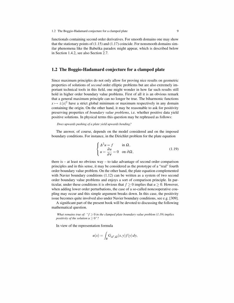
functionals containing second order derivatives. For smooth domains one may showthat the stationary points of (1.15) and (1.17) coincide. For nonsmooth domains sim-ilar phenomena like the Babuska paradox might appear, which is described belowin Section 1.4.2, see also Section 2.7.
1.2 The Boggio-Hadamard conjecture for a clamped plate
Since maximum principles do not only allow for proving nice results on geometricproperties of solutions of second order elliptic problems but are also extremely im-portant technical tools in this field, one might wonder in how far such results stillhold in higher order boundary value problems. First of all it is an obvious remarkthat a general maximum principle can no longer be true. The biharmonic functionsx 7→ ±|x|2 have a strict global minimum or maximum respectively in any domaincontaining the origin. On the other hand, it may be reasonable to ask for positivitypreserving properties of boundary value problems, i.e. whether positive data yieldpositive solutions. In physical terms this question may be rephrased as follows:
Does upwards pushing of a plate yield upwards bending?
The answer, of course, depends on the model considered and on the imposedboundary conditions. For instance, in the Dirichlet problem for the plate equation∆
2u = f in Ω ,
u =∂u∂ν
= 0 on ∂Ω ,(1.19)
there is – at least no obvious way – to take advantage of second order comparisonprinciples and in this sense, it may be considered as the prototype of a “real” fourthorder boundary value problem. On the other hand, the plate equation complementedwith Navier boundary conditions (1.12) can be written as a system of two secondorder boundary value problems and enjoys a sort of comparison principle. In par-ticular, under these conditions it is obvious that f ≥ 0 implies that u≥ 0. However,when adding lower order perturbations, the case of a so-called noncooperative cou-pling may occur and this simple argument breaks down. In this case, the positivityissue becomes quite involved also under Navier boundary conditions, see e.g. [309].
A significant part of the present book will be devoted to discussing the followingmathematical question.
What remains true of: “ f ≥ 0 in the clamped plate boundary value problem (1.19) impliespositivity of the solution u≥ 0”?
In view of the representation formula
u(x) =∫
BG∆ 2,Ω (x,y) f (y)dy,
10 1 Models of higher order
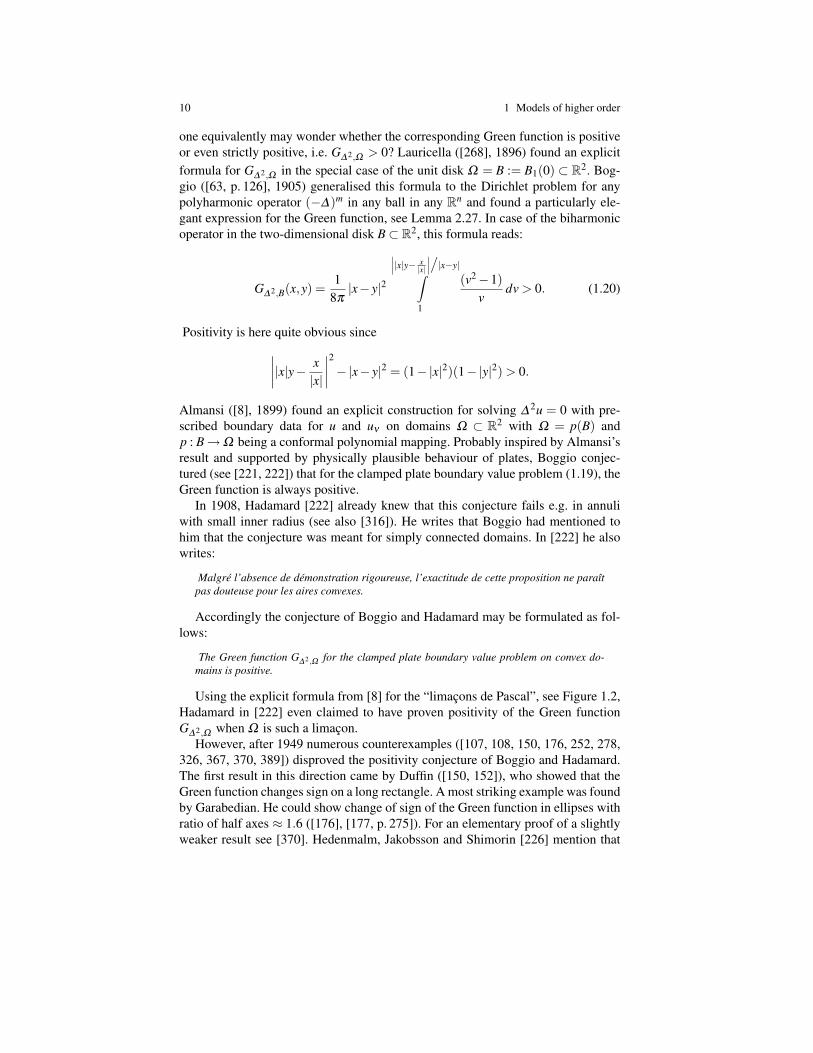
one equivalently may wonder whether the corresponding Green function is positiveor even strictly positive, i.e. G∆ 2,Ω > 0? Lauricella ([268], 1896) found an explicitformula for G∆ 2,Ω in the special case of the unit disk Ω = B := B1(0) ⊂ R2. Bog-gio ([63, p. 126], 1905) generalised this formula to the Dirichlet problem for anypolyharmonic operator (−∆)m in any ball in any Rn and found a particularly ele-gant expression for the Green function, see Lemma 2.27. In case of the biharmonicoperator in the two-dimensional disk B⊂ R2, this formula reads:
G∆ 2,B(x,y) =1
8π|x− y|2
∣∣∣|x|y− x|x|
∣∣∣/|x−y|∫1
(v2−1)v
dv > 0. (1.20)
Positivity is here quite obvious since∣∣∣∣|x|y− x|x|
∣∣∣∣2−|x− y|2 = (1−|x|2)(1−|y|2) > 0.
Almansi ([8], 1899) found an explicit construction for solving ∆ 2u = 0 with pre-scribed boundary data for u and uν on domains Ω ⊂ R2 with Ω = p(B) andp : B→Ω being a conformal polynomial mapping. Probably inspired by Almansi’sresult and supported by physically plausible behaviour of plates, Boggio conjec-tured (see [221, 222]) that for the clamped plate boundary value problem (1.19), theGreen function is always positive.
In 1908, Hadamard [222] already knew that this conjecture fails e.g. in annuliwith small inner radius (see also [316]). He writes that Boggio had mentioned tohim that the conjecture was meant for simply connected domains. In [222] he alsowrites:
Malgre l’absence de demonstration rigoureuse, l’exactitude de cette proposition ne paraıtpas douteuse pour les aires convexes.
Accordingly the conjecture of Boggio and Hadamard may be formulated as fol-lows:
The Green function G∆ 2,Ω for the clamped plate boundary value problem on convex do-mains is positive.
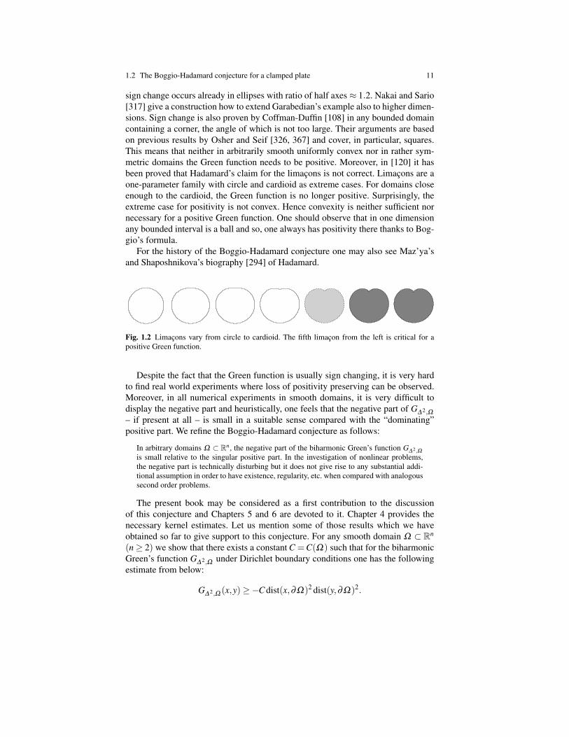
Using the explicit formula from [8] for the “limacons de Pascal”, see Figure 1.2,Hadamard in [222] even claimed to have proven positivity of the Green functionG∆ 2,Ω when Ω is such a limacon.
However, after 1949 numerous counterexamples ([107, 108, 150, 176, 252, 278,326, 367, 370, 389]) disproved the positivity conjecture of Boggio and Hadamard.The first result in this direction came by Duffin ([150, 152]), who showed that theGreen function changes sign on a long rectangle. A most striking example was foundby Garabedian. He could show change of sign of the Green function in ellipses withratio of half axes ≈ 1.6 ([176], [177, p. 275]). For an elementary proof of a slightlyweaker result see [370]. Hedenmalm, Jakobsson and Shimorin [226] mention that
1.2 The Boggio-Hadamard conjecture for a clamped plate 11
sign change occurs already in ellipses with ratio of half axes≈ 1.2. Nakai and Sario[317] give a construction how to extend Garabedian’s example also to higher dimen-sions. Sign change is also proven by Coffman-Duffin [108] in any bounded domaincontaining a corner, the angle of which is not too large. Their arguments are basedon previous results by Osher and Seif [326, 367] and cover, in particular, squares.This means that neither in arbitrarily smooth uniformly convex nor in rather sym-metric domains the Green function needs to be positive. Moreover, in [120] it hasbeen proved that Hadamard’s claim for the limacons is not correct. Limacons are aone-parameter family with circle and cardioid as extreme cases. For domains closeenough to the cardioid, the Green function is no longer positive. Surprisingly, theextreme case for positivity is not convex. Hence convexity is neither sufficient nornecessary for a positive Green function. One should observe that in one dimensionany bounded interval is a ball and so, one always has positivity there thanks to Bog-gio’s formula.
For the history of the Boggio-Hadamard conjecture one may also see Maz’ya’sand Shaposhnikova’s biography [294] of Hadamard.
Fig. 1.2 Limacons vary from circle to cardioid. The fifth limacon from the left is critical for apositive Green function.
Despite the fact that the Green function is usually sign changing, it is very hardto find real world experiments where loss of positivity preserving can be observed.Moreover, in all numerical experiments in smooth domains, it is very difficult todisplay the negative part and heuristically, one feels that the negative part of G∆ 2,Ω
– if present at all – is small in a suitable sense compared with the “dominating”positive part. We refine the Boggio-Hadamard conjecture as follows:
In arbitrary domains Ω ⊂ Rn, the negative part of the biharmonic Green’s function G∆ 2,Ωis small relative to the singular positive part. In the investigation of nonlinear problems,the negative part is technically disturbing but it does not give rise to any substantial addi-tional assumption in order to have existence, regularity, etc. when compared with analogoussecond order problems.
The present book may be considered as a first contribution to the discussionof this conjecture and Chapters 5 and 6 are devoted to it. Chapter 4 provides thenecessary kernel estimates. Let us mention some of those results which we haveobtained so far to give support to this conjecture. For any smooth domain Ω ⊂ Rn
(n≥ 2) we show that there exists a constant C = C(Ω) such that for the biharmonicGreen’s function G∆ 2,Ω under Dirichlet boundary conditions one has the followingestimate from below:
G∆ 2,Ω (x,y)≥−C dist(x,∂Ω)2 dist(y,∂Ω)2.
12 1 Models of higher order
This means that although in general, G∆ 2,Ω has a nontrivial negative part, this be-haves completely regular and is in this respect not affected by the singularity of theGreen’s function. Qualitatively, only its positive part is affected by its singularity.See Theorem 6.24 and the subsequent remarks. Moreover, in Theorems 6.3 and 6.29we show that positivity in the Dirichlet problem for the biharmonic operator doeshold true not only in balls but also in smooth domains which are close to balls ina suitably strong sense. Although being a perturbation result it is not just a conse-quence of continuous dependence on data. The problem in proving positivity forGreen’s functions consists in gaining uniformity when their singularities approachthe boundaries.
Finally, in Section 5.4 positivity issues for the biharmonic operator under Steklovboundary conditions are addressed. With respect to positivity it may be considered,at least in some cases, to be intermediate between Dirichlet conditions on the onehand and Navier boundary conditions on the other hand, see Theorems 5.26 and5.27.
1.3 The first eigenvalue
It is well-known that for general second order elliptic Dirichlet problems the eigen-function ϕ1 that corresponds to the first eigenvalue is of one sign. In case of theLaplacian such a result can be proven directly sticking to the variational characteri-sation of the first eigenvalue
Λ1,1 := minv∈H1
0 \0
∫|∇v|2 dx∫|v|2 dx
=∫|∇ϕ1|2 dx∫|ϕ1|2 dx
by comparing |ϕ1| with ϕ1. For quite general and even non-selfadjoint second orderDirichlet problems the same result is proven by using more abstract results such asthe Kreın-Rutman theorem. The first approach uses the truncation method and so,a version of the maximum principle, while the Kreın-Rutman theorem requires thepresence of a comparison principle. A simple alternative is provided by the dualcone method of Moreau [311]. This approach, which is explained in Section 3.1.2,is on one hand restricted to a symmetric setting in a Hilbert space but on the otherhand, can also be applied in semilinear problems.
Considering Ω 7→ Λ1,1(Ω) in dependence of the domains Ω being subject tohaving all the same volume as the unit ball B ⊂ Rn one may wonder whether thismap is minimised for Ω = B. Indeed, this was proved by Faber-Krahn [162, 253,254] and, moreover, balls of radius 1 are the only minimisers.
1.3 The first eigenvalue 13
1.3.1 The Dirichlet eigenvalue problem
Whenever the biharmonic operator under Dirichlet boundary conditions has astrictly positive Green’s function, the first eigenvalue Λ2,1 is simple and the cor-responding first eigenfunction is of fixed sign, see Section 3.1.3. Related to the firsteigenvalue is a question posed by Lord Rayleigh in 1894 in his celebrated mono-graph [350]. He studied the vibration of (planar) plates and conjectured that amongdomains of given area, when the edges are clamped, the form of gravest pitch isdoubtless the circle, see [350, p. 382]. This corresponds to saying that
Λ2,1(B)≤Λ2,1(Ω) whenever |Ω |= π (1.21)
for planar domains (n = 2). Szego [388] assumed that in any domain the first eigen-function for the clamped plate has always a fixed sign and proved that this hypoth-esis would imply the isoperimetric inequality (1.21). The assumption that the firsteigenfunction is of fixed sign, however, is not true as Duffin pointed out. In [152],where he explains some counterexamples, he referred to this assumption as Szego’sconjecture on the clamped plate. Details of these counterexamples can be found in[153, 154, 155].
Subsequently, concerning Rayleigh’s conjecture, Mohr [310] showed in 1975that if among all domains of given area there exists a smooth minimiser for Λ2,1then the domain is a disk. However, he left open the question of existence. In 1981,Talenti [392] extended Szego’s result in two directions. He showed that the state-ment remains true under the weaker assumption that the nodal set of the first eigen-function ϕ1 of (3.1) is empty or is included in x ∈Ω ; ∇ϕ1 = 0. This result holdsin any space dimension n ≥ 2. Moreover, for general domains, instead of (1.21) heshowed that
CnΛ2,1(B)≤Λ2,1(Ω) whenever |Ω |= en
where 0.5 < Cn < 1 is a constant depending on the dimension n. These constantswere increased by Ashbaugh-Laugesen [24] who also showed that Cn → 1 as n→∞.
A complete proof of Rayleigh’s conjecture was finally obtained one century laterthan the conjecture itself in a celebrated paper by Nadirashvili [315]. This result wasimmediately extended by Ashbaugh-Benguria [22] to the case of domains in R3.
More results about the positivity of the first eigenfunction in general domainsand a proof of Rayleigh’s conjecture can be found in Chapter 3.
1.3.2 An eigenvalue problem for a buckled plate
In 1910, Th. von Karman [403] described the large deflections and stresses producedin a thin elastic plate subject to compressive forces along its edge by means of a sys-tem of two fourth order elliptic quasilinear equations. For a derivation of this modelfrom three dimensional elasticity one may also see [174] and references therein. An

14 1 Models of higher order
interesting phenomenon associated with this nonlinear model is the appearance of“buckling”, namely the plate may deflect out of its plane when these forces reach acertain magnitude. We also refer to more recent work in [48, 101].
The linearisation of the von Karman equations for an elastic plate over planardomains Ω ⊂ R2 under pressure leads to the following eigenvalue problem
∆ 2u =−µ∆u in Ω ,u = ∆u− (1−σ)κuν = 0 on ∂Ω .
(1.22)
Miersemann [301] studied this eigenvalue problem and he was one of the first to ap-ply the dual cone setting of Moreau [311] to a fourth order boundary value problem.He could show that on convex C2,γ -domains the first eigenvalue for (1.22) is simpleand that the corresponding eigenfunction is of fixed sign. The setting introduced byMoreau will be also most convenient for a number of nonlinear problems as we shalloutline in Chapters 3 and 7, see in particular Sections 7.2.3 and 7.3.
We also consider the Dirichlet eigenvalue problem∆ 2u =−µ∆u in Ω ,u = uν = 0 on ∂Ω ,
(1.23)
related to (1.22) and where the least eigenvalue µ1(Ω) represents the buckling loadof a clamped plate. Inspired by Rayleigh’s conjecture (1.21), Polya-Szego [343,Note F] conjectured that
µ1(B)≤ µ1(Ω) whenever |Ω |= π (1.24)
for any bounded planar domain Ω ⊂R2. And again, using rearrangement techniquesthey proved (1.24) under the assumption that the solution u to (1.23) is positive, see[343, 388]. Unfortunately, as for the clamped plate eigenvalue, this property failsin general, for instance in the square (0,1)2, see Wieners [412]. Without imposingthis sign assumption on the first eigenfunction, Ashbaugh-Laugesen [24] proved thebound γµ1(B)≤ µ1(Ω) whenever |Ω |= π for γ = 0.78 . . . which is, of course, muchweaker than (1.24).
A complete proof of (1.24) is not yet known. A quite well established strategywhich could be used to prove (1.24) involves shape derivatives, see e.g. [228]. Itmainly consists in three steps.
1. In a suitable class of domains, prove the existence of a minimiser Ωo for the mapΩ 7→ µ1(Ω).
2. Prove that ∂Ωo is smooth, for instance ∂Ωo ∈C2,γ , in order to be able to computethe derivative of Ω 7→ µ1(Ω) and to impose that it vanishes when Ω = Ωo.
3. Exploit the just obtained stationarity condition, which usually gives an overde-termined condition on ∂Ωo, to prove that Ωo is a ball.
In Section 3.2 we show how Item 1 has been successfully settled by Ashbaugh-Bucur [23] and how Item 3 has been achieved by Weinberger-Willms [415], see
1.3 The first eigenvalue 15
also [244, Proposition 4.4]. Therefore, for a complete proof of (1.24), “only” Item2 is missing!
1.3.3 A Steklov eigenvalue problem
Usually, eigenvalue problems arise when one studies oscillation modes in the re-spective time dependent problem in order to have a physically well motivated theoryand representation of solutions.
However, in what follows, a most natural motivation for considering a furthereigenvalue problem comes from a seemingly quite different mathematical question.We explain how L2-estimates for the Dirichlet problem for harmonic functions linkwith the Steklov eigenvalue problem for biharmonic functions.
Let Ω ⊂ Rn be a bounded smooth domain and consider the problem∆u = 0 in Ω ,u = g on ∂Ω ,
(1.25)
where g ∈ L2(∂Ω). It is well-known that (1.25) admits a unique solution u ∈H1/2(Ω) ⊂ L2(Ω), see e.g. [275, Remarque 7.2, p. 202] and also [237, 238] foran extension to nonsmooth domains. One is then interested in a priori estimates,namely in determining the sharp constant CΩ such that
‖u‖L2(Ω) ≤CΩ‖g‖L2(∂Ω).
By Fichera’s principle of duality [170] (see also Section 3.3.2) one sees that CΩ
coincides with the inverse of the first Steklov eigenvalue δ1 = δ1(Ω), namely thesmallest constant a such that the problem
∆ 2u = 0 in Ω ,u = ∆u−auν = 0 on ∂Ω ,
(1.26)
admits a nontrivial solution. Notice that the “true” eigenvalue problem for the hingedplate equation should include the curvature in the second boundary condition, see(1.8). The map Ω 7→ δ1(Ω) has several surprising properties which we establishin Section 3.3.2. By rescaling, one sees that δ1(kΩ) = k−1δ1(Ω) for any boundeddomain Ω and any k > 0 so that δ1(kΩ) → 0 as k → ∞. One is then led to seekdomains which minimise δ1 under suitable constraints, the most natural one beingthe volume constraint. Smith [373] stated that, analogously to the Faber-Krahn result[162, 253, 254], the minimiser for δ1 should exist and be a ball, at least for planardomains. But, as noticed by Kuttler and Sigillito, the argument in [373] contains agap. In the “Note added in proof” in [374, p. 111], Smith writes:
Although the result is probably true, a correct proof has not yet been found.
16 1 Models of higher order
A few years later, Kuttler [258] proved that a (planar) square has a first Stekloveigenvalue δ1(Ω) which is strictly smaller than the one of the disk having the samemeasure. The estimate by Kuttler was subsequently improved in [165]. Therefore,it is not true that δ1(Ω ∗) ≤ δ1(Ω) where Ω ∗ denotes the spherical rearrangementof Ω . For this reason, Kuttler [258] suggested a different minimisation problemwith a perimeter constraint; in [258, Formula (11)] he conjectures that a planar diskminimises δ1 among all domains having fixed perimeter. He provides numerical ev-idence that on rectangles his conjecture seems true, see also [259, 261]. In Theorem3.24 we show that also this conjecture is false and that an optimal shape for δ1 doesnot exist under a perimeter constraint in any space dimension n ≥ 2. In fact, undersuch a constraint, the infimum of δ1 is zero.
The spectrum of (1.26) has a nice application in functional analysis. In Section3.3.1 we show that the closure of the space spanned by the Steklov eigenfunctionsis the orthogonal complement of H2
0 (Ω) in H2∩H10 (Ω).
1.4 Paradoxes for the hinged plate
The most common domains for plate problems that appear in engineering are poly-gonal ones. On the straight boundary parts of a polygonal domain the hinged bound-ary conditions (1.10) lead to Navier boundary conditions (1.12). Without taking careof a possible singularity due to “κ = ∞” in the corners it would mean that the so-lution no longer depends on the Poisson ratio σ . Sapondzyan [357] noticed thatthe solution one obtains by solving (1.12) iteratively does not necessarily have abounded energy. Babuska noticed in [28] that the difference between (1.10) and(1.12) would mean that by approximating a curvilinear domain by polygons, as isdone in most finite elements methods, the approximating solutions would not con-verge to the solution on the curvilinear domain.
Although both paradoxes are usually referred to by the name Babuska, they docover different phenomena as we will explain in more detail.
1.4.1 Sapondzyan’s paradox by concave corners
One might expect that the problem that appeared in these paradoxes is due to aboundary condition not being well-defined in corners. Indeed, the curvature thatappears in the boundary condition is singular and apparently leads to a δ -distributiontype contribution. By adding appropriate extra terms in the corners there is somehope to find the real solution. The situation for reentrant corners can be ‘worse’.Due to Kondratiev [65, 251], Maz’ya et al. [288, 289], Grisvard [199] and manyothers, it is well-known that corners may lead to a loss of regularity. It is less knownthat a corner may lead to multiple solutions, that is, the solution depends cruciallyon the space that one chooses.
1.4 Paradoxes for the hinged plate 17
An example where two different solutions appear naturally from two straightfor-ward settings goes as follows. Both fourth order boundary value problems, hinged orSteklov (1.10) as well as Navier (1.12) boundary conditions, allow a reformulationas a coupled system, see (1.14) and (1.13), respectively. In the latter case, one tendsto solve by an iteration of the Green operator for the second order Poisson problem.This approach works fine for bounded smooth domains, but whenever the domainhas a nonconvex corner, one does not necessarily get the solution one is looking for.Indeed, for the fourth order problem the natural setting for a weak solution to theNavier boundary value problem would be H2∩H1
0 (Ω). The second Navier bound-ary condition ∆u = 0 would follow naturally on smooth boundary parts from theweak formulation where u satisfies∫
Ω
(∆u∆ϕ− f ϕ) dx = 0 for all ϕ ∈ H2∩H10 (Ω). (1.27)
However, for the system in (1.13) the natural setting is that one looks for functionpairs (u,v)∈H1
0 (Ω)×H10 (Ω). In [320] it is shown that for domains with a reentrant
corner both problems have a unique solution but the solutions u1 to (1.13) and u2to (1.27) are different. Indeed, there exist a constant c f and a nontrivial biharmonicfunction b that satisfies (1.13) with zero Navier boundary condition except in thecorner such that u1 = u2 + c f b. The related problem for domains with edges is con-sidered in [319]. We refer to Section 2.7 for more details and an explicit example.
1.4.2 The Babuska paradox
In the original Babuska or polygon-circle paradox one considers problem (1.10) forf = 1 and when Ω = Pm ⊂ B (m ≥ 3) is the interior of the regular polygon withcorners e2kπi/m for k ∈ N, namely
∆ 2u = 1 in Pm,
u = ∆u = 0 on ∂Pm.
If um denotes the solution of this problem extended by 0 in B\Pm, it can be shownthat the sequence (um) converges uniformly to
u∞(x) :=364− 1
16|x|2 +
164|x|4
which is not the solution to the “limit problem” (where κ = 1), namely∆ 2u = 1 in B,
u = ∆u− (1−σ)κ∂u∂ν
= 0 on ∂B
unless σ = 1, see Figure 1.3.For more details on this Babuska paradox see Section 2.7.
18 1 Models of higher order
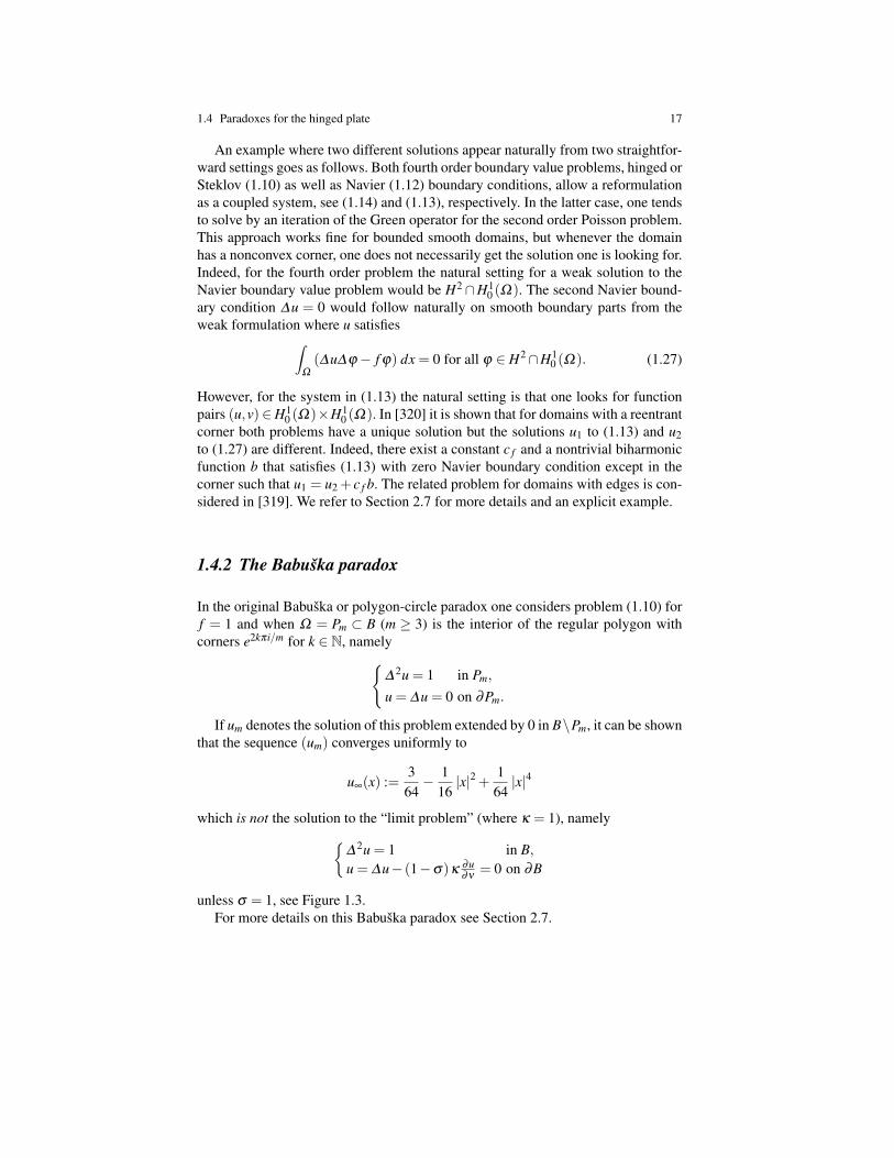
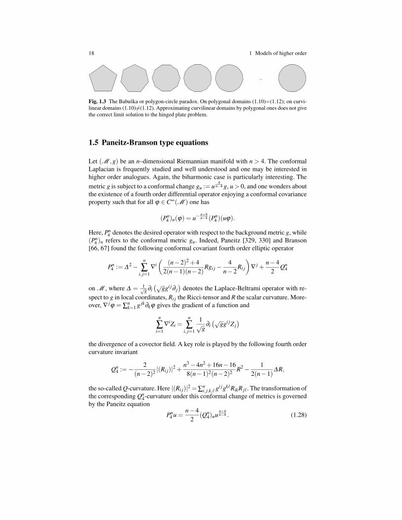
...
Fig. 1.3 The Babuska or polygon-circle paradox. On polygonal domains (1.10)=(1.12); on curvi-linear domains (1.10)6=(1.12). Approximating curvilinear domains by polygonal ones does not givethe correct limit solution to the hinged plate problem.
1.5 Paneitz-Branson type equations
Let (M ,g) be an n–dimensional Riemannian manifold with n > 4. The conformalLaplacian is frequently studied and well understood and one may be interested inhigher order analogues. Again, the biharmonic case is particularly interesting. Themetric g is subject to a conformal change gu := u
4n−4 g, u > 0, and one wonders about
the existence of a fourth order differential operator enjoying a conformal covarianceproperty such that for all ϕ ∈C∞(M ) one has
(Pn4 )u(ϕ) = u−
n+4n−4 (Pn
4 )(uϕ).
Here, Pn4 denotes the desired operator with respect to the background metric g, while
(Pn4 )u refers to the conformal metric gu. Indeed, Paneitz [329, 330] and Branson
[66, 67] found the following conformal covariant fourth order elliptic operator
Pn4 := ∆
2−n
∑i, j=1
∇i(
(n−2)2 +42(n−1)(n−2)
Rgi j−4
n−2Ri j
)∇
j +n−4
2Qn
4
on M , where ∆ = 1√g ∂i(√
ggi j∂ j)
denotes the Laplace-Beltrami operator with re-spect to g in local coordinates, Ri j the Ricci-tensor and R the scalar curvature. More-over, ∇ jϕ = ∑
nk=1 g jk∂kϕ gives the gradient of a function and
n
∑i=1
∇iZi =
n
∑i, j=1
1√
g∂i(√
ggi jZ j)
the divergence of a covector field. A key role is played by the following fourth ordercurvature invariant
Qn4 :=− 2
(n−2)2 |(Ri j)|2 +n3−4n2 +16n−16
8(n−1)2(n−2)2 R2− 12(n−1)
∆R,
the so-called Q-curvature. Here |(Ri j)|2 = ∑ni, j,k,` gi jgk`RikR j`. The transformation of
the corresponding Qn4-curvature under this conformal change of metrics is governed
by the Paneitz equation
Pn4 u =
n−42
(Qn4)uu
n+4n−4 . (1.28)
1.5 Paneitz-Branson type equations 19
In analogy to the second order Yamabe problem (for an overview see [381, SectionIII.4]), obvious questions here concern the existence of conformal metrics with con-stant or prescribed Q-curvature. Huge work has so far been done by research groupsaround Chang-Yang-Gursky and Hebey, as well as many others. For a survey andreferences see the books by Chang [89] and by Druet-Hebey-Robert [149]. Diffi-cult problems arise from ensuring the positivity requirement of the conformal factoru > 0 and from the necessity to know about the kernel of the Paneitz operator. Theseproblems have only been solved partly yet.
In order to explain the geometrical importance of the Q-curvature, we assumenow for a moment that the manifold (M ,g) is four-dimensional. Then, the Paneitzoperator is defined by
P44 := ∆
2−4
∑i, j=1
∇i(
23
Rgi j−2Ri j
)∇
j
in such a way that under the conformal change of metrics gu = e2ug one has
(P44 )u(ϕ) = e−4uP4
4 (ϕ).
In order to achieve a prescribed Q-curvature on the four-dimensional manifold(M ,gu), one has to find u solving
P44 u+2Q4
4 = 2Qe4u,
where Q44 is the curvature invariant
12Q44 =−∆R+R2−3|(Ri j)|2.
In this situation, one has the following Gauss-Bonnet-formula∫M
(Q+
18|W |2
)dS = 4π
2χ(M ),
where W is the Weyl tensor and χ(M ) is the Euler characteristic. Since χ(M ) is atopological and |W |2dS is a pointwise conformal invariant, this shows that
∫M QdS
is a conformal invariant, which governs e.g. the existence of conformal Ricci pos-itive metrics (see e.g. Chang-Gursky-Yang [90, 91]) and eigenvalue estimates forDirac operators (see Guofang Wang [407]). All these facts show that the Q-curvaturein the context of fourth order conformally covariant operators takes a role quite anal-ogous to the scalar curvature with respect to second order operators.
Getting back to the general case n > 4, let us outline what we are going to provein the present book. We do not aim at giving an overview – not even of parts – ofthe theory of Paneitz operators but at giving a spot on some aspects of this issue.Namely, in Section 7.9 we address the question whether in specific bounded smoothdomains Ω ⊂ Rn (n > 4) there exists a metric gu = u4/(n−4)(δi j) being conformalto the flat euclidean metric and subject to certain homogeneous boundary condi-
20 1 Models of higher order
tions such that it has strictly positive constant Q-curvature. In view of the nonexis-tence results in Section 7.5.1 one expects that for generic domains the correspondingboundary value problems do not have a positive solution. Hence, in geometricallyor topologically simple domains, such a conformal metric does in general not ex-ist. Nevertheless, the boundary value problems have nontrivial solutions in topo-logically or specific geometrically complicated domains (see Section 7.9). For theNavier problem, i.e. u = ∆u = 0 on ∂Ω , one can also show positivity of u so thatit may be considered as a conformal factor and one has such a nontrivial conformalmetric as described above. Under Dirichlet boundary conditions, which could beinterpreted as vanishing of length and normal curvature of the conformal metric on∂Ω , the positivity question has so far to be left open. The same difficulty preventsEsposito and Robert [161] from solving the Q-curvature analogue of the Yamabeproblem.
In Section 7.10 the starting point is the hyperbolic ball B = B1(0)⊂ Rn which isequipped with the Poincare metric gi j = 4δi j/(1−|x|2)2. This metric has constantQ-curvature Q ≡ 1
8 n(n2 − 4) and we address the question, whether there are fur-ther conformal metrics gu = u4/(n−4)g having the same constant Q-curvature suchthat the resulting manifold is complete. Somehow surprisingly there exists infinitelymany such metrics and even infinitely many among them have negative scalar curva-ture. This high degree of nonuniqueness is in sharp contrast with the correspondingquestion for the scalar curvature. There is no further conformal complete metrichaving the same constant negative curvature as g, see [279].
1.6 Critical growth polyharmonic model problems
The prototype to be studied is the semilinear polyharmonic eigenvalue problem(−∆)mu = λu+ |u|s−1u, u 6≡ 0 in Ω ,
Dα u|∂Ω = 0 for |α| ≤ m−1.(1.29)
Here Ω ⊂ Rn is a bounded smooth domain, n > 2m, λ ∈ R; s = (n+2m)/(n−2m)is the critical Sobolev exponent. If m = 2 and λ = 0 we are back in the situation dis-cussed in the previous section with a euclidean background metric. The existencetheory for (1.29) can be developed similarly to the second order case m = 1 while itbecomes immediately quite difficult or even impossible to prove positivity or nonex-istence of certain solutions. In particular, thanks to a Pohozaev identity [339, 340]one can exclude the existence of solutions to (1.29) in starshaped domains wheneverλ < 0 but as far as the limit case λ = 0 is considered, things change dramaticallyin the two situations where m = 1 and m ≥ 2. With a suitable application of theunique continuation principle (see e.g. [247, 345]), one can exclude when m = 1 theexistence of any solution to (1.29) in starshaped domains even for λ = 0. In order toapply the same principle to (1.29) when m≥ 2 one would need to know the boundarybehaviour of more derivatives than those already included in the Dirichlet boundary
1.6 Critical growth polyharmonic model problems 21
conditions and provided by the Pohozaev identity. Therefore, when m ≥ 2 one cantry to prove nonexistence of positive solutions in strictly starshaped domains, seeTheorem 7.33 for the case m = 2. Unfortunately, this result is not satisfactory sincepositivity is not ensured in general domains, see also the discussion in the next sec-tion. So far, only in balls a more satisfactory discussion can be given. We refer toSection 7.5.1 for an up-to-date state of the art.
A first natural question is then to find out whether the nonexistence result forλ = 0 really depends on the geometry of the domain and starshapedness is notjust a technical assumption. The answer is positive. For instance, problem (1.29)with m = 2 and λ = 0 admits a solution in domains with small holes and in somecontractible non-starshaped domains, see Section 7.9. A second natural questionthen arises. Do the nonexistence results also depend on the boundary conditionsconsidered? It is known that (1.29) admits no positive solution if m = 2, λ = 0,Ω is starshaped and Navier boundary conditions are considered, see [307, 398]and also Section 7.6. Moreover, in Section 7.7 we address the same problem underSteklov boundary conditions when m = 2 and Ω is a ball. We find all the values ofthe boundary parameter a in (1.26) for which the critical growth equation in (1.29)admits a positive solution.
Problem (1.29) in the case m = 1 has been studied extensively by Brezis-Nirenberg [72] who also discovered an interesting phenomenon when Ω is the unitball. There exists a positive radial solution to (1.29) for every λ ∈ (0,Λ1,1) if n≥ 4and for every λ ∈ ( 1
4Λ1,1,Λ1,1) if n = 3. Moreover, they could show that in thelatter case problem (1.29) has no nontrivial radial solution if λ ≤ 1
4Λ1,1. Here andin the sequel Λm,1 denotes the first eigenvalue of (−∆)m in B under homogeneousDirichlet boundary conditions.
Pucci and Serrin [348] raised the question in which way this critical behaviour ofcertain dimensions depends on the order 2m of the semilinear polyharmonic eigen-value problem (1.29). They introduced the name critical dimensions.
Definition 1.1. Let Ω ⊂Rn be a ball. The dimension n is called critical if there is apositive bound Λ > 0 such that a necessary condition for the existence of a nontrivialradial solution to (1.29) is λ > Λ .
Pucci and Serrin [348] showed that for any m the dimension n = 2m+1 is criticaland, moreover, that n = 5,6,7 are critical in the fourth order problem, m = 2. Theysuggested
Conjecture 1.2 (Pucci–Serrin).The critical dimensions are precisely n = 2m+1, . . . ,4m−1.
In Section 7.5.2 we prove a weakened version of this conjecture. This nonex-istence phenomenon has a functional analytic interpretation, which is reflected inthe possibility of adding L2–remainder terms in Sobolev inequalities with criticalexponent and optimal constants in any bounded domain Ω , see Section 7.8.
22 1 Models of higher order
1.7 Qualitative properties of solutions to semilinear problems
Radial symmetry of positive solutions to suitable semilinear higher order Dirichletproblems in the ball is obtained thanks to a suitable implementation of the movingplanes procedure, see Section 7.1.2. One of the crucial steps in the moving planesprocedure consists in comparing the solution u in a segment of the ball with itsreflection ur across the hyperplane which bounds the segment, see e.g. [195, Lemma2.2]. For second order problems the comparison follows from suitable versions ofthe maximum principle since ur ≥ u holds a priori on the boundary of this segment.This information however is not enough for higher order problems, and therefore theclassical moving planes method fails. We employ a different technique to carry outthe moving planes mechanism, using the integral representation of u in terms of theGreen function of the polyharmonic operator (−∆)m in B under Dirichlet boundaryconditions.
As repeatedly emphasised, linear higher order boundary value problems in gen-eral do not enjoy a positivity preserving property. This feature may also be observedin nonlinear problems. Let us illustrate this situation for the subcritical model prob-lem corresponding to (1.29), namely
(−∆)mu = λu+ |u|p−1u, u 6≡ 0 in Ω ,
Dα u|∂Ω = 0 for |α| ≤ m−1,(1.30)
where 1 < p < s. Thanks to some compactness, which is not available for (1.29),one may find a nontrivial solution to (1.30) as a suitable constrained minimum pro-vided that λ < Λm,1. If m = 1 one can easily prove that such a minimum is positivejust by replacing it with its modulus and by applying the maximum principle. Thisprocedure fails in general if m≥ 2, even if Ω is a ball. This problem is discussed indetail in Section 7.2.
Bifurcation branches of solutions to nonlinear problems depending on some pa-rameter λ are often quite complicated to be figured out. The case where only pos-itive solutions are considered is much simpler. This situation is well illustrated bythe so-called (second order) Gelfand problem [194, 239] where the nonlinearity isof exponential type, namely λeu. A similar behaviour can be observed for the “ap-proximate problem” where the nonlinearity is λ (1 + u)p. For this power-type non-linearity, the bifurcation branch for the second order problem appears particularlyinteresting in the supercritical case p > n+2
n−2 . In order to find out whether a similarbehaviour can also be observed in higher order problems, one has to face the pos-sible lack of positivity of the solution. As already discussed in Section 1.2 this canbe overcome so far only in some particular situations, such as the case where Ω isa ball. In Section 7.11 we carefully study the branch of solutions to this biharmonicsupercritical growth problem with the help of a suitable Lyapunov functional. Ourstudy also takes advantage of the radial symmetry of positive solutions in the ball.
1.8 Willmore surfaces 23
1.8 Willmore surfaces
At the beginning of this chapter the modeling of thin elastic plates was explainedin some detail. There, curvature expressions were somehow “linearised” in orderto have a purely quadratic behaviour of the leading terms of the energy functionals.This simplification results in linear Euler-Lagrange equations, which are justified forsmall deviations from a horizontal equilibrium shape. As soon as large deflectionsoccur or a coordinate system is chosen in such a way that the equilibrium shape isnot the x-y-plane, one has to stick to the frame invariant modeling of the bendingenergy in terms of differential geometric curvature expressions. When comparedwith the “linearised” energy integral (1.5) in Section 1.1, the integral∫
Γ
(α +β (H−H0)2− γK
)dω (1.31)
with suitable constants α,β ,γ,H0 may serve as a more realistic model for the bend-ing and stretching energy of a thin elastic plate, which is described by a two-dimensional manifold Γ ⊂ R3. Here, H denotes its mean and K its Gaussian cur-vature. According to [324], α is related to the surface tension, β and γ are elasticmoduli, while one may think of H0 as some preferred “intrinsic” curvature due toparticular properties of the material under consideration. Physically reasonable as-sumptions on the coefficients are α ≥ 0, 0≤ γ ≤ β , βγH2
0 ≤ α(β−γ), which ensurethe functional to be positive definite. For modeling aspects and a thorough expla-nation of the meaning of each term we refer again to the survey article [324] byNitsche. A discussion of the full model (1.31), however, seems to be out of reach atthe moment, and for this reason one usually confines the investigation to the mostimportant and dominant term, i.e. the contribution of H2.
Given a smooth immersed surface Γ , the Willmore functional is defined by
W (Γ ) :=∫
Γ
H2dω.
Apart from its meaning as a model for the elastic energy of thin shells or biologicalmembranes, it is also of great geometric interest, see e.g [413, 414]. Furthermore,it is used in image processing for problems of surface restoration and image in-painting, see e.g. [105] and references therein. In these applications one is usuallyconcerned with minima, or more generally with critical points of the Willmore func-tional. It is well-known that the corresponding surface Γ has to satisfy the Willmoreequation
∆ΓH+2H(H2−K) = 0 on Γ , (1.32)
where ∆Γ denotes the Laplace-Beltrami operator on Γ with respect to the inducedmetric. A solution of (1.32) is called a Willmore surface. An additional difficultyhere arises from the fact that ∆Γ depends on the unknown surface so that the equa-tion is quasilinear. Moreover, the ellipticity is not uniform which, in the variationalframework, is reflected by the fact that minimising sequences may in general be un-
24 1 Models of higher order
bounded in H2. A difficult step is to pass to suitable minimising sequences enjoyingsufficient compactness in H2 and C1.
In the past years a lot of very interesting work has been done, mainly on closedWillmore surfaces, see e.g. [35, 60, 156, 262, 263, 264, 287, 355, 361, 371, 372]. Forinstance, one knows about minimisers of the Willmore energy of prescribed genusand about global existence and convergence of the Willmore flow to the sphereunder explicit smallness assumptions which, by means of counterexamples, havebeen proved to be sharp.
The situation changes if one considers boundary value problems. Except forsmall data results, our knowledge is still somehow limited, see e.g. [50, 115, 116,138, 360] and references therein.
Possible boundary value problems for the linear plate equation were discussed inSection 1.1 above to some extent. In the nonlinear context here, one could discussthe same issue, but now considering the geometric terms instead of their linearisa-tions. For details again we refer to [324]. Here we will be concerned with a Dirich-let problem for Willmore surfaces where, in some particularly symmetric situations,results are available. These are not just small data results or application of lineartheory combined with the implicit function theorem. Let us mention an importantrecent contribution by Schatzle [360]. He proved a general result concerning exis-tence of branched Willmore immersions in Sn with boundary which satisfy Dirichletboundary conditions. Assuming the boundary data to obey some explicit geomet-rically motivated smallness condition these immersions can even be shown to beembedded. By working in Sn, some compactness problems could be overcome; onthe other hand, when pulling pack these immersions to Rn it cannot be excluded thatthey contain the point ∞. Moreover, in general, the existence of branch points cannotbe ruled out, and due to the generality of the approach, it seems to us that only lit-tle topological information about the solutions can be extracted from the existenceproof. We think that it is quite interesting to identify situations where it is possi-ble to work with a priori bounded minimising sequences or where solutions withadditional properties like e.g. being a graph or enjoying certain symmetry proper-ties can be found. In view of the lack of general comparison principles and of thehighly nonlinear character of (1.32) this is a rather difficult task. In order to outlinedirections of future research we think that it is a good strategy to investigate firstrelatively special situations which e.g. enjoy some symmetry.
This is exactly the subject of Section 8. We restrict ourselves to surfaces of revo-lution satisfying Dirichlet boundary conditions. In this class we can find minimisingsequences enjoying sufficient compactness properties thereby constructing a classi-cal solution where a number of additional qualitative properties are obtained. Whilethe underlying differential equation is one-dimensional the geometry is already two-dimensional. The interplay between mean and Gaussian curvature in (1.32) alreadycauses great difficulties.

Chapter 2Linear problems
Linear polyharmonic problems and their features are essential in order to achieve themain tasks of this monograph, namely the study of positivity and nonlinear prob-lems. With no hope of being exhaustive, in this chapter we outline the main toolsand results, which will be needed subsequently. We start by introducing higher orderSobolev spaces and relevant boundary conditions for polyharmonic problems. Thenusing a suitable Hilbert space, we show solvability of a wide class of boundary valueproblems. The subsequent part of the chapter is devoted to regularity results and apriori estimates both in Schauder and Lp setting, including also maximum modulusestimates. These regularity results are particularly meaningful when writing explic-itly the solution of the boundary value problem in terms of the data by means of asuitable kernel. Focusing on the Dirichlet problem for the polyharmonic operator,we introduce Green’s functions and the fundamental formula by Boggio in balls.We conclude with a study of a biharmonic problem in nonsmooth domains explain-ing two paradoxes which are important in particular when approximating solutionsnumerically.
2.1 Polyharmonic operators
Unless otherwise specified, throughout this monograph Ω denotes a bounded do-main (open and connected) of Rn (n ≥ 2). The smoothness assumptions on theboundary ∂Ω will be made precise in each situation considered. However, we shallalways assume that ∂Ω is Lipschitzian so that the tangent hyperplane and the unitoutward normal ν = ν(x) are well-defined for a.e. x ∈ ∂Ω , where a.e. means herewith respect to the (n− 1)-dimensional Hausdorff measure. When it is clear fromthe context, in the sequel we omit writing “a.e.”
The Laplacian ∆u of a smooth function u : Ω → R is the trace of its Hessianmatrix, namely
∆u :=n
∑i=1
∂ 2u∂x2
i.
25

26 2 Linear problems
We are interested in iterations of the Laplace operator, namely polyharmonic oper-ators defined inductively by
∆mu = ∆(∆ m−1u) for m = 2,3, ... .
Arguing by induction on m, it is straightforward to verify that
∆mu = ∑
`1+...+`n=m
m!`1! ...`n!
∂ 2mu
∂x2`11 ...∂x2`n
n.
The polyharmonic operator ∆ m may also be seen in an abstract way through thepolynomial Lm : Rn → R defined by
Lm(ξ ) = ∑`1+...+`n=m
m!`1! ...`n!
(n
∏i=1
ξ2`ii
)= |ξ |2m for ξ ∈ Rn.
Formally, ∆ m = Lm(∇). In particular, this shows that Lm(ξ ) > 0 for all ξ 6= 0 so that∆ m is an elliptic operator, see [5, p. 625] or [275, p. 121]. Ellipticity is a property ofthe principal part (containing the highest order partial derivatives) of the differentialoperator.
In this chapter, we study linear differential elliptic operators of the kind
u 7→ Au = (−∆)mu+A (x;D)u, (2.1)
whereA : Ω ×Rn×Rn2 × ...×Rn2m−1 → R
is a linear operator containing all the lower order partial derivatives of the functionu. The coefficients of the derivatives are measurable functions of x in Ω . For ellipticdifferential operators A of the form (2.1) and under suitable assumptions on f , weshall consider solutions u = u(x) to the equation
(−∆)mu+A (x;D)u = f in Ω , (2.2)
which satisfy some boundary conditions on ∂Ω . We discuss the class of “admissi-ble” boundary conditions in Section 2.3. What we mean by solution to (2.2) will bemade clear in each situation considered.
Finally, let us mention that our statements also hold if we replace (−∆)m withthe m-th power of any other second order elliptic operator L; for instance, in Section6.1 we consider powers of
Lu =−2
∑i, j=1
ai j(x)∂ 2u
∂xi∂x jwith the matrix ai j being positive definite,
orLu =− 2
|∇h|2∆u with∇h 6= 0.

2.2 Higher order Sobolev spaces 27
2.2 Higher order Sobolev spaces
Before introducing the boundary conditions to be associated to (2.2), we brieflyrecall the definition and basic properties of higher order Sobolev spaces and of theirembedding into Lq spaces. In particular, we need to define the traces in order togive some meaning to the boundary conditions. We restrict our attention to thosestatements which will be frequently used in this book. Except in this section, Ω isassumed to be bounded throughout the whole Chapter 2.
2.2.1 Definitions and basic properties
Given a domain Ω ⊂ Rn, ‖ .‖Lp denotes the standard Lp(Ω)-norm for 1 ≤ p ≤ ∞.For all m ∈ N+ let us define the norm
u 7→ N(u) :=
(m
∑k=0
‖Dku‖pLp
)1/p
, (2.3)
where D0u = u,
Dku ·Dkv =n
∑i1,...,ik=1
∂ ku∂xi1 . . .∂xik
∂ kv∂xi1 . . .∂xik
and |Dku|=(
Dku ·Dku)1/2
.
Note that we will specify the domain Ω in ‖ .‖Lp only when it is not clear from thecontext. Next, we define the space
W m,p(Ω) := u ∈Cm(Ω); N(u) < ∞N,
that is, the completion with respect to the norm (2.3). Alternatively, W m,p(Ω) maybe defined as the subspace of Lp(Ω) of functions having generalised derivatives upto order m in Lp(Ω), see [300].
If Ω 6= Rn and its boundary ∂Ω is smooth, then a function u ∈W m,p(Ω) admitssome traces on ∂Ω where, for our purposes, it is enough to restrict the attention tothe case p ∈ (1,∞). More precisely, if ν denotes the unit outer normal to ∂Ω , thenfor any u ∈Cm(Ω) and any j = 0, . . . ,m we define the traces
γ ju :=∂ ju∂ν j
∣∣∣∂Ω
. (2.4)
By [275, Theoreme 8.3], these linear operators may be extended continuously to thelarger space W m,p(Ω). We set
W m− j−1/p,p(∂Ω) := γ j[W m,p(Ω)] for j = 0, ...,m−1. (2.5)

28 2 Linear problems
In particular, W 1/p′,p(∂Ω) = γm−1[W m,p(Ω)], where p′ is the conjugate of p (thatis, p+ p′ = pp′). We also put
γm[W m,p(Ω)] = W−1/p,p(∂Ω) := [W 1/p,p′(∂Ω)]′
= the dual space of W 1/p,p′(∂Ω), (2.6)
so that (2.5) makes sense for all j = 0, . . . ,m. With an abuse of notation, in the sequelwe simply write u (respectively ∂ ju
∂ν j ) instead of γ0u (respectively γ ju for j = 1, ...,m).
When p = 2, we put Hm(Ω) := W m,2(Ω). Moreover, when p = 2 and m≥ 1 wewrite Hm−1/2(∂Ω) = W m−1/2,2(∂Ω) and
H−m+ 12 (∂Ω) = [Hm− 1
2 (∂Ω)]′ = the dual space of Hm− 12 (∂Ω). (2.7)
The space Hm(Ω) becomes a Hilbert space when endowed with the scalar product
(u,v) 7→m
∑k=0
∫Ω
Dku ·Dkvdx for all u,v ∈ Hm(Ω).
In some cases one may simplify the just defined norms and scalar products. As afirst step, we mention that thanks to interpolation theory, see [1, Theorem 4.14], onecan neglect intermediate derivatives in (2.3). More precisely, W m,p(Ω) is a Banachspace also when endowed with the following norm, which is equivalent to (2.3):
‖u‖W m,p =(‖u‖p
Lp +‖Dmu‖pLp)1/p for all u ∈W m,p(Ω), (2.8)
whereas Hm(Ω) is a Hilbert space also with the scalar product
(u,v)Hm :=∫
Ω
(uv+Dmu ·Dmv)dx for all u,v ∈ Hm(Ω).
Of particular interest is the closed subspace of W m,p defined as the intersectionof the kernels of the trace operators in (2.4), that is for any bounded domain Ω weconsider
W m,p0 (Ω) :=
m−1⋂j=0
kerγ j .
Moreover, for bounded domains Ω and for 1 < p < ∞, if p′ is the conjugate of p wewrite
W−m,p′(Ω) := [W m,p0 (Ω)]′ = the dual space of W m,p
0 (Ω) (2.9)
and, for p = 2,H−m(Ω) := [Hm
0 (Ω)]′ = [W m,20 (Ω)]′.
Consider the bilinear form
2.2 Higher order Sobolev spaces 29
(u,v)Hm0
:=
∫
Ω
∆ku ∆
kvdx if m = 2k,∫Ω
∇(∆ ku) ·∇(∆ kv)dx if m = 2k +1,(2.10)
and the corresponding norm
‖u‖Hm0
:=
‖∆ku‖L2 if m = 2k,
‖∇(∆ ku)‖L2 if m = 2k +1.(2.11)
For general p ∈ (1,∞), one has the choice of taking the Lp-version of (2.11) or theequivalent norm
‖u‖W m,p0
:= ‖Dmu‖Lp .
Thanks to these norms, one may define the above spaces in a different way.
Theorem 2.1. If Ω ⊂ Rn is a bounded domain, then
W m,p0 (Ω) = the closure of C∞
c (Ω) with respect to the norm ‖ .‖W m,p
= the closure of C∞c (Ω) with respect to the norm ‖ .‖W m,p
0.
Theorem 2.1 follows by combining interpolation inequalities (see [1, Theorem4.14]) with the classical Poincare inequality ‖∇u‖Lp ≥ c‖u‖Lp for all u ∈W 1,p
0 (Ω).If Ω is unbounded, including the case where Ω = Rn, we define
‖u‖Dm,p(Ω) := ‖Dmu‖Lp(Ω),
Dm,p(Ω) := the closure of C∞c (Ω) with respect to the norm ‖ .‖Dm,p ,
and, again, let W m,p0 (Ω) denote the closure of C∞
c (Ω) with respect to the norm‖ .‖W m,p . In this unbounded case, a similar result as in Theorem 2.1 is no longer truesince although W m,p
0 (Ω) ⊂ Dm,p(Ω), the converse inclusion fails. For instance, ifΩ = Rn, then W m,p
0 (Rn) = W m,p(Rn), whereas the function u(x) = (1+ |x|2)(1−n)/4
belongs to D1,2(Rn) but not to H10 (Rn) = H1(Rn).
Theorem 2.1 states that, when Ω is bounded, the space Hm0 (Ω) is a Hilbert space
when endowed with the scalar product (2.10). The striking fact is that not onlyall lower order derivatives (including the derivative of order 0!) are neglected butalso that some of the highest order derivatives are dropped. This fact has a simpleexplanation since
(u,v)Hm0
=∫
Ω
Dmu ·Dmvdx for all u,v ∈ Hm0 (Ω). (2.12)
One can verify (2.12) by using a density argument, namely for all u,v ∈ C∞c (Ω).
And with this restriction, one can integrate by parts several times in order to obtain(2.12). The bilinear form (2.10) also defines a scalar product on the space Dm,2(Ω)whenever Ω is an unbounded domain. We summarise all these facts in
30 2 Linear problems
Theorem 2.2. Let Ω ⊂ Rn be a smooth domain. Then the bilinear form
(u,v) 7→
∫
Ω
∆ku ∆
kvdx if m = 2k,∫Ω
∇(∆ ku) ·∇(∆ kv)dx if m = 2k +1,(2.13)
defines a scalar product on Hm0 (Ω) (respectively Dm,2(Ω)) if Ω is bounded (re-
spectively unbounded). If Ω is bounded, then this scalar product induces a normequivalent to (2.3).
2.2.2 Embedding theorems
Consider first the case of unbounded domains.
Theorem 2.3. Let m ∈ N+, 1 ≤ p < ∞, with n > mp. Assume that Ω ⊂ Rn is anunbounded domain with uniformly Lipschitzian boundary ∂Ω , then:
1. Dm,p(Ω)⊂ Lnp/(n−mp)(Ω);
2. W m,p(Ω)⊂ Lq(Ω) for all p≤ q≤ npn−mp .
On the other hand, in bounded domains subcritical embeddings become compact.
Theorem 2.4 (Rellich-Kondrachov). Let m∈N+, 1≤ p < ∞. Assume that Ω ⊂Rn
is a bounded Lipschitzian domain, then for any 1≤ q < npn−mp there exists a compact
embedding W m,p(Ω) ⊂ Lq(Ω). Here we make the convention that npn−mp = +∞ if
n≤ mp.
Remark 2.5. The optimal constants of the compact embeddings in Theorem 2.4 areattained on functions solving corresponding Euler-Lagrange equations. We refer toSection 7.2 for a discussion of these problems where, for simplicity, we restrictagain our attention to the case m = 2.
In fact, if n < mp, Theorem 2.4 may be improved by the following statement.
Theorem 2.6. Let m ∈ N+ and let Ω ⊂ Rn be a bounded domain with Lipschitzianboundary. Assume that there exists k ∈ N such that n < (m− k)p. Then
W m,p(Ω)⊂Ck,γ(Ω) for all γ ∈(
0,m− k− np
]∩ (0,1)
with compact embedding if γ < m− k− np .
The statements of Theorems 2.4 and 2.6 also hold if we replace W m,p(Ω) with itsproper subspace W m,p
0 (Ω). In this case, no regularity assumption on the boundary
2.3 Boundary conditions 31
∂Ω is needed. Let us also mention that there is a simple way to remember the em-beddings in Theorem 2.6. It is based on the so-called regularity index, see [11, Sec-tion 8.7]. In n-dimensional bounded domains Ω , the regularity index for W m,p(Ω)is m− n/p whereas for Ck,γ(Ω) it is k + γ . A Sobolev space is embedded into anyother space with a smaller regularity index. For instance, W m,p(Ω) ⊂ W µ,q(Ω)provided m− n/p ≥ µ − n/q (and m ≥ µ). Also W m,p(Ω) ⊂ Ck,γ(Ω) wheneverm−n/p≥ k + γ and γ ∈ (0,1), which is precisely the statement in Theorem 2.6. Asimilar rule is also available for trace operators, namely if m−n/p≥ µ− (n−1)/q(and m > µ) then the trace operator on W m,p(Ω) is continuous into W µ,q(∂Ω).
We conclude this section with the multiplicative properties of functions inSobolev spaces.
Theorem 2.7. Assume that Ω ⊂ Rn is a Lipschitzian domain. Let m ∈ N+ and p ∈[1,∞) be such that mp > n. Then W m,p(Ω) is a commutative Banach algebra.
Remark 2.8. Theorem 2.7 can be generalised by considering multiplications offunctions in possibly different Sobolev spaces. For instance, if m1,m2 ∈ N+ andµ = minm1,m2,m1 +m2− [ n
2 ]−1, then Hm1(Ω)Hm2(Ω)⊂ Hµ(Ω).
We postpone further properties of the Hilbertian critical embedding, that is, Hm ⊂L2n/(n−2m) with n > 2m, to Sections 7.3 and 7.8. The reasons are both that we needfurther tools and that these properties have a natural application to nonexistenceresults for semilinear polyharmonic equations at critical growth.
2.3 Boundary conditions
For the rest of Chapter 2, we assume the domain Ω to be bounded. Under suitableassumptions on ∂Ω , to equation (2.2) we may associate m boundary conditions.These conditions will be expressed by linear differential operators B j(x;D), namely
B j(x;D)u = h j for j = 1, ...,m on ∂Ω , (2.14)
where the functions h j belong to suitable functional spaces. Each B j has a maximalorder of derivatives m j ∈ N and the coefficients of the derivatives are sufficientlysmooth functions on ∂Ω . The regularity assumptions on these coefficients and on∂Ω will be made precise in each statement.
For the problems considered in this monograph, it always appears that
m j ≤ 2m−1 for all j = 1, ...,m. (2.15)
Therefore, we shall always assume that (2.15) holds, although some of our state-ments remain true under less restrictive assumptions. The meaning of (2.14) willremain unclear until the precise definition of solution to (2.2) will be given; in mostcases, they should be seen as traces, namely satisfied in a generalised sense givenby the operators (2.4).

32 2 Linear problems
The choice of the B j’s is not completely free, we need to impose a certain al-gebraic constraint, the so-called complementing condition. For any j, let B′j denotethe highest order part of B j which is precisely of order m j, then for equations (2.2)which have the polyharmonic operator as principal part, we have the following
Definition 2.9. For every point x ∈ ∂Ω , let ν(x) denote the normal unit vector. Wesay that the complementing condition holds for (2.14) if, for any nontrivial tangentialvector τ(x), the polynomials in t B′j(x;τ + tν) are linearly independent modulo thepolynomial (t− i|τ|)m.
As explained in [5, Section 10], the complementing condition is crucial in orderto obtain a priori estimates for solutions to (2.2)-(2.14) and, in turn, existence anduniqueness results.
Clearly, the solvability of (2.2)-(2.14) depends on the assumptions made on A ,f , B j and h j. We are here interested in structural assumptions, namely properties ofthe problem and not of its data.
Assumptions on the homogeneous problem. If we assume that f = 0 in Ω and thath j = 0 on ∂Ω for all j = 1, ...,m, then (2.2)-(2.14) admits the trivial solution u = 0,in whatever sense this is intended. The natural question is then to find out whetherthis is the only solution. The answer depends on the structure of the problem. Infact, for any “reasonable” A and B j’s there exists a discrete set Σ ⊂ R such that, ifσ 6∈ Σ , then the problem
(−∆)mu+σA (x;D)u = 0 in Ω ,
B j(x;D)u = 0 with j = 1, ...,m on ∂Ω ,(2.16)
only admits the trivial solution. If σ ∈ Σ , then the solutions of (2.16) form a nontriv-ial linear space; if A and the B j’s are well-behaved (in the sense specified below)this space has finite dimension. Therefore, we shall assume that
the associated homogeneous problem only admits the trivial solution u = 0.(2.17)
Assumption (2.17) is a structural assumption which only depends on A and the B j’s.Thanks to the Fredholm alternative (see e.g. [69, Theorem VI.6]), we know that if(2.17) fails, then for any possible choice of the data f and h j problem (2.2)-(2.14)fails to have either existence or uniqueness of the solution.
Assumptions on A . Assume that A has the following form
A (x;D)u = ∑|β |≤2m−1
aβ (x)Dβ u , aβ ∈C|β |(Ω). (2.18)
Actually, for some of our results, less regularity is needed on the coefficients aβ butwe will not go deep into this. We just mention that, for instance, if n ≥ 5 then inorder to obtain existence of a weak solution (according to Theorem 2.16 below) itis enough to assume a0 ∈ Ln/4(Ω).

2.3 Boundary conditions 33
Assumptions on the boundary conditions. Assume that, according to Definition2.9,
the linear boundary operators B j’s satisfy the complementing condition. (2.19)
We now discuss the main boundary conditions considered in this monograph.
Dirichlet boundary conditions. In this case, B j(x,D)u = B′j(x,D)u = ∂ j−1u∂ν j−1 for
j = 1, . . . ,m so that m j = j−1 and (2.14) become
u = h1, . . . ,∂ m−1u∂νm−1 = hm on ∂Ω . (2.20)
Hence, B′j(x;τ + tν) = t j−1 and, as mentioned in [5, p. 627], the complementingcondition is satisfied for (2.20).
Navier boundary conditions. In this case, B j(x,D)u = B′j(x,D)u = ∆ j−1u forj = 1, ...,m so that m j = 2( j−1) and (2.14) become
u = h1, . . . , ∆m−1u = hm on ∂Ω . (2.21)
Under these conditions, if A has a suitable form then (2.2) may be written as a sys-tem of m Poisson equations, each one of the unknown functions satisfying Dirichletboundary conditions. Therefore, the complementing condition follows by the theoryof elliptic systems [6].
Mixed Dirichlet-Navier boundary conditions. We make use of these conditionsin Section 5.2. They are a suitable combination of (2.20)-(2.21). For instance, if mis odd, they read B j(x,D)u = ∂ j−1u
∂ν j−1 for j = 1, ...,m−1 and Bm(x,D)u = ∆ (m−1)/2u.Again, the complementing condition is satisfied.
Steklov boundary conditions. We consider these conditions only for the bihar-monic operator. Let a ∈C0(∂Ω) and to the equation ∆ 2u = f in Ω we associate theboundary operators B1(x,D)u = u and B2(x,D)u = ∆u−a ∂u
∂ν. Then (2.14) become
u = h1 and ∆u−a∂u∂ν
= h2 on ∂Ω . (2.22)
Since B′j (for j = 1,2) is the same as for (2.21), also (2.22) satisfy the complement-ing condition.
More generally, Hormander [230] characterises all the sets of boundary operatorsB j which satisfy the complementing condition.
We conclude this section by giving an example of boundary conditions which donot satisfy the complementing condition. Consider the fourth order problem
34 2 Linear problems∆ 2u = 0 in Ω ,
∆u = 0 on ∂Ω ,
∂ (∆u)∂ν
= 0 on ∂Ω .
(2.23)
For any unit vector τ tangential to ∂Ω we have B1(τ +tν) = B′1(τ +tν) = t2 +1 andB2(τ + tν) = B′2(τ + tν) = t3 + t. These polynomials are not linearly independentmodulo (t− i)2 so that the complementing condition is not satisfied. Note also thatany harmonic function solves (2.23) so that the space of solutions does not havefinite dimension. In particular, if we take any point x0 ∈ Rn \Ω , the fundamentalsolution u0 of−∆ having pole in x0 (namely, u0(x) = log |x−x0| if n = 2 and u0(x) =|x−x0|2−n if n≥ 3) solves (2.23). This shows that it is not possible to obtain uniforma priori bounds in any norm. Indeed, as x0 approaches the boundary ∂Ω it is clearthat (for instance!) the H1-norm of the solution cannot be bounded uniformly interms of its L2-norm.
2.4 Hilbert space theory
2.4.1 Normal boundary conditions and Green’s formula
In this section we study the solvability of the polyharmonic equation
(−∆)mu+∑
Dβ
[aβ ,µ(x)Dµ u
]= f in Ω (2.24)
complemented with the linear boundary conditions
∑|α|≤m j
b j,α(x)Dα u = h j on ∂Ω with j = 1, ...,m, (2.25)
where m j ≤ 2m− 1, see (2.15), and ∑
means summation over all multi-indices β
and µ such that
|β | ≤ m, |µ| ≤ m, |β |+ |µ| ≤ 2m−1. (2.26)
With the notations of (2.2) and (2.14), we have
A (x;D)u = ∑
Dβ [aβ ,µ(x)Dµ u], B j(x;D)u = ∑|α|≤m j
b j,α(x)Dα u.
Assume that
aβ ,µ ∈C|β |(Ω) for all β and µ satisfying (2.26). (2.27)
2.4 Hilbert space theory 35
To the linear differential operator A defined by
Au := (−∆)mu+∑
Dβ [aβ ,µ(x)Dµ u] (2.28)
we associate the bilinear form
Ψ(u,v) = (u,v)+∑
(−1)|β |∫
Ω
aβ ,µ(x)Dµ uDβ vdx for all u,v ∈ Hm(Ω), (2.29)
where ( . , .) is defined in (2.13). Formally, Ψ is obtained by integrating by parts∫Auv and by neglecting the boundary integrals. We point out that, in view of (2.27),
Ψ(u,v) is well-defined for all u,v ∈ Hm(Ω).Let us recall that m j denotes the highest order derivatives of u appearing in B j.
With no loss of generality, we may assume that the boundary conditions (2.25) areordered for increasing m j’s so that
m j ≤ m j+1 for all j = 1, ...,m−1. (2.30)
Moreover, we assume that the coefficients in (2.25) satisfy
b j,α ∈C2m−m j(Ω) for all j = 1, ...,m and |α| ≤ m j; (2.31)
by this, we mean that the functions b j,α are restrictions to the boundary ∂Ω offunctions in C2m−m j(Ω).
We also need to define well-behaved systems of boundary operators.
Definition 2.10. Let k∈N+. We say that the boundary value operators Fj(x;D)kj=1
satisfying (2.30) form a normal system on ∂Ω if mi < m j whenever i < j and ifFj(x;D) contains the term ∂ m j/∂νm j with a coefficient different from 0 on ∂Ω .Moreover, we say that Fj(x;D)k
j=1 is a Dirichlet system if, in addition to theabove conditions, we have m j = j− 1 for j = 1, ...,k; the number k is then calledthe order of the Dirichlet system.
Remark 2.11. The assumption “Fj contains the term ∂ m j/∂νm j with a coefficientdifferent from 0 on ∂Ω” requires some explanations since it may happen that theterm ∂ m j/∂νm j does not appear explicitly in Fj. One should then rewrite the bound-ary conditions on ∂Ω in local coordinates; the system of coordinates should containthe n− 1 tangential directions and the normal direction ν . Then the assumption isthat in this new system of coordinates the term ∂ m j/∂νm j indeed appears with acoefficient different from 0. For instance, imagine that m j = 2 and that ∆u repre-sents the terms of order 2 in Fj; it is known that if ∂Ω and u are smooth, then∆u = ∂ 2u
∂ν2 +(n−1)H ∂u∂ν
+∆τ u on ∂Ω , where H denotes the mean curvature at theboundary and ∆τ u denotes the tangential Laplacian of u. Therefore, any boundaryoperator which contains ∆ as principal part satisfies this condition.
It is clear that if a normal system of boundary value operators Fj(x;D)kj=1 is
such that mk = k−1, then it is a Dirichlet system.
36 2 Linear problems
Proposition 2.12. Let Ω ⊂ Rn be a bounded smooth domain. Let k ∈ N+ and as-sume that the boundary value operators B j(x;D)k
j=1 form a normal system on∂Ω . If m ≥ mk, then there exists a (non-unique) system S j(x;D)m
j=k+1 such thatB1, ...,Bk,Sk+1, ...,Sm forms a Dirichlet system of order m. Here, all the boundaryoperators are supposed to have smooth coefficients.
We can now give a suitable version of Green’s formula.
Theorem 2.13. Let∂Ω ∈C2m,1 (2.32)
and suppose that the differential operator A in (2.28) has coefficients satisfying(2.27). Assume also that Fj(x;D)m
j=1 forms a Dirichlet system of order m (so thatm j = j−1) with coefficients satisfying (2.31). Then there exists a normal system ofboundary operators Φ j(x;D)m
j=1 with coefficients satisfying (2.31) (and with Φ jof order 2m− j) such that
Ψ(u,v) =∫
Ω
Auvdx+m
∑j=1
∫∂Ω
Φ j(x;D)uFj(x;D)vdω for all u,v ∈ H2m(Ω).
The operators Φ j(x;D)mj=1 given by Theorem 2.13 are called Green adjoint
boundary operators of Fj(x;D)mj=1.
2.4.2 Homogeneous boundary value problems
In this section we study the solvability of (2.24) in the case of vanishing boundarydata h j in conditions (2.25), namely
(−∆)mw+∑Dβ(aβ ,µ(x)Dµ w
)= g in Ω ,
B j(x;D)w = 0 for j = 1, ...,m on ∂Ω .(2.33)
The solvability of (2.33) is studied in the framework of Hilbertian Sobolevspaces. To this end, let us explain what is meant by a Hilbert triple.
Definition 2.14. Let V and H be Hilbert spaces such that V ⊂ H with injective,dense and continuous embedding. Let V ′ denote the dual space of V ; a scheme ofthis type (namely V ⊂ H ⊂V ′) is called a Hilbert triple.
For a Hilbert triple V ⊂ H ⊂ V ′ also the embedding H ⊂ V ′ is necessarily in-jective, dense and continuous, see [416, Theorem 17.1]. Notice also that, althoughthere exists the Riesz isomorphism between V and V ′ (see [69, Theorem V.5]), wewill represent functionals from V ′ with the scalar product in H and not with thescalar product in V .
We proceed in several steps in order to simplify problem (2.33) and to give thecorrect assumptions for its solvability.
2.4 Hilbert space theory 37
Introduction of a suitable Hilbert triple. Divide the boundary operators in (2.33)into two classes. If m j < m we say that the boundary operator B j(x;D) is stablewhile if m j ≥ m we say that it is natural. Assume that there are p stable boundaryoperators, with p being an integer between 0 and m. If p = 0 all the boundary op-erators are natural, whereas if p = m all boundary operators are stable. In view of(2.30) the stable operators correspond to indices j ≤ p. Then we define the space
V := v ∈ Hm(Ω); B j(x,D)v = 0 on ∂Ω for j = 1, ..., p. (2.34)
Clearly, if p = 0 we have V = Hm(Ω) while if p = m we have V = Hm0 (Ω) (provided
the assumption (2.36) below holds). In particular, in the case of Dirichlet boundaryconditions (2.20) we have
V = Hm0 (Ω),
in the case of Navier boundary conditions (2.21) we have
V = Hmϑ (Ω) :=
v ∈ Hm(Ω); ∆
jv = 0 on ∂Ω for j <m2
, (2.35)
in the case of Steklov boundary conditions (2.22) we have
V = H2∩H10 (Ω) = H2
ϑ (Ω).
In any case, the space V is well-defined since each B j contains trace operators ofmaximal order m j < m. Moreover, V is a closed subspace of Hm(Ω) which satisfiesHm
0 (Ω)⊂V ⊂Hm(Ω) with continuous embedding. Therefore, V inherits the scalarproduct and the Hilbert space structure from Hm(Ω). If we put H = L2(Ω), thenV ⊂ H ⊂V ′ forms a Hilbert triple with compact embeddings.
Assumptions on the boundary operators. Assume that
B j(x;D)mj=1 forms a normal system (2.36)
and that the orders of the B j’s satisfy
mi +m j 6= 2m−1 for all i, j = 1, ...,m . (2.37)
This assumption is needed since we are not free to choose the orders of the B j’s. Forevery k = 0, ...,m−1 there must be exactly one m j in the set k,2m− k−1.
Let p denote the number of stable boundary operators. In view of (2.30) we knowthat these operators are precisely B jp
j=1 and, of course, they also form a normalsystem of boundary operators. By Proposition 2.12, there exists a family of normaloperators S jm
j=p+1 such that B1, ...,Bp,Sp+1, ...,Sm forms a Dirichlet system oforder m. We relabel this system and define
Fjmj=1 ≡ B1, ...,Bp,Sp+1, ...,Sm (2.38)
38 2 Linear problems
the re-ordered system in such a way that the order of Fj equals j− 1. The indicesj = 1, ...,m are so divided into two subsets J1 and J2 according to the following rule:j ∈ J1 if Fj ∈ B jp
j=1 whereas j ∈ J2 if Fj ∈ S jmj=p+1.
Let Φ jmj=1 denote the Green adjoint boundary operators of Fjm
j=1 accordingto Theorem 2.13. We finally assume that the S j’s and the Φ j’s may be chosen in asuch a way that
B jmj=p+1 ⊂ Φ jm
j=1 . (2.39)
The condition in (2.39) is quite delicate since it requires the construction of theS j’s and the Φ j’s before being checked. Note that if p = m (Dirichlet boundaryconditions) or p = 0, then (2.37) and (2.39) are automatically fulfilled.
Assumption on g. Assume that
g ∈V ′ . (2.40)
If V = Hm0 (Ω), then V ′ = H−m(Ω) and V ′ has a fairly simple representation, see
[416, Theorem 17.6]. If V = Hm(Ω), then elements of V ′ have a more difficultcharacterisation, see [416, Theorem 17.5]. In all the other cases, V ′ has even morecomplicated forms but we always have [Hm(Ω)]′ ⊂V ′ ⊂ H−m(Ω) with continuousembeddings.
Coercivity of the bilinear form. In order to ensure solvability of (2.42) we needa crucial assumption on the bilinear form Ψ . By (2.27) we know that there existsc1 > 0 such that Ψ(u,v)≤ c1‖u‖Hm(Ω)‖v‖Hm(Ω) for all u,v ∈ Hm(Ω). Assume thatthere exists c2 ∈ (0,c1) such that
Ψ(u,u)≥ c2‖u‖2Hm(Ω) for all u ∈V. (2.41)
In fact, (2.41) is nothing else but a strengthened ellipticity assumption for the op-erator A; it gives a quadratic lower bound behaviour for Ψ (in terms of the Hm
norm) but only on the subspace V . One is then interested in finding sufficient con-ditions which ensure that (2.41) holds. The most general such condition is due toAgmon [3] and is quite technical to state; since it is beyond the scope of this book,we will not discuss it here. We just limit ourselves to verify (2.41) in some simplecases. If Au = (−∆)mu for some m ≥ 2 then Ψ(u,v) = (u,v)Hm
0and (2.41) holds
with c1 = c2 = 1 and V = Hm0 (Ω); hence, Dirichlet boundary conditions (2.20) are
allowed with Au = (−∆)mu. If Au = ∆ 2u then Ψ(u,v) = (u,v)H20
and (2.41) holds
again with c1 = c2 = 1 but now for both the cases V = H20 (Ω) and V = H2∩H1
0 (Ω)so that Dirichlet (2.20) and Navier (2.21) boundary conditions are allowed, see alsoTheorem 2.31 below. As we shall see in Section 3.3.1 and in Theorem 5.22, ifAu = ∆ 2u and V = H2 ∩H1
0 (Ω), also Steklov boundary conditions (2.22) are al-lowed but now with the bilinear form Ψ(u,v) = (u,v)H2
0−∫
∂Ωauν vν dω provided a
satisfies suitable assumptions which ensure (2.17).
Finally, we say that w ∈V is a weak solution to (2.33) if
Ψ(w,ϕ) = 〈g,ϕ〉 for all ϕ ∈V. (2.42)

2.4 Hilbert space theory 39
Thanks to the Lax-Milgram theorem we may now state the existence and uniquenessresult for weak solutions to the homogeneous problem (2.33).
Theorem 2.15. Let Ω ⊂ Rn be a bounded domain satisfying (2.32). Assume that:
• the operator A in (2.28) and the bilinear form Ψ in (2.29) satisfy (2.27) and(2.41);
• the operators B j satisfy (2.30), (2.31), (2.36), (2.37), (2.39);• g satisfies (2.40).
Then problem (2.42) admits a unique weak solution w ∈V ; moreover, there exists aconstant C = C(Ω ,m,A ,B j) > 0 independent of g, such that
‖w‖Hm(Ω) ≤C‖g‖V ′ .
To conclude, let us highlight the existing connection between (2.42) and (2.33).It is clear that any solution w ∈ H2m(Ω) to (2.33) is also a solution to (2.42). Onthe other hand, any w ∈V satisfying (2.42) automatically satisfies the stable bound-ary conditions since these are contained in the definition of V . We show that if gand w are smooth then w also satisfies the natural boundary conditions and solves(2.33). To see this, let Fj be as in (2.38) and let Φ j denote the normal systemof boundary operators associated to Fj through Theorem 2.13. Then if we assumethat g ∈ L2(Ω) and w ∈V ∩H2m(Ω), Theorem 2.13 combined with (2.42) gives∫
Ω
Awϕ dx+m
∑j=1
∫∂Ω
Φ j(x;D)wFj(x;D)ϕ dω =∫
Ω
gϕ dx (2.43)
for all ϕ ∈V . Taking arbitrary ϕ ∈C∞c (Ω) in (2.43) shows that Aw = g a.e. in Ω so
that the equation in (2.33) is satisfied (recall the definition of A in (2.28)). Once thisis established, (2.43) yields
∑j∈J2
∫∂Ω
Φ j(x;D)wFj(x;D)ϕ dω =m
∑j=1
∫∂Ω
Φ j(x;D)wFj(x;D)ϕ dω = 0 (2.44)
for all ϕ ∈V, where the first equality is a consequence of the fact that ϕ ∈V , namelyFjϕ = 0 on ∂Ω for all j ∈ J1. Again by arbitrariness of ϕ ∈V , (2.44) shows that
Φ j(x;D)w = 0 on ∂Ω for all j ∈ J2.
By assumptions (2.37) and (2.39) we know that Φ j = B2m−m j−1 for all j ∈ J2, there-fore the latter is equivalent to
B j(x;D)w = 0 on ∂Ω for all j = p+1, ...,m
and w also satisfies the natural boundary conditions in (2.33).
40 2 Linear problems
2.4.3 Inhomogeneous boundary value problems
In this section we study weak solvability of (2.24)-(2.25) without assuming thatthe boundary data h j vanish. After requiring suitable regularity on the data h j, weexplain what is meant by weak solution and we reduce the inhomogeneous problemto an homogeneous one.
Regularity assumptions on the data. Let V be as in (2.34) and assume that
f ∈V ′ . (2.45)
Weak solutions to (2.24)-(2.25) will be sought in a suitable convex subset ofHm(Ω). According to Theorem 8.3 in Chapter 1 in [275], it is then necessary toassume that
h j ∈ Hm−m j− 12 (∂Ω) for all j = 1, ...,m. (2.46)
We have m−m j − 12 > 0 for all m j < m, namely for all j = 1, ..., p where p is the
number of stable boundary operators. If j = p + 1, ...,m, we have m−m j − 12 < 0
and we recall the definition in (2.7).If we assume (2.31), (2.32), (2.36) and (2.46), we may apply [416, Theorem 14.1]
to infer that
there exists v ∈ Hm(Ω) such that B j(x;D)v = h j on ∂Ω (2.47)
for all j = 1, ..., p. Then consider the set
K := w ∈ Hm(Ω); w− v ∈V ;
it is straightforward to verify that K is a closed convex nonempty subset of Hm(Ω).If p = 0, then no v needs to be determined by (2.47) and K becomes the whole spaceV = Hm(Ω). Let us define the (ordered) family of boundary operators Fjm
j=1 asin (2.38) and let J1 and J2 denote the subsets defined there. We say that u ∈ K is aweak solution to (2.24)-(2.25) if
Ψ(u,ϕ) = 〈 f ,ϕ〉+ ∑j∈J2
〈h2m−m j−1,Fj(x;D)ϕ〉∂Ω , j for all ϕ ∈V, (2.48)
where Ψ is defined in (2.29), 〈 . , .〉 denotes the duality between V ′ and V and〈 . , .〉∂Ω , j denotes the duality between Hm−m j− 1
2 (∂Ω) and H−m+m j+ 12 (∂Ω).
Reduction to an homogeneous boundary value problem. Let v ∈ Hm(Ω) be de-fined by (2.47) and let u∈K be a weak solution to (2.24)-(2.25), according to (2.48).Subtract Ψ(v,ϕ) from the equations in (2.48) to obtain
Ψ(u− v,ϕ) = 〈 f ,ϕ〉+ ∑j∈J2
〈h2m−m j−1,Fj(x;D)ϕ〉∂Ω , j−Ψ(v,ϕ)
for all ϕ ∈V . By (2.45), the linear functional g defined by
2.4 Hilbert space theory 41
g : ϕ 7→ 〈 f ,ϕ〉+ ∑j∈J2
〈h2m−m j−1,Fj(x;D)ϕ〉∂Ω , j−Ψ(v,ϕ) for ϕ ∈V
is continuous on V so that (2.40) holds. Now put w := u− v; then w ∈ V satisfies(2.42). Therefore, we shall proceed as follows. We first determine a function v as in(2.47), then we solve problem (2.33) (whose variational formulation is (2.42)) andfind w ∈ V . Putting u = v + w we obtain a solution u ∈ K to (2.24)-(2.25) (whosevariational formulation is (2.48)).
With these arguments, Theorem 2.15 immediately gives
Theorem 2.16. Let Ω ⊂ Rn be a bounded domain satisfying (2.32). Assume that:
• the operator A in (2.28) and the bilinear form Ψ in (2.29) satisfy (2.27) and(2.41);
• the operators B j satisfy (2.30), (2.31), (2.36), (2.37), (2.39);• f satisfies (2.45) and the h j’s satisfy (2.46).
Then problem (2.48) admits a unique weak solution u ∈ K; moreover, there exists aconstant C = C(Ω ,m,A ,B j) > 0 independent of f and of the h j’s, such that
‖u‖Hm(Ω) ≤C
(‖ f‖V ′ +
p
∑j=1‖h j‖
Hm−m j−12 (∂Ω)
).
As for the homogeneous problem, let us explain the link between weak and strongsolutions. Again, any strong solution u∈H2m(Ω) to (2.24)-(2.25) certainly satisfies(2.48); note that a strong solution may exist only if
h j ∈ H2m−m j− 12 (∂Ω) for j = 1, ...,m and f ∈ L2(Ω). (2.49)
Conversely, assume that (2.49) holds and let u∈K∩H2m(Ω) be a solution to (2.48).Let Fj be as in (2.38) and let Φ j denote the normal system of boundary opera-tors associated to Fj through Theorem 2.13. Then (2.48) gives∫
Ω
Auϕ dx+m
∑j=1
∫∂Ω
Φ j(x;D)uFj(x;D)ϕ dω
=∫
Ω
f ϕ dx+ ∑j∈J2
∫∂Ω
h2m−m j−1Fj(x;D)ϕ dω for all ϕ ∈V. (2.50)
Taking arbitrary ϕ ∈C∞c (Ω) in (2.50) shows that Au = f a.e. in Ω so that (2.24) is
satisfied. Once this is established, (2.50) yields
∑j∈J2
∫∂Ω
Φ j(x;D)uFj(x;D)ϕ dω = ∑j∈J2
∫∂Ω
h2m−m j−1 Fj(x;D)ϕ dω
for all ϕ ∈V . Then the same arguments used after (2.44) show that
B j(x;D)u = h j on ∂Ω for all j = p+1, ...,m,
42 2 Linear problems
which proves that u also satisfies the natural boundary conditions in (2.25).
Remark 2.17. Although (2.17) and the complementing condition (see Definition 2.9)do not explicitly appear in Theorem 2.16, they are hidden in the assumptions. Thecoercivity assumption (2.41) ensures that (2.17) is satisfied, see Theorem 2.15. Onthe other hand, assumptions (2.36) and (2.39) ensure that the complementing con-dition holds, see [275, Section 2.4].
If the boundary ∂Ω and the data f and h j are more regular, elliptic theory appliesand also the solution u given in Theorem 2.16 is more regular, see the next section.
2.5 Regularity results and a priori estimates
2.5.1 Schauder theory
Here we consider classical solutions to (2.2)-(2.14). To do so, we need the Schaudertheory and a good knowledge of Holder continuity.
First fix an integer ` such that maxm j ≤ ` ≤ 2m. Then slightly modify theproblem and consider the equation
(−∆)mu+∑∗
Dβ
[aβ ,µ(x)Dµ u
]= ∑|β |≤2m−`
Dβ fβ in Ω , (2.51)
complemented with the boundary conditions
∑|α|≤m j
b j,α(x)Dα u = h j on ∂Ω with j = 1, ...,m, (2.52)
where ∑∗
means summation over all multi-indices β and µ such that
|β | ≤ 2m− ` , |µ| ≤ ` , |β |+ |µ| ≤ 2m−1 . (2.53)
With the notations of (2.2) and (2.14), we have now
A (x;D)u = ∑∗
Dβ
[aβ ,µ(x)Dµ u
], B j(x;D)u = ∑
|α|≤m j
b j,α(x)Dα u . (2.54)
Fix a second integer k ≥ ` and put ` = max2m,k. Then assume that for some0 < γ < 1 we have
2.5 Regularity results and a priori estimates 43aβ ,µ ∈Ck−`,γ(Ω) for all β ,µ satisfying (2.53),
fβ ∈Ck−`,γ(Ω) for all |β | ≤ 2m− `,
b j,α ∈Ck−m j ,γ(∂Ω) for all j = 1, ...,m and |α| ≤ m j,
h j ∈Ck−m j ,γ(∂Ω) for all j = 1, ...,m.
(2.55)
Note that under assumptions (2.55), problem (2.51)-(2.52) needs not to makesense in a classical way. Therefore, we first need to introduce a different kind ofsolution.
Definition 2.18. We say that u ∈Ck,γ(Ω) is a mild solution to (2.51)-(2.52) if∫Ω
u(−∆)mϕ dx + ∑
∗(−1)|β |
∫Ω
aβ ,µ(x)Dµ uDβϕ dx
= ∑|β |≤2m−`
(−1)|β |∫
Ω
fβ (x)Dβϕ dx
for all ϕ ∈C∞c (Ω) and if u satisfies pointwise the boundary conditions in (2.52).
Hence, for any mild solution the boundary conditions (2.52) are well-definedsince k ≥ `≥ m j for all j.
We are now ready to state
Theorem 2.19. Let k ≥ ` ∈ [maxm j,2m]∩N and ` = max2m,k. Assume that(2.55) holds and that A and the B j’s satisfy (2.54)-(2.19). Assume (2.15) and (2.17).Assume moreover that ∂Ω ∈C`,γ . Then (2.51)-(2.52) admits a unique mild solutionu ∈Ck,γ(Ω). Moreover, there exists a constant C = C(Ω ,k,m,aβ ,µ ,b j,α) > 0 inde-pendent of the fβ ’s and of the h j’s, such that the following a priori estimate holds
‖u‖Ck,γ (Ω) ≤C
(∑
|β |≤2m−`
‖ fβ‖Ck−`,γ (Ω) +m
∑j=1‖h j‖Ck−m j ,γ (∂Ω)
).
The constant C depends on Ω only through its measure |Ω | and the C`,γ -normsof the local maps which define the boundary ∂Ω . If k ≥ 2m then the solution u isclassical.
Finally, if (2.17) is dropped, then for any solution u to (2.51)-(2.52) one has thefollowing local variant of the estimate
‖u‖Ck,γ (Ω∩BR(x0)) ≤ C
(∑
|β |≤2m−`
‖ fβ‖Ck−`,γ (Ω∩B2R(x0))
+m
∑j=1‖h j‖Ck−m j ,γ (∂Ω∩B2R(x0))
+‖u‖L1(Ω∩B2R(x0))
)
for any R > 0 and any x0 ∈Ω . Here, C also depends on R.
44 2 Linear problems
Roughly speaking, equation (2.51) says that 2m derivatives of the solution u be-long to Ck−2m,γ(Ω); if k ≥ 2m this has an obvious meaning while if k < 2m thisshould be intended in a generalised sense. In any case, Theorem 2.19 states that thesolution gains 2m derivatives on the datum ∑β Dβ fβ .
2.5.2 Lp-theory
In this section we give an existence result for (2.2)-(2.14) in the framework of Lp
spaces. Under suitable assumptions on the parameters involved in the problem, weshow that the solution has at least 2m derivatives in Lp(Ω). In this case, the equation(2.2) is satisfied a.e. in Ω and we say that u is a strong solution.
The following statement should also be seen as a regularity complement to The-orem 2.16.
Theorem 2.20. Let 1 < p < ∞ and take an integer k ≥ 2m. Assume that ∂Ω ∈ Ck
and that aβ ∈Ck−2m(Ω) for all |β | ≤ 2m−1,
b j,α ∈Ck−m j(∂Ω) for all j = 1, ...,m, |α| ≤ m j.(2.56)
Assume also that (2.15), (2.17) hold and that A and the B j’s satisfy (2.18)-(2.19).
Then for all f ∈W k−2m,p(Ω) and all h j ∈W k−m j− 1p ,p(∂Ω) with j = 1, ...,m, the
problem (2.2)-(2.25) admits a unique strong solution u ∈W k,p(Ω). Moreover, thereexists a constant C = C(Ω ,k,m,A ,B j) > 0 independent of f and of the h j’s, suchthat the following a priori estimate holds
‖u‖W k,p(Ω) ≤C
(‖ f‖W k−2m,p(Ω) +
m
∑j=1‖h j‖
W k−m j−1p ,p(∂Ω)
).
The constant C depends on Ω only through its measure |Ω | and the Ck-norms ofthe local maps which define the boundary ∂Ω . If k > 2m + n
p then u is a classicalsolution.
Finally, if (2.17) is dropped, then for any solution u to (2.2)-(2.25) one has thefollowing local variant of the estimate
‖u‖W k,p(Ω∩BR(x0)) ≤ C(‖ f‖W k−2m,p(Ω∩B2R(x0))
+m
∑j=1‖h j‖
W k−m j−1p ,p(∂Ω∩B2R(x0))
+‖u‖L1(Ω∩B2R(x0))
)for any R > 0 and any x0 ∈Ω . Here, C also depends on R.
The proof of this general result is quite involved, especially if p 6= 2. It requiresthe representation of the solution u in terms of the fundamental solution and theCalderon-Zygmund theory [83] on singular integrals in Lp.
2.5 Regularity results and a priori estimates 45
In the case of Dirichlet boundary conditions Theorem 2.20 reads
Corollary 2.21. Let 1 < p < ∞ and take an integer k ≥ 2m. Assume that ∂Ω ∈Ck
and that (2.56) holds. Assume moreover that (2.17) holds and that A satisfies(2.18). Then for all f ∈W k−2m,p(Ω) equation (2.2) admits a unique strong solu-tion u ∈W k,p∩W m,p
0 (Ω); moreover, there exists a constant C = C(Ω ,k,m,A ) > 0independent of f , such that
‖u‖W k,p(Ω) ≤C‖ f‖W k−2m,p(Ω).
For equations in variational form such as (2.51), Lp-estimates are available underweaker regularity assumptions. For our purposes we just consider the followingspecial situation.
Theorem 2.22. For ∂Ω ∈C2, p ∈ (1,∞), and f ∈ Lp(Ω) there exists a unique so-lution u ∈W 2,p
0 (Ω) of ∆ 2u = ∇2 f in Ω ,u = uν = 0 on ∂Ω ,
where ∇2 means any second derivative. Moreover, the following Lp-estimate holds
‖u‖W 2,p(Ω) ≤C‖ f‖Lp(Ω)
with C = C(p,Ω) > 0.
For Steklov boundary conditions (2.22) associated to the biharmonic operator,Theorem 2.20 reads as follows.
Corollary 2.23. Let 1 < p < ∞ and take an integer k≥ 4. Assume that ∂Ω ∈Ck anda ∈Ck−2(∂Ω), then there exists C = C(k, p,α,Ω) > 0 such that
‖u‖W k,p(Ω) ≤
≤C(‖u‖Lp(Ω) +
∥∥∆2u∥∥
W k−4,p(Ω) +‖u‖W k− 1
p ,p(∂Ω)+‖∆u−auν‖
W k−2− 1p ,p(∂Ω)
)for all u ∈W k,p(Ω). The same statement holds for any k≥ 2, provided the norms inthe right hand side are suitably interpreted, see (2.5), (2.6), and (2.9).
Remark 2.24. In the estimates of Theorems 2.19 and 2.20 and of Corollaries 2.21and 2.23, the constants depend in an indirect and nonconstructive way on the par-ticular differential and boundary operators. As soon as one puts (for instance) theL1-norm of the solution on the right hand side, the constants become explicit anddepend only on bounds for the data (k,m, domain, and coefficients) of the prob-lem. This kind of uniformity will be needed in the proof of positivity for Green’sfunctions in perturbed domains, see Section 6.5. There we have uniformly coerciveproblems which yield an explicit estimate for some lower order norms, so that Lp orSchauder estimates depending on the specific operator would be useless.
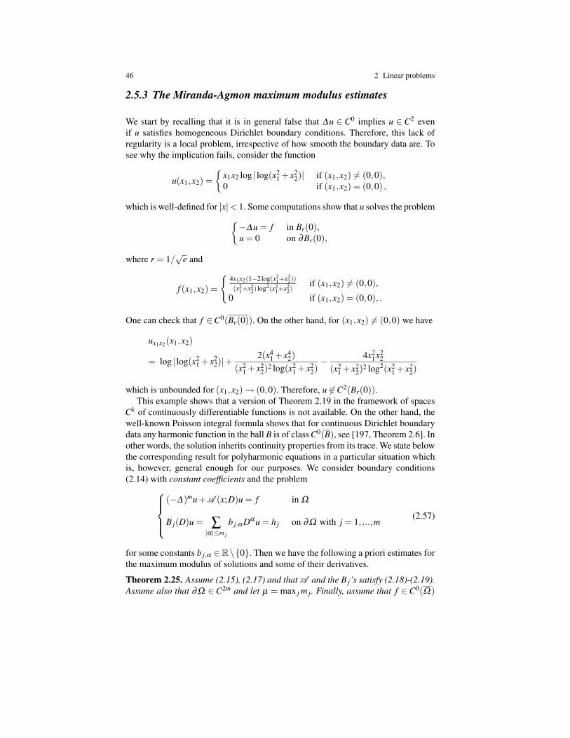
46 2 Linear problems
2.5.3 The Miranda-Agmon maximum modulus estimates
We start by recalling that it is in general false that ∆u ∈ C0 implies u ∈ C2 evenif u satisfies homogeneous Dirichlet boundary conditions. Therefore, this lack ofregularity is a local problem, irrespective of how smooth the boundary data are. Tosee why the implication fails, consider the function
u(x1,x2) =
x1x2 log | log(x21 + x2
2)| if (x1,x2) 6= (0,0),0 if (x1,x2) = (0,0) ,
which is well-defined for |x|< 1. Some computations show that u solves the problem−∆u = f in Br(0),u = 0 on ∂Br(0),
where r = 1/√
e and
f (x1,x2) =
4x1x2(1−2log(x2
1+x22))
(x21+x2
2) log2(x21+x2
2)if (x1,x2) 6= (0,0),
0 if (x1,x2) = (0,0), .
One can check that f ∈C0(Br(0)). On the other hand, for (x1,x2) 6= (0,0) we have
ux1x2(x1,x2)
= log | log(x21 + x2
2)|+2(x4
1 + x42)
(x21 + x2
2)2 log(x21 + x2
2)− 4x2
1x22
(x21 + x2
2)2 log2(x21 + x2
2)
which is unbounded for (x1,x2)→ (0,0). Therefore, u 6∈C2(Br(0)).This example shows that a version of Theorem 2.19 in the framework of spaces
Ck of continuously differentiable functions is not available. On the other hand, thewell-known Poisson integral formula shows that for continuous Dirichlet boundarydata any harmonic function in the ball B is of class C0(B), see [197, Theorem 2.6]. Inother words, the solution inherits continuity properties from its trace. We state belowthe corresponding result for polyharmonic equations in a particular situation whichis, however, general enough for our purposes. We consider boundary conditions(2.14) with constant coefficients and the problem
(−∆)mu+A (x;D)u = f in Ω
B j(D)u = ∑|α|≤m j
b j,α Dα u = h j on ∂Ω with j = 1, ...,m(2.57)
for some constants b j,α ∈R\0. Then we have the following a priori estimates forthe maximum modulus of solutions and some of their derivatives.
Theorem 2.25. Assume (2.15), (2.17) and that A and the B j’s satisfy (2.18)-(2.19).Assume also that ∂Ω ∈C2m and let µ = max j m j. Finally, assume that f ∈C0(Ω)
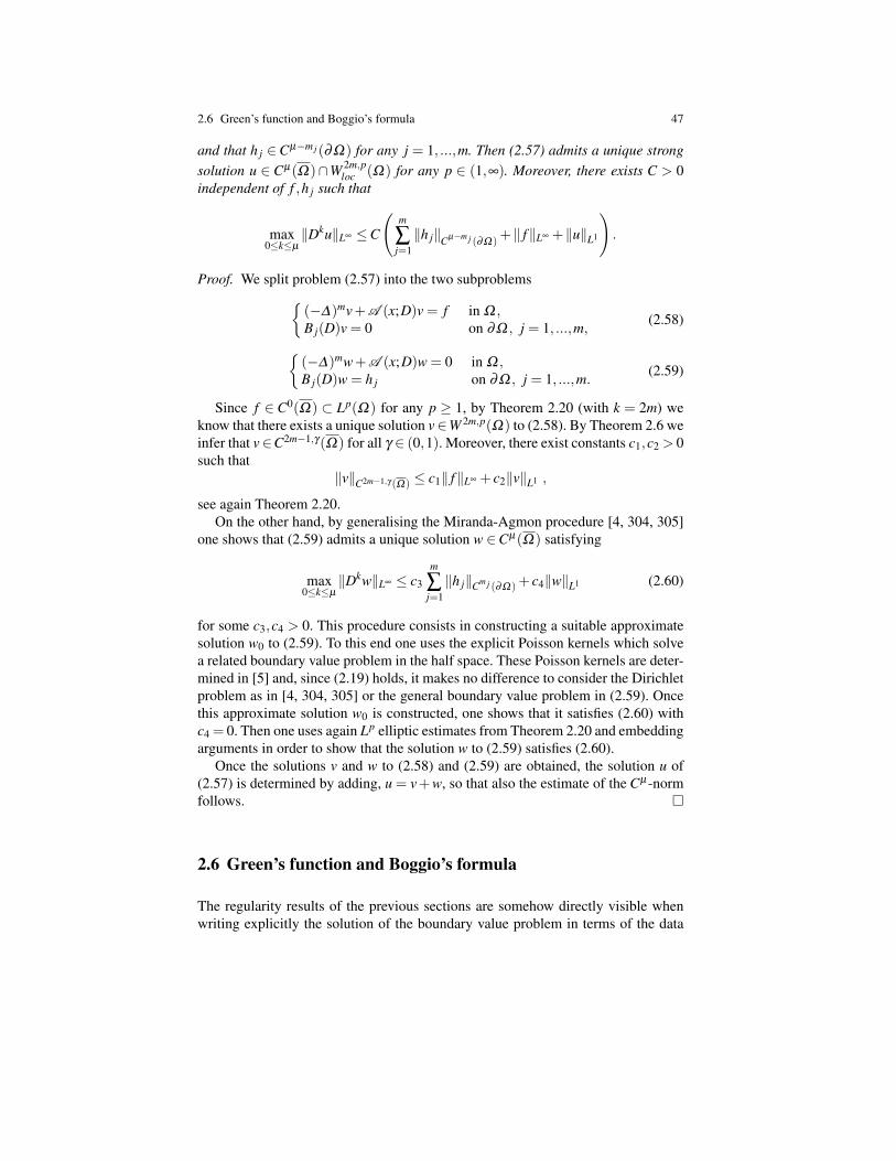
2.6 Green’s function and Boggio’s formula 47
and that h j ∈Cµ−m j(∂Ω) for any j = 1, ...,m. Then (2.57) admits a unique strongsolution u ∈ Cµ(Ω)∩W 2m,p
loc (Ω) for any p ∈ (1,∞). Moreover, there exists C > 0independent of f ,h j such that
max0≤k≤µ
‖Dku‖L∞ ≤C
(m
∑j=1‖h j‖Cµ−m j (∂Ω) +‖ f‖L∞ +‖u‖L1
).
Proof. We split problem (2.57) into the two subproblems(−∆)mv+A (x;D)v = f in Ω ,B j(D)v = 0 on ∂Ω , j = 1, ...,m,
(2.58)
(−∆)mw+A (x;D)w = 0 in Ω ,B j(D)w = h j on ∂Ω , j = 1, ...,m.
(2.59)
Since f ∈ C0(Ω) ⊂ Lp(Ω) for any p ≥ 1, by Theorem 2.20 (with k = 2m) weknow that there exists a unique solution v∈W 2m,p(Ω) to (2.58). By Theorem 2.6 weinfer that v∈C2m−1,γ(Ω) for all γ ∈ (0,1). Moreover, there exist constants c1,c2 > 0such that
‖v‖C2m−1,γ (Ω) ≤ c1‖ f‖L∞ + c2‖v‖L1 ,
see again Theorem 2.20.On the other hand, by generalising the Miranda-Agmon procedure [4, 304, 305]
one shows that (2.59) admits a unique solution w ∈Cµ(Ω) satisfying
max0≤k≤µ
‖Dkw‖L∞ ≤ c3
m
∑j=1‖h j‖Cm j (∂Ω) + c4‖w‖L1 (2.60)
for some c3,c4 > 0. This procedure consists in constructing a suitable approximatesolution w0 to (2.59). To this end one uses the explicit Poisson kernels which solvea related boundary value problem in the half space. These Poisson kernels are deter-mined in [5] and, since (2.19) holds, it makes no difference to consider the Dirichletproblem as in [4, 304, 305] or the general boundary value problem in (2.59). Oncethis approximate solution w0 is constructed, one shows that it satisfies (2.60) withc4 = 0. Then one uses again Lp elliptic estimates from Theorem 2.20 and embeddingarguments in order to show that the solution w to (2.59) satisfies (2.60).
Once the solutions v and w to (2.58) and (2.59) are obtained, the solution u of(2.57) is determined by adding, u = v+w, so that also the estimate of the Cµ -normfollows.
2.6 Green’s function and Boggio’s formula
The regularity results of the previous sections are somehow directly visible whenwriting explicitly the solution of the boundary value problem in terms of the data
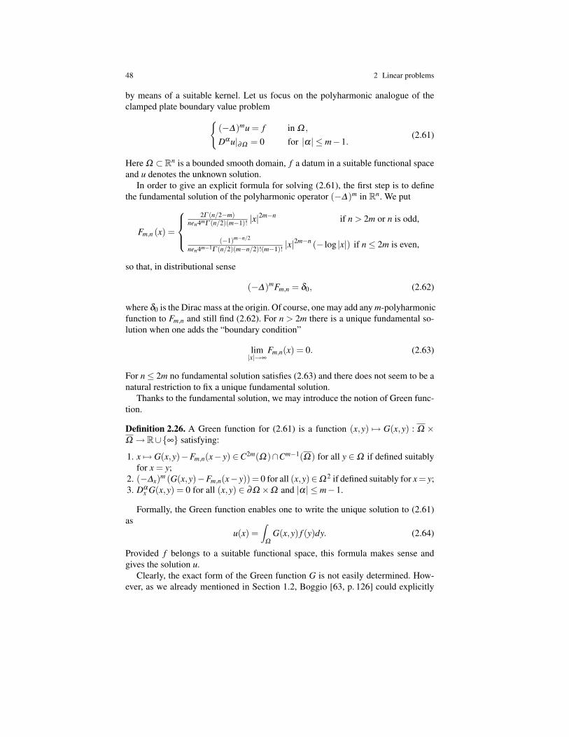
48 2 Linear problems
by means of a suitable kernel. Let us focus on the polyharmonic analogue of theclamped plate boundary value problem
(−∆)mu = f in Ω ,
Dα u|∂Ω = 0 for |α| ≤ m−1.(2.61)
Here Ω ⊂Rn is a bounded smooth domain, f a datum in a suitable functional spaceand u denotes the unknown solution.
In order to give an explicit formula for solving (2.61), the first step is to definethe fundamental solution of the polyharmonic operator (−∆)m in Rn. We put
Fm,n (x) =
2Γ (n/2−m)
nen4mΓ (n/2)(m−1)! |x|2m−n if n > 2m or n is odd,
(−1)m−n/2
nen4m−1Γ (n/2)(m−n/2)!(m−1)! |x|2m−n (− log |x|) if n≤ 2m is even,
so that, in distributional sense
(−∆)mFm,n = δ0, (2.62)
where δ0 is the Dirac mass at the origin. Of course, one may add any m-polyharmonicfunction to Fm,n and still find (2.62). For n > 2m there is a unique fundamental so-lution when one adds the “boundary condition”
lim|x|→∞
Fm,n(x) = 0. (2.63)
For n≤ 2m no fundamental solution satisfies (2.63) and there does not seem to be anatural restriction to fix a unique fundamental solution.
Thanks to the fundamental solution, we may introduce the notion of Green func-tion.
Definition 2.26. A Green function for (2.61) is a function (x,y) 7→ G(x,y) : Ω ×Ω → R∪∞ satisfying:
1. x 7→ G(x,y)−Fm,n(x− y) ∈C2m(Ω)∩Cm−1(Ω) for all y ∈Ω if defined suitablyfor x = y;
2. (−∆x)m (G(x,y)−Fm,n(x− y))= 0 for all (x,y)∈Ω 2 if defined suitably for x = y;3. Dα
x G(x,y) = 0 for all (x,y) ∈ ∂Ω ×Ω and |α| ≤ m−1.
Formally, the Green function enables one to write the unique solution to (2.61)as
u(x) =∫
Ω
G(x,y) f (y)dy. (2.64)
Provided f belongs to a suitable functional space, this formula makes sense andgives the solution u.
Clearly, the exact form of the Green function G is not easily determined. How-ever, as we already mentioned in Section 1.2, Boggio [63, p. 126] could explicitly
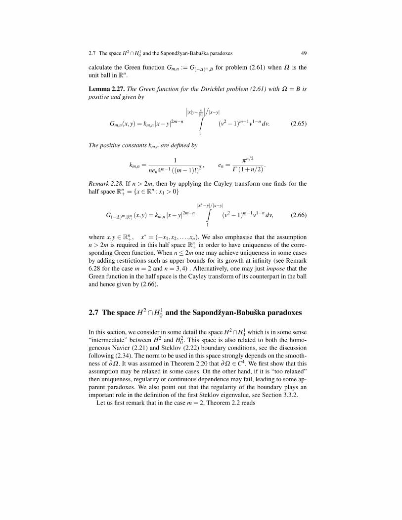
2.7 The space H2∩H10 and the Sapondzyan-Babuska paradoxes 49
calculate the Green function Gm,n := G(−∆)m,B for problem (2.61) when Ω is theunit ball in Rn.
Lemma 2.27. The Green function for the Dirichlet problem (2.61) with Ω = B ispositive and given by
Gm,n(x,y) = km,n |x− y|2m−n
∣∣∣|x|y− x|x|
∣∣∣/|x−y|∫1
(v2−1)m−1v1−n dv. (2.65)
The positive constants km,n are defined by
km,n =1
nen4m−1 ((m−1)!)2 , en =πn/2
Γ (1+n/2).
Remark 2.28. If n > 2m, then by applying the Cayley transform one finds for thehalf space Rn
+ = x ∈ Rn : x1 > 0
G(−∆)m,Rn+(x,y) = km,n |x− y|2m−n
|x∗−y|/|x−y|∫1
(v2−1)m−1v1−n dv, (2.66)
where x,y ∈ Rn+, x∗ = (−x1,x2, . . . ,xn). We also emphasise that the assumption
n > 2m is required in this half space Rn+ in order to have uniqueness of the corre-
sponding Green function. When n≤ 2m one may achieve uniqueness in some casesby adding restrictions such as upper bounds for its growth at infinity (see Remark6.28 for the case m = 2 and n = 3,4) . Alternatively, one may just impose that theGreen function in the half space is the Cayley transform of its counterpart in the balland hence given by (2.66).
2.7 The space H2∩H10 and the Sapondzyan-Babuska paradoxes
In this section, we consider in some detail the space H2∩H10 which is in some sense
“intermediate” between H2 and H20 . This space is also related to both the homo-
geneous Navier (2.21) and Steklov (2.22) boundary conditions, see the discussionfollowing (2.34). The norm to be used in this space strongly depends on the smooth-ness of ∂Ω . It was assumed in Theorem 2.20 that ∂Ω ∈C4. We first show that thisassumption may be relaxed in some cases. On the other hand, if it is “too relaxed”then uniqueness, regularity or continuous dependence may fail, leading to some ap-parent paradoxes. We also point out that the regularity of the boundary plays animportant role in the definition of the first Steklov eigenvalue, see Section 3.3.2.
Let us first remark that in the case m = 2, Theorem 2.2 reads
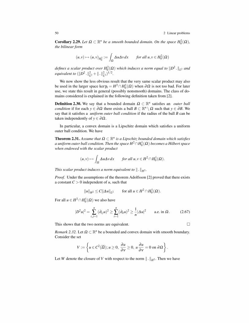
50 2 Linear problems
Corollary 2.29. Let Ω ⊂ Rn be a smooth bounded domain. On the space H20 (Ω),
the bilinear form
(u,v) 7→ (u,v)H20
:=∫
Ω
∆u∆vdx for all u,v ∈ H20 (Ω)
defines a scalar product over H20 (Ω) which induces a norm equal to ‖D2 .‖L2 and
equivalent to (‖D2 .‖2L2 +‖ .‖2
L2)1/2.
We now show the less obvious result that the very same scalar product may alsobe used in the larger space kerγ0 = H2∩H1
0 (Ω) when ∂Ω is not too bad. For lateruse, we state this result in general (possibly nonsmooth) domains. The class of do-mains considered is explained in the following definition taken from [2].
Definition 2.30. We say that a bounded domain Ω ⊂ Rn satisfies an outer ballcondition if for each y ∈ ∂Ω there exists a ball B ⊂ Rn \Ω such that y ∈ ∂B. Wesay that it satisfies a uniform outer ball condition if the radius of the ball B can betaken independently of y ∈ ∂Ω .
In particular, a convex domain is a Lipschitz domain which satisfies a uniformouter ball condition. We have
Theorem 2.31. Assume that Ω ⊂ Rn is a Lipschitz bounded domain which satisfiesa uniform outer ball condition. Then the space H2∩H1
0 (Ω) becomes a Hilbert spacewhen endowed with the scalar product
(u,v) 7→∫
Ω
∆u∆vdx for all u,v ∈ H2∩H10 (Ω).
This scalar product induces a norm equivalent to ‖ .‖H2 .
Proof. Under the assumptions of the theorem Adolfsson [2] proved that there existsa constant C > 0 independent of u, such that
‖u‖H2 ≤C‖∆u‖L2 for all u ∈ H2∩H10 (Ω).
For all u ∈ H2∩H10 (Ω) we also have
|D2u|2 =n
∑i, j=1
(∂i ju)2 ≥n
∑i=1
(∂iiu)2 ≥ 1n|∆u|2 a.e. in Ω . (2.67)
This shows that the two norms are equivalent.
Remark 2.32. Let Ω ⊂Rn be a bounded and convex domain with smooth boundary.Consider the set
V :=
u ∈C2(Ω); u≥ 0,∂u∂ν
≥ 0, u∂u∂ν
= 0 on ∂Ω
.
Let W denote the closure of V with respect to the norm ‖ .‖H2 . Then we have

2.7 The space H2∩H10 and the Sapondzyan-Babuska paradoxes 51∫
Ω
|D2u|2 dx≤∫
Ω
|∆u|2 dx for all u ∈W,
see [198, Theorem 2.1]. This inequality is somehow the converse of (2.67).
The assumptions on ∂Ω under which Theorem 2.31 holds are related to the so-called Sapondzyan or concave corner paradox. This paradox relies on the fact that,for some nonsmooth domains Ω , the linear Navier problem may have several dif-ferent solutions, according to the functional space where they are sought.
One way of getting the existence is through a “system solution” which belongsto H1
0 (Ω) as well as its Laplacian. A second type of solution is obtained usingKondratiev’s techniques in the space H2 ∩H1
0 (Ω). Note that, since ‖.‖ defined by‖u‖ := ‖∆u‖L2 is not a norm on H2 ∩H1
0 (Ω) when the domain has a reentrantcorner, one cannot directly apply the Lax-Milgram theorem. Indeed, Theorem 2.31may not hold if a uniform outer ball condition fails. The following example appearssuitable to illustrate this dichotomy in some detail.
Example 2.33. For α ∈( 1
2 π,π)
fix the domain
Ωα =(r cosϕ,r sinϕ) ∈ R2;0 < r < 1 and |ϕ|< α
.
Let f ∈ L2(Ωα) and consider the homogeneous Navier problem∆ 2u = f in Ωα ,u = 0 on ∂Ωα ,∆u = 0 on ∂Ωα \0.
(2.68)
We say that u is a system solution to (2.68) if u,∆u ∈ H10 (Ωα) and
−∆u = w and −∆w = f in Ωα ,u = 0 and w = 0 on ∂Ωα .
(2.69)
By applying twice the Lax-Milgram theorem in H10 (Ωα), this system solution, as a
solution to an iterated Dirichlet Laplace problem on a bounded domain, exists forany f ∈ L2(Ωα). Using [251] one finds that there also exists a solution in H2 ∩H1
0 (Ω) of (2.68), which indeed satisfies ∆u = 0 pointwise on ∂Ω \ 0. Since itssecond derivatives are square summable, let us call this the energy solution.
Next we consider a special function. For ρ = π
2αthe function vα defined by
vα(r,ϕ) =(r−ρ − rρ
)cos(ρϕ)
satisfies −∆vα = 0 in Ωα ,
vα = 0 on ∂Ωα\0.
Moreover, one directly checks that vα ∈ L2(Ωα) for ρ ∈( 1
2 ,1). Then there exists a
unique solution bα ∈ H10 (Ωα) of
52 2 Linear problems−∆bα = vα in Ωα ,
bα = 0 on ∂Ωα .
One has ∆bα 6∈ H10 (Ωα) and may check that bα 6∈ H2(Ωα). So we have found a
nontrivial solution to (2.68) with f = 0. This bα is neither a system solution nor anenergy solution. Let u be the system solution. Then the following holds:
1. For all c ∈ R we have uc := u+ cbα ∈ H10 (Ωα) and ∆uc ∈ L2(Ωα).
2. For all c ∈ R, the function uc satisfies (2.68). Using results in [318] one mayshow that in fact uc ∈C0(Ωα) and ∆uc ∈C0
loc(Ωα \0) whenever f ∈ L2(Ωα).3. One finds ∆uc ∈ H1
0 (Ωα) if and only if c = 0.4. For f ∈ L2(Ωα) let
cα( f ) :=−‖vα‖−2L2
∫Ωα
vαG−∆ ,Ωαf dx.
We have uc ∈ H2∩H10 (Ωα) if and only if c = cα( f ).
5. The energy solution to (2.68) is uc with c = cα( f ). Hence the system solution isdifferent from the energy solution whenever cα( f ) 6= 0.
Now let f be positive. A close inspection shows, see [320], that for the systemsolution the H2-regularity fails when cα( f ) 6= 0 while positivity holds true. On theother hand, the energy solution uc with c = cα( f ) has the appropriate regularity, butpositivity fails when α > 3
4 π and∫Ωα
(r−
πα − r
πα
)sin(
π
αϕ)G−∆ ,Ωα
f dx 6= 0.
For α ∈ ( 12 π, 3
4 π) there is only numerical evidence of sign-changing energy solu-tions. See Figure 2.1.
We now discuss in detail another famous paradox due to Babuska, also knownas the polygon-circle paradox. The starting point is a planar hinged plate Ω with aload f ∈ L2(Ω). This gives rise to the Steklov problem
∆ 2u = f in Ω ,
u = ∆u− (1−σ)κ∂u∂ν
= 0 on ∂Ω ,(2.70)
where κ denotes the curvature of the boundary and σ is the Poisson ratio. Problem(2.70) is considered both in the unit disk B and in the sequence (see Figure 1.3) ofinscribed regular polygons (Pm)⊂ B (m≥ 3) with corners(
cos(
2km
π
),sin
(2km
π
));k = 1, . . . ,m
.
Since the sides of Pm are flat, the curvature vanishes there and (2.70) becomes∆ 2u = f in Pm,u = ∆u = 0 on ∂Pm.
(2.71)
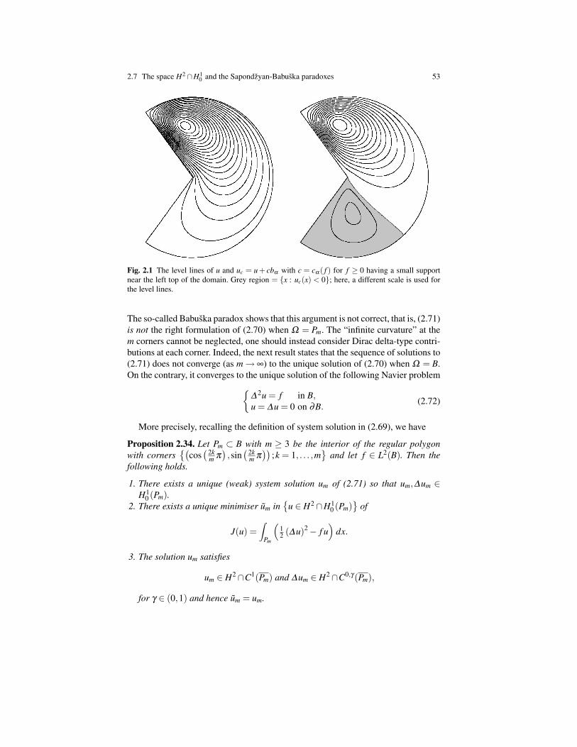
2.7 The space H2∩H10 and the Sapondzyan-Babuska paradoxes 53
Fig. 2.1 The level lines of u and uc = u + cbα with c = cα ( f ) for f ≥ 0 having a small supportnear the left top of the domain. Grey region = x : uc(x) < 0; here, a different scale is used forthe level lines.
The so-called Babuska paradox shows that this argument is not correct, that is, (2.71)is not the right formulation of (2.70) when Ω = Pm. The “infinite curvature” at them corners cannot be neglected, one should instead consider Dirac delta-type contri-butions at each corner. Indeed, the next result states that the sequence of solutions to(2.71) does not converge (as m→ ∞) to the unique solution of (2.70) when Ω = B.On the contrary, it converges to the unique solution of the following Navier problem
∆ 2u = f in B,u = ∆u = 0 on ∂B.
(2.72)
More precisely, recalling the definition of system solution in (2.69), we have
Proposition 2.34. Let Pm ⊂ B with m ≥ 3 be the interior of the regular polygonwith corners
(cos( 2k
m π),sin
( 2km π))
;k = 1, . . . ,m
and let f ∈ L2(B). Then thefollowing holds.
1. There exists a unique (weak) system solution um of (2.71) so that um,∆um ∈H1
0 (Pm).2. There exists a unique minimiser um in
u ∈ H2∩H1
0 (Pm)
of
J(u) =∫
Pm
(12 (∆u)2− f u
)dx.
3. The solution um satisfies
um ∈ H2∩C1(Pm) and ∆um ∈ H2∩C0,γ(Pm),
for γ ∈ (0,1) and hence um = um.
54 2 Linear problems
4. If we extend um by 0 on B\Pm and let u∞ be the solution of (2.72), then
limm→∞
‖um−u∞‖L∞(B) = 0.
Note that even if the identity of um and um may not seem very surprising, Exam-ple 2.33 shows that for domains with nonconvex corners these two solutions can bedifferent.Proof. 1. By the Lax-Milgram theorem, for any bounded domain Ω (in particular,if Ω = Pm) and any f ∈ L2(Ω) the Poisson problem
−∆w = f in Ω ,w = 0 on ∂Ω ,
(2.73)
has a unique (weak) solution in H10 (Ω). Similarly, one finds a unique solution in
H10 (Ω) to −∆u = w in Ω with u = 0 on ∂Ω . We apply this fact to the case where
Ω = Pm.2. The functional J is convex and coercive on H2∩H1
0 (Pm) in view of Theorem2.31 since the corner points of Pm all have angles less then π (i.e. Pm satisfies auniform outer ball condition). As the functional J is weakly lower semicontinuousand the closed unit ball in H2∩H1
0 (Pm) is weakly compact there exists a minimiser.The strict convexity gives uniqueness.
3. Invoking again [2] (or [240] since the Pm are convex), we know that the solutionof (2.73) in Pm with source in L2(Pm) lies in H2(Pm). Hence ∆um ∈ H2(Pm) and,by Theorem 2.6, ∆um ∈C0,γ(Pm) for all γ ∈ (0,1). In fact, by Kondratiev [251] onefinds that for a convex domain in two dimensions, with all corners having an openingangle less than or equal to α ∈
(π
2 ,π), the solution of (2.73) for f ∈ Lp(Ω) with
p < pα = 2α
2α−πlies in W 2,p(Ω). Hence for each Pm one finds that um ∈W 2,2+ε(Pm)
for 0≤ ε < 4m−4 . Theorem 2.6 then implies that um ∈C1(Pm).
4. It is sufficient to prove this result for f ≥ 0. For r ∈ (0,1) we compare thesolutions wr of
−∆w = f in Br,w = 0 on ∂Br.
Extend wr to B\Br by 0. Assuming f ≥ 0 and f ∈ L2(B) one finds that for 0 < r1 <r2 < 1 it holds that wr1 ≤ wr2 and moreover, that
lims→r
‖ws−wr‖L∞(B) = 0.
Indeed, if f ∈ L2(B), then ws,wr ∈C0,γ(B) and for s < r we find that−∆ (wr−ws) = 0 in Bs,wr−ws = wr on ∂Bs.
Since wr ∈C0,γ(B), this yields
‖wr‖L∞(Br\Bs) ≤C f |r− s|γ .

2.7 The space H2∩H10 and the Sapondzyan-Babuska paradoxes 55
By the maximum principle
‖wr−ws‖L∞(B) = ‖wr−ws‖L∞(Bs) ≤ ‖wr‖L∞(∂Bs) ≤C f |r− s|γ .
Again using the maximum principle and writing ur for the solution of (2.72) in Br(instead of B) we find
ur(x)≤ u1(x)≤ ur(x)+C f |1− r|γ . (2.74)
Two more applications of the maximum principle result in
urm(x)≤ um(x)≤ u1(x) (2.75)
with rm = cos(π/m) since Brm ⊂Pm ⊂B. The last claim follows by combining (2.74)and (2.75).
In order to emphasise the role played by smooth/nonsmooth boundaries in thisparadox, we prove
Proposition 2.35. Let Ω ⊂ R2 be a bounded domain with C2 boundary and let σ ∈(−1,1). If f ∈ L2(Ω), then there exists a unique minimiser uσ ∈ H2∩H1
0 (Ω) of
J(u) =∫
Ω
(12 (∆u)2 +(1−σ)
(u2
xy−uxxuyy)− f u
)dxdy.
If ∂Ω ∈C4, then uσ ∈ H4(Ω) and uσ satisfies∆ 2u = f in Ω ,
u = ∆u− (1−σ)κ∂u∂ν
= 0 on ∂Ω .(2.76)
Proof. Assume first that 0≤ σ < 1. Since the expression
12 (∆u)2 +(1−σ)
(u2
xy−uxxuyy)
= σ
2 (uxx +uyy)2 + 1−σ
2
(u2
xx +2u2xy +u2
yy)
is convex in the second derivatives of u, so is J. If −1 < σ < 0, following [331,Proposition 2.4] we note that
〈dJ(v1)−dJ(v2),v1− v2〉
=∫
Ω
((v1− v2)2
xx +(v1− v2)2yy +2σ(v1− v2)xx(v1− v2)yy
+ 2(1−σ)(v1− v2)2xy)
dxdy
≥ (1+σ)∫
Ω
((v1− v2)2
xx +(v1− v2)2yy +2(v1− v2)2
xy)dxdy
> 0
for all v1,v2 ∈ H2∩H10 (Ω) (v1 6= v2), where we used the simple inequality 2σab≥
σ(a2 +b2). Hence, also for −1 < σ < 0, the functional J is convex.

56 2 Linear problems
Then existence and uniqueness of a minimiser for J are obtained as in Proposition2.34. The minimiser u satisfies the weak Euler-Lagrange equation, that is∫
Ω
(∆u∆ϕ +(1−σ)(2uxyϕxy−uxxϕyy−uyyϕxx)− f ϕ
)dxdy = 0
for all ϕ ∈ H2 ∩H10 (Ω). Regularity arguments (see Theorem 2.20) show that for
∂Ω ∈C4 and f ∈ L2(Ω) the minimiser lies in H4(Ω). The integration by parts in(1.7) and (1.8) show that uσ satisfies (2.76).
By combining Propositions 2.34 and 2.35 we may now better explain the Babuskaparadox. Assume that f ∈ L2(B) and let σ 6= 1. If u∞ is as in Proposition 2.34 anduσ is as in Proposition 2.35, then
u∞ ≡ uσ in B ⇐⇒ ∂u∞
∂ν≡ 0 on ∂B.
But if 0 6= f ≥ 0, then the maximum principle implies−∆u∞ > 0 and u∞ > 0 whereasHopf’s boundary point Lemma even gives ∂u∞
∂ν< 0 on ∂B and hence u∞ 6= uσ .
Babuska considered the case where f = 1 in B. This simple source allows us tocompute all the functions involved. The solution to (2.76) with f = 1 on B is theradially symmetric function
uσ (x) =(5+σ)− (6+2σ) |x|2 +(1+σ) |x|4
64(1+σ).
The limit u∞ in Babuska’s example, defined by u∞(x) = limm→∞ um(x) equalsuσ=1(x), namely
u∞(x) =364− 1
16|x|2 +
164|x|4 ,
see also [401, p. 499] and [135].
-1 -0.5 0.5 1
0.02
0.04
0.06
0.08
Fig. 2.2 The example of Babuska: Ω = B and f = 1. The solutions uσ to (1.10) depend on σ ; fromtop to bottom the solutions for σ = 0, .3, .5 and 1. The solution for σ = 1 is the limit of um fromthe regular m-polygon with m→ ∞.
2.8 Bibliographical notes 57
2.8 Bibliographical notes
Ellipticity and the complementing condition are well explained in [5], see also Sec-tion 1 of Chapter 2 in [275]. The polynomial Lm representing the differential op-erator is taken from [5, Section I.1], see also Section 1.1 of Chapter 2 in [275].For boundary conditions that do not satisfy assumption (2.15) we refer again to [5].The complementing condition is sometimes also called Lopatinski-Shapiro condi-tion and may be defined in an equivalent way, see [416, Section 11]. Concerningassumption (2.17), we refer to [416, Theorem 13.1] for a general statement relatingellipticity, the complementing condition, regularity results, Fredholm theory and apriori estimates.
More results about Sobolev spaces may be found in the monographs by Adams[1], Maz’ya [291] and Lions-Magenes [275]. All the embedding theorems in Section2.2.2 may be derived from [1, Theorems 5.4 and 6.2] whereas for the scalar productin Hm(Ω) see [275, Theoreme 1.1]. Theorem 2.31 is taken from [80] and Theorem2.7 is taken from [1, Theorem 5.23].
The material from Section 2.4 is taken from Section 9 of Chapter 2 in [275] andfrom [416]. Theorem 2.13 is a variant of Green’s formula, see [416, Theorem 14.8].A Hilbert triple as in Definition 2.14 is a particular case of a Gelfand triple, see [416,Definition 17.1]. The coercivity condition in (2.41) is given in Hm(Ω), the frame-work of our setting; it is taken from [275, Definition 2.9.1]. Agmon’s conditionwhich ensures the coercivity of the bilinear form Ψ(u,v) was originally stated in[3]; we also refer to Theorem 9.3 of Chapter 2 in [275] and to [416, Section 18] forequivalent formulations. Theorem 2.16 is a direct consequence of the Lax-Milgramtheorem, see [416, Theorem 17.10]. Existence, uniqueness and regularity results for(2.2)-(2.14) with data in the Hilbert spaces Hs with s ∈R (possibly also non integerand negative) are studied in full detail in [275]; in particular, we refer to Remark 7.2of Chapter 2 in [275] for a statement including all possible cases. Theorem 2.19 iscontained in [5, Theorem 9.3] whereas Theorem 2.20 is contained in [5, Theorem15.2]. Theorem 2.22 and the extension of Corollary 2.23 to all k ≥ 2 are justifiedby [5, Theorem 15.3’]. Theorem 2.25 follows as a by-product of Theorems 2.6 and2.20 on one hand and maximum modulus estimates for solutions of higher orderelliptic equations on the other hand. This second tool was introduced by Miranda[304, 305] for higher order problems in the plane and subsequently generalised byAgmon [4] in any space dimension. We also refer to [377] for a simple sketch ofthe proof. Finally, let us mention that partial extensions and counterexamples toTheorem 2.25 in nonsmooth domains may be found in works by Pipher-Verchota[337, 338], Maz’ya-Rossmann [290], Mayboroda-Maz’ya [284, 285] and referencestherein. Lemma 2.27 is a fundamental contribution by Boggio [63] and is one of themost frequently used results in this monograph. Results on Green’s functions mayalso be found in the monograph [21]. As for Lp-theory of higher-order elliptic op-erators and underlying kernel estimates one may also see the survey article [129]by Davies. Theorem 2.31 is a straightforward consequence of results by Adolfsson[2], see also [237, 238] for related results. Concerning the Sapondzyan paradox, werefer to the original paper [357] and to more recent results on “multiple” solutions
58 2 Linear problems
in [320]. Babuska [28] noticed first that by approximating a curvilinear domain bypolygons the approximating solutions would not converge to the solution on thecurvilinear domain. Engineering approaches to the Babuska or polygon-circle para-dox can be found in [241, 314, 354]. A mathematical approach can be found in thework by Maz’ya and Nazarov [292, 293]. These authors dealt with the paradox by acareful asymptotic analysis of the boundary layer and the contribution of the cornersin this. Part of their results are based on Γ -convergence results from [422]. More re-cently, Davini [134] again uses Γ -convergence to find a correct approximation. Hefocuses on numerical methods that avoid the pitfall of this paradox. Most part of thematerial in Section 2.7 is taken from [387].
Chapter 3Eigenvalue problems
For quite general second order elliptic operators one may use the maximum princi-ple and the Kreın-Rutman theorem to show that the eigenfunction corresponding tothe first eigenvalue has a fixed sign. It is then a natural question to ask if a similarresult holds for higher order Dirichlet problems where a general maximum principleis not available. A partial answer is that a Kreın-Rutman type argument can still beused whenever the boundary value problem is positivity preserving. We will also ex-plain in detail an alternative dual cone approach. Both these methods have their ownadvantages. The Kreın-Rutman approach shows under fairly weak assumptions thatthere exists a real eigenvalue and, somehow as a byproduct, one finds that the eigen-value and the corresponding eigenfunction are positive. It applies in particular tonon-selfadjoint settings. The dual cone decomposition only applies in a selfadjointframework in a Hilbert space, where the existence of eigenfunctions is well-known.But in this setting it provides a very simple proof for positivity and simplicity of thefirst eigenfunction. A further quality of this method is that it applies also to somenonlinear situations as we shall see in Chapter 7.
We conclude this first part of the chapter with some further remarks on the con-nection between the positivity preserving property of the Dirichlet problem and thefixed sign property of the first eigenfunction. In particular, we show that the latterproperty, as well as the simplicity of the first eigenvalue, may fail.
Then we turn to the minimisation of the first Dirichlet eigenvalue of the bihar-monic operator among domains of fixed measure and we show that, in dimensionsn = 2 and n = 3, the ball achieves the minimum. We also consider two further eigen-value problems, the buckling load of a clamped plate and Steklov eigenvalues. Upto some regularity to be proved, a quite hard open problem, the disk minimises thebuckling load among planar domains of given measure. For the Steklov problem wefirst study in detail the whole spectrum and then we show that an optimal shape ofgiven measure which minimises the first eigenvalue does not exist.
59
60 3 Eigenvalue problems
3.1 Dirichlet eigenvalues
Here we consider the eigenvalue problem(−∆)mu = λu , u 6≡ 0 in Ω ,
Dα u|∂Ω = 0 for |α| ≤ m−1(3.1)
on a given bounded domain Ω ⊂Rn (n≥ 2). The first eigenvalue of (3.1) is definedas
Λm,1(Ω) = minu∈Hm
0 (Ω)\0
‖u‖2Hm
0
‖u‖2L2
. (3.2)
In this section we discuss several problems related to (3.1) and to its first eigenvalue.We start by showing that the corresponding eigenfunction is of one sign wheneverthe problem
(−∆)mu = f in Ω ,
Dα u|∂Ω = 0 for |α| ≤ m−1(3.3)
is positivity preserving, see Definition 3.1 below. This statement can be obtained intwo different ways, either with a somehow standard Kreın-Rutman type argumentor with a decomposition in dual cones which we discuss in detail. Next, we discussthe positivity of the first eigenfunction and its failure in general and we end up withthe minimisation of the first eigenvalue among domains of given measure.
3.1.1 A generalised Kreın-Rutman result
The Kreın-Rutman theorem, which can be considered to have its roots in Jentzsch’stheorem, appears in many forms with many different and partially overlapping con-ditions but none of the classical versions are optimal for the solution operator of anelliptic boundary value problem. The main restriction is the necessity of having apositive cone with an open interior, see [257, Theorems 6.2 and 6.3]. As we shallsee, this restriction could be removed after a profound result of de Pagter [136].
Consider the linear problem (3.3) and the following notion of positivity preserv-ing.
Definition 3.1. We say that (3.3) has a positivity preserving property when the fol-lowing holds for all u and f satisfying (3.3):
f ≥ 0⇒ u≥ 0.
In case that a Green function exists, the positivity preserving property holds trueif and only if this Green function is nonnegative. We now establish that if (3.3) ispositivity preserving then a Kreın-Rutman result allows one to verify that the firsteigenvalue for (3.1) is simple and corresponds to an eigenfunction of fixed sign.
3.1 Dirichlet eigenvalues 61
Let us shortly introduce some terminology.
Definition 3.2. An ordered Banach space (E,‖ .‖ ,≥) is called a Banach lattice if:
• the least upper bound of two elements in E lies again in E:
f ,g ∈ E implies f ∨g := infh ∈ E;h≥ f and h≥ g ∈ E;
• the ordering of positive elements is preserved by the norm: setting | f |= f ∨(− f )it holds for all f ,g ∈ E that | f | ≤ |g| implies ‖ f‖ ≤ ‖g‖.
A linear subspace A⊂ E is called a lattice ideal if
| f | ≤ |g| and g ∈ A implies f ∈ A.
We call A invariant under the operator T : E → E if T (A)⊂ A.
We can now give a statement which improves the classical Kreın-Rutman theo-rem, see [257].
Theorem 3.3. Let E be a Banach lattice with dim(E) > 1 and let T : E → E be alinear operator satisfying:
• T is compact;• T is positive: T (K )⊂K where K is the positive cone in E;• T is irreducible: 0 and E are the only closed lattice ideals invariant under T .
Then the spectral radius ρ of T is strictly positive and there exists v ∈K \0 withT v = ρv. Moreover, the algebraic multiplicity of ρ is one, all other eigenvalues ρ
satisfy |ρ|< ρ and no other eigenfunction is positive.
By Lemma 2.27 we know that the Green function in the ball B is positive sothat problem (3.3) has a positivity preserving property whenever Ω = B. In fact,Theorem 3.3 applies to any domain Ω where the corresponding Green function GΩ
is strictly positive. In this case, one takes E = L2(Ω) or E = v ∈C(Ω); v|∂Ω = 0and T as the solution operator for (3.3). Since for each x ∈ Ω the Green functionGΩ (x, .) is strictly positive on Ω except for a set of measure 0 it follows in bothsettings that T is irreducible.
3.1.2 Decomposition with respect to dual cones
We state and discuss here an abstract result due to Moreau [311] about the decom-position of a Hilbert space H into dual cones; we recall that K ⊂ H is a cone ifu ∈ K and a ≥ 0 imply that au ∈ K . In order to exploit the full power of thisdecomposition, we also establish a generalised Boggio result. This will be used inseveral different points of this monograph. Finally, we give a first simple applicationof this decomposition to a capacity problem.
62 3 Eigenvalue problems
It was Miersemann [301] who first observed that the dual cone decompositioncould be quite helpful in the context of fourth order elliptic equations. In the nextsection we show how this method can be used to prove simplicity and positivity ofthe first eigenfunction of (3.1) in a ball. Moreover, this decomposition will turn outto be quite useful in a number of semilinear problems considered in this monograph.
Theorem 3.4. Let H be a Hilbert space with scalar product (., .)H . Let K ⊂ H bea closed convex nonempty cone. Let K ∗ be its dual cone, namely
K ∗ = w ∈ H; (w,v)H ≤ 0 for all v ∈K .
Then for any u ∈ H there exists a unique (u1,u2) ∈K ×K ∗ such that
u = u1 +u2 , (u1,u2)H = 0. (3.4)
In particular, ‖u‖2H = ‖u1‖2
H +‖u2‖2H .
Moreover, if we decompose arbitrary u,v ∈ H according to (3.4), namely u =u1 +u2 and v = v1 + v2, then we have that
‖u− v‖2H ≥ ‖u1− v1‖2
H +‖u2− v2‖2H .
In particular, the projection onto K is Lipschitz continuous with constant 1.
Proof. For a given u ∈ H, we prove separately existence and uniqueness of a de-composition satisfying (3.4).
Existence. Let u1 be the projection of u onto K defined by
‖u−u1‖= minv∈K
‖u− v‖
and let u2 := u−u1. Then for all t ≥ 0 and v ∈K one has
‖u−u1‖2H ≤ ‖u− (u1 + tv)‖2
H = ‖u−u1‖2H −2t(u−u1,v)H + t2‖v‖2
H
so that2t(u2,v)H ≤ t2‖v‖2
H . (3.5)
Dividing by t > 0 and letting t 0, (3.5) yields (u2,v)H ≤ 0 for all v ∈K so thatu2 ∈K ∗. Choosing v = u1 also allows for taking t ∈ [−1,0) in (3.5), so that dividingby t < 0 and letting t 0 yields (u2,u1)H ≥ 0 which, combined with the just provedconverse inequality, proves that (u2,u1)H = 0.
Lipschitz continuity. From the two inequalities (u1,v2)H ≤ 0 and (v1,u2)H ≤ 0and by orthogonality, we obtain
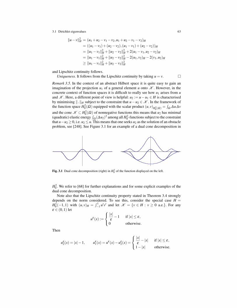
3.1 Dirichlet eigenvalues 63
‖u− v‖2H = (u1 +u2− v1− v2,u1 +u2− v1− v2)H
= ((u1− v1)+(u2− v2),(u1− v1)+(u2− v2))H
= ‖u1− v1‖2H +‖u2− v2‖2
H +2(u1− v1,u2− v2)H
= ‖u1− v1‖2H +‖u2− v2‖2
H −2(u1,v2)H −2(v1,u2)H
≥ ‖u1− v1‖2H +‖u2− v2‖2
H
and Lipschitz continuity follows.Uniqueness. It follows from the Lipschitz continuity by taking u = v.
Remark 3.5. In the context of an abstract Hilbert space it is quite easy to gain animagination of the projection u1 of a general element u onto K . However, in theconcrete context of function spaces it is difficult to really see how u1 arises from uand K . Here, a different point of view is helpful: u2 := u−u1 ∈ H is characterisedby minimising ‖ .‖H subject to the constraint that u−u2 ∈K . In the framework ofthe function space H2
0 (Ω) equipped with the scalar product (u,v)H20 (Ω) =
∫Ω
∆u∆v
and the cone K ⊂ H20 (Ω) of nonnegative functions this means that u2 has minimal
(quadratic) elastic energy∫
Ω(∆u2)2 among all H2
0 -functions subject to the constraintthat u−u2≥ 0, i.e. u2≤ u. This means that one seeks u2 as the solution of an obstacleproblem, see [248]. See Figure 3.1 for an example of a dual cone decomposition in
Fig. 3.1 Dual cone decomposition (right) in H20 of the function displayed on the left.
H20 . We refer to [68] for further explanations and for some explicit examples of the
dual cone decomposition.Note also that the Lipschitz continuity property stated in Theorem 3.4 strongly
depends on the norm considered. To see this, consider the special case H =H1
0 (−1,1) with (u,v)H =∫ 1−1 u′v′ and let K = v ∈ H : v ≥ 0 a.e.. For any
ε ∈ (0,1) let
uε(x) :=
|x|ε−1 if |x| ≤ ε,
0 otherwise.
Then
uε2(x) = |x|−1, uε
1(x) = uε(x)−uε2(x) =
|x|ε−|x| if |x| ≤ ε,
1−|x| otherwise.
64 3 Eigenvalue problems
Therefore, uε → 0 in L2(−1,1) as ε 0, while uε1 → 1−|x| and uε
2 ≡ |x|−1. Thisshows that the decomposition in H1
0 is not continuous with respect to the L2-norm.
Let us now explain how we are planning to use the decomposition in Theorem3.4. We will take H as a Hilbertian functional space (L2, H2, D2,2 . . .) and
K = u ∈ H; u≥ 0 a.e..
If H = L2(Ω), then K ∗ =−K and Theorem 3.4 simply yields
u = u+−u− for all u ∈ L2(Ω).
If H = H10 (Ω), in order to characterise K ∗ we seek v ∈ H1
0 (Ω) such that∫Ω
∇u∇vdx≤ 0 for all u ∈K .
This means that v is weakly subharmonic (formally,∫
Ωu∆v≥ 0) and therefore
K ∗ = v ∈ H10 (Ω); v is weakly subharmonic(−K .
Note that although∫
Ω∇u+∇u− = 0, the decomposition obtained here is different
from u = u+−u−.In higher order Sobolev spaces the decomposition u = u+−u− is no longer ad-
missible because if u ∈ Hm (m ≥ 2) then, in general, u+,u− 6∈ Hm. In some situa-tions the decomposition into dual cones may substitute the decomposition into pos-itive and negative part. In order to facilitate and strengthen the application of Theo-rem 3.4 to higher order Sobolev spaces, we generalise Boggio’s principle (Lemma2.27) to weakly subpolyharmonic functions in suitable domains. Let us consideragain K = v ∈ Hm
0 (Ω); v≥ 0 a.e. in Ω (or v ∈Dm,2(Ω) if Ω is unbounded andn > 2m), then
K ∗ =
w ∈ Hm0 (Ω); (w,v)Hm
0≤ 0 for all v ∈K
.
Hence, K ∗ = v ∈ Hm0 (Ω); (−∆)mv ≤ 0 weakly. In some cases, we have that
K ∗ ⊂−K .
Proposition 3.6. Assume that either Ω = BR (a ball of radius R), or Ω = Rn+, or
Ω = Rn; if Ω is unbounded, we also assume that n > 2m. Assume that w ∈ L2(Ω)is a weak subsolution of the polyharmonic Dirichlet problem, namely∫
Ω
w(−∆)mudx≤ 0 for all u ∈K ∩H2m∩Hm0 (Ω) ;
theneither w≡ 0 or w < 0 a.e. in Ω . (3.6)
In particular, (3.6) holds for all w ∈K ∗.
3.1 Dirichlet eigenvalues 65
Proof. We only prove the result in the case where Ω = B (the unit ball), the remain-ing cases being similar. Assuming n > 2m, for the half space it suffices to use (2.66)instead of (2.65) whereas for the whole space one takes the fundamental solution of(−∆)m.
Take any ϕ ∈K ∩C∞c (B) and let vϕ be the unique (classical) solution of
(−∆)mvϕ = ϕ in B,Dα vϕ = 0 on ∂B for |α| ≤ m−1.
Then by the classical Boggio’s principle (Lemma 2.27) we infer that vϕ ∈ K .Hence, vϕ is a possible test function for all such ϕ and therefore∫
Bwϕ dx =
∫B
w(−∆)mvϕ dx≤ 0 for all ϕ ∈K ∩C∞c (B).
This shows that w ≤ 0 a.e. in B. Assume that w 6< 0 a.e. in B and let φ denote thecharacteristic function of the set x ∈ B; w(x) = 0 so that φ ≥ 0, φ 6≡ 0. Let v0 bethe unique (a.e.) solution of the problem
(−∆)mv0 = φ in B,Dα v0 = 0 on ∂B for |α| ≤ m−1.
Then by Corollary 2.21 and Theorem 2.6, we know that
v0 ∈
(⋂q≥1
W 2m,q(B)
)⊂C2m−1(B)
and again by Boggio’s principle we have v0 > 0 in B. One also reads from Boggio’sformula (2.65) that (− ∂
∂ν)mv0 > 0 on ∂B, see Theorem 5.7 below. We infer that for
all v∈C2m(B)∩Hm0 (B) there exist t1 ≤ 0≤ t0 such that v+ t0v0 ≥ 0 and v+ t1v0 ≤ 0
in B. This, combined with the fact that∫B
w(−∆)mv0 dx =∫w=0
wdx = 0,
enables us to show that both
0≤∫
Bw(−∆)m(v+ t0v0)dx =
∫B
w(−∆)mvdx,
0≥∫
Bw(−∆)m(v+ t1v0)dx =
∫B
w(−∆)mvdx.
Hence, we have for all v ∈C2m(B)∩Hm0 (B)∫
Bw(−∆)mvdx = 0.
66 3 Eigenvalue problems
We need to show that C2m(B)∩Hm0 (B) is dense in H2m∩Hm
0 (B). For this purpose,take any function U ∈ H2m ∩Hm
0 (B) and put f := (−∆ m)U . We approximate f inL2(B) by C∞(B)–functions fk and solve (−∆ m)Uk = fk in B under homogeneousDirichlet boundary conditions. We then even have Uk ∈ C∞(B), and by L2–theory(see Corollary 2.21) it holds that ‖Uk−U‖H2m → 0 as k → ∞.
By the previous statement we may now conclude that∫B
w(−∆)mvdx = 0 for all v ∈ H2m∩Hm0 (B).
Since w ∈ L2(B), we may take as v ∈ H2m ∩Hm0 (B) the solution of (−∆)mv = w
under homogeneous Dirichlet boundary conditions. This finally yields w≡ 0.
We conclude this section with a first simple application of Theorem 3.4. We showthe positivity of the potential in the second order capacity problem. Given a boundeddomain Ω ⊂ Rn (n > 4) we define its second order capacity as
cap(Ω) = inf∫
Rn|∆u|2 dx; u ∈D2,2(Rn), u≥ 1 a.e. in Ω
.
Using Theorem 3.4 we can show that the potential (the minimiser) u is nonnegative.Let H = D2,2(Rn) and let K = u ∈ H : u ≥ 0 a.e. in Rn. If u is sign-changing,let u = u1 +u2 with u1 ∈K and u2 ∈K ∗ \0 be its decomposition according toTheorem 3.4. Then by Proposition 3.6 we know that u2 ≤ 0. Hence, u1 ≥ 1 in Ω sothat u1 is an admissible function. Moreover,∫
Rn|∆u|2 dx =
∫Rn|∆u1|2 dx+
∫Rn|∆u2|2 dx >
∫Rn|∆u1|2 dx.
This contradicts the minimality of u among admissible functions.
3.1.3 Positivity of the first eigenfunction
In this section we study positivity of the first eigenfunction of (3.1) by means ofthe just explained dual cone decomposition. As already mentioned in Section 3.1.1,whenever we have a positivity preserving solution operator, a Kreın-Rutman resultyields a positive first eigenfunction with the uniqueness properties stated in Theo-rem 3.3. In our special self-adjoint situation, the dual cone decomposition yields adirect and simpler proof. Moreover, this strategy can also be exploited for semilinearproblems, see e.g. Lemma 7.22 and Theorem 7.58.
Theorem 3.7. If Ω = B⊂ Rn, then the first eigenvalue
Λm,1 = infHm
0 (B)\0
‖u‖2Hm
0
‖u‖2L2
. (3.7)

3.1 Dirichlet eigenvalues 67
of (3.1) is simple and the corresponding first eigenfunction u is of one sign.
Proof. Let H = Hm0 (B) and let K = u ∈ H : u ≥ 0 a.e. in B. For contradiction,
assume that u changes sign. Then according to Theorem 3.4, we decompose u =u1 +u2, u1 ∈K \0, u2 ∈K ∗ \0. By Proposition 3.6, we have u2 < 0 a.e. in B.Replacing u with the positive function u1− u2 would strictly increase the L2-normwhile by orthogonality we have ‖u1 +u2‖2
H = ‖u1−u2‖2H . The ratio would strictly
decrease, a contradiction.Since a minimiser u ≥ 0 solves (−∆)mu = Λm,1u ≥ 0 we have u > 0 by Propo-
sition 3.6. By contradiction, assume now that (3.7) admits two linearly independentpositive minimisers u and v. Then w = u + αv (for a suitable α < 0) is a sign-changing minimiser, contradiction!
For m = 1 the very same technique used in Theorem 3.7 works in any boundeddomain Ω if we wish to show that the first eigenvalue of −∆ in H1
0 (Ω) is simpleand that the corresponding eigenfunction is of one sign. On the other hand, the L2-norm remains constant if we replace u+− u− with u+ + u−. So, for this problem,the decomposition into dual cones works directly, whereas the usual decompositioninto positive and negative parts does not prove simplicity of the first eigenvalue norfixed sign of the first eigenfunction without a further regularity argument.
Theorem 3.7 applies to any bounded domain Ω 6= B with a positive Green func-tion also for m ≥ 2. Note that the positivity preserving property (positivity of theGreen function) implies fixed sign of the first eigenfunction to (3.1) but the con-verse implication does not hold in general. One can then wonder whether a positivefirst eigenfunction can be obtained also for domains which fail to have the positiv-ity preserving property, see Definition 3.1. The answer is delicate and negative ingeneral.
Let us quickly outline what is known for sign-changing first eigenfunctions of∆ 2u = λu , u 6≡ 0 in Ω ,
u = |Du|= 0 on ∂Ω .(3.8)
Basically, only this biharmonic eigenvalue problem on bounded domains has beenconsidered so far. Concerning (3.8) it is proven in [212] that for an appropriately de-fined family of perturbations starting from the ball the positivity preserving propertyfails to hold strictly before the first eigenfunction loses its fixed sign. So, the con-verse implication on ellipses as mentioned above is not true, see also Remark 6.4.It does not seem to be rigorously proven yet that the sign of the first eigenfunctionchanges on ellipses with a large ratio but there exists numerical evidence.
The first example of a sign-changing first eigenfunction is due to Coffman [107]and deals with squares.
Theorem 3.8. For Ω = (0,1)2 problem (3.8) has a sign-changing first eigenfunc-tion.
Independently of previous results in [111], Kozlov-Kondratiev-Maz’ya [252]proved that domains in any space dimension whose boundaries contain suitable

68 3 Eigenvalue problems
cones also have a sign-changing first eigenfunction for (3.8). Their results covera class of elliptic operators of order 2m under Dirichlet boundary conditions. Theirproof is based on a result which ensures the absence of zeros of infinite order at thevertex of a cone, for nontrivial nonnegative local solutions of the inequality Au≤ 0,where A is an elliptic differential operator with real coefficients. Moreover, they con-structed a sequence of smooth convex domains that exhaust the cone and since thecorresponding first eigenfunctions are proven to converge to the sign-changing firsteigenfunction in the cone the same holds eventually for the approximating domains.
A main assumption that often appears is the convexity of Ω . From Theorem3.8 and the numerical evidence on eccentric ellipses it is clear that this assumptionwill not be sufficient to ensure positivity of the first eigenfunction. Ellipses suggestthat, possibly, a suitable upper bound for the ratio between the radii of the largestinscribed ball in Ω and the largest filling balls of Ω might yield a sufficient conditionfor a positive eigenfunction. We recall that B is a filling ball for Ω if Ω is the unionof translated B. Clearly, for any bounded domain this ratio is always larger than orequal to 1. An interesting family of domains in this sense are elongated disks, theso-called stadiums, where the radius of the largest inscribed ball equals the radius ofthe largest filling ball. Numerical approximations of the first eigenfunction on sucha domain always resulted in functions apparently of fixed sign.
Fig. 3.2 Stadium-like domains seem to have a positive first eigenfunction in the Dirichlet bihar-monic case.
Domains which are far from being convex are domains with holes. The standardexamples are the annuli
Aε = (x,y) ∈ R2; ε2 < x2 + y2 < 1 with 0 < ε < 1.
For these domains, Coffman-Duffin-Shaffer [109, 110, 155] proved the followingsomehow surprising statement.
Theorem 3.9. Let Ω = Aε for some ε ∈ (0,1) and consider problem (3.8). Thereexists ε0 > 0 such that the following holds.
1. If ε < ε0, then the first eigenvalue has multiplicity two. There exist two indepen-dent eigenfunctions for this first eigenvalue with diametral nodal lines.
2. If ε = ε0, then the first eigenvalue has multiplicity three. There exists a positiveeigenfunction for this eigenvalue and there are two independent eigenfunctionswith diametral nodal lines.

3.1 Dirichlet eigenvalues 69
3. If ε > ε0, then the first eigenvalue has multiplicity one and the correspondingeigenfunction is of fixed sign.
It is not surprising that a large hole yields a positive eigenfunction since the do-main becomes somehow close to an infinite strip with periodic boundary conditionsw.r.t. the unbounded direction, where the first eigenfunction in the appropriate func-tional space depends only on one variable and is positive.
Even more, numerical experiments indicate that there exist starshaped domains,where the first eigenfunction is anti-symmetric with respect to a nodal line and hencesign-changing. See [76] and Figure 3.3 which shows the first and second eigenfunc-tion for such a domain.
Fig. 3.3 On the left the first eigenfunction for the clamped biharmonic eigenvalue problem on an8-shaped domain which is sign-changing. On the right the second eigenfunction which is (almost)positive.
3.1.4 Symmetrisation and Talenti’s comparison principle
Let Λ1,1(Ω) denote the first Dirichlet eigenvalue for −∆ in a bounded domain Ω ⊂Rn, see (3.2) with m = 1. The celebrated Faber-Krahn [162, 253, 254] inequalitystates that if one considers the map Ω 7→ Λ1,1(Ω) in dependence of domains Ω
having all the same measure en as the unit ball B, its minimum is achieved preciselyfor Ω = B and, moreover, balls of radius 1 are the only minimisers. The crucial toolto prove this statement is symmetrisation. We recall here some basic facts about thismethod.
In 1836, Jacob Steiner noticed that symmetrisation with respect to planes leavesthe measure of bounded sets invariant and decreases the measure of their boundary.This is the basic idea for a rigorous proof of the isoperimetric problem. In otherwords, if Ω ∗ denotes the ball centered at the origin and having the same measure as

70 3 Eigenvalue problems
a bounded domain Ω , we have |Ω ∗|= |Ω | and |∂Ω ∗| ≤ |∂Ω | with strict inequalityif Ω is not a ball. The same principle may be applied to functions.
Definition 3.10. Let Ω ⊂ Rn be a bounded domain and let u ∈C∞c (Ω). The spher-
ical rearrangement of u is the unique nonnegative measurable function u∗ definedin Ω ∗ such that its level sets x ∈Ω ∗; u∗(x) > t are concentric balls with the samemeasure as the level sets x ∈Ω ; |u(x)|> t of |u|.
By density arguments we may define the spherical rearrangement of any func-tion in Lp(Ω) for p ∈ [1,∞). We summarise here the basic properties of sphericalrearrangements in a statement which makes clear how the symmetrisation methodcan be applied to obtain the Faber-Krahn result.
Theorem 3.11. Let Ω ⊂ Rn be a bounded domain.
1. If u ∈ Lp(Ω) for some p ∈ [1,∞) then u∗ ∈ Lp(Ω ∗) and ‖u∗‖Lp(Ω∗) = ‖u‖Lp(Ω).2. If u ∈ W 1,p
0 (Ω) for some p ∈ [1,∞) then u∗ ∈ W 1,p0 (Ω ∗) and ‖∇u∗‖Lp(Ω∗) ≤
‖∇u‖Lp(Ω).3. If u ∈ Lp(Ω) and v ∈ Lp′(Ω) for some p ∈ (1,∞) with p′ = p
p−1 its conjugate,then ‖u∗v∗‖L1(Ω∗) ≥ ‖uv‖L1(Ω).
Theorem 3.11 has several important applications, for example in the proof offirst order Sobolev inequalities and of their sharpness. However, it is unsuitable forhigher order derivatives since u∗ may not be twice weakly differentiable even ifu is very smooth. In their monograph, Polya-Szego [343, Section F.5] claim thatthey can extend the Faber-Krahn result to the Dirichlet biharmonic operator amongdomains having a first eigenfunction of fixed sign. Not only this assumption doesnot cover all domains, see Section 3.1.3 above, but also their argument is not correct.They deal with the Laplacian of a symmetrised smooth function and implicitly claimthat it belongs to L2, which is false in general. Incidentally, we point out that thismistake is responsible for the wrong proof in [373], see Section 1.3.3 for the details.This shows that standard symmetrisation methods are not available for higher orderproblems.
As a possible way out, Cianchi [98] considers larger classes than the Sobolevspace, such as the space of functions whose second order distributional derivativesare measures with finite total variation. Alternatively, one can prove an inequal-ity comparing the rearrangement invariant norm of the Hessian matrix of u and aweighted norm in the representation space of (u∗)′, see [99]. Unfortunately, none ofthese tricks works when trying to extend the Faber-Krahn result to the first Dirichleteigenvalue of the biharmonic operator.
However, as we shall see, in some significant situations a comparison result byTalenti [391] turns out to be extremely useful. For our convenience, we state herean iterated version of this principle which will be used at several different places inthe present book.
Theorem 3.12. Let Ω ⊂ Rn (n ≥ 2) be a Cm-smooth bounded domain such that|Ω |= |B|= en and let Hm
ϑ(Ω) be the space defined in (2.35), namely
3.1 Dirichlet eigenvalues 71
Hmϑ (Ω) :=
v ∈ Hm(Ω); ∆
jv = 0 on ∂Ω for j <m2
.
Let m = 2k be an even number, let f ∈ L2(Ω) and let u ∈ Hmϑ
(Ω) be the uniquestrong solution to
(−∆)ku = f in Ω ,∆ ju = 0 on ∂Ω ,
j = 0, . . . ,k−1. (3.9)
Let f ∗ ∈ L2(B) and u∗ ∈H10 (B) denote respectively the spherical rearrangements of
f and u (see Definition 3.10) and let v ∈ Hmϑ
(B) be the unique strong solution to(−∆)kv = f ∗ in B,∆ jv = 0 on ∂B,
j = 0, . . . ,k−1. (3.10)
Then v≥ u∗ a.e. in B.
Proof. When k = 1, Theorem 3.12 is precisely [391, Theorem 1]. For k≥ 2 we pro-ceed by finite induction. We may rewrite (3.9) and (3.10) as the following systems:
−∆u1 = f in Ω ,u1 = 0 on ∂Ω ,
−∆ui = ui−1 in Ω ,ui = 0 on ∂Ω ,
i = 2, . . . ,k; (3.11)
−∆v1 = f ∗ in B,v1 = 0 on ∂B,
−∆vi = vi−1 in B,vi = 0 on ∂B,
i = 2, . . . ,k. (3.12)
Note that uk = u and vk = v. By Talenti’s principle [391, Theorem 1] applied fori = 1, we know that v1 ≥ u∗1 a.e. in B. Assume that the inequality vi ≥ u∗i a.e. in Bhas been proved for some i = 1, . . . ,k−1. By (3.11) and (3.12) we then infer
−∆ui+1 = ui in Ω
ui+1 = 0 on ∂Ω ,
−∆vi+1 = vi ≥ u∗i in Bvi+1 = 0 on ∂B.
By combining the maximum principle for −∆ in B with a further application ofTalenti’s principle, we obtain vi+1 ≥ u∗i+1 a.e. in B. This finite induction shows thatvk ≥ u∗k and proves the statement.
3.1.5 The Rayleigh conjecture for the clamped plate
We consider here the domain functional given by the first Dirichlet eigenvalue forthe biharmonic operator
Ω 7→Λ2,1(Ω) = minH2
0 (Ω)\0
‖u‖2H2
0
‖u‖2L2
. (3.13)
72 3 Eigenvalue problems
In 1894, Lord Rayleigh [350, p. 382] conjectured that, among planar domains Ω
of given area, the disk minimises Λ2,1(Ω). If Ω ∗ denotes the symmetrised of Ω ,namely the ball having the same measure as Ω , Rayleigh’s conjecture reads
Λ2,1(Ω ∗)≤Λ2,1(Ω). (3.14)
After many attempts, see Section 1.3.1, this conjecture was proved one century laterby Nadirashvili [315] and immediately extended by Ashbaugh-Benguria [22] to thecase of 3-dimensional domains. More precisely, we have
Theorem 3.13. In dimensions n = 2 or n = 3 the ball is the unique minimiser ofthe first eigenvalue of the clamped plate problem (3.13) among bounded domains ofgiven measure. Hence, (3.14) holds whenever n = 2 or n = 3 with equality only if Ω
is a ball.
Proof. Thanks to the homogeneity of the map Ω 7→ Λ2,1(Ω), we may restrict ourattention to the case where |Ω | = |B| = en. For such a domain, let u denote a firstnontrivial eigenfunction so that
‖u‖2H2
0
‖u‖2L2
= Λ2,1(Ω).
By a bootstrap argument, elliptic regularity theory (see Theorem 2.20) ensures thatu ∈C∞(Ω). Moreover, the unique continuation principle [336, 345] ensures that ucannot be harmonic (in particular, constant) on a subset of positive measure. In viewof Section 3.1.3, both the positive and the negative part of u may be nontrivial sothat it makes sense to define
Ω+ = x ∈Ω ; u(x) > 0 , Ω− = x ∈Ω ; u(x) < 0.
Let Ba = Ω ∗+ and Bb = Ω ∗
− be their spherical symmetrisation, namely the two ballscentered at the origin and such that |Ω ∗
±|= |Ω±|. Let a and b denote the radii of theballs Ba = Ω ∗
+ and Bb = Ω ∗−, then
an +bn = 1. (3.15)
Let (∆u)± denote the positive and negative parts of ∆u in Ω ; again we point outthat they may both be nontrivial. For s ∈ [0,en] let σ(s) := (s/en)1/n and define thetwo functions f ,g : [0,en]→ R by
g(s) :=((∆u)+
)∗(σ(s))−((∆u)−
)∗(σ(en− s)),f (s) := −g(en− s).
Note that at most one of((∆u)+
)∗(σ(s)) and((∆u)−
)∗(σ(en− s)) can be differentfrom 0 for any s and that(
(∆u)+)∗(σ(s)) ·
((∆u)−
)∗(σ(en− s))≡ 0. (3.16)

3.1 Dirichlet eigenvalues 73
The function g sums the contribution of((∆u)+
)∗ starting from the center of B andthe contribution of
((∆u)−
)∗ starting from ∂B. The function f switches these twocontributions.
With the change of variable r = σ(s), by Theorem 3.11 and the divergence theo-rem, we obtain∫ en
0g(s)ds =
∫ en
0
(((∆u)+
)∗(σ(s))−((∆u)−
)∗(σ(en− s)))
ds
=∫ en
0
(((∆u)+
)∗(σ(s))−((∆u)−
)∗(σ(s)))
ds
= nen
∫ 1
0rn−1
(((∆u)+
)∗(r)− ((∆u)−)∗(r))dr
=∫
B
((∆u)+
)∗ dx−∫
B
((∆u)−
)∗ dx =∫
Ω
(∆u)+ dx−∫
Ω
(∆u)− dx
=∫
Ω
∆udx =∫
∂Ω
uν dω = 0.
A similar computation holds for f so that∫ en
0g(s)ds =
∫ en
0f (s)ds = 0. (3.17)
Let now v ∈ H2∩H10 (Ba) and w ∈ H2∩H1
0 (Bb) be the solutions of the problems−∆v = f (en|x|n) in Ba,v = 0 on ∂Ba,
−∆w = g(en|x|n) in Bb,w = 0 on ∂Bb.
Therefore, from the definition of f and from (3.15) we infer
∆v(a)+∆w(b) =− f (enan)−g(enbn) = 0.
Moreover, by (3.17) and the definition of f we get
0 =∫ enan
0f (s)ds+
∫ en
enanf (s)ds =
∫ enan
0f (s)ds−
∫ enbn
0g(s)ds
= nen
∫ a
0rn−1 f (enrn)dr−nen
∫ b
0rn−1g(enrn)dr =−
∫Ba
∆vdx+∫
Bb
∆wdx
so that ∫Ba
∆vdx =∫
Bb
∆wdx. (3.18)
In turn, employing the divergence theorem, (3.18) yields
an−1v′(a) = bn−1w′(b). (3.19)
In view of (3.16), we remark that
74 3 Eigenvalue problems∫Bb
|∆w|2 dx =∫ |Ωb|
0g2(s)ds
=∫ |Ωb|
0
(∣∣((∆u)+)∗(σ(s))
∣∣2 +∣∣((∆u)−
)∗(σ(en− s))∣∣2) ds.
Similarly, we have∫Ba
|∆v|2 dx =∫ |Ωa|
0
(∣∣((∆u)−)∗(σ(s))
∣∣2 +∣∣((∆u)+
)∗(σ(en− s))∣∣2) ds.
By adding the last two equations and by Theorem 3.11 we obtain∫Ω
|∆u|2 dx =∫
Ba
|∆v|2 dx+∫
Bb
|∆w|2 dx. (3.20)
From Talenti [392, (2.7)] we know that
u∗+ ≤ v in Ba , u∗− ≤ w in Bb,
so that, by Theorem 3.11,∫Ω
u2 dx≤∫
Ba
v2 dx+∫
Bb
w2 dx,
with strict inequality if Ω 6= B. With this inequality and (3.20) we obtain
Λ2,1(Ω) =∫
Ω|∆u|2 dx∫Ω
u2 dx≥∫
Ba|∆v|2 dx+
∫Bb|∆w|2 dx∫
Bav2 dx+
∫Bb
w2 dx(3.21)
with strict inequality if Ω 6= B. As pointed out by Talenti [392], if u > 0 in Ω ,then Ω ∗
+ = Ba = B and Ω ∗− = Bb = /0 so that (3.21) proves Rayleigh conjecture for
domains with first eigenfunction of one sign. Indeed, in this case we have b = 0.Therefore, vν = 0 on ∂B in view of (3.19).
We define
µ = µa,b = minv,w
∫Ba|∆v|2 dx+
∫Bb|∆w|2 dx∫
Bav2 dx+
∫Bb
w2 dx(3.22)
where the minimum is taken over all radially symmetric functions v ∈ H2∩H10 (Ba)
and w ∈H2∩H10 (Bb) satisfying (3.19). Using standard tools of the calculus of vari-
ations, it is shown in [22, Appendix 2] that the minimum in (3.22) is attained by acouple of functions satisfying ∆ 2v = µv in Ba and ∆ 2w = µw in Bb, v(a) = w(b) = 0,an−1v′(a) = bn−1w′(b), ∆v(a)+∆w(b) = 0; moreover, as shown in formula (3.12)in [315], the functions v and w may be chosen positive and radially decreasing.
By combining (3.21) and (3.22) we obtain Λ2,1(Ω)≥ µa,b and, since a and b areunknown,
Λ2,1(Ω)≥mina,b
µa,b (3.23)
3.2 Buckling load of a clamped plate 75
where the minimum is now taken among all couples (a,b)∈ [0,1]2 satisfying (3.15).At this point a delicate and technical analysis of fine properties of Bessel functionsis needed. A crucial inequality, which only holds for n = 2,3, allows to show thatmina,b µa,b = µ1,0 = Λ2,1(B). This proves the statement when combined with (3.23),see [22, Section 4] for the details. Indeed, recall that if Ω 6= B then (3.21) is strict.
We conclude this section by emphasising that a couple of interesting generali-sations of Rayleigh’s original conjecture are still missing. First, it remains to prove(3.14) in any space dimension n ≥ 2 and not only for n = 2,3. Second, one mightwonder whether one could prove that Λm,1(Ω ∗) ≤ Λm,1(Ω) for any m ≥ 2 and notonly for m = 2.
3.2 Buckling load of a clamped plate
Similar questions as for the first eigenvalue of the clamped plate (3.2) arise whenconsidering the buckling load of a clamped plate which may be characterised asfollows
µ1(Ω) = infH2
0 (Ω)\0
‖∆u‖2L2
‖∇u‖2L2
. (3.24)
Here, Ω ⊂ R2 is a bounded planar domain. Minimisers u to (3.24) solve∆ 2u =−µ1∆u in Ω ,u = uν = 0 on ∂Ω .
(3.25)
This is the Dirichlet version of the Steklov problem (1.22) considered in Section1.3.2 which describes the linearised von Karman equations for an elastic plate. Forlater use, let us mention that an inequality (which holds true in any space dimension)due to Payne [333] states that for any bounded domain Ω ⊂ R2
µ1(Ω)≥Λ1,2(Ω) with equality if and only if Ω is a disk, (3.26)
where Λ1,2(Ω) denotes the second Dirichlet eigenvalue for the Laplacian in Ω .Similarly to (3.14), Polya-Szego [343, Note F] conjectured that the disk min-
imises the buckling load among domains of given measure.
Conjecture 3.14 (Polya-Szego). For any bounded domain Ω ⊂ R2
µ1(Ω ∗)≤ µ1(Ω),
where Ω ∗ denotes the symmetrised of Ω .
A complete proof of this conjecture is not known at the moment. However, weshow here two interesting results which give some support to its validity. Considerthe following special class of (not necessarily bounded) domains having the samemeasure as the unit disk:
76 3 Eigenvalue problems
B = Ω ⊂ R2; Ω open, connected, simply connected, |Ω |= π.
The first result, due to Ashbaugh-Bucur [23], states that an optimal domain existsamong domains in the class B.
Theorem 3.15. There exists Ωo ∈ B such that µ1(Ωo) ≤ µ1(Ω) for any other do-main Ω ∈ B.
Proof. Note first that minimising µ1 in the wider class
B0 = Ω ⊂ R2; Ω open, simply connected, |Ω |= π
is equivalent to minimising µ1 in B, where we understand that “simply connected”means that “each connected component is simply connected”. Indeed, if we find aminimiser in B0, then it is necessarily connected since otherwise, scaling one ofits connected components and noticing that Ω 7→ µ1(Ω) is homogeneous of degree−2, would contradict minimality.
So, consider a minimising sequence (Ωm)⊂ B0 with (um) being the correspond-ing sequence of normalised eigenfunctions, that is,
∫Ωm|∇um|2 = 1. Extending um
by 0 in R2 \Ωm we may view (um) as a bounded sequence in H2(Rn) such that∫R2|∆um|2 dx≤C1 ,
∫R2|∇um|2 dx = 1 ,
∫R2|um|2 dx≤C2, (3.27)
for suitable C1,C2 > 0, the L2-bound following from Poincare’s inequality inH1
0 (Ωm) and the fact that |Ωm|= π for all m. In particular, (3.27) shows that
infΩ∈B0
µ1(Ω) > 0. (3.28)
Indeed, we have
1 =∫
R2|∇um|2 dx =−
∫R2
um∆um dx≤C1/22
(∫R2|∆um|2 dx
)1/2
,
which proves that∫R2 |∆um|2 is also bounded away from 0. By (3.27), we may also
apply the concentration-compactness principle [276] and deduce that, up to a sub-sequence, three cases may occur.
1. Vanishing.
limm→∞
supy∈R2
∫BR(y)
|∇um|2 dx = 0 for all R > 0.
2. Dichotomy. There exists α ∈ (0,1) such that for all ε > 0 there exist two boundedsequences (u(1)
m ), (u(2)m )⊂ H2(R2) such that
limm→∞
dist(
support(u(1)m ),support(u(2)
m ))
= +∞,

3.2 Buckling load of a clamped plate 77
limm→∞
∫R2|∇u(1)
m |2 dx→ α, limm→∞
∫R2|∇u(2)
m |2 dx→ 1−α, (3.29)
limm→∞
∫R2
∣∣∣|∇um|2−|∇u(1)m |2−|∇u(2)
m |2∣∣∣dx≤ ε, (3.30)
limm→∞
∫R2
(|∆um|2−|∆u(1)
m |2−|∆u(2)m |2
)dx≥ 0. (3.31)
3. Compactness. There exists a sequence (ym) ⊂ R2 such that for all ε > 0 thereexists R > 0 and ∫
BR(ym)|∇um|2 dx≥ 1− ε for all m.
We first show that vanishing cannot occur. By contradiction, assume that vanish-ing occurs. Up to a permutation of x1 and x2 and up to a subsequence, by (3.27) wehave ∫
R2
(∂um
∂x1
)2
dx≥ 12.
Moreover, since two integrations by parts yield
∫R2
∂ 2um
∂x21
∂ 2um
∂x22
dx =∫
R2
(∂ 2um
∂x1∂x2
)2
dx≥ 0,
we remark that ∫R2|∆um|2 dx≥
∫R2
∣∣∣∣∇∂um
∂x1
∣∣∣∣2 dx.
Therefore, we infer that
‖∆um‖2L2
‖∇um‖2L2
≥ 12
‖∇∂um∂x1‖2
L2
‖ ∂um∂x1‖2
L2
. (3.32)
By assumption any translation of ∂um∂x1
converges weakly to 0 in L2(R2). More-
over, ∂um∂x1
∈ H10 (Ωm) and |Ωm| = π . Hence, we may apply [81, Lemma 3.3] to get
that, up to a subsequence, ‖∇∂um∂x1‖L2 → ∞. Since the left hand side of (3.32) is sup-
posed to converge to infΩ∈B0 µ1(Ω), we get a contradiction.Next, we show that dichotomy cannot occur. By contradiction, assume that di-
chotomy occurs and fix ε > 0. Then the sequences (u(1)m ) and (u(2)
m ) can be chosenas follows, see [276]. Let B2 denote the ball of radius 2 centered at the origin and letϕ ∈C∞
c (B2, [0,1]) be such that ϕ ≡ 1 in B (the unit ball). Then for suitable sequences(Rm),(ρm)→ ∞, we put
u(1)m (x) := ϕ
(x
Rm
)um(x) , u(2)
m (x) :=(
1−ϕ
(x
ρmRm
))um(x).
78 3 Eigenvalue problems
Note that support(u(1)m ) ⊂ (Ωm ∩B2Rm) whereas support(u(2)
m ) ⊂ (Ωm \BρmRm). Byelementary calculus we know that x1+x2
y1+y2≥ min x1
y1, x2
y2 for all x1,x2,y1,y2 > 0.
Hence, by (3.30) and (3.31), up to a switch between u(1)m and u(2)
m , we have
infΩ∈B0
µ1(Ω) = limm→∞
‖∆um‖2L2(Ωm)
‖∇um‖2L2(Ωm)
≥ limsupm→∞
‖∆u(1)m ‖2
L2(Ωm∩B2Rm )
ε +‖∇u(1)m ‖2
L2(Ωm∩B2Rm )
. (3.33)
Up to a further subsequence, the above “limsup” becomes a limit.We now claim that there exists δ > 0 such that for m large enough
|Ωm \BρmRm | ≥ δ . (3.34)
Indeed, if (3.34) were not true, up to a subsequence we would have limm→∞ |Ωm \BρmRm |= 0 implying that Λ1,1(Ωm\BρmRm)→∞. In view of (3.26), this would implyµ1(Ωm\BρmRm)→∞. In turn, since (3.29) states that ‖∇u(2)
m ‖L2(R2) is bounded away
from zero, this implies that ‖∆u(2)m ‖L2(R2) → ∞, contradicting (3.27) and (3.31). A
similar argument also shows that δ > 0 in (3.34) may be chosen to be independentof ε .
By (3.34) we know that there exists γ ∈ (0,1), independent of ε , such that
limsupm→∞
|Ωm∩B2Rm |= γπ ≤ π−δ .
Up to a further subsequence, also the above “limsup” becomes a limit. Combinedwith (3.28), (3.33), and homogeneity of µ1, this yields
infΩ∈B0
µ1(Ω) ≥ limm→∞
‖∆u(1)m ‖2
L2(Ωm∩B2Rm )
ε +‖∇u(1)m ‖2
L2(Ωm∩B2Rm )
≥ limm→∞
‖∆u(1)m ‖2
L2(Ωm∩B2Rm )
‖∇u(1)m ‖2
L2(Ωm∩B2Rm )
‖∇u(1)m ‖2
L2(Ωm∩B2Rm )
ε +‖∇u(1)m ‖2
L2(Ωm∩B2Rm )
=α
ε +αlim
m→∞µ1(Ωm∩B2Rm)
=α
ε +αlim
m→∞
(π
|Ωm∩B2Rm |
)2
µ1
(π
Ωm∩B2Rm
|Ωm∩B2Rm |
)=
α
ε +α
1γ2 lim
m→∞µ1
(π
Ωm∩B2Rm
|Ωm∩B2Rm |
)≥ α
ε +α
1γ2 inf
Ω∈B0µ1(Ω)
3.2 Buckling load of a clamped plate 79
since πΩm∩B2Rm|Ωm∩B2Rm |
∈ B0. As γ < 1, by arbitrariness of ε we get a contradiction whichrules out dichotomy.
Since we excluded both vanishing and dichotomy, compactness necessarily oc-curs. Then by arbitrariness of ε , we infer that there exist (ym)⊂R2 and u ∈H2(R2)such that
um( .+ ym) u in H2(R2) and ‖∇u‖L2(R2) = 1.
By combining um u in H1(R2) and the conservation of norms, we deduce thatum → u in the norm topology of H1(R2). In turn, by Poincare’s inequality appliedin domains of uniformly bounded measure, this yields um → u in L2(R2). Therefore,it follows that (Ωm) converges in the Hausdorff topology to some simply connecteddomain Ω ⊂ R2 such that Ω ⊃ support(u) and
|Ω | ≤ π. (3.35)
From weak convergence in H2 and strong convergence in H1, we get
µ1(Ω)≤‖∆u‖2
L2(Ω)
‖∇u‖2L2(Ω)
≤ liminfm→∞
‖∆um‖2L2(Ωm)
‖∇um‖2L2(Ωm)
= infΩ∈B0
µ1(Ω).
By (3.35) and homogeneity of µ1 we infer that all the above inequalities are in factequalities. So, the minimiser for µ1 is found.
As pointed out in Section 1.3.2, the next step would be to show that the min-imiser Ωo found in Theorem 3.15 has some regularity properties. But already forsecond order equations this is a very difficult task, see [228]. However, assumingsmoothness of the boundary, one can show (see [415]) that the optimal domain isindeed the disk.
Theorem 3.16. If the minimiser Ωo found in Theorem 3.15 has C2,γ boundary, thenit is a disk.
Proof. Let Ωo be the C2,γ minimiser found in Theorem 3.15 and let φ denote thecorresponding first eigenfunction, namely a solution to (3.25) when Ω = Ωo. Byperforming the shape derivative [228] of the map Ω 7→ µ1(Ω) and using the opti-mality of Ωo one finds that
∆φ exists and is constant on ∂Ωo. (3.36)
We point out that this first step is precisely the part of the proof where smoothnessof ∂Ωo is needed. Moreover, the connectedness of the boundary ∂Ωo is here crucialin order to deduce (3.36).
Since φ = 0 on ∂Ωo, (3.36) also implies that ∆φ + µ1φ is constant on ∂Ωo. Inturn, since φ 7→ ∆φ + µ1φ is harmonic in Ωo in view of (3.25), this implies
∆φ + µ1φ is constant in Ωo. (3.37)
80 3 Eigenvalue problems
The function φ has a critical point in Ωo which we may assume to be the origin sothat ∇φ(0) = 0.
Next, for (x,y) ∈ Ωo define w(x,y) := xφy(x,y)− yφx(x,y). In polar coordinates(r,θ) this can be written as w = φθ . Therefore, if w≡ 0, then φ does not depend on θ
so that Ωo is a disk and we are done. So, assume by contradiction that w 6≡ 0. Sinceφ ∈ H2
0 (Ωo), we have w ∈ H10 (Ωo) and from (3.37) we deduce that −∆w = µ1w in
Ωo. Hence, µ1 is a Dirichlet eigenvalue for −∆ in Ωo and it is the first Dirichleteigenvalue in each of the nodal zones of w.
Note that wx = φy + xφxy − yφxx so that wx(0) = 0, recalling that ∇φ(0) = 0.Similarly, wy(0) = 0. Hence, both w and ∇w vanish at the origin. This means thatthe origin 0 is a nodal point of w and a point where a nodal line intersects itselftransversally. But then, for topological reasons, this nodal line divides Ωo into atleast three nodal domains and at least one has a measure not exceeding |Ωo|/3. Thiswould imply the following chain of inequalities
µ1(Ωo) = Λ1,1(subdomain of measure ≤ |Ωo|/3)≥Λ1,1(ball of measure |Ωo|/3)= 3Λ1,1(Ω ∗
o ) > Λ1,2(Ω ∗o ) = µ1(Ω ∗
o ),
which contradicts the minimality of Ωo. In this chain of inequalities we have usedone after the other the monotonicity of Λ1,1 with respect to domain inclusions, theFaber-Krahn inequality [162, 253, 254], a scaling argument, an inequality from[335] and (3.26).
3.3 Steklov eigenvalues
Let Ω ⊂ Rn (n ≥ 2) be a bounded domain with Lipschitz boundary ∂Ω , let a ∈ Rand consider the boundary eigenvalue problem
∆ 2u = 0 in Ω ,u = ∆u−auν = 0 on ∂Ω .
(3.38)
We are interested in studying the eigenvalues of (3.38), namely those values of a forwhich the problem admits nontrivial solutions, the corresponding eigenfunctions.By a solution of (3.38) we mean a function u ∈ H2∩H1
0 (Ω) such that∫Ω
∆u∆vdx = a∫
∂Ω
uν vν dω for all v ∈ H2∩H10 (Ω). (3.39)
By taking v = u in (3.39), it is clear that all the eigenvalues of (3.38) are strictlypositive.
3.3 Steklov eigenvalues 81
3.3.1 The Steklov spectrum
The least positive eigenvalue of (3.38) may be characterised variationally as
δ1 = δ1(Ω) := min
‖∆u‖2
L2(Ω)
‖uν‖2L2(∂Ω)
; u ∈ [H2∩H10 (Ω)]\H2
0 (Ω)
. (3.40)
We first prove the existence of a function u∈ [H2∩H10 (Ω)]\H2
0 (Ω) which achievesequality in (3.40), provided the domain Ω is smooth (C2) or satisfies a geometriccondition which is fulfilled if Ω has no “reentrant corners” (for instance, if Ω is con-vex). More precisely, we consider domains satisfying a uniform outer ball conditionaccording to Definition 2.30. Then the following existence result for a minimiser ofδ1(Ω) holds.
Theorem 3.17. Assume that Ω ⊂ Rn is a bounded domain with Lipschitz bound-ary and satisfying a uniform outer ball condition. Then the minimum in (3.40) isachieved and, up to a multiplicative constant, the minimiser u for (3.40) is unique,superharmonic in Ω (in particular, u > 0 in Ω and uν < 0 on ∂Ω ) and it solves(3.38) when a = δ1. Furthermore, u∈C∞(Ω) and, up to the boundary, u is as smoothas the boundary permits.
Proof. By Theorem 2.31 we know that u 7→ ‖∆u‖L2 is a norm in H2(Ω). Let (um)be a minimising sequence for δ1(Ω) with ‖∆um‖L2 = 1 so that (um) is bounded inH2(Ω). Up to a subsequence, we may assume that there exists u∈H2∩H1
0 (Ω) suchthat um u in H2(Ω). Moreover, since Ω is Lipschitzian and satisfies a uniformouter ball condition, by [321, Chapter 2, Theorem 6.2] we infer that the map
H2∩H10 (Ω) 3 u 7→ ∇u|∂Ω ∈
(L2(∂Ω)
)n
is well-defined and compact. Hence, we deduce that (um)ν → uν in L2(∂Ω) and thatδ1(Ω) > 0.
Furthermore, since (um) is a minimising sequence, ‖∆um‖L2 = 1 holds, and‖(um)
ν‖L2(∂Ω) is bounded from below, uν is not identically zero on ∂Ω and
‖uν‖−2L2(∂Ω) = lim
m→∞‖(um)
ν‖−2
L2(∂Ω) = δ1 (Ω) .
Moreover, by weak lower semicontinuity of the norm, we also have
‖∆u‖2L2 ≤ liminf
m→∞‖∆um‖2
L2 = 1
and hence u ∈ [H2∩H10 (Ω)]\H2
0 (Ω) satisfies
‖∆u‖2L2(Ω)
‖uν‖2L2(∂Ω)
≤ δ1 (Ω) .
82 3 Eigenvalue problems
This proves that u is a minimiser for δ1 (Ω).For all u ∈ [H2∩H1
0 (Ω)]\H20 (Ω) put
I(u) :=‖∆u‖2
L2(Ω)
‖uν‖2L2(∂Ω)
.
To show that, up to their sign, the minimisers for (3.40) are superharmonic, weobserve that for all u ∈ [H2 ∩H1
0 (Ω)] \H20 (Ω) there exists w ∈ [H2 ∩H1
0 (Ω)] \H2
0 (Ω) such that −∆w≥ 0 in Ω and I(w)≤ I(u). Indeed, for a given u, let w be theunique solution of
−∆w = |∆u| in Ω ,w = 0 on ∂Ω ,
so that w is superharmonic. Moreover, both w±u are superharmonic in Ω and vanishon ∂Ω . This proves that
|u| ≤ w in Ω , |uν | ≤ |wν | on ∂Ω .
In turn, these inequalities (and −∆w = |∆u|) prove that I(w)≤ I(u). We emphasisethat this inequality is strict if ∆u changes sign.
Any minimiser u for (3.40) solves the Euler equation (3.38) and is a smoothfunction in view of elliptic theory, see the explanation just after (2.22). In order toconclude the proof we still have to show that the minimiser u is unique. By con-tradiction, let v ∈ H2 ∩H1
0 (Ω) be another positive minimiser and for every c ∈ R,define vc := v + cu. Exploiting the fact that both v and u solve (3.38) when a = δ1,we see that also vc is a minimiser. But unless v is a multiple of u, there exists somec such that vc changes sign in Ω . This leads to a contradiction and completes theproof.
We are now interested in the description of the spectrum of (3.38). To this end, werestrict our attention to smooth domains. As in (2.10), the Hilbert space H2∩H1
0 (Ω)is endowed with the scalar product
(u,v) 7→∫
Ω
∆u∆vdx. (3.41)
Consider the space
Z =
v ∈C∞(Ω) : ∆2u = 0 in Ω , u = 0 on ∂Ω
(3.42)
and let V denote the completion of Z with respect to the scalar product in (3.41).Then we prove
Theorem 3.18. Assume that Ω ⊂Rn (n≥ 2) is a bounded domain with C2-boundary.Then problem (3.38) admits infinitely many (countable) eigenvalues. The only eigen-function of one sign is the one corresponding to the first eigenvalue. The set ofeigenfunctions forms a complete orthonormal system in V .

3.3 Steklov eigenvalues 83
Proof. Let Z be as in (3.42), define on Z the scalar product given by
(u,v)W :=∫
∂Ω
uν vν dω for all u,v ∈ Z
and let W denote the completion of Z with respect to this scalar product. We firstclaim that the (Hilbert) space V is compactly embedded into the (Hilbert) space W .Indeed, by definition of δ1 we have
‖u‖W = ‖uν‖L2(∂Ω) ≤ δ−1/21 ‖∆u‖L2(Ω) = δ
−1/21 ‖u‖V for all u ∈ Z. (3.43)
Hence any Cauchy sequence in Z with respect to the norm of V is a Cauchy sequencewith respect to the norm of W . Since V is the completion of Z with respect to (3.41),it follows that V ⊂W . The continuity of this inclusion can be obtained by densityfrom (3.43). In order to prove that this embedding is compact, let um u in V , sothat also um u in H2∩H1
0 (Ω). Then by the compact trace embedding H1/2(∂Ω)⊂L2(∂Ω) we obtain um → u in W . This proves the claim.
Let I1 : V →W denote the embedding V ⊂W and I2 : W →V ′ the linear contin-uous operator defined by
〈I2u,v〉= (u,v)W for all u ∈W and v ∈V.
Moreover, let L : V →V ′ be the linear operator given by
〈Lu,v〉=∫
Ω
∆u∆vdx for all u,v ∈V.
Then by the Lax-Milgram theorem, L is an isomorphism and in view of the compactembedding V ⊂W , the linear operator K = L−1I2I1 : V → V is compact. Since forn ≥ 2, V is an infinite dimensional Hilbert space and K is a compact self-adjointoperator with strictly positive eigenvalues, V admits an orthonormal basis of eigen-functions of K and the set of the eigenvalues of K can be ordered in a strictly de-creasing sequence (µi) which converges to zero. Therefore problem (3.39) admits aninfinite set of eigenvalues given by δi = 1
µiand the eigenfunctions of (3.39) coincide
with the eigenfunctions of K.To complete the proof we need to show that if δk is an eigenvalue of (3.38)
corresponding to a positive eigenfunction φk then necessarily δk = δ1. So, take φk >0 in Ω and φk = 0 on ∂Ω ; then (φk)ν ≤ 0 on ∂Ω and, in turn, ∆φk = δk(φk)ν ≤0 on ∂Ω . Therefore, by ∆ 2φk = 0 in Ω and the weak comparison principle, weinfer ∆φk ≤ 0 in Ω . Moreover, since φk > 0 in Ω and φk = 0 on ∂Ω , the Hopfboundary lemma implies that (φk)ν < 0 on ∂Ω . Let φ1 be a positive eigenfunctioncorresponding to the first eigenvalue δ1, see Theorem 3.17. Then φ1 satisfies (φ1)ν <0 on ∂Ω and hence from
δk
∫∂Ω
(φk)ν(φ1)ν dω =∫
Ω
∆φk∆φ1 dx = δ1
∫∂Ω
(φk)ν(φ1)ν dω > 0
we obtain δk = δ1. This completes the proof of Theorem 3.18.
84 3 Eigenvalue problems
The vector space V also has a different interesting characterisation.
Theorem 3.19. Assume that Ω ⊂Rn (n≥ 2) is a bounded domain with C2-boundary.Then the space H2∩H1
0 (Ω) admits the following orthogonal decomposition with re-spect to the scalar product (3.41)
H2∩H10 (Ω) = V ⊕H2
0 (Ω).
Moreover, if v ∈ H2 ∩H10 (Ω) and if v = v1 + v2 is the corresponding orthogonal
decomposition, then v1 ∈V and v2 ∈ H20 (Ω) are weak solutions of∆ 2v1 = 0 in Ω ,
v1 = 0 on ∂Ω ,(v1)ν = vν on ∂Ω ,
and
∆ 2v2 = ∆ 2v in Ω ,v2 = 0 on ∂Ω ,(v2)ν = 0 on ∂Ω .
(3.44)
Proof. We start by proving that Z⊥ = H20 (Ω). Let v∈ Z and w∈H2∩H1
0 (Ω). Aftertwo integrations by parts we obtain∫
Ω
∆v∆wdx =∫
Ω
∆2vwdx+
∫∂Ω
(wν ∆v−w(∆v)ν) dω =∫
∂Ω
wν ∆vdω
for all v ∈ Z and w ∈ H2 ∩H10 (Ω). This proves that wν = 0 on ∂Ω if and only if
w ∈ Z⊥ and hence V⊥ = Z⊥ = H20 (Ω).
Let v ∈ H2∩H10 (Ω) and consider the first Dirichlet problem in (3.44), that is∆ 2v1 = 0 in Ω ,
v1 = 0 on ∂Ω ,(v1)ν = vν on ∂Ω .
(3.45)
Since vν ∈ H1/2(∂Ω), by Lax-Milgram’s theorem and [275, Ch. 1, Theoreme 8.3],we deduce that (3.45) admits a unique solution v1 ∈ H2∩H1
0 (Ω) such that
‖∆v1‖L2(Ω) ≤C‖vν‖H1/2(∂Ω) .
This proves that v1 ∈ V . Let v2 = v− v1, then (v2)ν = 0 on ∂Ω and, in turn, v2 ∈H2
0 (Ω). Moreover, by (3.45) we infer∫Ω
∆v2∆wdx =∫
Ω
∆v∆wdx−∫
Ω
∆v1∆wdx =∫
Ω
∆v∆wdx for all w ∈ H20 (Ω)
which proves that v2 is a weak solution of the second problem in (3.44).
When Ω = B (the unit ball in Rn, n ≥ 2) all the eigenvalues of (3.38) can bedetermined explicitly. To this end, consider the spaces of harmonic homogeneouspolynomials
Pk :=P ∈C∞(Rn); ∆P = 0 in Rn, P is a homogeneous polynomial of degree k−1 .
3.3 Steklov eigenvalues 85
Also, let µk be the dimension of Pk. By [17, p. 450] we know that
µk =(2k +n−4)(k +n−4)!
(k−1)!(n−2)!.
In particular, we have
P1 = span1 , µ1 = 1,
P2 = spanxi; i = 1, . . . ,n , µ2 = n,
P3 = spanxix j; x21− x2
h; i, j = 1, . . . ,n, i 6= j, h = 2, . . . ,n , µ3 =n2 +n−2
2.
Then we prove
Theorem 3.20. If n≥ 2 and Ω = B, then for all k = 1,2,3, . . .
1. the eigenvalues of (3.38) are δk = n+2(k−1);2. the multiplicity of δk equals µk;3. for all ψk ∈Pk, the function φk(x) := (1−|x|2)ψk(x) is an eigenfunction corre-
sponding to δk.
Proof. Let u ∈C∞(B) be an eigenfunction of (3.38) so that u = 0 on ∂B. Therefore,we can write
u(x) = (1−|x|2)φ(x) (x ∈ B) (3.46)
for some φ ∈C∞(B). We have uxi =−2xiφ +(1−|x|2)φxi , and on ∂B,
uν = x ·∇u =−2φ . (3.47)
Moreover,∆u =−2nφ −4x ·∇φ +(1−|x|2)∆φ . (3.48)
Hence,∆u =−2nφ −4φν on ∂B. (3.49)
From (3.48) we get for i = 1, . . . ,n,
(∆u)xi =−(2n+4)φxi −4n
∑j=1
x jφx jxi −2xi∆φ +(1−|x|2)∆φxi ,
and therefore
(∆u)xixi =−2(n+4)φxixi −4x ·∇(φxixi)−2∆φ −4xi(∆φ)xi +(1−|x|2)∆φxixi .
Summing with respect to i and recalling that u is biharmonic in B, we obtain
0 = ∆2u =−2(n+4)∆φ −4x ·∇∆φ −2n∆φ −4x ·∇∆φ +(1−|x|2)∆ 2
φ
= (1−|x|2)∆ 2φ −8x ·∇∆φ −4(n+2)∆φ . (3.50)
86 3 Eigenvalue problems
Writing (3.50) as an equation in w = ∆φ , we get
(1−|x|2)∆w−8x ·∇w−4(n+2)w = 0 in B,
so that
0 = −(1−|x|2)4∆w+8(1−|x|2)3x ·∇w+4(n+2)(1−|x|2)3w
= −div((1−|x|2)4∇w
)+4(n+2)(1−|x|2)3w.
(3.51)
Multiplying the right hand side of (3.51) by w and integrating by parts over B, weobtain∫
B(1−|x|2)4|∇w|2 dx+4(n+2)
∫B(1−|x|2)3w2 dx =
∫∂B
(1−|x|2)4wwν dω = 0.
Hence ∆φ = w = 0 in B. Now from (3.38), (3.47) and (3.49) we get
φν =a−n
2φ on ∂B.
Therefore, the number a is an eigenvalue of (3.38) with corresponding eigenfunctionu if and only if φ defined by (3.46) is an eigenfunction of the boundary eigenvalueproblem
∆φ = 0 in B,φν = γφ on ∂B, (3.52)
whereγ =
a−n2
. (3.53)
We are so led to study the eigenvalues of the second order Steklov problem (3.52).Let us quickly explain how to obtain them. In radial and angular coordinates (r,θ),the equation in (3.52) reads
∂ 2φ
∂ r2 +n−1
r∂φ
∂ r+
1r2 ∆θ φ = 0,
where ∆θ denotes the Laplace-Beltrami operator on ∂B. From [47, p. 160] we knowthat −∆θ admits a sequence of eigenvalues (λk) having multiplicity µk equal tothe number of independent harmonic homogeneous polynomials of degree k− 1.Moreover, λk = (k−1)(n+ k−3).
Let us write e jk ( j = 1, . . . ,µk) for the independent normalised eigenfunctions
corresponding to λk. Then one seeks functions φ = φ(r,θ) of the kind
φ(r,θ) =∞
∑k=1
µk
∑j=1
φj
k (r)e jk(θ).
Hence, by differentiating the series, we obtain
3.3 Steklov eigenvalues 87
∆φ(r,θ) =∞
∑k=1
µk
∑j=1
(d2
dr2 φj
k (r)+n−1
rddr
φj
k (r)− λk
r2 φj
k (r))
e jk(θ) = 0.
Therefore, we are led to solve the equations
d2
dr2 φj
k (r)+n−1
rddr
φj
k (r)− λk
r2 φj
k (r) = 0 k = 1,2 . . . j = 1, . . . ,µk. (3.54)
With the change of variables r = et (t ≤ 0), equation (3.54) becomes a linear constantcoefficients equation. It has two linearly independent solutions, but one is singular.Hence, up to multiples, the only regular solution of (3.54) is given by φ
jk (r) = rk−1
because2−n+
√(n−2)2 +4λk
2= k−1.
Since the boundary condition in (3.52) reads ddr φ
jk (1) = γφ
jk (1) we immediately
infer that γ = k−1 for some k. In turn, (3.53) tells us that
δk = n+2(k−1).
The proof of Theorem 3.20 is so complete.
Remark 3.21. Theorems 3.18 and 3.20 become false if n = 1 since the problem
uiv = 0 in (−1,1) , u(±1) = u′′(−1)+au′(−1) = u′′(1)−au′(1) = 0, (3.55)
admits only two eigenvalues, δ1 = 1 and δ2 = 3, each one of multiplicity 1. Thereason of this striking difference is that the “boundary space” of (3.55) has preciselydimension 2, one for each endpoint of the interval (−1,1). This result is consistentwith Theorem 3.20 since µ1 = µ2 = 1 and µ3 = 0 whenever n = 1.
By combining Theorems 3.18 and 3.20 we obtain
Corollary 3.22. Assume that n ≥ 2 and that Ω = B. Assume moreover that for allk ∈ N+ the set ψ
jk : j = 1, . . . ,µk is a basis of Pk chosen in such a way that
the corresponding functions φj
k are orthonormal with respect to the scalar product(3.41). Then for any u ∈V there exists a sequence (α j
k )⊂ `2 (k ∈N+; j = 1, . . . ,µk)such that
u(x) = (1−|x|2)∞
∑k=1
µk
∑j=1
αj
k ψj
k (x) for a.e. x ∈ B.
3.3.2 Minimisation of the first eigenvalue
In this section we take advantage of Theorem 3.17 and we study several aspects ofthe first Steklov eigenvalue δ1.
88 3 Eigenvalue problems
We first give an alternative characterisation of δ1(Ω). Let
C2H(Ω)
:=
v ∈C2 (Ω)
; ∆v = 0 in Ω
and consider the norm defined by ‖v‖H := ‖v‖L2(∂Ω) for all v∈C2H(Ω). Then define
H := the completion of C2H(Ω)
with respect to the norm ‖·‖H .
Since Ω is assumed to have a Lipschitz boundary, we infer by [238] that H ⊂H1/2 (Ω)⊂ L2 (Ω). Therefore, the quantity
σ1 (Ω) := infh∈H\0
‖h‖2L2(∂Ω)
‖h‖2L2(Ω)
is well-defined. Our purpose is now to relate σ1 with δ1, see (3.40). To this end, wemake use of a suitable version of Fichera’s principle of duality [170]. However, inits original version, this principle requires smoothness of the boundary ∂Ω . Sincewe aim to deal with most general domains, we need to drop this assumption. Weconsider Lipschitz domains satisfying a uniform outer ball condition, see Definition2.30. Then regularity results by Jerison-Kenig [237, 238] enable us to prove thefollowing result.
Theorem 3.23. If Ω ⊂ Rn is a bounded domain with Lipschitz boundary, thenσ1(Ω) admits a minimiser h ∈ H\0. If Ω also satisfies a uniform outer ballcondition then the minimiser is positive, unique up to a constant multiplier andσ1 (Ω) = δ1 (Ω).
Proof. In the first part of this proof, we just assume that Ω is a domain with Lip-schitz boundary. Let (hm) ⊂ H\0 be a minimising sequence for σ1 (Ω) with‖hm‖H = ‖hm‖L2(∂Ω) = 1. Up to a subsequence, we may assume that there existsh ∈H such that hm h in H. By regularity estimates [237, 238], we infer that thereexists a constant C > 0 such that
‖h‖H1/2(Ω) ≤C‖h‖L2(∂Ω) for all h ∈H
so that σ1(Ω) > 0 and the sequence (hm) is bounded in H1/2 (Ω), hm h inH1/2 (Ω) up to a subsequence and, by compact embedding, we also have hm → hin L2 (Ω). Therefore, since (hm) is a minimising sequence, ‖hm‖L2(∂Ω) = 1 and‖hm‖L2(Ω) is bounded it follows that h ∈H\0 and
‖h‖−2L2(Ω) = lim
m→∞‖hm‖−2
L2(Ω) = σ1 (Ω) .
Moreover, by weak lower semicontinuity of ‖.‖H we also have
‖h‖2L2(∂Ω) = ‖h‖2
H ≤ liminfm→∞
‖hm‖2H = 1

3.3 Steklov eigenvalues 89
and hence h ∈H\0 satisfies
‖h‖2L2(∂Ω)
‖h‖2L2(Ω)
≤ σ1 (Ω) .
This proves that h is a minimiser for σ1 (Ω).In the rest of the proof, we assume furthermore that Ω satisfies a uniform outer
ball condition. Under this condition, we have the existence of a minimiser for δ1(Ω)by Theorem 3.17. We say that σ is a harmonic boundary eigenvalue if there existsg ∈H such that
σ
∫Ω
gvdx =∫
∂Ω
gvdω for all v ∈H.
Clearly, σ1 is the least harmonic boundary eigenvalue. We prove that σ1 = δ1 byshowing two inequalities.Proof of σ1 ≥ δ1. Let h be a minimiser for σ1, then
σ1
∫Ω
hvdx =∫
∂Ω
hvdω for all v ∈H. (3.56)
Let u ∈ [H2∩H10 (Ω)]\H2
0 (Ω) be the unique solution to∆u = h in Ω ,u = 0 on ∂Ω .
Integrating by parts we have∫Ω
hvdx =∫
Ω
v∆udx =∫
∂Ω
vuν dω for all v ∈H∩C2(Ω).
By a density argument, the latter follows for all v ∈ H. Inserting this into (3.56)gives
σ1
∫∂Ω
vuν dω =∫
∂Ω
v∆udω for all v ∈H.
This yields ∆u = σ1uν on ∂Ω . Therefore,
σ1 =‖h‖2
L2(∂Ω)
‖h‖2L2(Ω)
=‖∆u‖2
L2(∂Ω)
‖∆u‖2L2(Ω)
= σ21
‖uν‖2L2(∂Ω)
‖∆u‖2L2(Ω)
.
In turn, this implies that
σ1 =‖∆u‖2
L2(Ω)
‖uν‖2L2(∂Ω)
≥ min
‖∆v‖2
L2(Ω)
‖vν‖2L2(∂Ω)
; v ∈ [H2∩H10 (Ω)]\H2
0 (Ω)
= δ1.
Proof of σ1 ≤ δ1. Let u be a minimiser for δ1 in (3.40), then ∆u = δ1uν on ∂Ω sothat ∆u ∈ H1/2(∂Ω)⊂ L2(∂Ω) and
90 3 Eigenvalue problems∫∂Ω
v∆udω = δ1
∫∂Ω
vuν dω for all v ∈H. (3.57)
Let h := ∆u so that h∈L2(Ω)∩L2(∂Ω). Moreover, ∆h = ∆ 2u = 0 in a distributionalsense and hence h ∈H. Two integrations by parts and a density argument yield∫
Ω
hvdx =∫
∂Ω
vuν dω for all v ∈H.
Replacing this into (3.57) gives∫∂Ω
hvdω = δ1
∫Ω
hvdx for all v ∈H.
This proves that h is an eigenfunction with corresponding harmonic boundary eigen-value δ1. Since σ1 is the least harmonic boundary eigenvalue, we obtain δ1 ≥ σ1.
Then σ1 = δ1 and there is a one-to-one correspondence between minimisers ofσ1(Ω) and δ1(Ω). Hence, uniqueness of a minimiser for σ1(Ω) up to a constantmultiplier follows from Theorem 3.17.
We now show that an optimal shape for δ1 under volume or perimeter constraintdoes not exist in any space dimension n≥ 2.
Theorem 3.24. Let Dε = x ∈ R2; ε < |x| < 1 and let Ωε ⊂ Rn (n ≥ 2) be suchthat
Ωε = Dε × (0,1)n−2 ;
in particular, if n = 2 we have Ωε = Dε . Then
limε0
δ1 (Ωε) = 0.
Proof. We assume first that n = 2. For any ε ∈ (0,1) let wε ∈ H2 ∩H10 (Dε) be
defined by
wε(x) =1−|x|2
4− 1− ε2
4logεlog |x| for all x ∈ Dε . (3.58)
Then we have∆wε =−1 in Ωε
and
|∇wε (x)|2 =(|x|2
+1− ε2
4logε
1|x|
)2
for all x ∈Ω ε
so that ∫Ωε
|∆wε |2 dx = π(1− ε
2)and
3.3 Steklov eigenvalues 91
∫∂Ωε
(wε)2ν
dω = 2π
(12
+1− ε2
4logε
)2
+2πε
(ε
2+
1− ε2
4ε logε
)2
(3.59)
=π
81
ε log2ε
+o(
1ε log2
ε
)→+∞ as ε 0.
It follows immediately that
limε0
δ1 (Ωε)≤ limε0
∫Ωε
|∆wε |2 dx∫∂Ωε
(wε)2ν
dω
= 0.
This completes the proof of the theorem for n = 2.We now consider the case n≥ 3. Let
uε (x) =
(n
∏i=3
xi (1− xi)
)wε (x1,x2) for all x ∈Ωε
where wε is as in (3.58); note that uε vanishes on ∂Ωε and uε ∈H2∩H10 (Ωε). Then
we have
∆uε =−n
∏i=3
xi (1− xi)−2wε (x1,x2)n
∑j=3
n
∏i=3i 6= j
xi (1− xi)
(with the convention that ∏i∈ /0 βi = 1) and∫Ωε
|∆uε |2 dx≤ 2∫
Ωε
n
∏i=3
x2i (1− xi)
2 dx+8∫
Ωε
w2ε (x1,x2)
n
∑j=3
n
∏i=3i6= j
x2i (1− xi)
2 dx.
Hence, since |wε(x)|< 12 for all x ∈ Dε , there exists C > 0 such that∫
Ωε
|∆uε |2 dx≤C for all ε ∈ (0,1). (3.60)
On the other hand, we have
|∇uε |2 =n
∏i=3
x2i (1− xi)2
((∂wε
∂x1
)2
+(
∂wε
∂x2
)2)
+n
∑j=3
(1−2x j)2 w2
ε (x1,x2)n
∏i=3i6= j
x2i (1− xi)
2
and since wε vanishes on ∂Dε we obtain

92 3 Eigenvalue problems∫∂Ωε
(uε)2ν
dω =∫
∂Ωε
|∇uε |2 dω ≥∫
∂Dε×(0,1)n−2|∇uε |2 dω
≥∫
∂Dε
(wε)2ν dω ·
n
∏i=3
∫ 1
0x2
i (1− xi)2 dxi →+∞
as ε 0 in view of (3.59). Therefore, by (3.60) we obtain
limε0
δ1 (Ωε)≤ limε0
∫Ωε
|∆uε |2 dx∫∂Ωε
(uε)2ν
dω
= 0
which proves the theorem also when n≥ 3.
Theorem 3.24 has several important consequences. First, it shows that δ1(Ω) hasno optimal shape under the constraint that Ω is contained in a fixed ball.
Corollary 3.25. Let BR = x ∈ Rn; |x|< R. Then for any R > 0
infΩ⊂BR
δ1 (Ω) = 0
where the infimum is taken over all domains Ω ⊂ BR such that ∂Ω ∈ C∞ if n = 2and ∂Ω is Lipschitzian if n≥ 3.
A second consequence of Theorem 3.24 is that it disproves the conjecture byKuttler [258] which states that the disk has the smallest δ1 among all planar re-gions having the same perimeter. Let us also mention that, although the ball has noisoperimetric property, it is a stationary domain for the map Ω 7→ δ1(Ω) in the classof C4 domains under smooth perturbations which preserve measure, see [80] for thedetails.
Theorem 3.24 also shows that the map Ω 7→ δ1 (Ω) is not monotonically de-creasing with respect to domain inclusion.
Finally, Theorem 3.24 raises several natural questions. Why do we consider anannulus in the plane and the region between two cylinders in space dimensionsn≥ 3? What happens if we consider an annulus in any space dimension? The quitesurprising answer is given in
Theorem 3.26. Let n≥ 3 and let Ω ε = x ∈ Rn; ε < |x|< 1.
1. If n = 3 thenlimε0
δ1 (Ω ε) = 2.
2. If n≥ 4 thenlimε0
δ1 (Ω ε) = n.
For the proof of Theorem 3.26 we refer to [80]. Theorems 3.24 and 3.26 highlighta striking difference between dimension n = 2, dimension n = 3 and dimensions n≥4. Since the set Ω ε is smooth, by Theorem 3.23 it follows that δ1(Ω ε) = σ1(Ω ε).

3.4 Bibliographical notes 93
Moreover, since the proof of Theorem 3.26 in [80] uses radial harmonic functionsh = h(r) (r = |x|), we may rewrite the ratio defining σ1(Ω ε) as∫
∂Ω ε
h2dω∫Ω ε
h2dx=
h(1)2 + εn−1h(ε)2∫ 1
ε
h(r)2rn−1dr.
In this setting, we can treat the space dimension n as a real number. Then we have
Theorem 3.27. Let ε ∈ (0,1), let Kε = h ∈ C2([ε,1]); h′′(r)+ n−1r h′(r) = 0, r ∈
[ε,1] and, for all n ∈ [1,∞), let
γε(n) = infh∈Kε\0
h(1)2 + εn−1h(ε)2∫ 1
ε
h(r)2rn−1dr.
Then
limε→0
γε(n) =
2 if n = 1,0 if 1 < n < 3,2 if n = 3,n if n > 3.
Theorem 3.27 is proved in [80] and shows that dimensions n = 1 and n = 3 are“discontinuous” dimensions for the behaviour of γε . The reason of this discontinuityis not clear to us.
Finally, we point out that Steklov boundary conditions, producing a boundaryintegral in the denominator of the Rayleigh quotient, require a strong geometricconvergence (namely a very fine topology) in order to preserve the perimeter. How-ever, contrary to the Babuska paradox (see Section 1.4.2), we notice that we do havestability of the first eigenvalue on the sequence of regular polygons converging tothe disk.
Theorem 3.28. Let n = 2 and let (Pk) be a sequence of regular polygons with kedges circumscribed to the unit disk D centered at the origin. Then
limk→∞
δ1(Pk) = δ1(D) = 2.
The proof of Theorem 3.28 is lengthy and delicate. This is why we refer again to[80].
3.4 Bibliographical notes
An interesting survey on spectral properties of higher-order elliptic operators is alsoprovided by Davies [129].

94 3 Eigenvalue problems
For the original version of the Kreın-Rutman theorem, which generalises Jentzsch’s[236] theorem, we refer to [257, Theorem 6.2 and 6.3]. Theorem 3.3 is taken fromthe appendix of [55] and it follows by combining the variant of the Kreın-Rutmanresult in [359, Theorem 6.6, p. 337] with a result by de Pagter [136].
Theorem 3.4 is due to Moreau [311]. A first application of this decomposition isgiven in the paper by Miersemann [301] for the positivity in a buckling eigenvalueproblem. Proposition 3.6 is the generalisation of [19, Lemma 16] from m = 2 to thecase m≥ 2.
Theorem 3.7 is a straightforward consequence of Kreın-Rutman’s theorem andLemma 2.27 but the elementary proof suggested here is taken from [181]. The restof Section 3.1.3 is taken from the survey paper by Sweers [385].
Concerning Theorem 3.8, numerical results in 1972 and 1980 already predictedthat the first eigenfunction on a square changes sign, see [34, 220]. Subsequently,in 1982 Coffman [107] gave an analytic proof of Theorem 3.8. More recently, in1996, the numerical results on the square have been revisited by Wieners [412] whoproved that the sign-changing of the numerically approximated first eigenfunctionis rigorous, that is, the sign changing effect is too large to be explained by numericalerrors.
Theorem 3.9 is due to Coffman-Duffin-Shaffer. The eigenvalue problem for do-mains with holes was first studied by Duffin-Shaffer [155]. Subsequently, with Coff-man [110] they could show that for the annuli with a small hole, the first eigenfunc-tion changes sign. They used an explicit formula and explicit values of the Besselfunctions involved and obtained even a critical number for the ratio of the inner andouter radius. The proof has been simplified in [109].
For further results on sign-changing first eigenfunctions to (3.8), for numericalexperiments, and for conjectures on simple domains (such as ellipses, elongateddisks, dumb-bells, and limacons) we refer again to [385].
For some first properties of spherical rearrangements, we refer to [343]. A com-plete proof of Theorem 3.11 can be found in [10] while its essential Item 2 goes backto Sperner [378] and Talenti [390]. Kawohl [243] discusses the question whetherequality in Item 2 of Theorem 3.11 implies symmetry; he shows that the answeris affirmative for analytic functions while it is negative in general. A more generalcondition ensuring symmetry was subsequently obtained by Brothers-Ziemer [74],see also [100] and references therein for further results on this topic. Theorem 3.12is an iteration of Talenti’s principle [391].
For a fairly complete story of Rayleigh’s conjecture [350], we refer to Section1.3.1. Although it was Nadirashvili [315] who proved first the Rayleigh conjecturein dimension n = 2, the proof of Theorem 3.13 follows closely the one by Ashbaugh-Benguria [22] which is more general since it also holds for n = 3. It uses some resultsby Talenti [392].
Theorem 3.15 is due to Ashbaugh-Bucur [23]. Minimisation of the buckling loadcan be also performed in different classes of domains. For instance, one could arguein the class of convex domains like in [244, Proposition 4.5]. For further classesof domains, such as open sets, quasi-open sets or multiply connected sets, we referagain to [23]. On the occasion of an Oberwolfach meeting in 1995, Willms gave
3.4 Bibliographical notes 95
a talk with the proof of Theorem 3.16 according to joint work with Weinberger[415] but the proof was never written by them. With their permission, Kawohl [244,Proposition 4.4] wrote down the proof of the talk by Willms and this is where wehave taken it, see also [23]. For more results on buckling eigenvalues, mainly underDirichlet boundary conditions, we refer to [48, 49, 172, 228, 245, 301, 376] andreferences therein.
Elliptic problems with parameters in the boundary conditions are called Steklovproblems from their first appearance in [379]. For the biharmonic operator, theseconditions were first considered by Kuttler-Sigillito [260] and Payne [334] whostudied the isoperimetric properties of the first eigenvalue δ1, see also subsequentwork by Smith [373, 374] and Kuttler [258, 259]. We also refer to the monograph byKuttler-Sigillito [261] for some numerical experiments and for a survey of resultsknown at that time. Finally, we refer to Section 1.3.3 for the complete story aboutthe minimisation of δ1.
Theorem 3.17 is taken from [80] although it was already known in the smoothcase ∂Ω ∈C2, see [42]. The characterisation of the first Steklov eigenvalue in theball and Remark 3.21 are taken from [42]. Subsequently, the whole spectrum ofthe biharmonic Steklov problem was studied by Ferrero-Gazzola-Weth [165] fromwhere Theorems 3.18, 3.19, and 3.20 are taken. Theorem 3.23 is a generalisationto nonsmooth domains of a particular application of Fichera’s principle of duality[170]; in this final form it is proved in [80], see also [165, 170] for previous work inthe case ∂Ω ∈C2. All the other statements in Section 3.3.2 are taken from Bucur-Ferrero-Gazzola [80].

Chapter 4Kernel estimates
In Chapters 5 and 6 we discuss positivity and almost positivity for higher orderboundary value problems. The goal of the present chapter is to provide the requiredestimates, which are also interesting in themselves. In order to avoid a too techni-cal exposition, in many cases the discussion is restricted to fourth order problems.However, whenever it does not require too many additional distinctions, the generalcase of 2m-th order operators is also covered.
4.1 Consequences of Boggio’s formula
Throughout this chapter we will exploit the following notations.
Notation 4.1 Let f ,g≥ 0 be functions defined on the same set D.
• We write f g if there exists c > 0 such that f (x)≤ cg(x) for all x ∈ D.• We write f ' g if both f g and g f .
Notation 4.2 For a smooth bounded domain Ω , we define the distance function tothe boundary
d(x) := dist(x,∂Ω) = miny∈∂Ω
|x− y| , x ∈Ω . (4.1)
Many estimates will be for coordinates inside the unit ball B in Rn and for thisspecial domain the following expression will be used repeatedly.
Notation 4.3 For x,y ∈ B we write
[XY ] :=√|x|2 |y|2−2x · y+1 =
∣∣∣∣|x|y− x|x|
∣∣∣∣= ∣∣∣∣|y|x− y|y|
∣∣∣∣ . (4.2)
As (4.2) shows, [XY ] is the distance from |y|x to the projection of y on the unitsphere, which is larger than |x− y|. Indeed
97
98 4 Kernel estimates
[XY ]2−|x− y|2 = (1−|x|2)(1−|y|2) > 0 for x,y ∈ B. (4.3)
Since 1−|x|= d(x) for x ∈ B it even shows that
|x− y|2 +d(x)d(y)≤ [XY ]2 ≤ |x− y|2 +4d(x)d(y). (4.4)
We focus on the polyharmonic analogue of the clamped plate boundary valueproblem
(−∆)mu = f in Ω ,
Dα u|∂Ω = 0 for |α| ≤ m−1.(4.5)
Here Ω ⊂Rn is a bounded smooth domain, f a datum in a suitable functional spaceand u denotes the unknown solution.
In bounded smooth domains, a unique Green function G(−∆)m,Ω for problem(4.5) exists and the representation formula
u(x) =∫
Ω
G(−∆)m,Ω (x,y) f (y)dy, x ∈Ω , (4.6)
holds true, see (2.64). Having a positivity preserving property in Ω is equivalentto G(−∆)m,Ω ≥ 0. Almost positivity will mean that the negative part of G(−∆)m,Ω issmall in a sense to be specified when compared with its positive part. The main goalof Chapters 5 and 6 is to identify domains and also further differential operatorsenjoying almost positivity or even a positivity preserving property. To this end, weprovide in the present chapter fine estimates for the Green function and the otherkernels involved in the solution of higher order boundary value problems.
With [XY ] as in (4.2), the Green function from Lemma 2.27 by Boggio for theDirichlet problem (4.5) with Ω = B, the unit ball, is given by
Gm,n(x,y) = km,n |x− y|2m−n
[XY ]/|x−y|∫
1
(v2−1)m−1v1−n dv . (4.7)
In Section 4.2 we give the following characterisation of Gm,n, which will be muchmore convenient than Boggio’s original formula in discussing positivity issues:
Gm,n(x,y)'
|x− y|2m−n min
1,d(x)md(y)m
|x− y|2m
if n > 2m,
log(
1+d(x)md(y)m
|x− y|2m
)if n = 2m,
d(x)m− n2 d(y)m− n
2 min
1,
d(x)n2 d(y)
n2
|x− y|n
if n < 2m.
A more detailed discussion of the boundary terms will be given below. We furtherdeduce related estimates for the derivatives |Dα
x Gm,n(x,y)|. All these are used to
4.2 Kernel estimates in the ball 99
prove so-called 3-G-type theorems in Section 4.2.2, which will help us to develop aperturbation theory of positivity.
It is an obvious question whether in general domains Ω ⊂ Rn, where one doesnot have positivity preserving, estimates for |G(−∆)m,Ω | as above are available. Thisquestion is addressed in Section 4.5. In order to avoid too many technicalities, weconfine ourselves here to the biharmonic case. The following estimate is proven inany bounded domain Ω ⊂ Rn with ∂Ω ∈C4,γ .
∣∣G∆ 2,Ω (x,y)∣∣
|x− y|4−n min
1,d(x)2d(y)2
|x− y|4
if n > 4,
log(
1+d(x)2d(y)2
|x− y|4
)if n = 4,
d(x)2− n2 d(y)2− n
2 min
1,
d(x)n2 d(y)
n2
|x− y|n
if n < 4.
(4.8)
These estimates, also being quite interesting in themselves, will prove to be basicfor the positivity and almost positivity results in Chapter 6.
Finally, kernel estimates and 3-G-type results are collected in Section 4.3 to pre-pare the discussion of positivity in the Steklov problem which will be given in Sec-tion 5.4.
4.2 Kernel estimates in the ball
4.2.1 Direct Green function estimates
Let Gm,n : B×B → R∪∞ denote the Green function for (−∆)m under homoge-neous Dirichlet boundary conditions, see (4.7), and let
Gm,n : Lp(B)→W 2m,p∩W m,p0 (B), (Gm,n f )(x) =
∫B
Gm,n(x,y) f (y)dy, (4.9)
be the corresponding Green operator. In order to base a perturbation theory of pos-itivity on this formula, we first condense the key information on the behaviour ofGm,n and its derivatives in more convenient expressions, which also allow for a moredirect interpretation of its behaviour, see Theorems 4.6 and 4.7 below.
The first lemma characterises the crucial distinction between the cases “x and yare closer to the boundary ∂B than to each other” and vice versa.
Lemma 4.4. Let x,y ∈ B. If |x− y| ≥ 12 [XY ], then
d(x)d(y) ≤ 3 |x− y|2 , (4.10)maxd(x),d(y) ≤ 3 |x− y| . (4.11)
100 4 Kernel estimates
If |x− y| ≤ 12 [XY ], then
34 |x− y|2 ≤ 3
16 [XY ]2 ≤ d(x)d(y), (4.12)14 d(x) ≤ d(y)≤ 4d(x), (4.13)|x− y| ≤ 3mind(x),d(y), (4.14)[XY ] ≤ 5mind(x),d(y). (4.15)
Moreover, for all x,y ∈ B we have
d(x)≤ [XY ] , d(y)≤ [XY ] , (4.16)
[XY ]' d(x)+d(y)+ |x− y| . (4.17)
Proof. Let |x− y| ≥ 12 [XY ]. Then one has
d(x)d(y)≤(1−|x|2
)(1−|y|2
)= [XY ]2−|x− y|2 ≤ 3 |x− y|2 ,
hence (4.10). The estimate (4.11) follows from
d(x)2 ≤ d(x) (d(y)+ |x− y|)≤ 3 |x− y|2 + |x− y|d(x)≤ 4 |x− y|2 + 14 d(x)2
⇒ d(x)2 ≤ 163 |x− y|2 ,
and a corresponding estimate for y.Now, let |x− y| ≤ 1
2 [XY ]. Then it follows
d(x)d(y)≥ 14
(1−|x|2
)(1−|y|2
)= 1
4
([XY ]2−|x− y|2
)≥ 3
16 [XY ]2 ≥ 34 |x− y|2 ,
hence (4.12). Inequalities (4.13) can be deduced from
d(y)≤ d(x)+ |x− y| ≤ d(x)+( 4
3 d(x)d(y))1/2 ≤
(1+ 2
3
)d(x)+ 1
2 d(y)
⇒ d(y)≤ 103 d(x),
and the analogous computation with x and y interchanged; (4.14) and (4.15) are nowobvious.
Finally, for all x,y ∈ B we have
[XY ]2 =∣∣∣∣|x|y− x
|x|
∣∣∣∣2 ≥ 1−2 |x| |y|+ |x|2 |y|2 = (1−|x| |y|)2 ≥
(1−|x|)2 = d(x)2
(1−|y|)2 = d(y)2
thereby proving (4.16). For (4.17), formulae (4.3) and (4.16) show “”. On theother hand, [XY ]2−|x− y|2 =
(1−|x|2
)(1−|y|2
)≤ 4d(x)d(y) ≤ 2d(x)2 + 2d(y)2
showing also “”.
In the ball, the following lemma is a direct consequence of the preceding one.However, since the result is needed also in general domains we prove it in thisframework.
4.2 Kernel estimates in the ball 101
Lemma 4.5. Let Ω ⊂ Rn be a bounded domain and let p,q≥ 0 be fixed.For (x,y) ∈Ω
2we have:
min
1,d (y)|x− y|
' min
1,
d (y)d (x)
,d (y)|x− y|
, (4.18)
min
1,
d (x)d (y)|x− y|2
' min
d (y)d (x)
,d (x)d (y)
,d (x)d (y)|x− y|2
, (4.19)
min
1,d (x)p d (y)q
|x− y|p+q
' min
1,
d (x)p
|x− y|p,
d (y)q
|x− y|q,
d (x)p d (y)q
|x− y|p+q
, (4.20)
min
1,d (x)p d (y)q
|x− y|p+q
' min
1,
d (x)|x− y|
p
min
1,d (y)|x− y|
q
, (4.21)
and assuming moreover that p+q > 0, we also have
log(
1+d (x)p d (y)q
|x− y|p+q
)' log
(2+
d (y)|x− y|
)min
1,
d (x)p d (y)q
|x− y|p+q
. (4.22)
Proof. Case d(x)≥ 2|x− y| or d(y)≥ 2|x− y|.If d(x)≥ 2|x− y| we also have
d(y)≥ d(x)−|x− y| ≥ d(x)− 12 d(x) = 1
2 d(x)≥ |x− y| ,d(y)≤ d(x)+ |x− y| ≤ 3
2 d(x).
If, on the other hand, d(y)≥ 2|x− y| one concludes similarly that
|x− y| ≤ 12 d(y)≤ d(x)≤ 3
2 d(y).
Hence, in what follows we may use that
|x− y| ≤ d(x) and |x− y| ≤ d(x) and d(x)' d(y). (4.23)
This shows that in (4.18) - (4.21) we have that the left hand sides as well as the righthand sides all satisfy ' 1. As for (4.22), we have in this case thanks to p+q > 0
log(
1+d(x)pd(y)q
|x− y|p+q
)' log
(d(x)pd(y)q
|x− y|p+q
)' (p+q) log
(d(y)|x− y|
)' log
(2+
d(y)|x− y|
)' log
(2+
d(y)|x− y|
)min
1,
d(x)pd(y)q
|x− y|p+q
.
Case d(x) < 2|x− y| and d(y) < 2|x− y|.As for (4.18), inequality “” is obvious, while “” follows from
min
1,d(y)|x− y|
' d(y)|x− y|
≤ 2d(y)d(x)
.
102 4 Kernel estimates
For (4.19) one uses mint, 1t ≤ 1 (for all t > 0) to prove “”. For “”one may
observe that1
|x− y|2≤ 4
d(x)2 and1
|x− y|2≤ 4
d(y)2 .
In the case considered claims (4.20) and (4.21) are obvious. Finally, through
log(
1+d(x)pd(y)q
|x− y|p+q
)' d(x)pd(y)q
|x− y|p+q 'min
1,d(x)pd(y)q
|x− y|p+q
' log
(2+
d(y)|x− y|
)min
1,
d(x)pd(y)q
|x− y|p+q
we find (4.22).
We are now ready to establish the basic Green function estimates. In what followsthe estimates of Gm,n from below will be crucial.
Theorem 4.6. (Two-sided estimates of the Green function) In B×B we have
Gm,n(x,y)'
|x− y|2m−n min
1,d(x)md(y)m
|x− y|2m
if n > 2m;
log(
1+d(x)md(y)m
|x− y|2m
)if n = 2m;
d(x)m− n2 d(y)m− n
2 min
1,
d(x)n2 d(y)
n2
|x− y|n
if n < 2m.
(4.24)
Proof. According to Lemma 4.4 it is essential to distinguish the two cases “|x−y| ≥12 [XY ]” and “|x− y| ≤ 1
2 [XY ]”.1st case: |x− y| ≤ 1
2 [XY ]. Here (4.10) applies and we have to show
Gm,n(x,y)'
|x− y|2m−n if n > 2m,
log(
1+d(x)md(y)m
|x− y|2m
)if n = 2m,
d(x)m− n2 d(y)m− n
2 if n < 2m.
(4.25)
It is not too hard to see that
a ∈ [2,∞) ⇒∫ a
1(v2−1)m−1v1−n dv'
∫ a
1v2m−n−1 dv
holds true. According to our assumption we may conclude in this case from formula(4.7) for the Green function

4.2 Kernel estimates in the ball 103
Gm,n(x,y)' |x− y|2m−n∫ [XY ]/|x−y|
1(v2−1)m−1v1−n dv
' |x− y|2m−n∫ [XY ]/|x−y|
1v2m−n−1 dv
'
|x− y|2m−n if n > 2m,
log(
[XY ]|x− y|
)if n = 2m,
[XY ]2m−n−|x− y|2m−n ' [XY ]2m−n if n < 2m.
(4.26)
If n > 2m, statement (4.25) is already proved. In order to proceed also in smalldimensions n≤ 2m we combine (4.15) and (4.16). We obtain in this case
[XY ]' d(x)' d(y).
Hence, (4.25) is now obvious also for n < 2m. If n = 2m, we observe further that
a ∈ [2,∞) ⇒ loga' log(1+am). (4.27)
The discussion of the case |x− y| ≤ 12 [XY ] is now complete.
2nd case: |x− y| ≥ 12 [XY ].
In this case we have d(x)|x−y| ≤ 3, d(y)
|x−y| ≤ 3. Hence, independently of whether n > 2m,n = 2m or n < 2m, we have to show
Gm,n(x,y)' |x− y|−nd(x)md(y)m. (4.28)
When using formula (4.7) for Gm,n, we note that the upper integration bound[XY ]/|x− y| is in [1,2]. On this interval one has v−n ' 1 and may conclude
Gm,n(x,y)' |x− y|2m−n∫ [XY ]/|x−y|
1(v2−1)m−1 vdv
' |x− y|2m−n(
[XY ]2
|x− y|2−1)m
= |x− y|−n ([XY ]2−|x− y|2)m
= |x− y|−n ((1−|x|2)(1−|y|2))m ' |x− y|−nd(x)md(y)m.
The proof of (4.28), and hence of Theorem 4.6, is complete.
In the spirit of Theorem 4.6 we also have estimates for the derivatives.
Theorem 4.7. (Estimates of the derivatives of the Green function)Let α ∈ Nn be a multiindex. Then in B×B we have
|Dαx Gm,n(x,y)| (∗)
with (∗) as follows:
1. if |α| ≥ 2m−n and n odd, or if |α|> 2m−n and n even
104 4 Kernel estimates
(∗) =
|x− y|2m−n−|α|min
1,
d(x)m−|α|d(y)m
|x− y|2m−|α|
for |α|< m,
|x− y|2m−n−|α|min
1,d(y)m
|x− y|m
for |α| ≥ m;
2. if |α|= 2m−n and n even
(∗) =
log(
2+d(y)|x− y|
)min
1,
d(x)m−|α|d(y)m
|x− y|2m−|α|
for |α|< m,
log(
2+d(y)|x− y|
)min
1,
d(y)m
|x− y|m
for |α| ≥ m;
3. if |α| ≤ 2m−n and n odd, or if |α|< 2m−n and n even
(∗) =
d(x)m− n2−|α|d(y)m− n
2 min
1,
d(x)n2 d(y)
n2
|x− y|n
for |α|< m− n
2 ,
d(y)2m−n−|α|min
1,
d(x)m−|α|d(y)n−m+|α|
|x− y|n
for m− n
2 ≤ |α|< m,
d(y)2m−n−|α|min
1,
d(y)n−m+|α|
|x− y|n−m+|α|
for |α| ≥ m.
Proof. 1. We claim that on (x,y) ∈ B×B : |x− y| ≥ 12 [XY ] it holds true that
|Dαx Gm,n(x,y)| |x− y|2m−n−|α|
(d(x)|x− y|
)maxm−|α|,0( d(y)|x− y|
)m
. (4.29)
To this end we use the transformation s = 1− 1v2 in formula (4.7) in order to show
the boundary behaviour of the Green function more clearly. We have
Gm,n(x,y) =km,n
2|x− y|2m−n fm,n(Ax,y), (4.30)
where
fm,n(t) :=t∫
0
sm−1(1− s)n2−m−1 ds, (4.31)
Ax,y :=[XY ]2−|x− y|2
[XY ]2=
(1−|x|2)(1−|y|2)[XY ]2
' d(x)d(y)[XY ]2
. (4.32)
According to the assumption we have
4.2 Kernel estimates in the ball 105
Ax,y ≤34. (4.33)
Here, i.e for t ∈ [0, 34 ], we know∣∣∣ f ( j)
m,n(t)∣∣∣ tmaxm− j,0. (4.34)
Since d(x)≤ [XY ], by (4.16), for every multiindex β ∈ Nn one has∣∣∣Dβx Ax,y
∣∣∣ d(y)[XY ]−1−|β |. (4.35)
Application of a general product and chain rule yields
|Dαx Gm,n(x,y)| ∑
β≤α
∣∣∣Dα−βx |x− y|2m−n
∣∣∣ · ∣∣∣Dβx fm,n(Ax,y)
∣∣∣ |x− y|2m−n−|α| ·
∣∣ fm,n(Ax,y)∣∣
+ ∑β ≤ α
β 6= 0
|x− y|2m−n−|α|+|β | ·|β |
∑j=1
∣∣∣ f ( j)
m,n(Ax,y)∣∣∣ · ∑
∑ji=1 β (i) = β
|β (i)| ≥ 1
j
∏i=1
∣∣∣Dβ (i)
x Ax,y
∣∣∣
|x− y|2m−n−|α| d(x)md(y)m
[XY ]2m
+ ∑β ≤ α
β 6= 0
|x− y|2m−n−|α|+|β | ·|β |
∑j=1
(d(x)d(y)[XY ]2
)maxm− j,0· d(y) j
[XY ] j+|β |
by (4.32), (4.34), (4.35)
∑β≤α
|x− y|2m−n−|α|(
d(x)[XY ]
)maxm−|β |,0( d(y)[XY ]
)m( |x− y|[XY ]
)|β |by (4.16)
|x− y|2m−n−|α|(
d(x)[XY ]
)maxm−|α|,0( d(y)[XY ]
)m
by (4.3) and (4.16).
Thanks to inequality (4.3) the estimate (4.29) follows.2. We claim that in
(x,y) ∈ B×B : |x− y| ≤ 1
2 [XY ]
one has
106 4 Kernel estimates
|Dαx Gm,n(x,y)|
|x− y|2m−n−|α| if |α|> 2m−n,
log(
[XY ]|x− y|
)if |α|= 2m−n and n even,
1 if |α|= 2m−n and n odd,
[XY ]2m−n−|α| if |α|< 2m−n.
(4.36)
In contrast with the proof of (4.29) here we do not have to discuss the behaviourof the Green function close to the boundary but “close to the singularity x = y”.For this reason it is suitable to expand formula (4.7) first and then to carry out theintegration explicitly. The integrand contains a term like 1
v if and only if n even andn≤ 2m. It follows for suitable numbers c j = c j(m,n) ∈ R, j = 0, . . . ,m:
Gm,n(x,y) =
cm|x− y|2m−n +m−1
∑j=0
c j[XY ]2m−n−2 j|x− y|2 j
if n > 2m or n odd,
cm|x− y|2m−n log[XY ]|x− y|
+m−1
∑j=0
c j[XY ]2m−n−2 j|x− y|2 j
if n≤ 2m and n even.
(4.37)
When differentiating we take into account that |x− y|2 j is a polynomial of degree2 j, whose derivatives of order > 2 j vanish identically. Moreover, taking advantageof |x− y| ≤ [XY ], |Dα
x [XY ]k| [XY ]k−|α| and |Dαx |x− y|k| |x− y|k−|α|:
|Dαx Gm,n(x,y)|
|x− y|2m−n−|α|+[XY ]2m−n−|α|
if n > 2m−|α| or n odd,
|x− y|2m−n−|α|(
1+ log[XY ]|x− y|
)+[XY ]2m−n−|α|
if n≤ 2m−|α| and n even.
(4.38)
This already proves (4.36) except in the case where n is even and n < 2m−|α|. Inthis case, we use a ∈ [1,∞) ⇒ 0≤ loga≤ a and conclude from (4.38):
|Dαx Gm,n(x,y)| |x− y|2m−n−|α|−1[XY ]+ [XY ]2m−n−|α| [XY ]2m−n−|α|.
Therefore, (4.36) holds in any case.3. We conclude the proof of the theorem by using (4.29) and (4.36). Let x,y ∈ B bearbitrary. According to Lemma 4.4 two cases have to be distinguished.1st case: |x− y| ≤ 1
2 [XY ].Here d(x)' d(y), and using Lemma 4.4 we obtain for p,q≥ 0:
min
1,
(d(x)|x− y|
)p( d(y)|x− y|
)q' 1.
4.2 Kernel estimates in the ball 107
We have to show that
|Dαx Gm,n(x,y)|
|x− y|2m−n−|α| if |α|> 2m−n,
log(
2+d(y)|x− y|
)if |α|= 2m−n and n even,
1 if |α|= 2m−n and n odd,
d(y)2m−n−|α| if |α|< 2m−n.
This estimate follows from (4.36), since d(x)' d(y)' [XY ] according to (4.15) and(4.16). For the logarithmic term one should observe further (4.27). Making use of[XY ]/|x− y| ≥ 2 and [XY ]≤ 5d(y) we obtain
log[XY ]|x− y|
log(
1+15
[XY ]|x− y|
)≤ log
(2+
d(y)|x− y|
).
2nd case: |x− y| ≥ 12 [XY ].
According to Lemma 4.4 we have for p,q≥ 0:
log(
2+d(y)|x− y|
)' 1,
min
1,
(d(x)|x− y|
)p( d(y)|x− y|
)q'(
d(x)|x− y|
)p( d(y)|x− y|
)q
.
The estimates for (∗) as in the statement follow immediately from (4.29).
The Green function for the Laplacian (m = 1,n > 2) satisfies the estimates abovein arbitrary bounded C2,γ -smooth domains, see e.g. [411]. This result is proved withthe help of general maximum principles and Harnack’s inequality. For higher or-der equations we proceed just in the opposite way, namely, we deduce the aboveestimates from Boggio’s explicit formula and, in turn, use them to prove some com-parison principles.
In general the following estimate is weaker than Item 3 of Theorem 4.7 but stillappropriate and more convenient for our purposes.
Corollary 4.8. For |α| ≤ 2m−n and n odd, or, |α|< 2m−n and n even we have
|Dαx Gm,n (x,y)| d (x)m− n
2−|α| d (y)m− n2 min
1,
d (x)n2 d (y)
n2
|x− y|n
.
108 4 Kernel estimates
4.2.2 A 3-G-type theorem
In Chapter 5 we develop a perturbation theory of positivity for Boggio’s prototypesituation of the polyharmonic operator in the ball. This will be achieved by meansof Neumann series and estimates of iterated Green operators. The latter are conse-quences of the following 3-G-type result, which provides an estimate for a term ofthree Green functions.
Theorem 4.9 (3-G-theorem). Let α ∈ Nn be a multiindex. Then on B×B×B wehave
Gm,n(x,z)∣∣Dα
z Gm,n(z,y)∣∣
Gm,n(x,y)
|x− z|2m−n−|α|+ |y− z|2m−n−|α| if |α|> 2m−n,
log(
3|x− z|
)+ log
(3
|y− z|
)if |α|= 2m−n and n even,
1 if |α|= 2m−n and n odd,
1 if |α|< 2m−n.
(4.39)
The proof is crucially based on the Green function estimates in Theorems 4.6 and4.7 and a number of technical inequalities and equivalencies which we are going toprove first.
Lemma 4.10. For s, t > 0 it holds that
log(1+ t)log(1+ s)
≤ 1+ts. (4.40)
Proof. For s > 0 and α ≥ 1 concavity of the logarithm yields
log(1+ s) = log(
1α
(1+αs)+(1− 1α·1))≥ 1
αlog(1+αs),
i.e. log(1 + αs)/ log(1 + s) ≤ α . For 0 < α ≤ 1 it is obvious that log(1 + αs) ≤log(1+ s). Combining these estimates we have for s,α > 0
log(1+αs)log(1+ s)
≤ 1+α.
The claim (4.40) follows by taking α = ts .
Boggio’s formula is the reason that we can prove the 3-G-theorem 4.9 only in balls.The following lemmas, however, hold true in any bounded domain.
Lemma 4.11. Let Ω ⊂Rn be a bounded domain. Assume that p,q,r≥ 0, r≤ p+q.Further let s ∈ R be such that r
2 − p≤ s≤ q− r2 . Then, on Ω ×Ω , we have
4.2 Kernel estimates in the ball 109
min
1,
(d(x)|x− y|
)p( d(y)|x− y|
)q(
d(y)d(x)
)s
min
1,d(x)d(y)|x− y|2
r2. (4.41)
Proof. We make the same distinction as in the proof of Lemma 4.5.Case d(x)≥ 2|x− y| or d(y)≥ 2|x− y|. According to (4.23) we have that
|x− y| ≤ d(x) and |x− y| ≤ d(x) and d(x)' d(y)
which directly yields (4.41).Case d(x) < 2|x− y| and d(y) < 2|x− y|. Under this assumption we obtain
min
1,
(d(x)|x− y|
)p( d(y)|x− y|
)q'(
d(x)|x− y|
)p( d(y)|x− y|
)q
=(
d(y)d(x)
)s(d(x)d(y)|x− y|2
) r2(
d(x)|x− y|
)p+s− r2(
d(y)|x− y|
)q−s− r2
and, since p+ s− r2 and q− s− r
2 are nonnegative, the estimate in (4.41).
Lemma 4.12. Let Ω ⊂ Rn be a bounded domain. On Ω ×Ω ×Ω , it holds true that
Q(x,y,z) :=min
1, d(x)d(z)
|x−z|2
min
1, d(z)d(y)
|z−y|2
min
1, d(x)d(y)
|x−y|2
1, (4.42)
R(x,y,z) :=min
1, d(x)d(z)
|x−z|2
min
1, d(y)|z−y|
min
1, d(x)d(y)
|x−y|2
1+|y− z||x− z|
, (4.43)
S(x,y,z) :=log(
1+ d(x)d(z)|x−z|2
)min
1, d(y)|z−y|
log(
1+ d(x)d(y)|x−y|2
) 1+|y− z||x− z|
, (4.44)
T (x,y,z) :=|x− y|
|x− z| |z− y|≤ 1|x− z|
+1
|z− y|. (4.45)
Proof. Estimate (4.45) is an immediate consequence of the triangle inequality. Toprove the remaining estimates we distinguish several cases as in Lemmas 4.5 and4.11.Case d(x)≥ 2|x− y| or d(y)≥ 2|x− y|. Again, we refer to (4.23):
|x− y| ≤ d(x) and |x− y| ≤ d(x) and d(x)' d(y).
This shows that the denominators of Q and R are bounded from below. Estimatingthe numerators by 1 from above proves (4.42) and (4.43). In order to estimate S, wemake also use of (4.22) and Lemma 4.10.
110 4 Kernel estimates
S(x,y,z) log(
2+ d(x)|x−z|
)log(
2+ d(x)|x−y|
) ·1 1+1+ d(x)
|x−z|
1+ d(x)|x−y|
≤ 2+d(x)|x−z|
1+ d(x)|x−y|
≤ 2+|x− y||x− z|
≤ 3+|y− z||x− z|
.
Case d(x) < 2|x− y| and d(y) < 2|x− y|. Under this assumption we have
min
1,d(x)d(y)|x− y|2
' log
(1+
d(x)d(y)|x− y|2
)' d(x)d(y)
|x− y|2.
A further distinction with respect to z seems inevitable.Assume first that |x− z| ≥ 1
2 |x− y|. Then (4.18), (4.19), and log(1+ x)≤ x yield
Q(x,y,z)R(x,y,z)S(x,y,z)
|x− y|2
d(x)d(y)· d(x)d(z)|x− z|2
· d(y)d(z)
1.
Assume now that |x− z|< 12 |x−y|. Then |y− z| ≥ |y−x|− |x− z| ≥ 1
2 |x−y|. Weobtain by applying Lemma 4.5
Q(x,y,z) |x− y|2
d(x)d(y)· d(x)
d(z)· d(z)d(y)|y− z|2
1,
R(x,y,z) |x− y|2
d(x)d(y)· d(x)|x− z|
· d(y)|y− z|
|x− y||x− z|
1+|y− z||x− z|
,
S(x,y,z) |x− y|2
d(x)d(y)· log
(2+
d(x)|x− z|
)·min
1,
d(x)|x− z|
· d(y)|y− z|
|x− y||x− z|
1+|y− z||x− z|
.
Proof of the 3-G-theorem 4.9. According to Theorems 4.6 and 4.7 several cases haveto be distinguished.The case: n > 2m.
Gm,n(x,z)∣∣Dα
z Gm,n(z,y)∣∣
Gm,n(x,y)
|x− y|n−2m min
1, d(x)md(z)m
|x−z|2m
min
1,(
d(z)|z−y|
)maxm−|α|,0( d(y)|z−y|
)m
|x− z|n−2m|z− y|n+|α|−2m min
1, d(x)md(y)m
|x−y|2m
1|y− z||α|
(T (x,y,z))n−2m (Q(x,y,z))maxm−|α|,0 (R(x,y,z))min|α|,m =: (?0)
4.2 Kernel estimates in the ball 111
thanks to (4.21). We continue by Lemma 4.12 to find
(?0) 1
|y− z||α|
(1
|x− z|+
1|y− z|
)n−2m(1+
|y− z||x− z|
)min|α|,m
|x− z|2m−n|y− z|−|α|+ |y− z|2m−n−|α|
+ |x− z|2m−n−min|α|,m|y− z|−|α|+min|α|,m
+ |x− z|−min|α|,m|y− z|2m−n−|α|+min|α|,m
|x− z|2m−n−|α|+ |y− z|2m−n−|α|.
The case: n = 2m and α = 0.
Gm,n(x,z)Gm,n(z,y)Gm,n(x,y)
log(
2+ d(x)|x−z|
)log(
2+ d(y)|y−z|
)min
1, d(x)md(z)m
|x−z|2m
min
1, d(z)md(y)m
|z−y|2m
max
log(
2+ d(x)|x−y|
), log
(2+ d(y)
|x−y|
)min
1, d(x)md(y)m
|x−y|2m
by virtue of (4.22)
log(
2+ d(x)|x−z|
)log(
2+ d(y)|y−z|
)max
log(
2+ d(x)|x−y|
), log
(2+ d(y)
|x−y|
) (Q(x,y,z))m =: (?1).
If |x− z| ≥ 12 |x− y|, then log
(2+ d(x)
|x−z|
) log
(2+ d(x)
|x−y|
). If, on the other hand,
|x− z| < 12 |x− y|, then the reverse inequality |y− z| ≥ |x− y| − |x− z| ≥ 1
2 |x− y|follows and hence log
(2+ d(y)
|y−z|
) log
(2+ d(y)
|x−y|
). Combining this estimate with
Lemma 4.12, (4.42) yields
(?1) log(
2+d(x)|x− z|
)+ log
(2+
d(y)|y− z|
) log
(3
|x− z|
)+ log
(3
|y− z|
).
The case: n = 2m and |α|> 0.
Gm,n(x,z)∣∣Dα
z Gm,n(z,y)∣∣
Gm,n(x,y)
log(
1+ d(x)d(z)|x−z|2
)min
1, d(x)m−1d(z)m−1
|x−z|2m−2
min
1, d(z)maxm−|α|,0d(y)m
|z−y|m+maxm−|α|,0
log(
1+ d(x)d(y)|x−y|2
)|y− z||α|min
1, d(x)m−1d(y)m−1
|x−y|2m−2
|y− z|−|α| S(x,y,z)(Q(x,y,z))maxm−|α|,0 (R(x,y,z))min|α|,m−1
by (4.21)
112 4 Kernel estimates
|y− z|−|α|(
1+|y− z||x− z|
)min|α|,mby Lemma 4.12
|x− z|−|α|+ |y− z|−|α| .
The case: n < 2m and |α|< 2m−n,or: n < 2m and |α| ≤ 2m−n and n odd.Here we use Corollary 4.8. Together with Theorem 4.6 we obtain
Gm,n(x,z)∣∣Dα
z Gm,n(z,y)∣∣
Gm,n(x,y)
d(x)m− n
2 d(z)2m−n−|α|d(y)m− n2 min
1, d(x)
n2 d(z)
n2
|x−z|n
min
1, d(z)
n2 d(y)
n2
|z−y|n
d(x)m− n
2 d(y)m− n2 min
1, d(x)
n2 d(y)
n2
|x−y|n
d(z)2m−n−|α| (Q(x,y,z))
n2 1 due to (4.42).
The case: n < 2m and |α|= 2m−n and n even.We employ Lemma 4.11 with p = maxm− |α|,0, q = m, s = m− n
2 and r = n.In the present case, due to |α| = 2m− n, one has: p + q = maxn−m,0+ m =maxn,m ≥ n = r; q− r
2 = m− n2 = s = n
2 − (n−m)≥ r2 − p.
Gm,n(x,z)∣∣Dα
z Gm,n(z,y)∣∣
Gm,n(x,y)
d(x)m− n
2 d(z)m− n2 min
1, d(x)
n2 d(z)
n2
|x−z|n
d(x)m− n
2 d(y)m− n2 min
1, d(x)
n2 d(y)
n2
|x−y|n
× log
(2+
d(y)|z− y|
)min
1,
(d(z)|z− y|
)maxm−|α|,0( d(y)|z− y|
)m
log(
2+ d(y)|z−y|
)d(z)m− n
2 min
1, d(x)n2 d(z)
n2
|x−z|n
(d(y)d(z)
)m− n2
min
1, d(z)n2 d(y)
n2
|z−y|n
d(y)m− n
2 min
1, d(x)n2 d(y)
n2
|x−y|n
log
(2+
d(y)|z− y|
)(Q(x,y,z))
n2 log
(3
|y− z|
)by virtue of (4.42).
4.2 Kernel estimates in the ball 113
The case: n < 2m and |α|> 2m−n.
Gm,n(x,z)∣∣Dα
z Gm,n(z,y)∣∣
Gm,n(x,y)
d(x)m− n2 d(z)m− n
2 min
1, d(x)n2 d(z)
n2
|x−z|n
d(x)m− n
2 d(y)m− n2 min
1, d(x)
n2 d(y)
n2
|x−y|n
× |z− y|2m−n−|α|min
1,
(d(z)|z− y|
)maxm−|α|,0( d(y)|z− y|
)m
= |y− z|2m−n−|α|d(z)m− n
2 min
1, d(x)n2 d(z)
n2
|x−z|n
d(y)m− n
2 min
1, d(x)n2 d(y)
n2
|x−y|n
× min
1,
(d(z)|z− y|
)maxm−|α|,0( d(y)|z− y|
)m
=: (?2).
In order to proceed, we have to distinguish further cases.
In addition, we assume first that |α| ≤ 2m− n2 .
We apply (4.21) of Lemma 4.5 to the “dangerous” term in (?2). Here one has toobserve that |α|+n−2m > 0 as well as 3m−n−|α| ≥ 3m−n−2m+ n
2 = m− n2 >
0. In a second step we make use of Lemma 4.11 with p = maxm− |α|,0 ≥ 0,q = 3m−n−|α| ≥ 0, r = 4m−n−2|α| ≥ 0 and s = m− n
2 . Obviously p+q− r =max|α|−m,0 ≥ 0, q− r
2 = s, r2 − p = m− n
2 −max|α|−m,0 ≤ s.
min
1,
(d(z)|z− y|
)maxm−|α|,0( d(y)|z− y|
)m
' min
1,d(y)|y− z|
|α|+n−2m
min
1,
(d(z)|z− y|
)maxm−|α|,0( d(y)|z− y|
)3m−n−|α|
min
1,d(y)|y− z|
|α|+n−2m(d(y)d(z)
)m− n2
min
1,d(z)d(y)|z− y|2
2m− n2−|α|
.
With the aid of this estimate and of Lemma 4.12 we obtain further
(?2) |y− z|2m−n−|α| (Q(x,y,z))2m− n2−|α| (R(x,y,z))|α|+n−2m
|y− z|2m−n−|α|(
1+|y− z||x− z|
)|α|+n−2m
|y− z|2m−n−|α|+ |x− z|2m−n−|α| .
Now we assume that additionally |α|> 2m− n2 holds true.
Here one has to deal with the “dangerous” term in (?2) in a different manner. Ob-viously, one has that |α| > m +
(m− n
2
)> m. We apply repeatedly Lemma 4.5,
observing that n2 < m.

114 4 Kernel estimates
min
1,
(d(z)|z− y|
)maxm−|α|,0( d(y)|z− y|
)m'min
1,
(d(y)|z− y|
)m
' min
1,d(y)|y− z|
n2
min
1,d(y)|z− y|
m− n2min
1,
d(y)|y− z|
n2(
d(y)d(z)
)m− n2.
By means of this estimate and of Lemma 4.12 we further conclude that
(?2) |y− z|2m−n−|α| (R(x,y,z))n2 |y− z|2m−n−|α|
(1+
|y− z||x− z|
) n2
|y− z|2m−n−|α|+ |y− z|2m− n2−|α| |x− z|−
n2
|y− z|2m−n−|α|+ |x− z|2m−n−|α| .
To apply Young’s inequality in the last step, one has to exploit the assumption2m− n
2 −|α|< 0 of this case.
4.3 Estimates for the Steklov problem
In the previous section we considered the higher order operator (−∆)m underDirichlet boundary conditions starting from the explicit formula of Boggio andhence we necessarily had to restrict ourselves to the ball as domain. Under differentboundary conditions the boundary value problem may be rewritten as a second or-der system. The present section prepares for such a situation so that general boundedsmooth domains are allowed. So we consider the second order Green operator G andthe Poisson operator K on a general domain Ω , that is, w = G f +K g formallysolves
−∆w = f in Ω ,w = g on ∂Ω .
For bounded C2-domains the operators G and K can be represented by integralkernels G and K, namely
(G f )(x) =∫
Ω
G(x,y) f (y)dy and (K g)(x) =∫
∂Ω
K(x,y)g(y)dωy. (4.46)
Moreover, it holds that
K(x,y) =−∂
∂νyG(x,y) for all (x,y) ∈Ω ×∂Ω . (4.47)
According to (4.6), the Green function G in (4.46) should be written as G−∆ ,Ω .However, since this function is frequently used in this section, we drop the subscriptsfor a simpler notation.
4.3 Estimates for the Steklov problem 115
In this section we prove some estimates for the kernels G and K in generalbounded domains Ω such that ∂Ω ∈ C2. These estimates will be intensively usedin Section 5.4 in order to prove positivity properties for the biharmonic Steklovproblem.
Based on several estimates due to Zhao [420, 421] (see also [118, 384]), Grunau-Sweers [213] were able to show:
Proposition 4.13. Let Ω ⊂ Rn be a bounded domain with ∂Ω ∈ C2. Then the fol-lowing uniform estimates hold for (x,y) ∈Ω ×Ω :
for n > 4 :∫
Ω
G(x,z)G(z,y)dz' |x− y|4−n min
1,
d(x)d(y)|x− y|2
, (4.48)
for n = 4 :∫
Ω
G(x,z)G(z,y)dz' log
(1+
d(x)d(y)|x− y|2
), (4.49)
for n = 3 :∫
Ω
G(x,z)G(z,y)dz'√
d(x)d(y)min
1,
√d(x)d(y)|x− y|
, (4.50)
for n = 2 :∫
Ω
G(x,z)G(z,y)dz' d(x)d(y) log
(2+
1
|x− y|2 +d(x)d(y)
).(4.51)
We will exploit these estimates combined with the following “geometric” result:
Lemma 4.14. Let Ω ⊂ Rn (n≥ 2) be a bounded domain with ∂Ω ∈C2. For x ∈Ω
let x∗ ∈ ∂Ω be any point such that d(x) = |x− x∗|.
• Then there exists rΩ > 0 such that for x ∈ Ω with d(x) ≤ rΩ there is a uniquex∗ ∈ ∂Ω .
• Then the following uniform estimates hold:
for (x,y) ∈Ω ×Ω : |x− y| d(x)+d(y)+ |x∗− y∗| , (4.52)
for (x,y) ∈Ω ×Ω :d(x)
d(x)+d(y)+ |x∗− y∗|min
1,
d(x)|x− y|
, (4.53)
for (x,z) ∈Ω ×∂Ω : |x− z| ' d(x)+ |x∗− z| . (4.54)
And for (x,y,z) ∈Ω ×Ω ×∂Ω :
if d(y)≤ d(x) and |x∗− y∗| ≤ d(x)+d(y), then |x− z| ' d(x)+ |y∗− z| .(4.55)
Proof. Since ∂Ω ∈ C2, there exists r1 > 0 such that Ω can be filled with balls ofradius r1. Set rΩ = 1
2 r1. For x ∈Ω with d(x)≤ rΩ there is a unique x∗ ∈ ∂Ω .Estimate (4.52) is just the triangle inequality. Estimate (4.54) follows from the
three inequalities
|x− z| ≤ |x− x∗|+ |x∗− z|= d(x)+ |x∗− z| ,d(x)≤ |x− z| and |x∗− z| ≤ |x∗− x|+ |x− z| ≤ 2 |x− z| .
116 4 Kernel estimates
In order to prove (4.55), we first remark that under the assumptions made wehave d(x)≥ 1
2 |x∗− y∗|. This yields the two inequalities
d(x)+ |x∗− z| ≤ d(x)+ |x∗− y∗|+ |y∗− z| ≤ 3d(x)+ |y∗− z| ≤ 3(d(x)+ |y∗− z|),d(x)+ |y∗− z| ≤ d(x)+ |x∗− y∗|+ |x∗− z| ≤ 3d(x)+ |x∗− z| ≤ 3(d(x)+ |x∗− z|).
In turn these inequalities read as d(x)+ |x∗− z| ' d(x)+ |y∗− z|. This, combinedwith (4.54), proves (4.55).
To prove (4.53), we distinguish two cases. If |x− y| ≤ 12 max(d(x),d(y)), then
12 d(x)≤ d(y)≤ 2d(x) and |x− y| d(x)' d(y). It follows that
d(x)d(x)+d(y)+ |x∗− y∗|
1'min
1,d(x)|x− y|
and a similar estimate with x and y interchanged. If |x− y| ≥ 1
2 max(d(x),d(y)), weuse (4.52) to find that
d(x)d(x)+d(y)+ |x∗− y∗|
d(x)|x− y|
'min
1,d(x)|x− y|
and a similar estimate with x and y interchanged.
We are now ready to prove the estimates which are needed for the study of theSteklov problem.
Lemma 4.15. Let Ω ⊂ Rn (n ≥ 2) be a bounded domain with ∂Ω ∈ C2. Then thefollowing uniform estimates hold for (x,z) ∈Ω ×∂Ω :
∫Ω
G(x,ξ )K(ξ ,z)dξ '
d(x) |x− z|2−n for n≥ 3,
d(x) log(
2+ 1|x−z|2
)for n = 2.
Proof. Let
H(x,z) :=∫
Ω
G(x,ξ )G(ξ ,z)dξ for all (x,z) ∈Ω ×∂Ω .
In view of (4.47), and since H(x,z) = 0 for z ∈ ∂Ω , we have∫Ω
G(x,ξ )K(ξ ,z)dξ =−∂
∂νzH(x,z) = lim
t→0
H(x,z− tνz)t
. (4.56)
Note also that if rΩ is as in Lemma 4.14, then d(z− tνz) = t for all z ∈ ∂Ω andt ≤ rΩ . Hence, by (4.48) we obtain for n > 4
limt→0
H(x,z− tνz)t
' limt→0
|x− z+ tνz|4−n min
1, td(x)|x−z+tνz|2
t
= d(x) |x− z|2−n .
4.3 Estimates for the Steklov problem 117
For n = 4 we use (4.49) to obtain
limt→0
H(x,z− tνz)t
' limt→0
log(
1+ td(x)|x−z+tνz|2
)t
' d(x) |x− z|−2 .
For n = 3 we use (4.50) to obtain
limt→0
H(x,z− tνz)t
' limt→0
√td(x) min
1,
√td(x)
|x−z+tνz|
t
= d(x) |x− z|−1 .
And finally for n = 2 we use (4.51) to obtain
limt→0
H(x,z− tνz)t
' limt→0
td(x) log(
2+ 1|x−z+tνz|2+td(x)
)t
= d(x) log
(2+
1
|x− z|2
).
By (4.56) the statement is so proved for any n≥ 2.
Lemma 4.16. Let Ω ⊂ Rn (n ≥ 2) be a bounded domain with ∂Ω ∈ C2. Then thefollowing uniform estimates hold for (x,y) ∈Ω ×Ω :∫
Ω
∫∂Ω
∫Ω
G(x,ξ )K(ξ ,z)−∂
∂νzG(z,w)G(w,y)dξ dωzdw
d(x)d(y) (d(x)+d(y)+ |x∗− y∗|)2−n for n≥ 3,
d(x)d(y) log(
2+ 1d(x)+d(y)+|x∗−y∗|)
)for n = 2,
(4.57)
respectively for (x,y) ∈Ω ×∂Ω :∫Ω
∫∂Ω
∫Ω
G(x,ξ )K(ξ ,z)−∂
∂νzG(z,w)K(w,y)dξ dωzdw
d(x) |x− y|2−n for n≥ 3,
d(x) log(
2+ 1|x−y|)
)for n = 2.
(4.58)
Proof. Setting
R(x,y) :=∫
Ω
∫∂Ω
∫Ω
G(x,ξ )K(ξ ,z)−∂
∂νzG(z,w)G(w,y)dξ dωzdw,
and using (4.47) and the estimates from Lemma 4.15, the following holds:
R(x,y) d(x)d(y)∫
∂Ω
|x− z|2−n |z− y|2−n dωz for n≥ 3,
R(x,y) d(x)d(y)∫
∂Ω
log
(2+
1
|x− z|2
)log
(2+
1
|y− z|2
)dωz for n = 2.
118 4 Kernel estimates
Let rΩ be as in Lemma 4.14. We distinguish three cases, according to the positionsof x,y ∈Ω .
Case 1: max(d(x),d(y))≥ rΩ .By symmetry we may assume that d(y)≥ rΩ and find for n≥ 3 that∫
∂Ω
|x− z|2−n |z− y|2−n dωz ∫
∂Ω
|x− z|2−n dωz ∫ 1
0
rn−2
(d(x)+ r)n−2 dr 1,
and for n = 2∫∂Ω
log(
2+ 1|x−z|2
)log(
2+ 1|z−y|2
)dωz
∫ 1
0log(
2+ 1(d(x)+r)2
)dr 1,
which imply (4.57) since d(y)≥ rΩ .
Case 2: max(d(x),d(y)) < rΩ and |x∗− y∗| ≥ d(x)+d(y).In this case, in view of Lemma 4.14, we have that (4.54) holds for both x and y. So,for n≥ 3 we have∫
∂Ω
|x− z|2−n |z− y|2−n dωz ∫
∂Ω
1
(d(x)+ |x∗− z|)n−21
(d(y)+ |y∗− z|)n−2 dωz.
We split this integral as Ix + Iy where Ix is over ∂Ωx = z ∈ ∂Ω ; |x∗− z| ≤ |y∗− z|and Iy over ∂Ωy = ∂Ω\∂Ωx. Over ∂Ωx we have
|x∗− z|+ |x∗− y∗| ≤ |x∗− z|+ |x∗− z|+ |y∗− z| ≤ 3|y∗− z|.
Hence we find
Ix ∫
∂Ωx
1
(d(x)+ |x∗− z|)n−21
(d(y)+ |x∗− z|+ |x∗− y∗|)n−2 dωz
1
|x∗− y∗|n−2
∫ 1
0
rn−2
(d(x)+ r)n−2 dr |x∗− y∗|2−n
(d(x)+d(y)+ |x∗− y∗|)2−n
where we used |x∗− y∗| ≥ d(x)+d(y) in the last estimate.Similarly, for n = 2 we find
Ix ∫
∂Ωx
log(
2+1
d(x)+ |x∗− z|
)log(
2+1
d(y)+ |x∗− z|+ |x∗− y∗|
)dωz
log(
2+1
d(y)+ |x∗− y∗|
)∫ 1
0log(
2+1
d(x)+ r
)dr
log(
2+1
d(y)+ |x∗− y∗|
) log
(2+
1d(x)+d(y)+ |x∗− y∗|
).
Analogous estimates hold for Iy. All together these estimates prove (4.57) in Case 2.
4.4 General properties of the Green functions 119
Case 3: max(d(x),d(y)) < rΩ and |x∗− y∗| ≤ d(x)+d(y).By symmetry, we may assume that d(y) ≤ d(x). Then we may use both (4.54) and(4.55). So, for n≥ 3 we find∫
∂Ω
|x− z|2−n |z− y|2−n dωz
∫
∂Ω
1
(d(x)+ |y∗− z|)n−21
(d(y)+ |y∗− z|)n−2 dωz
∫ 1
0
rn−2
(d(x)+ r)n−21
(d(y)+ r)n−2 dr
1d(x)n−2 (d(x)+d(y)+ |x∗− y∗|)2−n ,
and for n = 2∫∂Ω
log(
2+1
|x− z|
)log(
2+1
|y− z|
)dωz
∫
∂Ω
log(
2+1
d(x)+ |y∗− z|
)log(
2+1
d(y)+ |y∗− z|
)dωz
∫ 1
0log(
2+1
d(x)+ r
)log(
2+1
d(y)+ r
)dr
log(
2+1
d(x)
) log
(2+
1d(x)+d(y)+ |x∗− y∗|
).
This proves (4.57) in Case 3.For the estimates in (4.58) one divides the estimates in (4.57) by d(y), takes
the limit for d(y) → 0, and uses (4.54), namely that d(x) + |x∗− y| ' |x− y| fory ∈ ∂Ω .
4.4 General properties of the Green functions
In this section we collect some smoothness properties of biharmonic functions andderive some preliminary pointwise estimates. That is, we first give a more precisestatement concerning the smoothness of the Green functions simultaneously withrespect to both variables. Next we will show some pointwise estimates for the Greenfunction that follow almost directly from its construction through the fundamentalsolution.
120 4 Kernel estimates
4.4.1 Regularity of the biharmonic Green function
For brevity we here write G = G∆ 2,Ω for the Green function in the domain Ω , see(4.6).
Proposition 4.17. Let Ω be a bounded C4,γ -smooth domain. Let G be the Greenfunction for the biharmonic Dirichlet problem. Then
G ∈C4,γ(Ω ×Ω \
(x,x) : x ∈Ω
).
Proof. Suppose α ∈Nn with i = |α| ≤ 3 and let p ∈ (n,n+1). In particular it holdsthat 4− n
p > i. Let ϕ ∈C∞c (Ω) and consider ψ ∈C4,γ(Ω) such that ∆ 2ψ = ϕ in Ω
and ψ = ψν = 0 on ∂Ω . It follows from Theorem 2.20 and Sobolev’s embeddingtheorem 2.6 that
‖ψ‖Ci,µ (Ω) ≤C‖ψ‖W 4,p(Ω) ≤C‖ϕ‖Lp(Ω)
for all µ ∈ (0,1) with i+ µ ≤ 4− np . Since ψ(x) =
∫Ω
G(x,y)ϕ(y)dy, we get that∣∣∣∣∫Ω
(Dα
x G(x,y)−Dαx G(x′,y)
)ϕ(y)dy
∣∣∣∣≤C2‖ϕ‖Lp(Ω)∣∣x− x′
∣∣µ for all x,x′ ∈Ω .
By duality, we then obtain y 7→Dαx G(x,y) ∈ Lq(Ω) for all q ∈ ( n+1
n , nn−1 ) and more-
over, for all µ ≤ 4− i−n+ nq with µ ∈ (0,1), that
‖Dαx G(x, .)−Dα
x G(x′, .)‖q ≤C(q)∣∣x− x′
∣∣µ for all x,x′ ∈Ω .
Since the functions y 7→ G(x,y) are biharmonic in Ω \ x, so is y 7→ Dαx G(x,y).
Fix x and consider y 7→ Dαx G(x,y). Since Dα
x G(x, .) = ∂
∂νDα
x G(x, .) = 0 on ∂Ω ,regularity theory, as one may find in Theorem 2.19, gives that Dα
x G(x, .)∈C4,γ(Ω \x). Moreover, for all δ > 0 there exists C(δ ) > 0 such that
‖Dαx G(x, .)−Dα
x G(x′, .)‖C4,γ (Ω\(Bδ (x)∪Bδ (x′))) ≤C(δ )∣∣x− x′
∣∣µ for all x,x′ ∈Ω .
This is valid for |α| ≤ 3. Using the symmetry of the Green function, we have asimilar result for |α| = 4 with respect to the C3,γ(Ω \ (Bδ (x)∪Bδ (x′)))-norm. So,all derivatives of order 4 are covered and we find that G ∈C4,γ(Ω ×Ω \(x,x) : x ∈Ω).
4.4.2 Preliminary estimates for the Green function
We start with a relatively straightforward application of the Schauder theory to theconstruction of Green’s functions.
4.4 General properties of the Green functions 121
Lemma 4.18. Let Ω ⊂ Rn be a bounded C4,γ -smooth domain and let d( .) be as in(4.1). Then for the biharmonic Green function G∆ 2,Ω the following estimates holdtrue:
∣∣G∆ 2,Ω (x,y)∣∣≤C(Ω) ·
|x− y|4−n +maxd(x),d(y)4−n if n > 4,
log(
1+ |x− y|−1 +maxd(x),d(y)−1)
if n = 4,
1 if n = 2,3.(4.59)
For n = 2,3,4 also the following gradient estimates hold true:
∣∣∇xG∆ 2,Ω (x,y)∣∣≤C(Ω) ·
|x− y|−1 +maxd(x),d(y)−1 if n = 4,
1 if n = 2,3.(4.60)
By symmetry (4.60) also holds for∣∣∇yG∆ 2,Ω (x,y)
∣∣. The dependence of the constantsC(Ω) on Ω is explicit via the C4,γ -properties of ∂Ω .
Proof. For brevity we write G(x,y) = G∆ 2,Ω (x,y). We recall a fundamental solutionfor ∆ 2 on Rn:
Fn(x) =
cn|x|4−n if n 6∈ 2,4,
−2c4 log |x| if n = 4,
2c2|x|2 log |x| if n = 2,
(4.61)
where cn is defined through en = |B| and
cn =
1
2(n−4)(n−2)nenif n 6∈ 2,4,
18nen
if n ∈ 2,4.
The Green function is given by G(x,y) = Fn(|x− y|) + h(x,y), where h(x, .) is asolution of the following Dirichlet problem:
∆ 2y h(x,y) = 0 in Ω ,
h(x,y) =−Fn(|x− y|) for y ∈ ∂Ω ,∂
∂νyh(x,y) =− ∂
∂νyFn(|x− y|) for y ∈ ∂Ω .
(4.62)
We first discuss extensively the generic case n > 4. At the end we comment onthe changes and additional arguments which have to be made for n ∈ 2,3,4.
Case n > 4. In (4.62), the C1,γ -norm of the datum for h(x, .)|∂Ω and the C0,γ -normof the datum for ∂
∂νyh(x, .)|∂Ω are bounded by C(∂Ω)d(x)3−n−γ . The dependence of
the constant C(∂Ω) on ∂Ω is constructive and explicit via its curvature propertiesand their derivatives. According to C1,γ -estimates for boundary value problems invariational form like (4.62) we see with the help of Theorem 2.19 that
122 4 Kernel estimates
‖h(x, .)‖C1,γ (Ω) ≤C(∂Ω)d(x)3−n−γ . (4.63)
One should observe that the differential operators are uniformly coercive, so that noh(x, .)-term needs to appear on the right-hand-side of (4.63).
As long as d(y)≤ d(x), (4.63) shows h(x,y)≤C(∂Ω)d(x)4−n and hence that
|G(x,y)| ≤C(∂Ω)(|x− y|4−n +d(x)4−n) . (4.64)
For d(y) > d(x), we conclude from (4.64) by exploiting the symmetry of the Greenfunction:
|G(x,y)|= |G(y,x)| ≤C(∂Ω)(|x− y|4−n +d(y)4−n) . (4.65)
Combining (4.64) and (4.65) yields (4.59) for n > 4.Case n = 4. As above we find that
‖h(x, .)‖C1,γ(Ω) ≤C(∂Ω)d(x)−1−γ . (4.66)
As long as d(y)≤ d(x), (4.66) shows that∣∣∇yG(x,y)∣∣≤C(∂Ω)
(|x− y|−1 +d(x)−1) . (4.67)
In order to exploit the symmetry of G(x,y) we need a similar estimate also for|∇xG(x,y)|. To this end one has to differentiate (4.62) with respect to x being con-sidered here as a parameter and obtains as before that for d(y)≤ d(x)
|∇xG(x,y)| ≤C(∂Ω)(|x− y|−1 +d(x)−1) . (4.68)
By symmetry G(x,y) = G(y,x), and (4.68) shows that for d(x)≤ d(y) one has∣∣∇yG(x,y)∣∣≤C(∂Ω)
(|x− y|−1 +d(y)−1) (4.69)
while (4.67) yields
|∇xG(x,y)| ≤C(∂Ω)(|x− y|−1 +d(y)−1) . (4.70)
Combining (4.67)-(4.70) proves (4.60) and hence (4.59) in the case n = 4.Case n = 3. As in the previous cases one comes up with
‖h(x, .)‖C1,γ(Ω) ≤C(∂Ω)d(x)−γ .
Proceeding as for n = 4 yields (4.60) and hence (4.59) also in the case n = 3.Case n = 2. Here, one directly finds that
‖h(x, .)‖C1,γ(Ω) ≤C(∂Ω)
and the claims (4.59), (4.60) immediately follow.
4.5 Uniform Green functions estimates in C4,γ -families of domains 123
4.5 Uniform Green functions estimates in C4,γ -families ofdomains
Later on we will need convergence properties of Green functions defined on a con-verging family of domains. For the sake of simplicity we restrict ourselves also inthis section to biharmonic operators. Moreover, in order to avoid too many techni-calities, we restrict ourselves to special families of bounded domains that may beparametrised with the help of global coordinate charts over the closure of a fixedbounded smooth domain.
To be more precise: we will consider the family of the biharmonic Green func-tions Gk = G∆ 2,Ωk
and G = G∆ 2,Ω in Ωk and Ω respectively, where (Ωk)k∈N is afamily of domains converging to a bounded domain Ω ⊂Rn in the following sense.
Definition 4.19. We say that the sequence (Ωk)k∈N is a C4,γ -perturbation of thebounded C4,γ -smooth domain Ω , if there exists a neighbourhood U of Ω and foreach k ∈ N a C4,γ -diffeomorphism Ψk : U →Ψk(U) with Ψk(Ω) = Ωk such that onehas
limk→∞
‖Id−Ψk‖C4,γ (U) = 0.
The remaining section is divided in a part without and a part with boundary termsand we finish with some results on the convergence of these Green functions.
4.5.1 Uniform global estimates without boundary terms
As for the diffeomorphisms Ψk we refer to Definition 4.19.
Theorem 4.20. Assume that (Ωk)k∈N is a C4,γ -perturbation of the bounded C4,γ -smooth domain Ω ⊂Rn and let Gk = G∆ 2,Ωk
be the biharmonic Green function in Ωkunder Dirichlet boundary conditions. Then there exists a constant C = C((Ωk)k∈N),which is independent of k, such that for all k ∈N and α,β ∈Nn with |α|+ |β | ≤ 4:
• If |α|+ |β |+n > 4:∣∣∣Dαx Dβ
y Gk(x,y)∣∣∣≤C |x− y|4−n−|α|−|β | for all x,y ∈Ωk. (4.71)
• If |α|+ |β |+n = 4 and n is even∣∣∣Dαx Dβ
y Gk(x,y)∣∣∣≤C log
(1+ |x− y|−1
)for all x,y ∈Ωk. (4.72)
• If |α|+ |β |+n = 4 and n is odd, or if |α|+ |β |+n < 4∣∣∣Dαx Dβ
y Gk(x,y)∣∣∣≤C for all x,y ∈Ωk. (4.73)
124 4 Kernel estimates
This kind of estimates was given by Krasovskiı [255, 256] in a very generalframework. Here we provide an independent proof, which is simpler but never-theless still quite involved. We shall proceed in several steps, where the proof ofProposition 4.22 is the most important part.
Lemma 4.21. Assume that n≥ 4. Let (Ωk)k∈N be a C4,γ -perturbation of the boundedC4,γ -smooth domain Ω . Let Gk denote the Green functions for ∆ 2 in Ωk underDirichlet boundary conditions and d( .) the distance function to the boundary ∂Ωk.For any q ∈
( nn−3 , n
n−4
)there exists C(q) > 0 such that for all k and all x ∈ Ωk we
have‖Gk(x, .)‖Lq(Ωk) ≤C(q) d(x)4−n+ n
q . (4.74)
The constant C(q) can be chosen uniformly for the family (Ωk)k∈N.
Proof. We proceed with the help of a duality argument. Let ψ ∈ C∞c (Ωk) and let
ϕ ∈C4,γ(Ωk) be a solution of∆ 2ϕ = ψ in Ωk,ϕ = ϕν = 0 on ∂Ωk.
Let q ∈( n
n−3 , nn−4
)and let q′ = q
q−1 be the dual exponent, so that in particular n4 <
q′ < n3 . It follows from Theorem 2.20 (in particular, Corollary 2.21) that there exists
C3 > 0 independent of ϕ,ψ and k such that
‖ϕ‖W 4,q′ (Ωk)≤C3 ‖ψ‖Lq′ (Ωk)
.
The embedding W 4,q′(Ωk)⊂C0,µ(Ωk) (see Theorem 2.6) with µ = 4− nq′ = 4−n+
nq being continuous uniformly in k shows that there exists C4 > 0 independent of ϕ
and k such that ‖ϕ‖C0,µ (Ωk)≤C4 ‖ϕ‖W 4,q′ (Ωk)
. Let x∈Ωk and x′ ∈ ∂Ωk. We then getthat
|ϕ(x)|=∣∣ϕ(x)−ϕ(x′)
∣∣≤ ‖ϕ‖C0,µ (Ωk)
∣∣x− x′∣∣µ ≤C3C4 ‖ψ‖Lq′ (Ωk)
∣∣x− x′∣∣µ .
Moreover, it follows from Green’s representation formula that
ϕ(x) =∫
Ωk
Gk(x,y)ψ(y)dy for all x ∈Ωk.
Therefore, taking the infimum with respect to x′ ∈ ∂Ωk, we have that∣∣∣∣∫Ωk
Gk(x,y)ψ(y)dy∣∣∣∣≤C3C4 ‖ψ‖Lq′ (Ωk)
d(x)µ
for all ψ ∈C∞c (Ωk). Inequality (4.74) then follows.
4.5 Uniform Green functions estimates in C4,γ -families of domains 125
4.5.1.1 Zero and first derivative estimates
Proposition 4.22. Let (Ωk)k∈N be a C4,γ -perturbation of the bounded C4,γ -smoothdomain Ω . Let Gk be as in Lemma 4.21. Then there exists a constant C1 > 0 suchthat for all k and all x,y ∈Ωk with x 6= y one has that
|Gk(x,y)| ≤C1 ·
|x− y|4−n if n > 4,log(1+ |x− y|−1
)if n = 4,
1 if n = 2,3.(4.75)
Moreover, for n = 2,3,4 and for all k ∈ N and x,y ∈Ωk with x 6= y
|∇xGk(x,y)| ≤C1 ·|x− y|−1 if n = 4,1 if n = 2,3.
(4.76)
By symmetry the last estimate also holds for∣∣∇yGk(x,y)
∣∣.Proof. If n = 2,3, the statement of Lemma 4.18 is already strong enough and nothingremains to be proved.
We start with the case n > 4. We use an argument by contradiction and assumethat there exist two sequences (xk)k∈N, (yk)k∈N with xk,yk ∈ Ω`k for a suitable se-quence (`k)⊂ N such that xk 6= yk for all k ∈ N and such that
limk→+∞
|xk− yk|n−4 ∣∣G`k(xk,yk)∣∣= +∞. (4.77)
It is enough to consider `k = k; other situations may be reduced to this by relabelingor are even more special. After possibly passing to a subsequence, it follows from(4.59) that there exists x∞ ∈ ∂Ω such that
limk→+∞
xk = x∞ and limk→+∞
d(xk)|xk− yk|
= 0. (4.78)
We remark that the constant in (4.59) can be chosen uniformly for the family(Ωk)k∈N.
Next we claim that if (4.77) holds, then
limk→+∞
|xk− yk|= 0. (4.79)
Assume by contradiction that |xk− yk| does not converge to 0. After extracting asubsequence we may then assume that there exists δ > 0 such that for all k we havexk ∈ Bδ (x∞) and yk ∈ Ωk \B3δ (x∞). We consider q as in Lemma 4.21. In particularwe know that ‖Gk(x, .)‖Lq(Ωk) ≤ C uniformly in k. By applying local elliptic esti-
mates (see Theorem 2.20) combined with Sobolev embeddings in Ωk \B2δ (x∞) wefind that
‖Gk(xk, .)‖L∞(Ωk\B3δ (x∞)) ≤C(q,δ )
uniformly in k. In particular, we would have
126 4 Kernel estimates
|Gk(xk,yk)| ≤C(q,δ ) and |xk− yk|n−4 |Gk(xk,yk)| ≤C(q,δ )
independent of k. This contradicts the hypothesis (4.77) and proves the claim in(4.79).
Let Φ : U → Rn, Φ(0) = x∞ be a fixed coordinate chart for Ω around ∞. We putΦk := Ψk Φ and have that
Φk(U ∩x1 < 0) = Φk(U)∩Ωk and Φk(U ∩x1 = 0) = Φk(U)∩∂Ωk.
Let xk = Φk(x′k) and yk = Φk(y′k). Therefore, (4.78) rewrites as
limk→+∞
x′k = 0 and limk→+∞
x′k,1∣∣x′k− y′k∣∣ = 0. (4.80)
We define for R and k large enough
Gk(z) =∣∣x′k− y′k
∣∣n−4 Gk(Φk(x′k),Φk
(x′k +
∣∣x′k− y′k∣∣(z−ρke1)
))in BR(0)∩x1 < 0, where ρk :=
x′k,1|x′k−y′k|
and e1 is the first unit vector. The bihar-
monic equation ∆ 2Gk(x, .) = 0, complemented with Dirichlet boundary conditions,is rewritten as
∆2gk
Gk = 0 in (BR(0)∩z1 < 0)\ρke1, Gk = ∂1Gk = 0 on z1 = 0.
Here, gk(z) = Φ∗k (E )(x′k + |x′k− y′k|(z−ρke1)), E = (δi j) the Euclidean metric, and
∆gk denotes the Laplace-Beltrami operator with respect to this scaled and translatedpull back of the Euclidean metric under Φk. Then for some q∈
( nn−3 , n
n−4
)and τ > 0
being chosen suitably small, it follows from elliptic estimates (see Theorem 2.20)and Sobolev embeddings that there exists C(R,τ,q) > 0 such that
|Gk(z)| ≤C(R,q,τ)∥∥Gk
∥∥Lq(BR(0)\Bτ (0)) (4.81)
for all z ∈ BR/2(0) \B2τ(0), z1 ≤ 0. In order to estimate the Lq-norm on the right-hand side we use (4.74) and obtain that∫
BR(0)∩ζ1<0|Gk(ζ )|q dζ ≤C
∣∣x′k− y′k∣∣q(n−4)−n
∫Ωk
|Gk(xk,y)|q dy
≤C∣∣x′k− y′k
∣∣q(n−4)−n d(xk)(4−n)q+n ≤C
(d(xk)∣∣x′k− y′k
∣∣)n−q(n−4)
.
Therefore, with (4.78), we get that limk→+∞
∥∥Gk∥∥
Lq(BR(0)\Bτ (0)) = 0, and (4.81)yields
limk→+∞
Gk = 0 in C0((BR/2(0)\B2τ(0))∩z1 ≤ 0).
In particular, since limk→+∞ ρk = 0, we have that
4.5 Uniform Green functions estimates in C4,γ -families of domains 127
limk→+∞
Gk
(y′k− x′k∣∣x′k− y′k
∣∣ +ρke1
)= 0.
This limit rewrites as
limk→+∞
|xk− yk|n−4 |Gk(xk,yk)|= 0,
contradicting (4.77). This completes the proof of Proposition 4.22 for the case n > 4.Now let us consider the case n = 4. Here it is enough to prove (4.76) for ∇y,
exploiting the symmetry of the Green function. We argue by contradiction and, as inthe proof for n > 4, we may assume that there exist two sequences (xk)k∈N,(yk)k∈Nwith xk,yk ∈Ωk such that xk 6= yk and
limk→+∞
|xk− yk|∣∣∇yGk(xk,yk)
∣∣= +∞. (4.82)
After possibly passing to a subsequence it follows from (4.60) that there exists x∞ ∈∂Ω such that
limk→+∞
xk = x∞ and limk→+∞
d(xk)|xk− yk|
= 0. (4.83)
Lemma 4.21 may be applied with some q > 4. The analogue of (4.79) is provedin exactly the same way as above. Like above we now put for R and k large enough
Gk(z) = Gk(Φk(x′k),Φk(x′k +
∣∣x′k− y′k∣∣(z−ρke1))
)in BR(0)∩z1 < 0, where xk = Φk(x′k), yk = Φk(y′k), ρk :=
x′k,1|x′k−y′k|
. As above we
find for τ > 0 small enough that there exists C(R,τ,q) > 0 such that∣∣∇Gk(z)∣∣≤C(R,q,τ)
∥∥Gk∥∥
Lq(BR(0)\Bτ (0))
for all z ∈ BR/2(0)\B2τ(0), z1 ≤ 0. Using (4.74) we obtain that∫BR(0)∩ζ1<0
|Gk(ζ )|q dζ ≤ C∣∣x′k− y′k
∣∣−4∫
Ωk
|Gk(xk,y)|q dy
≤ C
(d(xk)∣∣x′k− y′k
∣∣)4
.
In the same way as in the generic case n > 4 this yields first that
limk→+∞
∇Gk = 0 in C0((BR/2(0)\B2τ(0))∩z1 ≤ 0)
and back in the original coordinates
limk→∞
|xk− yk|∣∣∇yGk(xk,yk)
∣∣= 0.

128 4 Kernel estimates
So, we achieve a contradiction also if n = 4. This proves (4.76). By integrating(4.76) we get (4.75). The proof of Proposition 4.22 is complete.
4.5.1.2 First and higher derivatives for n≥ 3
Proposition 4.23. Suppose that n≥ 3 and let (Ωk)k∈N be a C4,γ -perturbation of thebounded C4,γ -smooth domain Ω . Let Gk be as in Lemma 4.21. Then there exists aconstant C > 0 such that for all k, all α,β ∈ Nn with 1 ≤ |α|+ |β | < 4, and allx,y ∈Ωk with x 6= y one has that∣∣∣Dα
x Dβy Gk(x,y)
∣∣∣≤C · |x− y|4−n−|α|−|β |. (4.84)
Proof. For |α|+ |β |= 1 with n = 3,4 the result is found in (4.76).To obtain estimates for (higher) derivatives we will use the following local esti-
mate, see (2.19) for biharmonic functions. This local estimate is fundamental. More-over, it also holds near the boundary part where homogeneous Dirichlet boundaryconditions are satisfied. For any two concentric balls BR ⊂ B2R and |α| ≤ 4 we have
‖Dα v‖L∞(BR∩Ωk) ≤C
R|α|‖v‖L∞(B2R∩Ωk). (4.85)
The constant is uniform in k and R. The behaviour with respect to (small) R isobtained by means of scaling.
Case n > 4. Keeping x ∈Ωk fixed, for any y ∈Ωk \x we choose R = |x− y|/4and apply (4.85) and (4.75) of Proposition 4.22 in BR(y)⊂ B2R(y) to Gk(x, .). Thisproves (4.84) for |α| = 0. By symmetry the same estimate holds for |α| > 0 and|β |= 0. Since also Dα
x Gk(x, .) is biharmonic with homogeneous Dirichlet boundaryconditions we may repeat the argument to find estimates for mixed derivatives.
Case n = 3,4. The result follows from a similar argument as above but nowstarting with the first order estimate in (4.76).
4.5.1.3 Second and higher derivatives for n = 2
Lemma 4.24. Let n = 2 and δ > 0. Then there exists a constant C = C(δ ,(Ωk)k∈N)such that for α,β ∈ N2 with |a|+ |β |= 2
x,y ∈Ωk, maxd(x),d(y) ≥ δ ⇒∣∣∣Dα
x Dβy Gk(x,y)
∣∣∣≤C log(1+ |x− y|−1) .
Proof. The Green function can be written as G(x,y) = Fn,2(|x− y|)+ h(x,y) withh(x, .) the solution of (4.62). For d(x) > δ one finds as a direct consequence ofSchauder estimates that ‖h(x, .)‖Cm(Ω) < C(δ ,m) for any m ∈ N and uniformly forall x with d(x) > δ . Hence, for |β |= 2 one obtains

4.5 Uniform Green functions estimates in C4,γ -families of domains 129∣∣∣Dβy G(x,y)
∣∣∣≤C1
∣∣∣Dβy Fn,2(x,y)
∣∣∣+C(δ ),
which shows the estimate in Lemma 4.24 for α = 0. For |β |< 2 and hence |α|> 0one considers the function Dα
x h(x, .) and proceeds similar as before. So one hasfound the estimates in Lemma 4.24 for d(x) > δ . Since the Green function is sym-metric one may interchange the role of x and y and a similar result holds whend(y) > δ .
Proposition 4.25. Let n = 2. There exists a constant C = C((Ωk)k∈N) such that forα,β ∈ N2 with |a|+ |β | ≥ 3∣∣∣Dα
x Dβy Gk(x,y)
∣∣∣≤C |x− y|2−|α|−|β | .
The proposition requires a somehow technical proof which will be performed inseveral steps. However, combining the lemma and the proposition obviously givesa proof of the remaining cases of (4.72)-(4.73) and the proof of Theorem 4.20 willthen be complete for n = 2.
As a starting point we prove an Lq-estimate for second derivatives of the Greenfunctions.
Lemma 4.26. Let n = 2. For any q > 2, there exists a constant C = C(q,(Ωk)k∈N)such that ∥∥∇
2yGk(x, .)
∥∥Lq(Ωk)
≤ C d(x)2/q; (4.86)∥∥∇x∇yGk(x, .)∥∥
Lq(Ωk)≤ C d(x)2/q. (4.87)
Proof. We argue along the lines of the proof of Lemma 4.21 to which we refer formore detailed arguments. We prove first (4.86). For ψ ∈ Lq′(Ωk), q′ = q
q−1 ∈ (1,2)
let ϕ ∈W 2,q′(Ωk) be the solution of∆ 2ϕ = ∇2ψ in Ωk,ϕ = ϕν = 0 on ∂Ωk.
For biharmonic equations in integral form Lq′ -estimates (see Theorem 2.22) yield
‖ϕ‖W 2,q′ ≤C‖ψ‖Lq′ .
Since q′ ∈ (1,2) we have that 2− 2/q′ ∈ (0,1) and employing also Sobolev’s em-bedding theorem gives
|ϕ(x)| ≤C‖ψ‖Lq′ d(x)2−2/q′ . (4.88)
We observe the following representation formula, homogeneous Dirichlet boundarydata of the Green functions and integrate by parts:
130 4 Kernel estimates
ϕ(x) =∫
Ωk
Gk(x,y)∇2yψ(y)dy =
∫Ωk
∇2yGk(x,y)ψ(y)dy.
Together with (4.88) and 2−2/q′ = 2/q this shows (4.86).In order to prove (4.87) we solve
∆ 2ϕ = ∇ψ in Ωk,ϕ = ϕν = 0 on ∂Ωk.
and get‖ϕ‖W 3,q′ ≤C‖ψ‖Lq′ .
We proceed similarly as above and find
|∇ϕ(x)| ≤C‖ψ‖Lq′ d(x)2−2/q′
as well as∇ϕ(x) =−
∫Ωk
∇x∇yGk(x,y)ψ(y)dy
and so, finally, (4.87).
Proof of Proposition 4.25. We first prove the statement for Dβy Gk(x,y) with |β |= 3.
We assume by contradiction that, after suitably relabeling, there exist sequences(xk), (yk) with xk,yk ∈Ωk and xk 6= yk, such that
limk→∞
|xk− yk| Dβy Gk(xk,yk) = ∞. (4.89)
As in Proposition 4.22, local elliptic estimates show that
limk→∞
|xk− yk|= 0.
Hence, we may assume that there exists x∞ ∈ Ω with x∞ = limk→∞ xk = limk→∞ yk.This shows that local elliptic estimates around xk and yk may be rescaled and holdwith uniform constants.
First case: d(xk) < 2|xk − yk|. Here we work in B4|xk−yk|(xk) \ B|xk−yk|/2(xk),which certainly hit the boundaries ∂Ωk where we have homogeneous Dirichletboundary data for Gk(xk, .). These allow to apply local rescaled elliptic estimatesand a localised Poincare inequality to show that
|Dβy Gk(xk,yk)| ≤ C|xk− yk|−3−2/q‖Gk(xk, .)‖Lq(Ω∩(B4|xk−yk |(xk)\B|xk−yk |/2(xk)))
≤ C|xk− yk|−1−2/q‖∇2yGk(xk, .)‖Lq(Ω∩(B4|xk−yk |(xk)\B|xk−yk |/2(xk)))
≤ C|xk− yk|−1−2/qd(xk)2/q ≤C|xk− yk|−1,
where q > 2 is some arbitrarily chosen number. This inequality contradicts the as-sumption (4.89).
4.5 Uniform Green functions estimates in C4,γ -families of domains 131
Second case: d(xk)≥ 2|xk− yk|. We change our point of view and consider nowyk as parameter and the boundary value problem for the regular part of ∇3
yGk( . ,yk).Arguing as in Lemma 4.18 and integrating local Schauder estimates yields
|Dβy Gk(xk,yk)| ≤C
(1
|xk− yk|+
d(xk)1+γ
d(yk)2+γ
). (4.90)
By assumption we have d(xk)≥ 2|xk− yk|, which implies that
d(xk)≤ |xk− yk|+d(yk)≤12
d(xk)+d(yk),
⇒ d(xk)≤ 2d(yk).
Inserting this into (4.90) gives
|Dβy Gk(xk,yk)| ≤C
(1
|xk− yk|+
1d(xk)
)≤C
1|xk− yk|
,
again a contradiction to the assumption (4.89).We comment now on how to prove the statement for ∇x∇2
yGk(x, .). The remain-ing cases then follow by exploiting the symmetry of the Green functions. We assumeby contradiction that – after a suitable relabeling – there exist sequences (xk), (yk),with xk,yk ∈Ωk and xk 6= yk, such that
limk→∞
|xk− yk| · ∇x∇2yGk(xk,yk) = ∞. (4.91)
As for (4.79), local elliptic estimates show that
limk→∞
|xk− yk|= 0.
Hence, we may assume that there exists x∞ ∈ Ω with x∞ = limk→∞ xk = limk→∞ yk.This shows that local elliptic estimates around xk and yk may be rescaled and holdwith uniform constants.
First case: d(xk) < 2|xk− yk|. As above we work in B4|xk−yk|(xk)\B|xk−yk|/2(xk)and find that
|∇x∇2yGk(xk,yk)| ≤C|xk− yk|−2−2/q‖∇xGk(xk, .)‖Lq(Ω∩(B4|xk−yk |(xk)\B|xk−yk |/2(xk)))
≤ C|xk− yk|−1−2/q‖∇x∇yGk(xk, .)‖Lq(Ω∩(B4|xk−yk |(xk)\B|xk−yk |/2(xk)))
≤ C|xk− yk|−1−2/qd(xk)2/q ≤C|xk− yk|−1,
where q > 2 is some arbitrarily chosen number. This inequality contradicts the as-sumption (4.91).
Second case: d(xk) ≥ 2|xk − yk|. Again we change our point of view and con-sider now yk as parameter and the boundary value problem for the regular part of∇2
yGk( . ,yk). Arguing as in Lemma 4.18, integrating local Schauder estimates yield

132 4 Kernel estimates
|∇x∇2yGk(xk,yk)| ≤C
(1
|xk− yk|+
d(xk)γ
d(yk)1+γ
). (4.92)
As above we may insert d(xk)≤ 2d(yk) into (4.92) and obtain
|∇x∇2yGk(xk,yk)| ≤C
(1
|xk− yk|+
1d(xk)
)≤C
1|xk− yk|
,
again a contradiction to the assumption (4.91).Once the estimates for |α|+ |β | = 3 have been derived, we may proceed as in
the proof of Proposition 4.23 to obtain the estimates for |α|+ |β |= 4.
Proposition 4.27. Let n = 2. There exists a constant C = C((Ωk)k∈N) such that forα,β ∈ N2 with |a|+ |β |= 2∣∣∣Dα
x Dβy Gk(x,y)
∣∣∣≤C log(
1+ |x− y|−1)
.
Proof. For x or y away from the boundary the result is found in Lemma 4.24. Forδ > 0 small enough take y0 ∈ Ωk with d(y0) > 2δ and assume both d(x) < δ andd(y) < δ . Let r0 > 0 be small enough such that Ωk \B2r0(z) is still connected foreach z ∈Ωk. Using the estimate from Proposition 4.23 and integrating along a pathγ from y0 to y that avoids Br(x) with r = minr0, |x− y|, one finds∣∣∣Dα
x Dβy Gk(x,y)
∣∣∣≤ ∣∣∣Dαx Dβ
y Gk(x,y0)∣∣∣+∫
γ
∣∣∣Dαx ∇yDβ
y Gk(x,γ(s))∣∣∣dγ(s)
≤C(
1+∫ M
|x−y|r−1dr
)≤C′ log
(1+ |x− y|−1) ,
which shows the claim.
4.5.1.4 The proof of the uniform estimates
Proof of Theorem 4.20. For n ≥ 3 and |α|+ |β |+ n > 4 the estimate in (4.71) fol-lows from Propositions 4.22 and 4.23. For n = 2 the estimate (4.71) follows fromProposition 4.25. The estimate in (4.72) is stated in Proposition 4.22 for n = 4 and inProposition 4.27 for n = 2. The estimate in (4.73) is contained in Proposition 4.22.
4.5.2 Uniform global estimates including boundary terms
Theorem 4.28. We assume that (Ωk)k∈N is a C4,γ -perturbation of the bounded C4,γ -smooth domain Ω ⊂ Rn. Let Gk = G∆ 2,Ωk
denote the biharmonic Green func-tion in Ωk under Dirichlet boundary conditions. Then there exists a constantC = C((Ωk)k∈N), independent of k, such that for all k ∈ N it holds that
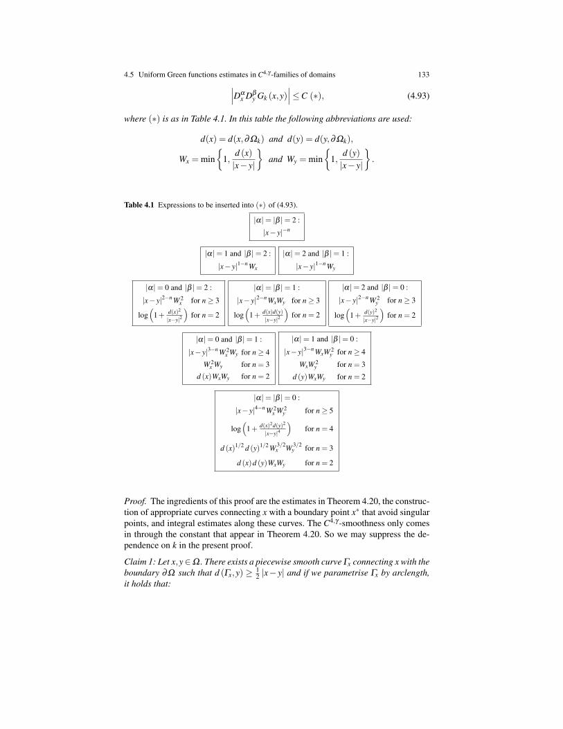
4.5 Uniform Green functions estimates in C4,γ -families of domains 133∣∣∣Dαx Dβ
y Gk (x,y)∣∣∣≤C (∗), (4.93)
where (∗) is as in Table 4.1. In this table the following abbreviations are used:
d(x) = d(x,∂Ωk) and d(y) = d(y,∂Ωk),
Wx = min
1,d (x)|x− y|
and Wy = min
1,
d (y)|x− y|
.
Table 4.1 Expressions to be inserted into (∗) of (4.93).
|α|= |β |= 2 :
|x− y|−n
|α|= 1 and |β |= 2 :
|x− y|1−n Wx
|α|= 2 and |β |= 1 :
|x− y|1−n Wy
|α|= 0 and |β |= 2 :
|x− y|2−n W 2x for n≥ 3
log(
1+ d(x)2
|x−y|2
)for n = 2
|α|= |β |= 1 :
|x− y|2−n WxWy for n≥ 3
log(
1+ d(x)d(y)|x−y|2
)for n = 2
|α|= 2 and |β |= 0 :
|x− y|2−n W 2y for n≥ 3
log(
1+ d(y)2
|x−y|2
)for n = 2
|α|= 0 and |β |= 1 :
|x− y|3−n W 2x Wy for n≥ 4
W 2x Wy for n = 3
d (x)WxWy for n = 2
|α|= 1 and |β |= 0 :
|x− y|3−n WxW 2y for n≥ 4
WxW 2y for n = 3
d (y)WxWy for n = 2
|α|= |β |= 0 :
|x− y|4−n W 2x W 2
y for n≥ 5
log(
1+ d(x)2d(y)2
|x−y|4
)for n = 4
d (x)1/2 d (y)1/2 W 3/2x W 3/2
y for n = 3
d (x)d (y)WxWy for n = 2
Proof. The ingredients of this proof are the estimates in Theorem 4.20, the construc-tion of appropriate curves connecting x with a boundary point x∗ that avoid singularpoints, and integral estimates along these curves. The C4,γ -smoothness only comesin through the constant that appear in Theorem 4.20. So we may suppress the de-pendence on k in the present proof.
Claim 1: Let x,y∈Ω . There exists a piecewise smooth curve Γx connecting x with theboundary ∂Ω such that d (Γx,y) ≥ 1
2 |x− y| and if we parametrise Γx by arclength,it holds that:
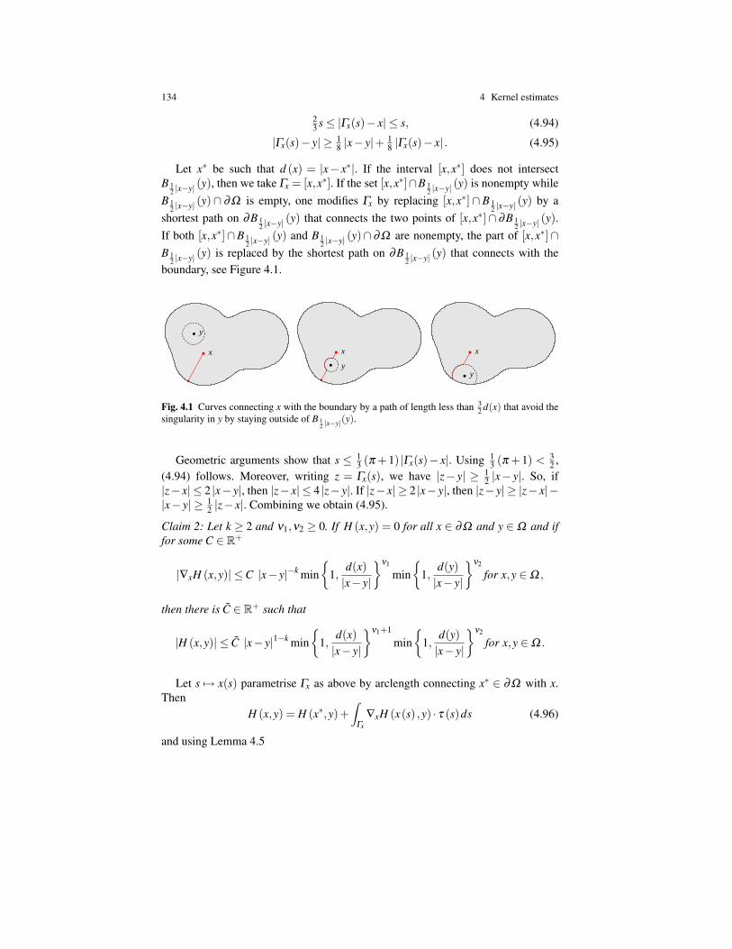
134 4 Kernel estimates
23 s≤ |Γx(s)− x| ≤ s, (4.94)
|Γx(s)− y| ≥ 18 |x− y|+ 1
8 |Γx(s)− x| . (4.95)
Let x∗ be such that d (x) = |x− x∗|. If the interval [x,x∗] does not intersectB 1
2 |x−y| (y), then we take Γx = [x,x∗]. If the set [x,x∗]∩B 12 |x−y| (y) is nonempty while
B 12 |x−y| (y)∩ ∂Ω is empty, one modifies Γx by replacing [x,x∗]∩ B 1
2 |x−y| (y) by ashortest path on ∂B 1
2 |x−y| (y) that connects the two points of [x,x∗]∩ ∂B 12 |x−y| (y).
If both [x,x∗]∩B 12 |x−y| (y) and B 1
2 |x−y| (y)∩ ∂Ω are nonempty, the part of [x,x∗]∩B 1
2 |x−y| (y) is replaced by the shortest path on ∂B 12 |x−y| (y) that connects with the
boundary, see Figure 4.1.
x
y
x
y
x
y
Fig. 4.1 Curves connecting x with the boundary by a path of length less than 32 d(x) that avoid the
singularity in y by staying outside of B 12 |x−y|(y).
Geometric arguments show that s ≤ 13 (π +1) |Γx(s)− x|. Using 1
3 (π +1) < 32 ,
(4.94) follows. Moreover, writing z = Γx(s), we have |z− y| ≥ 12 |x− y|. So, if
|z− x| ≤ 2 |x− y|, then |z− x| ≤ 4 |z− y|. If |z− x| ≥ 2 |x− y|, then |z− y| ≥ |z− x|−|x− y| ≥ 1
2 |z− x|. Combining we obtain (4.95).
Claim 2: Let k ≥ 2 and ν1,ν2 ≥ 0. If H (x,y) = 0 for all x ∈ ∂Ω and y ∈ Ω and iffor some C ∈ R+
|∇xH (x,y)| ≤C |x− y|−k min
1,d(x)|x− y|
ν1
min
1,d(y)|x− y|
ν2
for x,y ∈Ω ,
then there is C ∈ R+ such that
|H (x,y)| ≤ C |x− y|1−k min
1,d(x)|x− y|
ν1+1
min
1,d(y)|x− y|
ν2
for x,y ∈Ω .
Let s 7→ x(s) parametrise Γx as above by arclength connecting x∗ ∈ ∂Ω with x.Then
H (x,y) = H (x∗,y)+∫
Γx
∇xH (x(s) ,y) · τ (s)ds (4.96)
and using Lemma 4.5
4.5 Uniform Green functions estimates in C4,γ -families of domains 135
|H (x,y)| ≤∫
Γx
|∇xH (x(s) ,y)|ds
≤∫
Γx
C |x(s)− y|−k min
1,d(x(s))ν1d(y)ν2
|x(s)− y|ν1+ν2
ds.
It follows from (4.95) that
|H (x,y)| ≤ c1
∫ 32 d(x)
0(|x− y|+ s)−k min
1,
d(x)ν1d(y)ν2
(|x− y|+ s)ν1+ν2
ds
= c1 |x− y|1−k∫ 3
2d(x)|x−y|
0(1+ t)−k min
1,
d(x)ν1d(y)ν2
(1+ t)ν1+ν2 |x− y|ν1+ν2
dt.
We distinguish two cases. If d(x)≤ |x− y|, then
|H (x,y)| ≤ c1 |x− y|1−k∫ 3
2d(x)|x−y|
0min
1,
d(x)ν1d(y)ν2
|x− y|ν1+ν2
dt
≤ c2 |x− y|1−k min
1,d(x)ν1d(y)ν2
|x− y|ν1+ν2
d(x)|x− y|
≤ c3 |x− y|1−k min
1,
d(x)ν1+1d(y)ν2
|x− y|ν1+ν2+1
. (4.97)
If d(x)≥ |x− y|, then
|H (x,y)| ≤ c1 |x− y|1−k∫ 3
2d(x)|x−y|
0(1+ t)−k dt · min
1,
d(y)ν2
|x− y|ν2
≤ c2 |x− y|1−k min
1,
d(y)ν2
|x− y|ν2
≤ c3 |x− y|1−k min
1,
d(x)ν1+1d(y)ν2
|x− y|ν1+ν2+1
.
Claim 3: Let ν1,ν2 ≥ 0. If H (x,y) = 0 for x ∈ ∂Ω and for some C ∈ R+
|∇xH (x,y)| ≤C |x− y|−1 min
1,d(x)|x− y|
ν1
min
1,d(y)|x− y|
ν2
for x,y ∈Ω ,
then there is C ∈ R+ such that for all x,y ∈Ω
|H (x,y)| ≤ C log(
2+d(x)|x− y|
)min
1,
d(x)|x− y|
ν1+1
min
1,d(y)|x− y|
ν2
.
The steps of Claim 2 remain valid until
136 4 Kernel estimates
|H (x,y)| ≤ c1
∫ 32
d(x)|x−y|
0(1+ t)−1 min
1,
d(x)ν1d(y)ν2
(1+ t)ν1+ν2 |x− y|ν1+ν2
dt,
and inclusive (4.97). For d(x)≤ |x− y| the claim follows. If d(x)≥ |x− y|, then
∫ 32
d(x)|x−y|
0(1+ t)−1 min
1,
d(x)ν1d(y)ν2
(1+ t)ν1+ν2 |x− y|ν1+ν2
dt
≤ log(
2+d(x)|x− y|
)min
1,
d(x)ν1d(y)ν2
|x− y|ν1+ν2
≤ log
(2+
d(x)|x− y|
)min
1,
d(x)ν1+1d(y)ν2
|x− y|ν1+ν2+1
.
Claim 4: Let k ≥ 2 and ν1,ν2,α1,α2 ≥ 0. If H (x,y) = 0 for x ∈ ∂Ω and for someC ∈ R+
|∇xH (x,y)| ≤C d(x)α1d(y)α2 min
1,d(x)|x− y|
ν1
min
1,d(y)|x− y|
ν2
for x,y ∈Ω ,
then there is C ∈ R+ such that
|H (x,y)| ≤ C d(x)α1+1d(y)α2 min
1,d(x)|x− y|
ν1
min
1,d(y)|x− y|
ν2
for x,y ∈Ω .
This is a direct consequence of (4.96), (4.94) and (4.95).
Claim 5: Let k ≥ 2 and ν1,ν2,α1,α2 ≥ 0. If H (x,y) = 0 for x ∈ ∂Ω and if thereexists C ∈ R+ such that
|∇xH (x,y)| ≤C log
(2+
d(x)d(y)|x− y|2
)min
1,
d(x)|x− y|
ν1
min
1,d(y)|x− y|
ν2
for x,y ∈Ω , then there is C ∈ R+ such that
|H (x,y)| ≤ C d(x)min
1,d(x)|x− y|
ν1
min
1,d(y)|x− y|
ν2
for x,y ∈Ω .
We first observe that
log
(2+
d(x)d(y)|x− y|2
)min
1,
d(x)|x− y|
ν1
min
1,d(y)|x− y|
ν2
' log(
2+d(x)|x− y|
)min
1,
d(x)|x− y|
ν1
min
1,d(y)|x− y|
ν2
4.5 Uniform Green functions estimates in C4,γ -families of domains 137
If d(x)|x−y| ≤ 1, then log
(2+ d(x)
|x−y|
)is bounded and the result is again a direct conse-
quence of (4.96), (4.94) and (4.95). If d(x)|x−y| ≥ 1, then for z ∈ Γx
d(z)|x− z|
≤ 8d(z)|x− y|+ s
and one finds
|∇xH (x(s),y)| ≤ c1 log(
2+d(x)
|x− y|+ s
)· min
1,
d(y)ν2
|x− y|ν2
.
Hence
|H (x,y)| ≤ c1
∫ 32 d(x)
0log(
2+d(x)
|x− y|+ s
)ds · min
1,
d(y)ν2
|x− y|ν2
≤ c2d(x)min
1,
d(y)ν2
|x− y|ν2
.
In order to complete the proof of Theorem 4.28 one starts from the estimates ofTheorem 4.20. We find, using the Claims 2 to 5 and working our way down, theestimates as in Table 4.1 except for n = 3 with |α|+ |β | ≤ 1. Suppose α = 0 and|β |= 1. Then∣∣∣∇xDβ
y G(x,y)∣∣∣≤C |x− y|−1 min
1,
d(x)|x− y|
min
1,
d(y)|x− y|
implies ∣∣∣Dβ
y G(x,y)∣∣∣≤C log
(1+
d(x)2d(y)|x− y|3
).
Together with (4.76) we obtain∣∣∣Dβy G(x,y)
∣∣∣≤C min
1,d(x)|x− y|
2
min
1,d(y)|x− y|
.
For the zeroth order in case n = 3 one finds through
∣∣∇yG(x,y)∣∣≤C min
1,
d(x)|x− y|
2
min
1,d(y)|x− y|
that
|G(x,y)| ≤C d(y)min
1,d(x)|x− y|
2
min
1,d(y)|x− y|
and through the similar estimate for |∇xG(x,y)| that
138 4 Kernel estimates
|G(x,y)| ≤C M (x,y)min
1,
d(x)d(y)|x− y|2
with
M (x,y) = min
d(y)min
1,d(x)|x− y|
,d(x)min
1,
d(y)|x− y|
.
Since M (x,y)≤√
d(x)d(y)min
1, d(x)d(y)|x−y|2
3/2the proof is complete.
In a similar way one may derive estimates for the Poisson kernels. Consider∆ 2u = f in Ω ,
u|∂Ω = ψ, − ∂u∂ν|∂Ω = ϕ.
(4.98)
If G = G∆ 2,Ω is the Green function for this boundary value problem, then the solu-tion of (4.98) is written as
u(x) =∫
Ω
G(x,y) f (y) dy+∫
∂Ω
K (x,y)ψ(y) dωy +∫
∂Ω
L(x,y)ϕ(y) dωy,
with K,L : Ω ×∂Ω → R defined by
K (x,y) =∂
∂νy∆yG(x,y),
L(x,y) = ∆yG(x,y).
Theorem 4.29. Let (Ωk)k∈N be as in Theorem 4.28 and let KΩk and LΩk be thecorresponding Poisson kernels. Then there exists C = C
((Ωk)k∈N
)such that for all
(x,y) ∈Ω ×∂Ω :
∣∣KΩk (x,y)∣∣≤C
d (x)2
|x− y|n+1 and∣∣LΩk (x,y)
∣∣≤Cd (x)2
|x− y|n.
For n = 2 one obtains∣∣LΩk (x,y)
∣∣≤C.
4.5.3 Convergence of the Green function in domainapproximations
Proposition 4.30. Let xk ∈Ωk and assume that limk→∞ xk = x∞ ∈Ω . Then we have
Gk(xk, .) → G(x∞, .) in C4loc(Ω \x∞),
Gk(xk, .) → G(x∞, .) in L1(Rn),Gk(xk, .)Ψk → G(x∞, .) in C4
loc(Ω \x∞).
4.6 Weighted estimates for the Dirichlet problem 139
If n = 3 we have in addition that
Gk( . , .)→ G( . , .) in C0loc(Ω ×Ω).
Proof. According to Theorem 4.20 we know that
|Gk(x,y)| ≤C
|x− y|4−n if n > 4,log(1+ |x− y|−1
)if n = 4,
1 if n = 3;(4.99)
uniformly in k. This shows that in particular
‖Gk(x, .)‖L1(Ωk) ≤C uniformly in x and k.
Moreover, since xk → x∞, we may assume that all xk are in a small neighbour-hood around x∞. Let Ω0 ⊂⊂ Ω be arbitrary; local Schauder estimates (see Theo-rem 2.19) show that (Gk(xk, .))k∈N is locally bounded in C4
loc
(Ω0 \x∞
). Hence,
after selecting a suitable subsequence we see that for each such Ω0 ⊂⊂ Ω one hasGk(xk, .)→ ϕ in C4
loc
(Ω0 \x∞
)and Gk(xk, .)Ψk → ϕ in C4
loc(Ω \x∞) with asuitable ϕ ∈ C4,γ(Ω \ x∞). Thanks to this compactness and the fact that in anycase the limit is the uniquely determined Green function, we have convergence onthe whole sequence towards G(x∞, .).
Finally, since we have pointwise convergence, (4.99) allows for applying Vitali’sconvergence theorem to show that
Gk(xk, .)→ G(x∞, .) in L1(Rn).
The statement concerning C0loc(Ω ×Ω)-convergence in n = 3 is a consequence of
|∇Gk( . , .)| ≤C, see (4.60).
In order to have enough smoothness to conclude also for the last case in Theo-rem 6.30 we also need a convergence result simultaneous in both variables.
Proposition 4.31. We have that
Gk( . , .) (Ψk×Ψk)→ G( . , .) in C4loc(Ω ×Ω \(x,x) ;x ∈Ω
).
Proof. We combine the ideas of the proofs of Propositions 4.30 and 4.17. Oneshould observe that Theorem 4.20 guarantees uniform L1-bounds for Gk as in theproof of Proposition 4.30.
4.6 Weighted estimates for the Dirichlet problem
As a side result the estimates in the previous section for the homogeneous bihar-monic Dirichlet problem allow weighted Lp-Lq estimates for elliptic boundary valueproblems under homogeneous boundary conditions with d ( .)θ as weight function.
140 4 Kernel estimates
Here we will restrict ourselves to the biharmonic case. A more general version ofthis theorem is found in [118].
If u and f are such that ∆ 2u = f in Ω ,u = uν = 0 on ∂Ω ,
(4.100)
then we have
Theorem 4.32. Let Ω be a bounded C4,γ -smooth domain and let u ∈ C4(Ω), f ∈
C(Ω)
be as in (4.100). Then the following hold:
1. For n < 4 there exists C = C (Ω) such that for all θ ∈ [0,1]:∥∥∥d ( .)θn−2 u∥∥∥
L∞(Ω)≤C
∥∥∥d( .)2−(1−θ)n f∥∥∥
L1(Ω). (4.101)
2. For all n≥ 2 if p,q∈ [1,∞] are such that 0≤ 1p −
1q < α ≤min
1, 4
n
, then there
exists C = C (Ω ,α) such that for all θ ∈ [0,1]:∥∥∥d ( .)θnα−2 u∥∥∥
Lq(Ω)≤C
∥∥∥d( .)2−(1−θ)nα f∥∥∥
Lp(Ω). (4.102)
Remark 4.33. Notice that the shift in the exponent of d ( .) in (4.102) is 4−nα withα > 0. If p = q this shift can be arbitrarily close to 4 but will not reach 4.
Before proving this theorem we recall an estimate involving the Riesz potential(Kγ ∗ f
)(x) :=
∫Ω
|x− y|−γ f (y)dy.
We prove a classical convolution estimate which can e.g. be found in [231, Corol-lary 4.5.2].
Lemma 4.34. Let Ω ⊂ Rn be bounded, γ ∈ (0,n) and 1 ≤ p,q ≤ ∞. If γ
n < 1r :=
min
1,1+ 1q −
1p
, then there exists C = C (diam(Ω),n− γr) ∈ R+ such that for
all f ∈ Lp(Ω): ∥∥Kγ ∗ f∥∥
Lq(Ω) ≤C ‖ f‖Lp(Ω) . (4.103)
Proof. We let p′ ∈ [1,∞] denote the conjugate of p ∈ [1,∞]: 1p + 1
p′ = 1 etc. Set
CΩ ,s = maxx∈Ω
∥∥|x− . |−s∥∥L1(Ω)
and notice that CΩ ,s is bounded for s < n.If q = 1, then r = 1 and a change in the order of integration gives
∥∥Kγ ∗ f∥∥
L1(Ω) ≤∫
Ω
(∫Ω
|x− y|−γ dx)| f (y)|dy
≤CΩ ,γr ‖ f‖L1(Ω) ≤C ‖ f‖Lp(Ω) . (4.104)
4.6 Weighted estimates for the Dirichlet problem 141
If p≥ q, then r = 1 and
∥∥Kγ ∗ f∥∥q
Lq(Ω) =∫
Ω
∣∣∣∣∫Ω
|x− y|−γ f (y)dy∣∣∣∣q dx
≤∫
Ω
(∫Ω
|x− y|−γ dy) q
q′(∫
Ω
|x− y|−γ | f (y)|q dx)
dy
≤ Cq/q′
Ω ,γr
∥∥Kγ ∗ | f |q∥∥
L1(Ω)
and one continues with (4.104).One finds for 1 < p < q < ∞, since 1
r′ +1p′ +
1q = 1, that∣∣(Kγ ∗ f
)(x)∣∣ ≤
≤(∫
Ω
| f (y)|p dy) 1
r′(∫
Ω
|x− y|−rγ dy) 1
p′(∫
Ω
|x− y|−rγ | f (y)|p dy) 1
q
(4.105)
and, by changing the order of integration and using pq/r′+ p = q, also
∥∥Kγ ∗ f∥∥q
Lq(Ω) ≤ ‖ f‖pq/r′
Lp(Ω)Cq/p′
Ω ,γr
∫Ω
(∫Ω
|x− y|−rγ dx)| f (y)|p dy
≤ C1+q/p′
Ω ,γr ‖ f‖qLp(Ω) . (4.106)
For q = ∞ and has r = p′ and the proof reduces to∣∣(Kγ ∗ f)(x)∣∣≤ ∥∥|x− . |−γ
∥∥Lp′ (Ω) ‖ f‖Lp(Ω) ≤C1/r
Ω ,γr ‖ f‖Lp(Ω) .
For p = 1 one replaces (4.105) by
∣∣(Kγ ∗ f)(x)∣∣≤ (∫
Ω
| f (y)|dy) 1
q′(∫
Ω
|x− y|−qγ | f (y)|dy) 1
q
and continues similar as in (4.106) by changing the order of integration.
Proof of Theorem 4.32. Again we use the notation (4.1). The estimate that we willuse repeatedly is a consequence of Lemma 4.5:
min
1,
d (x)d (y)|x− y|2
≤C
(d (x)d (y)|x− y|2
)1−s(d (y)d (x)
)s(2θ−1)
for all s,θ ∈ [0,1] .
(4.107)To prove Item 1 in Theorem 4.32 we apply this estimate for s = 1 to find for n < 4
|G(x,y)| ≤Cd(x)2− 12 nd(y)2− 1
2 n(
d (y)d (x)
) 12 n(2θ−1)
= Cd(x)2−nθ d(y)2−n(1−θ)
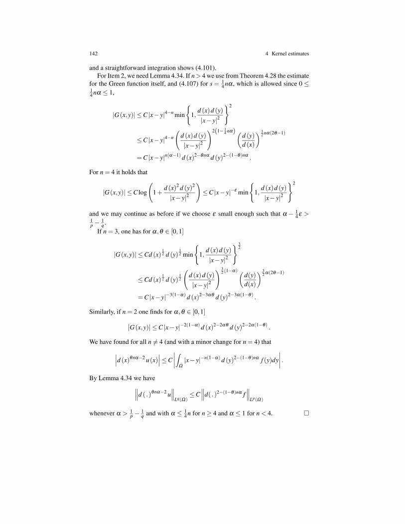
142 4 Kernel estimates
and a straightforward integration shows (4.101).For Item 2, we need Lemma 4.34. If n > 4 we use from Theorem 4.28 the estimate
for the Green function itself, and (4.107) for s = 14 nα , which is allowed since 0 ≤
14 nα ≤ 1,
|G(x,y)| ≤C |x− y|4−n min
1,
d (x)d (y)|x− y|2
2
≤C |x− y|4−n
(d (x)d (y)|x− y|2
)2(1− 14 nα)(
d (y)d (x)
) 12 nα(2θ−1)
= C |x− y|n(α−1) d (x)2−θnα d (y)2−(1−θ)nα .
For n = 4 it holds that
|G(x,y)| ≤C log
(1+
d (x)2 d (y)2
|x− y|2
)≤C |x− y|−ε min
1,
d (x)d (y)|x− y|2
2
and we may continue as before if we choose ε small enough such that α − 14 ε >
1p −
1q .
If n = 3, one has for α,θ ∈ [0,1]
|G(x,y)| ≤Cd (x)12 d (y)
12 min
1,
d (x)d (y)|x− y|2
32
≤Cd (x)12 d (y)
12
(d (x)d (y)|x− y|2
) 32 (1−α)(
d(y)d(x)
) 32 α(2θ−1)
= C |x− y|−3(1−α) d (x)2−3αθ d (y)2−3α(1−θ) .
Similarly, if n = 2 one finds for α,θ ∈ [0,1]
|G(x,y)| ≤C |x− y|−2(1−α) d (x)2−2αθ d (y)2−2α(1−θ) .
We have found for all n 6= 4 (and with a minor change for n = 4) that∣∣∣d (x)θnα−2 u(x)∣∣∣≤C
∣∣∣∣∫Ω
|x− y|−n(1−α) d (y)2−(1−θ)nα f (y)dy∣∣∣∣ .
By Lemma 4.34 we have∥∥∥d ( .)θnα−2 u∥∥∥
Lq(Ω)≤C
∥∥∥d( .)2−(1−θ)nα f∥∥∥
Lp(Ω)
whenever α > 1p −
1q and with α ≤ 1
4 n for n≥ 4 and α ≤ 1 for n < 4.
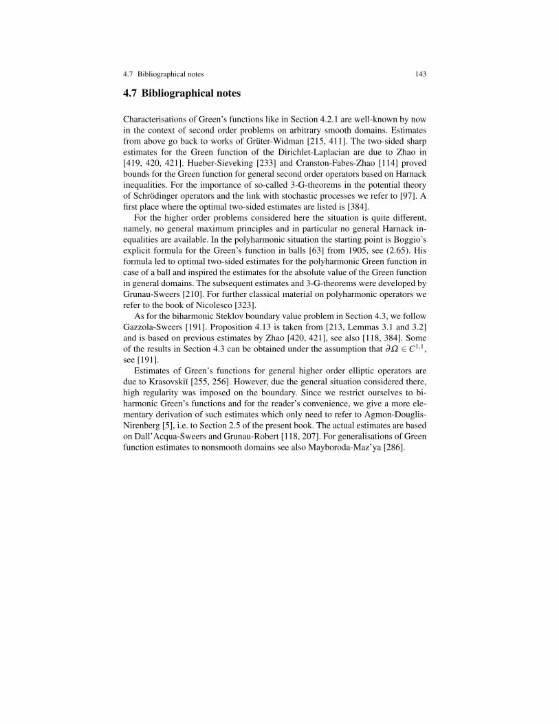
4.7 Bibliographical notes 143
4.7 Bibliographical notes
Characterisations of Green’s functions like in Section 4.2.1 are well-known by nowin the context of second order problems on arbitrary smooth domains. Estimatesfrom above go back to works of Gruter-Widman [215, 411]. The two-sided sharpestimates for the Green function of the Dirichlet-Laplacian are due to Zhao in[419, 420, 421]. Hueber-Sieveking [233] and Cranston-Fabes-Zhao [114] provedbounds for the Green function for general second order operators based on Harnackinequalities. For the importance of so-called 3-G-theorems in the potential theoryof Schrodinger operators and the link with stochastic processes we refer to [97]. Afirst place where the optimal two-sided estimates are listed is [384].
For the higher order problems considered here the situation is quite different,namely, no general maximum principles and in particular no general Harnack in-equalities are available. In the polyharmonic situation the starting point is Boggio’sexplicit formula for the Green’s function in balls [63] from 1905, see (2.65). Hisformula led to optimal two-sided estimates for the polyharmonic Green function incase of a ball and inspired the estimates for the absolute value of the Green functionin general domains. The subsequent estimates and 3-G-theorems were developed byGrunau-Sweers [210]. For further classical material on polyharmonic operators werefer to the book of Nicolesco [323].
As for the biharmonic Steklov boundary value problem in Section 4.3, we followGazzola-Sweers [191]. Proposition 4.13 is taken from [213, Lemmas 3.1 and 3.2]and is based on previous estimates by Zhao [420, 421], see also [118, 384]. Someof the results in Section 4.3 can be obtained under the assumption that ∂Ω ∈C1,1,see [191].
Estimates of Green’s functions for general higher order elliptic operators aredue to Krasovskiı [255, 256]. However, due the general situation considered there,high regularity was imposed on the boundary. Since we restrict ourselves to bi-harmonic Green’s functions and for the reader’s convenience, we give a more ele-mentary derivation of such estimates which only need to refer to Agmon-Douglis-Nirenberg [5], i.e. to Section 2.5 of the present book. The actual estimates are basedon Dall’Acqua-Sweers and Grunau-Robert [118, 207]. For generalisations of Greenfunction estimates to nonsmooth domains see also Mayboroda-Maz’ya [286].

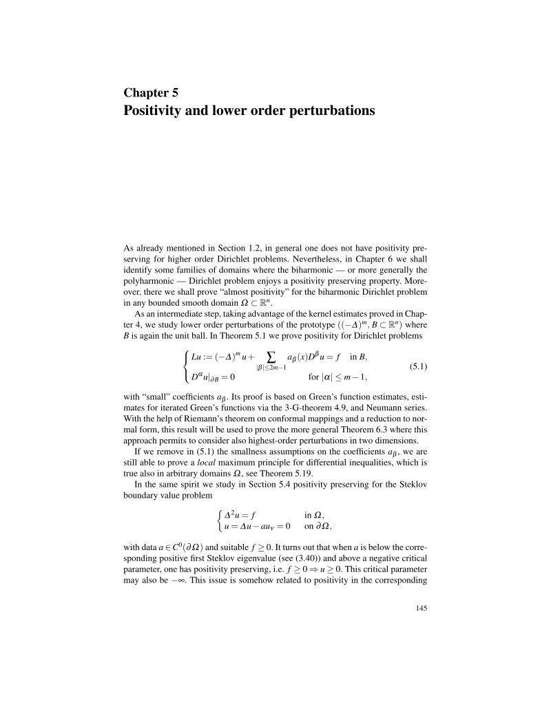
Chapter 5Positivity and lower order perturbations
As already mentioned in Section 1.2, in general one does not have positivity pre-serving for higher order Dirichlet problems. Nevertheless, in Chapter 6 we shallidentify some families of domains where the biharmonic — or more generally thepolyharmonic — Dirichlet problem enjoys a positivity preserving property. More-over, there we shall prove “almost positivity” for the biharmonic Dirichlet problemin any bounded smooth domain Ω ⊂ Rn.
As an intermediate step, taking advantage of the kernel estimates proved in Chap-ter 4, we study lower order perturbations of the prototype ((−∆)m, B⊂ Rn) whereB is again the unit ball. In Theorem 5.1 we prove positivity for Dirichlet problemsLu := (−∆)m u+ ∑
|β |≤2m−1aβ (x)Dβ u = f in B,
Dα u|∂B = 0 for |α| ≤ m−1,(5.1)
with “small” coefficients aβ . Its proof is based on Green’s function estimates, esti-mates for iterated Green’s functions via the 3-G-theorem 4.9, and Neumann series.With the help of Riemann’s theorem on conformal mappings and a reduction to nor-mal form, this result will be used to prove the more general Theorem 6.3 where thisapproach permits to consider also highest-order perturbations in two dimensions.
If we remove in (5.1) the smallness assumptions on the coefficients aβ , we arestill able to prove a local maximum principle for differential inequalities, which istrue also in arbitrary domains Ω , see Theorem 5.19.
In the same spirit we study in Section 5.4 positivity preserving for the Steklovboundary value problem
∆ 2u = f in Ω ,u = ∆u−auν = 0 on ∂Ω ,
with data a∈C0(∂Ω) and suitable f ≥ 0. It turns out that when a is below the corre-sponding positive first Steklov eigenvalue (see (3.40)) and above a negative criticalparameter, one has positivity preserving, i.e. f ≥ 0⇒ u≥ 0. This critical parametermay also be −∞. This issue is somehow related to positivity in the corresponding
145
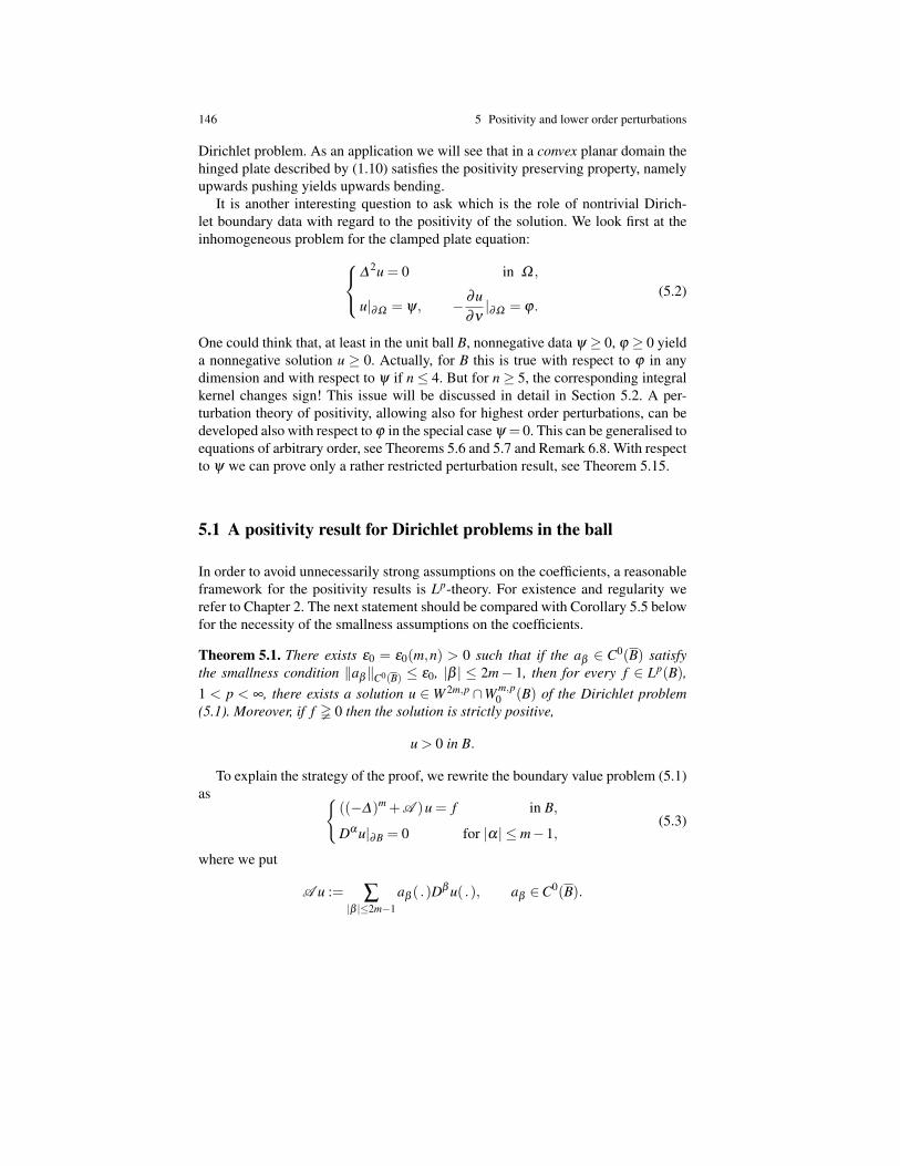
146 5 Positivity and lower order perturbations
Dirichlet problem. As an application we will see that in a convex planar domain thehinged plate described by (1.10) satisfies the positivity preserving property, namelyupwards pushing yields upwards bending.
It is another interesting question to ask which is the role of nontrivial Dirich-let boundary data with regard to the positivity of the solution. We look first at theinhomogeneous problem for the clamped plate equation:
∆2u = 0 in Ω ,
u|∂Ω = ψ, − ∂u∂ν|∂Ω = ϕ.
(5.2)
One could think that, at least in the unit ball B, nonnegative data ψ ≥ 0, ϕ ≥ 0 yielda nonnegative solution u ≥ 0. Actually, for B this is true with respect to ϕ in anydimension and with respect to ψ if n≤ 4. But for n≥ 5, the corresponding integralkernel changes sign! This issue will be discussed in detail in Section 5.2. A per-turbation theory of positivity, allowing also for highest order perturbations, can bedeveloped also with respect to ϕ in the special case ψ = 0. This can be generalised toequations of arbitrary order, see Theorems 5.6 and 5.7 and Remark 6.8. With respectto ψ we can prove only a rather restricted perturbation result, see Theorem 5.15.
5.1 A positivity result for Dirichlet problems in the ball
In order to avoid unnecessarily strong assumptions on the coefficients, a reasonableframework for the positivity results is Lp-theory. For existence and regularity werefer to Chapter 2. The next statement should be compared with Corollary 5.5 belowfor the necessity of the smallness assumptions on the coefficients.
Theorem 5.1. There exists ε0 = ε0(m,n) > 0 such that if the aβ ∈ C0(B) satisfythe smallness condition ‖aβ‖C0(B) ≤ ε0, |β | ≤ 2m− 1, then for every f ∈ Lp(B),1 < p < ∞, there exists a solution u ∈W 2m,p ∩W m,p
0 (B) of the Dirichlet problem(5.1). Moreover, if f 0 then the solution is strictly positive,
u > 0 in B.
To explain the strategy of the proof, we rewrite the boundary value problem (5.1)as
((−∆)m +A )u = f in B,
Dα u|∂B = 0 for |α| ≤ m−1,(5.3)
where we put
A u := ∑|β |≤2m−1
aβ ( .)Dβ u( .), aβ ∈C0(B).
5.1 A positivity result for Dirichlet problems in the ball 147
We recall from Section 4.2.1 the definition of the Green operator Gm,n for the bound-ary value problem (5.3) with A = 0. In order to prove Theorem 5.1, we write thesolution of (5.3) in the form
u = (I +Gm,nA )−1 Gm,n f ,
where I is the identity operator, and we shall estimate
(I +Gm,nA )−1 Gm,n ≥1C
Gm,n.
For this purpose we introduce the following notation.
Definition 5.2. For two operators S ,T : Lp(B)→ Lp(B) we write
S ≥T ,
if for all f ∈ Lp(B) satisfying f ≥ 0, one has that S f ≥T f .
Lemma 5.3. Let 1 < p < ∞. Then Gm,nA : W 2m,p ∩W m,p0 (B) →W 2m,p ∩W m,p
0 (B)is a bounded linear operator. Furthermore, there exists ε1 = ε1(m,n) > 0 such thatthe following holds true.
Assume that ‖aβ‖C0(B) ≤ ε1 for all |β | ≤ 2m− 1. Then I + Gm,nA : W 2m,p ∩W m,p
0 (B) → W 2m,p ∩W m,p0 (B) is boundedly invertible. For each f ∈ Lp(B) the
boundary value problem (5.3) has precisely one solution. This solution is given by
u = (I +Gm,nA )−1 Gm,n f . (5.4)
The Green operator for the boundary value problem (5.3)
(I +Gm,nA )−1 Gm,n : Lp(B)→W 2m,p∩W m,p0 (B)⊂ Lp(B)
is compact.
Proof. This is an immediate consequence of Corollary 2.21: Gm,n : Lp(B)→W 2m,p∩W m,p
0 (B) is a bounded linear operator.
The Green operator for (5.3) is studied with the help of a Neumann series. The-orem 5.1 then follows from the next result.
Theorem 5.4. Assume that 1 < p < ∞. There exists ε0 = ε0(m,n) > 0 such that if‖aβ‖C0(B) ≤ ε0 for all |β | ≤ 2m−1, then the Green operator
Gm,n,A := (I +Gm,nA )−1 Gm,n : Lp(B)→W 2m,p∩W m,p0 (B)
for the boundary value problem (5.3) exists. The corresponding Green functionGm,n,A : B×B→ R∪∞ is defined according to:(
Gm,n,A f)(x) =
∫B
Gm,n,A (x,y) f (y)dy

148 5 Positivity and lower order perturbations
and satisfies the following estimate with a constant C = C(m,n) > 0:
1C
Gm,n ≤ Gm,n,A ≤CGm,n. (5.5)
On B×B, this reads:
1C
Gm,n(x,y)≤ Gm,n,A (x,y)≤C Gm,n(x,y). (5.6)
Proof. Let ε := max|β |≤2m−1 ‖aβ‖C0(B). If ε ≤ ε1, then according to Lemma 5.3,Gm,n,A exists and enjoys the properties listed there. If we choose moreover ε smallenough such that ‖Gm,nA ‖< 1 in the sense of bounded linear operators in W 2m,p∩W m,p
0 (B), we may use a Neumann series to see that for all f ∈ Lp(B)
Gm,n,A f = (I +Gm,nA )−1 Gm,n f =∞
∑i=0
(−1)i (Gm,nA )i Gm,n f .
Here, with the aid of the Fubini-Tonelli theorem and analogously to [197, Lemma4.1], we conclude:
G (i) f := (−1)i (Gm,nA )i Gm,n f
= (−1)i∫
BGm,n( . ,z1)Az1
∫B
Gm,n(z1,z2)Az2 . . .
. . .Azi
∫B
Gm,n(zi,y) f (y)dydzi . . .dz1
=∫
B
(−1)i
∫B· · ·∫
BGm,n( . ,z1)(Az1Gm,n(z1,z2)) . . .
. . .(AziGm,n(zi,y)) d(z1, . . . ,zi)
f (y)dy
=:∫
BG(i)( . ,y) f (y)dy.
We use the following version of the 3-G-theorem 4.9:∫B
Gm,n(x,z) |AzGm,n(z,y)|Gm,n(x,y)
dz≤ εM < ∞
where M = M(m,n) > 0 is independent of ε and obtain:∣∣∣G(i)(x,y)∣∣∣ =
=∣∣∣∣∫B
· · ·∫
B
Gm,n(x,z1)(Az1Gm,n(z1,z2))Gm,n(x,z2)
Gm,n(x,z2)(Az2Gm,n(z2,z3))Gm,n(x,z3)
· · ·
· · ·Gm,n(x,zi)(AziGm,n(zi,y))
Gm,n(x,y)Gm,n(x,y)d(z1, . . . ,zi)
∣∣∣∣ ≤
5.1 A positivity result for Dirichlet problems in the ball 149
≤ Gm,n(x,y)i
∏j=1
supξ ,η∈B
∫B
Gm,n(ξ ,z j)∣∣Az j Gm,n(z j,η)
∣∣Gm,n(ξ ,η)
dz j
≤ (εM)i Gm,n(x,y). (5.7)
For εM < 1, thanks to ∑∞i=0(εM)i = (1− εM)−1 < ∞, we have absolute local uni-
form convergence in x 6= y of
Gm,n,A (x,y) :=∞
∑i=0
G(i)(x,y). (5.8)
It follows that ∣∣Gm,n,A (x,y)∣∣≤ 1
1− εMGm,n(x,y). (5.9)
On the other hand, Lebesgue’s theorem yields
(Gm,n,A f
)(x) =
∞
∑i=0
(G (i) f
)(x) =
∞
∑i=0
∫B
G(i)(x,y) f (y)dy
=∫
B
(∞
∑i=0
G(i)(x,y) f (y)
)dy =
∫B
Gm,n,A (x,y) f (y)dy.
Finally, thanks to (5.7) we have
Gm,n,A (x,y) = Gm,n(x,y)+∞
∑i=1
G(i)(x,y)
≥ Gm,n(x,y)−
(∞
∑i=1
(εM)i
)Gm,n(x,y) =
1−2εM1− εM
Gm,n(x,y).
Choosing ε0 ≤ 1/(4M) yields the crucial part of the estimate (5.6) from below forthe Green function of the perturbed boundary value problem (5.3), provided ε ∈[0,ε0].
If we confine ourselves to perturbations of order zero, we may show the necessityof the smallness conditions in Theorem 5.1. Consider the problem
(−∆)mu+a(x)u = f in Ω ,
Dα u|∂Ω = 0 for |α| ≤ m−1,(5.10)
where Ω ⊂ Rn is a bounded C2m,γ -smooth domain. For coefficients a ∈ C0(Ω),where we have uniqueness and hence existence in (5.10), let Gm,Ω ,a be the corre-sponding Green operator. In case of a constant coefficient a, Gm,Ω ,a is the resolventoperator. Recalling the meaning of the symbols
φ > 0 , φ 0 , φ 0 ,
150 5 Positivity and lower order perturbations
in the Notations-Section, the positivity properties of Dirichlet problem (5.10) maybe summarised as follows.
Corollary 5.5. Let m > 1 and let Ω ⊂ Rn be a bounded smooth domain such thatthe (Dirichlet-) Green function for (−∆)m is positive in Ω ×Ω . Let Λm,1 denote thefirst Dirichlet eigenvalue of (−∆)m in Ω .
Then there exists a critical number ac ∈ [0,∞) such that for a ∈C0(Ω) we have:
1. If a > ac on Ω , then Gm,Ω ,a does not preserve positivity:
there exists f 0 : Gm,Ω ,a f 6≥ 0. (5.11)
On the other hand we have:
for all f 0 : Gm,Ω ,a f 6≤ 0, (5.12)there exists f 0 : Gm,Ω ,a f ≥ 0. (5.13)
2. If −Λm,1 < a ≤ ac (or −Λm,1 < a < ac, respectively), then Gm,Ω ,a is positivitypreserving (or strongly positivity preserving, respectively), that is,
for all f 0 : Gm,Ω ,a f ≥ 0 (or Gm,Ω ,a f > 0 in Ω , respectively). (5.14)
3. If a =−Λm,1 and f 0, then (5.10) has no solution.4. If a < −Λm,1, then (5.10) kills positivity, that is, if f 0 and u is a solution to
(5.10), then u 6≥ 0 in Ω .
For a proof, the strategy of which is related to – but simpler than – the arguments inSection 5.4, we refer to [210, Section 6] and [212, Lemma 1].
Case 1 does not occur in second order equations. This different behaviour may beresponsible for the difficulties in classical solvability of semilinear boundary valueproblems of higher order, see e.g. [209, 395, 404, 405]. If m > 1, we have that for alarge enough the resolvent is always sign changing, see e.g. Coffman-Grover [111].As was noted e.g. by Bernis [51], this is equivalent to instantaneous change of signfor the corresponding parabolic heat kernel, see also related contributions to localeventual positivity by Ferrero-Gazzola-Grunau [164, 183, 184].
5.2 The role of positive boundary data
This section is devoted to the role of nonhomogeneous boundary data with regardto the sign of the solution. As already mentioned in the introduction this problem israther subtle. In general we cannot expect that fixed sign of any particular Dirich-let datum leads to fixed sign of the solution. It seems that a perturbation theoryof positivity (analogous to that above with regard to the right-hand side) exists in
5.2 The role of positive boundary data 151
general only for the Dirichlet datum of highest order. As a dual result we obtainalso a Hopf-type boundary lemma in the ball for perturbed polyharmonic Dirichletproblems.
With respect to lower order data, only much more restricted results can beachieved, see Theorem 5.15 below.
5.2.1 The highest order Dirichlet datum
Here, we consider the following boundary value problem:((−∆)m +A )u = f in B,
Dα u|∂B = 0 for |α| ≤ m−2,−∂
∂ν∆
(m/2)−1u|∂B = ϕ
∆(m−1)/2u|∂B = ϕ
if m is even,
if m is odd.
(5.15)
Here f ∈C0(B), ϕ ∈C0(∂B) and
A = ∑|β |≤2m−1
aβ ( .)Dβ , aβ ∈C|β |(B), (5.16)
is a sufficiently small lower order perturbation. For existence of solutions u ∈W 2m,p
loc (B)∩Cm−1(B), p > 1, we refer to the local Lp-theory in Theorem 2.20 and thelines following it and to the Agmon-Miranda maximum estimates of Theorem 2.25.The latter already require the strong regularity assumptions on the coefficients aβ .These have to be imposed whenever the adjoint operator (−∆)m +A ∗ is involved.
Theorem 5.6. There exists ε0 = ε0(m,n) > 0 such that the following holds true.If for all |β | ≤ 2m−1 the smallness condition ‖aβ‖C|β |(B)≤ ε0 is fulfilled, then for
every f ∈C0(B) and ϕ ∈C0(∂B) there exists a solution u ∈W 2m,ploc (B)∩Cm−1(B),
1 < p < ∞, to the Dirichlet problem (5.15). Moreover, f ≥ 0 and ϕ ≥ 0, with f 6≡ 0or ϕ 6≡ 0, implies that u > 0.
If m = 1, we recover a special form of the strong maximum principle for secondorder elliptic equations. The next result, in some sense dual to the previous one, maybe viewed as a higher order analogue to the Hopf boundary lemma.
Theorem 5.7. Assume aβ ∈ C0(B), |β | ≤ 2m− 1. There exists ε0 = ε0(m,n) > 0such that the following holds:
If ‖aβ‖C0(B) ≤ ε0, |β | ≤ 2m−1, then for every f ∈C0(B) the Dirichlet problem(5.1) has a solution u ∈W 2m,p(B)∩C2m−1(B), p > 1 arbitrary. Moreover 0 6≡ f ≥ 0implies u > 0 in B and for every x ∈ ∂B
152 5 Positivity and lower order perturbations∆
(m/2)u(x) > 0 if m even,
− ∂
∂ν∆
(m−1)/2u(x) > 0 if m odd.(5.17)
The common key point in the proof of both theorems is the observation that thecorresponding Green function Gm,n,A vanishes (in both variables) on ∂B preciselyof order m, see Theorem 4.7 and estimate (5.6). In the proof of Theorem 5.6 weobserve further that, for x ∈ B, y ∈ ∂B, the Poisson kernel for ϕ is given by
∆m/2y Gm,n,A (x,y) if m even,(− ∂
∂νy∆
(m−1)/2y
)Gm,n,A (x,y) if m odd.
In order to prove the theorems we need a precise characterisation of the growth prop-erties near ∂B of the Green function Gm,n,A for the boundary value problem (5.15).These estimates were proved in a more general setting but under more restrictiveassumptions on the coefficients by Krasovskiı [255, 256], see also Theorem 4.20.In the present special situation we provide an elementary proof which combinesTheorems 4.6 and 5.4. Moreover, we need to verify suitable smoothness.
Lemma 5.8. We assume that aβ ∈C0(B). Then there exists ε1 = ε1(m,n) > 0 suchthat the following holds true.
If ‖aβ‖C0(B) ≤ ε1 for all |β | ≤ 2m−1, then the Green function Gm,n,A ( . , .) forthe boundary value problem (5.15) exists. For each y ∈ B, Gm,n,A ( . ,y) ∈C2m−1(B\y). Furthermore, there exist constants C = C(m,n) such that for |β | ≤ 2m− 1,x,y ∈ B
Gm,n,A ( . ,y) ∈C|β |(B) if 0≤ |β |< 2m−n,∣∣∣Dβx Gm,n,A (x,y)
∣∣∣≤C if 0≤ |β |< 2m−n,∣∣∣Dβx Gm,n,A (x,y)
∣∣∣≤C log(
3|x− y|
)if |β |= 2m−n and n even,∣∣∣Dβ
x Gm,n,A (x,y)∣∣∣≤C if |β |= 2m−n and n odd,∣∣∣Dβ
x Gm,n,A (x,y)∣∣∣≤C |x− y|2m−n−|β | if 2m−n < |β |< 2m.
(5.18)
Moreover, one has Dβx Gm,n,A ∈C0
(B×B\(x,y) : x = y
).
Proof. We come back to Theorem 5.4, making use of the notations and formulae inits proof. The following holds true, provided ε1 is chosen sufficiently small.
The Green function Gm,n,A exists, and one has
Gm,n,A (x,y) =∞
∑i=0
G(i)(x,y),
5.2 The role of positive boundary data 153
where
G(0)(x,y) = Gm,n(x,y),
G(i)(x,y) = (−1)i∫
B· · ·∫
BGm,n(x,z1)(Az1Gm,n(z1,z2))
× . . . (AziGm,n(zi,y)) d(z1, . . . ,zi).
In particular, we have G(i)( . ,y)∈C2m−1(B\y), G(i)( . ,y)∈C|β |(B) for 0≤ |β |<2m−n. If |β | ≤ 2m−1 and i ≥ 1, one has with constants C j = C j(m,n) which areindependent of i∣∣∣Dβ
x G(i)(x,y)∣∣∣
≤∫
B· · ·∫
B
∣∣∣Dβx Gm,n(x,z1)
∣∣∣ |Az1Gm,n(z1,z2)| . . . |AziGm,n(zi,y)| d(z1, . . . ,zi)
≤ εi1 Ci+1
1
∫B· · ·∫
BΓ (|x− z1|) |z1− z2|1−n . . . |zi− y|1−nd(z1, . . . ,zi).
Here, in view of Theorem 4.7, we define
Γ (ρ) :=
1 if 0≤ |β |< 2m−n,
log(
3ρ
)if |β |= 2m−n and n even,
1 if |β |= 2m−n and n odd,
ρ2m−n−|β | if |β |> 2m−n.
Applying repeatedly∫
B |ξ − z|1−n |z−η |1−n dz≤C2|ξ −η |1−n, we conclude:∣∣∣Dβx G(i)(x,y)
∣∣∣ ≤ εi1 Ci+1
1 Ci−12
∫B
Γ (|x− z1|) |z1− y|1−n dz1
≤ εi1 Ci+1
1 Ci−12
C2 if |β | ≤ 2m−n,
C2|x− y|2m−n−|β | if 2m−n < |β |< 2m.
For sufficiently small ε1 > 0 we achieve absolute uniform convergence of the series∑
∞i=0 Dβ
x G(i)( . ,y) in B if |β | ≤ 2m− n, and in B \Bδ (y) otherwise, where δ > 0 isarbitrary. Taking the properties of G(0) = Gm,n into account we obtain the estimatesfor Dβ
x Gm,n,A as well as the stated smoothness.
Lemma 5.9. We assume that aβ ∈C|β |(B). Then there exists ε2 = ε2(m,n) > 0 suchthat the following holds true.
If ‖aβ‖C|β |(B) ≤ ε2 for all |β | ≤ 2m− 1, the Green function Gm,n,A ( . , .) forthe boundary value problem (5.15) exists. Moreover, for each x ∈ B we haveGm,n,A (x, .) ∈ C2m−1(B \ x). Furthermore, for |β | ≤ 2m− 1 one has with con-stants C = C(m,n) being independent of x,y:
154 5 Positivity and lower order perturbations
Gm,n,A (x, .) ∈C|β |(B) if 0≤ |β |< 2m−n,∣∣∣Dβy Gm,n,A (x,y)
∣∣∣≤C if 0≤ |β |< 2m−n,∣∣∣Dβy Gm,n,A (x,y)
∣∣∣≤C log(
3|x− y|
)if |β |= 2m−n and n even,∣∣∣Dβ
y Gm,n,A (x,y)∣∣∣≤C if |β |= 2m−n and n odd,∣∣∣Dβ
y Gm,n,A (x,y)∣∣∣≤C |x− y|2m−n−|β | if 2m−n < |β |< 2m.
(5.19)
Moreover, Dβy Gm,n,A is continuous outside the diagonal of B×B.
Proof. Thanks to the strong differentiability assumptions on the coefficients aβ wemay consider the adjoint boundary value problem
(−∆)mu+A ∗u = f in B,
Dα u|∂B = 0 for |α| ≤ m−1,
where (A ∗u)(x) = ∑|β |≤2m−1(−1)|β |Dβ(aβ (x)u(x)
). If ε2 is small enough, the cor-
responding Green function Gm,n,A ∗ exists and satisfies Gm,n,A (x,y) = Gm,n,A ∗(y,x).This observation allows us to apply Lemma 5.8 and the claim follows.
Proof of Theorem 5.6. Let ε0 > 0 be sufficiently small so that Theorem 5.4 andLemma 5.9 are applicable.
The required smoothness of the Green function Gm,n,A has just been proved inLemma 5.9. For solutions of the boundary value problem (5.15) we have the follow-ing representation formula:
u(x) =
∫B
Gm,n,A (x,y) f (y)dy+∫
∂B∆
m/2y Gm,n,A (x,y)ϕ(y)dω(y)
if m even,∫B
Gm,n,A (x,y) f (y)dy+∫
∂B
(− ∂
∂νy∆
(m−1)/2y
)Gm,n,A (x,y)ϕ(y)dω(y)
if m odd.
We keep arbitrary x ∈ B fixed and consider y “close” to ∂B. Then an application ofTheorems 5.4 and 4.6 yields
Gm,n,A (x,y) Gm,n(x,y) |x− y|−nd(x)md(y)m d(y)m.
It follows for each x ∈ B that∆
m/2y Gm,n,A (x, .)|∂B > 0 for even m,
− ∂
∂νy∆
(m−1)/2y Gm,n,A (x, .)|∂B > 0 for odd m.
5.2 The role of positive boundary data 155
Together with the positivity of Gm,n,A , the claim of Theorem 5.6 is now obvious.
Proof of Theorem 5.7. This proof is “dual” to the previous one. Let ε0 > 0 be suffi-ciently small. Differentiating the representation formula
u(x) =∫
BGm,n,A (x,y) f (y)dy
gives for x ∈ ∂B:∆
m/2u(x) =∫
B
(∆
m/2x Gm,n,A (x,y)
)f (y)dy m even,
− ∂
∂ν∆
(m−1)/2u(x) =∫
B
(− ∂
∂νx∆
(m−1)/2x Gm,n,A (x,y)
)f (y)dy m odd.
Keeping an arbitrary y ∈ B fixed, we see that for x “close” to ∂B
Gm,n,A (x,y) Gm,n(x,y) |x− y|−nd(x)md(y)m d(x)m
and consequently for x ∈ ∂B, y ∈ B∆
m/2x Gm,n,A (x,y) > 0 for even m,
− ∂
∂νx∆
(m−1)/2x Gm,n,A (x,y) > 0 for odd m.
Now it is immediate that ∆ m/2u(x) > 0 or − ∂
∂ν∆ (m−1)/2u(x) > 0, according to
whether m is even or odd.
5.2.2 Also nonzero lower order boundary terms
Now we turn to investigating further conditions on ϕ ≥ 0 and ψ ≥ 0 such that thesolution u of the Dirichlet problem
∆2u = 0 in B,
u|∂B = ψ,
(− ∂u
∂ν
)|∂B = ϕ,
(5.20)
is positive, i.e. u ≥ 0. We recall that we have the following explicit formula for thesolution u of (5.20), see [323, p.34]:
u(x) =∫
∂BK2,n(x,y)ψ(y)dω(y)+
∫∂B
L2,n(x,y)ϕ(y)dω(y), x ∈ B, (5.21)
where
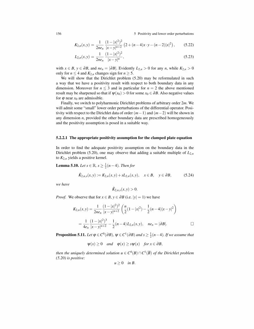
156 5 Positivity and lower order perturbations
K2,n(x,y) =1
2nen
(1−|x|2)2
|x− y|n+2
(2+(n−4)x · y− (n−2)|x|2
), (5.22)
L2,n(x,y) =1
2nen
(1−|x|2)2
|x− y|n, (5.23)
with x ∈ B, y ∈ ∂B, and nen = |∂B|. Evidently L2,n > 0 for any n, while K2,n > 0only for n≤ 4 and K2,n changes sign for n≥ 5.
We will show that the Dirichlet problem (5.20) may be reformulated in sucha way that we have a positivity result with respect to both boundary data in anydimension. Moreover for n ≤ 3 and in particular for n = 2 the above mentionedresult may be sharpened so that if ψ(x0) > 0 for some x0 ∈ ∂B. Also negative valuesfor ϕ near x0 are admissible.
Finally, we switch to polyharmonic Dirichlet problems of arbitrary order 2m. Wewill admit some “small” lower order perturbations of the differential operator. Posi-tivity with respect to the Dirichlet data of order (m−1) and (m−2) will be shown inany dimension n, provided the other boundary data are prescribed homogeneouslyand the positivity assumption is posed in a suitable way.
5.2.2.1 The appropriate positivity assumption for the clamped plate equation
In order to find the adequate positivity assumption on the boundary data in theDirichlet problem (5.20), one may observe that adding a suitable multiple of L2,nto K2,n yields a positive kernel.
Lemma 5.10. Let s ∈ R, s≥ 12 (n−4). Then for
K2,n,s(x,y) := K2,n(x,y)+ sL2,n(x,y), x ∈ B, y ∈ ∂B, (5.24)
we haveK2,n,s(x,y) > 0.
Proof. We observe that for x ∈ B, y ∈ ∂B (i.e. |y|= 1) we have
K2,n(x,y) =1
2nen
(1−|x|2)2
|x− y|n+2
(n2(1−|x|2)− 1
2(n−4)|x− y|2
)
=1
4en
(1−|x|2)3
|x− y|n+2 −12(n−4)L2,n(x,y), nen = |∂B|.
Proposition 5.11. Let ϕ ∈C0(∂B), ψ ∈C1(∂B) and s≥ 12 (n−4). If we assume that
ψ(x)≥ 0 and ϕ(x)≥ sψ(x) for x ∈ ∂B,
then the uniquely determined solution u ∈ C4(B)∩C1(B) of the Dirichlet problem(5.20) is positive:
u≥ 0 in B.
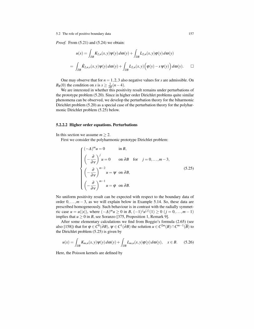
5.2 The role of positive boundary data 157
Proof. From (5.21) and (5.24) we obtain:
u(x) =∫
∂BK2,n(x,y)ψ(y)dω(y)+
∫∂B
L2,n(x,y)ϕ(y)dω(y)
=∫
∂BK2,n,s(x,y)ψ(y)dω(y)+
∫∂B
L2,n(x,y)(
ϕ(y)− sψ(y))
dω(y).
One may observe that for n = 1,2,3 also negative values for s are admissible. OnBR(0) the condition on s is s≥ 1
2R (n−4).We are interested in whether this positivity result remains under perturbations of
the prototype problem (5.20). Since in higher order Dirichlet problems quite similarphenomena can be observed, we develop the perturbation theory for the biharmonicDirichlet problem (5.20) as a special case of the perturbation theory for the polyhar-monic Dirichlet problem (5.25) below.
5.2.2.2 Higher order equations. Perturbations
In this section we assume m≥ 2.First we consider the polyharmonic prototype Dirichlet problem:
(−∆)mu = 0 in B,(− ∂
∂ν
) j
u = 0 on ∂B for j = 0, . . . ,m−3,(− ∂
∂ν
)m−2
u = ψ on ∂B,(− ∂
∂ν
)m−1
u = ϕ on ∂B.
(5.25)
No uniform positivity result can be expected with respect to the boundary data oforder 0, . . . ,m− 3, as we will explain below in Example 5.14. So, these data areprescribed homogeneously. Such behaviour is in contrast with the radially symmet-ric case u = u(|x|), where (−∆)mu ≥ 0 in B, (−1) ju( j)(1) ≥ 0 ( j = 0, . . . ,m− 1)implies that u≥ 0 in B, see Soranzo [375, Proposition 1, Remark 9].
After some elementary calculations we find from Boggio’s formula (2.65) (seealso [158]) that for ϕ ∈C0(∂B), ψ ∈C1(∂B) the solution u ∈C2m(B)∩Cm−1(B) tothe Dirichlet problem (5.25) is given by
u(x) =∫
∂BKm,n(x,y)ψ(y)dω(y)+
∫∂B
Lm,n(x,y)ϕ(y)dω(y), x ∈ B. (5.26)
Here, the Poisson kernels are defined by
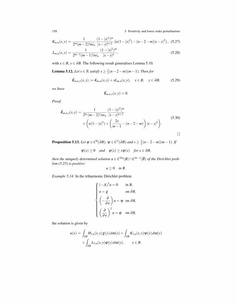
158 5 Positivity and lower order perturbations
Km,n(x,y) =1
2m(m−2)!nen
(1−|x|2)m
|x− y|n+2
(n(1−|x|2)− (n−2−m)|x− y|2
), (5.27)
Lm,n(x,y) =1
2m−1(m−1)!nen
(1−|x|2)m
|x− y|n, (5.28)
with x ∈ B, y ∈ ∂B. The following result generalises Lemma 5.10.
Lemma 5.12. Let s ∈ R satisfy s≥ 12 (n−2−m)(m−1). Then for
Km,n,s(x,y) := Km,n(x,y)+ sLm,n(x,y), x ∈ B, y ∈ ∂B, (5.29)
we haveKm,n,s(x,y) > 0.
Proof.
Km,n,s(x,y) =1
2m (m−2)!nen
(1−|x|2)m
|x− y|n+2
×(
n(1−|x|2)+(
2sm−1
− (n−2−m))|x− y|2
).
(5.30)
Proposition 5.13. Let ϕ ∈C0(∂B), ψ ∈C1(∂B) and s≥ 12 (n−2−m)(m−1). If
ψ(x)≥ 0 and ϕ(x)≥ sψ(x) for x ∈ ∂B,
then the uniquely determined solution u ∈C2m(B)∩Cm−1(B) of the Dirichlet prob-lem (5.25) is positive:
u≥ 0 in B.
Example 5.14. In the triharmonic Dirichlet problem
(−∆)3u = 0 in B,
u = χ on ∂B,(− ∂
∂ν
)u = ψ on ∂B,(
∂
∂ν
)2
u = ϕ on ∂B,
the solution is given by
u(x) =∫
∂BH3,n(x,y)χ(y)dω(y)+
∫∂B
K3,n(x,y)ψ(y)dω(y)
+∫
∂BL3,n(x,y)ϕ(y)dω(y), x ∈ B.

5.2 The role of positive boundary data 159
The kernels K3,n and L3,n are defined above and
H3,n(x,y) =1
16nen
(1−|x|2)3
|x− y|n+4
(n(n+2)(1−|x|2)2 +(n−4)(n−8)|x− y|4
−2n(n−7)(1−|x|2)|x− y|2−4n|x− y|2)
with x ∈ B, y ∈ ∂B. For any n, x → y, x “very close” to the boundary, H3,n takes onalso negative values. By adding multiples of L3,n and K3,n, only the terms |x− y|4and (1−|x|2)|x− y|2 in the curved brackets could be effected. In any case the mostdangerous term −4n|x− y|2 remains.
Theorem 5.15. Let s > 12 (n−2−m)(m−1). Then there exists ε0 = ε0(m,n,s) > 0
such that the following holds.If ‖aβ‖C|β |(B) ≤ ε0 for |β | ≤ 2m−2, then for every ϕ ∈C0(∂B) and ψ ∈C1(∂B)
withψ ≥ 0
ϕ ≥ sψ
on ∂B, ψ 6≡ 0 or ϕ 6≡ 0,
the Dirichlet problem
(−∆)mu+ ∑|β |≤2m−2
aβ (x)Dβ u = 0 in B,(− ∂
∂ν
) j
u = 0 on ∂B for j = 0, . . . ,m−3,(− ∂
∂ν
)m−2
u = ψ on ∂B,(− ∂
∂ν
)m−1
u = ϕ on ∂B,
(5.31)
has a solution u ∈W 2m,ploc (B)∩Cm−1(B) (p > 1 arbitrary) which is strictly positive:
u > 0 in B.
In order to prove this result we first need to describe the essential properties ofthe integral kernels Km,n,s and Lm,n.
Lemma 5.16. 1. Let s ≥ 12 (n− 2−m)(m− 1). On B× ∂B (i.e. for x ∈ B, y ∈ ∂B)
we have
Km,n,s(x,y)
|x− y|−n−1d(x)m,
|x− y|−n−2d(x)m+1,(5.32)
Lm,n(x,y)' |x− y|−nd(x)m. (5.33)
2. If we assume additionally that s > 12 (n−2−m)(m−1), then we have on B×∂B:
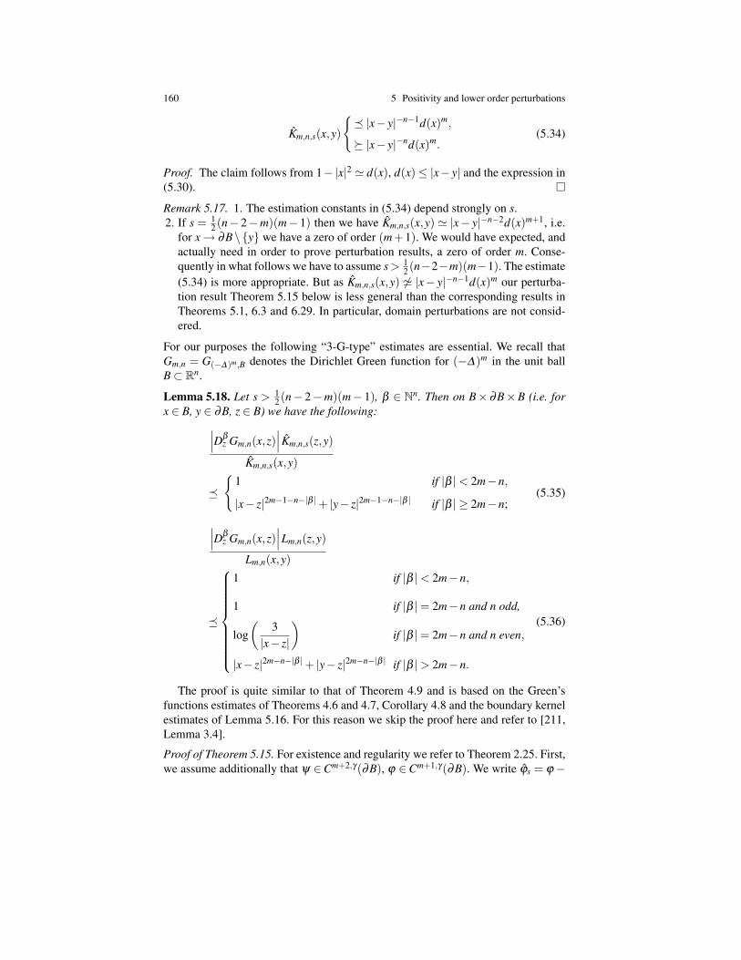
160 5 Positivity and lower order perturbations
Km,n,s(x,y)
|x− y|−n−1d(x)m,
|x− y|−nd(x)m.(5.34)
Proof. The claim follows from 1−|x|2 ' d(x), d(x)≤ |x− y| and the expression in(5.30).
Remark 5.17. 1. The estimation constants in (5.34) depend strongly on s.2. If s = 1
2 (n− 2−m)(m− 1) then we have Km,n,s(x,y) ' |x− y|−n−2d(x)m+1, i.e.for x→ ∂B\y we have a zero of order (m+1). We would have expected, andactually need in order to prove perturbation results, a zero of order m. Conse-quently in what follows we have to assume s > 1
2 (n−2−m)(m−1). The estimate(5.34) is more appropriate. But as Km,n,s(x,y) 6' |x− y|−n−1d(x)m our perturba-tion result Theorem 5.15 below is less general than the corresponding results inTheorems 5.1, 6.3 and 6.29. In particular, domain perturbations are not consid-ered.
For our purposes the following “3-G-type” estimates are essential. We recall thatGm,n = G(−∆)m,B denotes the Dirichlet Green function for (−∆)m in the unit ballB⊂ Rn.
Lemma 5.18. Let s > 12 (n− 2−m)(m− 1), β ∈ Nn. Then on B× ∂B×B (i.e. for
x ∈ B, y ∈ ∂B, z ∈ B) we have the following:∣∣∣Dβz Gm,n(x,z)
∣∣∣ Km,n,s(z,y)
Km,n,s(x,y)
1 if |β |< 2m−n,
|x− z|2m−1−n−|β |+ |y− z|2m−1−n−|β | if |β | ≥ 2m−n;(5.35)
∣∣∣Dβz Gm,n(x,z)
∣∣∣Lm,n(z,y)
Lm,n(x,y)
1 if |β |< 2m−n,
1 if |β |= 2m−n and n odd,
log(
3|x− z|
)if |β |= 2m−n and n even,
|x− z|2m−n−|β |+ |y− z|2m−n−|β | if |β |> 2m−n.
(5.36)
The proof is quite similar to that of Theorem 4.9 and is based on the Green’sfunctions estimates of Theorems 4.6 and 4.7, Corollary 4.8 and the boundary kernelestimates of Lemma 5.16. For this reason we skip the proof here and refer to [211,Lemma 3.4].
Proof of Theorem 5.15. For existence and regularity we refer to Theorem 2.25. First,we assume additionally that ψ ∈Cm+2,γ(∂B), ϕ ∈Cm+1,γ(∂B). We write ϕs = ϕ−
5.2 The role of positive boundary data 161
sψ and let p > 1 be arbitrary. The operator
Lm,nϕs(x) :=∫
∂BLm,n(x,y)ϕs(y)dω(y)
satisfies Lm,n : Cm+1,γ(∂B)→C2m,γ(B)⊂W 2m,p(B), the operator
ˆKm,n,sψ(x) :=∫
∂BKm,n,s(x,y)ψ(y)dω(y)
satisfies ˆKm,n,s : Cm+2,γ(∂B)→C2m,γ(B)⊂W 2m,p(B), while the Green operator
Gm,n f (x) :=∫
BGm,n(x,y) f (y)dy
satisfies Gm,n : Lp(B)→W 2m,p ∩W m,p0 (B), see Theorem 2.19 and Corollary 2.21.
We write A := ∑|β |≤2m−2 aβ ( .)Dβ . The solution of (5.31) is given by
u =−Gm,nA u+ ˆKm,n,sψ +Lm,nϕs or (I +Gm,nA )u = ˆKm,n,sψ +Lm,nϕs.
Here, I +Gm,nA is a bounded linear operator in W 2m,p(B) which for sufficientlysmall ε0 is invertible. Hence
u = (I +Gm,nA )−1 ˆKm,n,sψ +(I +Gm,nA )−1 Lm,nϕs
= ˆKm,n,sψ +∞
∑i=1
(−Gm,nA )i ˆKm,n,sψ +Lm,nϕs +∞
∑i=1
(−Gm,nA )i Lm,nϕs.
We only show how to deal with the first Neumann series containing ˆKm,n,s, thesecond series containing Lm,n can be treated in the same way with some obvioussimplifications. For i ≥ 1 we integrate by parts. As A is of order ≤ 2m− 2 and
ˆKm,n,sψ vanishes on ∂B of order m− 2 no additional boundary integrals arise. Bymeans of the Fubini-Tonelli theorem we obtain for x ∈ B
(−Gm,nA )i ˆKm,n,sψ(x) = (−1)i∫
z1∈BGm,n(x,z1) Az1
∫z2∈B
Gm,n(z1,z2)
× . . . Azi−1
∫zi∈B
Gm,n(zi−1,zi) Azi
∫y∈∂B
Km,n,s(zi,y)ψ(y)dω(y)dzi . . .dz1
= (−1)i∫
z1∈B
(A ∗
z1Gm,n(x,z1)
)∫z2∈B
(A ∗
z2Gm,n(z1,z2)
)× . . .
∫zi∈B
(A ∗
ziGm,n(zi−1,zi)
)∫y∈∂B
Km,n,s(zi,y)ψ(y)dω(y)dzi . . .dz1
= (−1)i∫
B· · ·∫
B
∫∂B
(A ∗
z1Gm,n(x,z1)
)(A ∗
z2Gm,n(z1,z2)
)× . . .
(A ∗
ziGm,n(zi−1,zi)
)Km,n,s(zi,y)ψ(y)dω(y)d(z1, . . . ,zi).
162 5 Positivity and lower order perturbations
Here A ∗. = ∑|β |≤2m−2(−1)|β |Dβ (aβ . ) is the (formally) adjoint operator of the
perturbation A . The estimates (5.35) and (5.36) in Lemma 5.18 are integrable withrespect to z ∈ B uniformly in x ∈ B, y ∈ ∂B if |β | ≤ 2m−2. They yield∣∣∣(−Gm,nA )i ˆKm,n,sψ(x)
∣∣∣≤∫
∂B
∫B· · ·∫
BKm,n,s(x,y)
∣∣A ∗z1
Gm,n(x,z1)∣∣ Km,n,s(z1,y)
Km,n,s(x,y)
×∣∣A ∗
z2Gm,n(z1,z2)
∣∣ Km,n,s(z2,y)
Km,n,s(z1,y)
× . . .
∣∣A ∗zi
Gm,n(zi−1,zi)∣∣ Km,n,s(zi,y)
Km,n,s(zi−1,y)ψ(y)d(z1, . . . ,zi)dω(y)
≤ (C0ε0)i∫
∂BKm,n,s(x,y)ψ(y)dω(y) = (C0ε0)
i ( ˆKm,n,sψ)(x).
Analogously we have:∣∣∣(−Gm,nA )i Lm,nϕs(x)∣∣∣≤ (C0ε0
)i (Lm,nϕs)(x).
The constants C0 = C0(m,n,s), C0 = C0(m,n) do not depend on i.If ε0 = ε0(m,n,s) > 0 is chosen sufficiently small, we come up with
u≥ 1C
ˆKm,n,sψ +1C
Lm,nϕs. (5.37)
The general case ϕ ∈ C0(∂B), ψ ∈ C1(∂B) follows from (5.37) with the help ofan approximation, the maximum modulus estimates of Theorem 2.25 and local Lp-estimates, see Theorem 2.20.
5.3 Local maximum principles for higher order differentialinequalities
The comparison results of Section 5.1 together with the observations of Section 5.2on the Poisson boundary kernels will yield local maximum principles for differen-tial inequalities, which are valid for a large class of operators. Here lower orderperturbations are no longer subject to smallness restrictions.
We consider C2m,γ -smooth domains Ω ⊂ Rn and differential operators L like
Lu :=
(−
n
∑i, j=1
ai j∂ 2
∂xi∂x j
)m
u+ ∑|β |≤2m−1
aβ ( .)Dβ u, (5.38)
with constant highest order coefficients ai j = a ji obeying the ellipticity condition
5.3 Local maximum principles for higher order differential inequalities 163
λ |ξ |2 ≤n
∑i, j=1
ai jξiξ j ≤Λ |ξ |2 for all ξ ∈ Rn.
The ellipticity constants are subject to the condition 0 < λ ≤ Λ . The lower ordercoefficients are merely assumed to be smooth,
aβ ∈C|β |,γ(Ω).
Under these assumptions, we have:
Theorem 5.19. Assume that q ≥ 1, q > n2m and that K ⊂ Ω is a compact subset.
Then there exists a constant
C = C(
n,m,λ ,Λ ,q, max|β |≤2m−1
‖aβ‖C|β |(Ω),dist(K,∂Ω))
such that, for every f ∈C0(Ω) and every subsolution u ∈C2m(Ω) of the differentialinequality
Lu≤ f ,
the following local maximum estimate holds true:
supK
u≤C(‖ f +‖Lq +‖u‖W m−1,1
). (5.39)
Proof. With the help of a linear transformation we may achieve ai j = δi j. So, inwhat follows we consider the principal part (−∆)m.
We want to apply Theorem 5.4 and Lemma 5.9. Let ε0 = ε0(m,n) > 0 besuch that both results hold true in the unit ball B for all differential operatorsL = (−∆)m + ∑|β |≤2m−1 aβ Dβ with max|β |≤2m−1 ‖aβ‖C|β |(B) ≤ ε0. For the differ-
ential operator L = (−∆)m + ∑|β |≤2m−1 aβ Dβ defined in Ω we want to achieve therequired smallness by means of scaling.
Let x0 ∈ K be arbitrary, after translation we may assume x0 = 0. We put
M := max|β |≤2m−1
‖aβ‖C|β |(Ω),
ρ0 := min
1,12
dist(K,∂Ω),ε0
M
. (5.40)
For ρ ∈ (0,ρ0] we introduce the following scaled functions B→ R:
uρ(x) := u(ρx), fρ(x) := ρ2m f (ρx), aβ ,ρ(x) := ρ
2m−|β |aβ (ρx).
For these functions we have on B the following differential inequality
Lρ uρ(x) := (−∆)muρ(x)+ ∑|β |≤2m−1
aβ ,ρ(x)Dβ uρ(x)≤ fρ(x). (5.41)
164 5 Positivity and lower order perturbations
Here, thanks to our choice (5.40) of ρ0, on B the coefficients aβ ,ρ , |β | ≤ 2m−1, aresubject of the following smallness condition
‖aβ ,ρ‖C|β |(B) = ∑|µ|≤|β |
maxx∈B
∣∣Dµ aβ ,ρ(x)∣∣= ∑
|µ|≤|β |maxx∈B
(ρ
2m−|β |+|µ| ∣∣(Dµ aβ
)(ρx)
∣∣)≤ ρ0‖aβ‖C|β |(Ω) ≤ ρ0M ≤ ε0.
Let GLρ ,B be the Green function for Lρ in B. Theorem 5.4 and Lemma 5.9 show thatthere exist constants C = C (m,n,ε0(m,n)) = C(m,n), independent of ρ ∈ (0,ρ0],such that we have:
GLρ ,B(x,y) > 0 in B×B,
GLρ ,B(x,y)≤C|x− y|2m−n in B×B if n > 2m,
GLρ ,B(x,y)≤C log(
3|x− y|
)in B×B if n = 2m,
GLρ ,B(x,y)≤C in B×B if n < 2m,∣∣∣Dβy GLρ ,B(0,y)
∣∣∣≤C for |β | ≤ 2m−1, y ∈ ∂B.
(5.42)
To estimate u(0) = uρ(0) we use the representation formula for uρ . Beside theDirichlet data Dβ uρ , |β | ≤ m− 1 and terms of the kind Dβ
y GLρ ,B(0,y), m ≤ |β | ≤2m− 1, the boundary integrals contain factors aβ ,ρ and their derivatives up toorder ≤ max0, |β | −m− 1. Making use of (5.42), we obtain independently ofρ ∈ (0,ρ0]:
u(0) = uρ(0)≤∫
BGLρ ,B(0,y) f +
ρ (y)dy
+ C(m,n,M) ∑|β |≤m−1
∫∂B
∣∣∣Dβ uρ(y)∣∣∣ dω(y)
≤ C(m,n,q)‖ f +ρ ‖Lq(B) +C(m,n,M) ∑
|β |≤m−1ρ|β |∫
∂B
∣∣∣(Dβ u)
(ρy)∣∣∣ dω(y)
≤ C(m,n,q)ρ2m−(n/q)‖ f +‖Lq(Bρ )
+ C(m,n,M) ∑|β |≤m−1
ρ|β |−n+1
∫|y|=ρ
∣∣∣Dβ u(y)∣∣∣ dω(y).
Integration with respect to ρ ∈ [ 12 ρ0,ρ0] yields
u(0)≤C(‖ f +‖Lq(Ω) +‖u‖W m−1,1(Ω)
)with a constant C = C(m,n,q,M,ρ0). Here C = O(ρ−n
0 ) for ρ0 0.
Remark 5.20. This local maximum principle may also be applied to nonlinearproblems which are not subject to the standard (controllable) growth conditions
5.4 Steklov boundary conditions 165
as in [404, 405], see [209]. For instance, one finds “almost” classical solutionsu ∈C2m,γ(Ω)∩Hm
0 (Ω) to the Dirichlet problem for Lu = eu where L is as in (5.38).
5.4 Steklov boundary conditions
Let Ω be a bounded domain of Rn (n≥ 2) with ∂Ω ∈C2 and consider the boundaryvalue problem
∆ 2u = f in Ω ,
u = ∆u−a ∂u∂ν
= 0 on ∂Ω ,(5.43)
where a ∈C0(∂Ω), f ∈ L2(Ω) and ν is the outside normal (we will also use uν =∂u∂ν
). In this section we study the positivity preserving property for (5.43), namelyunder which conditions on Ω and on the boundary coefficient a the assumptionf ≥ 0 implies that the solution u exists and is positive. Let us first make precisewhat is meant by a solution of (5.43).
Definition 5.21. For f ∈ L2(Ω) we say that u is a weak solution of (5.43) if u ∈H2∩H1
0 (Ω) and∫Ω
∆u∆v dx−∫
∂Ω
a uν vν dω =∫
Ω
f v dx for all v ∈ H2∩H10 (Ω). (5.44)
Note that weak solutions are well-defined for a ∈C0(∂Ω). For u ∈ H4(Ω) onemay integrate by parts to find indeed that a weak solution of (5.44) satisfies theboundary value problem in (5.43). This means that the second boundary conditionin (5.43) is hidden in the choice of the space H2 ∩H1
0 (Ω) of admissible testingfunctions. For regularity results related to problem (5.43) we refer to Corollary 2.23.
In the next section we state the positivity preserving properties for (5.43) andwe give the first part of their proof. The second part of their proof is more delicateand requires a Schauder setting and a different notion of solution. This is the reasonwhy it is postponed to Section 5.4.3. In turn, the Schauder setting takes advantageof the positivity properties of the operators involved in the solution of (5.43). Theseproperties are proven in Section 5.4.2 with a strong use of the kernel estimates ofSection 4.3.
5.4.1 Positivity preserving
The first statement describes existence, uniqueness and positivity of a weak solutionto (5.43). A crucial role is played by a “weighted first eigenvalue”. Fix a nontrivialpositive weight function b ∈C0(∂Ω) and set
Jb(u) =∫
Ω|∆u|2 dx∫
∂Ωb u2
ν dωfor
∫∂Ω
b u2ν dω 6= 0 (5.45)
166 5 Positivity and lower order perturbations
and Jb(u) = ∞ otherwise. For every u ∈ H2 ∩H10 (Ω) the functional in (5.45) is
strictly positive, possibly ∞. Since the linear map H2(Ω) → L2(∂Ω) defined byu 7→ uν |∂Ω is compact, there exists a minimiser for the problem
δ1,b = δ1,b(Ω) := infu∈H2∩H1
0 (Ω)Jb(u). (5.46)
Hence δ1,b > 0 and it may be viewed as a kind of first Steklov eigenvalue with re-spect to the weight function b and any minimiser as a corresponding eigenfunction.This definition should be compared with (3.40) in Section 3.3.1.
The next statement summarises the positivity preserving results for (5.43), seethe Notations-Section for the interpretation of the symbols.
Theorem 5.22. Let Ω ⊂ Rn (n ≥ 2) be a bounded domain with ∂Ω ∈ C2 and let0 b ∈C0(∂Ω). Let the eigenvalue δ1,b be as defined in (5.46). Then there existsa number δc,b := δc,b(Ω) ∈ [−∞,0) such that the following holds for any functiona ∈C0(∂Ω).
1. If a ≥ δ1,bb and if 0 f ∈ L2(Ω), then (5.43) has no nontrivial positive weaksolution.
2. If a = δ1,bb, then there exists a positive eigenfunction, that is, problem (5.43) withf = 0 admits a weak solution u1,b that satisfies u1,b > 0 and −∆u1,b > 0 in Ω ,∂
∂νu1,b < 0 on ∂Ω . This eigenfunction u1,b is unique, up to a constant multiplier.
3. If a δ1,bb, then for any f ∈ L2(Ω) problem (5.43) admits a unique weak solu-tion u.
a. If δc,bb≤ a δ1,bb and if 0 f ∈ L2(Ω), then u 0.b. If δc,bb < a δ1,bb and if 0 f ∈ L2(Ω), then for some c f > 0 it holds that
u≥ c f d with d as in (4.1). Furthermore, if a(x0) < 0 for some x0 ∈ ∂Ω , then−∆u 0 in Ω , whereas if a≥ 0, then 0 f implies −∆u≥ 0 in Ω .
c. If a < δc,bb, then there are 0 f ∈ L2(Ω) such that the corresponding solutionu of (5.43)is not positive: 0 u.
Proof. We first prove Item 2, then Item 1 and we end with Item 3.Proof of Item 2. Let u1 := u1,b ∈ H2 ∩H1
0 (Ω) be a minimiser for (5.46) and letu1 be the unique solution in H2∩H1
0 (Ω) of −∆ u1 = |∆u1|. Then by the maximum
principle we infer that |u1| ≤ u1 in Ω and∣∣∣ ∂
∂νu1
∣∣∣≤ ∣∣∣ ∂
∂νu1
∣∣∣ on ∂Ω . If ∆u1 changessign, then these inequalities are strict and imply Jb(u1) > Jb(u1). Hence, ∆u1 is offixed sign, say −∆u1 ≥ 0, so that the maximum principle implies ∂
∂νu1 < 0 on ∂Ω
and u1 ≥ cd in Ω , where d is as in (4.1). Similarly, if u1 and u2 are two minimiserswhich are not multiples of each other, then there is a linear combination which isa sign changing minimiser and one proceeds as above to find a contradiction. Thisproves Item 2.
Proof of Item 1. Let us suppose by contradiction that a ≥ δ1,b, that f 0 andthat u is a nontrivial positive solution to (5.43). Hence uν ≤ 0 on ∂Ω . Let u1,b be aminimiser for (5.46) as obtained above. By taking v = u1,b in (5.44) one finds
5.4 Steklov boundary conditions 167
0 <∫
Ω
f u1,b dx =∫
Ω
∆u∆u1,b dx−∫
∂Ω
a uν
(u1,b)
νdω
≤∫
Ω
∆u∆u1,b dx−∫
∂Ω
δ1,b b uν
(u1,b)
νdω = 0,
a contradiction. The last equality follows by the fact that u1,b minimises (5.46). Thisproves Item 1.
Proof of Item 3. On the space H2∩H10 (Ω) we define the energy functional
I(u) := 12
∫Ω
|∆u|2 dx− 12
∫∂Ω
au2ν dω−
∫Ω
f u dx u ∈ H2∩H10 (Ω).
Critical points of I are weak solutions of (5.43) in the sense of Definition 5.21. Wewill show that for a δ1,bb the functional I has a unique critical point.
If a < δ1,bb, one sets
ε :=min
δ1,bb(x)−a(x); x ∈ ∂Ω
max
δ1,bb(x); x ∈ ∂Ω
> 0, (5.47)
and finds that a ≤ (1− ε)δ1,bb. By the definition of δ1,b we have for all u ∈ H2 ∩H1
0 (Ω) ∫Ω
|∆u|2 dx−∫
∂Ω
a u2ν dω
≥ ε
∫Ω
|∆u|2 dx+(1− ε)(∫
Ω
|∆u|2 dx−∫
∂Ω
δ1,bb u2ν dω
)(5.48)
≥ ε
∫Ω
|∆u|2 dx,
so that the functional I is coercive. Since it is also strictly convex the functional Iadmits a unique critical point which is its global minimum over H2∩H1
0 (Ω).In order to deal with the case that a+ δ1,bb, but a+(x) = δ1,bb(x) for some
x ∈ ∂Ω , we set
b :=12
(b+δ
−11,b a+
).
Let u1 be a minimiser of Jb and u2 of Jb. For the definition see (5.45). Then, since
0 b b and(
∂
∂νu1
)2> 0 on ∂Ω , we find δ1,b = Jb(u1) > Jb(u1)≥ Jb(u2) = δ1,b.
Instead of (5.47) we setε := 1−δ1,b/δ1,b > 0,
find for x ∈ ∂Ω that a ≤ a+ = δ1,b(2b− b) ≤ δ1,bb = (1− ε)δ1,bb and proceed byreplacing all b in (5.48) with b.
If a+ = δ1,bb and a− 0, then one may not proceed directly as before. However,instead of the functional in (5.45), one may use

168 5 Positivity and lower order perturbations
Ja−b (u) =
(∫Ω
|∆u|2 dx+∫
∂Ω
a− u2ν dω
) (∫∂Ω
b u2ν dω
)−1
.
Then, defining δ a−1,b for Ja−
b as in (5.46), this minimum is assumed, say by ua−1,b. Since
δa−1,b = Ja−
b (ua−1,b)≥ Jb(ua−
1,b)≥ Jb(u1,b) = δ1,b,
with the last inequality strict if ua−1,b 6= c u1,b and with the first inequality strict if
ua−1,b = c u1,b since (u1,b)2
ν > 0, we find δ a−1,b > δ1,b. So,∫
Ω
|∆u|2 dx+∫
∂Ω
a− u2ν dω ≥ δ
a−1,b
∫∂Ω
b u2ν dω for all u ∈ H2∩H1
0 (Ω)
and by settingε := 1−δ1,b/δ
a−1,b > 0
we find the result that replaces (5.48). Indeed∫Ω
|∆u|2 dx−∫
∂Ω
a u2ν dω =
∫Ω
|∆u|2 dx+∫
∂Ω
a− u2ν dω−
∫∂Ω
δ1,bb u2ν dω
≥ ε
∫Ω
|∆u|2 dx+(1− ε)(∫
Ω
|∆u|2 dx+∫
∂Ω
a− u2ν dω−
∫∂Ω
δa−1,b b u2
ν dω
)≥ ε
∫Ω
|∆u|2 dx.
Hence, I is coercive and strictly convex and we conclude as for (5.48). The existenceand uniqueness is so proved.
Assume now that there exists x0 ∈ ∂Ω such that a(x0) < 0. If the weak solutionu were superharmonic, then by Hopf’s boundary lemma we would have uν(x0) < 0.Using the second boundary condition in (5.43), we would then obtain ∆u(x0) > 0,a contradiction.
If a≥ 0 and f 0, let u be the unique solution in H2∩H10 (Ω) of −∆ u = |∆u| in
Ω . Since u > u or u = u in Ω , and |uν | ≥ |uν | on ∂Ω , one finds for f 0 that
I(u)− I(u) =−12
∫∂Ω
a(u2
ν −u2ν
)dω−
∫Ω
f (u−u) dx≤ 0.
Equality occurs only when u = u. Since I is strictly convex there is at most onecritical point which is a minimum. So u = u > 0 and −∆u =−∆ u = |∆u| ≥ 0. Thiscompletes the proof of existence and uniqueness whenever a δ1,bb. The proof ofthe remaining statements (a), (b), (c) in Item 3 is more lengthy and delicate and wegive it in Section 5.4.3, see Theorem 5.37.
Note that in Theorem 5.22 it may happen that b(x) = 0 on some part Γ1 ⊂ ∂Ω
and b(x) > 0 on the remaining part Γ0 = ∂Ω \Γ1. If moreover δc,b = −∞, then thelimit problem for which the positivity preserving property holds (that is, a = δc,bb)becomes a mixed Dirichlet-Navier problem with boundary conditions

5.4 Steklov boundary conditions 169
u = 0 on ∂Ω , uν = 0 on Γ0, ∆u = 0 on Γ1.
As a first consequence of Theorem 5.22 we have the positivity preserving prop-erty for the hinged plate model in planar convex domains. As we have seen in Sec-tion 1.1.2, the physical bounds for the Poisson ratio are given by
−1 < σ < 1 . (5.49)
Under this constraint, the following result holds.
Corollary 5.23. Let Ω ⊂ R2 be a bounded convex domain with C2-boundary andassume (5.49). For any f ∈ L2(Ω) there exists a unique minimiser u ∈ H2∩H1
0 (Ω)of the elastic energy functional (1.11) that is, of
J(u) =∫
Ω
(|∆u|2
2− f u
)dx− 1−σ
2
∫∂Ω
κ u2ν dω,
where κ denotes the curvature of ∂Ω . The minimiser u is the unique weak solutionto
∆ 2u = f in Ω ,u = ∆u− (1−σ)κuν = 0 on ∂Ω .
Moreover, f 0 implies that there exists c f > 0 such that u(x) ≥ c f d(x) and u issuperharmonic in Ω .
Proof. We first show that the energy functional J coincides with the form given in(1.5). This can be done on a dense subset of smooth functions. Since u|∂Ω = 0, onehas ux = uν ν1 and uy = uν ν2 and may conclude that
2∫
Ω
(u2
xy−uxxuyy)
dxdy
=∫
∂Ω
(uxyuyν1 +uxyuxν2−uxxuyν2−uyyuxν1) dω
=∫
∂Ω
uν
(2uxyν1ν2−uxxν
22 −uyyν
21)
dω =−∫
∂Ω
κu2ν dω,
where in the last step we used (1.8). Hence, existence and uniqueness of a minimiseru follow from Proposition 2.35.
Since ∂Ω ∈C2 and Ω is convex we have 0 κ ∈C0(∂Ω). In Proposition 2.35,it is also shown that J is strictly convex so that (1−σ)κ δ1,κ κ . Hence, if f 0it follows first from statement 3.(a) in Theorem 5.22 that u 0 in Ω and so thatuν |∂Ω ≤ 0. In view of the boundary value problem solved by u we obtain −∆u 0in Ω . This superharmonicity finally yields the other properties stated for u.
More generally, if we take b = 1 in Theorem 5.22, we obtain the following
Corollary 5.24. Let Ω ⊂ Rn (n≥ 2) be a bounded domain with ∂Ω ∈C2 and let
δ1 := δ1(Ω) := inf∫
Ω|∆u|2 dx∫
∂Ωu2
ν dω; u ∈ H2∩H1
0 (Ω)\H20 (Ω)
∈ (0,∞) (5.50)
170 5 Positivity and lower order perturbations
be the first Steklov eigenvalue. Then there exists a number δc := δc(Ω) ∈ [−∞,0)such that the following holds for any function a ∈C0(∂Ω).
1. If a ≥ δ1 and if 0 f ∈ L2(Ω), then (5.43) has no nontrivial positive weaksolution.
2. If a = δ1, then there exists a positive eigenfunction, that is, problem (5.43) admitsa nontrivial weak solution u1 with u1 > 0 in Ω for f = 0. Moreover, the functionu1 is, up to multiples, the unique solution of (5.43) with f = 0 and a = δ1.
3. If a δ1, then for any f ∈ L2(Ω) problem (5.43) admits a unique weak solutionu.
a. If δc ≤ a δ1, then 0 f ∈ L2(Ω) implies u 0 in Ω .b. If δc < a δ1, then 0 f ∈ L2(Ω) implies u≥ c f d > 0 in Ω for some c f > 0.c. If a < δc, then there are 0 f ∈ L2(Ω) with 0 u.
The result described in Corollary 5.24 quite closely resembles the structure forthe resolvent of the biharmonic operator under Navier boundary conditions – seeMcKenna-Walter [297] and Kawohl-Sweers [246] – or for the biharmonic operatorunder Dirichlet boundary conditions in case the domain is a ball – see Corollary 5.5where (−a) plays the same role as a here. For all these problems the scheme is asfollows.
∃ f > 0 with u 0 ∀ f > 0 : ∃u and u≥ 0 ∀ f > 0 if ∃u then u 0
0δc δ1 a−→
Under Dirichlet boundary conditions such that the corresponding Green functionis positive, Corollary 5.5 tells us that the set of constant coefficients a∈R for which∆ 2u ≥ au implies u ≥ 0 is an interval (ac,Λ2,1) with ac ∈ (−∞,0]. By combiningTheorem 5.22 with Lemma 5.35 below, we immediately see that a similar resultholds for (5.43).
Theorem 5.25. Let Ω ⊂ Rn (n ≥ 2) be a bounded domain with ∂Ω ∈ C2 and letai ∈C0(∂Ω) with i = 1,2. Suppose that a1 ≤ 0 ≤ a2 are such that both for a = a1and a = a2 we have the following: for all f ∈ L2(Ω) there exists a weak solutionu = ui (i = 1,2) for (5.43), and moreover
f 0 implies u 0. (5.51)
Then for any a ∈C0(∂Ω) satisfying a1 ≤ a≤ a2 and for each f ∈ L2(Ω), a uniqueweak solution of (5.43) exists and (5.51) holds true.
However, a crucial difference with the Dirichlet boundary value problem for∆ 2u ≥ au is that ac ∈ (−∞,0] while for problem (5.43) it might happen thatδc(Ω) = −∞ although for general domains one cannot expect to have the posi-tivity preserving property for any negative a. This is stated in the next results which
5.4 Steklov boundary conditions 171
show that the limit situation where δc(Ω) = −∞ is closely related to the positivitypreserving property for the biharmonic Dirichlet problem
∆ 2u = f in Ω ,u = uν = 0 on ∂Ω .
(5.52)
To this end, let us recall once more that the positivity preserving property doesnot hold in general domains Ω ⊂ Rn for (5.52), see Section 1.2. It is clear that(5.43) with |a|= +∞ corresponds to (5.52). However, if a→+∞ then a crosses thespectrum of −∆ under Steklov boundary conditions, see Theorem 3.18, whereasthe next statement justifies the feeling that (5.52) only corresponds to the limit casea =−∞.
Theorem 5.26. Let Ω ⊂Rn (n≥ 2) be a bounded domain with ∂Ω ∈C2. If for everym ∈ N+ and 0 f ∈ L2(Ω) the weak solution of (5.43) with a = −m is nontrivialand positive, then for every 0 f ∈ L2(Ω) the solution u∈H2
0 (Ω) of (5.52) satisfiesu 0.
Proof. Let us first recall the two boundary value problems addressed in the state-ment, namely
∆ 2u = f in Ω ,
u =(
∆ +m ∂
∂ν
)u = 0 on ∂Ω ,
and
∆ 2u = f in Ω ,u = uν = 0 on ∂Ω ,
(5.53)
For all m > 0 let um ∈ H2∩H10 (Ω) be the unique weak solution of the problem on
the left in (5.53). Then according to (5.44) we have∫Ω
∆um∆φ dx+m∫
∂Ω
∂um
∂ν
∂φ
∂νdω =
∫Ω
f φ dx for all φ ∈ H2∩H10 (Ω) . (5.54)
Taking φ = um in (5.54) and using Holder and Poincare inequalities, gives for allm > 0
‖∆um‖2L2 ≤‖∆um‖2
L2 +m∫
∂Ω
∣∣∣∣∂um
∂ν
∣∣∣∣2 dω =∫
Ω
f um dx≤ c‖ f‖L2‖∆um‖L2 . (5.55)
Inequality (5.55) shows that the sequence (um) is bounded in H2(Ω) so that, up toa subsequence, we have
um u in H2(Ω) as m→ ∞ (5.56)
for some u ∈ H2∩H10 (Ω). Once boundedness is established, if we let m → ∞ then
(5.55) also tells us that
∂um
∂ν→ 0 in L2(∂Ω) as m→ ∞ .
172 5 Positivity and lower order perturbations
Therefore, u ∈H20 (Ω). Now take any function φ ∈H2
0 (Ω) in (5.54) and let m→ ∞.By (5.56) we obtain∫
Ω
∆u∆φ dx =∫
Ω
f φ dx for all φ ∈ H20 (Ω) .
Hence, u is the unique solution of the corresponding Dirichlet problem (5.52). Since(5.56) also implies that, up to a subsequence, um(x)→ u(x) for a.e. x ∈Ω , one findsthat u 0.
Theorem 5.26 states that there exists some link between the Steklov and theDirichlet problems. This link is confirmed by the special case when Ω is the unitball. In this case, from Theorem 3.20 we know that the first Steklov eigenvalue asdefined in (5.50) satisfies δ1 = n and the following holds.
Theorem 5.27. Let Ω = B, the unit ball in Rn (n≥ 2). Then, for all 0 f ∈ L2(B)and all a ∈C0(∂B) such that a n, there exists c > 0 such that the weak solution uof (5.43) satisfies u(x)≥ cd(x) in B.
The constant c depends both on f and a, c = c f ,a. For a fixed 0 f ∈ L2(B) weexpect that c = c f ,a → 0 as a→−∞.
Also the proof of Theorem 5.27 requires a Schauder setting and an approximationprocedure. For this reason it is postponed to the end of Section 5.4.3.
5.4.2 Positivity of the operators involved in the Steklov problem
We consider the second order Green operator G and the Poisson operator K , thatis, w = G f +K g formally solves
−∆w = f in Ω ,w = g on ∂Ω .
For C2-domains, the operators G and K can be represented by integral kernels Gand K, see (4.46) in Section 4.3. Let (Pw)(x) :=−ν ·∇w(x) =−wν(x) for x∈ ∂Ω .In this section we use the kernel estimates obtained in Section 4.3 in order to provesome positivity properties of these operators. First, we fix the appropriate setting sothat G , K and P are well-defined operators.
Notation 5.28 Let d denote the distance to ∂Ω as defined in (4.1). Set
Cd(Ω) =
u ∈C0(Ω); there exists w ∈C0(Ω) such that u = dw
with norm
‖u‖Cd(Ω) = sup|u(x)|d(x)
;x ∈Ω
.
Set also C0(Ω) =
u ∈C0(Ω); u = 0 on ∂Ω
so that Cd(Ω) ( C0(Ω).
5.4 Steklov boundary conditions 173
We consider the three above operators in the following setting.
G : C0(Ω)→Cd(Ω), K : C0(∂Ω)→C0(Ω), P : Cd(Ω)→C0(∂Ω).
We also define the embedding
Id : Cd(Ω)→C0(Ω). (5.57)
The space Cd(Ω) is a Banach lattice, that is, a Banach space with the orderingsuch that |u| ≤ |v| implies ‖u‖Cd(Ω) ≤ ‖v‖Cd(Ω), see Definition 3.2 or [13, 309, 359].The positive cone
Cd(Ω)+ =
u ∈Cd(Ω); u(x)≥ 0 in Ω
is solid (namely, it has nonempty interior) and reproducing (that is, every w∈Cd(Ω)can be written as w = u−v for some u,v∈Cd(Ω)+). Similarly, we define C0(∂Ω)+
and C0(Ω)+.Note that the interiors of the cones in these spaces are as follows:
C0(∂Ω)+, =
v ∈C0(∂Ω); v(x)≥ c for some c > 0
,
C0(Ω)+, =
u ∈C0(Ω); u(x)≥ c for some c > 0
,
Cd(Ω)+, =
u ∈Cd(Ω); u(x)≥ cd(x) for some c > 0
.
Definition 5.29. The operator F : C1 → C2 is called
• nonnegative, F ≥ 0, when g ∈ C +1 ⇒Fg ∈ C +
2 ;• strictly positive, F 0, when g ∈ C +
1 \0⇒Fg ∈ C +2 \0;
• strongly positive, F > 0, when g ∈ C +1 \0⇒Fg ∈ C +,
2 .
If F ≥ 0 and F 6= 0, that is, for some g ∈ C +1 we find Fg 0, we call F posi-
tive. Similarly, two operators are ordered through≥ (respectively or >) whenevertheir difference is nonnegative (respectively strictly or strongly positive).
We now prove a positivity result.
Proposition 5.30. Suppose that ∂Ω ∈ C2 and a ∈ C0(∂Ω). Let G , K and P bedefined as above. Then G K aP : Cd(Ω)→Cd(Ω) is a well-defined compact linearoperator. If in addition a 0, then G K aP is positive and even such that
u ∈Cd(Ω)+ implies either G K aPu = 0 or G K aPu ∈Cd(Ω)+,.(5.58)
Proof. Take γ ∈ (0,1), p > n(1−γ)−1 and fix the embeddings I1 : C0(Ω)→ Lp(Ω),I2 : W 2,p(Ω)→C1,γ(Ω) and I3 : C1,γ ∩C0(Ω)→Cd(Ω). Since ∂Ω ∈C2, for everyp ∈ (1,∞) there exists a bounded linear operator Gp : Lp(Ω) → W 2,p ∩W 1,p
0 (Ω)such that −∆Gp f = f for all f ∈ Lp(Ω), see Theorem 2.20. If Id is as in (5.57),then the Green operator from Cd(Ω) to Cd(Ω) should formally be denoted G Id ,
174 5 Positivity and lower order perturbations
where G = I3I2GpI1. Note that the embedding I1 : C0(Ω) → Lp(Ω) is boundedand the embedding I2 : W 2,p(Ω) → C1,γ(Ω) is compact, see Theorem 2.6. SinceW 2,p ∩W 1,p
0 (Ω) ⊂ C1,γ ∩C0(Ω) and I3 : C1,γ ∩C0(Ω) → Cd(Ω) is bounded, G isnot only well-defined but even compact. The strong maximum principle and Hopf’sboundary point lemma allow then to conclude that G : C0(Ω)→Cd(Ω) is a compactlinear operator and it is strongly positive.
Since ∂Ω ∈ C2 and Ω is bounded all boundary points are regular. Accordingto Perron’s method [197, Theorem 2.14] the Dirichlet boundary value problem issolvable for arbitrary continuous boundary values by
(K φ)(x) = supv(x);v≤ φ on ∂Ω and v subharmonic in Ω .
For φ ∈C0(∂Ω) one obtains K φ ∈C0(Ω)∩C2(Ω) and by the maximum principle
supx∈Ω
(K φ)(x) = maxx∈∂Ω
φ(x) and infx∈Ω
(K φ)(x) = minx∈∂Ω
φ(x)
implying not only that ‖K φ‖L∞(Ω) = ‖φ‖L∞(∂Ω), but also that K : C0(∂Ω) →C0(Ω) is a strictly positive bounded linear operator.
Finally, from the fact that every function u ∈ Cd(Ω) can be written as u = d wfor some w ∈C0(Ω) and Pd w = w|∂Ω , we infer that P : Cd(Ω)→C0(∂Ω) is apositive bounded linear operator.
From the just proved properties of G , K and P we infer compactness andpositivity of G K aP when a ≥ 0 and that K aPu 0 implies that G K aPu ∈Cd(Ω)+,.
Proposition 5.30 enables us to compare (using the notations of Definition 5.29)some of the operators involved in the Steklov problem.
Proposition 5.31. Let Ω ⊂ Rn be a bounded domain with ∂Ω ∈C2 and let Id beas in (5.57). Then there exists a constant MΩ > 0 such that
G K PG I d G ≤MΩ G I d G and G K PG K ≤MΩ G K .
Proof. We know that the integral kernel which corresponds to G K PG I d G sat-isfies the estimates in Lemma 4.16. By Proposition 4.13 we know estimates frombelow for G I d G . We have to compare these estimates. To this end, we use thefollowing trivial fact
min(1,α)min(1,β )≤min(1,αβ ) for all α,β ≥ 0,
combined with (4.53) and (4.52). Considering the different dimensions separatelywe then have the following. For n≥ 5, if x∗ ∈ ∂Ω is such that |x− x∗|= d(x),
(d(x)+d(y)+ |x∗− y∗|)2−n d(x)d(y) |x− y|4−n min
(1,
d(x)d(y)|x− y|2
).
5.4 Steklov boundary conditions 175
This, combined with Lemma 4.16 and (4.48), proves the statement for n≥ 5.For n = 4 we argue as for n = 5 to find
(d(x)+d(y)+ |x∗− y∗|)−2 d(x)d(y)min
(1,
d(x)d(y)|x− y|2
) log
(1+
d(x)d(y)|x− y|2
).
This, combined with Lemma 4.16 and (4.49), proves the statement for n = 4.For n = 3 we have
(d(x)+d(y)+ |x∗− y∗|)−1 d(x)d(y)
√√√√d(x)d(y)min
(1,
d(x)d(y)|x− y|2
)=√
d(x)d(y)min
(1,
√d(x)d(y)|x− y|
).
This, combined with Lemma 4.16 and (4.50), proves the statement for n = 3.For n = 2, by using (4.52) we find as a variation of (4.53) that
log(
2+1
d(x)+d(y)+ |x∗− y∗|
) log
(2+
1
|x− y|2 +d(x)d(y)
).
This, combined with Lemma 4.16 and (4.51), proves the statement for n = 2.
5.4.3 Relation between Hilbert and Schauder setting
In this section we complete the proof of Theorem 5.22 and we give the proof of The-orem 5.27. For Theorem 5.22, it remains to prove statements (a), (b) and (c) in Item3, see Theorem 5.37 below. In these situations it is more convenient to set the prob-lem in spaces of continuous functions. This forces us to argue in a Schauder settingand we rewrite (5.43) as an integral equation. Then we proceed by approximation.
As in (5.57), let Id : Cd(Ω) → C0(Ω) denote the embedding operator, then(5.43) is equivalent to
u = G K aPu+G I d G f . (5.59)
Definition 5.32. For f ∈C0(Ω) we say that u is a C -solution of (5.43) if u∈Cd(Ω)satisfies (5.59).
Proposition 5.33. Suppose that Ω is a bounded domain in Rn (n ≥ 2) with ∂Ω ∈C2 and let a ∈ C0(∂Ω). If f ∈ C0(Ω), then a C -solution of (5.43) is also a weaksolution in the sense of Definition 5.21.
Proof. If f ∈C0(Ω) and u ∈Cd(Ω) then by (5.59) it follows that w = K aPu +Id G f ∈C0(Ω)⊂ L2(Ω) and hence u = G w ∈ H2∩H1
0 (Ω). Moreover, for such uand for any v ∈ H2∩H1
0 (Ω) we have
176 5 Positivity and lower order perturbations∫Ω
∆u ∆v dx =∫
Ω
(K aPu+G f ) ∆v dx =∫
∂Ω
auν vν dωx +∫
Ω
f v dx,
which is precisely (5.44).
Next, we note that (possibly by changing its sign) the minimiser u1,b for (5.46)lies in Cd(Ω)+,.
Lemma 5.34. Let ∂Ω ∈ C2 and suppose that a ∈ C0(∂Ω) is such that a δ1,bb.Then
E aG := (I −G K aP)−1 G I d G : C0(Ω)→Cd(Ω),
E aK := (I −G K aP)−1 G K : C0(∂Ω)→Cd(Ω),
are well-defined operators. Moreover, the following holds.
• For f ∈C0(Ω) the unique C -solution of problem (5.43) is u = E aG f .
• The function u1,b defined in Theorem 5.22 (Item 2) is a positive eigenfunction ofE a
K
(δ1,bb−a
)P : Cd(Ω)→ Cd(Ω) with eigenvalue 1. Any other nonnegative
eigenfunction u of E aK
(δ1,bb−a
)P satisfies
(δ1,bb−a
)P u = 0 on ∂Ω .
Proof. By Theorem 5.22 (Item 3) one finds for a δ1,bb that µ = 1 is not an eigen-value of the (compact) operator G K aP . Therefore, the operator (I −G K aP)is invertible in L2(Ω) and hence in Cd(Ω).
• Equation (5.59) reads as u = (I −G K aP)−1 G I d G f .• One directly checks that u1,b is an eigenfunction of E a
K
(δ1,bb−a
)P with
λ = 1 for all a δ1,bb. By Theorem 5.22 (Item 2), up to its multiples, it is theunique eigenfunction with λ = 1. Let u be another nonnegative eigenfunction ofE a
K
(δ1,bb−a
)P corresponding to some eigenvalue λ 6= 1. One finds that λ = 0 if
and only if (δ1,bb−a)P u = 0. For λ 6= 0 it holds that
u−G K δ1,bbP u =(λ−1−1
)G K (δ1,bb−a)P u. (5.60)
We have u1,b, u ∈ H2 ∩H10 (Ω). This fact allows us to use (5.60) and to find a con-
tradiction in the case that (δ1,bb−a)P u 0. Indeed,
0 =∫
Ω
∆u1,b ∆ u dx−∫
∂Ω
δ1,bb (u1,b)ν uν dω
=∫
Ω
∆u1,b ∆(u−G K δ1,bbP u
)dx
=(λ−1−1
)∫Ω
∆u1,b G K (δ1,bb−a)P udx
=(1−λ
−1)∫Ω
u1,b K (δ1,bb−a)P u dx,
and this last expression has a sign if λ 6= 1.

5.4 Steklov boundary conditions 177
Lemma 5.35. Let ∂Ω ∈C2 and suppose that a∈C0(∂Ω) is such that a δ1,bb. LetE a
G and E aK be as in Lemma 5.34 and suppose that E a
G is a positive operator.
1. Then E aG , E a
K , PE aG and PE a
K are strictly positive operators.2. If a ∈ C0(∂Ω) is such that a ≤ a δ1,bb, then E a
G ≥ E aG , E a
K ≥ E aK , PE a
G ≥PE a
G and PE aK ≥PE a
K .3. If a ∈ C0(∂Ω) is such that a < a δ1,bb, then E a
G > E aG , E a
K > E aK , PE a
G >PE a
G and PE aK > PE a
K .
Proof. Assume that 0 f ∈C0(Ω) and 0 ϕ ∈C0(∂Ω). Writing ua = E aG f and
va = E aK ϕ one gets
(I −G K aP)ua = G I dG f and (I −G K aP)va = G K ϕ.
1. If ua = E aG f = 0 for f 0, then
ua = G K aPua +G I dG f = G I dG f > 0
by the maximum principle, a contradiction. So E aG positive implies that E a
G is strictlypositive. Since K(x,y∗) = limt0 G(x,y∗− tν)/t for x ∈Ω , y∗ ∈ ∂Ω and ν the exte-rior normal at y∗, we find that positivity of E a
G implies that E aK is positive. We even
have strict boundary positivity. Indeed, if Pua = 0 then ua = G I dG f and Hopf’sboundary point lemma gives Pua > 0, a contradiction. A similar argument holdsfor va. This proves the first set of claims.2. Let a≤ a δ1,bb. We have
(I −G K aP)ua = G K (a−a)Pua +G I dG f
and, in turn, since (I −G K aP) is invertible in view of Lemma 5.34,
(I −E aK (a−a)P)ua = ua. (5.61)
For ‖a−a‖L∞(∂Ω) small enough (say ‖a−a‖L∞(∂Ω) < ε) one may invert the operatorin (5.61) and find an identity with a convergent series, that is
E aG = E a
G +∞
∑k=1
(E aK (a−a)P)k E a
G . (5.62)
Since E aK (a−a)P ≥ 0 holds, one finds that ua = E a
G f ≥ E aG f = ua. The series
formula (5.62) holds for ‖a−a‖L∞(∂Ω) < ε . However, if ‖a−a‖L∞(∂Ω) ≥ ε then theabove argument can be repeated by considering some intermediate a := a0 a1 ... ak := a such that ‖ai+1−ai‖L∞(∂Ω) < ε for all i. A similar reasoning applies tova, va. This proves the second set of claims.3. Let us consider the sequence (ϕm)⊂Cd(Ω), defined by
ϕ0 = E aG f ,
ϕm+1 = E aK
(δ1,bb−a
)Pϕm for m≥ 0.
178 5 Positivity and lower order perturbations
Since E aG f 0 we find that ϕm ≥ 0 for all m≥ 0. Moreover, since E a
K
(δ1,bb−a
)P
is compact, two cases may occur;(i) there exists m0 > 0 such that ϕm 0 for m < m0 and ϕm = 0 for all m≥ m0;(ii) ϕm/‖ϕm‖Cd(Ω) → ϕ∞ where ϕ∞ is a nonnegative eigenfunction (with λ = 1)
of the operatorE a
K
(δ1,bb−a
)Pϕ∞ = λϕ∞.
If (i) occurs, then E aK (δ1,bb− a)Pϕm0 = 0 so that by Item 1 we infer (δ1,bb−
a)Pϕm0 = 0 and hence Pϕm0 = 0. We find a contradiction since as in the proof ofItem 1 it follows that ϕm0 = G I dG ϕm0−1 and Pϕm0 > 0 holds by Hopf’s boundarypoint lemma.
Therefore, case (ii) occurs. Then ϕ∞ is a multiple of the unique positive eigen-function u1,b, see Lemma 5.34. So for m1 large enough we find that there existsc2 > c1 > 0 such that
c1u1,b ≤ϕm
‖ϕm‖Cd(Ω)≤ c2u1,b for all m≥ m1.
Now setψ0 = E a
G f , ψm+1 = E aK (a−a)Pψm for m≥ 0. (5.63)
Since for some ε > 0 it holds that
ε(δ1,bb−a
)≤ a−a≤ δ1,bb−a,
we obtain ψm ≥ εmϕm for all m and by (5.63)
ψm ≥ εm
ϕm ≥ c1εm‖ϕm‖Cd(Ω) u1,b for all m≥ m1.
Then from (5.62) it follows that there exists c3 > 0 such that
E aG f ≥ E a
G f + c3u1,b.
In a similar way we proceed with EK , PE G and PE K .
With the result in Lemma 5.34 it will be sufficient to have positivity preservingfor a negative a ∈ C0(∂Ω) in order to ensure that this property will hold for anysign-changing a with a ≤ a δ1,bb. So we may restrict ourselves to a ≤ 0. Wenow prove a crucial “comparison” statement in the case where G K aP has a smallspectral radius.
Lemma 5.36. Let ∂Ω ∈C2 and assume that 0≥ a ∈C0(∂Ω) is such that
rσ (G K aP) < 1.
If there exists M > 0 such that
G K PG I dG ≤M G I dG , (5.64)
5.4 Steklov boundary conditions 179
and if ‖a‖L∞(∂Ω) < M−1, then E aG > 0.
Proof. Clearly, a = −a−. Since rσ (G K a−P) < 1 the equation (5.59) can berewritten as a Neumann series
u =(I +G K a−P
)−1G I dG f =
∞
∑k=0
(−G K a−P
)kG I d G f ,
which reads
u =
(∞
∑k=0
(G K a−P
)2k
)(I −G K a−P
)G I d G f (5.65)
after joining the odd and even powers. Next, notice that in view of (5.65) it sufficesto show that the operator (I −G K a−P)G I d G is strongly positive. This fact isa direct consequence of (5.64) and ‖a−‖L∞(∂Ω) ≤M−1.
By combining the previous statements, we obtain the following result, whichcompletes the proof of Item 3 of Theorem 5.22. The proof uses estimates for thekernels involved and for this reason it seems more suitable to employ a Schaudersetting and to approximate.
Theorem 5.37. There exists δc,b := δc,b(Ω) ∈ [−∞,0) such that the following holdsfor a weak solution u of (5.43):
1. for δc,bb≤ a δ1,bb it follows that if 0 f ∈ L2(Ω), then u 0;2. for δc,bb < a δ1,bb it follows that if 0 f ∈ L2(Ω), then u ≥ c f d for some
c f > 0 (depending on f ), d being the distance function from (4.1);3. for a < δc,bb there are 0 f ∈ L2(Ω) with u somewhere negative.
Proof. Let MΩ be as in Proposition 5.31 and put δ :=−(MΩ maxx∈∂B b(x))−1 < 0.Then by Lemmas 5.34 and 5.36 we infer that
if δb≤ a δ1,bb and 0 f ∈C0(Ω) then u 0 in Ω , (5.66)
where u is the unique C -solution of (5.43). Let δc,b be the (negative) infimum of allsuch δ which satisfy (5.66). We have so proved that there exists δc,b := δc,b(Ω) ∈[−∞,0) such that, if δc,bb ≤ a δ1,bb and 0 f ∈C0(Ω), then u 0, where u isthe C -solution of (5.43). Moreover, if δc,bb < a and 0 f ∈C0(Ω), then Lemma5.35 yields the existence of c f such that u≥ c f d. Finally, the above definition of δc,bshows that, if a < δc,bb, then there are 0 f ∈C0(Ω) with u somewhere negative.In view of Proposition 5.33, this proves Item 3.
For Item 1 we use a density argument. Assume that δc,bb ≤ a δ1,bb and 0 f ∈ L2(Ω). Let u∈H2∩H1
0 (Ω) be the unique weak solution of (5.43), according toItem 3 in Theorem 5.22. Consider a sequence of functions ( fk) ⊂C0(Ω) such thatfk 0 for all k ∈ N and fk → f in L2(Ω) as k → ∞. Let uk be the C -solution to
∆2uk = fk in Ω , uk = ∆uk−a
∂uk
∂ν= 0 on ∂Ω .
180 5 Positivity and lower order perturbations
Then, by (5.66), uk 0 in Ω for all k. Moreover, by Corollary 2.23, the sequence(uk) is bounded in H2(Ω) so that, up to a subsequence, it converges weakly andpointwise to some u ∈ H2∩H1
0 (Ω). By Definition 5.21, we know that∫Ω
∆uk∆vdx−∫
∂Ω
a(uk)ν vν dω =∫
Ω
fkvdx for all v ∈ H2∩H10 (Ω).
Therefore, letting k→∞, we deduce that u is a weak solution to the original problemand
u 0 in Ω . (5.67)
The proof of Item 2 is more delicate. Assume that δc,bb < a δ1,bb and 0 f ∈L2(Ω). Let u ∈ H2∩H1
0 (Ω) be the unique weak solution to (5.43). Let
g(x) := min1, f (x), x ∈Ω ,
and let v ∈ H2∩H10 (Ω) be the unique weak solution to
∆ 2v = g in Ω ,v = ∆v−avν = 0 on ∂Ω .
Since g≤ f , we deduce by Lemma 5.35 and a density argument that
u≥ v in Ω . (5.68)
Moreover, since g ∈ L∞(Ω), by Corollary 2.23 and Theorem 2.6 we infer that v ∈C1(Ω).
Let δc,b be as at the beginning of this proof, take a function a0 ∈C0(∂Ω) suchthat δc,bb < a0 < a (if δc,b >−∞ one can also take a0 = δc,bb) and consider also theunique weak solution w to
∆ 2w = g in Ω ,w = ∆w−a0wν = 0 on ∂Ω .
Again, we have w ∈ C1(Ω). Since w ≥ 0 in Ω in view of Item 1, we know thatwν ≤ 0 on ∂Ω . Moreover, it cannot be that wν ≡ 0 since otherwise the boundarycondition would imply−∆w = 0 on ∂Ω with−∆w superharmonic in Ω . This wouldimply first that −∆w > 0 in Ω and next, by Hopf’s lemma, that wν < 0 on ∂Ω , acontradiction. Therefore,
ψ := (a0−a)wν 0, ψ ∈C0(∂Ω).
Finally, let z := v−w. Then z ∈C1(Ω) and z is the unique weak solution to∆ 2z = 0 in Ω ,z = 0 on ∂Ω ,∆z−azν =−ψ on ∂Ω .
5.4 Steklov boundary conditions 181
In fact, by Corollary 2.23 and Theorem 2.6, we have that z∈Cd(Ω)+ and z = E aK ψ .
By Lemma 5.35 we know that E aK > E a0
K 0 so that there exists c > 0 with
z(x)≥ cd(x). (5.69)
Note that c depends on ψ and therefore also on w. Hence, it depends on f so thatc = c f . By combining (5.68) with (5.69) we obtain
u(x)≥ v(x) = z(x)+w(x)≥ z(x)≥ c f d(x)
and Item 2 follows.
Proof of Theorem 5.27. We first assume that f ∈C∞c (B). In this case, by Corollary
2.23 we know that the weak solution u satisfies u∈W 2,p(B) for all p > 1. In turn, byTheorem 2.6, this proves that u ∈C1(B) and hence ∆u = auν ∈C0(∂B). Therefore,Theorems 2.19 and 2.25 yield u ∈C∞(B)∩C2(B). In particular, by Lemma 5.34, uis a C -solution.
Consider the auxiliary function φ ∈C∞(B)∩C0(B) defined by
φ(x) = (|x|2−1)∆u(x)−4x ·∇u(x)−2(n−4)u(x) for x ∈ B.
Since x = ν and u = 0 on ∂B, we have
φ =−4uν on ∂B. (5.70)
Moreover, for x ∈ B we have
∇φ = (2∆u)x+(|x|2−1)∇∆u+2(2−n)∇u−4D2u · x , (5.71)
−∆φ = (1−|x|2) f (x)≥ 0, (5.72)
where D2u denotes the Hessian matrix of u. By (5.71) we find
φν = 2∆u+2(2−n)uν −4〈ν ,D2u ·ν〉 on ∂B.
Since 〈ν ,D2u ·ν〉= uνν , by recalling that u = 0 on ∂B and using the expression of∆u on the boundary, the previous equation reads φν =−2∆u+2nuν . Finally, takinginto account the second boundary condition in (5.43), we obtain
φν = 2(n−a)uν on ∂B. (5.73)
So, combining (5.70), (5.72) and (5.73) we find that φ satisfies the second orderSteklov boundary value problem
−∆φ = (1−|x|2) f ≥ 0 in B,φν + 1
2 (n−a)φ = 0 on ∂B.
182 5 Positivity and lower order perturbations
As a n, by the maximum principle (for this second order problem!) we infer thatφ > 0 in B and hence by (5.70) that uν ≤ 0 on ∂B. By (2.65) and Proposition 5.11,we deduce that u > 0 in B whenever 0 f ∈C∞
c (B).Assume now that 0 f ∈ L2(B) and let u ∈ H2 ∩H1
0 (B) be the unique weaksolution to (5.43), according to Definition 5.21. Then the same density argumentleading to (5.67) shows that u 0 in B. Hence, by Corollary 5.24 3.(c), we infer thatδc = −∞. In turn the lower bound u(x) ≥ cd(x) in B follows from Corollary 5.24,part 3.(b).
5.5 Bibliographical notes
The lower order perturbation theory of positivity was developed in [210], see also[204]. These results are based on Green function estimates, 3-G-theorems andNeumann series. This strategy was used e.g. by Chung, Cranston, Fabes, Hueber,Sieveking, Zhao [97, 114, 233, 420, 421] in the context of Schrodinger operatorsand conditioned Brownian motion and e.g. by Mitidieri-Sweers [309, 383, 384] tostudy positivity in noncooperatively coupled second order systems.
The discussion of the local maximum principle and of the role of boundary datafollows [209, 211]. The underlying formulae for the Poisson kernels for the bihar-monic Dirichlet problem go back to Lauricella-Volterra [268, 402] and were col-lected in the book [323] by Nicolesco. For the polyharmonic Poisson kernels werefer to Edenhofer [158, 159]. Estimates as in Lemmas 5.8 and 5.9 were proved ina more general setting but under more restrictive assumptions on the coefficients byKrasovskiı [255, 256]. A local maximum principle for fourth order operators wasfirst deduced by Tomi [395].
For the positivity preserving property of the biharmonic Steklov boundary valueproblem (5.43), we follow Gazzola-Sweers [191], where one can also find a dis-cussion on existence and positivity of the solution to (5.43) when a− δ1 changessign on ∂Ω . Moreover, in [191] one can also find a different proof of Theorem 5.27which is strongly based on the behaviour of the biharmonic Green function for theDirichlet problem, see (2.65). Corollary 5.23 is due to Parini-Stylianou [331]. Wealso refer to [42, 44] for some related nonlinear problems and for a first attempt todescribe the positivity preserving property for (5.43).
Chapter 6Dominance of positivity in linear equations
In Section 1.2 we mentioned that although the Green function G∆ 2,Ω for the clampedplate boundary value problem
∆ 2u = f in Ω ,u = |∇u|= 0 on ∂Ω ,
(6.1)
is in general sign changing, it is very hard to display its negative part in numericalsimulations or in real world experiments. Moreover, numerical work in nonlinearelliptic fourth order equations suggests that maximum or comparison principles areviolated only to a “small extent”. Nevertheless, we do not yet have tools at hand togive this feeling a precise form and, in particular, a quantitative form which mightprove to be useful also for nonlinear higher order equations.
This chapter may be considered as a first preliminary step in this direction. Westudy the negative part of the biharmonic Green function G−
∆ 2,Ωand show that it
is small when compared with its positive part G+∆ 2,Ω
. For a precise formulation seeTheorems 6.15 and 6.24 and the subsequent interpretations. We emphasise that theseare not just continuous dependence on data results. Green’s functions are families offunctions with the position of the pole as a parameter and the main problem consistsin gaining uniformity with respect to the position of the pole when it approaches theboundary. In proving these results, one has to distinguish between the dimensionsn = 2 and n ≥ 3. The second case seems to be much simpler and is carried out indetail. We are confident that the arguments can be extended to fourth order operatorswhere the principal part is a square of a second order operator and which may con-tain also lower order perturbations. Uniformity with respect to unbounded familiesof such perturbations can, however, in general not be expected. The proof (n ≥ 3)heavily relies on uniform Krasovskiı-type estimates for biharmonic Green’s func-tions G∆ 2,Ω in general domains, which are deduced in Section 4.5. Local positivityresults from Section 6.3 are used as an essential first step which, in the particularcase n = 3, were observed first by Nehari [322]. Although in the two-dimensionalcase one has holomorphic maps at hand, the result there requires a much more in-volved proof, which we sketch in Section 6.2.2 and where for details we refer to
183
184 6 Dominance of positivity in linear equations
the literature [117]. This proof is based on the explicit biharmonic Green functionsin the “limacons de Pascal”, on carefully putting together parts of boundaries ofseveral prototype domains and delicate asymptotic estimates.
A second main objective of this chapter is to show that positivity of the bihar-monic Green function G∆ 2,B in the unit ball B ⊂ Rn is not just a singular event butremains true under small C4,γ -smooth perturbations Ω of B. For n ≥ 3 see Theo-rem 6.29; its proof is quite similar to that of the small negative part result mentionedbefore. For n = 2, see Theorem 6.3. Here we build on the lower order perturbationtheory developed in Theorem 5.1 and benefit from holomorphic maps and reductionto normal form. These tools are special for n = 2 and allow for considering alsoany m-th power of a regular second order elliptic operator being close enough to thepolyharmonic prototype (−∆)m in domains Ω close enough to the unit disk. Havingsuch a perturbation theory of positivity is remarkable since, again, this is not just acontinuous dependence on data result.
6.1 Highest order perturbations in two dimensions
In two dimensions also perturbations of highest order of the polyharmonic prototypemay be taken into account. Here we consider
Lu = f in Ω ,
Dα u|∂Ω = 0 for |α| ≤ m−1,(6.2)
with
Lu :=
(−
2
∑i, j=1
ai j(x)∂ 2
∂xi∂x j
)m
u+ ∑|β |≤2m−1
aβ (x)Dβ u, (6.3)
where ai j = a ji ∈C2m−1,γ(Ω), aβ ∈C0,γ(Ω). In view of the maximum principle forsecond order operators we assume throughout the whole chapter that
m≥ 2.
First we define an appropriate notion of closeness for domains and operators.
Definition 6.1. We assume that Ω \ and Ω are bounded Ck,γ -smooth domains. Letε ≥ 0. We call Ω ε-close to Ω \ in Ck,γ -sense, if there exists a Ck,γ -mapping g : Ω \→Ω such that g(Ω \) = Ω and
‖g− Id‖Ck,γ (Ω \) ≤ ε.
We remark that if k≥ 1, Ω \ is convex and ε is sufficiently small, then g−1 ∈Ck,γ(Ω)exists and ‖g−1− Id‖Ck,γ (Ω) = O(ε) as ε → 0.
6.1 Highest order perturbations in two dimensions 185
Definition 6.2. Let ε ≥ 0 and assume that L is as in (6.3). We call the operator Lε-close to (−∆)m in Ck,γ -sense, if (in the case k ≥ 2m) additionally ai j ∈ Ck,γ(Ω)and
‖ai j−δi j‖Ck,γ (Ω) ≤ ε,
‖aβ‖C0(Ω) ≤ ε for |β | ≤ 2m−1.
If ε ≥ 0 is small, then L is uniformly elliptic.
The following is the main perturbation result if n = 2.
Theorem 6.3. There exists ε0 = ε0(m) > 0 such that we have for 0≤ ε ≤ ε0:If the bounded C2m,γ -smooth domain Ω ⊂R2 is ε-close to the unit disk B in C2m,γ -
sense and if the differential operator L is ε-close to (−∆)m in C2m−1,γ -sense, thenfor every f ∈ C0,γ(Ω) satisfying f 0 the solution u ∈ C2m,γ(Ω) to the Dirichletproblem (6.2) is strictly positive, namely
u > 0 in Ω .
Remark 6.4. 1. Let Ea,b be an ellipse with half axes a,b > 0. In case of small eccen-tricity, i.e. a
b ≈ 1, Green’s function for ∆ 2 in Ea,b is positive. For larger eccentric-ity, e.g. a
b ≈ 1.2, it changes sign according to the example of Garabedian [176]and the refined version by Hedenmalm, Jakobsson, and Shimorin in [226].
2. The proof of Theorem 6.3 suggests that ε0(m) 0 for increasing m ∞.3. As long as one restricts to the polyharmonic operator (−∆)m in perturbed do-
mains, it was shown by Sassone [358] that Cm,γ -closeness to the disk is suffi-cient. In case of the clamped plate equation this means that positivity is governedby closeness of the boundary curvature to a constant with respect to a Holdernorm. We think that also in the case of perturbed principal parts, the requiredcloseness to the polyharmonic operator may be relaxed. But we expect that sucha relaxation will require a big technical effort. In particular, all problems shouldbe written in divergence form and one should refer to Cm,γ -Schauder-theory foroperators in divergence form.
4. We recall that Theorem 6.3 cannot be proved by just referring to continuousdependence on data.
5. According to Jentzsch’s [236] or Kreın-Rutman’s [257] theorem, see Theo-rem 3.3, positivity of the Green function implies existence of a positive firsteigenfunction. A somehow stronger result was proved in [212], which was al-ready briefly mentioned in Section 3.1.3. Assume that (Ωt)t≥0 is a C2m+1-smoothfamily of domains with Ω0 = B. Assume further that transition from positivity ofG(−∆)m,Ωt to sign change may be observed and let tg be the largest parameter suchthat G(−∆)m,Ωt > 0 for t ∈ [0, tg). Then for some ε > 0 and for all t ∈ [0, tg +ε), thefirst polyharmonic eigenvalue in Ωt is still simple and the corresponding eigen-function may be chosen strictly positive.

186 6 Dominance of positivity in linear equations
In order to prove Theorem 6.3 we proceed in three steps.
1. First, we consider ai j = δi j and domains Ω which are close to the disk in a confor-mal sense. In this case the claim can be proved by using conformal maps whichleave the principal part (−∆)m invariant. The pulled back differential equationis a lower order perturbation of the polyharmonic equation and Theorem 5.4 isapplicable. See Lemma 6.5 below.
2. Next we employ a quantitative version of the Riemannian mapping theorem.Conformal maps B → Ω enjoy a representation based on the harmonic Greenfunction in Ω . This representation allows to apply elliptic theory in order to con-clude “conformal closeness” from “differentiable closeness”. See Lemma 6.6.
3. The theory of normal forms for second order elliptic operators allows to trans-form the leading coefficients ai j into δi j thereby giving rise to a further “small”perturbation of the domain Ω . See Lemma 6.7.
Only in two dimensions, the theory of normal forms is available and, moreover,sufficiently many conformal maps exist to deform suitable domains into the unitdisk. In higher dimensions, the only conformal maps are Mobius transforms, whichmap balls onto balls or half spheres.
6.1.1 Domain perturbations
Lemma 6.5. There exists ε1 = ε1(m) > 0 such that the following statement holdstrue. Let Ω be a simply connected bounded C2m,γ -smooth domain. For the differ-ential operator L in (6.3), we assume that ai j = δi j. Moreover, let h : B → Ω be abiholomorphic map with h ∈C2m,γ(B), h−1 ∈C2m,γ(Ω).
If ‖h− Id‖C2m−1(B) ≤ ε1 and ‖aβ‖C0(B) ≤ ε1 for all |β | ≤ 2m−1, then the Greenfunction GL,Ω for the boundary value problem (6.2) in Ω exists and is positive.
Proof. In the disk B, the corresponding result is given in Theorem 5.4. In order toapply this theorem also to the boundary value problem (6.2) in Ω , it has to be “pulledback” to the disk. The crucial point is that conformal maps leave the principal part(−∆)m invariant and yield only additional terms of lower order.
Let ε := max
max|β |≤2m−1 ‖aβ‖C0(Ω),‖h− Id‖C2m−1(B)
be sufficiently small.
For the pulled back solution v : B→ R, v(x) := u(h(x)), using
∆v(x) =12|∇h(x)|2
((∆u)h
)(x),
the boundary value problem(− 2
|∇h|2∆
)m
v+ ∑|β |≤2m−1
aβ Dβ v = f h in B,
Dα v|∂B = 0 for |α| ≤ m−1,
6.1 Highest order perturbations in two dimensions 187
has to be considered with suitable coefficients aβ ∈ C0,γ(B), ‖aβ‖C0(B) = O(ε).
Computing(− 2|∇h|2
∆
)myields additional coefficients Dµ
(1
|∇h|2
)with 0 < |µ| ≤
2m−2 for the lower order terms. The leading term becomes ( 2|∇h|2 )m (−∆)mv. Here,
‖ 2|∇h|2 −1‖C2m−2(B) = O(ε). So, we obtain the boundary value problem (−∆)m v+ ∑
|β |≤2m−1aβ Dβ v = f in B,
Dα v|∂B = 0 for |α| ≤ m−1,
with f :=(|∇h|2
2
)mf h and suitable coefficients aβ ∈C0,γ(B), which obey the es-
timate ‖aβ‖C0(B) = O(ε). Obviously, f 0 in Ω is equivalent to f 0 in B. Hence,for sufficiently small ε all statements of Theorem 5.4 carry over to the boundaryvalue problem (6.2).
The Riemannian mapping theorem, combined with the Kellogg-Warschawskitheorem, see e.g. [344], shows existence of conformal maps which satisfy the qual-itative assumptions of Lemma 6.5. Observe that here the assumptions on the domainin Lemma 6.5 are to be used. However, even in very simple domains it may be ex-tremely difficult to give an explicit expression for the conformal map h : B → Ω
and even more difficult to check explicitly the smallness condition imposed on‖h− Id‖C2m−1(B). For ellipses such maps were constructed in [366] by means ofelliptic functions.
So, Lemma 6.5 is not very useful yet. However, the next lemma gives a generalabstract result that “differentiable closeness” always implies “conformal closeness”.
Lemma 6.6. For any ε1 > 0 there exists ε2 = ε2(m,ε1) > 0 such that for 0≤ ε ≤ ε2we have:
If the C2m,γ -smooth domain Ω is ε-close to B in C2m-sense, then there exists abiholomorphic map h : B→Ω , h ∈C2m,γ(B), h−1 ∈C2m,γ(Ω) with
‖h− Id‖C2m−1(B) ≤ ε1.
Proof. Let g : B→Ω be a map according to Definition 6.1 with ε := ‖g− Id‖C2m(B).In what follows we always assume ε ≥ 0 to be sufficiently small. In particular, Ω isthen simply connected and bounded, and 0 ∈Ω .
According to [112], see also [383, Sect. 4.2], a biholomorphic map h : B → Ω
such that h ∈C2m,γ(B), h−1 ∈C2m,γ(Ω) may be constructed as follows.Let G−∆ ,Ω be the Green function of −∆ in Ω under Dirichlet boundary condi-
tions. For x ∈Ω , we setw(x) := 2πG−∆ ,Ω (x,0)
and introduce the conjugate harmonic function

188 6 Dominance of positivity in linear equations
w∗(x) :=∫ x
1/2
(− ∂
∂ξ2w(ξ )dξ1 +
∂
∂ξ1w(ξ )dξ2
).
Here, the integral is taken along any curve from the complex number 12 to x =
x1 + ix2 in Ω \ 0. The function w∗ is well-defined up to integer multiples of 2π .Identifying R2 and C, by means of
h−1(x) := exp(−w(x)− iw∗(x)) , x ∈Ω ,
we obtain a well-defined holomorphic map Ω → B enjoying the required qualitativeproperties. Moreover, h−1(0) = 0 and 1
2 is mapped onto the positive real half axis.The Green function G−∆ ,Ω is given by
G−∆ ,Ω (x,0) =− 12π
(log |x|− r(x)) , x ∈Ω ,
where r : Ω → R solves the boundary value problem∆r = 0 in Ω ,
r(x) = ϕ(x) on ∂Ω , ϕ(x) := log |x|.
It is sufficient to show that
‖r‖C2m−1(Ω) = O(ε), (6.4)
because by virtue of
h−1(x) = x · exp(−r(x)− ir∗(x)) , x ∈Ω ,
one obtains ‖h−1− Id‖C2m−1(Ω) = O(ε) and finally ‖h− Id‖C2m−1(B) = O(ε). Here,the estimate ‖r‖C0(Ω) = O(ε) is an obvious consequence of the maximum principle.
We assume first that ϕ|∂Ω may be extended by ϕ ∈C2m(Ω) in such a way that
‖ϕ‖C2m(Ω) = O(ε) (6.5)
holds true. The Schauder estimates of Theorem 2.19 then give ‖r‖C2m−1,γ (Ω) = O(ε)and (6.4) is proved. Here, one should observe that thanks to the ε–closeness of Ω toB in C2m-sense and m ≥ 2, for all small enough ε > 0 the estimation constants canbe chosen independently of ε .
Hence it remains to show that extensions ϕ of ϕ|∂Ω satisfying (6.5) indeed exist.For this purpose, only the “tangential derivatives” of ϕ|∂Ω have to be estimated.This means that it is enough to consider the boundary data being parametrised withthe help of the maps g|∂B : ∂B→ ∂Ω and R 3 t 7→ (cos t,sin t) ∈ ∂B:
ψ(t) := ϕ (g(cos t,sin t)) .
For this map, we show that
6.1 Highest order perturbations in two dimensions 189
maxj=0,...,2m
maxt∈R
∣∣∣∣∣(
ddt
) j
ψ
∣∣∣∣∣= O(ε). (6.6)
Indeed, for j = 0 this is due to ‖g− Id‖C0(B) = O(ε) and | log(1 + ε)| = O(ε). Weset g(t) = g(cos t,sin t), g : R→ ∂Ω . For j ≥ 1 a general chain rule shows that(
ddt
) j
ψ =(
ddt
) j
(ϕ g)
=j
∑|β |=1
((Dβ
ϕ
) g) ∑
p1+...+p|β |= jp1,...,p|β |≥1
d j,β ,p
|β |
∏`=1
(ddt
)p`
g(µ`)
with suitable coefficients d j,β ,p, p = (p1, . . . , p|β |). The coefficient µ` refers to thecomponent of g and is chosen as µ` = 1 for ` = 1, . . . ,β1 and µ` = 2 for ` = β1 +1, . . . , |β | = β1 + β2. To show that this huge sum is indeed O(ε), we observe thatit is equal to 0, provided Ω = B and g = Id. So we put g0(t) = Id (cos t,sin t) =(cos t,sin t) and compare corresponding terms. We obtain(
ddt
) j
ψ =j
∑|β |=1
(((Dβ
ϕ) g− (Dβϕ) g0
)+(Dβ
ϕ) g0
)
×
∑p1+...+p|β |= jp1,...,p|β |≥1
d j,β ,p
|β |
∏`=1
(((ddt
)p`
g(µ`)−(
ddt
)p`
g(µ`)0
)+(
ddt
)p`
g(µ`)0
) .
As already mentioned, thanks to ϕ (g0(t)) = log |(cos t,sin t)| ≡ 0 the sum taken overall the terms which contain only g0 and no differences, equals 0. In the remainingsum, each term contains at least one factor of the type
(Dβϕ) g− (Dβ
ϕ) g0 or(
ddt
)p` (g(µ`)− g(µ`)
0
).
For ε → 0 each of these factors is O(ε), and the remaining factors are uniformlybounded independently of ε . This proves (6.6) and the claim of the lemma.
6.1.2 Perturbations of the principal part
We define
L0u :=−2
∑i, j=1
ai j(x)∂ 2u
∂xi∂x j, ai j = a ji ∈C2m−1,γ(Ω), (6.7)

190 6 Dominance of positivity in linear equations
the second order elliptic operator whose m-th power forms the principal part of theoperator L in (6.3) under investigation. By means of a suitable coordinate transfor-mation (x1,x2) 7→ (ξ1,ξ2), Ω →Ω \, (6.7) can be reduced to normal form
L0v =−A(ξ )∆v−B1(ξ )∂v∂ξ1
−B2(ξ )∂v∂ξ2
,
see e.g. [177, pp.66-68]. In this way, the operator L is transformed into an opera-tor L where Lemma 6.5 becomes applicable. We check that L remains “close” to(−∆)m and Ω \ “close” to B, if the same holds for L and Ω , respectively. The newcoordinates ξ1 = ϕ(x1,x2), ξ2 = ψ(x1,x2) satisfy the Beltrami system in Ω , namely
∂ϕ
∂x1=
a21ψx1 + a22ψx2√a11a22− a2
12
,∂ϕ
∂x2=−
a11ψx1 + a12ψx2√a11a22− a2
12
. (6.8)
Assume that we have already found a bijective, at least twice differentiable trans-formation
Φ = (ϕ,ψ) : Ω →Ω\. (6.9)
Then as in [177] one finds that
L0u =(L0v)Φ , (6.10)
where we put
v(ξ1,ξ2) = uΦ−1(ξ1,ξ2),
A(Φ(x)) = a11(x)ϕ2x1
+2a12(x)ϕx1ϕx2 + a22(x)ϕ2x2
= a11(x)ψ2x1
+2a12(x)ψx1ψx2 + a22(x)ψ2x2
> 0,
B1 (Φ(x)) = a11(x)ϕx1x1 +2a12(x)ϕx1x2 + a22(x)ϕx2x2 ,
B2 (Φ(x)) = a11(x)ψx1x1 +2a12(x)ψx1x2 + a22(x)ψx2x2 .
(6.11)
We determine ψ as solution of the boundary value problem∂
∂x1
a11ψx1 + a12ψx2√a11a22− a2
12
+∂
∂x2
a21ψx1 + a22ψx2√a11a22− a2
12
= 0 in Ω ,
ψ(x) = x2 on ∂Ω ,
(6.12)
and then construct ϕ with the help of the Beltrami equations (6.8) and the normali-sation ϕ(0) = 0.
In this special situation, the required results for the transformation Φ can beeasily proved directly.
Lemma 6.7. Let ε2 > 0. Then there exists ε3 = ε3(m,ε2) such that for 0 ≤ ε ≤ ε3the following holds true.
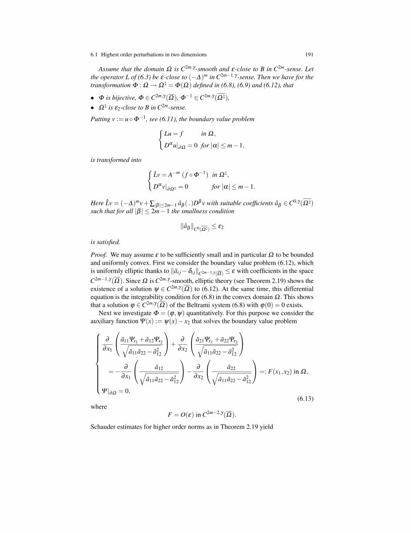
6.1 Highest order perturbations in two dimensions 191
Assume that the domain Ω is C2m,γ -smooth and ε-close to B in C2m-sense. Letthe operator L of (6.3) be ε-close to (−∆)m in C2m−1,γ -sense. Then we have for thetransformation Φ : Ω →Ω \ = Φ(Ω) defined in (6.8), (6.9) and (6.12), that
• Φ is bijective, Φ ∈C2m,γ(Ω), Φ−1 ∈C2m,γ(Ω \),• Ω \ is ε2-close to B in C2m-sense.
Putting v := uΦ−1, see (6.11), the boundary value problemLu = f in Ω ,
Dα u|∂Ω = 0 for |α| ≤ m−1,
is transformed into Lv = A−m ( f Φ
−1) in Ω \,
Dα v|∂Ω \ = 0 for |α| ≤ m−1.
Here Lv = (−∆)mv+∑|β |≤2m−1 aβ ( .)Dβ v with suitable coefficients aβ ∈C0,γ(Ω \)such that for all |β | ≤ 2m−1 the smallness condition
‖aβ‖C0(Ω \) ≤ ε2
is satisfied.
Proof. We may assume ε to be sufficiently small and in particular Ω to be boundedand uniformly convex. First we consider the boundary value problem (6.12), whichis uniformly elliptic thanks to ‖ai j−δi j‖C2m−1,γ (Ω) ≤ ε with coefficients in the spaceC2m−1,γ(Ω). Since Ω is C2m,γ -smooth, elliptic theory (see Theorem 2.19) shows theexistence of a solution ψ ∈ C2m,γ(Ω) to (6.12). At the same time, this differentialequation is the integrability condition for (6.8) in the convex domain Ω . This showsthat a solution ϕ ∈C2m,γ(Ω) of the Beltrami system (6.8) with ϕ(0) = 0 exists.
Next we investigate Φ = (ϕ,ψ) quantitatively. For this purpose we consider theauxiliary function Ψ(x) := ψ(x)− x2 that solves the boundary value problem
∂
∂x1
a11Ψx1 + a12Ψx2√a11a22− a2
12
+∂
∂x2
a21Ψx1 + a22Ψx2√a11a22− a2
12
=− ∂
∂x1
a12√a11a22− a2
12
− ∂
∂x2
a22√a11a22− a2
12
=: F(x1,x2) in Ω ,
Ψ |∂Ω = 0,(6.13)
whereF = O(ε) in C2m−2,γ(Ω).
Schauder estimates for higher order norms as in Theorem 2.19 yield
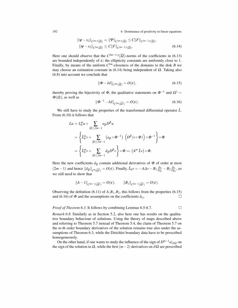
192 6 Dominance of positivity in linear equations
‖ψ− x2‖C2m,γ (Ω) = ‖Ψ‖C2m,γ (Ω) ≤C‖F‖C2m−2,γ (Ω),
‖ψ− x2‖C2m(Ω) ≤ C‖F‖C2m−2,γ (Ω). (6.14)
Here one should observe that the C2m−1,γ(Ω)-norms of the coefficients in (6.13)are bounded independently of ε; the ellipticity constants are uniformly close to 1.Finally, by means of the uniform C2m-closeness of the domains to the disk B wemay choose an estimation constant in (6.14) being independent of Ω . Taking also(6.8) into account we conclude that
‖Φ− Id‖C2m(Ω) = O(ε), (6.15)
thereby proving the bijectivity of Φ , the qualitative statements on Φ−1 and Ω \ =Φ(Ω), as well as
‖Φ−1− Id‖C2m(Ω \) = O(ε). (6.16)
We still have to study the properties of the transformed differential operator L.From (6.10) it follows that
Lu = Lm0 u+ ∑
|β |≤2m−1aβ Dβ u
=
Lm
0 v+ ∑|β |≤2m−1
(aβ Φ
−1) (Dβ (vΦ))Φ
−1
Φ
=
Lm
0 v+ ∑|β |≤2m−1
aβ Dβ v
Φ =:
(Am Lv
)Φ .
Here the new coefficients aβ contain additional derivatives of Φ of order at most(2m−1) and hence ‖aβ‖C0(Ω \) = O(ε). Finally, L0v =−A∆v−B1
∂v∂ξ1
−B2∂v
∂ξ2, so
we still need to show that
‖A−1‖C2m−2(Ω \) = O(ε), ‖B j‖C2m−2(Ω \) = O(ε).
Observing the definition (6.11) of A,B1,B2, this follows from the properties (6.15)and (6.16) of Φ and the assumptions on the coefficients ai j.
Proof of Theorem 6.3. It follows by combining Lemmas 6.5-6.7.
Remark 6.8. Similarly as in Section 5.2, also here one has results on the qualita-tive boundary behaviour of solutions. Using the theory of maps described aboveand referring to Theorem 5.7 instead of Theorem 5.4, the claim of Theorem 5.7 onthe m-th order boundary derivatives of the solution remains true also under the as-sumptions of Theorem 6.3, while the Dirichlet boundary data have to be prescribedhomogeneously.
On the other hand, if one wants to study the influence of the sign of Dm−1u|∂Ω onthe sign of the solution in Ω , while the first (m−2) derivatives on ∂Ω are prescribed
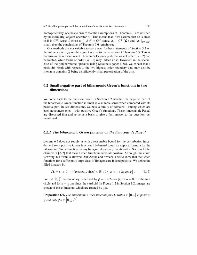
6.2 Small negative part of biharmonic Green’s functions in two dimensions 193
homogeneously, one has to ensure that the assumptions of Theorem 6.3 are satisfiedby the (formally) adjoint operator L∗. This means that if we assume that Ω is closeto B in C2m-sense, L close to (−∆)m in C2m-sense, aβ ∈ C|β |(Ω) and ‖aβ‖C|β |(Ω)small, then the conclusions of Theorem 5.6 remain true.
Our methods are not suitable to carry over further statements of Section 5.2 onthe influence of u|∂B on the sign of u in B to the situation of Theorem 6.3. This isbecause in the relevant result Theorem 5.15, only perturbations of order (m−2) canbe treated, while terms of order (m− 1) may indeed arise. However, in the specialcase of the polyharmonic operator, using Sassone’s paper [358], we expect that apositivity result with respect to the two highest order boundary data may also beshown in domains Ω being a sufficiently small perturbation of the disk.
6.2 Small negative part of biharmonic Green’s functions in twodimensions
We come back to the question raised in Section 1.2 whether the negative part ofthe biharmonic Green function is small in a suitable sense when compared with itspositive part. In two dimensions, we have a family of domains – among which areeven nonconvex ones – with positive Green’s functions. These limacons de Pascalare discussed first and serve as a basis to give a first answer to the question justmentioned.
6.2.1 The biharmonic Green function on the limacons de Pascal
Lemma 6.5 does not supply us with a reasonable bound for the perturbation in or-der to have a positive Green function. Hadamard found an explicit formula for thebiharmonic Green function on any limacon. As already mentioned in Section 1.2 heclaimed in [222] that these Green functions were all positive. Although this claimis wrong, his formula allowed Dall’Acqua and Sweers [120] to show that the Greenfunctions for a sufficiently large class of limacons are indeed positive. We define thefilled limacon by
Ωa = (−a,0)+(ρ cosϕ,ρ sinϕ) ∈ R2; 0≤ ρ < 1+2acosϕ
. (6.17)
For a ∈[0, 1
2
]the boundary is defined by ρ = 1 + 2acosϕ; for a = 0 it is the unit
circle and for a = 12 one finds the cardioid. In Figure 1.2 in Section 1.2, images are
shown of these limacons which are rotated by 12 π .
Proposition 6.9. The biharmonic Green function for Ωa with a ∈[0, 1
2
]is positive
if and only if a ∈[0, 1
6
√6].
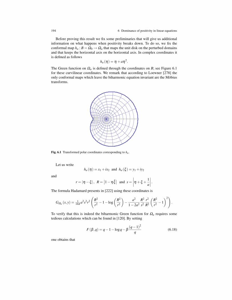
194 6 Dominance of positivity in linear equations
Before proving this result we fix some preliminaries that will give us additionalinformation on what happens when positivity breaks down. To do so, we fix theconformal map ha : B = Ω0 →Ωa that maps the unit disk on the perturbed domainsand that keeps the horizontal axis on the horizontal axis. In complex coordinates itis defined as follows
ha (η) = η +aη2.
The Green function on Ωa is defined through the coordinates on B; see Figure 6.1for these curvilinear coordinates. We remark that according to Loewner [278] theonly conformal maps which leave the biharmonic equation invariant are the Mobiustransforms.
Fig. 6.1 Transformed polar coordinates corresponding to ha.
Let us writeha (η) = x1 + ix2 and ha (ξ ) = y1 + iy2
and
r = |η−ξ | , R =∣∣1−ηξ
∣∣ and s =∣∣∣∣η +ξ +
1a
∣∣∣∣ .The formula Hadamard presents in [222] using these coordinates is
GΩa (x,y) = 116π
a2s2r2
(R2
r2 −1− log(
R2
r2
)− a2
1−2a2R2
s2r2
R2
(R2
r2 −1)2)
.
To verify that this is indeed the biharmonic Green function for Ωa requires sometedious calculations which can be found in [120]. By setting
F (β ,q) = q−1− logq−β(q−1)2
q(6.18)
one obtains that
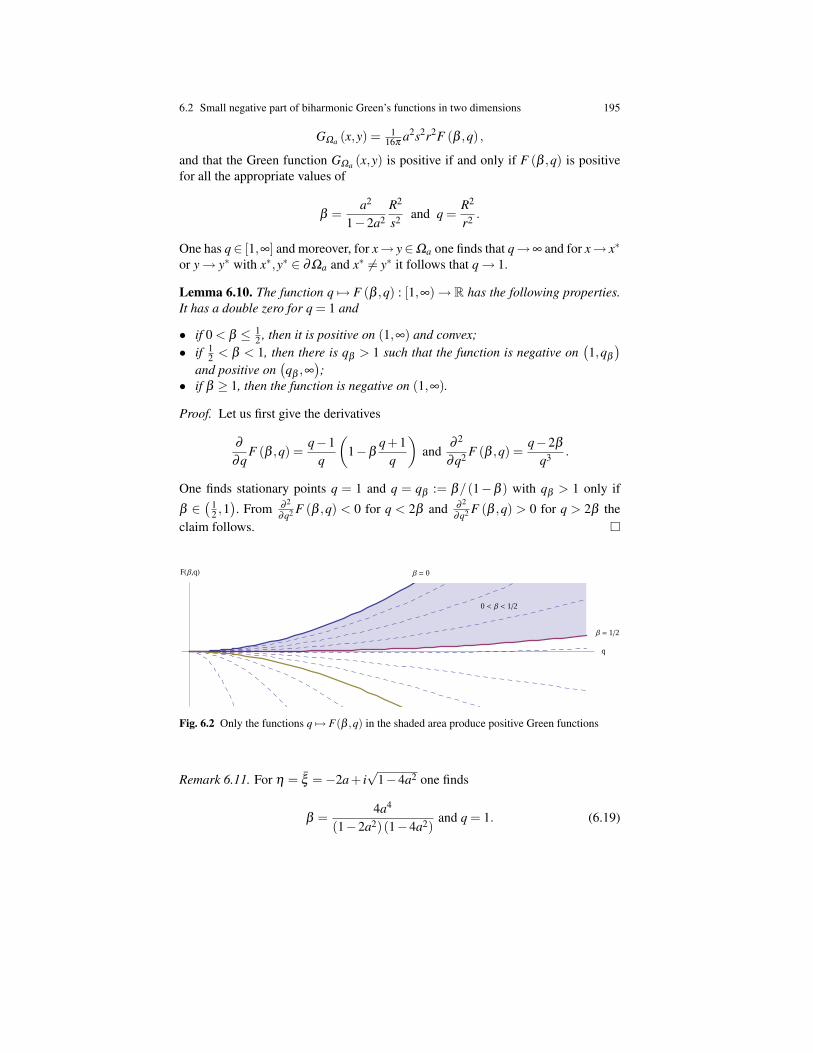
6.2 Small negative part of biharmonic Green’s functions in two dimensions 195
GΩa (x,y) = 116π
a2s2r2F (β ,q) ,
and that the Green function GΩa (x,y) is positive if and only if F (β ,q) is positivefor all the appropriate values of
β =a2
1−2a2R2
s2 and q =R2
r2 .
One has q∈ [1,∞] and moreover, for x→ y∈Ωa one finds that q→∞ and for x→ x∗
or y→ y∗ with x∗,y∗ ∈ ∂Ωa and x∗ 6= y∗ it follows that q→ 1.
Lemma 6.10. The function q 7→ F (β ,q) : [1,∞)→ R has the following properties.It has a double zero for q = 1 and
• if 0 < β ≤ 12 , then it is positive on (1,∞) and convex;
• if 12 < β < 1, then there is qβ > 1 such that the function is negative on
(1,qβ
)and positive on
(qβ ,∞
);
• if β ≥ 1, then the function is negative on (1,∞).
Proof. Let us first give the derivatives
∂
∂qF (β ,q) =
q−1q
(1−β
q+1q
)and
∂ 2
∂q2 F (β ,q) =q−2β
q3 .
One finds stationary points q = 1 and q = qβ := β/(1−β ) with qβ > 1 only if
β ∈( 1
2 ,1). From ∂ 2
∂q2 F (β ,q) < 0 for q < 2β and ∂ 2
∂q2 F (β ,q) > 0 for q > 2β theclaim follows.
0 < Β < 12
q
FH Β,qL Β = 0
Β = 12
Fig. 6.2 Only the functions q 7→ F(β ,q) in the shaded area produce positive Green functions
Remark 6.11. For η = ξ =−2a+ i√
1−4a2 one finds
β =4a4
(1−2a2)(1−4a2)and q = 1. (6.19)
196 6 Dominance of positivity in linear equations
Since β and q are continuous functions of η and ξ for ξ 6= η ∈ B, a necessarycondition for positivity is
4a4
(1−2a2)(1−4a2)≤ 1
2.
For a ∈[0, 1
2
]this last inequality is equivalent to a ∈
[0, 1
6
√6].
For a ∈ ( 16
√6,1/2] this disproves a claim by Hadamard [222], according to
which the clamped plate problem is positivity preserving for all limacons.
In order to find a positive Green function it is hence sufficient to show that β ≤ 12 ,
which is in its turn guaranteed when, for a ∈[0, 1
6
√6], the following holds for all
η ,ξ ∈ B:2a4 ∣∣1−ηξ
∣∣2 ≤ (1−2a2) |1+a(η +ξ )|2 .
Setting η1 = Reη , η2 = Imη and ξ1 = Reξ , η2 = Imη and 〈η ,ξ 〉 = η1ξ1 + η2ξ2,this condition can be rewritten as
β (η ,ξ )≤ 0, (6.20)
where β (η ,ξ ) is defined by
β (η ,ξ )
:= 2a4(
1+ |η |2)(
1+ |ξ |2)−((
1−2a2)(1+2a(η1 +ξ1))+a2 |η +ξ |2).
In order to show β ≤ 12 on B2 we may restrict ourselves to check (6.20) only for
certain pairs (η ,ξ ) ∈ B2. For the limacons the next lemma confirms the conjecturethat sign change under smooth perturbations of the domain starts from the boundary.
Lemma 6.12. Let η ,ξ ∈ B. It holds that β (η ,ξ )≤ β (χ, χ) for χ ∈ B satisfying
|χ| ≥max(|η | , |ξ |) and Reχ =12
Re(η +ξ ) .
Proof. The left term of (6.20) increases when η and ξ are replaced by χ and χ . Atthe same time the right term decreases since
|η +ξ |2 = (η1 +ξ1)2 +(η2 +ξ2)
2 ≥ (η1 +ξ1)2 = |χ + χ|2 .
Lemma 6.13. β(eiϕ ,e−iϕ
)≤ 1
2 for all ϕ ∈ [0,π] if and only if a ∈[0, 1
6
√6].
Proof. The inequality (6.20) with η = eiϕ and ξ = e−iϕ is equivalent to(1−2a2)(1+4acosϕ)+4a2 (cosϕ)2−8a4 ≥ 0.
6.2 Small negative part of biharmonic Green’s functions in two dimensions 197
The minimum of fa(t) =(1−2a2
)(1+4a t)+4a2t2−8a4 is assumed for
ta =1−2a2
−2a.
Only when a ∈[ 1
2
(√3−1
), 1
2
]one finds ta ≥ −1. Hence for a ∈
[0, 1
2
(√3−1
)]the function fa on [−1,1] has its minimum in −1 and(
1−2a2)(1+4acosϕ)+4a2 (cosϕ)2−8a4 ≥ (2a−1)2 (1−2a2)> 0.
For a ∈[ 1
2
(√3−1
), 1
2
]one finds that fa on [−1,1] has its minimum in ta:
min0≤ϕ≤π
(1−2a2)(1+4acosϕ)+4a2 (cosϕ)2−8a4 = fa (ta) = 2a2 (1−6a2) .
This last expression is positive if and only if a ∈[0, 1
6
√6].
Proof of Proposition 6.9. By Lemma 6.10 a necessary and sufficient condition forGΩa ( . , .) to be positive is β ≤ 1
2 , which is guaranteed by β ≤ 0. By Lemma 6.12one finds that it suffices to prove
supχ∈∂B
β (χ, χ)≤ 12.
The last step follows from Lemma 6.13.
6.2.2 Filling smooth domains with perturbed limacons
As mentioned before, the Green function for the biharmonic Dirichlet problem is ingeneral not positive. The few exceptions that we know can be classified as follows:
• Domains for which an explicit biharmonic Green function can be constructedand for which this Green function is positive. Typical examples are the limaconsof the previous section.
• Domains which are small perturbations, in the sense of Theorem 6.3, of a domainthat is known to have a positive biharmonic Green function with G satisfyingsimilar estimates as the Green function on the disk.
We have formulated this second class of domains more widely than just perturba-tions of the disk. Indeed, the proof of Theorem 6.3 can be copied starting with anylimacon Ωa as in (6.17) with a < 1
6
√6. One could even start with domains which
are images of those limacons under a Mobius mapping. Although here we only needMobius transforms in R2, we briefly discuss them in Rn. This shows that it is not a
198 6 Dominance of positivity in linear equations
lack of Mobius transforms which prevents us from extending the present reasoningto any space dimension.
Let us recall that every Mobius transformation φ of Rn can be written as
φ = φ1 j φ2
with j an inversion:j(x) = |x|−2 x
and φi a similarity:φi (x) = a+ c M x, (6.21)
where M is an orthogonal matrix, c a nonzero multiplication and a a shift. Theypossess the following property.
Lemma 6.14. Let φ be a Mobius transformation in Rn. Then
∆k(
J12−
kn
φuφ
)= J
12 + k
nφ
(∆
ku)φ
with Jφ =∣∣∣det
(∂φi∂x j
)∣∣∣, the modulus of the Jacobian determinant.
For a proof see for example [119]. Only due to the inversion the shape of adomain will change. This lemma allows one to pull back the Dirichlet biharmonicproblem from φ (Ωa) to Ωa and to use the Green function on Ωa for the problemon φ (Ωa). Of course, a Mobius transformed ball is still a ball. Examples of Mobiustransformed limacons can be seen in [119].
Having seen the relatively limited possibilities to have a positive Green function,one is curious to see how big the negative contribution of the Dirichlet biharmonicGreen function might be.
We will give a first and still preliminary answer to the following question whichwas raised already in Section 1.2 and which may be considered as an adequatereformulation of the Boggio-Hadamard conjecture:
Is positivity preserving in any bounded smooth domain Ω possibly “almost true” in thesense that the negative part G−
Ω(x,y) := max−GΩ (x,y),0 of the biharmonic Green func-
tion under Dirichlet boundary conditions is “small relatively” to the singular positive partG+
Ω(x,y) := maxGΩ (x,y),0?
In this section we will give an outline for the two-dimensional case, while for gen-eral dimensions, we refer to Section 6.4.
The main result is as follows.
Theorem 6.15. Let Ω ⊂ R2 be a bounded C4,γ -smooth domain and let GΩ denotethe biharmonic Green function in Ω under Dirichlet boundary conditions.
Then there exists a positive minimal distance δ = δ (Ω) > 0 such that for anytwo points x,y ∈Ω , x 6= y,
6.2 Small negative part of biharmonic Green’s functions in two dimensions 199
|x− y|< δ implies that GΩ (x,y) > 0. (6.22)
In particular, there exists a constant C = C(Ω) > 0 such that for all x,y ∈Ω , x 6= y,we have the following estimate from below:
GΩ (x,y)≥−C d(x)2 d(y)2. (6.23)
Remark 6.16. Together with the estimate from Theorem 4.28 (case |α| = |β | = 0)we obtain that with a constant C = C(Ω)
−C d(x)2 d(y)2 ≤ GΩ (x,y)≤C d(x)d(y)min
1,d(x)d(y)|x− y|2
.
Both estimates are sharp in general. For the lower bound we refer to Garabedian’sexample [176], while for the upper bound one may see Theorem 4.6. For x or ycloser to the boundary than to each other, the estimate from below is by a factor|x− y|2 smaller than the estimate from above.
The key step in proving Theorem 6.15 consists in decomposing the Green func-tion into a singular positive part modeled along sums of Green functions in suitablyperturbed limacons and a subordinate smooth possibly negative regular part.
Lemma 6.17. Assume that Ω ⊂ R2 is a bounded domain with ∂Ω ∈C4,γ . Then thebiharmonic Green function GΩ for (6.1) can be written as
GΩ (x,y) = GsingΩ
(x,y)+GregΩ
(x,y)
such that for some c2,c1 > 0:
0≤ GsingΩ
(x,y)≤ c1d(x)d(y)min
1,
d(x)d(y)|x− y|2
, (6.24)
and ∣∣GregΩ
(x,y)∣∣≤ c2d (x)2 d(y)2
for all (x,y) ∈Ω 2. Moreover:
1. GsingΩ
∈C1,γ(Ω 2)∩C1
0(Ω 2)∩C4,γ
(Ω 2\(x,x) ;x ∈Ω
)for all γ ∈ (0,1);
2. GregΩ∈C4,γ
(Ω 2)∩C1
0(Ω 2).
For a compact set K, the space C10(K) is defined to consist of all functions g∈C1(K)
satisfying g = |∇g|= 0 on ∂K.
The proof of this lemma is rather technical and lengthy. A detailed proof can befound in [117]. The main ingredients are first the positivity of the Green functionsfor the limacon and its ε-close C2,γ -perturbations, and secondly filling the domainfrom the interior with finitely many of those limacons. See Figure 6.3.
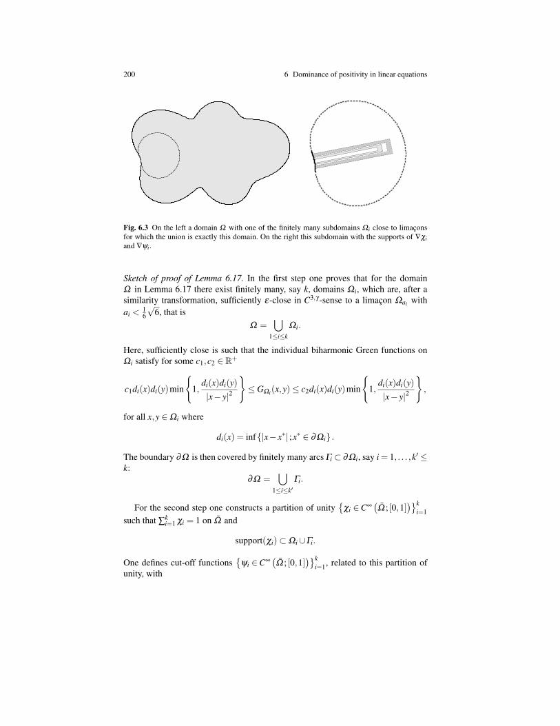
200 6 Dominance of positivity in linear equations
Fig. 6.3 On the left a domain Ω with one of the finitely many subdomains Ωi close to limaconsfor which the union is exactly this domain. On the right this subdomain with the supports of ∇χiand ∇ψi.
Sketch of proof of Lemma 6.17. In the first step one proves that for the domainΩ in Lemma 6.17 there exist finitely many, say k, domains Ωi, which are, after asimilarity transformation, sufficiently ε-close in C3,γ -sense to a limacon Ωai withai < 1
6
√6, that is
Ω =⋃
1≤i≤k
Ωi.
Here, sufficiently close is such that the individual biharmonic Green functions onΩi satisfy for some c1,c2 ∈ R+
c1di(x)di(y)min
1,
di(x)di(y)|x− y|2
≤ GΩi(x,y)≤ c2di(x)di(y)min
1,
di(x)di(y)|x− y|2
,
for all x,y ∈Ωi where
di(x) = inf|x− x∗| ;x∗ ∈ ∂Ωi .
The boundary ∂Ω is then covered by finitely many arcs Γi ⊂ ∂Ωi, say i = 1, . . . ,k′ ≤k:
∂Ω =⋃
1≤i≤k′Γi.
For the second step one constructs a partition of unity
χi ∈C∞(Ω ; [0,1]
)ki=1
such that ∑ki=1 χi = 1 on Ω and
support(χi)⊂Ωi∪Γi.
One defines cut-off functions
ψi ∈C∞(Ω ; [0,1]
)ki=1, related to this partition of
unity, with
6.2 Small negative part of biharmonic Green’s functions in two dimensions 201
support(ψi)⊂Ωi∪Γi
ψi(x) = 1 for x ∈ support(χi),support(∇ψi)∩ support(χi) = /0.
See Figure 6.3. Next, one defines
GsingΩ
(x,y) =k
∑i=1
ψi(x)GΩi(x,y)χi(y),
GregΩ
(x,y) = GΩ (x,y)−GsingΩ
(x,y),
with ψi(x)GΩi(x,y)χi(y) extended by 0 if x /∈Ωi or y /∈Ωi.Take some y ∈ Ω , keep it fixed in what follows and define Iy := i : y ∈
support(χi). Then
GsingΩ
(x,y) = ∑i∈Iy
ψi(x)GΩi(x,y)χi(y)
and one finds in distributional sense that
∆2Gsing
Ω(x,y) =
0 if x /∈
⋃i∈Iy support(ψi) =: AIy ,
δx(y) if x ∈⋃
i∈Iy support(χi) =: BIy ,∑i∈Iy ∆ 2
x(ψi(x)GΩi(x,y)
)χi(y) if x ∈ AIy\BIy .
(6.25)
Note that ∆ 2x(ψi(x)GΩi(x,y)
)χi(y) = 0 on
(AIy\BIy
)∩(AIy\support(∇ψi)
). In other
words, GsingΩ
takes care of the appropriate singularity at y and is positive throughthe construction that uses the GΩi . The support of Gsing
Ωlies in a band around the
diagonal (x,x) ; x ∈Ω. See Figure 6.4.For the biharmonic operator applied to the difference Greg
Ω(x,y) = GΩ (x,y)−
GsingΩ
(x,y) only the third term in (6.25) remains. Since ∆ 2GregΩ
(x,y) is zero nearthe diagonal (x,x) ;x ∈Ω it can be shown that Greg
Ωis a smooth as the boundary
allows:x 7→ ∑
i∈Iy
ψi(x)GΩi(x,y)χi(y) ∈C4,γ(
AIy\BIy
). (6.26)
The support of GregΩ
will in general be the full Ω × Ω .The estimates for Gsing
Ω(x,y) are inherited from those for GΩi(x,y); those for
GregΩ
(x,y) from the boundary conditions and (6.26).
Sketch of the proof of Theorem 6.15. By carefully checking the proof of Lemma 6.17one finds a rΩ > 0 and a positive constant c > 0 such that there is the followingestimate:
GsingΩ
(x,y)≥ cd(x)d(y)min
1,
d(x)d(y)|x− y|2
for |x− y|< rΩ .
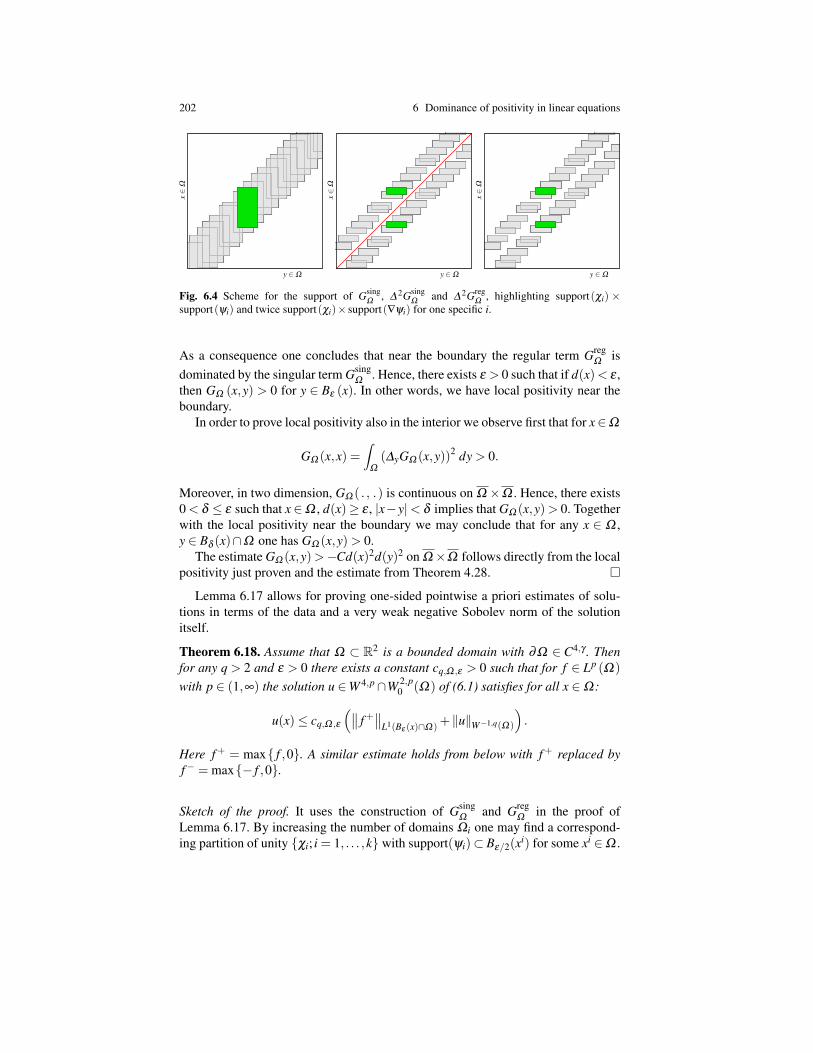
202 6 Dominance of positivity in linear equations
x∈
Ω
x∈
Ω
x∈
Ω
y ∈Ω y ∈Ω y ∈Ω
Fig. 6.4 Scheme for the support of GsingΩ
, ∆ 2GsingΩ
and ∆ 2GregΩ
, highlighting support(χi) ×support(ψi) and twice support(χi)× support(∇ψi) for one specific i.
As a consequence one concludes that near the boundary the regular term GregΩ
isdominated by the singular term Gsing
Ω. Hence, there exists ε > 0 such that if d(x) < ε ,
then GΩ (x,y) > 0 for y ∈ Bε (x). In other words, we have local positivity near theboundary.
In order to prove local positivity also in the interior we observe first that for x∈Ω
GΩ (x,x) =∫
Ω
(∆yGΩ (x,y))2 dy > 0.
Moreover, in two dimension, GΩ ( . , .) is continuous on Ω ×Ω . Hence, there exists0 < δ ≤ ε such that x∈Ω , d(x)≥ ε , |x−y|< δ implies that GΩ (x,y) > 0. Togetherwith the local positivity near the boundary we may conclude that for any x ∈ Ω ,y ∈ Bδ (x)∩Ω one has GΩ (x,y) > 0.
The estimate GΩ (x,y) >−Cd(x)2d(y)2 on Ω×Ω follows directly from the localpositivity just proven and the estimate from Theorem 4.28.
Lemma 6.17 allows for proving one-sided pointwise a priori estimates of solu-tions in terms of the data and a very weak negative Sobolev norm of the solutionitself.
Theorem 6.18. Assume that Ω ⊂ R2 is a bounded domain with ∂Ω ∈ C4,γ . Thenfor any q > 2 and ε > 0 there exists a constant cq,Ω ,ε > 0 such that for f ∈ Lp (Ω)with p ∈ (1,∞) the solution u ∈W 4,p∩W 2,p
0 (Ω) of (6.1) satisfies for all x ∈Ω :
u(x)≤ cq,Ω ,ε
(∥∥ f +∥∥L1(Bε (x)∩Ω) +‖u‖W−1,q(Ω)
).
Here f + = max f ,0. A similar estimate holds from below with f + replaced byf− = max− f ,0.
Sketch of the proof. It uses the construction of GsingΩ
and GregΩ
in the proof ofLemma 6.17. By increasing the number of domains Ωi one may find a correspond-ing partition of unity χi; i = 1, . . . ,k with support(ψi)⊂ Bε/2(xi) for some xi ∈Ω .
6.2 Small negative part of biharmonic Green’s functions in two dimensions 203
Setting
ui(x) =∫
Ωi
ψi(x)GΩi(x,y)χi(y) f (y)dy
and using the positivity of GΩi one finds ui(x) = 0 for x /∈ Bε/2(xi) and
ui(x) ≤∫
Bε/2(xi)∩Ωi
ψi(x)GΩi(x,y)χi(y) f +(y)dy
≤ c∥∥ f +∥∥
L1(Bε/2(xi)∩Ωi) ≤ c∥∥ f +∥∥
L1(Bε (x)∩Ωi)
when x ∈ Bε/2(xi). Since x ∈ support(ψi) for at most finitely many i’s, one obtains
using (x) :=k
∑i=1
ui(x) =∫
Ω
GsingΩ
(x,y) f (y)dy≤ c∥∥ f +∥∥
L1(Bε (x)∩Ω) .
The function u−using satisfies∣∣∣∆ 2(
u−using)
(x)∣∣∣= ∣∣∣∣ f (x)−∑
ki=1 ∆
2(
ψi(x)∫
Ωi
GΩi(x,y)χi(y) f (y)dy)∣∣∣∣
=∣∣∣∑k
i=1 ∑|α +β |= 4|α| ≥ 1
cα Dαψi(x)Dβ
∫Ωi
GΩi(x,y)χi(y) f (y)dy∣∣∣∣
≤ ∑ki=1 ∑
|α +β |= 4|α| ≥ 1
cα
∥∥∥∥Dαψi( .)Dβ
∫Ωi
GΩi( . ,y)χi(y) f (y)dy∥∥∥∥
L∞(support(∇ψi)).
By the Sobolev embedding W 1,q ⊂ L∞ for q > 2 and the properties of ψi it followsthat ∥∥∥∥Dα
ψi( .)Dβ
∫Ωi
GΩi( . ,y)χi(y) f (y)dy∥∥∥∥
L∞(support(∇ψi))
≤∥∥∥∥Dα
ψi( .)Dβ
∫Ωi
GΩi( . ,y)χi(y) f (y)dy∥∥∥∥
W 1,q0 (support(∇ψi))
=∥∥∥∥Dα
ψi( .)Dβ
∫Ωi
GΩi( . ,y)χi(y)(∆
2u)(y)dy
∥∥∥∥W 1,q
0 (support(∇ψi))
=∥∥∥∥Dα
ψi( .)Dβ
∫Ωi
∆2y(GΩi( . ,y)χi(y)
)u(y)dy
∥∥∥∥W 1,q
0 (support(∇ψi)). (6.27)
This last expression does not involve points (x,y) near the diagonal: support(χi)×support(∇ψi) is as in Figure 6.4 on the right. So (x,y) 7→Dα ψi(x)Dβ GΩi( . ,y)χi(y)is a C∞-function with compact support. It allows us to estimate (6.27) by a weaknorm of u like e.g. ‖u‖W−1,q(Ω). Elliptic Lp-estimates, see Section 2.5.2, and Sobolev
204 6 Dominance of positivity in linear equations
embeddings translate in several steps the L∞-bound for ∆ 2(u−using
)into an L∞-
bound for u−using.
6.3 Regions of positivity in arbitrary domains in higherdimensions
The remaining part of this chapter is mainly devoted to the biharmonic Green func-tion in dimensions
n≥ 3,
which corresponds to the Dirichlet problem∆
2u = f in Ω ,
u = |∇u|= 0 on ∂Ω .(6.28)
For brevity let GΩ := G∆ 2,Ω denote these Green functions in what follows.One goal will be to verify perturbation results like Theorem 6.3, another to prove
“smallness” of the negative part G−Ω
in general bounded smooth domains Ω ⊂ Rn
also if n ≥ 3, i.e. to extend Theorem 6.15 to higher dimensions. Our strategy toachieve the second goal is to identify subsets
P ⊂Ω ×Ω \(x,x)
where one can directly and explicitly verify that
GΩ (x,y) > 0 for all (x,y) ∈P.
Further steps to be done in Sections 6.4 and 6.5 will be a blow-up analysis and a dis-cussion of several limiting situations, which all together will imply also perturbationresults to achieve the first goal.
A first step to identify positivity sets P was done by Nehari [322] in dimensionsn = 2 and n = 3. Developing Nehari’s idea, in Section 6.3.1 we prove the followingresult.
Theorem 6.19. Let n≥ 3. Then there exists a constant δn > 0, which depends onlyon the dimension n, such that the following holds true.
Assume Ω ⊂ Rn to be a C4,γ -smooth bounded domain and let GΩ := G∆ 2,Ω
denote the Green function for the biharmonic operator under Dirichlet boundaryconditions. If
|x− y|< δn maxd(x),d(y),
then we haveGΩ (x,y) > 0.
For the constant δn, one may achieve that
6.3 Regions of positivity in arbitrary domains in higher dimensions 205
δ3 ≥ 4−2√
3≈ 0.53,
δ4 ≥ 0.59,
δn ≥ 0.6 for n≥ 5,
and
limn→∞
δn =√
5−12
≈ 0.618.
We recall that d(x) = dist(x,∂Ω). For two-dimensional domains, only a much morerestricted statement seems to be available, where also the maximal distance of x,yto boundary points of ∂Ω is involved, see [322].
By making use of d(x) ≤ d(y) + |x− y| one may observe that the condition|x− y|< δn maxd(x),d(y) implies that |x− y|< δn
1−δnmind(x),d(y).
The preceding theorem shows that the negative part of the Green function isuniformly bounded and hence relatively small compared with the singular positivepart, as long as x and y stay uniformly away from the boundary ∂Ω . It is remarkablethat the constant δn can be found independently of the domains Ω . In this form, theresult cannot be deduced from Schauder-type estimates.
With slightly more complicated but similar techniques as in the proof of Theo-rem 6.19, one may also cover the Green function for the Dirichlet problem G(−∆)m,Ω
for the polyharmonic operator. By means of the formula
u(x) =∫
Ω
G(−∆)m,Ω (x,y) f (y)dy
we find solutions of the polyharmonic Dirichlet problem(−∆)mu = f in Ω ,
Dα u|∂Ω = 0 for |α| ≤ m−1,(6.29)
provided f and Ω are smooth enough.In order to avoid distinctions and too many technicalities we prove in Sec-
tion 6.3.2 the following result only for large dimensions.
Theorem 6.20. Let m ∈ N+, n > 2m. Then there exists a constant δm,n > 0, whichdepends only on the dimension n and the order 2m of the polyharmonic operator,such that the following holds true.
Assume Ω ⊂ Rn to be a C2m,γ -smooth bounded domain and let G(−∆)m,Ω denotethe polyharmonic Green function under Dirichlet boundary conditions. If
|x− y|< δm,n maxd(x),d(y),
thenG(−∆)m,Ω (x,y) > 0.
For the constant δm,n, one may achieve that

206 6 Dominance of positivity in linear equations
δm,2m+1 ≥ 1+Γ (m)Γ
( 32
)Γ(m+ 1
2
) −√√√√1+
Γ (m)2Γ( 3
2
)2
Γ(m+ 1
2
)2
and, for fixed m, that
limn→∞
δm,n =√
5−12
≈ 0.618.
Remark 6.21. 1. A similar result was obtained for n = 2m by Kockritz in a seminarthesis [250]. Checking carefully the proof below indicates that it can be extendedto n≥ 2m−1 but will presumably fail for n≤ 2m−2.
2. Numerical evidence indicates the following for the constants δm,n.
• For each m the sequence (δm,n)∞n=2m+1 is increasing to
√5−12 .
• The sequence (δm,2m+1)∞m=2 is decreasing to 0.
• We provide lower bounds for δm,n, the limit of which for n → ∞ is√
5−12 ,
independently of m. The speed of convergence, however, seems to dependstrongly on m.
6.3.1 The biharmonic operator
In this section we prove Theorem 6.19. We consider the situation where, for someR > 1, we have
B := B1(0)⊂Ω ⊂ BR := BR(0)
and write, for suitable f : Rn → R,
GΩ f (x) :=∫
Ω
GΩ (x,y) f (y)dy
which yields the solution u(x) := GΩ f (x) to the Dirichlet problem (6.28).Let us recall that a fundamental solution for ∆ 2 on Rn is given by
Fn(x) =
cn|x|4−n if n 6∈ 2,4,
−2c4 log |x| if n = 4,
2c2|x|2 log |x| if n = 2,
where
cn =
1
2(n−4)(n−2)nenif n 6∈ 2,4,
18nen
if n ∈ 2,4.
6.3 Regions of positivity in arbitrary domains in higher dimensions 207
The Green function may be decomposed into the fundamental solution plus a regularpart
GΩ (x,y) = Fn(|x− y|)+HΩ (x,y),
where HΩ ∈C4,γ(
Ω2)
. We will also use
HΩ f (x) :=∫
Ω
HΩ (x,y) f (y)dy.
Lemma 6.22. Let f ,g be smooth and supported in B. Then
4∫
Ω
(∆GΩ f )(∆GΩ g) dx≥∫
B( f (HB f −HBR f )+g(HBg−HBR g)) dx
+∫
B( f (GBg+GBR g)+g(GB f +GBR f )) dx.
Proof. We consider the quadratic form
R2 3 (β ,γ) 7→∫
Ω
(β∆GΩ f + γ∆GΩ g)2 dx
and show that this is non-decreasing with respect to domain inclusion. For this pur-pose one considers ω ⊂Ω and one gets∫
Ω
(β∆GΩ f + γ∆GΩ g)2 dx−∫
ω
(β∆Gω f + γ∆Gω g)2 dx
=∫
Ω
(β∆GΩ f + γ∆GΩ g)2 dx+∫
ω
(β∆Gω f + γ∆Gω g)2 dx
−2∫
ω
(βGω f + γGω g)(β∆
2Gω f + γ∆2Gω g
)dx
=∫
Ω
(β∆GΩ f + γ∆GΩ g)2 dx+∫
ω
(β∆Gω f + γ∆Gω g)2 dx
−2∫
ω
(βGω f + γGω g)(β f + γg) dx
=∫
Ω
(β∆GΩ f + γ∆GΩ g)2 dx+∫
ω
(β∆Gω f + γ∆Gω g)2 dx
−2∫
ω
(βGω f + γGω g)(β∆
2GΩ f + γ∆2GΩ g
)dx
=∫
Ω
(β∆GΩ f + γ∆GΩ g)2 dx+∫
ω
(β∆Gω f + γ∆Gω g)2 dx
−2∫
ω
(β∆Gω f + γ∆Gω g)(β∆GΩ f + γ∆GΩ g) dx
=∫
Ω\ω
(β∆GΩ f + γ∆GΩ g)2 dx
+∫
ω
(β (∆GΩ f −∆Gω f )+ γ(∆GΩ g−∆Gω g))2 dx
≥ 0.
208 6 Dominance of positivity in linear equations
In a first step we exploit this monotonicity in B⊂Ω with β = γ = 1, that is∫Ω
(∆GΩ f +∆GΩ g)2 dx≥∫
B(∆GB f +∆GBg)2 dx =
∫B( f +g)GB ( f +g) dx.
(6.30)In a second step it is used in Ω ⊂ BR with β =−γ = 1, that is∫
Ω
(∆GΩ f −∆GΩ g)2 dx≤∫
BR
(∆GBR f −∆GBRg)2 dx =∫
B( f −g)GBR ( f −g) dx.
(6.31)Subtracting (6.31) from (6.30) yields
4∫
Ω
(∆GΩ f )(∆GΩ g) dx ≥∫
Bf (GB f −GBR f ) dx+
∫B
g(GBg−GBR g) dx
+∫
Bf (GBg+GBRg) dx+
∫B
g(GB f +GBR f ) dx.
Since GB−GBR = HB−HBR , the claim follows.
Lemma 6.23. For x,y ∈ B, x 6= y, we have the following estimate from below for thebiharmonic Green function of Ω ,
GΩ (x,y)≥ 14
(HB(x,x)−HBR(x,x)+HB(y,y)−HBR(y,y))
+12
(GB(x,y)+GBR(x,y)) .
Proof. The statement follows directly from Lemma 6.22 by taking smooth approxi-mations of the Dirac delta distribution concentrated in x and y respectively as f andg. One also uses the symmetry of the Green function GΩ (x,y) = GΩ (y,x).
Proof of Theorem 6.19. We recall from Lemma 2.27 that for n > 4 and n = 3,observing that c3 < 0,
GB(x,y) = cn
|x− y|4−n− n−2
2
∣∣∣∣|x|y− x|x|
∣∣∣∣4−n
+n−4
2
∣∣∣∣|x|y− x|x|
∣∣∣∣2−n
|x− y|2
,
(6.32)
GBR(x,y) = R4−nGB
(1R
x,1R
y)
,
HBR(x,x) =−cnn−2
2
(R− |x|2
R
)4−n
, (6.33)
while for n = 4
GB(x,y) = c4
−2log |x− y|+2log
∣∣∣∣|x|y− x|x|
∣∣∣∣−1+∣∣∣∣|x|y− x
|x|
∣∣∣∣−2
|x− y|2
,
(6.34)
6.3 Regions of positivity in arbitrary domains in higher dimensions 209
GBR(x,y) = GB
(1R
x,1R
y)
,
HBR(x,x) = 2c4 log(
1− |x|2
R2
)− c4 +2c4 logR. (6.35)
In order to prove Theorem 6.19, by rescaling and translation, it is enough to considerx = 0, y ∈ Bδn(0), where δn ∈ (0,1) has to be suitably specified below.
We consider first the case n > 4, where Lemma 6.23 and formulae (6.32)–(6.33)yield
4cn
GΩ (0,y) ≥ −n−22
+n−2
2R4−n− n−2
2(1−|y|2
)4−n+
n−22
(R− |y|2
R
)4−n
+ 4|y|4−n− (n−2)+(n−4)|y|2− (n−2)R4−n +(n−4)R2−n|y|2.
Letting R→ ∞, we obtain
4cn
GΩ (0,y)≥ 4|y|4−n +(n−4)|y|2− n−22(1−|y|2
)4−n− 32(n−2). (6.36)
If n = 5 one has to check whether
0 < 4−6|y|−4|y|2 +112|y|3−|y|5.
The right hand side is strictly decreasing in |y| ∈ [0,0.6] and takes on a positivevalue for |y|= 0.6. According to mapleTM the above inequality is satisfied for |y| ∈(0,0.612865 . . .).
If n ≥ 6, we drop the term (n− 4)|y|2 in (6.36) and have to determine δn suchthat
4δ4−nn − n−2
2(1−δ
2n)4−n− 3
2(n−2)≥ 0. (6.37)
Asymptotically, δn should be chosen close to the positive root δ∞ of
δ = 1−δ2,
i.e. to δ∞ = (√
5−1)/2. We show that (6.37) is satisfied with δn = 0.6, i.e. that
4(
35
)4−n
− n−22
(1625
)4−n
− 32(n−2)≥ 0
⇔ 8− (n−2)(
1516
)n−4
−3(n−2)(
35
)n−4
≥ 0.
The left hand side of the last expression is increasing for n≥ 18 and attains positivevalues for n = 6, . . . ,18, thereby showing that (6.37) holds true for δn = 0.6.
We discuss now the case n = 4 and choose R ≥ 1, where Lemma 6.23 and for-mulae (6.34)–(6.35) yield
210 6 Dominance of positivity in linear equations
2c4
GΩ (0,y) ≥ − log(
1− |y|2
R2
)+ log
(1−|y|2
)−2logR−4log |y|
+ 2logR−2+ |y|2 +|y|2
R2
≥ − log(
1− |y|2
R2
)+ log
(1−|y|2
)−4log |y|−2+ |y|2 +
|y|2
R2 .
Letting R→ ∞, we conclude that
2c4
GΩ (0,y)≥−4log |y|+ log(1−|y|2
)−2+ |y|2.
The right hand side is certainly decreasing in |y| ∈ [0,0.6] and takes a positive valuefor |y| = δ4 = 0.59. With the help of mapleTM we see that it is positive for |y| ∈(0,0.594160 . . .).
Finally, we discuss the case n = 3, where c3 = − 18π
< 0. Proceeding as beforewe find
− 2c3
GΩ (0,y) ≥ 14
(1−R+1−|y|2−R+
|y|2
R
)+(−2|y|+ 1
2+
R2
+(12
+1
2R)|y|2
)= 1−2|y|+ 1
4|y|2 +
34R|y|2.
Letting R→ ∞ yields
− 2c3
GΩ (0,y)≥ 1−2|y|+ 14|y|2,
where the right hand side is positive for |y|< 4−2√
3.
6.3.2 Extensions to polyharmonic operators
Here, we prove Theorem 6.20. The arguments are very similar to Section 6.3.1 andwe may be very brief and focus mainly on what is different. Throughout this section,according to Theorem 6.20, we confine ourselves to the case
n > 2m.
We considerB = B1(0)⊂Ω ⊂ BR = BR(0)
and the Green function G(−∆)m,Ω corresponding to (6.29) in Ω . Again, this Greenfunction may be decomposed into a singular and a regular part
6.3 Regions of positivity in arbitrary domains in higher dimensions 211
G(−∆)m,Ω (x,y) = cm,n|x− y|2m−n +H(−∆)m,Ω (x,y),
where H(−∆)m,Ω ∈ C2m,γ(Ω2) denotes the regular part and cm,n > 0 is a suitable
positive constant. Lemma 6.23 directly generalises to the polyharmonic situationand we may perform the
Proof of Theorem 6.20. According to Lemma 2.27 we have with a suitable positiveconstant km,n,
G(−∆)m,B(x,y) = km,n|x− y|2m−n∫ ∣∣∣|x|y− x
|x|
∣∣∣/|x−y|
1
(v2−1
)m−1v1−n dv, (6.38)
G(−∆)m,BR(x,y) = R2m−nG(−∆)m,B
(1R
x,1R
y)
, (6.39)
H(−∆)m,BR(x,x) = −km,n
n−2m
(R− |x|2
R
)2m−n
. (6.40)
The constants cm,n and km,n are related by
cm,n = km,n
∫∞
1
(v2−1
)m−1v1−n dv = km,n(−1)m
m−1
∑j=0
(−1) j(m−1
j
)2 j +2−n
= km,n2m−1(m−1)!
m
∏j=1
(n−2 j).
The latter identity is verified by induction.By the generalisation of Lemma 6.23, formulae (6.38)–(6.40) and letting R→∞,
we obtain
G(−∆)m,Ω (0,y) ≥ cm,n|y|2m−n−km,n
2|y|2m−n
∫∞
1/|y|
(v2−1
)m−1v1−n dv
−km,n
4(n−2m)
(1+(1−|y|2
)2m−n)
≥cm,n
2|y|2m−n−
km,n
4(n−2m)
(1+(1−|y|2
)2m−n)
(6.41)
so that
4(n−2m)km,n
G(−∆)m,Ω (0,y)≥ 2(m−1)!m−1
∏j=1
(n2− j) |y|2m−n−1−
(1−|y|2
)2m−n. (6.42)
Certainly, one finds δm,n > 0 such that the right hand side is positive for |y|< δm,n.For m fixed and n → ∞, the powers 2m− n dominate all the other terms and δm,n
212 6 Dominance of positivity in linear equations
may be chosen such that they approach, as in the biharmonic case, the positive zeroδ∞ of
δ = 1−δ2,
which is precisely√
5−12 . In the case n = 2m+1, (6.42) reads
4km,2m+1
G(−∆)m,Ω (0,y) ≥ 2Γ (m)Γ
( 32
)Γ(m+ 1
2
) 1|y|−1− 1
1−|y|2(6.43)
≥ 2Γ (m)Γ
( 32
)Γ(m+ 1
2
) 1|y|−1− 1
1−|y|. (6.44)
The right hand side (6.44) is positive if and only if
|y|< 1+Γ (m)Γ
( 32
)Γ(m+ 1
2
) −√√√√1+
Γ (m)2Γ( 3
2
)2
Γ(m+ 1
2
)2 . (6.45)
One might wonder whether dropping a positive term in (6.41) gives rise to a veryrough estimate. The previous estimate (6.45) would still allow for choosing δ2,5 =0.46, while the right hand side of (6.43) is positive for |y|< δ2,5 = 0.54. On the otherhand, according to Theorem 6.19, δ2,5 = 0.59 is admissible. This shows that one hasnot lost much in (6.41). In any case, our proof shows that we cannot do better thana constant δm,n with limm→∞ δm,2m+1 = 0, even if one had kept the second term in(6.41).
6.4 Small negative part of biharmonic Green’s functions inhigher dimensions
The goal of this section is to extend Theorem 6.15 to any dimension n≥ 2.
6.4.1 Bounds for the negative part
Theorem 6.24. Let Ω ⊂ Rn (n ≥ 2) be a bounded C4,γ -smooth domain. Let GΩ
denote the biharmonic Green function in Ω under Dirichlet boundary conditions.Then there exists a positive minimal distance δ = δ (Ω) > 0 such that for any
two points x,y ∈Ω , x 6= y,
|x− y|< δ implies that GΩ (x,y) > 0. (6.46)
In particular, there exists a constant C = C(Ω) > 0 such that for all x,y ∈Ω , x 6= y,we have the following estimate from below
6.4 Small negative part of biharmonic Green’s functions in higher dimensions 213
GΩ (x,y)≥−C d(x)2 d(y)2. (6.47)
For n = 2, the statement just recalls Theorem 6.15. The proof for the case n≥ 3will be given in Section 6.4.2.
Remark 6.25. So for any bounded C4,γ -smooth domain Ω ⊂ Rn there exists a con-stant C = C(Ω) > 0 such the biharmonic Green function GΩ satisfies the followingestimate:
−Cd(x)2d(y)2 ≤ GΩ (x,y)≤
C|x− y|4−n min
1,d(x)2d(y)2
|x− y|4
if n > 4,
C log(
1+d(x)2d(y)2
|x− y|4
)if n = 4,
Cd(x)2−n/2d(y)2−n/2 min
1,
d(x)n/2d(y)n/2
|x− y|n
if n = 2,3. (6.48)
The estimates from above follow from the two-sided estimates in Theorem 4.28.See also (4.8). Even for n = 2,3, where the Green function is bounded, the boundfrom below in 6.48 is a strong statement because in the case where x or y is closer tothe boundary than they are to each other, we gain a factor of order |x−y|n comparedwith the estimate in Theorem 4.28.
Remark 6.26. A functional analytic approach by Malyshev [283] shows for n = 2,3this estimate from below:
G∆ 2,Ω (x,y)≥−C(Ω)√
G∆ 2,Ω (x,x)G∆ 2,Ω (y,y) (6.49)
with a constant C(Ω) ∈ [0,1). Starting from (4.8) and using C(Ω) < 1 it followsthat the optimal constant for G∆ 2,Ω from below in (4.8) for x near y is smaller thanthe one from above. From (6.49) and (4.8) alone one does not get a qualitative betterestimate from below as in (6.48).
Since Theorem 6.24 in the case n = 2 is already proved by Theorem 6.15, werestrict ourselves in what follows to
n≥ 3.
And as we already mentioned, completely different techniques than for n = 2 haveto be used.
6.4.2 A blow-up procedure
The proof of Theorem 6.24 as well as the perturbation result Theorem 6.29 beloware deduced from the following statement that for smooth perturbations of a fixed
214 6 Dominance of positivity in linear equations
domain, pairs of interior zeros of the biharmonic Green functions cannot get arbi-trarily close to each other. Theorem 6.29 will extend Theorem 6.3 for the biharmonicoperator to dimensions n≥ 3 and will be proved below in Section 6.5.
Theorem 6.27. We assume that n ≥ 3 and that (Ωk) is a C4,γ -perturbation of thebounded C4,γ -smooth domain Ω according to Definition 4.19. Let Gk = G∆ 2,Ωk
de-note the biharmonic Green functions in Ωk under Dirichlet boundary conditions.Then there exists a positive number δ > 0, which is uniform for the whole family ofdomains, such that for all k ∈ N it holds that
x,y ∈Ωk, x 6= y, Gk(x,y) = 0 implies that |x− y| ≥ δ .
Proof. 1. The proof will be performed by contradiction making use of a rescalingor blow-up analysis which was developed by Grunau and Robert in [207].
After possibly passing to a subsequence, possibly replacing Ω with some fixedΩk0 and possibly relabeling the sequence we may assume by contradiction that
there exist xk,yk ∈Ωk, xk 6= yk, such that |xk− yk| → 0 and Gk(xk,yk) = 0. (6.50)
In view of local positivity – see Theorem 6.19 – there exists ρ > 0 such that
|xk− yk| ≥ ρ maxd(xk,∂Ωk),d(yk,∂Ωk). (6.51)
In particular, xk and yk are approaching the boundary ∂Ω . After possibly passing toa further subsequence we may assume that
there exists x∞ ∈ ∂Ω : xk,yk → x∞.
By means of a translation and rotation we may achieve that
x∞ = 0 and the first unit vector e1 is the exterior unit normal in x∞ = 0 of ∂Ω .
According to Definition 4.19 there exist C4,γ -diffeomorphisms Ψk : Ω → Ωk suchthat ‖Id−Ψk‖C4,γ (Ω) → 0. We introduce
x′k := Ψ−1
k (xk) ∈Ω , y′k := Ψ−1
k (yk) ∈Ω ,
where obviously x′k → 0, y′k → 0, |x′k−y′k| → 0 as k→∞. We introduce furthermorexk ∈ ∂Ω as the closest boundary point to x′k:
|x′k− xk|= d(x′k).
By virtue of x′k → 0 ∈ ∂Ω and the smoothness of ∂Ω , this is uniquely determinedfor k large enough and also satisfies xk → 0 for k → ∞.
2. For ξ ,η ∈ 1|x′k−y′k|
(−xk +Ω
)we introduce the following rescalings of the Green
functions Gk
6.4 Small negative part of biharmonic Green’s functions in higher dimensions 215
Gk(ξ ,η) := |x′k− y′k|n−4Gk(Ψk(xk + |x′k− y′k|ξ ),Ψk(xk + |x′k− y′k|η)).
The rescaled domains 1|x′k−y′k|
(−xk +Ω) approach the half space
H := x ∈ Rn : x1 < 0.
The goal is to prove that in a suitable sense (Gk) approaches the biharmonic Greenfunction G∆ 2,H , while from our assumption (6.50) we deduce some degenerate be-haviour of G∆ 2,H . In view of Boggio’s formula, the latter cannot occur and weobtain a contradiction.
First we see that the bounds from Theorem 4.20 yield uniformly in k, ξ and η∣∣Gk(ξ ,η)∣∣≤C|ξ −η |4−n, provided that n > 4. (6.52)
If n = 3,4 we conclude first that
∣∣∇Gk(ξ ,η)∣∣≤C
1 if n = 3,
|ξ −η |−1 if n = 4.
Upon integration we obtain that
∣∣Gk(ξ ,η)∣∣≤C
1+ |ξ |+ |η | if n = 3,
1+ | log |ξ −η ||+ log(1+ |ξ |+ |η |) if n = 4.(6.53)
We observe, defining
gk(ξ ) = Ψ∗
k (E )(xk + |x′k− y′k|ξ )
with the pulled back euclidean metric E in rescaled variables, that for any ξ ∈1
|x′k−y′k|(−xk +Ω
), we have in the sense of distributions
∆2gk,η
Gk(ξ , .) = δξ . (6.54)
This family of differential equations, the coefficients of which obey uniform bounds,together with the uniform bounds (6.52) and (6.53) allows to apply local interiorand boundary Schauder estimates (see Theorem 2.19). For each ξ ∈H we find afunction G(ξ , .) ∈ C4(H \ ξ) such that Gk(ξ , .) → G(ξ , .) in C4
loc(H \ ξ).Since Ψk → Id in C4 implies that gk(ξ ) → (δi j) locally uniformly in C3, this and(6.54) give in turn that for any ξ ∈H
∆2η G(ξ , .) = δξ
in the sense of distributions. Finally, in order to explain carefully the boundary con-ditions to be attained by G(ξ , .), we consider a suitable local C4,γ -smooth coordi-nate chart Φ for Ω near 0 with Φ(ξ ) = ξ + O(|ξ |2), which maps in particular aneighbourhood of 0 in ∂H onto a neighbourhood of 0 in ∂Ω . Defining
216 6 Dominance of positivity in linear equations
Φk(ξ ) :=1
|x′k− y′k|
(Φ
(Φ−1(xk)+ |x′k− y′k|ξ
)− xk
), (6.55)
we obtain local coordinate charts for 1|x′k−y′k|
(−xk +Ω) with the coordinates ξ in
bounded neighbourhoods of 0 in H . Since xk → 0 and Φ−1(xk) → 0, we haveuniformly for ξ in such sets and for k → ∞ that:
Φ
(Φ−1(xk)+ |x′k− y′k|ξ
)= Φ
(Φ−1(xk)
)+ |x′k− y′k|DΦ
(Φ−1(xk)
)ξ + O(|x′k− y′k|2 |ξ |2)
= xk + |x′k− y′k|ξ +o(1)|x′k− y′k| |ξ |+O(|x′k− y′k|2 |ξ |2)
with o(1) → 0 for k → ∞. This shows that Φk → Id locally uniformly. The chainrule directly yields also convergence of the derivatives so that we may conclude thatΦk → Id in C4
loc. This allows us to infer that
G(ξ ,η) = ∂η1G(ξ ,η) = 0mbox f orall ξ ∈H and all η ∈ ∂H .
Finally, (6.52) and (6.53) yield the following bounds for G (where ξ ,η ∈H , ξ 6=η)
|G(ξ ,η)| ≤C
1+ |ξ |+ |η | if n = 3,
1+ | log |ξ −η ||+ log(1+ |ξ |+ |η |) if n = 4,
|ξ −η |4−n if n≥ 5.
(6.56)
3. We prove that
G(ξ ,η) = G∆ 2,H (ξ ,η) for all ξ ,η ∈H such that ξ 6= η . (6.57)
To this end we keep ξ ∈ H fixed in what follows. As for the biharmonic Greenfunction in the half space we recall Boggio’s formula
G∆ 2,H (ξ ,η) =1
4nen|ξ −η |4−n
|ξ ∗−η |/|ξ−η |∫1
(v2−1)v1−n dv; (6.58)
where ξ ,η ∈ H , ξ ∗ = (−ξ1,ξ2, . . . ,ξn), see Lemma 2.27. We comment on theuniqueness issue of G∆ 2,H in dimensions n = 3,4 at the end of the present proof.
Both G(ξ , .) and G∆ 2,H (ξ , .) satisfy the biharmonic equation with the δ -distri-bution δξ as right hand side and zero Dirichlet boundary conditions on η1 = 0.We let ψ := ψξ := G(ξ , .)−G∆ 2,H (ξ , .). Hence, ψ ∈C∞
(H)
solves∆ 2ψ = 0 in H ,
ψ = ∂
∂η1ψ = 0 on η1 = 0. (6.59)
6.4 Small negative part of biharmonic Green’s functions in higher dimensions 217
Moreover, according to (6.56) and (6.58), for all η ∈H we have that
|ψ(η)| ≤C
1+ |η | if n = 3,
1+ | log |η | | if n = 4,
|η |4−n if n≥ 5;
(6.60)
|∇ψ(η)| ≤C
1 if n = 3,
|η |−1 if n = 4;(6.61)
where C = C(ξ ). According to [151, 232], writing η = (η2, . . . ,ηn),
ψ∗(η) :=
ψ(η) if η1 ≤ 0,
−ψ(−η1, η)−2η1∂
∂y1ψ(−η1, η)−η2
1 ∆ψ(−η1, η) if η1 > 0,
ψ∗ ∈C4 (Rn) is an entire biharmonic function. We consider now first the case n > 4.Below we will prove that (6.59) and (6.60) imply that also
|∇ jψ(η)| ≤C|η |4−n− j for all η ∈H and for j = 1,2, (6.62)
where C = C(ξ ). This immediately gives that |ψ∗(η)| ≤C|η |4−n and in particularthat ψ∗ is a bounded entire biharmonic function. Liouville’s theorem for biharmonicfunctions [323, p.19] yields that ψ∗(η)≡ 0 so that the claim of the lemma follows,provided n > 4.
If n = 3,4 we shall prove below that for j = 0,1,2 and for all η ∈H
|D2+ jψ(η)| ≤C|η |2−n− j, where C = C(ξ ). (6.63)
As above ψ∗ is an entire biharmonic function and so are Dψ∗ and D2ψ∗. We have|D2ψ∗(η)| ≤ C(1 + |η |)2−n and so, it follows that D2ψ∗(η) ≡ 0. In view of theboundary conditions in (6.59) we come up with ψ∗(η)≡ 0 also in the case n = 3,4.
It remains to prove (6.62) and (6.63). We consider first n > 4. Assume by contra-diction that there exists a sequence (η`) ⊂H such that |∇ jψ(η`)| |η`|n+ j−4 → ∞
for `→ ∞. Then, taking η`,1 as the first component of η`,
ψ`(η) := |η`|n−4ψ(η`−η`,1e1 + |η`|η
)would solve
∆ 2ψ` = 0 in H ,
ψ` = ∂
∂η1ψ` = 0 on η1 = 0.
From the assumption we conclude that∣∣∣∣∇ jψ`
(η`,1
|η`|e1
)∣∣∣∣= |η`|n+ j−4|∇ jψ(η`)| → ∞. (6.64)
218 6 Dominance of positivity in linear equations
On the other hand,
|ψ`(η)| ≤C|η`|n−4 ∣∣η`−η`,1e1 + |η`|η∣∣4−n ≤C
∣∣∣∣ η`
|η`|+η−
η`,1
|η`|e1
∣∣∣∣4−n
, (6.65)
so that ψ` remains bounded in a neighbourhood of η`,1|η`|
e1 in H . Local Schauderestimates (see Theorem 2.19) yield∣∣∣∣∇ j
ψ`
(η`,1
|η`|e1
)∣∣∣∣≤C,
thereby contradicting (6.64). This proves (6.62).As for (6.63), i.e. in particular n = 3,4, the proof is quite similar since we can al-
ready make use of the gradient estimates (6.61). Instead of (6.65) one has to employ
|∇ψ`(η)| ≤C|η`|n−3 ∣∣η`−η`,1e1 + |η`|η∣∣3−n ≤C
∣∣∣∣ η`
|η`|+η−
η`,1
|η`|e1
∣∣∣∣3−n
,
so that ∇ψ` remains bounded uniformly outside η`|η`|
− η`,1|η`|
e1. Therefore, since ψ`
vanishes on ∂H , we get that ψ` is bounded in a neighbourhood of η`,1|η`|
e1 in H .The proof of (6.57) is complete.4. From assumption (6.50) we obtain
Gk
(x′k− xk
|x′k− y′k|,
y′k− xk
|x′k− y′k|
)= 0. (6.66)
Since x′k−xk|x′k−y′k|
,y′k−xk|x′k−y′k|
are bounded by virtue of |x′k − xk| = d(x′k) and boundedness
of d(x′k)/|x′k− y′k| according to (6.51), we may assume after possibly passing to afurther subsequence that
there exist ξ0,η0 ∈H :x′k− xk
|x′k− y′k|→ ξ0,
y′k− xk
|x′k− y′k|→ η0.
Observe that |ξ0 −η0| = 1. We recall from (6.55) the construction of local C4,γ -smooth coordinate charts ξ 7→ Φk(ξ ) for 1
|x′k−y′k|(−xk +Ω) with coordinates ξ in
bounded neighbourhoods of 0 in H . These converge in C4loc to the identity. Instead
of Gk we consider Gk := Gk (Φk,Φk) in H ×H \ ξ = η. As in Step 2 ofthis proof, elliptic theory (see Theorem 2.19) yields that Gk → G∆ 2,H in C4((H ∩B1/2(ξ0))×(H ∩B1/2(η0))). Exploiting this convergence, the boundary data of theGreen functions and using Taylor’s expansion we conclude from (6.66) that one ofthe following three possibilities occurs
1. ξ0 ∈H , η0 ∈H , G∆ 2,H (ξ0,η0) = 0;2. ξ0 ∈H , η0 ∈ ∂H , ∆η G∆ 2,H (ξ0,η0) = 0, or vice versa;3. ξ0 ∈ ∂H , η0 ∈ ∂H , ∆ξ ∆η G∆ 2,H (ξ0,η0) = 0.
6.5 Domain perturbations in higher dimensions 219
From Boggio’s formula (6.58) for the biharmonic Green function G∆ 2,H in the halfspace H , it follows by direct calculation that
for all ξ ,η ∈H such that x 6= y : G∆ 2,H (ξ ,η) > 0;for all ξ ∈H ,η ∈ ∂H : ∆η G∆ 2,H (ξ ,η) > 0;for all x,y ∈ ∂H , x 6= y : ∆ξ ∆η G∆ 2,H (ξ ,η) > 0.
This shows that none of the possibilities mentioned above may occur. Hence wehave achieved a contradiction and the theorem is proved.
Remark 6.28. The arguments in Step 3 of the previous proof show that if n = 3,4, the“boundary conditions” at infinity |G∆ 2,H (x,y)| ≤C (1 + |x|+ |y|) yield a uniquelydetermined biharmonic Green function in H .
Finally, basing upon Theorem 6.27 it is straightforward to prove Theorem 6.24.
Proof of Theorem 6.24. In order to prove (6.46) we assume by contradictionthat there exist sequences (xk),(yk) ⊂ Ω , xk 6= yk such that GΩ (xk,yk) ≤ 0 andlimk→∞ |xk− yk| = 0. In view of the smoothness assumptions made on Ω one mayconstruct sequences (ξk),(ηk) ⊂ Ω , ξk 6= ηk such that GΩ (ξk,ηk) = 0 as well aslimk→∞ |ξk−ηk|= 0. Application of Theorem 6.27 with all Ωk ≡Ω directly yieldsa contradiction.
Formula (6.47) now follows from (6.46) and Theorem 4.28.
6.5 Domain perturbations in higher dimensions
In Section 6.1 we studied the question whether the positivity of the biharmonicGreen function in the two-dimensional (unit) disk remains under sufficiently smallsmooth domain perturbations. Here, we prove the same result in dimensions n≥ 3.For domain closeness we refer to Definition 6.1.
Theorem 6.29. Let B be the unit ball of Rn, n≥ 2. Then there exists ε0 = ε0(n) > 0such that for ε ∈ [0,ε0] the following holds true.
Assume that Ω ⊂Rn is a C4,γ -smooth domain which is ε-close to the ball B in theC4,γ -sense. Then the Green function G∆ 2,Ω for ∆ 2 in Ω under Dirichlet boundaryconditions is strictly positive, that is
G∆ 2,Ω (x,y) > 0 for all x,y ∈Ω , x 6= y.
The proof given in Section 6.1 for the case n = 2 is direct and explicit, basedon perturbation series, Green’s function estimates and conformal maps. This meansthat in principle ε0 there may be calculated explicitly. Moreover, in the case n = 2,
220 6 Dominance of positivity in linear equations
according to the observation by Sassone [358], closeness has to be assumed only ina weaker norm.
In what follows, again, we restrict ourselves to considering
n≥ 3.
In this case, the proof is somehow more indirect since a number of proofs by con-tradiction are involved so that it will be impossible to calculate ε0 for n≥ 3 from theproofs.
Recalling Remark 6.4 we emphasise once more that Theorem 6.29 is by no meansjust a continuous dependence on data result.
Under suitable assumptions on the dimension n, the same techniques will allowfor proving a result like Theorem 6.29 also for polyharmonic operators (−∆)m.Presumably one will have to require the condition n≥ 2m−1 on the dimension, seeRemark 6.21.
The proof of Theorem 6.29 for n ≥ 3 will basically follow from the next resultwhich describes in which way the transition from positivity to sign change mayoccur within a smooth family of domains, see Definition 4.19.
Theorem 6.30. We assume that n ≥ 3 and that (Ωk) is a C4,γ -perturbation of thebounded C4,γ -smooth domain Ω . Let Gk = G∆ 2,Ωk
and G = G∆ 2,Ω denote the bihar-monic Green functions in Ωk and Ω respectively under Dirichlet boundary condi-tions.
We suppose that there exist two sequences (xk),(yk) such that xk,yk ∈Ωk and
xk 6= yk, Gk(xk,yk) = 0 for all k ∈ N.
Up to a subsequence, let x∞ := limk→+∞ xk and y∞ := limk→+∞ yk. Then x∞,y∞ ∈Ω ,x∞ 6= y∞ and we are in one of the following situations
• if x∞,y∞ ∈Ω , then G(x∞,y∞) = 0;• if x∞ ∈Ω and y∞ ∈ ∂Ω , then ∆yG(x∞,y∞) = 0;• if x∞ ∈ ∂Ω and y∞ ∈Ω , then ∆xG(x∞,y∞) = 0;• if x∞,y∞ ∈ ∂Ω , then ∆x∆yG(x∞,y∞) = 0.
Proof. The crucial statement is that x∞ 6= y∞, which already follows from Theo-rem 6.27. In view of the smoothness and convergence properties of the Green func-tions Gk,G, which are proved in Section 4.4, the claim follows directly from theassumption Gk(xk,yk) = 0 by means of Taylor’s expansion.
Theorem 6.29 now follows with a simple proof by contradiction since in theunit ball B ⊂ Rn Boggio’s formula (2.65) shows that none of the above mentioneddegeneracies may indeed occur.
Lemma 6.31. The biharmonic Green function in B = B1(0)⊂Rn, which is given by
6.6 Bibliographical notes 221
G∆ 2,B(x,y) =1
4nen|x− y|4−n
∣∣∣|x|y− x|x|
∣∣∣/|x−y|∫1
(v2−1)v1−n dv (x,y ∈ B, x 6= y)
enjoys the following properties
for all x,y ∈ B, x 6= y : G∆ 2,B(x,y) > 0;for all x ∈ B,y ∈ ∂B : ∆yG∆ 2,B(x,y) > 0;for all x,y ∈ ∂B, x 6= y : ∆x∆yG∆ 2,B(x,y) > 0.
Proof. These properties are verified by explicit calculations.
6.6 Bibliographical notes
The presentation of the perturbation theory of positivity and smallness of the nega-tive parts is based on [117, 120, 204, 206, 207, 208, 214]. The results in Section 6.1were first proved in [208], while the exposition is adapted from [204]. Section 6.2outlines and develops results by Dall’Acqua, Meister, and Sweers which originallyappeared in [117, 120]. The presentation of Section 6.3 follows [214]. The materialin Sections 6.4 and 6.5 is based on [206, 207], which are joint works of Grunau andRobert.
In two dimensions, the required notion of domain closeness to have positivityas in Theorem 6.3 was relaxed by Sassone [358]. Local positivity was consideredfirst by Nehari [322] for the clamped plate equation in dimensions n = 2,3, whereTheorem 6.19 was proved for n = 3 and a restrictive version of it for n = 2. A firstmathematical indication that the negative part of biharmonic Green’s functions issmaller than their positive part was obtained by Malyshev [283] by means of a func-tional analytic approach. There, the estimate from below uses the same expressionsas from above but with a smaller constant while we use smaller expressions anddo not discuss the magnitude of the constants. Hedenmalm, Jakobsson, and Shi-morin [225, 226] exhibit further examples of fourth order operators with a positiveGreen function and outline a strategy how to reduce the positivity discussion ofGreen’s functions to that of suitable Poisson kernels. This approach supports thefeeling that when transition from positivity to sign change occurs, this will happenmost likely via the last variant in Theorem 6.30. Corresponding results for bound-ary value problems for fourth order ordinary differential equations were achievedby Schroder [363, 364, 365].
Further contributions to the Boggio-Hadamard conjecture are discussed in detailin Section 1.2. One may also see [225, 226, 283, 294].

Chapter 7Semilinear problems
We study the elliptic polyharmonic reaction-diffusion-type model equation
(−∆)mu = f (u) (7.1)
in bounded domains Ω ⊂ Rn and in most cases together with Dirichlet boundaryconditions
Dα u|∂Ω = 0 for |α| ≤ m−1. (7.2)
These boundary conditions prevent (7.1) from being written as a system of sec-ond order boundary value problems. However, in some cases, also (homogeneous)Navier boundary conditions (2.21) or Steklov boundary conditions (2.22) may beparticularly interesting. We assume that the nonlinearity f : R → R is continuousand, in most cases, non-decreasing. The latter condition will be crucial in provingexistence and further properties of positive solutions. A large part of this chapterwill be devoted to special superlinear nonlinearities of polynomial growth such as
f (u) = λu+ |u|p−1u, p > 1, (7.3)
where λ ∈ R is a parameter.As was pointed out in Section 1.5, problem (7.1)-(7.3) with m = 2 and p = n+4
n−4may be considered as prototype for the Paneitz equation from fourth order confor-mal geometry. We come back to this geometrical issue in Section 7.10. However, themain focus of the present chapter is different. In higher order equations no generalmaximum principle is available (see Section 1.2), and truncation methods are notadmissible. Therefore, many well established techniques from second order equa-tions fail. One goal is to study the model problem (7.1)-(7.2) in order to establishsome new and general techniques which may be useful also in other situations andwhich may outline future developments. A second goal is to find out, in how far itis still possible to show qualitative properties of solutions in spite of the lack of amaximum principle.
If m = 1 and Ω = B is the unit ball, a celebrated result by Gidas-Ni-Nirenberg[195] states radial symmetry of positive solutions to (7.1)-(7.2) under mild smooth-
223
224 7 Semilinear problems
ness assumptions on the nonlinearity f . The proof is strongly based on the useof maximum principles and reflection methods. In Section 7.1 we explain how tosubstitute these by kernel estimates and monotonicity properties of the biharmonicGreen function. Only an additional sign and a monotonicity condition have to beimposed on f in order to enable us to extend the result to all m≥ 1.
Concerning existence and nonexistence of nontrivial solutions of the Dirichletproblem (7.1)-(7.2)-(7.3) the results strongly depend – as in the case m = 1 of sec-ond order equations – on the value of the exponent p. In order to avoid technicaldistinctions we assume that n > 2m in what follows. To explain the meaning of“critical growth” we start with the observation that (7.1)-(7.2)-(7.3) may be consid-ered – at least formally – as Euler-Lagrange equations of the functional
Eλ (v) :=
12∫
Ω
(∆ kv)2 dx− λ
2∫
Ωv2 dx− 1
p+1∫
Ω|v|p+1 dx if m = 2k is even,
12∫
Ω
∣∣∇∆ kv∣∣2 dx− λ
2∫
Ωv2 dx− 1
p+1∫
Ω|v|p+1 dx if m = 2k +1 is odd.
(7.4)The highest order term forces us to work in the space Hm
0 (Ω). Thanks to the em-bedding
Hm0 (Ω)⊂ Ls+1(Ω), s =
n+2mn−2m
, n > 2m,
the functional (7.4) is well-defined for p ≤ s and enjoys compactness properties ifp < s. The latter so-called subcritical case is relatively simple and in Section 7.2 weshow for any λ ∈ R the existence of infinitely many solutions.
The situation is completely different and much more difficult in the critical casewhere p = s, which is the case of geometrical relevance. This issue reflects theconformal covariance property of the Paneitz operator. The polyharmonic modelproblem at critical growth reads as follows,
(−∆)mu = λu+ |u|s−1u, u 6≡ 0 in Ω ,Dα u|∂Ω = 0 for |α| ≤ m−1
and is studied in detail in Sections 7.4 to 7.9 also under different boundary con-ditions. A first systematical investigation of the partial loss of compactness and –more generally – the compactness properties of variational functionals with criticalgrowth is due to Struwe [380] when m = 1. In Section 7.9.5 we prove an extensionof his result to the present case, namely m = 2.
In the supercritical regime p > s (n > 2m), the variational formulation (7.4)breaks down completely. Instead, in Section 7.11 different techniques like a super-subsolution method or – in the case of radial solutions – dynamical systems tech-niques have to be developed and are applied to study the slightly different modelproblem
∆2u = λ (1+u)p, u > 0 in B,
u = |∇u|= 0 on ∂B,
7.1 A Gidas-Ni-Nirenberg type symmetry result 225
where p > (n+4)/(n−4) and n > 4. Although similar results may be expected alsofor the analogous polyharmonic problem, technical difficulties prevent us here fromdeveloping this issue further.
7.1 A Gidas-Ni-Nirenberg type symmetry result
In this section we extend the symmetry result by Gidas-Ni-Nirenberg [195], whichholds for m = 1, to higher order elliptic problems with m ≥ 2. We consider bothDirichlet and Navier boundary conditions. Let us start with the first case.
Theorem 7.1. Assume that f : [0,∞)→ R is a continuous, non-decreasing functionwith f (0)≥ 0 and that u ∈Hm
0 ∩L∞(B) is a nonnegative nontrivial weak solution tothe Dirichlet problem
(−∆)mu = f (u) in B,
Dα u|∂B = 0 for |α| ≤ m−1.(7.5)
Then u is radially symmetric and strictly decreasing in the radial variable.
By elliptic regularity (see Theorem 2.20) we readily infer that a bounded weaksolution u to (7.5) satisfies u ∈C2m−1,γ(B), see also Lemma 7.5 below. Moreover, iff is smooth, Theorem 2.19 shows that u ∈C2m(B) is a classical solution of (7.5). Infact, u is even more regular. From Boggio’s formula it is immediate that u > 0 in B.
The proof of Theorem 7.1 is given as follows. In Section 7.1.1 we establish someinequalities for the polyharmonic Green function relative to Dirichlet boundary con-ditions and its derivatives. In Section 7.1.2 we carry out the moving plane procedureon the corresponding integral equation and complete the proof of Theorem 7.1.
Remark 7.2. 1. The monotonicity assumption on f crucially enters the proof. Ifwe assume instead that f is differentiable and satisfies for every s ≥ 0 thatf ′(s) < Λm,1 := first Dirichlet eigenvalue of (−∆)m, then (7.5) admits at mostone weak solution which is then necessarily radially symmetric. Indeed, assum-ing by contradiction that u,v ∈Hm
0 ∩L∞(B) are different weak solutions of (7.5),we find
(u− v,u− v)Hm0
=∫
B( f (u)− f (v))(u− v)dx < Λm,1
∫B(u− v)2 dx
contrary to the variational characterisation of Λm,1. Here, we used the scalarproduct defined in (2.10). In fact, symmetry is also ensured if f ′(s) : s ∈ Rdoes not contain any nonradial Dirichlet eigenvalue of (−∆)m (see [269]) or iff ′(s) < Λm,2 (see [124]). Uniqueness is guaranteed for sublinear f (see [127]).
2. An inspection of the proof shows that Theorem 7.1 is also valid for (7.5) withf (u) replaced by the nonautonomous radial nonlinearity f (|x|,u) provided thatf : [0,1]× [0,∞)→ [0,∞) is continuous, non-increasing in the first variable and
226 7 Semilinear problems
non-decreasing in the second one. If f is increasing in the first variable, the state-ment may become false, see [45, Theorem 3].
On the other hand, as long as Navier boundary conditions are involved, the scalarequation (7.1) may be rewritten as a system of m equations and the classical movingplane procedure applies. In this respect, the following statement is a direct conse-quence of a result by Troy [396].
Theorem 7.3. Assume that f : [0,∞) → R is a continuously differentiable, non-decreasing function with f (0) ≥ 0 and that u ∈ Hm ∩L∞(B) is a nonnegative non-trivial weak solution to the Navier problem
(−∆)mu = f (u) in B,
∆ ju|∂B = 0 for j = 0, . . . ,m−1.
Then the maps r 7→ (−∆)ku(r) are radially symmetric and strictly decreasing forall k = 0, . . . ,m−1.
We point out that under the assumptions of Theorem 7.3, the solution u satisfiesu ∈C2m(B), see Theorem 2.19.
The following example shows that the sign assumption on f , in both Theorems7.1 and 7.3, is necessary in order to have the monotonicity of positive radial solu-tions.
Example 7.4. Let J0 and I0 denote respectively the Bessel function and the so-calledmodified Bessel function of the first kind. Some computations show that the function
v(r):= i(
J0
(e
14 πir)− I0
(e
14 πir))
= i∞
∑k=0
(− 1
4 e12 πir2
)k
(k!)2 −
(14 e
12 πir2
)k
(k!)2
=∞
∑k=0
2(−1)k
((2k +1)!)2
( r2
)4k+2
solves ∆ 2v =−v in R2 and oscillates with increasing amplitude.Let r0 > 0 denote the first nonzero minimum of v and let m0 = −v(r0) > 0.
Numerically one finds that r0 = 8.28 . . . and m0 = 72.33 . . . . Putting u0(r) = v(r)+m0 and f (u) = m0−u, one finds that u0 > 0 satisfies
∆ 2u0 = f (u0) in Br0 ,u0 = |∇u0|= 0 on ∂Br0 ,
(7.6)
but the radially symmetric solution u0 is not decreasing, see Figure 7.1.
Now let r1 > 0 denote the first zero of ∆v(r) = v′′(r)+v′(r)/r. Define the numberm1 =−v(r1) > 0. Numerically one finds r1 = 7.23 . . . and m1 = 50.15 . . . . By settingu1 (r) = v(r)+m1 and f (u) = m1−u one finds that u1 > 0 satisfies
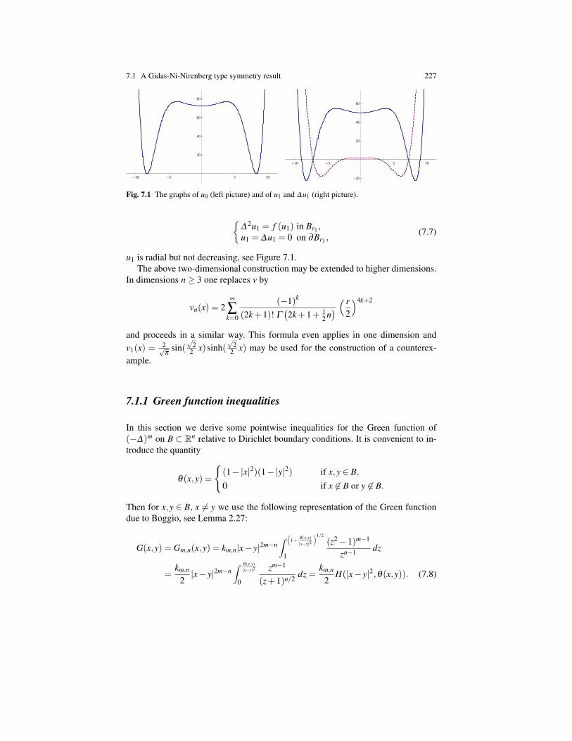
7.1 A Gidas-Ni-Nirenberg type symmetry result 227
-10 -5 5 10
20
40
60
80
-10 -5 5 10
-20
20
40
60
Fig. 7.1 The graphs of u0 (left picture) and of u1 and ∆u1 (right picture).
∆ 2u1 = f (u1) in Br1 ,u1 = ∆u1 = 0 on ∂Br1 ,
(7.7)
u1 is radial but not decreasing, see Figure 7.1.The above two-dimensional construction may be extended to higher dimensions.
In dimensions n≥ 3 one replaces v by
vn(x) = 2∞
∑k=0
(−1)k
(2k +1)! Γ(2k +1+ 1
2 n) ( r
2
)4k+2
and proceeds in a similar way. This formula even applies in one dimension andv1(x) = 2√
πsin(
√2
2 x)sinh(√
22 x) may be used for the construction of a counterex-
ample.
7.1.1 Green function inequalities
In this section we derive some pointwise inequalities for the Green function of(−∆)m on B ⊂ Rn relative to Dirichlet boundary conditions. It is convenient to in-troduce the quantity
θ(x,y) =
(1−|x|2)(1−|y|2) if x,y ∈ B,
0 if x 6∈ B or y 6∈ B.
Then for x,y ∈ B, x 6= y we use the following representation of the Green functiondue to Boggio, see Lemma 2.27:
G(x,y) = Gm,n(x,y) = km,n|x− y|2m−n∫ (
1+ θ(x,y)|x−y|2
)1/2
1
(z2−1)m−1
zn−1 dz
=km,n
2|x− y|2m−n
∫ θ(x,y)|x−y|2
0
zm−1
(z+1)n/2 dz =km,n
2H(|x− y|2,θ(x,y)). (7.8)
228 7 Semilinear problems
Here km,n is the positive constant from Lemma 2.27 and
H : (0,∞)× [0,∞)→ R, H(s, t) = sm− n2
∫ ts
0
zm−1
(z+1)n/2 dz. (7.9)
The following lemma is a direct consequence of formula (7.8), elliptic regularity(see Section 2.5.2) and the estimates in Chapter 4.
Lemma 7.5. Let h ∈ L∞(B), and let u ∈ Hm0 (B) satisfy
(u,v)Hm0
=∫
Bhvdx for all v ∈ Hm
0 (B),
i.e., u is a weak solution of (−∆)mu = h in B under Dirichlet boundary conditions.Then u ∈C2m−1,γ(B), and u satisfies
Dα u(x) =∫
BDα
x G(x,y)h(y)dy for every x ∈ B,
where Dα stands for any partial derivative of order |α|< 2m. In particular, Dα u≡ 0on ∂B for |α| ≤ m−1.
We need the following inequalities for the derivatives of the function H definedin (7.9).
Lemma 7.6. For all s, t > 0 we have
Hs(s, t) < 0, Ht(s, t) > 0, Hst(s, t) < 0.
Proof. We have
Ht(s, t) =tm−1
(t + s)n/2 , Hst(s, t) =− ntm−1
2(t + s)n/2+1
and
Hs(s, t) = (m− n2)sm− n
2−1∫ t
s
0
zm−1
(z+1)n/2 dz− tm
s(t + s)n/2 .
Hence the last two inequalities follow. Also the first inequality follows in case n ≥2m while in the remaining case n < 2m, we rewrite Hs(s, t) as
Hs(s, t) = (m− n2)∫ t
0
xm−1
s(x+ s)n/2 dx− tm
s(t + s)n/2
= (m− n2)∫ t
0
xm− n2−1
s
(x
x+ s
)n/2
dx− tm
s(t + s)n/2
< (m− n2)(
tt + s
)n/2 ∫ t
0
xm− n2−1
sdx− tm
s(t + s)n/2 = 0.
7.1 A Gidas-Ni-Nirenberg type symmetry result 229
This completes the proof.
In the following, we assume that G is trivially extended to Rn×Rn \(x,x); x ∈Rn, i.e., G(x,y) = 0 if |x| ≥ 1 or |y| ≥ 1. Then formula (7.8) is valid for all x,y∈Rn,x 6= y. We introduce some more notation. For all λ ∈ [0,1] we put
Tλ := x = (x1, . . . ,xn) ∈ Rn; x1 = λ and Σλ := x = (x1, . . . ,xn) ∈ B; x1 < λ.(7.10)
Moreover, for any x ∈ Rn let x denote its reflection about Tλ .
Lemma 7.7. Let λ ∈ [0,1). Then for every x ∈ B∩Tλ and y ∈ Σλ we have
Gx1(x,y) < 0 and (7.11)Gx1(x,y)+Gx1(x,y)≤ 0. (7.12)
Moreover, the second inequality is strict if λ > 0.
Proof. For abbreviation, we put d := |x− y|2 = |x− y|2 > 0, θ = θ(x,y) > 0, andθ = θ(x,y)≥ 0. Then
Gx1(x,y) = km,n
(Hs(d,θ)(x1− y1)−Ht(d,θ)(1−|y|2)x1
)< 0,
by Lemma 7.6, since x1 ≥ 0 and x1 > y1. Moreover
Gx1(x,y)+Gx1(x,y) = km,n
(Hs(d,θ)(x1− y1)+Hs(d,θ)(x1− (y)1)
)−km,n
([Ht(d,θ)(1−|y|2)+Ht(d,θ)(1−|y|2)]x1
)≤ km,n[Hs(d,θ)−Hs(d,θ)](x1− y1), (7.13)
where we used Lemma 7.6 and the fact that x1−y1 = y1−x1. Since moreover θ ≤ θ
and Hst < 0 in (0,∞)2 by Lemma 7.6, we conclude that Hs(d,θ)−Hs(d,θ) ≤ 0.Hence, (7.12) follows from (7.13). Finally, if λ > 0, then we have the strict inequal-ity θ < θ , so that we obtain a strict inequality in (7.13).
Lemma 7.8. Let λ ∈ (0,1). For all x,y ∈ Σλ , x 6= y, we have
G(x,y) > maxG(x,y),G(x,y), (7.14)G(x,y)−G(x,y) > |G(x,y)−G(x,y)|. (7.15)
Proof. Concerning (7.14), it suffices to prove G(x,y) > G(x,y) due to symmetryand to consider the case y ∈ B. We first observe that
|x− y|= |x− y|< |x− y|= |x− y|. (7.16)
Moreover, since |x|> |x|, |y|> |y|, we have that
θ(x,y) > maxθ(x,y),θ(x,y) ≥minθ(x,y),θ(x,y)> θ(x,y) (7.17)
230 7 Semilinear problems
and may conclude that
G(x,y) =km,n
2H(|x− y|2,θ(x,y)
)>
km,n
2H(|x− y|2,θ(x,y)
)>
km,n
2H(|x− y|2,θ(x,y)
)= G(x,y).
Here we used that H is strictly decreasing in the first argument and increasing in thesecond one, see Lemma 7.6.
In view of (7.14), in order to prove (7.15) we may restrict ourselves to x,y ∈ Band observe first that (7.15) is equivalent to
H(|x− y|2,θ(x,y)
)−H
(|x− y|2,θ(x,y)
)>∣∣H (|x− y|2,θ(x,y)
)−H
(|x− y|2,θ(x,y)
)∣∣ .This means that, in view of (7.16) and (7.17), we have to show that
0 < s1 < s2, 0 < t1 < t2 < t4, 0 < t1 < t3 < t4⇒ H(s1, t4)−H(s1, t1) > |H(s2, t2)−H(s2, t3)| .
Indeed, the latter follows again from Lemma 7.6 since
H(s1, t4)−H(s1, t1) =∫ t4
t1Ht(s1, t)dt >
∫ t4
t1Ht(s2, t)dt
>∫ maxt2,t3
mint2,t3Ht(s2, t)dt = |H(s2, t2)−H(s2, t3)| .
This completes the proof.
7.1.2 The moving plane argument
In this section we complete the proof of Theorem 7.1. Consider a fixed nonnegativenontrivial weak solution u ∈ Hm
0 ∩ L∞(B) of (7.5). From Corollary 2.21 we knowthat u ∈C2m−1,γ(B), see also Proposition 7.15 below. Hence, from Lemma 2.27 weknow that u > 0 in B, see also Theorem 3.6 for a direct statement without regularity.Let Tλ , Σλ and x be defined as in (7.10). We first provide some crucial estimatesfor directional derivatives which are related to the Hopf boundary lemma for secondorder problems. We recall the following statement as a special case of Theorem 5.7.
Lemma 7.9. If x0 ∈ ∂B and µ is a unit vector with µ · x0 < 0, then∂ mu∂ µm (x0) > 0.
In the following we extend u by zero outside of B so that it is defined on thewhole of Rn and we put
7.1 A Gidas-Ni-Nirenberg type symmetry result 231
f (s) =
f (s) if s > 00 if s = 0 (7.18)
so that f : [0,∞)→ [0,∞) is still non-decreasing while it may lose continuity at s = 0.For the next estimate we need the following technical result.
Lemma 7.10. Let 0 < λ < 1, and suppose that u(x) ≥ u(x) for all x ∈ Σλ . Thenf (u(y))≥ f (u(y))≥ 0 for all y∈ Σλ , and there exists a nonempty open set Oλ ⊂ Σλ
such that f (u(y)) > f (u(y)) or f (u(y)) > 0 for all y ∈Oλ .
Proof. The inequalities f (u(y))≥ f (u(y))≥ 0 for all y∈ Σλ follow from the mono-tonicity and positivity assumption on f . For the second statement it then sufficesto show that f (u(y)) 6≡ 0 in Σλ since then one of the two above inequalities wouldbecome strict in a nonempty open set Oλ ⊂ Σλ . By contradiction, if f (u) ≡ 0 inΣλ then the above inequalities would imply f (u) ≡ 0 in B. In turn, this implies(−∆)mu≡ 0 which contradicts the positivity of u.
Thanks to the above lemmas we obtain a statement on the sign of ∂u∂x1
.
Lemma 7.11. Let 0 < λ < 1, and suppose that u(x) ≥ u(x) for all x ∈ Σλ . Thenthere exists γ ∈ (0,λ ) such that ∂u
∂x1< 0 on T`∩B for all ` ∈ (λ − γ,λ ).
Proof. By Lemma 7.5, for all x ∈ Tλ ∩B we have
∂u∂x1
(x) =∫
BGx1(x,y) f (u(y))dy =
∫Σλ
(Gx1(x,y) f (u(y))+Gx1(x,y) f (u(y))
)dy.
(7.19)According to Lemma 7.10 we have f (u(y)) ≥ f (u(y)) ≥ 0 for all y ∈ Σλ and twocases may occur. In the first case, f (u(y)) > f (u(y)) for all y ∈ Oλ ; in this case,(7.19) yields
∂u∂x1
(x) <∫
Σλ
(Gx1(x,y)+Gx1(x,y)) f (u(y))dy≤ 0 for all x ∈ Tλ ∩B,
where in the first inequality we used (7.11) and in the second we used (7.12). In thesecond case, f (u(y)) > 0 for all y ∈Oλ ; in this case,
∂u∂x1
(x)≤∫
Σλ
(Gx1(x,y)+Gx1(x,y)) f (u(y))dy < 0 for all x ∈ Tλ ∩B,
where in the first inequality we used (7.12) which is strict for λ > 0. In any case,
∂u∂x1
(x) < 0 for all x ∈ Tλ ∩B. (7.20)
For any y ∈ Rn and any a > 0 consider now the cube centered at y, namely
Ua(y) :=
x ∈ Rn; max1≤i≤n
|xi− yi|< a
.
232 7 Semilinear problems
In view of Lemma 7.9, for any x0 ∈ Tλ ∩∂B we know that
(−1)m(
∂
∂x1
)m−1∂u∂x1
(x0) =(− ∂
∂x1
)m
u(x0) > 0 .
Since from the boundary conditions we also know that ( ∂
∂x1)ku(x0) = 0 for all k =
0, . . . ,m−1, there exists a = a(x0) > 0 such that
∂u∂x1
(x) < 0 for all x ∈Ua(x0)∩B. (7.21)
Then by the compactness of Tλ ∩∂B there exists a > 0 such that
∂u∂x1
(x) < 0 for all x ∈ A :=⋃
x0∈Tλ∩∂B
(Ua(x0)∩B) . (7.22)
Consider now the compact set K := (Tλ ∩ B) \ A and for d > 0 consider Kd :=K−de1. In view of (7.20), there exists δ > 0 such that
∂u∂x1
< 0 on Kd for all d ∈ [0,δ ]. (7.23)
Let γ := mina,δ> 0. Then the statement follows from (7.22)-(7.23).
We are now ready to start the moving plane procedure by shifting the plane Tλ
from the initial tangent position T1 towards the interior of B.
Lemma 7.12. There exists ε > 0 such that for all λ ∈ [1− ε,1) we have
u(x) > u(x) for x ∈ Σλ ,∂u∂x1
(x) < 0 for x ∈ Tλ ∩B. (7.24)
Proof. Note that T1∩∂B = e1, where e1 = (1,0, . . . ,0). By arguing as for (7.21),we infer that there exists ε > 0 such that ∂u
∂x1(x) < 0 for x ∈ B\Σ1−2ε . In turn, from
this we infer that (7.24) holds for all λ ∈ [1− ε,1).
Next we make sure that we can move the plane until we reach the origin.
Lemma 7.13. We have
Λ :=
λ ∈ (0,1); u(x) > u(x) ∀x ∈ Σλ ,∂u∂x1
(x) < 0 ∀x ∈ Tλ ∩B
= (0,1).
Proof. By Lemma 7.12 we know that [1− ε,1)⊂Λ . Let λ ∈ [0,1) be the smallestnumber such that (λ ,1)⊂Λ ; the proof will be complete once we show that λ = 0.By continuity we have
u(x)≥ u(x) for all x ∈ Σλ. (7.25)

7.1 A Gidas-Ni-Nirenberg type symmetry result 233
By contradiction assume that λ > 0. Then by Lemma 7.11 and (7.25) we infer that
there exists γ ∈ (0, λ ) such that∂u∂x1
< 0 on T`∩B for all ` ∈ (λ − γ, λ ).(7.26)
Consider the function f defined in (7.18). For all x ∈ Σλ
we compute
u(x)−u(x) =∫
B(G(x,y)−G(x,y)) f (u(y))dy (7.27)
=∫
Σλ
(G(x,y)−G(x,y)) f (u(y))dy+∫
Σλ
(G(x,y)−G(x,y)) f (u(y))dy .
According to Lemma 7.10, two cases may occur. If f (u(y)) > f (u(y)) for ally ∈Oλ , then (7.14) and (7.27) yield
u(x)−u(x) >∫
Σλ
(G(x,y)−G(x,y)+G(x,y)−G(x,y)) f (u(y))dy≥ 0,
where the last inequality follows from (7.15). If f (u(y)) > 0 for all y ∈ Oλ , thenagain (7.14), (7.15) and (7.27) yield
u(x)−u(x)≥∫
Σλ
(G(x,y)−G(x,y)+G(x,y)−G(x,y)) f (u(y))dy > 0 .
Hence we have shown in any case that
u(x) > u(x) for all x ∈ Σλ. (7.28)
From (7.26) and (7.28) we deduce by a standard compactness argument that thereexists 0 < γ1 < γ such that
u(x) > u(x) for all x ∈ Σ` and ` ∈ (λ − γ1, λ ].
This, combined with (7.26), shows that (λ − γ1, λ ] ⊂ Λ , contrary to the characteri-sation of λ .
Now we complete the proof of Theorem 7.1. Since 0 ∈ ∂Λ by Lemma 7.13, thecontinuity of u implies that
u(−x1,x2, . . . ,xn)≥ u(x1,x2, . . . ,xn) for x = (x1, . . . ,xn) ∈ B with x1 ≥ 0. (7.29)
Since, for a given rotation A ∈ SO(n), the function uA := u A is also a positiveweak solution of (7.5), inequality (7.29) also holds for uA in place of u. This readilyimplies that u is symmetric with respect to every hyperplane containing the origin.Consequently, u is radially symmetric. Moreover, we have ∂u
∂ r < 0 in B\0, since∂u∂x1
< 0 in x ∈ B, x1 > 0 by definition of Λ .
234 7 Semilinear problems
7.2 A brief overview of subcritical problems
In this section we briefly show how existence results for higher order semilinearsubcritical problems exhibit no surprises when compared with second order prob-lems. On the other hand, positivity of particular solutions (such as mountain-passsolutions) is not ensured in general domains. We start with some important factsconcerning the regularity of the solution.
7.2.1 Regularity for at most critical growth problems
Let Ω ⊂ Rn be a bounded domain and consider the equation
(−∆)mu = λu+ |u|p−1u in Ω , (7.30)
where λ ∈ R and 1 < p≤ s = n+2m
n−2m if n > 2m,1 < p < ∞ if n≤ 2m.
(7.31)
These equations are called at most critical with respect to the space Hm(Ω) dueto the upper bound for p, which coincides with the critical Sobolev exponent s. Wecomplement (7.30) with homogeneous boundary conditions of different kinds. Wemainly focus our attention on the Dirichlet boundary conditions
Dα u|∂Ω = 0 for |α| ≤ m−1, (7.32)
but we will also consider Navier boundary conditions
∆ju|∂Ω = 0 for j ≤ m−1, (7.33)
or, when m = 2, Steklov boundary conditions
u|∂Ω = (∆u−auν)|∂Ω = 0 (a ∈ R). (7.34)
Before going through existence and nonexistence results, we should clarify what ismeant by a solution for each one of these problems. For the Navier problem, thesuitable space
Hmϑ (Ω) =
v ∈ Hm(Ω); ∆
jv = 0 on ∂Ω for j < 12 m
(7.35)
was defined in (2.35) which, thanks to elliptic estimates, is a Hilbert space whenendowed with the following scalar product and corresponding norm
(u,v)Hmϑ
=
∫Ω
∆ ku∆ kv if m = 2k,∫Ω
∇(∆ ku) ·∇(∆ kv) if m = 2k +1,‖u‖Hm
ϑ= (u,u)1/2
Hmϑ
. (7.36)

7.2 A brief overview of subcritical problems 235
Note that H2ϑ(Ω) = H2 ∩H1
0 (Ω), the space which is needed for Steklov boundaryconditions. Recalling the definition of solution in the linear case, see (2.42), it isnatural to give the following definition.
Definition 7.14. Assume (7.31).
1. Let ( . , .)Hm0
denote the bilinear form in (2.10). We say that u ∈Hm0 (Ω) is a weak
solution to (7.30)-(7.32) if
(u,v)Hm0
=∫
Ω
(λu+ |u|p−1u)vdx for all v ∈ Hm0 (Ω).
2. We say that u ∈ Hmϑ
(Ω) is a weak solution to (7.30)-(7.33) if
(u,v)Hmϑ
=∫
Ω
(λu+ |u|p−1u)vdx for all v ∈ Hmϑ (Ω).
3. We say that u ∈ H2∩H10 (Ω) is a weak solution to (7.30)-(7.34) if∫
Ω
∆u∆vdx =∫
Ω
(λu+ |u|p−1u)vdx+a∫
∂Ω
uν vν dω for all v ∈ H2∩H10 (Ω).
Thanks to the at most criticality assumption (7.31), all the above definitions makesense. This definition should also be compared with (2.42) which holds for linearproblems. Moreover, we refer to the discussion following Theorem 2.15 to find anexplanation of how these weak formulations “contain” the boundary conditions.
Once existence of a solution (according to the previous definition) is established,one would like to find out if it has some regularity properties. The answer shows adeep difference between at most critical and supercritical problems. Let us explainthis crucial fact with a simple example. In a bounded C2m,γ -domain Ω , consider(7.30) with λ = 0 and complemented with Dirichlet boundary conditions
(−∆)mu = |u|p−1u in Ω ,Dα u|∂Ω = 0 for |α| ≤ m−1.
(7.37)
Assume first that p < s. Then, if u∈Hm0 (Ω) is a weak solution to (7.37), by Theorem
2.4 we know that u ∈ Ls+1(Ω) so that the right hand side f (u) = |u|p−1u of (7.37)belongs to L(s+1)/p(Ω). Therefore, Theorem 2.20 implies that u ∈W 2m,(s+1)/p(Ω).In turn, a further application of Theorem 2.4 shows that u∈ Ln(s+1)/(np−2ms−2m)(Ω).Since p < s we have n(s+1)
np−2ms−2m > s+1 so that we have gained some summability ofu and f (u). By repeating a finite number of times the same combination of Theorems2.20 and 2.4, we arrive at u ∈ W 2m,q(Ω) for some q > n
2m . Hence, Theorem 2.6applies and we infer that f (u) ∈ C0,γ(Ω) for some γ > 0. Finally, Theorem 2.19implies that u ∈C2m,γ(Ω) and that u is a classical solution to (7.37).
The same arguments apply to more general semilinear equations such as
(−∆)mu = g(u)

236 7 Semilinear problems
with g ∈ C1(R), |g(s)| ≤ c(1 + |s|p) for all s ∈ R and for some p < s and c > 0.Moreover, one can replace Dirichlet boundary conditions (7.32) with (7.33), (7.34),or any other set of boundary conditions which satisfy the complementing condition,see Definition 2.9.
On the other hand, this procedure fails if p > s. To see this, let n ≥ 3, let p >2(n−1)
n−2 and consider the second order problem−∆u = λ (1+u)p in B,u = 0 on ∂B,
(7.38)
with λ = 2p−2 (n−2− 2
p−2 ) > 0. Some computations allow to verify that the function
u(x) = |x|−2/(p−2)− 1 solves (7.38) in B \ 0. Moreover, u is a weak solution to(7.38) in H1
0 (B), if and only if p > s = n+2n−2 . However, u is not a classical solution
since u 6∈ L∞(B). We study in some detail supercritical biharmonic equations like(7.38) in Section 7.11.
This striking difference between the two cases p < s and p > s is one of the rea-sons why p = s is called the critical exponent with respect to the space Hm. In fact,the above described bootstrap argument also fails for p = s since, in this case, thereis no gain of regularity after an application of Theorems 2.20 and 2.4. However, withsome different and more involved arguments, Luckhaus [281] was able to prove theoptimal regularity result also for the critical growth case. By restricting our attentionto the problem treated in this chapter, we quote the following general result.
Proposition 7.15. Assume that Ω ⊂ Rn is a bounded domain and that (7.31) holds.Let u be a weak solution to one of the above problems. Then u is an analytic func-tion in x ∈ Ω ; u(x) 6= 0. Moreover, if ∂Ω ∈C2m,γ , then u ∈C2m,γ(Ω) and u is aclassical solution.
Proof. We refer to Luckhaus [281] for the general statement under Dirichlet bound-ary conditions (7.32). For Navier boundary conditions (7.33), the problem may betreated as a system, see [399, Appendix B] for the details in the case m = 2. Thesame arguments apply also to Steklov boundary conditions (7.34), see [42, Proposi-tion 23]. The function u 7→ λu + |u|p−1u is analytic for u 6= 0 so that the solution uis analytic in x ∈Ω ; u(x) 6= 0 in view of [312, 313].
Additional regularity (such as in Ck,γ for k > 2m) can be obtained, provided onetakes into account the regularity of the nonlinearity s 7→ |s|p−1s in a neighbourhoodof s = 0.
Remark 7.16. Since variational methods are involved, the boundary ∂Ω needs notbe smooth if one is merely interested in existence results for (7.30). In general,solutions only enjoy local smoothness properties. If one wishes to have global reg-ularity results, Proposition 7.15 tells us that the solution inherits smoothness fromthe boundary provided p ≤ s. Global regularity is quite important because, whenp = s, the Pohozaev identity (see Section 7.4 below) shows nonexistence of smoothsolutions in certain domains, and in order to have complementary existence results,it appears convenient to consider smooth solutions.
7.2 A brief overview of subcritical problems 237
We conclude this section by emphasising a further difference between (strictly)subcritical problems and critical problems. In the case of reaction-type model non-linearities f (u) as in (7.30), the possibility of finding a priori estimates seems to belimited to the (strictly) subcritical case p < s, see [126, 352, 375] and, for secondorder equations, the fundamental contribution [196] of Gidas and Spruck. On theother hand, in the critical regime branches of solutions to (7.30) may blow up for λ
in bounded intervals, see e.g. [25]. The situation is slightly different in the coercivecase, i.e. when λ ≥ 0 and the right hand side in (7.30) is replaced by its negative, seee.g. [394, 395, 404]. We comment on this issue in more detail in the bibliographicalnotes.
7.2.2 Existence
For simplicity, we consider in detail only the superlinear subcritical problem underDirichlet boundary conditions in a smooth bounded domain Ω ⊂ Rn
(−∆)mu = λu+ |u|p−1u in Ω ,Dα u|∂Ω = 0 for |α| ≤ m−1.
(7.39)
Here λ is a parameter and the exponent p is subject to the superlinearity and(strict) subcriticality assumption
1 < p < s = n+2mn−2m if n > 2m,
1 < p < ∞ if n≤ 2m.(7.40)
Then according to Proposition 7.15 any Hm0 -solution to (7.39) is as smooth as ∂Ω
and p permit.As for “minimal” nontrivial solutions we have the following existence result.
Theorem 7.17. Let Λm,1 denote the first Dirichlet eigenvalue of (−∆)m in Ω and letp be subject to condition (7.40). Then for all λ < Λm,1 the Dirichlet problem (7.39)has a nontrivial solution.
Proof. We minimise the functional
Fλ (v) :=
∫
Ω
((∆
m/2v)2−λv2
)dx if m even,
∫B
(∣∣∣∇∆(m−1)/2v
∣∣∣2−λv2)
dx if m odd,(7.41)
in Hm0 (Ω) subject to the constraint v ∈ N with
N :=
v ∈ Hm0 (Ω) :
∫Ω
|v|p+1 dx = 1
. (7.42)

238 7 Semilinear problems
Since λ < Λm,1 the functional Fλ is coercive. Hence, any minimising sequence(vk)k∈N ⊂ N is bounded in Hm
0 (Ω). We may extract a subsequence which isweakly convergent to some u ∈Hm
0 (Ω). Due to the compactness of the embeddingsHm
0 (Ω)⊂ Lp+1(Ω), Hm0 (Ω)⊂ L2(Ω), see Theorem 2.4, and weak lower semicon-
tinuity of Fλ , which is related to a suitable scalar product in Hm0 (Ω), we have that
u∈N is a minimiser for Fλ in N. We call this minimum Sλ . By putting u = S1/(p−1)λ
u,we obtain a solution of (7.39).
In order to remove the restriction λ < Λm,1 in Theorem 7.17 we notice that theabove reasoning shows that a variational approach to (7.39) is quite similar to thesecond order case m = 1, as long as only existence of solutions is investigated. Asin Struwe’s book [381, Ch. II, Theorem 6.6], basing upon a mountain pass lemmafor symmetric functionals due to Ambrosetti and Rabinowitz [14], one may provethe following result.
Theorem 7.18. Let Ω ⊂ Rn be a bounded smooth domain, λ ∈ R and let p be sub-ject to the strict subcriticality condition (7.40). Then the Dirichlet problem (7.39)admits an unbounded sequence of solutions (uk)⊂ Hm
0 (Ω).
Theorems 7.17 and 7.18 hold (and can be proved exactly as above) also if ho-mogeneous Dirichlet conditions (7.32) are replaced by homogeneous Navier condi-tions (7.33). When m = 2, similar statements are also available under homogeneousSteklov conditions (7.34), because variational methods apply as well when the linearterm λu in Ω is replaced by the linear term auν on ∂Ω , see Section 3.3.
7.2.3 Positivity and symmetry
As for positivity and symmetry, in view of Chapter 6, we confine ourselves to thecase where Ω = B is the unit ball and λ ∈ [0,Λm,1).
Theorem 7.19. Assume that Ω = B and let 0 ≤ λ < Λm,1. Then any solution con-structed as in the proof of Theorem 7.17 by means of constrained minimisation isnecessarily of fixed sign and radially symmetric.
Proof. We use the method of decomposition with respect to dual cones which wasexplained in detail in Section 3.1.2. As in the proof of Theorem 7.17 let u denote aminimum of Fλ on N. We assume that u is sign changing. Let K ⊂ Hm
0 (B) be thecone of nonnegative functions and K ∗ its dual cone. We decompose
u = u1 +u2, u1 ∈K , u2 ∈K ∗, u1 ⊥ u2 in Hm0 (B).
By Proposition 3.6, our assumption implies that
0 6≡ u1 ≥ 0 and u2 < 0.
Recalling (2.11) and putting u = u1−u2 we see that
7.2 A brief overview of subcritical problems 239
Fλ (u) = ‖u‖2Hm
0−λ
∫B
u2 dx
= ‖u‖2Hm
0−λ
∫B(u2
1 +2u1u2 +u22)dx
≥ ‖u‖2Hm
0−λ
∫B(u2
1−2u1u2 +u22)dx = Fλ (u),
while|u|= |u1 +u2| ≤ u1−u2 = u = |u|
with strict inequality on the set u1 > 0 of positive measure. Hence
1 = ‖u‖Lp+1 < ‖u‖Lp+1
so thatu
‖u‖Lp+1∈ N, Fλ
(u
‖u‖Lp+1
)< Fλ (u) .
We achieved a contradiction to the minimality of u so that u is of fixed sign. Asuitable multiple of u solves (7.39). We may assume that 0 6≡ u ≥ 0 so that thanksto Boggio’s principle, see Lemma 2.27, and λ ≥ 0 we even have u > 0. Finally,Theorem 7.1 shows radial symmetry of u.
Conversely, if u ∈ Hm0 (B) is a strictly positive solution to (7.39) then necessarily
λ < Λm,1. To see this, notice that thanks to Theorem 3.7 we know that the firstDirichlet eigenfunction ϕ to (−∆)m in B is of fixed sign and the correspondingeigenvalue Λm,1 is simple. We may assume that ϕ > 0. Multiplying (7.39) by ϕ andintegrating by parts yields
λ
∫B
uϕ dx <∫
Bup
ϕ dx+λ
∫B
uϕ dx =∫
B(−∆)muϕ dx
=∫
B(−∆)m
ϕ udx = Λm,1
∫B
uϕ dx. (7.43)
Since by assumption∫
B uϕ dx > 0, we necessarily have that λ < Λm,1.
Remark 7.20. In view of Theorem 7.3, a statement similar to Theorem 7.19 alsoholds if the Dirichlet conditions in (7.39) are replaced by the Navier conditions.Moreover, when m = 2 (biharmonic operator), λ = 0 and Ω = B, both the Dirichletproblem (7.39) and the corresponding Navier problem admit a unique positive so-lution. This follows by combining Theorems 7.1 and 7.3 with a result by Dalmasso[125].
240 7 Semilinear problems
7.3 The Hilbertian critical embedding
The existence results stated in the previous section are obtained thanks to the com-pactness of the embedding Hm
0 ⊂ Lp+1 for p < s. In this section we analyse thecontinuous (but not compact) embedding Hm
0 ⊂ Ls+1.As before, for all n > 2m we define
s :=n+2mn−2m
to be the critical Sobolev exponent. Theorem 2.3 states that there exists a constantS > 0 such that S‖u‖2
Ls+1 ≤ ‖u‖2Dm,2 for all u ∈ Dm,2(Rn). The optimal (largest)
constant S may be characterised variationally as
S = infDm,2(Rn)\0
‖v‖2Dm,2
‖v‖2Ls+1
, (7.44)
where
‖v‖Dm,2 :=
‖∆
kv‖L2 if m = 2k,
‖∇(∆ kv)‖L2 if m = 2k +1.
The corresponding scalar product ( . , .)Dm,2 , see the bilinear form in (2.13), givesan Hilbertian structure to Dm,2(Rn) in view of Theorem 2.2.
Obviously, S = S(n,m) and s = s(n,m). Since it will be clear from the context weprefer to use the short notation.
Up to a multiplier, the Euler-Lagrange equation relative to the minimisation prob-lem (7.44) reads
(−∆)mu = |u|s−1u in Rn. (7.45)
We now put
cm,n :=
[m−1
∏h=−m
(n+2h)
](n−2m)/4m
and for any x0 ∈ Rn and ε > 0 we consider the family of entire functions
uε,x0(x) =cm,nε(n−2m)/2
(ε2 + |x− x0|2)(n−2m)/2 . (7.46)
We first state
Theorem 7.21. Let m ∈ N+ and let n > 2m. Then Dm,2(Rn)⊂ Ls+1(Rn) and
S‖u‖2Ls+1 ≤ ‖u‖2
Dm,2 for all u ∈Dm,2(Rn) . (7.47)
Equality in (7.47) holds if and only if, up to multiples, u = uε,x0 for some x0 ∈ Rn
and some ε > 0, where uε,x0 is as in (7.46). Moreover, the functions in (7.46) are theonly positive solutions of (7.45).
7.3 The Hilbertian critical embedding 241
Proof. The estimate (7.47) follows directly from the variational characterisation(7.44). The rest of the proof is quite delicate, involving a number of deep results.Whence we briefly sketch it by giving the main points and referring to the literaturefor the details.
In [277, 382] it is shown that the functions uε,x0 achieve equality in (7.47). Inorder to show that these are the only functions with this property, we first remark thata suitable multiple of any function achieving the equality in (7.47) satisfies (7.45).Then from Lemma 7.22 below we know that any minimiser of (7.44) is of constantsign. Hence, minimisers for the Sobolev ratio are positive (or negative) solutionsof (7.45). Finally, [410, Theorem 1.3] ensures that, up to scaling, translations andnontrivial multiples, they have precisely the form of uε,x0 . See also earlier results in[274] for the case m = 2 and subsequent stronger results in [95].
In view of [32], we know that (7.45) admits infinitely many nodal finite energysolutions. Therefore, it is of some interest to prove the following “energy doublingproperty” of nodal solutions to (7.45).
Lemma 7.22. Let u ∈ Dm,2(Rn) be a nodal solution of the equation (7.45). Then‖u‖2
Dm,2 ≥ 2(s−1)/(s+1)S‖u‖2Ls+1 .
Proof. Consider the convex closed cone
K =
u ∈Dm,2(Rn) : u≥ 0 a.e. in Rn ,
and its dual cone
K ∗ =
u ∈Dm,2(Rn) : (u,v)Dm,2 ≤ 0 for all v ∈K
.
By Proposition 3.6 we know that K ∗ ⊂−K . Moreover, by the dual cones decom-position, see Theorem 3.4, for each u ∈Dm,2(Rn) there exists a unique pair (u1,u2)in K ×K ∗ such that
u = u1 +u2, (u1,u2)Dm,2 = 0. (7.48)
Let u be a nodal solution of (7.45) and let u1 ∈K and u2 ∈K ∗ be the componentsof u according to this decomposition. We obtain that ui 6≡ 0 and
|u(x)|s−1u(x)ui(x)≤ |ui(x)|s+1, i = 1,2, (7.49)
for a.e. x ∈Rn. Indeed, if i = 1 and u(x)≤ 0 then (7.49) is trivial, while if u(x)≥ 0,since u2 ∈ −K , one has u(x) = u1(x)+u2(x)≤ u1(x) and again (7.49) holds. Thecase i = 2 is similar. By combining the Sobolev inequality (7.47) with (7.48) and(7.49), we get for i = 1,2
S‖ui‖2Ls+1 ≤ ‖ui‖2
Dm,2 = (u,ui)Dm,2 =∫
Rn(−∆)mu ui dx
=∫
Rn|u|s−1uui dx≤
∫Rn|ui|s+1 dx = ‖ui‖s+1
Ls+1 ,
242 7 Semilinear problems
which implies ‖ui‖2Ls+1 ≥ S2/(s−1) for i = 1,2. Hence, again by (7.47) and (7.48),
one obtains
‖u‖2Dm,2
‖u‖2Ls+1
= ‖u‖2(s−1)/(s+1)Dm,2 =
(‖u1‖2
Dm,2 +‖u2‖2Dm,2
)(s−1)/(s+1)
≥(S‖u1‖2
Ls+1 +S‖u2‖2Ls+1
)(s−1)/(s+1) ≥ 2(s−1)/(s+1)S ,
which concludes the proof.
Notice that Theorem 7.21 enables us to compute explicitly the optimal constant Sdefined in (7.44). By Theorem 7.21, we know that u1,0 (see (7.46)) solves (7.45). Ifwe multiply (7.45) by u1,0 and integrate by parts m times we obtain that ‖u1,0‖2
Dm,2 =‖u1,0‖s+1
Ls+1 . Therefore,
S =‖u1,0‖2
Dm,2
‖u1,0‖2Ls+1
= ‖u1,0‖s−1Ls+1 = c4m/(n−2m)
m,n
(nen
∫∞
0
rn−1
(1+ r2)n dr)2m/n
.
Recalling the definition of the Gamma function, some tedious computations yield
S = πm(
Γ ( n2 )
Γ (n)
)2m/n m−1
∏h=−m
(n+2h) . (7.50)
In fact, the constant S serves as an embedding constant for Hm0 (Ω) ⊂ Ls+1(Ω)
for any domain Ω ⊂ Rn.
Theorem 7.23. Let m ∈ N+ and let Ω ⊂ Rn (n > 2m) be a bounded (respectivelyunbounded) domain. Then Hm
0 (Ω) ⊂ Ls+1(Ω) (respectively Dm,2(Ω) ⊂ Ls+1(Ω))and
S = infHm
0 (Ω)\0
‖v‖2Hm
0
‖v‖2Ls+1
(respectively S = infDm,2(Ω)\0
‖v‖2Dm,2
‖v‖2Ls+1
). (7.51)
Moreover, the minimum in (7.51) is not attained if Rn \Ω has positive (possiblyinfinite) measure.
Proof. We only give the proof when Ω is bounded. In the case of an unbounded Ω
one just has to replace the norms in Hm0 with the norms in Dm,2.
Let S(Ω) denote the infimum in (7.51). Since any function in Hm0 (Ω) can be
trivially extended to Rn as a function in Dm,2(Rn), it is clear that
S(Ω)≥ S. (7.52)
To see the converse we consider for ε 0 the following one-parameter family offunctions of the kind (7.46),
7.3 The Hilbertian critical embedding 243
vε(x) = γm,nε(n−2m)/2
(ε2 + |x|2)(n−2m)/2 = ε−(n−2m)/2v1
( xε
).
Here γm,n is chosen in such a way that, independently of ε , we have∫Rn|vε(x)|s+1 dx = 1. (7.53)
By Theorem 7.21 we know that for every ε > 0
S = ‖vε‖2Dm,2 . (7.54)
By [382, Lemma 2] we also know that for j = 0, . . . ,m−1, |x| ≥ 1, we have
∣∣∆ jv1(x)∣∣ ≤ C
|x|2 j
(1+ |x|2)(n−2m+4 j)/2 ,
∣∣∇∆jv1(x)
∣∣ ≤ C|x|2 j+1
(1+ |x|2)(n−2m+4 j+2)/2 ,
implying that for 0 < ε ≤ 12 , |x| ≥ 1
2 , we have
∣∣∆ jvε(x)∣∣≤C
ε(n−2m)/2|x|2 j
(ε2 + |x|2)(n−2m+4 j)/2 ,
∣∣∇∆jvε(x)
∣∣≤Cε(n−2m)/2|x|2 j+1
(ε2 + |x|2)(n−2m+4 j+2)/2 .
(7.55)
For 0 < ε ≤ 12 , 1
2 ≤ |x| ≤ 1 we conclude∣∣∆ jvε(x)∣∣≤Cε
(n−2m)/2,∣∣∇∆
jvε(x)∣∣≤Cε
(n−2m)/2.
Since vε is radially symmetric, for all |α| ≤m, 0 < ε ≤ 12 , 1
2 ≤ |x| ≤ 1 one finds that,in particular,
|Dα vε(x)| ≤Cε(n−2m)/2. (7.56)
After scaling and translation we may assume that B⊂Ω . Let ξ ∈C∞c (B) be a fixed
cut-off function, 0 ≤ ξ ≤ 1, ξ (x) = 1 on |x| ≤ 12. We proceed by localising the
minimisers vε and putwε := ξ · vε ∈C∞
c (B). (7.57)
For even m we conclude with the help of (7.55) and (7.56) that∣∣∣∣∫Rn
(∆
m/2vε
)2dx−
∫B
(∆
m/2wε
)2dx∣∣∣∣
≤∣∣∣∣∫ 1
2≤|x|≤1
((∆
m/2vε
)2−(
∆m/2(ξ vε)
)2)
dx∣∣∣∣+∫|x|≥1
(∆
m/2vε
)2dx
244 7 Semilinear problems
≤Cεn−2m
(1+
∫∞
1r2m−n−1 dr
)= O(εn−2m).
For odd m an analogous estimate holds true. By virtue of (7.53) and (7.54) it followsthat
‖wε‖2Hm
0= S +O(εn−2m); (7.58)∣∣∣∣∫Rn
vs+1ε dx−
∫B
ws+1ε dx
∣∣∣∣ ≤ ∫|x|≥ 1
2
vs+1ε dx≤C
∫|x|≥ 1
2
εn
(ε2 + |x|2)n dx = O(εn);∫B
ws+1ε dx = 1+O(εn). (7.59)
Since wε ≥ 0 and
wε :=wε
(∫
B ws+1ε dx)1/(s+1)
∈C∞c (B) , ‖wε‖Ls+1 = 1,
by making use of (7.58) and (7.59) we obtain
‖wε‖2Hm
0=
‖wε‖2Hm
0
(∫
B ws+1ε dx)2/(s+1)
=S +O(εn−2m)
(1+O(εn))2/(s+1) = S +O(εn−2m),
so that S(Ω) ≤ S by letting ε → 0. Together with (7.52), this proves that S is inde-pendent of the domain.
In order to show that the minimum in (7.51) is not attained, one argues that anoptimal function v0 ∈ Hm
0 (Ω) may be extended by 0 to a function v0 ∈ Hm0 (Rn)
which vanishes identically on the nonempty open set Rn \Ω . Since we have justshown that the infimum is domain independent, this extended function would bea minimiser of the Sobolev ratio in Rn and would therefore solve (7.45), up to aLagrange multiplier. This is in contradiction with the unique continuation principle[336, 345] which excludes the existence of Hm
0 -solutions to (7.45) which vanishidentically on some open set. Let us also mention that if Ω is bounded, the simplestway to prove nonattainment is to apply Theorem 7.58 below.
Let us also emphasise that
S = infHm(Rn)\0
‖v‖2Hm
‖v‖2Ls+1
(7.60)
but, contrary to (7.44), the infimum in (7.60) is not attained since the additional L2-norms, see (2.8), make the corresponding inequality strict. In order to prove (7.60),consider the functions uε,x0 in (7.46) with x0 = 0. By Theorem 7.21 they satisfyS‖uε,0‖2
Ls+1 = ‖uε,0‖2Dm,2 . A computation shows that ‖Dkuε,0‖L2 → 0 as ε → 0 for
all k = 0, . . . ,m−1, see also the proof of Theorem 7.23 above. This proves (7.60).One may then wonder whether S and its attainment remain the same if in (7.51)
we replace the functional space Hm0 (Ω) with a different (larger) subspace of Hm(Ω).
7.3 The Hilbertian critical embedding 245
Restricting our attention to the case of Navier boundary conditions, we considerthe space Hm
ϑ(Ω) introduced in (7.35) endowed with the norm (7.36). We have the
following positive answer from van der Vorst [399] and Ge [192], see also [187].
Theorem 7.24. Let Ω ⊂ Rn (n > 2m) be a bounded Cm-smooth domain. ThenHm
ϑ(Ω)⊂ Ls+1(Ω) and
S = infHm
ϑ(Ω)\0
‖v‖2Hm
ϑ
‖v‖2Ls+1
. (7.61)
Moreover, the infimum in (7.61) is not achieved.
Theorems 7.23 and 7.24 tell us that not only the best embedding constant isindependent of the domain Ω , but it is also independent of the kernels of the traceoperators defined in (2.4). We also refer to [41] for embeddings in case of “free”boundary conditions.Proof. 1. By scaling we may assume that |Ω |= en = |B|. Since Hm
0 (Ω)⊂ Hmϑ
(Ω)it is obvious that
S ≥ infHm
ϑ(Ω)\0
‖v‖2Hm
ϑ
‖v‖2Ls+1
.
In order to prove equality we assume by contradiction that the above inequality werestrict. This means that there exists u ∈ Hm
ϑ(Ω)\0 such that
S >‖u‖2
Hmϑ
‖u‖2Ls+1
. (7.62)
In a first step we prove that there exists a radially symmetric function v ∈ Hmϑ
(B)\0 satisfying
(−∆) jv is positive and radially decreasing for all j ≤ m2
(7.63)
and‖u‖2
Hmϑ
‖u‖2Ls+1
≥‖v‖2
Hmϑ
‖v‖2Ls+1
. (7.64)
In the case that m = 2k is even, we consider v ∈ Hm,pϑ
(B) given by(−∆)kv = ((−∆)ku)∗ in B∆ jv = 0 on ∂B, j = 0, . . . ,k−1,
(7.65)
where ((−∆)ku)∗ denotes the spherical rearrangement of (−∆)ku according to Def-inition 3.10. Then (−∆) jv is positive, radially symmetric and radially decreasingfor all j = 0, . . . ,k. Moreover, Theorem 3.12 yields v≥ u∗ so that
‖v‖Ls+1(B) ≥ ‖u∗‖Ls+1(B) = ‖u‖Ls+1(Ω) , (7.66)
246 7 Semilinear problems
where the last equality follows from standard properties of the spherical rearrange-ment, see Theorem 3.11. For the same reason, we also have∥∥∥∆
kv∥∥∥
L2(B)=∥∥∥(∆ ku)∗
∥∥∥L2(B)
=∥∥∥∆
ku∥∥∥
L2(Ω).
Altogether we see that v has the claimed properties.To prove (7.64) in the case that m = 2k +1 is odd we consider again v ∈ Hm
ϑ(B)
defined by (7.65). Then (−∆) jv is positive, radially symmetric and radially decreas-ing for all j = 0, . . . ,k. Moreover, we obtain again (7.66). Finally, by standard prop-erties of the spherical rearrangement, see again Theorem 3.11, we infer∥∥∥∇(∆ kv)
∥∥∥L2(B)
=∥∥∥∇(∆ ku)∗
∥∥∥L2(B)
≤∥∥∥∇(∆ ku)
∥∥∥L2(Ω)
and v is as stated.
2. Take now v as constructed in the previous step. Below, we shall introduce anextension procedure and prove that there exists a radially symmetric function w ∈Dm,2 (Rn) with
‖v‖2Hm
ϑ
‖v‖2Ls+1
>‖w‖2
Dm,2
‖w‖2Ls+1
. (7.67)
Since by definition of the optimal Sobolev constant one has that
‖w‖2Dm,2
‖w‖2Ls+1
≥ S.
Combining this with (7.62), (7.64), and (7.67) yields a contradiction. Quite similarlyone shows that S is not achieved in Hm
ϑ(Ω). This means that up to showing (7.67),
the proof of Theorem 7.24 is complete.
In order to prove (7.67) one needs to distinguish between even and odd m.Even m, m = 2k for some k ≥ 1.
For g : [0,1]→ R let us define
(G0g)(r) :=∫ 1
r
∫ρ
0
(sρ
)n−1
g(s)dsdρ.
Hence, G0 is the solution operator for the radially symmetric Poisson problem in theunit ball of Rn, that is, it satisfies
−∆ (G0g)(|x|) = g(|x|) for |x|< 1,
(G0g)(|x|) = 0 for |x|= 1.
Let us also define for g : [0,∞)→ R with appropriate integrability conditions
7.3 The Hilbertian critical embedding 247
(G g)(r) :=∫
∞
r
∫ρ
0
(sρ
)n−1
g(s)dsdρ.
If g also goes to 0 fast enough for r→∞ (e.g. like r−γ with γ > 2), then an integrationby parts gives
(G g)(r) =1
n−2r2−n
∫ r
0sn−1g(s)ds+
1n−2
∫∞
rsg(s)ds, (7.68)
and−∆ (G g)(|x|) = g(|x|) for x ∈ Rn.
Note thatg≥ 0 =⇒ G g≥ G0g in B. (7.69)
We now describe the inductive procedure which we will use in order to suitablyextend radial functions in Hm
ϑ(B) satisfying (7.63).
Lemma 7.25. Let n,γ > 2, γ 6= n and let `≥ 0. If f ∈H`loc (Rn) is radially symmetric,
positive and such thatf (x)≤ c f |x|−γ for |x|> 1,
then there is a unique radially symmetric solution z ∈ H`+2loc (Rn) of−∆z = f in Rn,
lim|x|→∞
z(x) = 0.
Moreover, z = G f implies that z is positive and
z(x)≤ c2 |x|2−n +c f
(γ−2)(n− γ)|x|2−γ for |x|> 1.
This inequality becomes an equality if f (x) = c f |x|−γ for |x|> 1.
Proof. In view of the “boundary condition” at infinity, uniqueness follows fromWeyl’s lemma and Liouville’s theorem.
Suppose first that f is continuous. We have
−r1−n ∂
∂ r
(rn−1 ∂ z
∂ r(r))
= f (r) .
Since ∂ z∂ r is bounded in 0 we find
rn−1 ∂ z∂ r
(r) =−∫ r
0sn−1 f (s)ds
and since z goes to 0 at ∞, it follows that
248 7 Semilinear problems
z(r) =∫
∞
rρ
1−n∫
ρ
0sn−1 f (s)dsdρ
=−1
n−2
[ρ
2−n∫
ρ
0sn−1 f (s)ds
]∞
r+
1n−2
∫∞
rs f (s)ds
=1
n−2r2−n
∫ r
0sn−1 f (s)ds+
1n−2
∫∞
rs f (s)ds. (7.70)
If f ≥ 0 is not identically 0, then z > 0. For r > 1 it follows from (7.70) that
z(r) ≤ 1n−2
r2−n(∫ 1
0sn−1 f (s)ds+ c f
∫ r
1sn−1−γ ds
)+
c f
(n−2)(γ−2)r2−γ
=1
n−2
(∫ 1
0sn−1 f (s)ds−
c f
n− γ
)r2−n +
c f
(γ−2)(n− γ)r2−γ .
Equality holds if f (x) = c f |x|−γ for |x| > 1. The formula in (7.70) also holds forf ∈ H`
loc (Rn). The claim that z ∈ H`+2loc (Rn) is direct.
The second tool is a variation of an extension result which enables us to modifyradial functions in Hm
ϑ(B) to functions on the whole space with no increase of the
Dirichlet norm.
Lemma 7.26. Let m = 2k and let v ∈Hmϑ
(B)\0 be radially symmetric and satisfy(7.63). Let w(r) =
(G k f
)(r) for
f (r) =
(−∆)k v(r) for r ≤ 1,0 for r > 1.
Then w ∈Dm,2(Rn) and
1. ‖w‖Dm,2 = ‖v‖Hmϑ
(B)
2. ‖w‖Ls+1(Rn) > ‖v‖Ls+1(B).
Proof. From Lemma 7.25 we find that
w(r) = c1r2−n + c2r4−n + · · ·+ cmrm−n for r > 1
which implies with w ∈ Hmloc(R
n) that w ∈Dm,2 (Rn). Since
f (r) = (−∆)k(G k f
)(r) = (−∆)k w(r)
it even follows that
‖w‖Dm,2 =∥∥∥∆
kw∥∥∥
L2(Rn)= ‖ f‖L2(Rn) = ‖ f‖L2(B) =
∥∥∥∆kv∥∥∥
L2(Ω)= ‖v‖Hm
ϑ(B) .
Moreover, by (7.68) it follows that G f (1) > 0 =((−∆)k−1 v
)(1) and hence by the
maximum principle and by (7.69):
7.4 The Pohozaev identity for critical growth problems 249
G f ≥ G0 f = (−∆)k−1 v in B. (7.71)
Since G 2 f (1) > 0 =((−∆)k−2 v
)(1) and since (7.71) holds, a further iteration of
the maximum principle and (7.69) implies
G 2 f ≥ G 20 f = (−∆)k−2 v in B.
Repeating this argument we find
w = G k f ≥ G k0 f = v in B.
Hence ‖w‖Ls+1(Rn) > ‖w‖Ls+1(B) ≥ ‖v‖Ls+1(B).
If m = 2k is even, the function w ∈ Dm,2(Rn) \ 0 constructed in Lemma 7.26satisfies (7.67).
Odd m, m = 2k +1 for some k ≥ 1. In this case, we take advantage of what has justbeen proved for the even exponent 2k. Since H2k+1
ϑ(B) ⊂ H2k
ϑ(B), by Lemma 7.26
we know that any radially symmetric function v ∈ H2k+1ϑ
(B)\0 satisfying (7.63)allows to define an entire function w such that
w > v in B , ∆k(w− v) = 0 in B , ∆
kw = 0 in Rn \B.
In particular, this implies that also
∇(∆ k(w− v)) = 0 in B , ∇(∆ kw) = 0 in Rn \B.
The construction for the 2k-case also enables us to conclude that w ∈C2k−1(Rn), aregularity which is not enough to obtain w ∈ D2k+1,2(Rn), we need here one moredegree of regularity. This is obtained by recalling the extra boundary condition thatappears by going from H2k
ϑ(B) to H2k+1
ϑ(B), namely ∆ kv = 0 on ∂B, and that ∆ kw =
0 in Rn \B. Hence, (7.67) follows also for odd m.
7.4 The Pohozaev identity for critical growth problems
In what follows we assume again that n > 2m and we consider the case where theexponent p in (7.39) is critical,
p = s =n+2mn−2m
.
When trying to carry over the methods from Section 7.2 to this case, one is imme-diately confronted with the fact that the embedding Hm
0 (Ω)⊂ Ls+1(Ω) is no longercompact although still continuous. Not only the arguments break down, but a hugenumber of new phenomena can be observed, some of which will be explained be-
250 7 Semilinear problems
low. On the other hand, according to Proposition 7.15, all weak Hm0 –solutions of
critical growth equations are as smooth as the domain and the nonlinearity permit.So in what follows, in smooth domains we need not specify the type of solution weare dealing with.
The starting point of our analysis is a celebrated identity due to Pohozaev [339,340], see also Pucci-Serrin [347]. It is deduced from the equation by means of thetesting functions x ·∇u and u itself, and by partial integration. It reflects translationand scaling equivariance of the differential equation.
Theorem 7.27 (Pohozaev identity). Assume that Ω ⊂ Rn (n > 2m) is a boundedsmooth domain with exterior unit normal ν , and let u ∈C2m(Ω) be a solution of
(−∆)mu = λu+ |u|s−1u in Ω ,
Dα u|∂Ω = 0 for |α| ≤ m−1,(7.72)
where λ ∈ R. Then one has the following variational identity
2mλ
∫Ω
u2 dx =
∫
∂Ω
(∆
m/2u)2
(x ·ν) dω if m is even,
∫∂Ω
(∂
∂ν∆
(m−1)/2u)2
(x ·ν) dω if m is odd.
(7.73)
Proof. We consider first the case where m = 2k is even. Using x ·∇u as testingfunction we obtain for each term in (7.72)
∫Ω
|u|s−1u
(n
∑j=1
x jux j
)dx = −s
n
∑j=1
∫Ω
|u|s−1uux j x j dx−n∫
Ω
|u|s+1 dx
⇒∫
Ω
|u|s−1u
(n
∑j=1
x jux j
)dx = − n
s+1
∫Ω
|u|s+1 dx =−n−2m2
∫Ω
|u|s+1 dx;
∫Ω
u
(n
∑j=1
x jux j
)dx =−n
2
∫Ω
u2 dx;
∫Ω
((−∆)2ku
)( n
∑j=1
x jux j
)dx =
∫Ω
(∆
k+1u)
∆k−1
(n
∑j=1
x jux j
)dx
= 2(k−1)∫
Ω
(∆
k+1u)(
∆k−1u
)dx+
n
∑j=1
∫Ω
(∆
k+1u)
x j
(∆
k−1u)
x jdx
= 2(k−1)∫
Ω
(∆
ku)2
dx−n
∑i, j=1
∫Ω
(∆
ku)
xiδi j
(∆
k−1u)
x jdx
−n
∑i, j=1
∫Ω
(∆
ku)
xix j
(∆
k−1u)
xix jdx
7.4 The Pohozaev identity for critical growth problems 251
= (2k−1)∫
Ω
(∆
ku)2
dx−n
∑i, j=1
∫∂Ω
(∆
ku)(
∆k−1u
)xix j
(νix j) dω
+n
∑j=1
∫Ω
(∆
ku)
x j
(∆
ku)
x jdx+
n
∑i, j=1
∫Ω
(∆
ku)
δi j
(∆
k−1u)
xix jdx.
Since(∆ k−1u
)x j|∂Ω = 0, one has that on ∂Ω
∇
((∆
k−1u)
x j
)=
∂
∂ν
((∆
k−1u)
x j
)·ν =
n
∑`=1
((∆
k−1u)
x`x jν`
)·ν
so that we may proceed as follows.
∫Ω
((−∆)2ku
)( n
∑j=1
x jux j
)dx = 2k
∫Ω
(∆
ku)2
dx
−n
∑i, j=1
∫∂Ω
(∆
ku)( n
∑`=1
((∆
k−1u)
x`x jν`
)·νi
)(νix j) dω
+12
∫∂Ω
(∆
ku)2
(x ·ν)dω− n2
∫Ω
(∆
ku)2
dx
=2m−n
2
∫Ω
(∆
ku)2
dx−n
∑j,`=1
∫∂Ω
(∆
ku)(
∆k−1u
)x`x j
(ν`x j) dω
+12
∫∂Ω
(∆
ku)2
(x ·ν)dω
=2m−n
2
∫Ω
(∆
ku)2
dx−n
∑i, j,`=1
∫∂Ω
(∆
ku)(
∆k−1u
)x`xi
(νiν jν`x j) dω
+12
∫∂Ω
(∆
ku)2
(x ·ν)dω
=2m−n
2
∫Ω
(∆
ku)2
dx−n
∑j=1
∫∂Ω
(∆
ku)(
∂ 2
∂ν2 ∆k−1u
)(ν jx j) dω
+12
∫∂Ω
(∆
ku)2
(x ·ν) dω
=2m−n
2
∫Ω
(∆
ku)2
dx−∫
∂Ω
(∆
ku)(
∆ku)
(x ·ν) dω
+12
∫∂Ω
(∆
ku)2
(x ·ν)dω
= −n−2m2
∫Ω
(∆
ku)2
dx− 12
∫∂Ω
(∆
ku)2
(x ·ν)dω,
where we exploited again that(∆ k−1u
)x j|∂Ω = 0. Making use of the differential
equation yields
252 7 Semilinear problems
n−2m2
∫Ω
(∆
ku)2
dx+12
∫∂Ω
(∆
ku)2
(x ·ν)dω
= λn2
∫Ω
u2 dx+n−2m
2
∫Ω
|u|s+1 dx.
Using now n−2m2 u as a testing function gives
n−2m2
∫Ω
(∆
ku)2
dx = λn−2m
2
∫Ω
u2 dx+n−2m
2
∫Ω
|u|s+1 dx.
We subtract both equations and come up with
12
∫∂Ω
(∆
ku)2
(x ·ν)dω = mλ
∫Ω
u2 dx,
thereby proving the claim for even m = 2k.If m = 2k + 1 is odd, only the differential operator needs some extra considera-
tion. ∫Ω
((−∆)2k+1u
)( n
∑j=1
x jux j
)dx =−
∫Ω
(∆
k+1u)
∆k
(n
∑j=1
x jux j
)dx
= −2k∫
Ω
(∆
k+1u)(
∆ku)
dx−n
∑j=1
∫Ω
(∆
k+1u)
x j
(∆
ku)
x jdx
= 2k∫
Ω
∣∣∣∇∆ku∣∣∣2 dx−
n
∑i, j=1
∫∂Ω
(∆
ku)
xi
(∆
ku)
x j(x jνi) dω
+n
∑i, j=1
∫Ω
(∆
ku)
xiδi j
(∆
ku)
x jdx+
n
∑i, j=1
∫Ω
(∆
ku)
xix j
(∆
ku)
xix jdx
= (2k +1)∫
Ω
∣∣∣∇∆ku∣∣∣2 dx−
n
∑i, j=1
∫∂Ω
(∂
∂ν∆
ku)2
(νiν jx jνi) dω
+12
n
∑i, j=1
∫∂Ω
(∆
ku)2
xi(x jν j) dω− n
2
∫Ω
∣∣∣∇∆ku∣∣∣2 dx
= −n−2m2
∫Ω
∣∣∣∇∆ku∣∣∣2 dx− 1
2
∫∂Ω
(∂
∂ν∆
ku)2
(x ·ν) dω.
The remaining arguments are exactly the same as for even m.
Remark 7.28. A careful analysis of the proof shows that the statement remains trueif we merely assume that u∈C2m(Ω)∩C2m−1(Ω). This is also true for the next twoidentities.
A similar identity is also available for critical growth problems under Navierboundary conditions. The following result, which can be proved essentially as The-orem 7.27, is due to Mitidieri [307] and van der Vorst [398].
7.4 The Pohozaev identity for critical growth problems 253
Theorem 7.29. Assume that Ω ⊂ Rn (n > 2m) is a bounded smooth domain withexterior unit normal ν , and let u ∈C2m(Ω) be a solution of
(−∆)mu = λu+ |u|s−1u in Ω ,
∆ju|∂Ω = 0 for j = 0, . . .m−1,
where λ ∈ R. Then one has the following variational identity
2mλ
∫Ω
u2 dx = (−1)m+1m
∑j=1
∫∂Ω
(∆ j−1u)ν (∆ m− ju)ν(x ·ν)dω. (7.74)
Proof. As for Theorem 7.27, one uses again x ·∇u and n−2m2 u as testing functions
and integrates by parts by replacing the Dirichlet conditions with the Navier condi-tions ∆ ju|∂Ω = 0 for j = 0, . . .m−1. This gives rise to different boundary integrals.And, again, the cases where m is even or odd need to be considered separately.
There are several equivalent ways of writing the identity (7.74). We chose theone which appears most elegant since it does not require to distinguish betweeneven and odd m. Note that if m is even every summand in the right hand side of(7.74) appears twice while if m is odd the summand indexed with j = m+1
2 appearsonly once and all the others summands appear twice. We refer to [375, Lemma 2]for a different form of (7.74).
Finally, we consider the case of Steklov boundary conditions, where the situationis slightly different. For later purposes we only need to deal with the case λ = 0.
Theorem 7.30. Assume that Ω ⊂ Rn (n > 4) is a bounded smooth domain withexterior unit normal ν , let a ∈ R and let u ∈C4(Ω) be a solution of
∆ 2u = |u|8/(n−4)u in Ω ,u = ∆u−auν = 0 on ∂Ω .
(7.75)
Then ∫∂Ω
(2(x ·∇∆u) − a2 (x ·ν)uν +nauν
)uν dω = 0 . (7.76)
Proof. The starting point is a Rellich-type identity [307, (2.6)] of Mitidieri for arbi-trary C4(Ω)-functions, which can be obtained as follows.∫
Ω
(∆ 2u)(x ·∇u)dx =−∫
Ω
∇∆u ·∇u dx−n
∑i, j=1
∫Ω
(∆u)xix juxix j dx
+∫
∂Ω
(x ·∇u)(∆u)ν dω

254 7 Semilinear problems
= (n−1)∫
Ω
∇∆u ·∇u dx+n
∑i, j=1
∫Ω
(∆u)xix j x juxi dx
+∫
∂Ω
((x ·∇u)(∆u)ν − (∇∆u ·∇u)(x ·ν)
)dω
= (n−2)∫
Ω
∇∆u ·∇u dx−n
∑j=1
∫Ω
(∆u)x j x j∆u dx
+∫
∂Ω
((x ·∇u)(∆u)ν − (∇∆u ·∇u)(x ·ν)+(x ·∇∆u)uν
)dω
= (n−2)∫
Ω
∇∆u ·∇u dx+n2
∫Ω
(∆u)2 dx
+∫
∂Ω
((x ·∇u)(∆u)ν − (∇∆u ·∇u)(x ·ν)+(x ·∇∆u)uν −
(∆u)2
2(x ·ν)
)dω.
By separating interior terms from boundary terms we finally get∫Ω
(∆ 2u)x ·∇u dx− n2
∫Ω
(∆u)2 dx− (n−2)∫
Ω
∇∆u ·∇u dx
=∫
∂Ω
((x ·∇u)(∆u)ν − (∇∆u ·∇u)(x ·ν)+(x ·∇∆u)uν −
(∆u)2
2(x ·ν)
)dω.
(7.77)
Since u = 0 on ∂Ω , (7.77) reduces to∫Ω
(∆ 2u)x ·∇udx− n2
∫Ω
(∆u)2 dx+(n−2)∫
Ω
(∆ 2u)udx
=−12
∫∂Ω
(∆u)2(x ·ν)dω +∫
∂Ω
(x ·∇∆u)uν dω. (7.78)
Here we integrated by parts to get the third term in (7.78). Now, for solutions of(7.75) the left hand side of (7.78) becomes∫
Ω
(∆ 2u)x ·∇udx− n2
∫Ω
(∆u)2 dx+(n−2)∫
Ω
(∆ 2u)udx
=∫
Ω
|u|8/(n−4)ux ·∇udx− n2
(∫Ω
|u|2n/(n−4) dx+a∫
∂Ω
u2ν dω
)+(n−2)
∫Ω
|u|2n/(n−4) dx
=n−4
2n
∫Ω
(x ·∇|u|2n/(n−4))dx+n−4
2
∫Ω
|u|2n/(n−4) dx− na2
∫∂Ω
u2ν dω
=−na2
∫∂Ω
u2ν dω.
Combining the latter with (7.78) and using that ∆u = auν on ∂Ω , we get (7.76).

7.5 Critical growth Dirichlet problems 255
7.5 Critical growth Dirichlet problems
In this section, we consider the semilinear polyharmonic problem(−∆)mu = λu+ |u|s−1u, u 6≡ 0 in Ω ,
Dα u|∂Ω = 0 for |α| ≤ m−1,(7.79)
where Ω ⊂ Rn is a bounded smooth domain and λ ∈ R. As before, n > 2m and s =(n+2m)/(n−2m) is the critical Sobolev exponent. We will prove both nonexistenceresults – essentially based on the Pohozaev identity in Theorem 7.27 – and existenceresults.
7.5.1 Nonexistence results
Restricting ourselves to starshaped domains, we draw here the following conclusionfrom the Pohozaev identity (7.73). In Section 7.9 we discuss whether nontrivialsolutions exist in geometrically or topologically more complicated domains.
Theorem 7.31. Assume that Ω ⊂ Rn (n > 2m) is a bounded smooth starshapeddomain. Then the Dirichlet problem (7.72) only has the trivial solution u≡ 0, if
1. λ ≤ 0 in the case m = 1,2. λ < 0 in the case m≥ 2.
Proof. With no loss of generality we may assume that Ω is starshaped with respectto the origin so that x · ν ≥ 0 on ∂Ω . Therefore, nonexistence of nontrivial solu-tion for λ < 0 follows from (7.73). Moreover, by the divergence theorem one has∫
∂Ω(x ·ν) dω = n|Ω | > 0. Hence, there exists a relatively open part of ∂Ω where
x · ν > 0 so that there, also ∇mu = 0. If we assume now in addition that m = 1,then this is enough to extend u by 0 as a solution of the differential equation (7.72)beyond this part of ∂Ω . By means of the unique continuation principle for −∆ wemay conclude that u(x)≡ 0 in particular in Ω . See [247] for the details.
Remark 7.32. If m > 1, one still has a unique continuation principle [336, 345].Knowing ∇mu = 0 on a part of ∂Ω , however, does not suffice to extend u as asolution beyond ∂Ω . Instead, one would need ∇ ju = 0 for j = 0, . . . ,2m−1.
If m ≥ 2 and λ = 0, the nonexistence of any nontrivial solution to (7.72) has tobe left open, only more restricted results are available. Concerning the biharmonicproblem, i.e. m = 2, by combining (7.73) with the classical Hopf’s lemma, Oswald[327] could prove the following.
Theorem 7.33. Assume that Ω ⊂ Rn (n > 4) is a strictly starshaped boundedsmooth domain. Then the problem
256 7 Semilinear problems∆
2u = u(n+4)/(n−4) in Ω ,
u = |∇u|= 0 on ∂Ω
(7.80)
admits no nontrivial nonnegative solution.
Proof. With no loss of generality we may assume that Ω is strictly starshapedwith respect to the origin so that x · ν > 0 on ∂Ω . Assume that u is a nonnegativenontrivial solution to (7.80). Since ∂Ω is smooth, by Proposition 7.15 we knowthat u ∈C4(Ω). Then from (7.73) (recall λ = 0) we deduce that ∆u = 0 on ∂Ω . But−∆(−∆u) = u(n+4)/(n−4) 0 in Ω so that−∆u is superharmonic in Ω and vanisheson its boundary. The maximum principle then yields −∆u > 0 in Ω . Since u = 0on ∂Ω , Hopf’s boundary lemma for strictly superharmonic functions implies thatuν < 0 on ∂Ω , a contradiction.
However, in general domains Ω , no result excludes the existence of simplest pos-sible nontrivial solutions – such as mountain pass solutions or constrained minima– as they are discussed in the subcritical regime in the proof of Theorem 7.17. As-suming that such a solution exists would not directly yield a contradiction becausedue to the lack of positivity preserving – see Chapter 6 – there does not seem to bea way to prove its positivity. Such a conclusion would be obvious only in domainswith positive biharmonic Green’s function.
Let us now briefly discuss the situation for general m≥ 2 whenever λ = 0. Here,it seems that, so far, nonexistence results are available only in balls where, in viewof Theorem 7.1, the class of radial solutions contains the class of nonnegative so-lutions. Hence, the following statement, due to Lazzo and Schmidt [272], also ex-cludes the existence of nontrivial nonnegative solutions.
Theorem 7.34. Let B⊂ Rn (n > 2m) be the unit ball, s = (n+2m)/(n−2m). Thenthe problem
(−∆)mu = |u|s−1u in B,
Dα u|∂B = 0 for |α| ≤ m−1(7.81)
admits no nontrivial radial solution. In particular, (7.81) admits no nontrivial non-negative solution.
Proof. Assume that r 7→ u(r) 6≡ 0 is a radial solution to (7.81). By putting vi := ∆ i−1uand wi := rn−1v′i for i ∈ 1, . . . ,m, equation (7.81) is equivalent to the system
rn−1v′i = wi, w′i = rn−1vi+1, i ∈ 1, . . . ,m,
where we have set vm+1 := (−1)m|v1|s−1v1. Note that the w-components satisfy theinitial conditions
wi(0) = 0 for all i ∈ 1, . . . ,m. (7.82)
It is clear that u (and so v1) cannot have an accumulation point of zeros since oth-erwise all its derivatives would have the same accumulation point of zeros and, bycontinuity, they would all vanish at that point. Then unique solvability of the Cauchyproblem would imply that u≡ 0, against the assumption.
7.5 Critical growth Dirichlet problems 257
For each i ∈ 1, . . . ,m let σ(vi) be the (finite) number of interior zeros of vi,namely the number of values r ∈ (0,1) where vi(r) vanishes. Also let β (vi) bethe number of boundary zeros, namely the zeros of vi(r) when r ∈ 0,1. Clearly,β (vi) ∈ 0,1,2 for all i. Similarly, we define σ(wi) and β (wi).
Let φ : [0,1]→ R be a continuously differentiable function such that both φ andφ ′ have a finite number of interior zeros. Between any two zeros of φ there is a pointwhere φ attains a positive maximum or a negative minimum which is an interior zeroof φ ′. It follows, in particular, that σ(φ ′)≥σ(φ)+β (φ)−1. If we apply this remarkto (v,w), for all i ∈ 1, . . . ,m we have
σ(wi) = σ(rn−1v′i) = σ(v′i)≥ σ(vi)+β (vi)−1
andσ(vi+1) = σ(rn−1vi+1) = σ(w′i)≥ σ(wi)+β (wi)−1,
which imply
σ(vi+1)≥ σ(wi)+β (wi)−1≥ σ(vi)+β (vi)+β (wi)−2. (7.83)
We now put k := m/2 if m is even and k := (m−1)/2 if m is odd. We claim that
1. σ(vi+1)−1≥ σ(wi)≥ σ(vi) for all i ∈ 1, . . . ,k,2. σ(vi+1)≥ σ(wi)≥ σ(vi)−1 for all i ∈ m− k +1, . . . ,m,3. if m is odd, σ(vk+2)≥ σ(wk+1)≥ σ(vk+1),4. σ(v1)≤ σ(v2)−1≤ ·· · ≤ σ(vk)− (k−1)≤ σ(vk+1)− k ≤
≤ σ(vm−k+1)−k≤ σ(vm−k+2)− (k−1)≤ ·· · ≤ σ(vm)−1≤ σ(vm+1).
To see this, notice that if i ∈ 1, . . . ,k, both vi and wi vanish for r = 1, so thatβ (vi) ≥ 1 and β (wi) = 2 in view of (7.82). If i ∈ m− k + 1, . . . ,m, there is nocondition at r = 1 for vi or wi, and all we know is that β (vi) ≥ 0 and β (wi) ≥ 1. Ifm is odd, then also vk+1 vanishes at 1, but wk+1 needs not, so that β (vk+1)≥ 1 andβ (wk+1) ≥ 1. Items 1-2-3 now follow directly from (7.83). Furthermore, it followsfrom Item 1 that
σ(v1)≤ σ(v2)−1≤ ·· · ≤ σ(vk)− (k−1)≤ σ(vk+1)− k
and from Item 2 that
σ(vm+1)≥ σ(vm)−1≥ ·· · ≥ σ(vm−k+2)− (k−1)≥ σ(vm−k+1)− k.
If m is even, k = m− k and so σ(vk+1) = σ(vm−k+1). If m is odd, σ(vk+1) ≤σ(vk+2) = σ(vm−k+1) due to Item 3. Altogether, these inequalities prove Item 4and complete the proof of the claim.
In fact, since σ(vm+1) = σ(|v1|s−1v1) = σ(v1) all the inequalities in Item 4 arenecessarily equalities. But then, also the inequalities in Items 1-2-3 are equalities.From this we finally conclude that also (7.83) are equalities so that, in particular (fori = k +1),
258 7 Semilinear problems
β (vk+1)+β (wk+1) = 1 if m is even, β (vk+1)+β (wk+1) = 2 if m is odd.
In turn, since β (wk+1) ≥ 1 in view of (7.82) and since β (vk+1) ≥ 1 whenever m isodd, the latter implies
β (vk+1) = 0 if m is even β (wk+1) = 1 if m is odd.
From this, using again (7.82) when m is odd, we infer that
vk+1(1) 6= 0 if m is even wk+1(1) 6= 0 if m is odd.
On the other hand, rewritten in our context, (7.73) reads
vk+1(1) = 0 if m is even wk+1(1) = 0 if m is odd.
which gives a contradiction.
7.5.2 Existence results for linearly perturbed equations
In the previous section several nonexistence results are collected for the criticalgrowth polyharmonic problem (7.72) in starshaped domains. However, the discus-sion of the case λ = 0 made clear that an exhaustive treatment of nonexistenceresults seems to be out of reach. Only in the ball the nonexistence situation is fairlywell understood although one should also find complementing existence results. Forthis reason we mainly restrict our attention in this section to the discussion of exis-tence for radial solutions to
(−∆)mu = λu+ |u|s−1u, u 6≡ 0 in B,
Dα u|∂B = 0 for |α| ≤ m−1.(7.84)
As before, n > 2m and s = (n + 2m)/(n− 2m) is the critical Sobolev exponent. Ifone is merely interested in nontrivial solutions, one can also consider the problemin general domains, see Theorem 7.40 below.
According to Theorems 7.31 and 7.34 one has nonexistence of radial solutionsto (7.84) for all λ ≤ 0. The goal should now be to discuss (7.84) for λ > 0 in theclass of radial functions. However, for general m ≥ 1, as we shall explain below,this class is still too large for having complementary existence and nonexistenceresults. Since we are concerned with the case λ > 0, not only Boggio’s comparisonprinciple Lemma 2.27 is available but also the symmetry result in Theorem 7.1becomes applicable. It will turn out that the class of positive radial functions issuitable for a satisfactory discussion of (7.84) for λ > 0. The argument in (7.43)then shows that a first natural restriction is λ < Λm,1, the first Dirichlet eigenvalue.But we will show more serious obstructions than just λ ∈ (0,Λm,1) in order to havepositive radial solutions to (7.84).
7.5 Critical growth Dirichlet problems 259
In the case m = 1, Brezis and Nirenberg [72] discovered an interesting phe-nomenon. They showed that there exists a positive radial solution to (7.84) for everyλ ∈ (0,Λ1,1) if n≥ 4, and for every λ ∈ ( 1
4Λ1,1,Λ1,1) if n = 3. Moreover, in the lat-ter case, problem (7.84) has no nontrivial radial solution if λ ≤ 1
4Λ1,1. Pucci-Serrin[348] raised the question in which way this critical behaviour of certain dimensionsdepends on the order 2m of the semilinear polyharmonic eigenvalue problem (7.84),if m increases arbitrarily. In order to have a suggestive name for those dimensionswe define according to Pucci and Serrin:
Definition 7.35. The dimension n is called critical (with respect to the boundaryvalue problem (7.84)) if and only if there is a positive bound Λ > 0 such that anecessary condition for a nontrivial radial solution to (7.84) to exist is λ > Λ .
Pucci and Serrin [348] showed that for any m the dimension n = 2m+1 is criticaland, moreover, that n = 5,6,7 are critical in the fourth order problem m = 2. Theyalso had a clear idea about the precise range of critical dimensions.
Conjecture 7.36. [Pucci-Serrin] The critical dimensions for the boundary valueproblem (7.84) are precisely n = 2m+1, . . . ,4m−1.
By the work of Brezis and Nirenberg [72], this conjecture is true for m = 1. Sub-sequently, Pucci-Serrin [348] and Edmunds-Fortunato-Jannelli [160] showed thatthe conjecture is also true for m = 2 while, according to Theorem 7.38 below, forarbitrary m the critical dimensions are at most n = 2m+1, . . . ,4m−1. Finally, Ber-nis and Grunau [53, 201] proved the Pucci-Serrin conjecture for m = 3 and m = 4while for any m ≥ 5 they proved that there are at least five critical dimensionsn = 2m + 1, . . . ,2m + 5. But in general, the conjecture of Pucci and Serrin is stillopen. Since in view of Theorem 7.1, for λ ≥ 0, it is equivalent to consider positiveor positive radial solutions, a possible relaxation of the original notion of criticaldimension is the following.
Definition 7.37. The dimension n is called weakly critical (with respect to theboundary value problem (7.84)) if and only if there is a positive bound Λ > 0 suchthat a necessary condition for a positive solution to (7.84) to exist is λ > Λ .
We recall that the case λ ≤ 0 was already studied in Section 7.4. Here we provethe following result.
Theorem 7.38. Let n > 2m, s = (n +2m)/(n−2m), B ⊂ Rn the unit ball. Let Λm,1denote the first Dirichlet eigenvalue of (−∆)m in B.
1. If n≥ 4m, then for every λ ∈ (0,Λm,1) there exists a positive solution u∈C∞(B)∩C2m+1(B) to the Dirichlet problem (7.84). This solution is radially symmetric,u = u(r), and strictly decreasing in r = |x| ∈ (0,1).
2. If 2m + 1 ≤ n ≤ 4m− 1, then there exist 0 < Λ ≤ Λ < Λm,1 such that for everyλ ∈ (Λ ,Λm,1) the Dirichlet problem (7.84) has a solution u as above and forevery λ ∈ (0,Λ) it has no positive solution.
260 7 Semilinear problems
3. If λ ≥Λm,1, then (7.84) has no positive solution.
In particular, Theorem 7.38 – together with Theorems 7.1, 7.31, and 7.34 – showsa relaxed version of Conjecture 7.36.
Corollary 7.39. The weakly critical dimensions for the boundary value problem(7.84) are precisely n = 2m+1, . . . ,4m−1
Before starting the proof of Theorem 7.38, let us mention that similar but some-how weaker results hold in general domains.
Theorem 7.40. Let n > 2m, s = (n+2m)/(n−2m), let Ω ⊂Rn a bounded domain.Let Λm,1 denote the first Dirichlet eigenvalue of (−∆)m in Ω .
1. If n ≥ 4m, then for every λ ∈ (0,Λm,1) there exists a solution u ∈ Hm0 (Ω) to the
Dirichlet problem (7.79).2. If 2m + 1 ≤ n ≤ 4m−1, then there exists 0 < Λ < Λm,1 such that for every λ ∈
(Λ ,Λm,1) the Dirichlet problem (7.79) has a solution u ∈ Hm0 (Ω).
In order to prove Theorem 7.38 we proceed as in Section 7.2. We minimise thefunctional v 7→ Fλ (v) in (7.41) subject to the constraint
v ∈ N =
v ∈ Hm0 (B) :
∫B|v|s+1 dx = 1
and we define
Sλ := infv∈N
Fλ (v). (7.85)
In Section 7.2, the required compactness was a consequence of the Rellich-Kondrachov embedding theorem 2.4. Here, in general, compactness may fail. How-ever, we will show that in a suitable energy range, one still has compactness. Thethreshold of this range is related to the optimal Sobolev constant defined in (7.51)and which is independent of the domain Ω , see Theorem 7.23.
Lemma 7.41. Let 0 < λ < Λm,1 and (vk) ⊂ Hm0 (B)∩N be a minimising sequence
for Fλ |N . Moreover we assume that Sλ < S. Then Fλ |N attains its minimum in afunction v0 ∈Hm
0 (B)∩N, namely Fλ (v0) = Sλ . Up to a subsequence, one has strongconvergence vk → v0 in Hm
0 (B).
Proof. Since λ < Λm,1 we have that Sλ > 0 and the minimising sequence (vk) isbounded in Hm
0 (B). After possibly passing to a subsequence we may assume thatthere exists v0 ∈ Hm
0 (B) with
vk v0 in Hm0 (B), vk v0 in Ls+1(B), vk → v0 in L2(B), vk → v0 a.e. in B.
By Vitali’s convergence theorem, we know that for k → ∞∫B
(|vk|s+1−|vk− v0|s+1
)dx =
∫B|v0|s+1 dx+o(1)

7.5 Critical growth Dirichlet problems 261
so that, since vk ∈ N, we have
1−∫
B|vk− v0|s+1 dx =
∫B|v0|s+1 dx+o(1). (7.86)
As for the quadratic functionals, by weak convergence it follows that
‖vk‖2Hm
0−‖vk− v0‖2
Hm0
= ‖v0‖2Hm
0+o(1),
Fλ (vk)−‖vk− v0‖2Hm
0= Fλ (v0)+o(1). (7.87)
In order to conclude for compactness we need that a positive multiple of v0 obeysthe constraint N. So, we show first that∫
B|v0|s+1 dx > 0.
Indeed, since by assumption Sλ < S, (7.86)-(7.87) and Fλ (vk) = Sλ +o(1) show that∫B|v0|s+1 dx = 1−
∫B|vk− v0|s+1 dx+o(1)
≥ 1−S−(s+1)/2‖vk− v0‖s+1Hm
0+o(1)
= 1−S−(s+1)/2(
Fλ (vk)−Fλ (v0)+o(1))(s+1)/2
+o(1)
≥ 1−S−(s+1)/2(
Fλ (vk)+o(1))(s+1)/2
+o(1)
= 1−S−(s+1)/2(
Sλ +o(1))(s+1)/2
+o(1) = 1−(
Sλ
S
)(s+1)/2
+o(1) > 0
for sufficiently large k. Hence,
v0 :=v0
‖v0‖Ls+1∈ N;
and by making use of Fλ (v0)≥ Sλ we conclude that
Fλ (v0)≥ Sλ
(∫B|v0|s+1 dx
)2/(s+1)
. (7.88)
We now prove strong convergence vk → v0 in Ls+1(Ω). Since 2/(s + 1) ≤ 1 weemploy the simple but very useful inequality
(a+b)2/(s+1) ≤ a2/(s+1) +b2/(s+1) for all a,b≥ 0
to obtain
262 7 Semilinear problems
Sλ = Fλ (vk)+o(1) = ‖vk− v0‖2Hm
0+Fλ (v0)+o(1) due to (7.87)
≥ S‖vk− v0‖2Ls+1 +Sλ
(∫B|v0|s+1 dx
)2/(s+1)
+o(1) due to (7.51), (7.88)
= (S−Sλ )‖vk− v0‖2Ls+1
+ Sλ
((∫B|vk− v0|s+1 dx
)2/(s+1)
+(∫
B|v0|s+1 dx
)2/(s+1))
+o(1)
≥ (S−Sλ )‖vk− v0‖2Ls+1 +Sλ
(∫B|vk− v0|s+1 dx+
∫B|v0|s+1 dx
)2/(s+1)
+o(1)
≥ (S−Sλ )‖vk− v0‖2Ls+1 +Sλ
(1+o(1)
)2/(s+1) +o(1) due to (7.86)
= (S−Sλ )‖vk− v0‖2Ls+1 +Sλ +o(1).
Since by assumption S− Sλ > 0, we obtain vk → v0 in Ls+1 so that v0 ∈ N. Weaklower semicontinuity of Fλ (see (7.87)) gives
Sλ ≥ Fλ (v0) and because of v0 ∈ N also Sλ = Fλ (v0).
Combining this with (7.87) finally proves that vk → v0 in Hm0 (B).
In order to obtain compactness we verify the assumption Sλ < S of Lemma 7.41.To this end, we need to take into account the calculations of Theorem 7.23.
Lemma 7.42. 1. Assume n≥ 4m. Then for any λ > 0 we have Sλ < S.2. Let 2m +1≤ n≤ 4m−1. Then there exists a number Λ = Λ(n,m) < Λm,1 such
that for all λ > Λ one has Sλ < S.
Proof. In view of Theorem 7.23 we know that S = infv∈N ‖v‖2Hm
0. By using the same
notations as in that proof, we see that there exist constants c1,c2,c3,c4 > 0 such that∫B
w2ε dx≥ γ
2m,nε
n−2m∫|x|≤ε
dx(2ε2)n−2m + γ
2m,nε
n−2m∫
ε≤|x|≤ 12
dx(2|x|2)n−2m
= c1ε2m + c2ε
n−2m∫ 1/2
ε
r4m−n−1 dr
=
c3ε2m +O(εn−2m) if n > 4m,
c2ε2m| logε|+O(ε2m) if n = 4m,
c4εn−2m +O(ε2m) if n < 4m.
(7.89)
If n > 4m, we use (7.89) to get
Fλ (wε)≤S +O(εn−2m)−λc3ε2m
(1+O(εn))2/(s+1) = S−λc3ε2m +O(εn−2m),
7.5 Critical growth Dirichlet problems 263
while in the case n = 4m, we obtain
Fλ (wε)≤ S−λc2ε2m| logε|+O(ε2m).
By choosing ε > 0 small enough, the proof of Item 1 is so complete and Sλ < S.To prove Item 2, we consider a positive radially symmetric eigenfunction
(−∆)mϕ = Λm,1ϕ, ϕ > 0 in B, Dα
ϕ|∂B = 0 for |α| ≤ m−1,
see Theorem 3.7. Alternatively, the Kreın-Rutman theorem may be applied. We mayassume ‖ϕ‖s+1
Ls+1 = 1 so that ϕ ∈ N. Putting Λ = Λm,1−Se−2m/nn , we find for λ > Λ :
Sλ ≤ Fλ (ϕ) = (Λm,1−λ )∫
Bϕ
2 dx < (Λm,1− Λ)(∫
Bϕ
s+1 dx)2/(s+1)
e2m/nn = S
and thereby also proving Item 2.
Proof of Theorem 7.38. The existence part (Items 1 and 2) is proved exactly asin Theorem 7.17, while only the reference to the Rellich-Kondrachov theorem hasto be replaced by referring to the compactness Lemma 7.41 and to Lemma 7.42.Like in Theorem 7.19 one sees that the constructed solution is of one sign and,hence, may be chosen to be positive. The symmetry result Theorem 7.1 applies andshows that these solutions are necessarily radially symmetric and strictly decreasingin the radial variable. The limiting exponent for Luckhaus’s [281] regularity result(see Proposition 7.15) is also s. The proof of Item 3, i.e. nonexistence of positivesolutions for λ ≥Λm,1 follows as in the subcritical case, see (7.43).
Therefore, in order to complete the proof of Theorem 7.38, it remains to showthe nonexistence part of Item 2, that is, the following statement.
Lemma 7.43. If 2m +1≤ n≤ 4m−1, then there exists Λ ∈ (0,Λm,1) such that forevery λ ∈ (0,Λ) problem (7.84) has no positive solution.
Proof. We assume that there exists a positive solution u ∈C2m(B) to (7.84). FromTheorem 7.31 we know that necessarily λ ≥ 0 so that, from the differential equation(7.84), we immediately conclude that
(−∆)mu > 0 in B. (7.90)
Theorem 7.1 shows that u is radial, so, we write r = |x|, u = u(r), u′(r) = dudr (r) =
∇(u(|x|)) · x|x| . Moreover, [0,1] 3 r 7→ u(r) is strictly decreasing.
1. We introduce the positive weight function w(r) := (1− r2)m−1. With the help ofthe simple observations

264 7 Semilinear problems
(−∆)mw = 0,(ddr
) j
w|r=1 = 0 for j = 0, . . . ,m−2,(− d
dr
)m−1
w|r=1 > 0,
(7.91)
integration by parts yields, if m is even,∫B
w(−∆)mudx =∫
B∇
((−∆)(m/2)−1w
)·∇((−∆)m/2u
)dx
= (−1)m−1∫
∂B
(ddr
(∆
(m/2)−1w))(
∆m/2u
)dω = C(n,m)
∫∂B
∆m/2udω,
and, if m is odd,∫B
w(−∆)mudx =∫
B
((−∆)(m−1)/2w
)((−∆)(m+1)/2u
)dx
= (−1)m∫
∂B
(∆
(m−1)/2w)( d
dr∆
(m−1)/2u)
dω
= C(n,m)∫
∂B
(− d
dr∆
(m−1)/2u)
dω.
From (7.91) we see that the constants C(n,m) are strictly positive. Applying theCauchy-Schwarz inequality we find
(∫B
w(−∆)mudx)2
≤
C(n,m)
∫∂B
(∆
m/2u)2
dω if m is even,
C(n,m)∫
∂B
(ddr
∆(m−1)/2u
)2
dω if m is odd.(7.92)
2. The crucial information, which we take from the Dirichlet problem (7.84), is thefollowing Pohozaev identity, see Theorem 7.27
2mλ
∫B
u2 dx =
∫
∂B
(∆
m/2u)2
dω if m even,∫∂B
(ddr
∆(m−1)/2u
)2
dω if m odd.(7.93)
Combining (7.92) and (7.93) we have(∫B
w(−∆)mudx)2
≤C(n,m) λ
∫B
u2 dx. (7.94)
3. We want to show that the weighted L1-norm∫
B w(−∆)mudx is equivalent to theL1-norm
∫B(−∆)mudx =
∫B |(−∆)mu| dx, see also (7.90). For this purpose we need
7.5 Critical growth Dirichlet problems 265
some additional property of (−∆)mu. Employing the strict monotonicity of u in theradial variable r, we may estimate as follows
0 <∫
B(−∆)mudx =
∫|x|≤1/2
(−∆)mudx+∫
1/2≤|x|≤1(−∆)mudx
≤∫|x|≤1/2
(−∆)mudx+∫
1/2≤|x|≤1dx((−∆)mu|r=1/2
)≤∫|x|≤1/2
(−∆)mudx+2n∫|x|≤1/2
dx((−∆)mu|r=1/2
)≤ (2n +1)
∫|x|≤1/2
(−∆)mudx≤ (2n +1)(
43
)m−1 ∫|x|≤1/2
w(−∆)mudx,
⇒ 0 <∫
B(−∆)mudx≤C(n,m)
∫B
w(−∆)mudx.
Together with (7.94) we come up with
‖(−∆)mu‖2L1 ≤ λ C(n,m)‖u‖2
L2 . (7.95)
4. It remains to estimate the L1-norm of (−∆)mu from below by the L2-norm ofu itself. We use a duality argument, which was proposed by Brezis-Nirenberg [72,Theorem 1.2′′].
Let ϕ ∈W 2m,2∩W m,20 (B) be a solution of (−∆)mϕ = u. Since n < 4m, we have
a continuous embedding W 2m,2(B) ⊂ C0(B). By means of elliptic estimates (seeTheorem 2.20) we find
‖ϕ‖L∞ ≤ C‖ϕ‖W 2m,2 ≤C‖(−∆)mϕ‖L2 = ‖u‖L2 ;
‖u‖2L2 =
∫B(−∆)m
ϕ udx =∫
Bϕ (−∆)mudx
≤ ‖ϕ‖L∞ ‖(−∆)mu‖L1 ≤C‖u‖L2 ‖(−∆)mu‖L1 ;
‖u‖2L2 ≤ C(n,m)‖(−∆)mu‖2
L1 .
Combining this estimate with (7.95) we finally have λ ≥Λ := 1C(n,m) > 0.
It seems that a full proof of the original Pucci-Serrin conjecture 7.36, if possibleat all, will be significantly more difficult. The most general question in this context,whether we have nonexistence of any nontrivial (not necessarily radial) solution to(7.84) for λ close to 0, is completely open as far as the authors know, even in thesecond order case (m = 1).
266 7 Semilinear problems
7.5.3 Nontrivial solutions beyond the first eigenvalue
Here, we address the question whether, in a bounded domain Ω , the critical growthproblem (7.79) has a solution for all positive λ > 0. Let us recall once more thatweak solutions are smooth in smooth domains, see Proposition 7.15.
We remark that according to a bifurcation result of Bohme [64], every Dirich-let eigenvalue Λm, j, j ∈ N+, of (−∆)m in Ω is a bifurcation point for the semi-linear problem (7.79). Since the problem is variational, this holds true irrespectiveof the multiplicity of the eigenvalues. The following statement suggests a picturehow these branches may look like, having the global bifurcation result of Rabi-nowitz [349] in mind.
Theorem 7.44. Let Ω ⊂ Rn (n > 2m) be a bounded domain, let (Λm, j) j∈N+ denotethe ordered sequence of Dirichlet eigenvalues of (−∆)m and let µ j denote theirmultiplicity, the eigenvalues being repeated according to their multiplicity.
1. For j ∈N+ and for all λ ∈ (Λm, j−S|Ω |−2m/n,Λm, j) problem (7.79) has µ j (pairsof) solutions.
2. If 4m≤ n≤ (2√
2+2)m, then (7.79) has a pair of solutions for any λ > 0 suchthat λ 6∈ (Λm, j) j∈N+ .
3. If n > (2+2√
2)m, then (7.79) has a pair of solutions for every λ > 0. Moreover,for any j ∈ N+ there exists δ j > 0 such that (7.79) has µ j +1 pairs of solutionsfor any λ ∈ (Λm, j−δ j,Λm, j).
Direct methods in the calculus of variations like constrained minimisation asused in Section 7.5.2 are suitable only for constructing the simplest nontrivial solu-tions. In order to understand global properties of (7.79) we have to study the “free”functional
Eλ (v) :=12
Fλ (v)− 1s+1
∫Ω
|v|s+1 dx (7.96)
=
∫
Ω
(12
(∆
m/2v)2− 1
2λv2− 1
s+1|v|s+1
)dx if m is even,
∫Ω
(12
∣∣∣∇∆(m−1)/2v
∣∣∣2− 12
λv2− 1s+1
|v|s+1)
dx if m is odd,
in Hm0 (Ω). To explain the main features of Eλ we need several basic notions.
Definition 7.45. Let H be a Hilbert space and let E : H → R be a continuous func-tional. We say that E is Frechet differentiable if for all u ∈ H there exists a linearcontinuous operator Lu ∈ H ′ such that
E(u+h)−E(u) = 〈Lu,h〉+o(‖h‖H) as ‖h‖H → 0 .
If the map u 7→ Lu is continuous from H to H ′, we say that E is a continuouslyFrechet differentiable functional and we write dE(u) = Lu. In this case, a sequence(uk)⊂ H is called a Palais-Smale sequence for E, if
7.5 Critical growth Dirichlet problems 267
limk→∞
E(uk) ∈ R exists, dE(uk)→ 0 strongly in H ′.
We say that E satisfies a local Palais-Smale condition below the level c0, if everyPalais-Smale sequence with limk→∞ E(uk) < c0 has a strongly convergent subse-quence in H.
The functional Eλ is continuously Frechet differentiable. Let us first make pre-cise the meaning of “critical energy level” below which a suitable compactnessholds true. Since Struwe’s pioneering work [380] such a local compactness is a wellunderstood phenomenon in critical growth problems. The functional Eλ defined in(7.96) satisfies indeed a local Palais-Smale condition. Like in Section 7.5.2 a keyrole is played by the optimal constant S for the Sobolev embedding Hm
0 ⊂ Ls+1, see(7.51).
Lemma 7.46. In Hm0 (Ω) the functional Eλ satisfies a local Palais-Smale condition
below the level c0 = mn Sn/2m.
Proof. Let (uk)⊂ Hm0 (Ω) be a Palais-Smale sequence at level below m
n Sn/2m, i.e.
limk→∞
Eλ (uk) < c0 =mn
Sn/2m, (7.97)
dEλ (uk)→ 0 strongly in H−m(Ω) = (Hm0 (Ω))′ . (7.98)
1. First we show the boundedness of (uk) in Hm0 (Ω). A suitable difference between
the functional and its differential gives
2Eλ (uk)−〈dEλ (uk),uk〉=2mn
∫Ω
|uk|s+1 dx,
⇒ ‖uk‖s+1Ls+1 ≤C
|Eλ (uk)|+‖dEλ (uk)‖H−m‖uk‖Hm
0
= O(1)+o(1)‖uk‖Hm
0.
We combine this estimate with the assumption (7.97) of bounded Eλ -energy to ob-tain
‖uk‖2Hm
0= 2Eλ (uk)+λ
∫Ω
u2k dx+
2s+1
∫Ω
|uk|s+1 dx
≤ O(1)+C‖uk‖s+1Ls+1 ≤ O(1)+o(1)‖uk‖Hm
0.
It follows that ‖uk‖Hm0≤ O(1).
2. After possibly passing to a subsequence we may assume that
uk u in Hm0 (Ω), uk u in Ls+1(Ω),
uk → u in Lp(Ω), p < s+1, uk → u almost everywhere in Ω .(7.99)
For each fixed testing function ϕ ∈C∞c (Ω) one has 〈dEλ (uk),ϕ〉= o(1). Hence, due
to the convergence properties (7.99) of (uk), the limiting function u weakly solves

268 7 Semilinear problems
the Dirichlet problem(−∆)mu = λu+ |u|s−1u in Ω ,
Dα u|∂Ω = 0 for |α| ≤ m−1.
Testing the differential equation with u gives
Fλ (u) =∫
Ω
|u|s+1 dx , Eλ (u) =mn
∫Ω
|u|s+1 dx≥ 0. (7.100)
So, any (weak) limit of such a Palais-Smale sequence has nonnegative Eλ -energy.
3. Like in the first part of the proof of Lemma 7.41 we deduce the following iden-tities which quantify the possible deviation from strong convergence
∫Ω
|uk|s+1 dx−∫
Ω
|uk−u|s+1 dx =∫
Ω
|u|s+1 dx+o(1), (7.101)
Fλ (uk)−‖uk−u‖2Hm
0= Fλ (u)+o(1),
Eλ (uk)−E0(uk−u) = Eλ (u)+o(1). (7.102)
Using Vitali’s convergence theorem we obtain further that∫Ω
(|uk|s−1uk−|u|s−1u
)(uk−u)dx
=∫
Ω
|uk|s+1 dx−∫
Ω
|uk|s−1ukudx−∫
Ω
|u|s−1uuk dx+∫
Ω
|u|s+1 dx
=∫
Ω
|uk|s+1 dx−∫
Ω
|u|s+1 dx+o(1).
Combining this with (7.101) yields∫Ω
(|uk|s−1uk−|u|s−1u
)(uk−u)dx =
∫Ω
|uk−u|s+1 dx+o(1). (7.103)
4. The assumption (7.98) on the differential dEλ (uk) and equation (7.103), togetherwith uk u in Hm
0 (Ω), show that
o(1) = 〈dEλ (uk)−dEλ (u),uk−u〉
= Fλ (uk−u)−∫
Ω
(|uk|s−1uk−|u|s−1u
)(uk−u)dx
= ‖uk−u‖2Hm
0−∫
Ω
|uk−u|s+1 dx+o(1),
7.5 Critical growth Dirichlet problems 269
‖uk−u‖2Hm
0=∫
Ω
|uk−u|s+1 dx+o(1), (7.104)
E0(uk−u) =mn‖uk−u‖2
Hm0
+o(1). (7.105)
Applying (7.104) and the optimal Sobolev embedding (7.51) yields
‖uk−u‖2Hm
0= ‖uk−u‖s+1
Ls+1 +o(1)≤ S−(s+1)/2‖uk−u‖s+1Hm
0+ o(1)
= S−(s+1)/2‖uk−u‖2Hm
0
( nm
E0(uk−u))(s−1)/2
+ o(1) by virtue of (7.105)
= S−(s+1)/2‖uk−u‖2Hm
0
( nm
Eλ (uk)−nm
Eλ (u)+o(1))(s−1)/2
+ o(1)
by virtue of (7.102)
≤ S−(s+1)/2‖uk−u‖2Hm
0
(nm
limk→∞
Eλ (uk)+o(1))(s−1)/2
+ o(1)
by virtue of (7.100)
≤
[S−(s+1)/2
(nm
limk→∞
Eλ (uk))(s−1)/2
]‖uk−u‖2
Hm0
+o(1).
According to assumption (7.97) the square bracket is strictly smaller than 1, indeed
S−(s+1)/2(
nm
limk→∞
Eλ (uk))(s−1)/2
< S−n/(n−2m)(
Sn/2m)2m/(n−2m)
= 1.
This shows that ‖uk−u‖Hm0→ 0 and, therefore, the local Palais-Smale condition.
A suitable variational tool for proving Theorem 7.44 is a general “symmetricmountain pass lemma”, due to Ambrosetti-Rabinowitz [14] and refined by Bartolo-Benci-Fortunato [30, Theorem 2.4]. We quote the version as used by Capozzi-Fortunato-Palmieri [84, Theorem 1.2].
Lemma 7.47. Let H be a real Hilbert space, E : H → R a continuously Frechetdifferentiable functional satisfying a local Palais-Smale condition below the levelc0 > 0. Moreover, we assume that
1. E(0) = 0.2. E is even, i.e. E(u) = E(−u) for all u ∈ H.3. There exist two closed subspaces V +, V− ⊂ H and positive numbers ρ , δ > 0
such that codim V + < ∞ and
supu∈V−
E(u) < c0, (7.106)
E(u)≥ δ for all u ∈V + with ‖u‖H = ρ. (7.107)
Then E has at least
dim(V +∩V−)− codim(V + +V−)
270 7 Semilinear problems
pairs of nontrivial critical points.
To prove Theorem 7.44, we seek suitable subspaces V +, V− such that the as-sumptions of Lemma 7.47, in particular (7.106), are satisfied. As we shall see, eachone of Items 1-3 needs its own choice for these spaces.
Proof of Theorem 7.44 (Item 1). In view of Theorem 7.40 we may restrict ourselvesto j ≥ 2. Let (ϕi)i∈N+ be an orthonormal system in L2(Ω) of eigenfunctions for(−∆)m corresponding to the eigenvalues (Λm,i)i∈N+ . This system is also orthogonalwith respect to the scalar product in Hm
0 (Ω). We put
V + =(
spanϕ1, . . . ,ϕ j−1)⊥
in Hm0 , V− = spanϕ1, . . . ,ϕ j+µ j−1,
where orthogonality ⊥ is meant with respect to the scalar product in Hm0 (Ω). Let
λ ∈ (Λm, j − S|Ω |−2m/n,Λm, j). For u ∈ V− there exist numbers τ1, . . . ,τ j+µ j−1 ∈ Rand t > 0, such that
u = tj+µ j−1
∑i=1
τiϕi,
∥∥∥∥∥j+µ j−1
∑i=1
τiϕi
∥∥∥∥∥Ls+1
= 1.
Let Fλ be as in (7.41). Due to the orthogonality of (ϕi) in L2(Ω) as well as in Hm0 (Ω)
we find
Fλ
(j+µ j−1
∑i=1
τiϕi
)=
j+µ j−1
∑i=1
(Λm,i−λ )τ2i ‖ϕi‖2
L2
≤j+µ j−1
∑i=1
(Λm, j−λ )τ2i ‖ϕi‖2
L2 = (Λm, j−λ )
∥∥∥∥∥j+µ j−1
∑i=1
τiϕi
∥∥∥∥∥2
L2
≤ (Λm, j−λ ) |Ω |(s−1)/(s+1)
∥∥∥∥∥j+µ j−1
∑i=1
τiϕi
∥∥∥∥∥2
Ls+1
= (Λm, j−λ ) |Ω |2m/n.
Here and in the sequel, we need the following fact from elementary calculus
maxt≥0
(a2
t2− bs+1
ts+1)
=(s−1)a2(s+1)
(ab
)2/(s−1)for any a,b > 0. (7.108)
Recalling the assumption (Λm, j − λ )|Ω |2m/n < S, it follows from (7.108) and bycompactness that
Eλ (u) =t2
2Fλ
(j+µ j−1
∑i=1
τiϕi
)− ts+1
s+1≤ m
n
((Λm, j−λ )|Ω |2m/n
)n/2m
⇒ supu∈V−
Eλ (u) <mn
Sn/2m.
7.5 Critical growth Dirichlet problems 271
This means that on V−, Eλ stays below the critical energy level, under which thelocal Palais-Smale condition is satisfied according to Lemma 7.46. This proves(7.106).
Finally, thanks to the variational characterisation of the eigenvalues, we find foru ∈V +
Eλ (u) =12‖u‖2
Hm0− λ
2‖u‖2
L2 −1
s+1‖u‖s+1
Ls+1
≥ 12
(1− λ
Λm, j
)‖u‖2
Hm0− 1
s+1S−(s+1)/2‖u‖s+1
Hm0≥ δ (7.109)
with some δ > 0, provided that ‖u‖Hm0
= ρ and ρ > 0 is suitably chosen.Lemma 7.47 yields the existence of µ j = dim (V + ∩V−) distinct pairs of non-
trivial critical points and so of solutions to (7.79).
In what follows we assume that n ≥ 4m and we prove Items 2 and 3 of Theo-rem 7.44. Let c stand for suitable positive constants, which may vary also withinthe same formula. In view of Theorem 7.40, we may confine ourselves to the casewhere Λm, j−1 < Λm, j and Λm, j−1 ≤ λ < Λm, j for some j ≥ 2.
After scaling and translation we may assume B ⊂ Ω . As in Section 7.5.2, min-imising sequences for the optimal embedding (7.51) will play a key role. However,these functions will here be combined with suitable approximating eigenfunctions.For any i ∈ N+ let ϕi be an L2-normalised eigenfunction relative to Λm,i. For anyh≥ 2 the ball B2/h of radius 2/h is contained in Ω and we define
ζh(x) := ρ(h|x|)
where ρ is a C∞-function with 0≤ ρ ≤ 1, ρ(r) = 0 for r≤ 1 and ρ(r) = 1 for r≥ 2.Clearly,
‖D`ζh‖L∞ ≤ ch` for ` = 0, . . . ,m. (7.110)
Defining ϕhi := ζhϕi for all i = 1, . . . , j− 1, we have that ϕh
i → ϕi in Hm0 (Ω) as
h→∞. In turn, if we define H− := spanϕh1 , . . . ,ϕh
j−1, this shows in particular that
H−∩(
spanϕ1, . . . ,ϕ j−1)⊥
= 0 (7.111)
for large enough h where, again, orthogonality ⊥ is meant in Hm0 (Ω).
If u ∈ H− then for some αi ∈ R (i = 1, . . . , j−1)
u =j−1
∑i=1
αiϕhi = ζh
j−1
∑i=1
αiϕi =: ζhuh
with uh ∈ spanϕ1, . . . ,ϕ j−1. Moreover,
‖uh‖2L2 ≤
∫Ω
u2(x)dx+∫
B2/h
u2h(x)dx≤ ‖u‖2
L2 + c‖uh‖2L∞h−n. (7.112)
272 7 Semilinear problems
Let u ∈ H− be such that ‖u‖L2 = 1 and
‖u‖2Hm
0= maxv∈H−;‖v‖L2 =1
‖v‖2Hm
0.
Then u = ζhuh for some uh ∈ spanϕ1, . . . ,ϕ j−1 and, by means of (7.110)-(7.112),
‖u‖2Hm
0≤ ‖uh‖2
Hm0
+
‖∆k(ζhuh)‖2
L2(B2/h\B1/h) if m = 2k
‖∇(∆ k(ζhuh))‖2L2(B2/h\B1/h) if m = 2k +1
≤ Λm, j−1‖uh‖2L2 + ch2m−n ≤Λm, j−1(1+ c‖uh‖2
L∞h−n)+ ch2m−n
≤ Λm, j−1 + ch2m−n
for sufficiently large h. We have so proved that there exists c j > 0 such that for largeenough h we have
maxu∈H−;‖u‖L2 =1
‖u‖2Hm
0≤Λm, j−1 + c jh2m−n. (7.113)
Next, we take a positive cut-off function ξ ∈C∞c (B1/h) such that ξ ≡ 1 in B1/2h and
‖D`ξ‖L∞ ≤ ch` for ` = 0, . . . ,m. (7.114)
Then we recall the definition (7.57) of wε ∈C∞c (Ω) and we estimate the energy of
the family (wε) which now depends also on h.
Lemma 7.48. Assume that hε → 0, then there exist c1,c2 > 0, depending on n butindependent of h and ε , such that
maxt∈R
Eλ (twε) ≤mn
Sn/2m + c1(hε)n−2m− c2
ε2m if n > 4m,ε2m| log(hε)| if n = 4m.
Proof. First, we slightly refine (7.58), (7.59) and (7.89) by emphasising the depen-dence on h, namely by replacing B with B1/h. By (7.114) we obtain
‖wε‖2Hm
0≤ S + c(hε)n−2m , ‖wε‖s+1
Ls+1 ≥ 1− c(hε)n ,
‖wε‖2L2 ≥ c
ε2m if n > 4m,
ε2m| log(hε)| if n = 4m.
By combining these estimates with (7.108), we obtain the statement.
Assuming that Λm, j−1 < Λm, j and Λm, j−1 ≤ λ < Λm, j for some j ≥ 2, we nowintroduce the spaces
V + :=(
spanϕ1, . . . ,ϕ j−1)⊥
, V− := spanϕh1 , . . . ,ϕh
j−1,wε. (7.115)
7.5 Critical growth Dirichlet problems 273
Notice that the space V− depends both on h and ε . We show that these parametersmay be chosen in such a way that Eλ is below the compactness threshold in thesubspace V−. Here, we have to distinguish whether λ is a Dirichlet eigenvalue ornot.
Lemma 7.49. Assume that n≥ 4m, that Λm, j−1 < Λm, j and that λ ∈ (Λm, j−1,Λm, j)for some j≥ 2. Let V− be the space defined in (7.115). Then for h large enough andε > 0 sufficiently small we have
supu∈V−
Eλ (u) <mn
Sn/2m. (7.116)
Proof. Take h large enough so that (7.111) holds and that
λ −Λm, j−1 > c j h2m−n (7.117)
where c j is as in (7.113). This h is now kept fixed. Take any function u ∈V− so thatu = v + twε for some v ∈ H− and some t ∈ R. In view of (7.113) and (7.117), wehave
Eλ (v) =‖v‖2
Hm0
2−λ
‖v‖2L2
2−‖v‖s+1
Ls+1
s+1≤−(λ −Λm, j−1− c jh2m−n)
‖v‖2L2
2≤ 0.
Hence, since v and wε have disjoint support, by Lemma 7.48 we infer
Eλ (u) = Eλ (v)+Eλ (twε)≤mn
Sn/2m +c1(hε)n−2m−c2
ε2m if n > 4m,ε2m| log(hε)| if n = 4m
so that (7.116) holds for sufficiently small ε .
Lemma 7.50. Assume that n > (2+2√
2)m and assume that λ = Λm, j−1 < Λm, j forsome j ≥ 2. Let V− be the space defined in (7.115). Then (7.116) holds, provided his sufficiently large and ε is suitably small.
Proof. Here we cannot proceed as in Lemma 7.49 because we cannot obtain (7.117).We take again a function u∈V− so that u = v+twε for some v∈H− and some t ∈R.By (7.113) we have
Eλ (v) =‖v‖2
Hm0
2−Λm, j−1
‖v‖2L2
2−‖v‖s+1
Ls+1
s+1≤ ch2m−n‖v‖2
L2 − c‖v‖s+1Ls+1 .
Since the norms L2 and Ls+1 are equivalent in the finite dimensional space H−, weobtain
Eλ (v)≤ ch2m−n‖v‖2L2 − c‖v‖s+1
L2 ≤ ch−n(n−2m)/2m
where we used (7.108).Now we let h→ ∞ and we choose
εh = h−(n+2m)/2m (7.118)
274 7 Semilinear problems
so that Lemma 7.48 applies and
maxt∈R
Eλ (twε) ≤mn
Sn/2m + c1(hε)n−2m− c2ε2m
≤ mn
Sn/2m + c1h−n(n−2m)/2m− c2h−(n+2m)
where the last inequality is a consequence of the choice in (7.118). By recalling thatv and wε have disjoint support, the two previous estimates show that
Eλ (u) = Eλ (v)+Eλ (twε)
≤ mn
Sn/2m− c3h−(n+2m) + c4h−n(n−2m)/2m =mn
Sn/2m− ch−(n+2m),
the latter equality being a consequence of the assumption n > (2 +2√
2)m. Hence,with the choice of ε = εh in (7.118), we see that (7.116) holds for sufficiently largeh.
For any n ≥ 4m we choose h sufficiently large so that (7.111) holds and weconsider now the space V + defined in (7.115). If u ∈ V + then ‖u‖2
Hm0≥ Λm, j‖u‖2
L2
so that, recalling (7.51), we obtain again (7.109). This shows that
there exist α,ρ > 0 such that Eλ (u)≥ α for all u ∈V + , ‖u‖Hm0
= ρ. (7.119)
Proof of Theorem 7.44 (Item 2). We first fix h as in (7.117). Then we let ε → 0 sothat Lemma 7.48 applies. When ε is sufficiently small, we choose V− according to(7.115) so that Lemma 7.49 holds true. This shows (7.106) with c0 = m
n Sn/2m whichis precisely the critical energy level under which Eλ satisfies a local Palais-Smalecondition, see Lemma 7.46. Finally, (7.107) follows from (7.119).
Since codimV + = j− 1 and dimV− = j we know that dim(V + ∩V−) ≥ 1 sothat by Lemma 7.47 we have at least a pair of critical points of Eλ , that is, a pair ofnontrivial solutions to (7.79).
Proof of Theorem 7.44 (Item 3). The first statement can be proved exactly as forItem 2, it suffices to replace (7.117) with (7.118) and to Lemma 7.49 with Lemma7.50.
In order to prove the multiplicity statement of Item 3, we modify the spaces in(7.115) by enlarging V +. More precisely, we set
V + :=(
spanϕ1, . . . ,ϕ j−2)⊥
, V− := spanϕh1 , . . . ,ϕh
j−2+µ j−1,wε. (7.120)
To maintain the notations of Lemma 7.50 we have chosen to shift the indices andtake λ ∈ (Λm, j−2,Λm, j−1) for some j ≥ 2 with the convention that Λm,0 = 0 andV + = Hm
0 (Ω) if j = 2. From Lemma 7.50, we know that there exists ω > 0 suchthat
7.6 Critical growth Navier problems 275
supu∈V−
EΛm, j−1(u) =mn
Sn/2m−ω.
Recalling that V− is finite dimensional and since EΛm, j−2(u) < 0 for ‖u‖L2 suffi-ciently large, we know that
γ := sup‖u‖2L2 ; u ∈V−, EΛm, j−2(u) > 0< ∞.
Let δ j−1 = ω/γ and take λ ∈ (Λm, j−1−δ j−1,Λm, j−1), then
Eλ (u) = EΛm, j−1(u)+Λm, j−1−λ
2‖u‖2
L2 ≤mn
Sn/2m− ω
2for all u ∈V−
since Eλ (u)≤ 0 whenever ‖u‖2L2 ≥ γ . Moreover, since now λ < Λm, j−1 we still have
(7.119) but with the new characterisation of V +, see (7.120). Then the statementfollows again from Lemma 7.47 once we note that dim(V +∩V−)≥ µ j−1 +1.
Remark 7.51. When m = 1, the additional difficulty for 4m ≤ n ≤ (2 + 2√
2)mand λ ∈ (Λm, j) j∈N+ was observed by Zhang [418] but not by Capozzi-Fortunato-Palmieri [84]. In fact, the proof in [84] would work analogously in balls restrictingto radial functions yielding the existence of radial solutions also in dimension n = 4.However, in [20] it is proved that for m = 1, n = 4, λ = Λ1,1, (7.84) has no radial so-lution. For interesting studies of branches of radial solutions one could also see [25].Combining [20, 25] one sees that the branch of radial solutions emanating from thesecond radial eigenvalue of (−∆) in B bends back to the first eigenvalue withoutever crossing it. If n = 5, the same branch also bends back to the first eigenvalue butcrossing it and approaching it from the left, see [180].
On the other hand, for the second order problem (7.79) with m = 1, Fortunato-Jannelli [171] constructed nonsymmetric solutions in the ball B⊂ Rn, n≥ 4, for allλ > 0. It is by no means obvious how to generalise such a result to higher orderequations.
7.6 Critical growth Navier problems
As we have seen in the previous section, the Dirichlet problem for polyharmoniccritical growth semilinear elliptic equations is quite delicate, since existence resultsstrongly depend on the dimension, on subcritical perturbations and on the geometryof the domain. We restricted ourselves to Dirichlet boundary conditions, since theseensure the “pure higher order” character of our problems. In this and the next sec-tion, we show how critical growth problems behave when considered under Navieror Steklov boundary conditions. We recall that, in these cases, the problem can betransformed into a second order system. These boundary conditions exhibit slightlydifferent phenomena for critical growth problems and this is the reason why webelieve that they deserve some attention.
Consider the following Navier boundary value problem at critical growth
276 7 Semilinear problems(−∆)mu = λu+ |u|s−1u, u 6≡ 0 in Ω ,
∆ ju|∂Ω = 0 for j ≤ m−1,(7.121)
where Ω ⊂ Rn (n > 2m) is a bounded domain and λ ∈ R is a parameter.
The case λ = 0
In this case, no positive solution to (7.121) may exist in any starshaped domain Ω .
Theorem 7.52. Assume that Ω is smooth and starshaped with respect to some pointand that λ = 0. Then there exists no nonnegative solution to (7.121).
Proof. With no loss of generality we may assume that Ω is starshaped with respectto the origin. Assume for contradiction that (7.121) admits a nontrivial solutionu. Since Ω is smooth we have u ∈ C2m,γ(Ω), see Proposition 7.15. Moreover, byapplying m times the maximum principle for−∆ we infer that (−∆) ju≥ 0 in Ω forj = 0, . . . ,m. Therefore, if j = 0, . . . ,m−1 then (−∆) ju is superharmonic in Ω andvanishes on ∂Ω , so that Hopf’s boundary lemma yields
∂
∂ν(−∆) ju < 0 on ∂Ω . (7.122)
On the other hand, by applying (7.74), we obtain
0 =m
∑j=1
∫∂Ω
(∆ j−1u)ν (∆ m− ju)ν(x ·ν)dω. (7.123)
Since Ω is starshaped, we know that x · ν ≥ 0 on ∂Ω . In turn, in view of (7.122)and (7.123), this yields x ·ν ≡ 0 on ∂Ω . This is impossible since by the divergencetheorem
∫∂Ω
(x ·ν)dω = n|Ω |> 0.
If we restrict ourselves to a ball, according to Theorem 7.3, positive solutionsare radially symmetric so that Theorem 7.52 can be improved with the followingstatement.
Theorem 7.53. Problem (7.121) has no radial solution when λ = 0 and Ω = B.
Proof. For simplicity we give the proof only in the biharmonic case m = 2 since italready contains the main ideas of the general proof for which we refer to Lazzo-Schmidt [272].
We use the same notations introduced in Theorem 7.34 and we assume for con-tradiction that (7.121) admits a nontrivial radial solution u. Then u and its derivativesonly have a finite number of zeros, see Theorem 7.34. From Theorem 7.34 we alsorecall that for any φ ∈C1([0,1];R), such that both φ and φ ′ have a finite number ofinterior zeros, we have σ(φ ′) ≥ σ(φ)+ β (φ)− 1. In view of the boundary condi-tions we have u(1) = ∆u(1) = 0, whereas u′(0) = (∆u)′(0) = 0 since u is smooth at

7.6 Critical growth Navier problems 277
the origin. In particular, these equalities imply that β (u),β (u′),β (∆u),β ((∆u)′)≥1. Taking all these remarks into account, we infer that
σ(u) = σ(|u|8/(n−4)u) = σ(∆ 2u)≥ σ(rn−1(∆u)′) = σ((∆u)′)≥ σ(∆u) = σ((rn−1u′)′)≥ σ(rn−1u′) = σ(u′)≥ σ(u).
This means that all the above inequalities are in fact equalities. But in view ofPohozaev’s identity in Theorem 7.29 we have that u′(1) = 0 or (∆u)′(1) = 0 so thatβ (u′) = 2 or β ((∆u)′) = 2. This means that at least one of the above inequalities isstrict, a contradiction.
The case λ > 0
Also under Navier boundary conditions a critical dimension phenomenon can beobserved. Before stating the corresponding result, let us remark that the first Naviereigenvalue for (−∆)m is Λ m
1,1, that is, the m-th power of the first Dirichlet eigenvaluefor−∆ . Therefore, arguing as in (7.43), one sees that no positive solution to (7.121)may exist if λ ≥Λ m
1,1.
Theorem 7.54. Let B ⊂ Rn (n > 2m) be the unit ball. Then for problem (7.121) inB, the following holds:
1. If 2m + 1 ≤ n ≤ 4m− 1, then there exist 0 < λ∗ ≤ λ ∗ < Λ m1,1 such that (7.121)
admits a positive solution if λ ∈ (λ ∗,Λ m1,1) and no positive solution if λ ∈ (0,λ∗).
2. If n≥ 4m, then (7.121) admits a positive solution for all λ ∈ (0,Λ m1,1).
Hence n ∈ 2m + 1, . . . ,4m− 1 are the critical dimensions also for problem(7.121), when restricting to positive solutions in the ball. Let us also mention thatItem 2 in Theorem 7.54 also holds in general bounded domains Ω , see the proofbelow. Again, in Item 1 nonexistence of any nontrivial solution has to be left open.
Proof of Theorem 7.54. 1. We assume here that 2m + 1 ≤ n ≤ 4m− 1. When λ isin a left neighbourhood of Λ m
1,1, the existence part may be obtained as in Item 2 ofTheorem 7.38. Assume now that λ > 0 and that (7.121) has a positive solution uin B. By Theorem 7.3, (−∆)ku is radially symmetric and strictly decreasing for allk = 0, . . . ,m− 1. Moreover, an iterated application of the maximum principle for−∆ yields that (−∆) ju > 0 in B for j = 0, . . . ,m. Hence, if j = 0, . . . ,m− 1, then(−∆) ju is superharmonic in B and vanishes on ∂B, so that Hopf’s boundary lemmayields
∂
∂ν(−∆) ju < 0 on ∂B. (7.124)
In the radial framework, Theorem 7.29 reads
2mλ
∫B
u2 dx = (−1)m+1m
∑j=1
∫∂B
(∆ j−1u)′ (∆ m− ju)′ dω. (7.125)
278 7 Semilinear problems
In view of (7.124), counting also the factor (−1)m+1, all the terms in the sum on theright hand side of (7.125) are strictly positive. Therefore, (7.125) implies
mλ
∫B
u2 dx≥ (−1)m+1∫
∂Bu′ (∆ m−1u)′ dω. (7.126)
Let nen denote the (n− 1)-dimensional surface measure of the unit ball B andlet c(n) denote a generic positive constant which may vary from line to line. As uis radially symmetric, we may proceed as follows with the terms on the right handside of (7.126).∫
∂Bu′ (∆ m−1u)′ dω = nenu′(1) · (∆ m−1u)′(1)
=1
nen
(∫∂B
u′ dω
)(∫∂B
(∆ m−1u)′ dω
)=
1nen
(∫B
∆udx)(∫
B∆
mudx)
. (7.127)
Let w be the unique (smooth radial positive) solution to(−∆)m−1w = 1 in B,∆ jw|∂B = 0 for j ≤ m−2.
Integrating by parts and using the homogeneous Navier boundary conditions bothfor u and w, yields
−∫
B∆udx =−
∫B
∆u(−∆)m−1wdx =∫
Bw(−∆)mudx.
Inserting this identity and (7.127) into (7.126) gives
mλ
∫B
u2 dx≥ 1nen
(∫B(−∆)mudx
)(∫B
w(−∆)mudx)
.
Since u is positive and strictly radially decreasing, by (7.121) also (−∆)mu is pos-itive and strictly radially decreasing. This fact can be used to get rid of the weightfactor w in the last integral. Indeed,∫
B(−∆)mudx =
∫|x|≤1/2
(−∆)mudx+∫
1/2≤|x|≤1(−∆)mudx
≤∫|x|≤1/2
(−∆)mudx+ c(n)(−∆)mu(
12
)≤∫|x|≤1/2
(−∆)mudx+ c(n)∫|x|≤1/2
(−∆)mudx
≤ c(n)∫
Bw(−∆)mudx.
7.6 Critical growth Navier problems 279
Combining this estimate with the previous inequality, we obtain
mλ
∫B
u2 dx≥ c(n)(∫
B(−∆)mudx
)2
= c(n)‖(−∆)mu‖2L1 . (7.128)
Since 2m + 1 ≤ n ≤ 4m−1, by a duality argument and using elliptic estimates, wefind
‖u‖L2 ≤ c(n)‖(−∆)mu‖L1 . (7.129)
Observe that L2-estimates for the polyharmonic operator under homogeneous Navierboundary conditions follow immediately from the L2-estimates for the Laplacian,see Theorem 2.20.
Combining (7.128) and (7.129), we see that for any positive radial solution u of(7.121) in B, we have
λ
∫B
u2 dx≥ c(n)∫
Bu2 dx,
where the constant c(n) is independent of u. Since u > 0, we necessarily have thatλ ≥ c(n) =: λ∗ and no solutions exists if λ < λ∗.
2. We consider again the functional Fλ in (7.41), but instead of minimising itover N (see (7.42)) we minimise it now over
M =
v ∈ Hmϑ (B) :
∫B|v|s+1 dx = 1
, (7.130)
where Hmϑ
(B) is defined in (7.35). Correspondingly, instead of (7.85), we define
Sλ := infv∈M
Fλ (v).
Arguing as in Lemma 7.41, we see that if Sλ < S, then Fλ |M attains its minimum.Notice that S is the same as for the Dirichlet problem, see Theorem 7.24. Recallingthat Hm
0 (B) ⊂ Hmϑ
(B), Lemma 7.42 ensures that indeed Sλ < S whenever n ≥ 4m.Hence, Fλ |M attains its minimum at some v ∈ M. Once we have a minimiser v, bythe maximum principle for powers of −∆ (which holds in any domain!), we obtaina positive minimiser by taking a multiple of the unique function u ∈ Hm
ϑ(B) such
that (−∆)m/2u = |∆ m/2v| if m is even and such that (−∆)(m−1)/2u = |∆ (m−1)/2v| ifm is odd.
The case λ < 0
In the preceding nonexistence results, the positivity of a solution, the nonexistenceof which had to be shown, is intensively exploited. For λ ≥ 0 one can conclude fromu≥ 0 that even−∆u≥ 0 in B. But for λ < 0, we can only argue as before, when λ isclose enough to 0, see [246, 309]. If λ 0, the framework of positive solutions is nolonger adequate for (7.121) in B, and the argument in [398, pp. 390-391] and [400,Theorem 3] breaks down. Instead, one has to look for nonexistence of any nontrivial
280 7 Semilinear problems
solution. Such a result seems to be still unknown, even for nontrivial radial solutionsin the ball. And also the proof of Theorem 7.53 does not seem to extend to the caseλ < 0.
7.7 Critical growth Steklov problems
Once again we restrict our attention to the case of the unit ball B and we considerthe following fourth order elliptic problem with purely critical growth and Steklovboundary conditions
∆ 2u = u(n+4)/(n−4), u > 0 in B,u = ∆u−auν = 0 on ∂B,
(7.131)
where a ∈ R. In this case we have
Theorem 7.55. If a≤ 4 or a≥ n, then (7.131) admits no solution. For all a ∈ (4,n)problem (7.131) admits a unique radial solution ua.
We also point out that as a n we have ua → 0 uniformly in B whereas as a 4we have ua(0)→+∞ and ua(x)→ 0 for all x ∈ B\0, see [189].
As for the proof of Theorem 7.55, we recall that the first Steklov eigenvalueequals n and the first eigenfunction is given by φ1(x) = 1−|x|2, see Section 3.3.1.Nonexistence for a ≥ n is obtained again by testing (7.131) with the positive firsteigenfunction φ1, see (7.43). The other parts of the proof are more delicate.
Proof of nonexistence for a ≤ 4. Assume by contradiction that u is a solution of(7.131) for some a≤ 4. Consider the auxiliary function φ ∈C2(B) defined by
φ(x) = (4−a+a|x|2)∆u(x)−4ax ·∇u(x)+a(8−2n)u(x), x ∈ B.
Then φ = 0 on ∂B, since u = 0 and ∆u = auν on ∂B. A short computation shows
∆φ = 2an∆u+4ax ·∇∆u+(4−a+a|x|2)∆ 2u
− 4a(2∆u+ x ·∇∆u)+a(8−2n)∆u
= (4−a+a|x|2)u(n+4)/(n−4).
If u > 0 solves (7.131), then ∆φ 0, since a ≤ 4. By the maximum principle weconclude that φ < 0 in B, and φν > 0 on ∂B by the Hopf boundary lemma. But on∂B we also get by direct computation, using the second boundary condition,
φν = 2a∆u+4(∆u)ν −4a(uν +uνν)+a(8−2n)uν
= 2a∆u+4(∆u)ν −4a(uν +∆u− (n−1)uν)+a(8−2n)uν
= 2(2(∆u)ν +a(n−a)uν) ,
7.7 Critical growth Steklov problems 281
so that 2(∆u)ν +a(n−a)uν > 0 on ∂B. Since u > 0 in B we have uν ≤ 0 on ∂B. Wealso use (7.76) which, for solutions of (7.131), reads as follows∫
∂B
(2(∆u)ν +a(n−a)uν
)uν dω = 0 . (7.132)
This yields uν = 0 on ∂B. But then u > 0 would be a solution of the Dirichletproblem in B, which is known to have no positive solutions, see Theorem 7.33.This contradiction concludes the proof of the nonexistence statement for a ≤ 4 inTheorem 7.55.
Proof of existence when a ∈ (4,n). From Theorem 7.24 we know that the optimalSobolev constant
S = infH2∩H1
0 (B)\0
‖∆v‖2L2
‖v‖2Ls+1
is not achieved. We recall that the exact value of S is given in (7.50) for m = 2. Wealso recall from Theorem 7.21 that S is achieved by the radial entire functions
uε(x) :=1
(ε2 + |x|2) n−42
which satisfy
S =
∫Rn|∆uε |2 dx(∫
Rn|uε |2n/(n−4) dx
)(n−4)/nfor all ε > 0 . (7.133)
Moreover,∫Rn|uε |2n/(n−4) dx =
∫Rn
dx(ε2 + |x|2)n =
1εn
∫Rn
dx(1+ |x|2)n
=nen
εn
∫∞
0
rn−1
(1+ r2)n dr =nen
2εn
∫∞
0
tn2−1
(1+ t)n dt
=nen
2εn
Γ ( n2 )2
Γ (n)=:
K2
εn , (7.134)
and, by (7.133),
∫Rn|∆uε |2 dx = S
(∫Rn|uε |2n/(n−4) dx
)(n−4)/n
= SK(n−4)/n
2εn−4 =:
K1
εn−4 . (7.135)
Let Hr = u ∈ H2 ∩H10 (B); u = u(|x|) denote the closed subspace of radially
symmetric functions and for all nontrivial u ∈Hr consider the ratio
282 7 Semilinear problems
Qa(u) :=‖∆u‖2
L2 −a‖uν‖2L2(∂B)
‖u‖2Ls+1
. (7.136)
We consider the minimisation problem
Σa := infHr\0
Qa(v) (7.137)
and prove the following compactness result which is the analogue of Lemma 7.41for Steklov boundary conditions.
Lemma 7.56. Assume that 0 < a < n. If Σa < S, then the infimum in (7.137) isachieved. Moreover, up to a sign change and up to a Lagrange multiplier, any min-imiser is a superharmonic radial solution of (7.131).
Proof. Let (uk)⊂Hr \0 be a minimising sequence for Σa such that
‖uk‖Ls+1 = 1. (7.138)
Then
‖∆uk‖2L2 −a‖(uk)ν‖2
L2(∂B) = Σa +o(1) as k →+∞. (7.139)
Moreover, from Theorem 3.20 we know that ‖∆u‖2L2 ≥ n‖uν‖2
L2(∂B) for all u∈H2∩H1
0 (B) and, in turn,
‖∆uk‖2L2 = Σa +a‖(uk)ν‖2
L2(∂B) +o(1)≤ Σa +an‖∆uk‖2
L2 +o(1)
so that (uk) is bounded in H2∩H10 (B). Hence (∇uk) is bounded in H1(B). Exploiting
the compactness of the embeddings H1(B)⊂ L2(∂B) and H2∩H10 (B)⊂ L2(B), we
deduce that there exists u ∈ H2∩H10 (B) such that, up to a subsequence,
uk u in H2∩H10 (B), (uk)ν → uν in L2(∂B), uk → u in L2(B). (7.140)
That is, if we set vk := uk−u, then
vk 0 in H2∩H10 (B), (vk)ν → 0 in L2(∂B), vk → 0 in L2(B). (7.141)
On the other hand, by (7.138) we infer that ‖∆uk‖2L2 ≥ S, so that from (7.139) we
also obtain
a‖(uk)ν‖2L2(∂B) = ‖∆uk‖2
L2 −Σa +o(1)≥ S−Σa +o(1)
which remains bounded away from 0 since Σa < S. From this fact we deduce thatu 6= 0.
In view of (7.140)-(7.141) we may rewrite (7.139) as
‖∆u‖2L2 +‖∆vk‖2
L2 −a‖uν‖2L2(∂B) = Σa +o(1). (7.142)

7.7 Critical growth Steklov problems 283
Moreover, by (7.138) and Vitali’s convergence theorem, we have
1 = ‖u+ vk‖s+1Ls+1 = ‖u‖s+1
Ls+1 +‖vk‖s+1Ls+1 +o(1)≤ ‖u‖2
Ls+1 +‖vk‖2Ls+1 +o(1)
≤ ‖u‖2Ls+1 +
1S‖∆vk‖2
L2 +o(1) ,
where we also used the fact that both ‖u‖Ls+1 and ‖vk‖Ls+1 do not exceed 1. SinceΣa ≥ 0 for every 0 < a < n, this last inequality gives
Σa ≤ Σa‖u‖2Ls+1 +
Σa
S‖∆vk‖2
L2 +o(1).
By combining the last estimate with (7.142), we obtain
‖∆u‖2L2 −a‖uν‖2
L2(∂B) = Σa−‖∆vk‖2L2 +o(1)
≤ Σa‖u‖2Ls+1 +
(Σa
S−1)‖∆vk‖2
L2 +o(1)≤ Σa‖u‖2Ls+1 +o(1),
which shows that u 6= 0 is a radial minimiser for (7.137). This proves the first partof Lemma 7.56.
Consider now a radial minimiser u for (7.137) and assume for contradiction thatit is not superharmonic (nor subharmonic) in B. Then let w ∈ H2 ∩H1
0 (B) be theunique solution to
−∆w = |∆u| in B,w = 0 on ∂B.
By the maximum principle for superharmonic functions it follows that w > 0 in Band wν < 0 on ∂B. Moreover, both w±u are superharmonic (but not harmonic!) inB and vanish on ∂B. This proves that
|u|< w in B , |uν |< |wν | on ∂B .
In turn, these inequalities (and −∆w = |∆u|) prove that Qa(w) < Qa(u) which con-tradicts the assumption that u minimises (7.137).
Therefore, any minimiser u for (7.137) is superharmonic or subharmonic in B.By the Lagrange multiplier method, it is readily seen that a multiple of u is a radialsuperharmonic solution to (7.131).
Assume that a > 4, fix a real number
0 < δ < n
√a−4
n+a−4(7.143)
and consider the following two-parameters family of functions
Uε,δ (x) = gδ (|x|)uε(x)≡gδ (|x|)
(ε2 + |x|2) n−42
,
284 7 Semilinear problems
where gδ ∈ C1[0,1]∩W 2,∞(0,1), gδ (r) = 1 for 0 ≤ r ≤ δ and gδ (1) = 0. ThenUε,δ ∈Hr and
Uε,δ (x) = uε(x) =1
(ε2 + |x|2) n−42
in Bδ = x ∈ Rn; |x|< δ.
In view of Lemma 7.56 existence for (7.131) is proved if we find Uε,δ such that
Qa(Uε,δ ) < S (7.144)
for suitable ε,δ > 0. Hence, our purpose is now to estimate the ratio Qa(Uε,δ ). Weproceed as in the proof of Lemma 7.42 but here the explicit expression of the cut-off function gδ will play a major role. In view of (7.134) a lower bound for thedenominator in (7.136) is readily obtained:∫
B|Uε,δ |2
∗dx =
∫Rn|uε |2
∗dx−
∫Rn\B
|uε |2∗
dx−∫
B\Bδ
1−gδ (|x|)2∗
(ε2 + |x|2)n dx
≥ K2
εn +O(1). (7.145)
We seek an upper bound for the numerator. From (7.135) we get∫B|∆Uε,δ |2 dx =
∫Rn|∆uε |2 dx+
∫B\Bδ
(|∆Uε,δ |2−|∆uε |2
)dx−
∫Rn\B
|∆uε |2 dx
=K1
εn−4 +o(1)−4n(n−4)en +∫
B\Bδ
(|∆Uε,δ |2−|∆uε |2
)dx. (7.146)
After some computations we find in radial coordinates r = |x|
∆Uε,δ (r) = U ′′ε,δ (r)+
n−1r
U ′ε,δ (r)
=g′′
δ(r)
(ε2 + r2)(n−4)/2 +g′
δ(r)
r(ε2 + r2)(n−2)/2
[(7−n)r2 +(n−1)ε2
]− (n−4)
gδ (r)(ε2 + r2)n/2 (2r2 +nε
2) .
Let us recall that g′δ(r) = g′′
δ(r) = 0 for r < δ . Furthermore, as ε → 0, we have
∆Uε,δ (r) =g′′
δ(r)
rn−4 +(7−n)g′
δ(r)
rn−3 −2(n−4)gδ (r)rn−2 +o(1)
uniformly with respect to r ∈ [δ ,1]. By squaring, we get
7.7 Critical growth Steklov problems 285
|∆Uε,δ (r)|2 =g′′
δ(r)2
r2n−8 +(7−n)2 g′δ(r)2
r2n−6 +4(n−4)2 gδ (r)2
r2n−4 +2(7−n)g′′
δ(r)g′
δ(r)
r2n−7
−4(n−4)g′′
δ(r)gδ (r)r2n−6 +4(n−4)(n−7)
g′δ(r)gδ (r)r2n−5 +o(1).
We may now rewrite in a simplified radial form the terms contained in the lastintegral in (7.146). With some integrations by parts, and taking into account thebehaviour of gδ (r) for r ∈ 1,δ, we obtain
∫ 1
δ
g′′δ(r)g′
δ(r)
rn−6 dr =n−6
2
∫ 1
δ
g′δ(r)2
rn−5 dr +g′
δ(1)2
2,∫ 1
δ
g′′δ(r)gδ (r)rn−5 dr = −
∫ 1
δ
g′δ(r)2
rn−5 dr +(n−5)∫ 1
δ
g′δ(r)gδ (r)rn−4 dr,∫ 1
δ
g′δ(r)gδ (r)rn−4 dr =
n−42
∫ 1
δ
gδ (r)2
rn−3 dr− 12δ n−4 .
Collecting terms we find
∫B\Bδ
(|∆Uε,δ |2−|∆uε |2
)dx = nen
∫ 1
δ
(g′′
δ(r)2
rn−7 +3(n−3)g′
δ(r)2
rn−5
)dr
+ n(7−n)eng′δ(1)2 + 4n(n−4)en. (7.147)
Moreover, simple computations show that∫∂B
(Uε,δ )2ν = neng′
δ(1)2 + o(1)
which, combined with (7.146) and (7.147), yields∫B|∆Uε,δ |2 dx−a
∫∂B
(Uε,δ )2ν dω
=K1
εn−4 +nen
∫ 1
δ
(g′′
δ(r)2
rn−7 +3(n−3)g′
δ(r)2
rn−5
)dr
+ n(7−n−a)en g′δ(1)2 + o(1). (7.148)
Putting f = g′δ
, we are so led to find negative values for the functional
J( f ) :=∫ 1
δ
(f ′(r)2
rn−7 +3(n−3)f (r)2
rn−5
)dr +(7−n−a) f (1)2
when f ∈C0[δ ,1]∩W 1,∞(δ ,1) satisfies
f (δ ) = 0 and∫ 1
δ
f (r)dr =−1. (7.149)
286 7 Semilinear problems
The Euler-Lagrange equation relative to the functional J reads
r2 f ′′(r)+(7−n)r f ′(r)−3(n−3) f (r) = 0 δ ≤ r ≤ 1,
whose solutions have the following general form f (r) = αrn−3 + β r−3 for anyα,β ∈ R. The first condition in (7.149) yields β = −αδ n. To determine the valueof α , we use the second condition in (7.149) and obtain
α =− 2(n−2)2−nδ n−2 +(n−2)δ n .
So, let us consider the function f (r) = α(rn−3−δ nr−3) and compute
J( f )α2 =
∫ 1
δ
[n(n−3)rn−1 +
3nδ 2n
rn+1
]dr +(7−n−a)(1−δ
n)2
= (1−δn)[(4−a)(1−δ
n)+nδn]
=: γ < 0,
where the sign of γ follows from the initial choice of δ in (7.143). Summarising,with the above choice of f and recalling that gδ (r) = −
∫ 1r f (s)ds, we obtain from
(7.148) ∫B|∆Uε,δ |2 dx−a
∫∂B
(Uε,δ )2ν dω =
K1
εn−4 +nenα2γ +o(1) .
Finally, by combining this estimate with (7.145) and recalling the definition in(7.136), we find
Qa(Uε,δ )≤K1
εn−4 +nenα2γ +o(1)
[K2εn +O(1)]2/2∗
as ε → 0
so that (7.144) holds for sufficiently small ε .
Proof of uniqueness. If we consider radially symmetric solutions and put r = |x|,then for r ∈ [0,1) the equation in (7.131) reads
uiv(r)+2(n−1)
ru′′′(r)+
(n−1)(n−3)r2 u′′(r)− (n−1)(n−3)
r3 u′(r) = un+4n−4 (r)(7.150)
while the boundary conditions become
u(1) = 0 , u′′(1)+(n−1−a)u′(1) = 0 . (7.151)
Moreover, the Pohozaev-type identity (7.132) yields
2u′′′(1)+2(n−1)u′′(1)+(2(1−n)+a(n−a))u′(1) = 0 . (7.152)
In turn, with the change of variables
7.7 Critical growth Steklov problems 287
u(r) = r−n−4
2 v(logr) (0 < r ≤ 1) , v(t) = en−4
2 t u(et) (t ≤ 0), (7.153)
equation (7.150) may be rewritten as
viv(t)−C2v′′(t)+C1v(t) = vn+4n−4 (t) t ∈ (−∞,0) , (7.154)
where
C1 =(
n(n−4)4
)2
, C2 =n2−4n+8
2> 0. (7.155)
After some computations we find from (7.151) and (7.152) that
v(0) = 0, v′(0) < 0,
v′′(0) = (a−2)v′(0), v′′′(0) = 14
(n2−4n+2a2−8a+16
)v′(0).
(7.156)
Assume that there exist two solutions u1 and u2 of (7.150) and let v1 and v2 bethe corresponding functions obtained through the change of variables (7.153). Thenboth v1 and v2 satisfy (7.154) and (7.156). Put
wi(t) :=vi(t)|v′i(0)|
(i = 1,2)
so that
wivi (t)−C2w′′i (t)+C1wi(t) = λiw
(n+4)/(n−4)i (t), t ∈ (−∞,0),
with
wi(0) = 0, w′i(0) =−1,
w′′i (0) = 2−a, w′′′i (0) =− 14
(n2−4n+2a2−8a+16
),
λi = |v′i(0)|8/(n−4) > 0.
With no loss of generality we may assume that λ1 ≥ λ2. Let w := w1−w2 so thatw satisfies
wiv(t)−C2w′′(t)+C1w(t) = λ1w(n+4)/(n−4)1 (t)−λ2w(n+4)/(n−4)
2 (t)
with homogeneous initial conditions at t = 0. This equation may be rewritten as
wiv(t)−C2w′′(t)+C1w(t) = (λ1−λ2)w(n+4)/(n−4)1 (t)+ f (t)w(t), (7.157)
where, by Lagrange’s theorem,
f (t) =n+4n−4
λ2
∫ 1
0(sw1(t)+(1− s)w2(t))
8/(n−4) ds ≥ 0.
We now prove a technical result.
288 7 Semilinear problems
Lemma 7.57. Let h ∈ C0(−∞,0], then the unique solution w ∈ C4(−∞,0] of theCauchy problem
wiv(t)−C2w′′(t)+C1w(t) = h(t), t ∈ (−∞,0)
w(0) = w′(0) = w′′(0) = w′′′(0) = 0
is given by
w(t) =4
n(n−4)
∫ 0
tsinh
n(τ− t)2
∫ 0
τ
h(s) sinh(n−4)(s− τ)
2dsdτ
=∫ 0
tG(s− t)h(s)ds, (7.158)
where
G(σ) =1
n(n−2)sinh
nσ
2− 1
(n−2)(n−4)sinh
(n−4)σ2
is positive for σ > 0.
Proof. It follows by combining three simple facts. First, the unique solution w ofthe problem
w′′(t)− n2
4 w(t) = z(t), t ∈ (−∞,0)
w(0) = w′(0) = 0
is given by
w(t) =2n
∫ 0
tz(τ) sinh
n(τ− t)2
dτ .
Second, the unique solution z of the problemz′′(t)− (n−4)2
4 z(t) = h(t), t ∈ (−∞,0)z(0) = z′(0) = 0
is given by
z(t) =2
n−4
∫ 0
th(τ) sinh
(n−4)(τ− t)2
dτ .
Third, by (7.155) the left hand side of (7.157) may be written as(d2
dt2 −(n−4)2
4
)(d2
dt2 −n2
4
)w.
Finally, by changing the order of integration in the second term of (7.158) we get
G(s− t) =4
n(n−4)
∫ s
tsinh
(n−4)(s− τ)2
sinhn(τ− t)
2dτ, t < s < 0,
and the explicit form of G follows by elementary calculations.
7.7 Critical growth Steklov problems 289
By Lemma 7.57 the homogeneous Cauchy problem for (7.157) is equivalent tothe following integral equation
w(t) = (λ1−λ2)∫ 0
tG(s− t)w(n+4)/(n−4)
1 (s)ds +∫ 0
tG(s− t) f (s)w(s)ds .
In turn, by putting
W (t) := (λ1−λ2)∫ 0
tG(s− t)w(n+4)/(n−4)
1 (s)ds ≥ 0 ,
the above integral equation reads
w(t) = W (t)+∫ 0
tG(s− t) f (s)w(s)ds .
The solution to this problem is obtained by iteration. One makes an “initialguess” w0 and constructs a sequence of approximations which converges to the so-lution. The sequence is defined by
wk+1(t) = W (t)+∫ 0
tG(s− t) f (s)wk(s)ds for all k ≥ 0.
We may start with a nonnegative initial guess w0. Then by recalling that W ≥ 0,f ≥ 0 on (−∞,0] and that G(s− t)≥ 0 for s > t, we readily obtain
w(t)≥ 0 for all t ≤ 0.
Finally, if we multiply (7.157) by ent/2 we may rewrite it as
ddt
(ent/2
(w′′′(t)− n
2w′′(t)− (n−4)2
4w′(t)+
n(n−4)2
8w(t)
))= ent/2
((λ1−λ2)w
(n+4)/(n−4)1 (t)+ f (t)w(t)
).
By integrating this equation over (−∞,0) and using the homogeneous boundaryconditions we obtain∫ 0
−∞
ent/2((λ1−λ2)w
(n+4)/(n−4)1 (t)+ f (t)w(t)
)dt = 0 .
In view of the sign conditions
λ1−λ2 ≥ 0, w1 > 0, f ,w≥ 0,
this implies that λ1 = λ2, w≡ 0 and u1 = u2. Uniqueness is so proved.
290 7 Semilinear problems
7.8 Optimal Sobolev inequalities with remainder terms
As we have seen in Theorem 7.23, the best Sobolev constant (in the critical case) isnot achieved on a bounded domain. In this section we show that the correspondingembedding inequality can be improved by adding remainder terms.
Let Ω ⊂ Rn be a smooth bounded domain and for all q ∈ (1,∞) let
‖u‖Lqw
:= supA⊂Ω , |A|>0
|A|−1/q′∫
A|u|dx
denote the weak Lq-norm, where q′ is the conjugate of q.Recall the scalar product and norm introduced in (2.10)-(2.11) for the space
Hm0 (Ω) and let S be as in (7.50). We have the following improvement of Theorem
7.23.
Theorem 7.58. Let m ∈ N+ and let Ω ⊂ Rn (n > 2m) be a bounded domain. Thenthere exists a constant C = C(diam(Ω),n,m) > 0 such that
‖u‖2Hm
0≥ S‖u‖2
Ls+1 +C‖u‖2
Ln
n−2mw
for all u ∈ Hm0 (Ω). (7.159)
Proof. Let R > 0 be such that Ω ⊂ BR, where BR denotes the ball centered at theorigin with radius R. Extending any function u ∈ Hm
0 (Ω) by 0 in BR \Ω showsHm
0 (Ω)⊂Hm0 (BR). Therefore, it suffices to prove (7.159) in the case where Ω = BR
for some R > 0. We divide the proof into two parts.Proof of (7.159) for positive functions. Consider the closed convex cone of non-
negative functions
K = v ∈ Hm0 (BR); v≥ 0 a.e. in BR.
Let g ∈ L∞(BR), g 6≡ 0 and g≥ 0 a.e. in BR. Let v be the solution of the problem(−∆)mv = g in BR,Dα v|∂BR = 0 for |α| ≤ m−1.
Then v ∈ Hm0 ∩L∞(BR). Take u ∈K \0 and consider the (entire) function
φ =
u− v+‖v‖L∞ in BR,
‖v‖L∞ Pm( R|x| ) in Bc
R,
where Pm is the polynomial of degree n−m−1 whose lowest power is n−2m andsatisfies
Pm(1) = 1, P(`)m (1) = 0 ` = 1, . . . ,m−1.
Since φ ∈ Dm,2(Rn), we may write inequality (7.47) for φ and obtain (for someC = C(n,R) > 0)
‖u− v‖2Hm
0+C‖v‖2
L∞ ≥ S‖u‖2Ls+1 ,
7.8 Optimal Sobolev inequalities with remainder terms 291
where we used the fact that both u ≥ 0 and −v + ‖v‖L∞ ≥ 0 a.e. in BR. Therefore,we obtain
‖u‖2Hm
0+‖v‖2
Hm0−2(u,v)Hm
0+C‖v‖2
L∞ ≥ S‖u‖2Ls+1
and hence
‖u‖2Hm
0≥ 2
∫BR
ugdx− (‖v‖2Hm
0+C‖v‖2
L∞)+S‖u‖2Ls+1 .
Replacing g,v with λg,λv the previous inequality remains true for all λ > 0. Takinginto account that for all a≥ 0 and b > 0 we have maxλ≥0(aλ−bλ 2) = a2
4b , we obtain
‖u‖2Hm
0≥ S‖u‖2
Ls+1 +(∫
BRug)2
‖v‖2Hm
0+C‖v‖2
L∞
. (7.160)
Note that here we also used g ≥ 0 and u ≥ 0. Let A ⊂ BR, |A| > 0 and take g = 1A(the characteristic function of A) in (7.160). Then we have∫
BR
ugdx =∫
Audx . (7.161)
Moreover, if γ = n√
1en|A| and G(−∆)m,BR denotes the Green function corresponding
to (−∆)m in BR, then for a.e. x ∈ BR we have by Boggio’s explicit formula (2.65)for G(−∆)m,BR (see also (4.24))
|v(x)|=∣∣∣∣∫BR
G(−∆)m,BR(x,y) 1A(y)dy∣∣∣∣≤C
∫A|x− y|2m−n dy
≤C∫
Bγ (x)|x− y|2m−n dy≤C
∫γ
0ρ
n−1+2m−n dρ
= C|A|2m/n,
where the C denote possibly different constants that only depend on n and m. Thisproves that
‖v‖L∞ ≤C(n,m)|A|2m/n . (7.162)
Finally, by Holder and Sobolev inequalities, we have
‖v‖2Hm
0= (v,v)Hm
0=∫
Avdx≤ ‖v‖Ls+1 |A|(n+2m)/2n ≤C(n,m)‖v‖Hm
0|A|(n+2m)/2n ;
therefore,‖v‖2
Hm0≤C(n,m)|A|1+2m/n . (7.163)
Since |A| ≤ |BR|= enRn, from (7.162) and (7.163) we get
‖v‖2Hm
0+C‖v‖2
L∞ ≤C(n,m,R)|A|4m/n .

292 7 Semilinear problems
By arbitrariness of A, this inequality and (7.161) may be replaced into (7.160) toobtain
‖u‖2Hm
0≥ S‖u‖2
Ls+1 +C‖u‖2
Ln
n−2mw
for all u ∈ Hm0 (BR)∩K , (7.164)
for some suitable C > 0.Proof of (7.159) for sign-changing functions. Take a sign-changing function u ∈
Hm0 (BR). By Theorem 3.4 we infer that there exists a unique couple (u1,u2) ∈K ×
K ∗ such that u = u1 +u2 and (u1,u2)Hm0
= 0. Then
‖u‖2Hm
0= ‖u1‖2
Hm0
+‖u2‖2Hm
0. (7.165)
Since u1 ≥ 0 and u2 < 0 a.e. in BR (by Proposition 3.6) we have |u1 + u2| ≤max|u1|, |u2| and, for all r > 0,
|u1(x)+u2(x)|r ≤max|u1(x)|r, |u2(x)|r ≤ |u1(x)|r + |u2(x)|r for a.e. x ∈ BR.
Furthermore, if r ≥ 2 we obtain
‖u‖2Lr =
(∫BR
|u1 +u2|r dx)2/r
≤(∫
BR
(|u1|r + |u2|r)dx)2/r
≤ ‖u1‖2Lr +‖u2‖2
Lr . (7.166)
Since we already know that (7.164) holds for both u1 and u2, by (7.165) and (7.166),we get
‖u‖2Hm
0= ‖u1‖2
Hm0
+‖u2‖2Hm
0
≥ S(‖u1‖2Ls+1 +‖u2‖2
Ls+1)+C(‖u1‖2
Ln
n−2mw
+‖u2‖2
Ln
n−2mw
)
≥ S‖u‖2Ls+1 +C‖u‖2
Ln
n−2mw
with C = C/2. This completes the proof of (7.159).
Recalling the properties of the weak norms (see [234, p. 255] and [393, Section4.2]), from Theorem 7.58 we immediately obtain
Corollary 7.59. Let m ∈ N+ and let Ω ⊂ Rn (n > 2m) be a bounded domain. Thenfor any p ∈ [1, n
n−2m ) there exists a constant C = C(Ω ,m, p) > 0 such that
‖u‖2Hm
0≥ S‖u‖2
Ls+1 +C‖u‖2Lp for all u ∈ Hm
0 (Ω).
Comparing this result with Corollary 7.39 allows for the following interpretation.On bounded domains, the Sobolev inequality for the embedding Hm
0 ⊂ Ls+1 withoptimal constant S may be improved by adding an L2-norm if and only if the spacedimension is weakly critical.
7.8 Optimal Sobolev inequalities with remainder terms 293
Similar results also hold in other subspaces of Hm(Ω) such as Hmϑ
(Ω), see (7.35).We prove here two inequalities which are strictly related to existence and nonexis-tence results for critical growth problems.
Theorem 7.60. Let Ω ⊂ Rn (n > 2m) be a bounded Cm-smooth domain. Then forall p ∈ [1, n
n−2m ) there exists a constant C = C(n, p, |Ω |) > 0, such that
‖u‖2Hm
ϑ≥ S‖u‖2
Ls+1 +C‖u‖2Lp for all u ∈ Hm
ϑ (Ω).
Let B⊂ Rn (n > 4) denote the unit ball. Then
‖∆u‖2L2 ≥ S‖u‖2
L2n/(n−4) +4∫
∂Bu2
ν dω for all u ∈ H2∩H10 (B).
Proof. We keep p ∈ [1, nn−2m ) fixed as in the first statement. Let B denote the unit
ball. By scaling and Talenti’s comparison principle, see Theorem 3.12, it suffices toprove that there exists CB > 0 with
‖u‖2Hm
ϑ≥ S‖u‖2
Ls+1 +1
CB‖u‖2
Lp (7.167)
for each u ∈ Hmϑ
(B), which is radially symmetric and radially decreasing with re-spect to the origin (and hence positive). Let us set
Sλ ,p = inf
‖v‖2
Hmϑ
−λ‖v‖2Lp
‖v‖2Ls+1
;v ∈ Hmϑ (B) and v radially decreasing
.
If by contradiction (7.167) does not hold, one gets Sλ ,p < S for all λ > 0. Let us fixsome λ ∈ (0,λ1,p), where
λ1,p := infHm
ϑ(B)\0
‖v‖2Hm
ϑ
‖v‖2Lp
is the first positive eigenvalue of(−∆)mu = λ‖u‖2−p
Lp |u|p−2u in B,
∆ ju|∂B = 0 for j = 0, . . . ,m−1.
Arguing along the lines of Sections 7.5.1 and 7.6 one finds a smooth positive radialstrictly decreasing solution of
(−∆)mu = us +λ‖u‖2−pLp |u|p−2u in B,
∆ ju|∂B = 0 for j = 0, . . . ,m−1.(7.168)
On the other hand, for any positive radially decreasing solution of (7.168) one hasthe following variant of the Pohozaev’s identity (7.74):
294 7 Semilinear problems
2λ
(np− n−2m
2
)‖u‖2
Lp = (−1)m+1m
∑j=1
∫∂B
(∆ j−1u)ν (∆ m− ju)ν dω.
As in the proof of Theorem 7.54, we conclude
λ‖u‖2Lp ≥ c(n, p)‖∆
mu‖2L1 ≥ c(n, p) ‖u‖2
Lp ,
since we have assumed that p < n/(n−2m). For λ > 0 sufficiently small, we obtaina contradiction which proves (7.167).
Similarly, the second inequality is a direct consequence of the definition of Σa in(7.137) combined with Lemma 7.56 and the nonexistence statement (for a ≤ 4) inTheorem 7.55. This shows in fact that Σ4 = S.
7.9 Critical growth problems in geometrically complicateddomains
We consider the semilinear biharmonic equation with purely critical nonlinearity
∆2u = |u|8/(n−4)u in Ω (7.169)
either with Navier boundary conditions
u = ∆u = 0 on ∂Ω (7.170)
or with Dirichlet boundary conditions
u = |∇u|= 0 on ∂Ω . (7.171)
Here Ω ⊂ Rn (n > 4) is a bounded smooth domain.According to the results in Sections 7.5.1 and 7.6, in geometrically simple do-
mains obstructions to existence of certain solutions (e.g. positive or, in balls, radiallysymmetric) have to be observed. Here, we address the question whether existence of“relatively simple” nontrivial solutions of (7.169) with one of the above boundaryconditions can be proved in sufficiently complicated domains. In the second orderanalogue the question was intensively discussed, see e.g. [29, 128, 332], referencestherein and subsequent works. In the next two sections we will specify what is meantby “complicated” domains. First, we consider domains which are noncontractibleand, for sake of completeness, we quote without proof results from [33, 157]. Thenwe consider contractible domains which are however “almost” noncontractible andwe prove the corresponding statement in all details.
7.9 Critical growth problems in geometrically complicated domains 295
7.9.1 Existence results in domains with nontrivial topology
We consider here classes of domains having a nontrivial topology in a suitable sense.If Ω is an annulus and if one restricts the functions to be radial, the problem is nolonger critical and both (7.169), (7.170) and (7.169), (7.171) admit a nontrivial solu-tion. Therefore, it appears reasonable to consider domains which are in a topologicalsense “at least as complicated as an annulus”. Although they are slightly beyond thescope of this book, for the reader’s convenience we quote two results in this direc-tion without giving proofs.
For the Dirichlet boundary conditions, only the existence of nontrivial solutionsin domains Ω which are contained in suitable annuli could be shown. More pre-cisely, we quote from Bartsch-Weth-Willem [33] the following statement.
Theorem 7.61. Let Ω ⊂Rn (n > 4) be a bounded smooth domain. Then there existsq > 1 such that (7.169), (7.171) admits a nontrivial solution provided
x ∈ Rn; ρ ≤ |x−a| ≤ ρq ⊂Ω and x ∈ Rn; |x−a|< ρ 6⊂Ω
for some ρ > 0 and a ∈ Rn.
For a given domain Ω ⊂ Rn, let Hk(Ω ,Z2) denote the homology of dimension kwith Z2-coefficients. Then, as pointed out in [33], the assumption of Theorem 7.61implies that Hn−1(Ω ,Z2) 6= 0. In fact, the statement in [33] holds for any polyhar-monic Dirichlet problem (7.79) with m≥ 2 and λ = 0. The proof of Theorem 7.61in [33] is obtained as a consequence of a more general result concerning nonde-generate critical manifolds of the associated energy functional. The isolated criticalvalues are related to the Sobolev constant (7.44).
On the other hand, for the Navier boundary value problem Ebobisse-Ould Ahme-dou [157] proved the following statement.
Theorem 7.62. Let Ω ⊂ Rn (n > 4) be a bounded smooth domain such that
Hk(Ω ,Z2) 6= 0
for some positive integer k. Then (7.169), (7.170) admits a positive solution.
The proof of Theorem 7.62 in [157] follows the lines of the celebrated paper byBahri-Coron [29] which deals with the second order critical growth problem. It isassumed for contradiction that (7.169), (7.170) admits no positive solution. Then itis possible to construct some nontrivial homomorphisms in the k-th homology. Acareful expansion of the corresponding energy functional near its critical points atinfinity (see (7.46)) enables one to show that whenever the “concentration parame-ter” ε tends to vanish, the above mentioned homomorphisms become trivial, givinga contradiction. We refer to [157] for the details.
296 7 Semilinear problems
7.9.2 Existence results in contractible domains
In this section we are interested in topologically simple but geometrically compli-cated domains. We show that (7.169), (7.170) admits a positive solution in “strange”contractible domains Ω . As before, for the Dirichlet problem we merely show that(7.169), (7.171) admits a nontrivial solution in the same kind of contractible domain.On one hand our proof is inspired by strong arguments developed by Passaseo [332],on the other hand we have to face several hard difficulties, especially and somehowunexpectedly under Navier boundary conditions. One of the crucial steps in theapproach by Passaseo is to prove that sign changing solutions of (7.169) “doublethe energy” of the associated functional. For the second order problem this may beshown by the usual technique of testing the equation with the positive and nega-tive parts of the solution. Of course, this technique fails for (7.169) where higherorder derivatives are involved. We overcome this difficulty thanks to the decompo-sition method in dual cones explained in Section 3.1.2. This method enables us tobypass the lack of nonexistence results for nodal solutions of (7.169) in starshapeddomains. Moreover, when dealing with Navier boundary conditions, the requiredgeneralisation of the Struwe compactness lemma [380] turns out to be very delicatebecause of the second boundary datum and the lack of a uniform extension oper-ator for H2 ∩H1
0 –functions in families of domains. See Lemma 7.71 and its proofin Section 7.9.5. The same problem arises in Lemma 7.73 where a uniform lowerbound for an enlarged optimal Sobolev constant has to be found in a suitable classof domains. An important tool for this lemma is a Sobolev inequality with optimalconstant and remainder term, see Theorem 7.60. This inequality is closely related tononexistence results, which have been discussed above.
For the sake of a precise formulation of the existence results we have to give anumber of definitions.
Definition 7.63. Let K ⊂ Rn be bounded. We say that u ∈ D2,2(Rn) satisfies u = 1on K in the sense of D2,2(Rn) if there exists a sequence (uk) in C2
c (Rn) such thatuk = 1 on K for each k ∈ N and uk → u in D2,2(Rn).
Definition 7.64. We define the (2,2)−capacity of K as
capK = inf∫
Rn|∆u|2 dx : u = 1 on K in the D2,2(Rn) sense
.
We set cap /0 := 0.
Since the nonempty setu ∈D2,2(Rn) : u = 1 on K in the D2,2(Rn) sense
is closed and convex, there exists a unique function zK ∈D2,2(Rn) such that zK = 1on K in the sense of D2,2(Rn) and∫
Rn|∆zK |2 dx = capK.

7.9 Critical growth problems in geometrically complicated domains 297
Finally, we specify what we mean by set deformations.
Definition 7.65. Let Ω ⊂ Rn and let H,Ω ⊂ Ω . We say that H can be deformed inΩ into a subset of Ω if there exists a continuous function
H : H× [0,1]→ Ω
such that H (x,0) = x and H (x,1) ∈Ω for all x ∈ H.
Our first result states the existence of positive solutions for the critical growthequation (7.169) with Navier boundary conditions. Combined with Theorem 7.52,this shows that the existence of positive solution strongly depends on the geometryof the domain.
Theorem 7.66. Let Ω be a smooth bounded domain of Rn (n > 4) and let H be aclosed subset contained in Ω . Then there exists ε > 0 such that if Ω ⊂ Ω is a smoothdomain with cap(Ω \Ω) < ε and such that H cannot be deformed in Ω into a subsetof Ω then there exists a positive solution of
∆ 2u = |u|8/(n−4)u in Ω ,
u = ∆u = 0 on ∂Ω .(7.172)
We will prove this result in Section 7.9.4.Next we turn to Dirichlet boundary conditions. In this case, we merely show the
existence of nontrivial solutions to (7.169). The lack of information about the signof the solution is due to the lack of information about the sign of the correspondingGreen function. This issue was discussed in detail in Chapter 6.
Theorem 7.67. Let Ω be a smooth bounded domain of Rn (n > 4) and let H be aclosed subset contained in Ω . Then there exists ε > 0 such that if Ω ⊂ Ω is a smoothdomain with cap(Ω \Ω) < ε and such that H cannot be deformed in Ω into a subsetof Ω then there exists a nontrivial solution of
∆ 2u = |u|8/(n−4)u in Ω ,
u = |∇u|= 0 on ∂Ω .(7.173)
The proof of this result, which can be obtained by arguing as in Section 7.9.4 be-low, is simpler than the one of Theorem 7.66. As we will explain below, for (7.172),one has to study very carefully the behaviour of suitable sequences (u`) such thatu` ∈H2∩H1
0 (Ω`) for varying domains Ω`. In contrast with the spaces H20 (Ω`), there
is no obvious extension operator into H2(Rn). Only as far as positivity of solutionsis concerned, the problem with Dirichlet boundary conditions is more involved thanwith Navier boundary conditions. Here we have no positivity statement of the solu-tion because Lemma 7.69 below does not seem to hold.
The solutions given by Theorems 7.61 and 7.62 are not related to the ones inTheorems 7.67 and 7.66 respectively. To explain this, assume that Ω satisfies theassumptions of Theorems 7.61 or 7.62. If uΩ is the solution of (7.172) or (7.173),
298 7 Semilinear problems
then by exploiting the proof of Theorem 7.66 one has that uΩ converges weakly tozero as cap(Ω \Ω) → 0. Hence, any nontrivial solution in Ω cannot be obtainedas limit of the solutions uΩ in Ω . On the other hand, one expects the nontrivialsolutions in Ω to be stable and to remain under “small” perturbations Ω ⊂ Ω . Thesesolutions in Ω will be different from ours. The latter situation was studied in [128]for the second order problem.
Finally, let us observe that there are also contractible domains Ω which satisfythe assumptions of the preceding theorems. In the following example we describeprecisely such a situation. Further examples may be adapted to the biharmonic set-ting from [332, pp. 39-41].
Example 7.68. Let Ω ⊂Rn, with n > 5, be an annular shaped domain and let us drilla sufficiently “thin” cylindrical hole along a segment in order to obtain the smoothcontractible subdomain Ω . To be more precise, we assume that for ε small enough,Ω \Ωε is contained in a cylinder with basis Bε ⊂ Rn−1 and fixed height. Then bysimple scaling arguments one finds that cap
(Ω \Ωε
)= O(εn−5) → 0 as ε → 0,
provided that the dimension satisfies n > 5.We choose H to be a spherical hypersurface in Ω , which cannot be deformed
into a subset of Ωε . This can be seen by looking at the degree of mappingd(H ( . , t),H,0) for t ∈ [0,1], where H is assumed to exist according to Defi-nition 7.65. Instead of the above segment of fixed length, one may consider anybounded piece of a fixed generalised plane, provided that its codimension is at least5.
7.9.3 Energy of nodal solutions
One may extend the arguments used for Lemma 7.22 to prove a similar statement inany bounded domain in case of Navier boundary conditions. For Dirichlet boundaryconditions this seems to be impossible due to the lack of information about thepositivity of the corresponding Green’s function.
Lemma 7.69. Let Ω be a bounded domain of Rn and assume that u solves (7.172)and changes sign. Then ‖∆u‖2
L2 ≥ 24/nS‖u‖2L2n/(n−4) .
In the case of the half space, by exploiting nonexistence results for positive so-lutions, we have a stronger result. In fact, we believe that no nontrivial solutionexists in the half space (either with Navier (7.170) or Dirichlet (7.171) boundaryconditions), but the following result is enough for our purposes.
Lemma 7.70. Let Ω = xn > 0 be the half space and assume that u ∈ D2,2(Ω)∩C2(Ω) solves the equation
∆2u = |u|8/(n−4)u in xn > 0 (7.174)
with boundary data either (7.170) or (7.171). Then ‖∆u‖2L2 ≥ 24/nS‖u‖2
L2n/(n−4) .
7.9 Critical growth problems in geometrically complicated domains 299
Proof. Notice first that by Theorem 7.52, which also holds in unbounded domains,problem (7.174), (7.170) does not admit positive solutions. A similar nonexistenceresult holds for boundary conditions (7.171), see Theorem 7.33. This result may beextended to unbounded domains. We refer to [352, Theorem 4].
Therefore, any nontrivial solution of (7.174), with boundary conditions (7.170) or(7.171), necessarily changes sign. We obtain the result by repeating the argument ofthe proof of Lemma 7.22. With Navier boundary conditions this is straightforward,while with Dirichlet boundary data one may invoke Boggio’s principle in the halfspace, see (2.66).
From now on we restrict our attention to the H2 ∩H10 –framework. We proceed
again by constrained minimisation over the critical unit ball M defined in (7.130)but with some additional topological constraints. We put
M =
u ∈ H2∩H10 (Ω) :
∫Ω
|u|2n/(n−4) dx = 1
and we minimise the functional
F(u) :=∫
Ω
|∆u|2 dx
constrained on the manifold M. This functional was previously represented by F0 in(7.41).
In the spirit of Definition 7.45, we say that (u`)⊂M is a Palais-Smale sequencefor F at level c if
lim`→∞
F(u`) = c, lim`→∞
‖dF(u`)‖(Tu`M)′ → 0
where Tu`M denotes the tangent space to the manifold M at u`.
We now state a global compactness result for the biharmonic operator. Even ifthe proof is similar to the one by Struwe [380], some difficulties arise. We postponethe proof, where we emphasise the main differences with respect to second orderequations, until Section 7.9.5
Lemma 7.71. Let (u`) ⊂ M be a Palais-Smale sequence for F at level c ∈ R. Thenfor a suitable subsequence, one has the following alternative. Either (u`) has astrongly convergent subsequence in H2∩H1
0 (Ω) or there exist k nonzero functionsu1, . . . , uk ∈D2,2, solving either (7.45) or (7.174) with boundary conditions (7.170),and a solution u0 ∈ H2∩H1
0 (Ω) of (7.172) such that
u` u0
(k
∑j=0
∫|u j|2n/(n−4) dx
)−(n−4)/2n
in H2∩H10 (Ω) (7.175)
and
300 7 Semilinear problems
lim`→∞
F(u`) =
(k
∑j=0
∫|u j|2n/(n−4) dx
)4/n
. (7.176)
The domain of integration for u0 is just Ω , while for u1, . . . , uk, it is either a halfspace or the whole Rn.
When working in H20 (Ω) a similar result holds true with Dirichlet boundary con-
ditions instead of Navier boundary conditions. Thanks to Lemma 7.71, we mayprove the following compactness property in the second critical energy range.
Lemma 7.72. Let (u`)⊂M be a Palais-Smale sequence for the functional F at levelc ∈ (S,24/nS). Then, up to a subsequence, (u`) strongly converges in H2∩H1
0 (Ω).
Proof. Assume by contradiction that (u`) does not contain a convergent subse-quence in H2∩H1
0 (Ω). Then by Lemma 7.71 one finds functions u0 ∈H2∩H10 (Ω)
and u1, . . . , uk ∈D2,2 satisfying (7.175) and (7.176). Assume first that all u1, . . . , ukare positive solutions of (7.45). Then each u j is of type (7.46) and attains the bestSobolev constant, i.e.
∫Rn|u j|2n/(n−4) dx =
∫Rn|∆ u j|2 dx = S
(∫Rn|u j|2n/(n−4) dx
)(n−4)/n
j = 1, . . .k,
(7.177)
which implies∫Rn |u j|2n/(n−4) dx = Sn/4 for j = 1, . . . ,k. In turn one obtains
lim`→∞
F(u`) =(∫
Ω
|u0|2n/(n−4) dx+ kSn/4)4/n
.
If u0 ≡ 0, we get F(u`)→ k4/nS, while if u0 6≡ 0 for each k ≥ 1 one has(∫Ω
|u0|2n/(n−4) dx+ kSn/4)4/n
> (k +1)4/nS.
In any case we have a contradiction to S < lim`→∞
F(u`) < 24/nS.
We now consider the case in which at least one u j is sign changing or a solutionin the half space xn > 0. By Lemmas 7.22 and 7.70 we have for these u j
∫Rn|u j|2n/(n−4) dx =
∫Rn|∆ u j|2 dx≥ 24/nS
(∫Rn|u j|2n/(n−4) dx
)(n−4)/n
,
and hence∫Rn |u j|2n/(n−4) dx≥ 2Sn/4, while for the remaining u j, (7.177) holds true.
In any case, we have lim`→∞
F(u`)≥(2Sn/4
)4/n= 24/nS, again a contradiction.
7.9 Critical growth problems in geometrically complicated domains 301
7.9.4 The deformation argument
The proof of Theorem 7.66 is by far more involved than the proof of Theorem 7.67,because the trivial extension of any function u ∈ H2 ∩H1
0 (Ω) by 0 does not yielda function in H2(Rn). In particular, for the space H2
0 (Ω) Lemma 7.73 below easilyfollows by this extension argument. A further difference is that the positivity con-clusion of Lemma 7.69 does not hold in the Dirichlet boundary value case. But inthe latter case, one simply has to drop this argument. Therefore we only deal withthe proof of Theorem 7.66.
For all smooth Ω ⊂ Ω let β : M → Rn be the “barycenter” map
β (u) =∫
Ω
x|u(x)|2n/(n−4) dx.
Since Ω is smooth one finds r > 0 such that Ω is a deformation retract of
Ω+ =
x ∈ Rn : dist(x,Ω) < r
.
First we show that the energy or, equivalently, the optimal Sobolev constants willremain relatively large if we prevent the functions from concentrating “too close” totheir domain of definition.
Lemma 7.73.
γ := inf
inf
F(u) : u ∈M, β (u) 6∈ Ω+
, Ω smooth subset of Ω
> S.
Proof. Assume by contradiction that for each ε > 0 there exists a smooth Ωε ⊂ Ω
and uε ∈ H2∩H10 ∩C∞(Ωε) such that∫
Ωε
|uε |2n/(n−4) dx = 1 (7.178)
∫Ωε
|∆uε |2 dx≤ S + ε (7.179)
β (uε) 6∈ Ω+. (7.180)
Let Uε ∈ H2(Rn) be any entire extension of uε . Since Ωε is smooth, the existenceof such an extension is well-known. We emphasise that the quantitative propertiesof Uε outside Ωε (which are expected to blow up for ε 0) will not be used.Furthermore, let 1Ωε
be the characteristic function of Ωε .Step I. We claim that 1Ωε
Uε → 0 in L2(Rn) as ε → 0.By Theorem 7.60 there exists C > 0, independent of ε , such that
‖∆u‖2L2 ≥ S‖u‖2
L2n/(n−4) +1C‖u‖2
L1 for all u ∈ H2∩H10 (Ωε). (7.181)
Putting together (7.178), (7.179) and (7.181) we have for each ε > 0
302 7 Semilinear problems
S + ε ≥∫
Ωε
|∆uε |2 dx≥ S‖uε‖2L2n/(n−4) +
1C‖uε‖2
L1 = S +1C‖1Ωε
Uε‖2L1
so that ‖1ΩεUε‖L1 → 0 as ε → 0. By (7.178) and classical Lp–interpolation we also
get ‖1ΩεUε‖L2 → 0 as ε → 0.
Step II. We show that the weak-∗-limit (in the sense of measures) of 1Ωε|Uε |2n/(n−4)
is a Dirac mass.An integration by parts shows that ‖∇uε‖2
L2(Ωε ) ≤ ‖∆uε‖L2(Ωε ) ‖uε‖L2(Ωε ). Then byStep I and (7.179) we infer that
‖1Ωε∇Uε‖L2(Rn) = ‖∇uε‖L2(Ωε ) → 0.
Therefore, taking any ϕ ∈C∞c (Rn), we find as ε → 0∫
Rn1Ωε
|∆(ϕUε)|2 dx =∫
Rn1Ωε
|ϕ|2|∆Uε |2 dx+o(1) . (7.182)
By the L1(Rn) boundedness of the sequences (1Ωε|Uε |2n/(n−4)) and (1Ωε
|∆Uε |2)there exist two bounded nonnegative measures ν ,µ on Rn such that
1Ωε|Uε |2n/(n−4) ∗
ν , 1Ωε|∆Uε |2 ∗
µ (7.183)
in the sense of measures. By the Sobolev inequality in Ωε we have
S(∫
Rn1Ωε
|Uε |2n/(n−4)|ϕ|2n/(n−4) dx)(n−4)/n
≤∫
Rn1Ωε
|∆(ϕUε)|2 dx
for all ε > 0 and therefore, by (7.182) and (7.183), letting ε → 0 yields
S(∫
Rn|ϕ|2n/(n−4) dν
)(n−4)/n
≤∫
Rn|ϕ|2 dµ.
By (7.178) and (7.179) we also know that
S(∫
Rndν
)(n−4)/n
=∫
Rndµ.
Hence by [277, Lemma I.2] there exist x ∈ Ω and σ > 0 such that ν = σδx. From(7.178) we see that σ = 1 and the claim follows.
The contradiction to (7.180) is now obtained by means of Step II, since β (uε)→x. This completes the proof.
Proof of Theorem 7.66. According to Lemma 7.73, we may choose µ such thatS < µ < min24/nS,γ. Let ϕ ∈C∞
c (B1(0)) be such that∫B1(0)
|ϕ|2n/(n−4) dx = 1,∫
B1(0)|∆ϕ|2 dx < µ. (7.184)
7.9 Critical growth problems in geometrically complicated domains 303
Define for each σ > 0 and y ∈ Rn the function ϕσ ,y : Rn → R by setting
ϕσ ,y(x) = ϕ
(x− y
σ
)where ϕ is set equal to zero outside B1(0). It is readily seen that there exists σ > 0such that Bσ (y) ⊂ Ω and hence ϕσ ,y ∈ C∞
c (Ω) for each y ∈ H. For all Ω ( Ω letzΩ ∈D2,2(Rn) be such that zΩ = 1 in Ω\Ω in the sense of D2,2(Rn) and∫
Rn|∆zΩ |2 dx = cap(Ω\Ω),
see what follows Definition 7.64. Note that one has
(1− zΩ )Ty(ϕ) ∈ H2∩H10 (Ω) for all y ∈ H,
where Ty(ϕ) := ϕσ ,y‖ϕσ ,y‖L2n/(n−4)
. Moreover, for each δ > 0 there exists ε > 0 with
supy∈H
‖∆(zΩ Ty(ϕ))‖L2 < δ (7.185)
whenever cap(Ω\Ω) < ε . Then one gets
‖(1− zΩ )Ty(ϕ)‖L2n/(n−4) 6= 0 for all y ∈ H,
if ε is sufficiently small. So, we define the map ΦΩ : H →M by
ΦΩ (y) =(1− zΩ )Ty(ϕ)
‖(1− zΩ )Ty(ϕ)‖L2n/(n−4).
Taking (7.184) and (7.185) into account, we find ε > 0 such that
supF(ΦΩ (y)) : y ∈ H< µ (7.186)
provided that cap(Ω\Ω) < ε . From now on ε is fixed subject to the previous re-strictions. Let Ω ⊂ Ω be such that cap(Ω\Ω) < ε and r ∈ (0, r) be such that Ω is adeformation retract of
Ω+ =
x ∈ Rn : dist(x,Ω) < r.
As in Lemma 7.73 one obtains
infF(u) : u ∈M, β (u) 6∈Ω+> S. (7.187)
Notice that
infF(u) : u ∈M, β (u) 6∈Ω+ ≤ supF(ΦΩ (y)) : y ∈ H . (7.188)
304 7 Semilinear problems
Otherwise, the map R : H× [0,1]→ Ω given by
R(y, t) = (1− t)y+ tβ (ΦΩ (y)) for y ∈ H and t ∈ [0,1]
would deform H in Ω into a subset of Ω+ and then into a subset of Ω (Ω is adeformation retract of Ω+) contradicting the assumptions. Here, in order to seeR(y, t) ∈ Ω , we used the fact that support(ΦΩ (y)) ⊂ Bσ (y) and that, since ϕ ≥ 0,β (ΦΩ (y)) ∈ Bσ (y)⊂ Ω .
Therefore, by combining (7.186), (7.187) and (7.188) one gets
S < infF(u) : u ∈M, β (u) 6∈Ω+ ≤ supF(ΦΩ (y)) : y ∈ H
< µ < γ ≤ inf
F(u) : u ∈M, β (u) 6∈ Ω+
.
In what follows we need to find two appropriate levels, such that the correspondingsublevel sets
Fc = u ∈M : F(u)≤ c
cannot be deformed into each other. For this purpose let c1,c2 > S be such that
c1 < infF(u) : u ∈M, β (u) 6∈Ω+ ,
c2 = supF(ΦΩ (y)) : y ∈ H.
Assume by contradiction that there exists a deformation ϑ of Fc2 into Fc1 , i.e.
ϑ : Fc2 × [0,1]→ Fc2 , ϑ( . ,0) = IdFc2 and ϑ(Fc2 ,1)⊂ Fc1 .
We define H : H× [0,1]→ Ω by setting for each x ∈ H
H (x, t) =
(1−3t)x+3tβ (ΦΩ (x)) if t ∈ [0,1/3] ,ρ(β (ϑ(ΦΩ (x),3t−1))) if t ∈ [1/3,2/3] ,ρ (ρ (β (ϑ(ΦΩ (x),1)) ,3t−2)) if t ∈ [2/3,1] ,
where ρ : Ω+ → Ω is a retraction and ρ : Ω+× [0,1] → Ω+ is a continuous mapwith ρ(x,0) = x and ρ(x,1) ∈ Ω for all x ∈ Ω+. In order to see that H (x, t) ∈Ω , one should observe that c2 < γ and ϑ(ΦΩ (x),3t − 1) ∈ Fc2 , hence we findβ (ϑ(ΦΩ (x),3t−1)) ∈ Ω+.
As ϑ(ΦΩ (x),1) ∈ Fc1 for each x ∈ H and
c1 < infF(u) : u ∈M, β (u) 6∈Ω+ ,
then for each x ∈ Hβ (ϑ(ΦΩ (x),1)) ∈Ω+
and H is a deformation of H in Ω into a subset of Ω , a contradiction to our as-sumptions. Then the sublevel set
7.9 Critical growth problems in geometrically complicated domains 305
Fc2 = u ∈M : F(u)≤ c2
cannot be deformed into
Fc1 = u ∈M : F(u)≤ c1 .
Hence, by combining Lemma 7.72 with the standard deformation lemma, see [328,Theorem 4.6] and also [140, Lemma 27.2], [381, Ch. II, Theorem 3.11], one obtainsa constrained critical point uΩ such that
S < F(uΩ )≤ supF (ΦΩ (y)) : y ∈ H< µ < 24/nS.
Finally, uΩ does not change sign by Lemma 7.69.
7.9.5 A Struwe-type compactness result
In this section we give the proof of Lemma 7.71. In fact, we prove the correspondingstatement for the “free” functional
EΩ (u) =12
∫Ω
|∆u|2 dx− n−42n
∫Ω
|u|2n/(n−4) dx
which is defined on the whole space H2∩H10 (Ω). More precisely, we have
Lemma 7.74. Let (u`) ⊂ H2 ∩H10 (Ω) be a Palais-Smale sequence for EΩ at level
c ∈ R. Then either (u`) has a strongly convergent subsequence in H2 ∩H10 (Ω) or
there exist k > 0 nonzero functions u j ∈D2,2(Ω0, j), j = 1, . . . ,k, with Ω0, j either thewhole Rn or a half space, solving either (7.45) or (7.174) with boundary conditions(7.170) and a solution u0 ∈ H2∩H1
0 (Ω) of (7.172) such that, up to a subsequence,as `→ ∞ we have
u` u0 in H2∩H10 (Ω),
‖∆u`‖2L2 → ‖∆ u0‖2
L2 +k
∑j=1‖∆ u j‖2
L2 ,
EΩ (u`) → EΩ (u0)+k
∑j=1
EΩ0, j(u j).
Proof. The proof is lengthy and delicate, so we divide it into seven steps (to heaven).Step I. Reduction to the case u` 0.
It follows as in Lemma 7.46, see (7.99), that there exists u ∈ H2 ∩H10 (Ω) such
that dEΩ (u) = 0 and, up to a subsequence, one has
u` u in H2∩H10 (Ω), u` u in Ls+1(Ω),
u` → u in Lp(Ω), p < s+1, u` → u a.e. in Ω .
306 7 Semilinear problems
As in (7.102) one has
EΩ (u`)−EΩ (u`−u) = EΩ (u)+o(1)
and, like there, Vitali’s convergence theorem proves that∫Ω
|u`|s+1 dx−∫
Ω
|u`−u|s+1 dx =∫
Ω
|u|s+1 dx+o(1).
Together with dEΩ (u) = 0, this yields
dEΩ (u`)−dEΩ (u`−u)→ 0 in (H2∩H10 (Ω))′
so that also (u`−u) is a Palais-Smale sequence for EΩ . Therefore, we may assumethat
u` 0, EΩ (u`)→ c≥ 2n
Sn/4. (7.189)
Indeed, if c < 2n Sn/4, then we are in the compactness range of EΩ and by arguing as
in Lemma 7.46, we infer that u` → 0 up to a subsequence. In this case the statementfollows with k = 0.
As in (7.105) the Palais-Smale properties of (u`) give
EΩ (u`) =2n
∫Ω
|∆u`|2 dx+o(1).
Together with (7.189) this yields∫Ω
|∆u`|2 dx≥ Sn/4 +o(1). (7.190)
Let L ∈ N be such that B2(0) is covered by L balls of radius 1. By continuity of themaps
y 7→∫
B1/R(y)∩Ω
|∆u`|2 dx , R 7→ supy∈Ω
∫B1/R(y)∩Ω
|∆u`|2 dx
and (7.190), for ` large enough one finds R` > 1/diam(Ω) and x` ∈Ω such that
∫B1/R`
(x`)∩Ω
|∆u`|2 dx = supy∈Ω
∫B1/R`
(y)∩Ω
|∆u`|2 dx =Sn/4
2L. (7.191)
When passing to a suitable subsequence, three cases may occur.Case I. R` →+∞ and (R` dist(x`,∂Ω)) is bounded;Case II. R` dist(x`,∂Ω)→+∞;Case III. (R`) is bounded.
Step II. Preliminaries for Case I.For every x ∈ Rn let us write x′ for its projection onto Rn−1, so that x = (x′,xn).
Since dist(x`,∂Ω)→ 0 we find that, up to a subsequence x` → x0 ∈ ∂Ω and ρ` :=

7.9 Critical growth problems in geometrically complicated domains 307
R` dist(x`,∂Ω)→ ρ . Moreover, for sufficiently large ` there exists a unique y` ∈ ∂Ω
such that dist(x`,∂Ω) = |y`− x`|.Up to a rotation and a translation, we may assume that x0 = 0 and that −ηn =
(0′,−1) is the exterior unit normal to ∂Ω in 0. Then y` → 0 and the exterior unitnormal to ∂Ω in y` converges to −ηn. We now translate and scale the domain Ω bysetting
Ω` := R`
(Ω − x`
),
so that x` is mapped into the origin 0 while y` is mapped into a point at distanceρ` from the origin and converges to the point (0′,−ρ) as ` → ∞. In view of thesmoothness of ∂Ω we have that Ω` converges locally uniformly to
Ω0 =(x′,xn) ∈ Rn : xn >−ρ
.
In particular, for every ϕ ∈C∞c (Ω0) we also have that ϕ ∈C∞
c (Ω`) for sufficientlylarge `. This will be used below. Let us now set
v`(x) = R4−n
2` u`
(x` +
xR`
), (7.192)
so that v` ∈ H2∩H10 (Ω`) and, by (7.191),
supy∈Rn
∫Ω`∩B1(y)
|∆v`|2 dx =∫
Ω`∩B1(0)|∆v`|2 dx =
Sn/4
2L. (7.193)
By boundedness of (u`) we infer that there exists C > 0 such that ‖∆v`‖L2(Ω`) ≤C. Let 1Ω`
denote the characteristic function of Ω`. Then the sequence (1Ω`v`) is
bounded in D1,2n/(n−2)(Rn), and in L2n/(n−4)(Rn), so that, up to a subsequence, wehave
1Ω`v` v0 in D1,2n/(n−2)∩L2n/(n−4)(Rn) (7.194)
where support(v0)⊂Ω0 and v0|xn=−ρ = 0. Moreover, since (1Ω`D2v`) is bounded in
L2(Rn), by weak continuity of distributional derivatives, up to a further subsequencewe deduce ∫
Ω`
D2i jv` ϕ dx→
∫Ω0
D2i jv0 ϕ dx
for all ϕ ∈C∞c (Ω0) and i, j = 1, . . . ,n. In particular, v0 has in Ω0 second order weak
derivatives.Step III. The limiting function v0 in (7.194) solves (7.172) in Ω0.
Fix ϕ ∈ C∞c (Ω0). Then for ` large enough we have support(ϕ) ⊂ Ω`. Define
ϕ` ∈C∞c (Ω) by setting
ϕ`(x) = Rn−4
2` ϕ
(R`(x− x`)
).
308 7 Semilinear problems
Therefore, (D2ϕ`) being bounded in L2(Ω) and taking into account (7.192), oneobtains
o(1) =〈dEΩ (u`),ϕ`〉= Rn2`
∫Ω
∆u`∆ϕ
(R`(x− x`)
)dx
−Rn−4
2`
∫Ω
|u`|8/(n−4)u`ϕ
(R`(x− x`)
)dx
=∫
Rn∆v`∆ϕ dx−
∫Rn|v`|8/(n−4)v`ϕ dx (7.195)
=∫
Rn∆v0∆ϕ dx−
∫Rn|v0|8/(n−4)v0ϕ dx+o(1).
Then v0 ∈ D2,2(Ω0) solves (7.172) in distributional sense. The delicate point is tosee that ∆v0 = 0 on ∂Ω0. To this end, let ϕ ∈ C2
c (Rn) with ϕ = 0 on ∂Ω0 and letU be a neighbourhood of the support of ϕ . Then for ` large enough we find smoothdiffeomorphisms χ` such that
χ`(U ∩Ω0) = χ`(U )∩Ω` , χ`(U ∩∂Ω0) = χ`(U )∩∂Ω`
and (χ`) converges locally uniformly to the identity as ` → ∞. For x ∈ χ`(U ) wedefine ϕ`(x) = ϕ(χ
−1` (x)) and extend ϕ` by 0 to a C2
c (Rn)-function such that ϕ` = 0on ∂Ω`. Since (χ
−1` ) also tends to the identity, we obtain ϕ` → ϕ in C2(Rn) and∫
Ω0
(∆v0∆ϕ −|v0|8/(n−4)v0ϕ)dx = lim`→∞
∫Ω`
(∆v`∆ϕ` −|v`|8/(n−4)v`ϕ`)dx
= lim`→∞
∫Ω
[∆u`∆
(R
n−42
` ϕ`(R`(x− x`)))−|u`|8/(n−4)u`R
n−42
` ϕ`(R`(x− x`))]dx
= lim`→∞
⟨dEΩ (u`),R
n−42
` ϕ`(R`(x− x`))⟩
= 0.
Therefore, by extending any given ϕ ∈ H2 ∩H10 (Ω0) with bounded support oddly
with respect to ∂Ω0 as a function of H2(Rn) and then by approximating it by asequence of C2 functions (ϕk) with ϕk = 0 on ∂Ω0, we get∫
Ω0
∆v0∆ϕ dx =∫
Ω0
|v0|8/(n−4)v0ϕ dx for all ϕ ∈ H10 ∩H2(Ω0),
which implies that v0 is also a solution of (7.172) in Ω0.Step IV. The limiting function v0 in (7.194) is nontrivial.
Let ϕ ∈C∞c (Rn) such that Ω0∩ support(ϕ) 6= /0; then for ` large enough, we may
define
v0,` : Ω`∩ support(ϕ)→ R, v0,`(x) = v0(χ−1` (x)
). (7.196)
Since v0 ∈C2(Ω0), v0 = ∆v0 = 0 on ∂Ω0 and (χ`) converges to the identity, we getas `→+∞

7.9 Critical growth problems in geometrically complicated domains 309
‖1Ω0v0−1Ω`v0,`‖L2(support(ϕ)) = o(1),
‖1Ω0v0−1Ω`v0,`‖L2n/(n−4)(support(ϕ)) = o(1),
‖1Ω0∇v0−1Ω`∇v0,`‖L2(support(ϕ)) = o(1),
‖1Ω0∆v0−1Ω`∆ v0,`‖L2(support(ϕ)) = o(1).
(7.197)
To simplify the notations we omit in what follows the 1Ω`in front of v`,∇v`,∆v`
and the 1Ω0 in front of v0,∇v0,∆v0. Then by (7.197) and some computations oneobtains, as `→+∞∫
Rn|∆(ϕv0−ϕv`)|2 dx =
∫Ω`∩support(ϕ)
|∆(ϕ v0,`−ϕv`)|2 dx+o(1)
≥ S(∫
Ω`∩support(ϕ)|ϕ(v0,`− v0)|2n/(n−4) dx
)(n−4)/n
+o(1)
≥ S(∫
Rn|ϕ(v0− v`)|2n/(n−4) dx
)(n−4)/n
+o(1).
By compact embedding one has v` → v0 in L2loc(Rn) and thanks to an integration by
parts one gets
‖∇(ϕ(v`− v0))‖L2 ≤ ‖ϕ(v`− v0)‖L2‖∆(ϕ(v`− v0))‖L2 (7.198)
and therefore ∇v` → ∇v0 in L2loc(Rn). Hence the previous inequality yields
∫Rn
ϕ2|∆(v0− v`)|2 dx≥ S
(∫Rn|ϕ|2n/(n−4)|v0− v`|2n/(n−4) dx
)(n−4)/n
+o(1),
which implies ∫Rn
ϕ2 dµ ≥ S
(∫Rn|ϕ|2n/(n−4) dν
)(n−4)/n
, (7.199)
where dµ and dν denote respectively the weak-∗-limits of |∆(v0− v`)|2 and |v0−v`|2n/(n−4) in the sense of measures. By the concentration-compactness principle[277, Lemma I.2] of Lions we know that there exists an at most countable set Jand two families (y j) j∈J ⊂ Rn and (ν j) j∈J ⊂ (0,+∞) such that dν = ∑ j∈J ν jδy j ,where δy is the Dirac distribution supported at y. In fact, since dν is a finite measuresatisfying (7.199), also the set J is finite. See [178, Formula (2.8)] for the details.Therefore, there exists a finite number N ∈ N such that
|v0− v`|2n/(n−4) ∗ dν =N
∑j=1
ν jδy j , (7.200)
the convergence ∗ being in the weak-∗-sense of measures.In order to show that v0 6≡ 0 we assume by contradiction that v0 ≡ 0. Since the
number of Dirac masses in (7.200) is finite, we may choose τ ∈ (0, 12 ) such that
310 7 Semilinear problems
y j 6∈ (B1+3τ(0) \B1(0)) for all j = 1, . . . ,N. For simplicity we write from now onBr = Br(0). For any ϕ ∈C∞
c (Rn) such that support(ϕ) ⊂ (B1+3τ \B1) we know by(7.200), recalling v0 ≡ 0, that∫
Ω`
ϕ|v`|2n/(n−4) dx→ 0 as `→+∞.
Hence, using ϕv` as test function in (7.195) and observing (7.198), we see that also∫Ω`
ϕ|∆v`|2 dx→ 0 as `→+∞.
In particular, this shows that∫Ω`∩(B1+2τ\B1+τ )
|∆v`|2 dx→ 0 as `→+∞. (7.201)
Take now ψ ∈C∞c (Rn; [0,1]) such that ψ = 1 in B1+τ and ψ = 0 outside B1+2τ .
Since (ψv`) is bounded, we may use it as test function in (7.195) and obtain
o(1) =∫
Ω`∩B1+2τ
|∆(ψv`)|2 dx−∫
Ω`∩B1+2τ
|ψv`|2n/(n−4) dx,
where we used (7.198) and (7.201). The latter allows us to handle the region B1+2τ \B1+τ where different powers of ψ and its derivatives play a role. Therefore, byapplying to ψv` ∈H2∩H1
0 (Ω`∩B1+2τ) the Sobolev inequality derived from (7.61),we infer(
1−S−n
n−4
[∫Ω`∩B1+2τ
|∆(ψv`)|2 dx] 4
n−4)∫
Ω`∩B1+2τ
|∆(ψv`)|2 dx≤ o(1) .
(7.202)On the other hand, from (7.193), (7.198), and (7.201) we deduce∫
Ω`∩B1+2τ
|∆(ψv`)|2 dx ≤∫
Ω`∩B2
|∆v`|2 dx+o(1)
≤ L∫
Ω`∩B1
|∆v`|2 dx+o(1)≤ Sn/4
2+o(1).
This, combined with (7.202), yields(1− 1
24/(n−4)
)∫Ω`∩B1+2τ
|∆(ψv`)|2 dx≤ o(1) ,
so that ∫Ω`∩B1+2τ
|∆(ψv`)|2 dx→ 0 as `→+∞ .
In turn, recalling the shape of ψ , this yields
7.9 Critical growth problems in geometrically complicated domains 311
lim`→∞
∫Ω`∩B1
|∆v`|2 dx = 0
which contradicts (7.193) and shows that v0 6≡ 0.Step V. In Case II, a solution of (7.45) appears.
One can proceed similarly as in steps II-IV. However, since in this case we haveρ` = R`dist(x`,∂Ω) → ∞, the boundary ∂Ω disappears at infinity. Therefore, theprevious arguments simplify because one does not have to consider the boundary∂Ω0. Defining v` as in (7.192), one finds that (v`) converges to a solution v0 ∈D2,2(Rn) of (7.45).Step VI. Case III cannot occur.
By contradiction, assume that (R`) is bounded. Since R` > 1/diam(Ω) we mayassume that, up to a subsequence,
x` → x0 ∈Ω , R` → R0 > 0.
Let us set Ω0 = R0(Ω − x0) and
v` = R4−n
20 u`
(x0 +
xR0
).
As in Case I (with the obvious simplifications), one gets for a subsequence v` v0 ∈ H2 ∩H1
0 (Ω0) and that v0 6≡ 0 solves (7.172) in Ω0. But this is absurd sinceu` 0.Step VII. Conclusion.
If (u`) is a Palais-Smale sequence for EΩ , then by Step I its weak limit u0 solves(7.172). By Steps III, IV and V the “remaining part” (u` − u0), suitably scaled,gives rise to a nontrivial solution v0 of (7.45) (if Case II occurs) or (7.174) (if CaseI occurs). With the help of this solution, we construct from (u`− u0) a new Palais-Smale sequence (w`) for EΩ in H2∩H1
0 (Ω) at a strictly lower energy level. In thecase where v0 is a solution of (7.174) in a half space Ω0 we again have to use thelocally deformed versions v0,` in Ω` of v0. These have been defined in (7.196). Letϕ ∈ C∞
c (Rn) be any cut–off function with 0 ≤ ϕ ≤ 1, ϕ = 1 in B1(0) and ϕ = 0outside B2(0). We put
w`(x) := (u`− u0)(x)−R(n−4)/2` v0,`
(R`(x− x`)
)ϕ
(√R`(x− x`)
).
First we remark that w` is well-defined since ϕ = 0 for R`|x−x`| ≥ 2√
R` and sincethe domain of definition of v0,` grows at rate R`. Further we notice that χ` and χ
−1`
converge uniformly to the identity even on B2√
R`(0). For this reason we have
v0,`( .)ϕ
(.√R`
)→ v0 in D2,2(Ω0)
and also in D1,2n/(n−2)(Ω0) and in L2n/(n−4)(Ω0). Hence, we have
312 7 Semilinear problems
EΩ (w`) = EΩ (u`)−EΩ (u0)−EΩ0(v0)+o(1)
and dEΩ (w`)→ 0 strongly in(H2∩H1
0 (Ω))′. In the case where we find the solution
v0 in the whole space, we argue similarly with some obvious simplifications.Now, the same procedure from Steps II to VI is applied to (w`) instead of (u`−
u0). As v0 6≡ 0 and hence
EΩ0(v0)≥2n
Sn/4,
this procedure stops after finitely many iterations.
7.10 The conformally covariant Paneitz equation in hyperbolicspace
For a brief review of the geometrical background we refer to Section 1.5. Here wedo not aim at giving an overview of the huge field of Paneitz equations, where a lotof work has been done, see the bibliographical notes in Section 7.12. Such a taskis beyond the scope of this monograph. We want to discuss a special noncompactmanifold and to explain a result for the Paneitz equation in the hyperbolic space.Details concerning the related differential equations problems are explained belowand in Section 7.10.1.
The manifold (M ,g) to be considered here is the hyperbolic space Hn with itsstandard metric. We focus on finding a complete metric h = U
4n−4 g on Hn such
that h has prescribed Q-curvature. We give conditions on Q, which include the caseQ ≡ constant, such that an entire continuum of mutually distinct complete radiallysymmetric conformal metrics exist all having the same prescribed Q-curvature. Inthe case where Q ≡ 1
8 n(n2 − 4) this family contains in its “center” the explicitlyknown standard hyperbolic Poincare metric, and at least a sub-continuum of thesemetrics has negative scalar curvature.
We point out that it is surprising to find such highly non-unique solutions. Inprevious work on the second order Yamabe problem, uniqueness of metrics withconstant scalar curvature was found in the case of Hn by Loewner-Nirenberg [279].In the case of Sn uniqueness, up to isometries, was proved by Obata [325] and laterby Caffarelli, Gidas, Spruck [82] and Chen, Li [94]. In the fourth order Paneitzproblem uniqueness, again up to isometries, of metrics with constant Q-curvatureon Sn was found by Chang, Yang [93] for n = 4, by Wei, Xu [410] and C.S. Lin[274] for n > 4 and by Choi, Xu [96] in the exceptional case n = 3.
7.10 The conformally covariant Paneitz equation in hyperbolic space 313
7.10.1 Infinitely many complete radial conformal metrics with thesame Q-curvature
As a model for hyperbolic space Hn we use the Poincare ball, i.e. Hn is repre-sented by the unit-ball B = B1(0)⊂ Rn with standard coordinates x1, . . . ,xn and thePoincare metric gi j = 4δi j/(1− |x|2)2. Since Hn is conformally flat we may seek
the metric h of the form hi j = U4
n−4 gi j = u4
n−4 δi j and the corresponding Paneitzequation (1.28) for u reduces to
∆2u =
n−42
Qu(n+4)/(n−4), u > 0 in B, u|∂B = ∞. (7.203)
The condition u|∂B = ∞ is necessary, and as we shall show also sufficient, for com-pleteness of the metric h. For U = 1 we are at the Poincare metric. In this case theconformal factor is given explicitly by
u0(x) =(
21−|x|2
)(n−4)/2
. (7.204)
The Poincare metric(
u4/(n−4)0 δi j
)i j
with u0 as above has constant Q-curvature Q≡18 n(n2−4).
Theorem 7.75. For every α > 0, there exists a radial solution of the prescribed Q-curvature equation (7.203) in the unit ball with Q ≡ 1
8 n(n2− 4), infinite boundaryvalues at ∂B and with u(0) = α . Moreover,
1. the conformal metric(
u4/(n−4)δi j
)i j
on B is complete;
2. if u(0) > 0 is sufficiently small, then the corresponding solution generates a met-ric with negative scalar curvature.
The existence part and Item 2 are proved in Section 7.10.2, see Proposition 7.83,whereas Item 1 is proved in Section 7.10.3.
The equation (7.203) is invariant under Mobius transformations of the unit ball.But the only solution which is invariant under all Mobius transformations of the unitball is the explicit solution (7.204). Hence, we also have infinitely many distinctnonradial solutions, which is again in striking contrast to the second order analogueof (7.203). The following interesting open problem remains to be studied.
Find a geometric criterion, which singles out the explicit solution (7.204) among all othersolutions of (7.203).
One might guess that among all radially symmetric metrics the explicit Poincaremetric is uniquely characterised by a condition of the kind
−C ≤ Rh ≤−1C
< 0
314 7 Semilinear problems
with a suitable constant C. This is apparently wrong, since it will follow from aforthcoming result in [142] that for every radial solution u of (7.203) one has thatthe scalar curvature of the generated metric satisfies limr→1 Rh = −n(n− 1). It ishowever trivially true that the Poincare metric is the only one with Rh ≡−n(n−1).
Remark 7.76. A similar result as Theorem 7.75 can be proved for radial nonconstantQ ∈C1[0,1] for which there are two positive constants Q0,Q1 > 0 such that Q0 <Q(r) < Q1 on [0,1] and for which r 7→ rqQ(r) is monotonically increasing for someq ∈ [0,1). For details see [205].
7.10.2 Existence and negative scalar curvature
Here we look for radial solutions of (7.203). By means of a shooting method weshall construct infinitely many distinct solutions. Applying the special Mobius trans-forms
ϕa : B→ B, ϕa(x) =1|a|2
(a− (|a|2−1)
x−|a|−2 a∣∣x−|a|−2 a∣∣2)
,
we even find nonradial solutions by setting
u := J(n−4)/(2n)ϕa uϕa.
Here Jϕa is the modulus of the Jacobian determinant of ϕa. All these conformalmetrics have constant Q-curvature 1
8 n(n2−4) and a continuum of them has negativescalar curvature.
Solutions of (7.203) with Q≡ 18 n(n2−4) are multiples of solutions for the sim-
plified problem
∆2u = u(n+4)/(n−4), u > 0 in B, u|∂B = ∞.
For radial solutions we study the initial value problem∆2u(r) =
(r1−n d
dr
(rn−1 d
dr
))2
u(r) = u(r)(n+4)/(n−4), r > 0,
u(0) = α, u′(0) = 0, ∆u(0) = β , (∆u)′(0) = 0,
(7.205)
where α ≥ 0, β ∈ R are given. If necessary, u(n+4)/(n−4) will denote also the oddextension to the negative reals; however, we mainly focus on positive solutions. Itis a routine application or modification of the Banach fixed point theorem or thePicard-Lindelof-result to show that (7.205) always has unique local C4–solutions.
It is a simple but very useful observation that the initial value problem enjoys acomparison principle by McKenna-Reichel [296].
7.10 The conformally covariant Paneitz equation in hyperbolic space 315
Lemma 7.77. Let u,v ∈C4([0,R)) and Q≥ 0 be such that∆
2u(r)− Qu(r)(n+4)/(n−4) ≥ ∆2v(r)− Qv(r)(n+4)/(n−4) for all r ∈ [0,R)
u(0)≥ v(0), u′(0) = v′(0) = 0, ∆u(0)≥ ∆v(0), (∆u)′(0) = (∆v)′(0) = 0.
Then we have
u(r)≥ v(r), u′(r)≥ v′(r), ∆u(r)≥ ∆v(r), (∆u)′(r)≥ (∆v)′(r) for all r ∈ [0,R).
Moreover,
1. the initial point 0 can be replaced by any initial point ρ > 0 if all four initial dataat ρ are weakly ordered,
2. a strict inequality in one of the initial data at ρ ≥ 0 or in the differential in-equality on (ρ,R) implies a strict ordering of u,u′,∆u,∆u′ and v,v′,∆v,∆v′ on(ρ,R).
According to Theorem 7.21, problem (7.205) has the following entire solutions
Uα(r) = α
(n(n2−4)(n−4)
) n−44
(√n(n2−4)(n−4)+
(α2/(n−4)r
)2) n−4
2
with α > 0. Moreover, these functions are the only positive entire solutions of(7.205), provided β is suitably chosen, say β = β0 = β0(α). The metric
h = U4
n−4α δi j (7.206)
arises as the pullback of the standard metric of the sphere Sn under a stereographicprojection to Rn.
For our purposes it is enough to show that the solution Uα is a separatrix inthe r-u-plane, i.e., if we fix α > 0 and consider β as a varying parameter then Uα
separates the blow-up solutions from the solutions with one sign-change, which liebelow Uα .
Lemma 7.78. Let α > 0 be fixed. Then for β > β0, the solution u = uα,β blowsup on a finite interval [0,R(α,β )). The blow-up radius R(α,β ) is monotonicallydecreasing in β .
Proof. It is useful to have the explicit solutions
Vα(r) = α
(1−(
rλα
)2)−(n−4)/2
(7.207)
of (7.205) at hand, where λα = α−2/(n−4) (n(n2−4)(n−4))1/4. We fix any α > 0,
some β > β0(α) and look at the corresponding solution u = uα,β of (7.205). In
316 7 Semilinear problems
order to see that u′(r)−U ′α(r) is strictly increasing, note first by Lemma 7.77
that ∆u(r)− ∆Uα(r) is positive and strictly increasing. Since u′(r)−U ′α(r) =∫ 1
0 rtn−1(∆u−∆Uα)(rt)dt it follows that u′(r)−U ′α(r) is also strictly increasing.
So u(r) cannot converge to 0 and hence has to become unbounded as r → ∞. Byintegrating successively the differential equation of u we find R large enough suchthat
u(R) > 0, u′(R) > 0, ∆u(R) > 0, (∆u)′(R) > 0.
Since limα→0 Vα(r) = 0 locally uniformly in C4, we can find a sufficiently smallα > 0 such that
u(R) > Vα(R), u′(R) > V ′α(R), ∆u(R) > ∆Vα(R), (∆u)′(R) > (∆Vα)′(R).
But then the comparison principle Lemma 7.77 shows that for all r > R we haveu(r) > Vα(r) and hence, blow-up of u at some finite radius R(α,β ). The mono-tonicity of R(α,β ) is also a direct consequence of Lemma 7.77.
Lemma 7.79. Let α > 0 be fixed. The blow-up radius R(α,β ) is a continuous func-tion of β ∈ (β0,∞).
Proof. Let β > β0 be arbitrary but fixed and let u = uα,β denote the correspondingsolution of (7.205). The continuity from the right
βk β ⇒ R(α,βk)→ R(α,β )
follows directly from monotonicity and lower semicontinuity of β 7→ R(α,β ).Hence, only continuity from the left has to be proved.
First we show that for r close enough to R = R(α,β ) the functions u, u′, ∆u and(∆u)′ are finally strictly increasing. For u, rn−1u′, ∆u and rn−1 (∆u)′, this followsfrom successive integration of the differential equation, since the relevant quantitiesbecome – at least finally – positive.
It remains to consider u′(R) and (∆u)′ (R). We observe that
∞ = Rn−1u′(R) =∫ R
0rn−1
∆udr;
∞ = Rn−1(∆u)′(R) =∫ R
0rn−1
∆2udr =
∫ R
0rn−1u(n+4)/(n−4) dr.
(7.208)
From this we conclude for r R that
(∆u)′(r) =∫ r
0
( sr
)n−1u(n+4)/(n−4)(s)ds = r
∫ 1
0(u(rt))(n+4)/(n−4)tn−1 dt;
(∆u)′′(r) =∫ 1
0(u(rt))(n+4)/(n−4)tn−1 dt + r
n+4n−4
∫ 1
0(u(rt))8/(n−4) u′(rt)tn dt
→ +∞ by (7.208);
7.10 The conformally covariant Paneitz equation in hyperbolic space 317
u′(r) =∫ r
0
( sr
)n−1∆u(s)ds = r
∫ 1
0tn−1
∆u(rt)dt;
u′′(r) =∫ 1
0tn−1
∆u(rt)dt + r∫ 1
0tn(∆u)′(rt)dt
→ +∞ by (7.208).
Moreover, for later purposes we note that for r R
u′′′(r) = 2∫ 1
0tn(∆u)′(rt)dt + r
∫ 1
0tn+1(∆u)′′(rt)dt
≥ 2rn+1
∫ r
0sn(∆u)′(s)ds−C ≥ 1
C∆u(r)−C →+∞.
Here, C denotes a constant which depends on the solution u.Let us consider a sequence βk β . By monotonicity we have R(α,βk) ≥
R(α,β ). For tk > 1, which will be adequately chosen below, we define the func-tion
vk(r) := t(4−n)/2k uα,β
(rtk
),
which solves the same differential equation as uα,β . We find values r0− δ < r0 <R(α,β ) such that
uα,β (r0) > 0, u′α,β (r0) > 0, ∆uα,β (r0) > 0, (∆uα,β )′(r0) > 0,
and all these quantities are strictly increasing on (r0− δ ,R(α,β )). By continuousdependence on data, for βk close enough to β we also have
uα,βk(r0) > 0, u′
α,βk(r0) > 0, ∆uα,βk
(r0) > 0, (∆uα,βk)′(r0) > 0.
For suitably chosen tk we conclude that
vk(r0) = t(4−n)/2k uα,β
(r0
tk
)≤ t(4−n)/2
k uα,β (r0) < uα,βk(r0),
v′k(r0) = t(2−n)/2k u′
α,β
(r0
tk
)≤ t(2−n)/2
k u′α,β (r0) < u′
α,βk(r0),
∆vk(r0) = t−n/2k ∆uα,β
(r0
tk
)≤ t−n/2
k ∆uα,β (r0) < ∆uα,βk(r0),
(∆vk)′(r0) = t(−n−2)/2k (∆uα,β )′
(r0
tk
)≤ t(−n−2)/2
k (∆uα,β )′(r0) < (∆uα,βk)′(r0).
By continuous dependence on data, we may achieve
tk 1 (k → ∞).
The comparison result of Lemma 7.77 yields for r ≥ r0,

318 7 Semilinear problems
uα,βk(r)≥ vk(r).
This gives finally
R(α,β )≤ R(α,βk)≤ R(vk) = R(α,β ) tk → R(α,β ) as k → ∞,
where R(vk) denotes the blow-up radius of vk. The proof is complete.
Lemma 7.80. Let α > 0 be fixed. Then for the limits of the blow-up radius R(α,β ),one has
limββ0
R(α,β ) = ∞, limβ∞
R(α,β ) = 0.
Proof. The first claim is just a consequence of the global existence of the solution forβ = β0 and continuous dependence of solutions on the initial data. The proof of thesecond statement bases upon some scaling arguments. First we note that the sameargument as in the proof of Lemma 7.78 shows that R(0,1) < ∞. By the comparisonresult from Lemma 7.77 we conclude that
R(α ′,1)≤ R(0,1) < ∞ for all α′ > 0. (7.209)
For β > 0 we find the relation
uα,β (r) =(
α
α ′
)uα ′,1
((α
α ′
)2/(n−4)r)
, (7.210)
where α ′ is chosen such that
β =(
α
α ′
)n/(n−4), i.e. α
′ = α β(4−n)/n.
Obviously, α ′ 0 for β ∞. We read from (7.210) and (7.209) that
R(α,β ) = R(α ′,1)(
α ′
α
)2/(n−4)
≤ R(0,1)(
α ′
α
)2/(n−4)
= R(0,1)β−2/n,
which tends to 0 as β → ∞.
Lemma 7.81. Let u : B→ (0,∞) be a C4-function such that−∆u≤ 0 in B. Then theconformal metric h given by (7.206), namely
hi j = u4/(n−4)δi j,
satisfies Ru ≤ 0 in B.
Proof. In order to compute the scalar curvature it is more convenient to write theconformal factor as
hi j = v4/(n−2)δi j,
i.e. we set v := u(n−2)/(n−4), u = v(n−4)/(n−2). The scalar curvature Ru of the metric(hi j)i j is then given by
7.10 The conformally covariant Paneitz equation in hyperbolic space 319
Ru =−4(n−1)(n−2)
v−(n+2)/(n−2)∆v =−4(n−1)
(n−2)u−(n+2)/(n−4)
∆u(n−2)/(n−4)
=−4(n−1)(n−4)
u−(n+2)/(n−4)(
u2/(n−4)∆u+
2(n−4)
u(6−n)/(n−4)|∇u|2)
so that Ru ≤ 0.
Remark 7.82. The subharmonicity assumption in Lemma 7.81 is justified by the factthat, for radially symmetric solutions, it is also a necessary condition in order to havenegative scalar curvature, see [205, Proposition 1].
We now prove the existence part and Item 2 of Theorem 7.75 which is sum-marised in
Proposition 7.83. For every α > 0 there exists a radial solution of (7.205) withu(0) = α which blows up at r = 1. Moreover,
1. if u, u are two such solutions with u(0) < u(0), then ∆u(0) > ∆ u(0),2. if 0 < u(0)≤ (n(n2−4)(n−4))
n−48 , then the corresponding solution generates a
metric with negative scalar curvature.
Proof. Let α > 0 be fixed and let uα,β denote the solution of (7.205). Accordingto Lemmas 7.79 and 7.80, we find a suitable β > β0(α) such that for the blow-upradius we have precisely R(α,β ) = 1. Item 1 is a consequence of Lemma 7.77.To prove Item 2, we consider Vα as defined in (7.207) and note that under the hy-pothesis 0 < u(0) < Vα0(0) with α0 = (n(n2−4)(n−4))
n−48 we find by Item 1 that
∆u(0) > ∆Vα0(0) > 0 and hence ∆u > 0 on [0,1). Thus by Lemma 7.81 the solutionu generates a metric with negative scalar curvature.
In order to complete the proof of Theorem 7.75, it remains to show the complete-ness of the induced metrics.
7.10.3 Completeness of the conformal metric
Completeness of the metric h = u4
n−4 δi j on B means that every maximally extendedgeodesic curve has infinite length. However, the following lemma reduces this to aproperty which is simpler to check.
Lemma 7.84. Let u be a radial solution of (7.203). The induced metric u4
n−4 δi j onHn is complete if and only if ∫ 1
0u(r)2/(n−4) dr = ∞.
320 7 Semilinear problems
Proof. To see the necessity of the above condition note that for fixed z∈Rn\0 thecurve γ(r) = rz/|z| for r ∈ (−1,1) is a maximally extended geodesic and its lengthis given by
2∫ 1
0(γ ′(r),γ ′(r))1/2
h dr = 2∫ 1
0u
2n−4 dr.
Next we prove the sufficiency. Let γ be a maximally extended geodesic in (B,h)parameterised over R. Then limt→±∞ |γ(t)| = 1. Clearly γ has infinite length ifδ (t) = disth(γ(t),0) becomes unbounded for t →±∞. Since
δ (t) =∫ |γ(t)|
0u
2n−4 (r)dr
the claim follows.
Diaz-Lazzo-Schmidt [142, 143] announced that for the unbounded solutions withconstant Q-curvature constructed in Theorem 7.75, one has asymptotically for r 1
u(r)∼C(1− r2)(4−n)/2, (7.211)
where C = C(n) does not depend on the solution. Furthermore, the derivatives of uexhibit a corresponding uniform behaviour. This is an even more precise informationthan just completeness of the conformal metric since it shows in particular that∫ 1
u(r)2/(n−4) dr = ∞
and so, the completeness of the conformal metric in view of Lemma 7.84. Theirwork is announced to cover a very general situation, will be quite involved and relyon a deep result of Mallet-Paret and Smith [282] on Poincare-Bendixson results formonotone cyclic feedback systems.
In what follows we give an independent and relatively simple proof of the state-ment of completeness by means of a suitable transformation and energy consider-ations. The proof applies in the same way both to the case of constant and non-constant Q-curvature functions, which is useful in view of Remark 7.76. The finalstatement concerning completeness is given in Proposition 7.88 below.
In what follows we consider for simplicity ( n−42 Q)(n−4)/8u instead of u, so that
in radial coordinates the Paneitz equation (7.203) reads
uiv(r)+2(n−1)
ru′′′(r)+
(n−1)(n−3)r2 u′′(r)− (n−1)(n−3)
r3 u′(r) = un+4n−4 (r).
(7.212)We estimate the maximal blow-up rate for solutions of (7.212). The following
statement proves “half” of the optimal asymptotic behaviour (7.211) and is thereforeof independent interest.
Proposition 7.85. Let u : [0,1)→ [0,∞) be an unbounded smooth solution to (7.212).Then there exists a constant C = C(u) such that

7.10 The conformally covariant Paneitz equation in hyperbolic space 321
u(r)≤C( 1
1− r2
) n−42
.
Proof. As was shown in the proof of Lemma 7.79, we may choose ρ ∈ (0,1) suchthat
u,u′,u′′,∆u,(∆u)′ > 0 are increasing in (ρ,1).
Rewriting the Pohozaev-Rellich-type identity (7.77) for the solution u on Br forany r ∈ (0,1), the volume integrals (over Br) vanish and therefore
0 = rn−1(∆u)′(
ru′+n−4
2u)
+n2
rn−1u′∆u− rn(1
2(∆u)2 +
n−42n
u2n
n−4
). (7.213)
In the sequel, C denotes a constant depending on u. By using the analogue of (7.213)on the interval [ρ,r] we obtain for all r ∈ (ρ,1)
n−42n
rnu2n
n−4 (r) +rn
2(∆u(r))2 = rn−1(∆u)′
(ru′ +
n−42
u)+
n2
rn−1u′∆u + C.
(7.214)
We estimate the two sides of (7.214) separately.Right-hand side. The following estimates for r > ρ are obtained by integration
u(r) = u(ρ)+∫ r
ρ
u′(s)ds≤ u′(r)+C,
∆u(r) ≤ (∆u)′ (r)+C.
Hence the entire right-hand side of (7.214) can be estimated by C1u′(r)(∆u)′ (r)+C2 and since u′(r), (∆u)′ (r)→∞ for r→ 1 we find that Cu′(r)(∆u)′ (r) for ρ < r <1 is an upper estimate for the right-hand side of (7.214).Left-hand side. After dropping the last term in the left-hand side of (7.214) a lowerbound is given by
n−42n
rnu2n
n−4 (r).
Hence, (7.214) yields the existence of a constant C = C(u,ρ,ε) such that
u2n
n−4 ≤Cu′ (∆u)′ on [ρ,1).
The multiplication by u′ leads to
(u3n−4n−4)′ ≤Cu′2 (∆u)′ = C
(u′2∆u
)′−2Cu′u′′∆u≤C
(u′2∆u
)′on [ρ,1),
and an integration shows
u3n−4n−4 ≤C1u′2∆u+C2 ≤Cu′2∆u on [ρ,1).
Now, as above, we can estimate
322 7 Semilinear problems
∆u(r) = u′′(r)+n−1
ru′(ρ)+
n−1r
∫ r
ρ
u′′(s)ds≤Cu′′(r)+C ≤Cu′′(r)
and we may proceed to the inequality
u3n−4n−4 ≤C(u′)2
∆u≤C(u′)2u′′.
In a similar way the multiplication by u′ and an integration leads to
u4n−8n−4 ≤Cu′4 on [ρ,1), u
n−2n−4 ≤Cu′ on [ρ,1).
Solutions of Cv′ = vn−2n−4 on some interval [ρ,δ ) with 0 < δ ≤ 1 are given by
vδ (r) =(n−4
2C) n−4
2 (δ − r)4−n
2 .
If for some value of r0 ∈ [ρ,1) we would have u(r0) > v1(r0), then u(r0) > vδ (r0)for some δ ∈ (0,1). Then u stays strictly above vδ and hence u blows up somewherein the interval (ρ,δ ), i.e., strictly before the point 1. This contradiction shows thatu(r)≤ v1(r) for all r ∈ [ρ,1) which in turn proves the claim.
Next, we establish a first lower bound for the blow-up rate of radial solutions tothe Paneitz equation (7.203). This bound is far from being optimal, see (7.211).
Lemma 7.86. Let u : [0,1) → [0,∞) be an unbounded smooth solution to (7.212).Then there exists a constant C = C(u) such that
u(r)≥C( 1
1− r2
) n−44
on [1/2,1).
Proof. Let u = u(r) solve (7.212) on [0,1) with u(1) = ∞. Then for some r0 ∈ (0,1)we may assume that u′(r)≥ 0 and (∆u)′(r)≥ 0 whenever r ≥ r0. Thus
(∆u)′(r) =( r0
r
)n−1(∆u)′(r0)+
∫ r
r0
( sr
)n−1u
n+4n−4 (s)ds≤ (∆u)′(r0)+u
n+4n−4 (r),
and hence
∆u(r)≤ ∆u(r0)+(∆u)′(r0)+un+4n−4 (r) = K +u
n+4n−4 (r)
with suitably chosen K = K(u) > 0. Now let v be the unique radial solution of
∆v = K + vn+4n−4 for r0 < r < 1, v(r0) = u(r0), v(1) = ∞.
Then v is a subsolution for u and
u(r)≥ v(r)≥C( 1
1− r2
) n−44
on [r0,1),
7.10 The conformally covariant Paneitz equation in hyperbolic space 323
where C = C(r0;u).
Instead of proving the expected asymptotic behaviour (7.211), we show theweaker result that
∫ 1 u2n/(n−4) = +∞. This is enough for our purposes and the proofappears to be much simpler. To this end we employ some dynamical systems tech-niques. We apply a sort of Emden-Fowler transformation to (7.212) in order to ob-tain an “asymptotically autonomous” differential equation. The stability analysisperformed for the limit autonomous equation can be carried over to this asymptoti-cally autonomous equation. Energy considerations then allow to reach a contradic-tion if
∫ 1 u2n/(n−4) < +∞.With the transformation
u(r) = (1− r2)4−n
2 v(− log(1− r2)), v(t) = e(4−n)t/2u(√
1− e−t), t ∈ (0,∞),
(7.212) becomes
K4(t)viv(t)+K3(t)v′′′(t)+K2(t)v′′(t)+K1(t)v′(t)+K0v(t) =1
16v
n+4n−4 (t), (7.215)
where the boundary r = 1 is transformed into t = +∞ and
K0 =1
16(n+2)n(n−2)(n−4),
K1(t) =1
16
((1− e−t)2(−4n2 +24n−32)+(1− e−t)(4n3−16n2−16n+64)
+ 4n3−4n2−24n),
K2(t) =1
16
((1− e−t)2(4n2−40n+80)+(1− e−t)(16n2−16n−96)
+ 4n2 +8n),
K3(t) = (1− e−t)2(n−4)+(1− e−t)(n+2),
K4(t) = (1− e−t)2.
Note that (7.215) is asymptotically autonomous, since all the Ki(t) have finite limitsas t → ∞, and that (7.215) has the constant solutions v0 ≡ 0 and v1 ≡ (16K0)
n−48 .
Motivated by the observation that
u′(r) = 0⇔ v′(t)+n−4
2v(t) = 0
we transform (7.215) into a system for w(t) = (w1(t),w2(t),w3(t),w4(t))T by set-ting
w1(t) = v(t), w2(t) = v′(t)+n−4
2v(t),
w3(t) = v′′(t)+n−4
2v′(t), w4(t) = v′′′(t)+
n−42
v′′(t).
324 7 Semilinear problems
The resulting system isw′1(t) = − n−4
2 w1(t)+w2(t)w′2(t) = w3(t)w′3(t) = w4(t)
K4(t)w′4(t) = C2(t)w2(t)+C3(t)w3(t)+C4(t)w4(t)+ 116 w1(t)
n+4n−4 ,
(7.216)
where
Cm(t) =−4
∑k=m−1
Kk(t)(
4−n2
)k+1−m
.
By explicit calculations we get C1(t)≡ 0 and
C2(t) =−18
n3 +12
n,
C3(t) = 1− 34
n2 +n(n−2)
2e−t +
n−22
e−2t ,
C4(t) =−32
n+ e−t(2n−2)+ e−2t(2− 12
n).
To get an idea of the behaviour of the asymptotically autonomous system (7.216)we replace the functions Ci(t) by their limit C∞
i = limt→∞ Ci(t), i = 2,3,4. We studythe autonomous limit system
w′1(t) = − n−42 w1(t)+w2(t)
w′2(t) = w3(t)w′3(t) = w4(t)w′4(t) = C∞
2 w2(t)+C∞3 w3(t)+C∞
4 w4(t)+ 116 w1(t)
n+4n−4 ,
(7.217)
whereC∞
2 =−18
n3 +12
n, C∞3 = 1− 3
4n2, C∞
4 =−32
n.
The autonomous system has the steady-states
O = (0,0,0,0) and P =((16K0)
n−48 ,
n−42
(16K0)n−4
8 ,0,0).
Note that O and P are also steady states for the asymptotically autonomous system(7.217). At the point O the system (7.217) admits the linearised matrix
MO =
4−n
2 1 0 00 0 1 00 0 0 10 C∞
2 C∞3 C∞
4
with four negative eigenvalues
7.10 The conformally covariant Paneitz equation in hyperbolic space 325
λ1 = 2− n2
> λ2 = 1− n2
> λ3 =−n2
> λ4 =−1− n2
and corresponding eigenvectors
φ1 = (1,0,0,0), φ2 =(
1,−1,−1+n2,− (n−2)2
4
),
φ3 =(
1,−2,n,−n2
2
), φ4 =
(1,−3,3+
3n2
,−3(n+2)2
4
).
Thus O is asymptotically stable for (7.217). At the point P the linearised matrix is
MP =
4−n
2 1 0 00 0 1 00 0 0 1
n+4n−4 K0 C∞
2 C∞3 C∞
4
with the eigenvalues
µ1 = 1, µ2 =−n,
µ3 = 1−n2 − i
2
√n2 +2n−9, µ4 = 1−n
2 + i2
√n2 +2n−9.
Thus P has a three-dimensional stable manifold and a one-dimensional unstablemanifold.
Lemma 7.87. The origin O is an asymptotically stable steady state of system(7.216). Moreover, the following facts hold.
1. If w is a solution to system (7.216) such that w(tk)→ O for a sequence tk → ∞,then for any ε > 0 one has that eventually
|w(t)| ≤ exp((
4−n2
+ ε
)t)
.
2. The corresponding solution u(r) = (1− r2)4−n
2 w1(− log(1− r2)) of the originalequation (7.203) is bounded near r = 1.
Proof. System (7.216) has the form
w′(t) = MOw(t)+G(t,w(t)),
G(t,w) =(
116
+O(e−t))(
0,0,0,w(n+4)/(n−4)1
)T+ e−tBw+ e−2tCw,
with constant 4×4–matrices B and C. In particular
limt→∞,w→O
G(t,w)|w|
= 0,
326 7 Semilinear problems
i.e. condition [223, Ch. X, (8.11)] is satisfied. Since all eigenvalues of MO aresmaller than (4− n)/2, the corollary of [223, Ch. X, Theorem 8.1] shows asymp-totic stability of the origin O. Moreover, for a solution w with w(tk)→ 0, it followsfrom this corollary that
limsupt→∞
log |w(t)|t
≤ 4−n2
.
Hence, for any ε > 0, one has that eventually
|w(t)| ≤ exp((
4−n2
+ ε
)t)
.
For the solution u of the original equation (7.203) this means that for r < 1 closeenough to 1
u(r)≤(1− r2)−ε
.
In view of the minimal blow-up rate for unbounded solutions proved in Lemma 7.86,this shows that r 7→ u(r) has to remain bounded near r = 1.
We are now ready to prove Item 1 in Theorem 7.75, namely the completenessof the conformal metric. To this end, thanks to Lemma 7.84, it suffices to prove thefollowing statement.
Proposition 7.88. Let u : B→ [0,∞) be an unbounded smooth radial solution of thePaneitz equation (7.203). Then∫ 1
u(r)2/(n−4)dr = ∞.
Proof. From Proposition 7.85 we infer that v is bounded as long as it solves (7.215).Then t 7→ K4(t)viv(t)+K3(t)v′′′(t)+K2(t)v′′(t)+K1(t)v′(t) is also bounded for t ∈(0,∞). Hence, by local Lq–estimates for fourth order elliptic equations (see Section2.5.2), we infer that for any q > 1 there exists a constant Cq > 0 such that for anyt > 1 we have
‖v‖W 4,q(t−1,t+2) ≤Cq ‖v‖L∞(0,∞) .
By combining Sobolev embeddings and local Schauder estimates we conclude thatthere exists a positive constant independent of t, still called Cq, such that
‖v‖C4,γ (t,t+1) ≤Cq ‖v‖L∞(0,∞) .
Therefore, all the derivatives v′ . . .viv are bounded in (0,∞) and may be used as testfunctions. Let us assume by contradiction that∫ 1
u(r)2/(n−4)dr < ∞,
which gives that ∫∞
0v(s)2 ds≤C
∫∞
0v(s)2/(n−4) ds < ∞.
7.11 Fourth order equations with supercritical terms 327
Consider the values K∞i = limt→∞ Ki(t), i.e,
K∞0 = K0 =
116
(n+2)n(n−2)(n−4), K∞1 =
12(n−1)(n2−2n−4),
K∞2 =
32
n2−3n−1, K∞3 = 2n−2, K∞
4 = 1.
Testing the differential equation (7.215) once with v and once with v′ gives that fort → ∞ ∫ t
0v′′(s)2 ds−K∞
2
∫ t
0v′(s)2 ds = O(1),
K∞3
∫ t
0v′′(s)2 ds−K∞
1
∫ t
0v′(s)2 ds = O(1).
Observe that only the terms with constant coefficients are relevant since all otherterms contain a factor e−t and produce finite integrals.
Since K∞2 K∞
3 6= K∞1 , the two above estimates show that∫
∞
0v′(s)2 ds < ∞ ,
∫∞
0v′′(s)2 ds < ∞.
Testing the differential equation (7.215) with v′′′ finally gives∫∞
0v′′′(s)2 ds < ∞
so that ∫∞
0
(w1(s)2 +w2(s)2 +w3(s)2 +w4(s)2) ds < ∞.
Consequently there is a sequence tk ∞ such that
limk→∞
(w1,w2,w3,w4)(tk) = 0.
Since O = (0,0,0,0) is stable, this shows that
limt→∞
(w1,w2,w3,w4)(t) = 0.
From Lemma 7.87 we conclude that u(r) remains bounded near r = 1, contradictingthe assumption on u.
7.11 Fourth order equations with supercritical terms
It has become clear that the growth of the nonlinear term in semilinear elliptic equa-tions has a crucial influence on its properties. After a brief overview of subcriticalproblems, see Section 7.2, we have so far focussed on problems with critical growth.

328 7 Semilinear problems
Since phenomena and proofs are quite different beyond critical growth – any vari-ational approach seems to break down completely – we finally study here a fourthorder model Dirichlet problem∆ 2u = λ (1+u)p in B,
u > 0 in B,u = |∇u|= 0 on ∂B,
(7.218)
of supercritical growth, i.e. we assume that n > 4 and p > n+4n−4 . As before, B ⊂ Rn
is the unit ball and λ > 0 a nonlinear eigenvalue parameter. By regularity theory forthe biharmonic operator, see Chapter 2, any bounded solution u of (7.218) satisfiesu∈C∞(B) and, by Theorem 7.1, it is also radially symmetric. Moreover, by Boggio’sprinciple Lemma 2.27, the sub-supersolution method applies in B while it may failin general domains. For all these reasons, we restrict ourselves to balls. As alreadyshown for (7.38), when p is supercritical unbounded weak solutions to (7.218) mayexist. Similar problems for higher polyharmonic operators (−∆)m (m ≥ 2) couldalso be considered but the proofs appear significantly more technical.
According to related work on second order equations, see e.g. [70, 73, 188, 196,239, 302, 408], we address questions concerning existence/nonexistence, smooth-ness and stability of positive minimal solutions, regularity of the extremal solutionwithin a certain regime for p and existence of singular solutions for a suitable valueof the parameter λ . Moreover, we characterise radial singular solutions in terms ofcritical points of associated dynamical systems and give some further qualitativeproperties of singular solutions. Here, a singular solution is always understood to besingular at the origin x = 0.
Since the problem is of supercritical growth, we cannot work within a variationalframework and there is no canonical space for weak solutions to (7.218).
Definition 7.89. We say that u ∈ Lp(B) is a solution of (7.218) if u≥ 0 and if for allϕ ∈C4(B)∩H2
0 (B) one has∫B
u∆2ϕ dx = λ
∫B(1+u)p
ϕ dx.
We call u singular if u 6∈ L∞(B), and regular if u∈ L∞(B). Finally, we call a solutionu of (7.218) minimal if u≤ v a.e. in B for any further solution v of (7.218).
In order to state the results we recall that Λ2,1 > 0 denotes the first eigenvalue forthe biharmonic operator with Dirichlet boundary conditions in B. By Theorem 3.7we know that Λ2,1 is and simple and that the corresponding eigenfunction ϕ1 doesnot change sign. Define
Λ := λ > 0 : (7.218) admits a solution ; λ∗ := supΛ . (7.219)
A first result concerns the existence of minimal solutions. It shows that one hasexistence of stable regular minimal solutions to (7.218) for λ ∈ (0,λ ∗), while forλ > λ ∗, not even singular solutions exist. In second order problems this immediate
7.11 Fourth order equations with supercritical terms 329
switch from existence of regular to nonexistence of singular solutions is establishedby using suitable functions of possibly existing singular solutions as bounded su-persolutions, see [70]. Such techniques fail completely for fourth and higher orderproblems. Here, we employ dynamical systems arguments, and this is one furtherreason why we have to formulate our results for positive – hence radial – solutionsin the ball.
Theorem 7.90. Let n > 4 and p > (n+4)/(n−4). Then the following holds true.
1. For λ ∈ (0,λ ∗) problem (7.218) admits a minimal regular solution uλ . This so-lution is radially symmetric and strictly decreasing in r = |x|.
2. For λ = λ ∗ problem (7.218) admits at least one solution u∗ ∈H2(B) which is thea.e. pointwise monotone limit of uλ as λ λ ∗.
3. For λ > λ ∗ problem (7.218) admits no (not even singular) solutions.
Moreoverλ∗ ∈[K0,
Λ2,1
p
), (7.220)
where
K0 =4
p−1
(4
p−1+2)(
n−2− 4p−1
)(n−4− 4
p−1
). (7.221)
For the proof see Section 7.11.2. Next, we establish that the regular minimal solutionis stable.
Theorem 7.91. Let n > 4 and p > (n+4)/(n−4). Assume that λ ∈ (0,λ ∗) and letuλ be the corresponding minimal solution of (7.218). Let µ1(λ ) be the first eigen-value of the linearised operator ∆ 2−λ p(1+uλ )p−1. Then µ1(λ ) > 0.
For the proof see Section 7.11.4. We remark that Theorems 7.90 and 7.91 alsohold in the subcritical and critical range, i.e. for any p > 1. For 1 < p≤ n+4
n−4 , we maydefine the action functional Jλ associated with the Euler-Lagrange equation (7.218)
Jλ (u) =12
∫B|∆u|2 dx− λ
p+1
∫B|1+u|p+1 dx for all u ∈ H2
0 (B).
Then variational methods enable us to show that for any λ ∈ (0,λ ∗) the correspond-ing minimal solution uλ is a strict local minimum for the functional Jλ . Moreover,according to the related result [40, Theorem 2.2] we expect for any λ ∈ (0,λ ∗) theexistence of a second positive solution, a mountain-pass critical point for Jλ .
For the corresponding second order problem an explicit singular solution for asuitable value of the parameter λ turned out to play a fundamental role for thedescription of the shape of the corresponding bifurcation diagram, see in particular[73] and (7.38). When turning to the biharmonic problem (7.218) the second bound-ary condition |∇u| = 0 prevents to find an explicit singular solution directly fromthe entire singular solution to the differential equation ∆ 2u = |u|p−1u in Rn \ 0,namely
330 7 Semilinear problems
u(r) = K1/(p−1)0 r−4/(p−1), (7.222)
where K0 is as in (7.221). Nevertheless, the existence of a singular (i.e. unbounded)solution us for a suitable eigenvalue parameter λs can be proved.
Theorem 7.92. Let n > 4 and p > (n+4)/(n−4). Then there exists a unique param-eter λs > 0 such that for λ = λs, problem (7.218) admits a radial singular solutionand this radial solution is unique.
This result is proved in Section 7.11.5, where supercriticality is intensively ex-ploited.
By means of energy considerations we can give bounds for radial singular so-lutions and the corresponding singular parameter. The precise blow-up rate ∼C|x|−4/(p−1) at x = 0 is determined and an explicit estimate from below is deduced.For this purpose we transform in Section 7.11.1 the differential equation in (7.218)into an autonomous system of ordinary differential equations and apply subtle en-ergy estimates. This technique has proved to be very powerful for studying the pre-cise asymptotic behaviour of entire solutions in Rn in [182]. Moreover, a character-isation of singular (respectively regular) radial solutions to (7.218) in terms of thecorresponding dynamical system is given. This system is shown to have two criticalpoints, the unstable manifolds of which are related to singular (respectively regular)radial solutions.
Theorem 7.93. Let n > 4 and p > (n + 4)/(n− 4). Assume that us is a singularradial solution of (7.218) with parameter λs. Then λs > K0 and
us(x) >
(K0
λs
)1/(p−1)
|x|−4/(p−1)−1,
us(x) ∼(
K0
λs
)1/(p−1)
|x|−4/(p−1) as x→ 0.
In particular, any radial solution to (7.218) for λ ≤ K0 is regular.
For the proof we refer to Section 7.11.3. Again supercriticality is crucial here.Furthermore, we address the question whether the extremal solution is regular
or not. This question seems to be quite difficult. Inspired by stability techniquesdeveloped in [131], we give here a partial result. In this respect a further criticalexponent pc arises for n > 12,see Proposition 7.97 below, which is defined as theunique solution pc ∈
( n+4n−4 ,∞
)of
4 pc
pc−1
(4
pc−1+2)(
n−2− 4pc−1
)(n−4− 4
pc−1
)=
n2(n−4)2
16. (7.223)
Equivalently, pc is the unique value of p > n+4n−4 such that
−(n−4)(n3−4n2−128n+256)(p−1)4 +128(3n−8)(n−6)(p−1)3
+ 256(n2−18n+52)(p−1)2−2048(n−6)(p−1)+4096 = 0
7.11 Fourth order equations with supercritical terms 331
and is given by
pc =n+2−
√n2 +4−n
√n2−8n+32
n−6−√
n2 +4−n√
n2−8n+32.
In Section 7.11.4 we prove the following result.
Theorem 7.94. Let pc ∈ ((n + 4)/(n− 4),∞) be the number which is defined by(7.223) for n≥ 13. We assume that
n+4n−4
< p < pc if n≥ 13,n+4n−4
< p < ∞ if 5≤ n≤ 12.
Let u∗ ∈H20 ∩Lp(B) be the extremal radial solution of (7.218) corresponding to the
extremal parameter λ ∗, which is obtained as monotone limit of the minimal regularsolutions uλ for λ λ ∗. Then u∗ is regular.
This result suggests that, in the parameter regime between (n+4)/(n−4) and pc,(λ ∗,u∗) is a turning point on the branch of solutions to (7.218). This and much morehas been recently proved by Davila-Flores-Guerra [132]. Concerning the asymptoticbehaviour of the branch of regular radial solutions they have the following result.
Theorem 7.95. Let pc ∈ ((n + 4)/(n− 4),∞) be the number which is defined by(7.223) for n≥ 13. We assume that
n+4n−4
< p < pc if n≥ 13,n+4n−4
< p < ∞ if 5≤ n≤ 12.
Then (7.218) has infinitely many regular radial solutions for λ = λs. For λ 6= λs,there are finitely many regular radial solutions the number of which becomes un-bounded when λ → λs.
We sketch the basic ideas of the proof at the end of Section 7.11.5.
7.11.1 An autonomous system
In radial coordinates r = |x| ∈ [0,1], the differential equation in (7.218) reads
uiv(r)+2(n−1)
ru′′′(r)+
(n−1)(n−3)r2 u′′(r)− (n−1)(n−3)
r3 u′(r)
= λ (1+u(r))p. (7.224)
We put first
U(x) := 1+u(x/ 4√λ ) for x ∈ B 4√
λ(0), u(x) = U( 4√
λx)−1 for x ∈ B.
For x ∈ B 4√λ(0) one has
332 7 Semilinear problems
∆2U(x) = U(x)p. (7.225)
Our purpose here is to transform (7.225) first into an autonomous equation and,subsequently, into an autonomous system. For some of the estimates which follow,it is convenient to rewrite the original assumption p > n+4
n−4 as
(n−4)(p−1) > 8. (7.226)
Next, for t < logλ
4 we set
U(r) = r−4/(p−1) v(logr), r ∈ (0,4√
λ ), v(t) = e4t/(p−1)U(et) . (7.227)
After the change (7.227) equation (7.225) takes the form
viv(t)+K3v′′′(t)+K2v′′(t)+K1v′(t)+K0v(t) = vp(t) , t <logλ
4, (7.228)
where the constants Ki = Ki(n, p), with i = 1, . . . ,3, are given by
K1 = −2 (n−2)(n−4)(p−1)3+4(n2−10n+20)(p−1)2−48(n−4)(p−1)+128(p−1)3 ,
K2 = (n2−10n+20)(p−1)2−24(n−4)(p−1)+96(p−1)2 ,
K3 = 2 (n−4)(p−1)−8p−1 .
For K0, we refer to (7.221). By using the supercriticality assumption (7.226), it isnot difficult to show that
K0 > 0 , K1 < 0 , K3 > 0.
On the other hand, the sign of K2 depends on n and p.Finally, we put
z(t) := v(−t), t >− logλ
4.
For z, we have the differential equation analogous to (7.228), namely
ziv(t)−K3z′′′(t)+K2z′′(t)−K1z′(t)+K0z(t) = zp(t) for t >− logλ
4. (7.229)
In order to study the possibly singular behaviour of u near r = 0, we have to inves-tigate the behaviour of z for t → ∞. Equation (7.229) has two equilibrium points,namely 0 and K1/(p−1)
0 . First we show that once the solution converges to an equi-librium point, then all derivatives converge to 0 as t → ∞.
Proposition 7.96. Assume that z : [T0,∞)→ R exists for some T0 and solves a con-stant coefficient fourth order equation
ziv(t)−K3z′′′(t)+K2z′′(t)−K1z′(t) = f (z(t)) for t >−T0, (7.230)
7.11 Fourth order equations with supercritical terms 333
where f ∈ C1(R) and where the coefficients may be considered as arbitrary realnumbers K j ∈R. Moreover, let z0 be such that f (z0) = 0 and assume that z satisfieslimt→∞ z(t) = z0. Then for k = 1, . . . ,4, one has that
limt→∞
z(k)(t) = 0. (7.231)
Proof. By assumption we have for any q > 1 that
limt→∞
∫ t+3
t−2| f (z(τ))|q dτ = 0, lim
t→∞‖z( .)− z0‖C0([t−2,t+3]) = 0.
We consider (7.230) as a fourth order “elliptic” equation and apply local Lq-estimates, which could of course be directly obtained in a much easier way for theordinary differential equation (7.230), and conclude
limt→∞
‖z( .)− z0‖W 4,q(t−1,t+2) = 0.
By combining Sobolev embedding, see Theorem 2.6, and classical local Schauderestimates (Theorem 2.19) we then have that
limt→∞
‖z( .)− z0‖C4,γ ([t,t+1]) = 0
which proves (7.231).
We now write (7.228) as a system in R4. We obtain from (7.227)
U ′(r)r3 = r−4p/(p−1)
(v′(t)− 4
p−1v(t))
(7.232)
so thatU ′(r) = 0 ⇐⇒ v′(t) =
4p−1
v(t) .
This fact suggests the definition
w1(t) = v(t) , w2(t) = v′(t)− 4p−1
v(t) ,
w3(t) = v′′(t)− 4p−1
v′(t) , w4(t) = v′′′(t)− 4p−1
v′′(t)
so that (7.228) becomes
w′1(t) = 4p−1 w1(t)+w2(t)
w′2(t) = w3(t)
w′3(t) = w4(t)
w′4(t) = C2w2(t)+C3w3(t)+C4w4(t)+wp1(t),
(7.233)
334 7 Semilinear problems
where for w1 < 0 we interpret wp1 := |w1|p−1w1 as its odd extension and
Cm =−4
∑k=m−1
Kk4k+1−m
(p−1)k+1−m for m = 1,2,3,4 with K4 = 1 .
This gives first that C1 = 0 so that the term C1w1(t) does not appear in the lastequation of (7.233). Moreover, we have the explicit formulae
C2 = p−14 K0,
C3 = − 1(p−1)2
((n2−10n+20)(p−1)2−16(n−4)(p−1)+48
),
C4 = − 2p−1 ((n−4)(p−1)−6) .
System (7.233) has the two stationary points (corresponding to v0 := 0 and vs :=K1/(p−1)
0 )
O(
0,0,0,0)
and P(
K1/(p−1)0 ,− 4
p−1K1/(p−1)
0 ,0,0).
Let us study first the “regular point” O. The linearised matrix at O is
MO =
4
p−1 1 0 00 0 1 00 0 0 10 C2 C3 C4
and the characteristic polynomial is
µ 7→ µ4 +K3µ
3 +K2µ2 +K1µ +K0.
Then the eigenvalues are given by
µ1 = 2p+1p−1
, µ2 =4
p−1, µ3 =
4pp−1
−n, µ4 = 2p+1p−1
−n.
Since we assume that p > n+4n−4 > n
n−4 > n+2n−2 , we have
µ1 > µ2 > 0 > µ3 > µ4.
This means that O is a hyperbolic point and that both the stable and the unstablemanifolds are two-dimensional.
At the “singular point” P, the linearised matrix of the system (7.233) is given by
MP =
4
p−1 1 0 00 0 1 00 0 0 1
pK0 C2 C3 C4
.
7.11 Fourth order equations with supercritical terms 335
The corresponding characteristic polynomial is
ν 7→ ν4 +K3 ν
3 +K2 ν2 +K1ν +(1− p)K0
and the eigenvalues are given by
ν1 =N1 +
√N2 +4
√N3
2(p−1), ν2 =
N1−√
N2 +4√
N3
2(p−1),
ν3 =N1 +
√N2−4
√N3
2(p−1), ν4 =
N1−√
N2−4√
N3
2(p−1),
where
N1 := −(n−4)(p−1)+8 , N2 := (n2−4n+8)(p−1)2 ,
N3 := (9n−34)(n−2)(p−1)4 +8(3n−8)(n−6)(p−1)3
+(16n2−288n+832)(p−1)2−128(n−6)(p−1)+256= (p−1)4 ((n−2)2 + pK0
).
The stability of the stationary point P is described by the following
Proposition 7.97. Assume that n > 4 and p > n+4n−4 .
1. We have ν1,ν2 ∈ R and ν2 < 0 < ν1.2. For 5≤ n≤ 12 we have ν3,ν4 6∈ R and Re ν3 =Re ν4 < 0.3. For n≥ 13 there exists a unique pc > n+4
n−4 satisfying (7.223) and:if p < pc, then ν3,ν4 6∈ R and Re ν3 =Re ν4 < 0,if p = pc, then ν3,ν4 ∈ R and ν4 = ν3 < 0,if p > pc, then ν3,ν4 ∈ R and ν4 < ν3 < 0.
Proof. We first observe that (7.226) is equivalent to
N1 < 0 (7.234)
and that (7.226) implies
N2−N21 = 4(n−2)(p−1)2 +16(n−4)(p−1)−64 > 4(n−2)(p−1)2 +64 > 0.
Next, we show that
N3 >(N2−N2
1 )2
16. (7.235)
Indeed, by exploiting again (7.226), we have:
336 7 Semilinear problems
N3 −(N2−N2
1 )2
16= 8(n−2)(n−4)(p−1)4 +16(n2−10n+20)(p−1)3−128(n−4)(p−1)2
+ 256(p−1)> 16(n2−6n+12)(p−1)3−128(n−4)(p−1)2 +256(p−1)= 64(p−1)3 +16(n−2)(n−4)(p−1)3−128(n−4)(p−1)2 +256(p−1)> 64(p−1)3 +128(n−2)(p−1)2−128(n−4)(p−1)2 +256(p−1)= 64(p−1)3 +256(p−1)2 +256(p−1) = 64(p+1)2(p−1) > 0.
In particular, (7.235) implies that N3 > 0. In turn, together with the fact that N2 > N21 ,
this shows that√
N2 +4√
N3 > |N1| which proves Item 1.In order to discuss the stability properties of the eigenvalues ν3 and ν4 we intro-
duce the function
N4 := 16N3−N22
= −(n−4)(n3−4n2−128n+256)(p−1)4 +128(3n−8)(n−6)(p−1)3
+ 256(n2−18n+52)(p−1)2−2048(n−6)(p−1)+4096 (7.236)= −(n−4)2n2(p−1)4
+ 64p(p−1)3(
2+4
p−1
)(n−2− 4
p−1
)(n−4− 4
p−1
).
For 1.939 . . . < n < 12.565 . . ., the first coefficient in (7.236) is positive, so thatassuming
5≤ n≤ 12,
we obtain with the help of (7.226):
N4 = −(n−4)(n3−4n2−128n+256)(p−1)4 +128(3n−8)(n−6)(p−1)3
+256(n2−18n+52)(p−1)2−2048(n−6)(p−1)+4096> −8(n3−4n2−128n+256)(p−1)3 +128(3n−8)(n−6)(p−1)3
+ 256(n2−18n+52)(p−1)2−2048(n−6)(p−1)+4096= 64n2(p−1)3−8(n−4)(n2−40n+128)(p−1)3
+ 256(n2−18n+52)(p−1)2−2048(n−6)(p−1)+4096> 64n(n−4)(p−1)3−64(n2−40n+128)(p−1)2
+ 256(n2−18n+52)(p−1)2−2048(n−6)(p−1)+4096> 512n(p−1)2 +64(n−4)(3n−20)(p−1)2−2048(n−6)(p−1)+4096= 2048(p−1)2 +192(n−4)2(p−1)2−2048(n−6)(p−1)+4096> 2048(p−1)2 +1536(n−4)(p−1)−2048(n−6)(p−1)+4096= 2048(p−1)2−512(n−12)(p−1)+4096 > 0,
since n≤ 12. This, together with (7.234), proves Item 2.
7.11 Fourth order equations with supercritical terms 337
In order to prove Item 3, we assume that n≥ 13 and we study N4 = N4(n, p) as afunction of p. We compute its second derivative (with respect to p):
−∂ 2N4
∂ p2 = 12(n−4)(n3−4n2−128n+256)(p−1)2
−768(3n−8)(n−6)(p−1)−512(n2−18n+52).
This is a quadratic function of p which tends to +∞ as p → +∞. Its minimum issmaller than the Sobolev exponent (n+4)/(n−4) if and only if
0 < (n3−4n2−128n+256)−4(3n−8)(n−6) = (n−18)(n2 +2n+12)+280.
This is certainly true for n≥ 18, while for n = 13, . . . ,17, we have ∂ 2N4∂ p2 (n, n+4
n−4 ) < 0.
Summarising, for p > (n + 4)/(n− 4), ∂ 2N4∂ p2 has at most one zero. Therefore, for
p > n+4n−4 ,
p 7→ N4(n, p) is either always concave or it is first convex and then concave.(7.237)
Moreover, since the first coefficient in (7.236) is negative (recall n≥ 13), we have
limp→∞
N4(n, p) =−∞ for all n≥ 13. (7.238)
Finally, note that
N4
(n,
n+4n−4
)=
32768n2
(n−4)3 > 0 and∂N4
∂ p
(n,
n+4n−4
)=
20480n2
(n−4)2 > 0. (7.239)
By (7.237)-(7.238)-(7.239) there exists a unique pc > (n+4)/(n−4) such that
N4(n, p) > 0 for all p < pc , N4(n, pc) = 0 , N4(n, p) < 0 for all p > pc.
This proves Item 3 and completes the proof of the proposition.
According to Proposition 7.97 we have in all cases
ν1 > 0, ν2 < 0, Reν4 ≤ Reν3 < 0.
This means that P has a three-dimensional stable manifold and a one-dimensionalunstable manifold.
We now show that there are only a few possible values for limt→−∞ v(t), providedthe limit exists. Here, v is as in (7.227). The following proposition holds indepen-dently of the signs of the coefficients Ki (i = 1,2,3).
Proposition 7.98. Let v be a positive solution of (7.228) on (−∞, 14 logλ ) and as-
sume that there exists L ∈ [0,+∞] such that

338 7 Semilinear problems
limt→−∞
v(t) = L .
Then L ∈ 0,K1/(p−1)0 .
Proof. In order to avoid confusion with respect to the time direction we switch tothe solution z of (7.229):
ziv(t)−K3z′′′(t)+K2z′′(t)−K1z′(t)+K0z(t) = zp(t) for t >−14
logλ .
For contradiction, assume first that L is finite and L 6∈ 0,K1/(p−1)0 . Then zp(t)−
K0z(t)→ α := Lp−K0L 6= 0 and for all ε > 0 there exists T > 0 such that
α− ε ≤ ziv(t)−K3z′′′(t)+K2z′′(t)−K1z′(t)≤ α + ε for all t ≥ T. (7.240)
Take ε ∈ (0, |α|) such that α− ε and α + ε have the same sign and let
δ := supt≥T
|z(t)− z(T )|< ∞.
Integrating (7.240) over [T, t] for any t ≥ T yields
(α−ε)(t−T )+C−|K1|δ ≤ z′′′(t)−K3z′′(t)+K2z′(t)≤ (α +ε)(t−T )+C+ |K1|δ ,
where C =C(T ) is a constant containing all the terms z(T ), z′(T ), z′′(T ) and z′′′(T ).Repeating this procedure twice more gives
α− ε
6(t−T )3 +O(t2)≤ z′(t)≤ α + ε
6(t−T )3 +O(t2) as t → ∞ .
This contradicts the assumption that z admits a finite limit as t →+∞.Next, we exclude the case L = +∞. Assume by contradiction that
limt→+∞
z(t) = +∞. (7.241)
Then there exists T ∈ R such that
ziv(t)−K3z′′′(t)+K2z′′(t)−K1z′(t)≥ zp(t)2
for all t ≥ T.
Moreover, by integrating this inequality over [T, t] (for t ≥ T ), we get
z′′′(t)−K3z′′(t)+K2z′(t)−K1z(t)≥ 12
∫ t
Tzp(s)ds+C for all t ≥ T, (7.242)
where C =C(T ) is a constant containing all the terms z(T ), z′(T ), z′′(T ) and z′′′(T ).From (7.241) and (7.242) we deduce that there exists T ′≥T such that α := z′′′(T ′)−K3z′′(T ′)+ K2z′(T ′)−K1z(T ′) > 0. Since (7.228) is autonomous, we may assumethat T ′ = 0. Therefore, we have
7.11 Fourth order equations with supercritical terms 339
ziv(t)−K3z′′′(t)+K2z′′(t)−K1z′(t)≥ zp(t)2
for all t ≥ 0 , (7.243)
z′′′(0)−K3z′′(0)+K2z′(0)−K1z(0) = α > 0 . (7.244)
We may now apply the test function method developed by Mitidieri-Pohozaev [308].More precisely, fix T1 > T > 0 and a nonnegative function φ ∈C4
c [0,∞) such that
φ(t) =
1 for t ∈ [0,T ]0 for t ≥ T1 .
In particular, these properties imply that φ(T1) = φ ′(T1) = φ ′′(T1) = φ ′′′(T1) = 0.Hence, multiplying inequality (7.243) by φ(t), integrating by parts, and recalling(7.244) yields∫ T1
0[φ iv(t)+K3φ
′′′(t)+K2φ′′(t)+K1φ
′(t)]z(t)dt ≥ 12
∫ T1
0zp(t)φ(t)dt +α .
(7.245)We now apply Young’s inequality. For any ε > 0 there exists C(ε) > 0 such that
zφ(i) = zφ
1/p φ (i)
φ 1/p ≤ εzpφ +C(ε)
|φ (i)|p/(p−1)
φ 1/(p−1) , φ(i) =
diφ
dt i for i = 1,2,3,4.
Then, provided ε is chosen sufficiently small, (7.245) becomes
C4
∑i=1
∫ T1
0
|φ (i)(t)|p/(p−1)
φ 1/(p−1)(t)dt ≥ 1
4
∫ T
0zp(t)dt +α (7.246)
where C = C(ε,Ki) > 0. We now choose φ(t) = φ0( tT ), where φ0 ∈C4
c [0,∞), φ0 ≥ 0and
φ0(τ) =
1 for τ ∈ [0,1]0 for τ ≥ τ1 > 1 .
As noticed in [308], there exists a function φ0 in such class satisfying moreover
∫τ1
0
|φ (i)0 (τ)|p/(p−1)
φ1/(p−1)0 (τ)
dτ =: Ai < ∞ (i = 1,2,3,4).
To see this, it suffices to fix any nonnegative nontrivial ϕ ∈C4c [0,∞) and take φ0 =
ϕk for a sufficiently large integer power k. Thanks to a change of variables in theintegrals, (7.246) becomes
C4
∑i=1
AiT 1−ip/(p−1) ≥ 14
∫ T
0zp(t)dt +α for all T > 0.
Letting T → ∞, the previous inequality contradicts (7.241).
340 7 Semilinear problems
7.11.2 Regular minimal solutions
The main goal here is to prove Theorem 7.90. We first prove the estimate (7.220)for λ ∗. Let K0 be as in (7.221). Then the function
u(x) := |x|−4/(p−1)−1
is an explicit singular solution of the differential equation in (7.218) with λ = K0and also a weak supersolution for (7.218) with parameter λ = K0. To see this, oneobserves that u ∈ H2(B) in view of (7.226) and that also for biharmonic equationsone has a kind of Hopf lemma for the boundary data, see Theorem 5.7 and Lemma7.9. This shows λ ∗ ≥ K0.
In order to show that λ ∗ < Λ2,1/p, we proceed as for (7.43), that is, we multi-ply (7.218) by a positive first eigenfunction ϕ1 (see Theorem 3.7) of the Dirichletproblem and obtain
Λ2,1
∫B
uϕ1 dx =∫
Bu∆
2ϕ1 dx = λ
∫B(1+u)p
ϕ1 dx > pλ
∫B
uϕ1 dx, (7.247)
thereby proving the desired inequality.We now turn to the most difficult part of Theorem 7.90, namely the immediate
switch from existence of regular minimal solutions to nonexistence even of singularsolutions. We start by proving boundedness of the transformed function v.
Lemma 7.99. Let u be a radial solution of the Dirichlet problem (7.218), and definethe corresponding functions U =U(r) and v = v(t) according to (7.225) and (7.227)respectively for r ∈ (0,
4√λ ) and t ∈ (−∞, 1
4 logλ ). Then v is bounded.
Proof. By contradiction, assume that v is not bounded. In view of Proposition 7.98we may exclude that the limit as t →−∞ exists. Hence, we assume that
0≤ liminft→−∞
v(t) < limsupt→−∞
v(t) = +∞.
Then there exists a sequence tk →−∞ of local maxima for v such that for all k
limk→+∞
v(tk) = +∞, v′(tk) = 0. (7.248)
Defineλk = vp−1(tk) (7.249)
so thatlim
k→+∞λk = +∞.
Since (7.228) is an autonomous equation, the translated function
vk(t) = v(t + tk−14
logλk), t ∈ (−∞,14
logλ − tk +14
logλk)
7.11 Fourth order equations with supercritical terms 341
also solves (7.228). In particular, the function
Uk(r) = r−4/(p−1)vk(logr)
is a radial solution of equation (7.225) which satisfies the conditions
Uk(4√
λk) = λ−1/(p−1)k vk(
14
logλk) = λ−1/(p−1)k v(tk) = 1 (7.250)
and by (7.232), (7.248), (7.249)
U ′k(
4√
λk) =− 4p−1
λ−1/4k < 0. (7.251)
Next, we define the radial function
uk(r) = Uk(4√
λkr)−1 = λ−1/(p−1)k e4tk/(p−1)U
(retk)−1
so that by (7.250) and (7.251) we have∆ 2uk = λk(1+uk)p, uk > 0 in B,
uk = 0 on ∂B,
−∂uk
∂ν=
4p−1
> 0 on ∂B.
This boundary value problem is solved in a weak sense, since U is a weak solution of(7.225). In view of the comparison principle in B with respect to the boundary datum∂u∂ν
, see Theorem 5.6, this shows that uk is a weak supersolution for the problem∆ 2u = λk(1+u)p, u > 0 in B,u = |∇u|= 0 on ∂B.
(7.252)
By standard arguments, see for example [40, Lemma 3.3], we infer that for anyλk problem (7.252) admits a weak solution. Since λk → +∞ this contradicts thenonexistence of solutions of (7.218) for large λ , see (7.247). This completes theproof of the lemma.
In Section 7.11.1 we transformed the differential equation in (7.218) for radialfunctions into the autonomous system (7.233) which has two critical points O andP. With the help of the former we give a precise characterisation of regular solutionsof (7.218).
Proposition 7.100. Let u = u(r) be a radial solution of (7.218) and let
W (t) = (w1(t),w2(t),w3(t),w4(t))
be the corresponding trajectory relative to (7.233). Then u is regular (i.e. u∈ L∞(B))if and only if
342 7 Semilinear problems
limt→−∞
W (t) = O.
Proof. If W corresponds to a regular solution, it is obvious that limt→−∞ W (t) = O.Let us now assume conversely that limt→−∞ W (t) = O; we have to prove that thecorresponding solution u of (7.218) is regular. We calculate the eigenvectors of MOcorresponding to the positive eigenvalues i.e. spanning the unstable manifold. Theseare
W1 =
(1,2,4
p+1p−1
,8(
p+1p−1
)2)
for µ1 = 2p+1p−1
;
W2 = (1,0,0,0) for µ2 =4
p−1.
Since µ1 > µ2, all trajectories approaching O as t →−∞ are tangent to W2 exceptone, which is tangent to W1, see [36] for p 6= 3 and [219] for p = 3.
But for a solution to (7.218), the latter case cannot occur, since one always hasu(r) > 0,u′(r) ≤ 0, i.e. w1 > 0,w2 ≤ 0. So, for any solution of (7.218), we mayconclude that ru′(r) = o(u(r)) for r 0. That means that for any ε > 0 and r > 0close enough to 0 we have
−ε <ru′(r)u(r)
≤ 0.
Integration yields that for r 0
0≤ u(r)≤Cr−ε .
Using this information, the differential equation and limt→∞ W (t) = 0, i.e.
r4/(p−1)u(r)→ 0, r1+4/(p−1)u′(r)→ 0,
r2+4/(p−1)∆u(r)→ 0, r3+4/(p−1) (∆u)′ (r)→ 0,
successive integrations of (7.218) show that
(∆u)′ (r) = O(1), ∆u(r) = O(1), u′(r) = O(1), u(r) = O(1)
for r 0. This proves that u is regular.
We may now prove
Proposition 7.101. Assume that us is a solution of (7.218) with parameter λs. Thenthe Dirichlet problem (7.218) has for any λ ∈ (0,λs) a regular radially decreasingminimal solution.
Proof. Suppose that us is a solution of (7.218) corresponding to λ = λs. Afterpossibly replacing us by the minimal solution of (7.218) corresponding to λ = λs,we may assume that us is radial. We look for a regular solution of (7.218) for a fixedλ ∈ (0,λs). Put u0 = us and define u1 = λ
λsu0 so that u1 solves
7.11 Fourth order equations with supercritical terms 343∫B
u1∆2ϕ dx = λ
∫B(1+u0)p
ϕ dx for all ϕ ∈C4(B)∩H20 (B).
We define by iteration uk as the unique solution of∫B
uk∆2ϕ dx = λ
∫B(1+uk−1)p
ϕ dx for all ϕ ∈C4(B)∩H20 (B). (7.253)
By Proposition 3.6 we deduce that
0 < umin ≤ uk ≤ uk−1 for all k ≥ 1, (7.254)
where umin denotes the minimal solution of (7.218) with respect to the parameter λ .By monotone convergence it follows that there exists u ∈ Lp(B) such that uk → u inLp(B) as k → ∞, u≥ umin. Moreover, passing to the limit in (7.253) we have∫
Bu∆
2ϕ dx = λ
∫B(1+u)p
ϕ dx for all ϕ ∈C4(B)∩H20 (B).
Fix ϑ ∈ ( λ
λs,1) and introduce a strictly increasing sequence (ϑk) with λ
λs< ϑk < ϑ
for any k ≥ 1. Note that for any α > 0 and for any β > α there exists γ > 0 suchthat for all s≥ 0
(1+αs)p ≤ βp(1+ s)p + γ. (7.255)
By (7.255) there exists C1 > 0 such that for all ϕ ∈C4(B), ϕ ≥ 0, ϕ = |∇ϕ|= 0 on∂B ∫
Bu2∆
2ϕ dx = λ
∫B(1+u1)p
ϕ dx = λ
∫B
(1+
λ
λsu0
)p
ϕ dx
≤ λ
∫B
(ϑ
p1 (1+u0)p +C1
)ϕ dx =
∫B(ϑ p
1 u1 +λC1ψ)∆ 2ϕ dx,
where ψ is the unique solution of the Dirichlet problem∆ 2ψ = 1 in B,ψ = |∇ψ|= 0 on ∂B.
The weak comparison principle (Proposition 3.6) yields
u2 ≤ ϑp1 u1 +λC1ψ ≤ ϑ1u1 +λC1ψ.
Iterating this procedure we prove that for any k ≥ 1 there exists Ck > 0 such that
uk+1 ≤ ϑkuk +λCkψ. (7.256)
Since we chose λ
λs< ϑk < ϑ < 1 it follows by (7.256) that for any k ≥ 1
uk ≤ (ϑ)ku0 +Dk for all k ≥ 1 (7.257)

344 7 Semilinear problems
for suitable Dk > 0. Therefore, for any ε > 0 there exists k such that (ϑ)k < ε andhence, by (7.254) and (7.257), we have
0≤ u≤ uk ≤ εu0 +Dk.
From this we deduce that for any ε > 0
0≤ limsupr0
r4/(p−1)u(r)≤ limsupr0
(εr4/(p−1)u0(r)+ r4/(p−1)Dk
)= εL,
where L = limsupr0 r4/(p−1)u0(r) is finite according to Lemma 7.99. This provesthat
limr0
r4/(p−1)u(r) = 0.
Finally by (7.227), Propositions 7.96 and 7.100 we conclude that u ∈ L∞(B).The minimal solution umin may now be obtained by means of an iterative pro-
cedure starting with 0. Radial symmetry is hence obvious, see also Theorem 7.1.Furthermore, the equation written in radial coordinates shows that u is radially de-creasing.
Proof of Theorem 7.90. First, we remark that Items 1 and 3 are proved by Proposi-tion 7.101.
As for Item 2, i.e. existence of a possibly singular solution for the extremal pa-rameter λ ∗, we obtain by means of a generalised Pohozaev identity uniform boundsfor minimal regular solutions to (7.218) (for λ ∈ (0,λ ∗)) in H2
0 ∩Lp+1(B), whichallows to take a monotone limit as λ λ ∗.
The estimates (7.220) are proved at the beginning of this section.
7.11.3 Characterisation of singular solutions
Let u be a radial singular solution of (7.218) and let v = v(t) be the correspondingfunction defined in (7.227). Let z(t) = v(−t) so that z(t) solves the equation (7.229)for t >− 1
4 logλ .We introduce here the energy function
E(t) :=1
p+1z(t)p+1− K0
2z(t)2− K2
2|z′(t)|2 +
12|z′′(t)|2. (7.258)
This energy function will prove to be a useful tool to establish integrability prop-erties of z. These are essential in order to characterise singular solutions in terms ofcritical points of the dynamical system (7.233). See Proposition 7.107 below whichis the main result of this section.
The first result is analogous to Proposition 7.96.
7.11 Fourth order equations with supercritical terms 345
Lemma 7.102. Let z :(− 1
4 logλ ,∞)→ R be the solution of (7.229) corresponding
to a radial singular solution of (7.218). Then for k = 1, . . . ,4 the functions z and z(k)
are bounded in(− 1
4 logλ ,∞).
Proof. By Lemma 7.99 it follows that z(t) = v(−t) is bounded in(− 1
4 logλ ,∞).
Put I =(− 1
4 logλ ,∞)
and t0 = − 14 logλ . Then zp(t)−K0z(t) is bounded in I and
hence, by local Lq–estimates for fourth order elliptic equations (see Section 2.5.2),we infer that for any q > 1 there exists a constant Cq > 0 such that for any t > t0 +1we have
‖z( .)‖W 4,q(t−1,t+2) ≤Cq ‖z‖L∞(I) .
By combining Sobolev embeddings and local Schauder estimates we conclude thatthere exists a positive constant independent of t, still called Cq, such that
‖z( .)‖C4,γ (t,t+1) ≤Cq ‖z‖L∞(I) .
In the next four lemmas we prove some summability properties for the functionz and its derivatives.
Lemma 7.103. Let t0 =− 14 logλ . Then∫∞
t0|z′(s)|2ds+
∫∞
t0|z′′(s)|2ds < ∞.
Proof. Let E(t) be the function defined in (7.258). For any t > t0 we obtain byintegration by parts and exploiting (7.229)
E(t)−E(t0) =∫ t
t0E ′(s)ds =
∫ t
t0
(zpz′−K0zz′−K2z′z′′+ z′′z′′′
)ds
= z′(t)z′′′(t)− z′(t0)z′′′(t0)+∫ t
t0z′(zp−K0z−K2z′′− ziv) ds
= z′(t)z′′′(t)− z′(t0)z′′′(t0)+∫ t
t0z′(−K3z′′′−K1z′
)ds
= z′(t)z′′′(t)− z′(t0)z′′′(t0)−K3z′(t)z′′(t)+K3z′(t0)z′′(t0)
+∫ t
t0
(K3z′′(s)2−K1z′(s)2) ds. (7.259)
By Lemma 7.102 it follows that E(t) and the functions z′(t),z′′(t),z′′′(t) are boundedin I = (t0,∞), while around t0 they are obviously smooth. This together with (7.259)and the fact that K3 > 0,K1 < 0 proves the claim.
Lemma 7.104. We have ∫∞
t0|z′′′(s)|2ds < ∞.
Proof. We multiply the equation (7.229) by z′′ and integrate over (t0, t) to obtain

346 7 Semilinear problems∫ t
t0
(ziv(s)−K3z′′′(s)+K2z′′(s)−K1z′(s)+K0z(s)
)z′′(s) ds =
∫ t
t0zp(s)z′′(s) ds.
(7.260)First, we prove that all the lower order terms in the integral identity (7.260) arebounded. By Lemmas 7.102, 7.103, and integrating by parts we have∣∣∣∣∫ t
t0z(s)z′′(s) ds
∣∣∣∣≤ |z(t)z′(t)|+ |z(t0)z′(t0)|+∫ t
t0|z′(s)|2ds = O(1) as t → ∞.
By Lemma 7.103 and Holder’s inequality we have∣∣∣∣∫ t
t0z′(s)z′′(s) ds
∣∣∣∣≤ (∫ t
t0|z′(s)|2ds
)1/2(∫ t
t0|z′′(s)|2ds
)1/2
= O(1) as t → ∞.
By Lemma 7.102, integrating by parts, and Lemma 7.103, we obtain∣∣∣∣∫ t
t0zp(s)z′′(s) ds
∣∣∣∣≤ |zp(t)z′(t)|+ |zp(t0)z′(t0)|+∣∣∣∣∫ t
t0pzp−1(s)z′(s)2 ds
∣∣∣∣= O(1)
as t → ∞. Using again Lemma 7.102 we conclude that∣∣∣∣∫ t
t0z′′′(s)z′′(s) ds
∣∣∣∣≤ 12|z′′(t)|2 +
12|z′′(t0)|2 = O(1) as t → ∞.
Finally, after integrating by parts we infer that∫ t
t0|z′′′(s)|2ds = z′′′(t)z′′(t)− z′′′(t0)z′(t0)−
∫ t
t0ziv(s)z′′(s) ds = O(1) as t → ∞
in view of Lemmas 7.102, 7.103, and by inserting the above estimates into (7.260).This completes the proof of the lemma.
Lemma 7.105. We have ∫∞
t0|ziv(s)|2ds < ∞.
Proof. We multiply the equation (7.229) by ziv and integrate over (t0, t) to obtain∫ t
t0|ziv(s)|2ds =
∫ t
t0
(zp(s)−K0z(s)+K1z′(s)−K2z′′(s)+K3z′′′(s)
)ziv(s) ds.
(7.261)Arguing as in the proof of Lemma 7.104 one can easily prove that the right hand sideof (7.261) remains bounded as t → ∞. This completes the proof of the lemma.
Lemma 7.106. We have ∫∞
t0z2(s)|zp−1(s)−K0|2ds < ∞.
Proof. Using the differential equation (7.229) we obtain
7.11 Fourth order equations with supercritical terms 347(ziv(s)−K3z′′′(s)+K2z′′(s)−K1z′(s)
)2= z2(s)|zp−1(s)−K0|2.
The proof of the lemma follows immediately from Lemmas 7.103 and 7.105.
By considering the autonomous system (7.233) we can now characterise singularsolutions of (7.218). The next result is the complement to Proposition 7.100
Proposition 7.107. Let u = u(r) be a radial solution of (7.218) and let
W (t) = (w1(t),w2(t),w3(t),w4(t))
be the corresponding trajectory relative to (7.233). Then u is singular if and only if
limt→−∞
W (t) = P.
Proof. Let W = (w1,w2,w3,w4) be the solution of the dynamical system (7.233)corresponding to a radial singular solution u of (7.218). In view of Lemmas 7.103and 7.106, we infer that
there exists σk such that σk+1 < σk, limk→∞
σk =−∞, limk→+∞
(σk+1−σk) = 0
and such thateither lim
k→∞W (σk) = P or lim
k→∞W (σk) = O. (7.262)
Then we claim that (7.262) holds on the whole real line, without extracting a subse-quence, that is
either limt→−∞
W (t) = P or limt→−∞
W (t) = O (7.263)
respectively in the two cases of (7.262). We prove that the first alternative in (7.262)implies the first alternative in (7.263), the implication with the corresponding secondalternative (obtained by replacing P with O) being similar. So, assume for contradic-tion that limk→∞ W (σk) = P and that limt→−∞ W (t) does not exist. Then there wouldexist a subsequence (k`)`∈N with the following properties: for any small enoughε > 0 there exists `ε such that for all `≥ `ε one has that∣∣W (σk`
)−P∣∣< ε, σk`
−σk`+1 < ε2
and moreover there exists θ` ∈ (σk`+1,σk`) with
|W (s)−P|< 2ε for all s ∈ (θ`,σk`) and |W (θ`)−P|= 2ε.
The triangle inequality shows that |W (θ`)−W (σk`)|> ε and hence
1σk`
−θ`
∣∣W (θ`)−W (σk`)∣∣> 1
ε.
348 7 Semilinear problems
By the mean value theorem we conclude that
1ε
<1
σk`−θ`
∣∣∣∣∫ σk`
θ`
W ′(s)ds∣∣∣∣≤ 1
σk`−θ`
∫σk`
θ`
∣∣W ′(s)∣∣ ds
so that there exists τ` ∈ [θ`,σk`] with
∣∣W ′(τ`)∣∣> 1
ε.
Since ε is arbitrarily small,∣∣W (σk`
)−P∣∣< ε , |W (τ`)−P| ≤ 2ε and since W solves
system (7.233), this is impossible for large enough `. This contradiction shows that(7.263) holds.
In view of Proposition 7.100 we may exclude the second case in (7.263) sinceit would imply that u is a regular solution. Therefore, only the first case may occurand this proves that if W corresponds to a radial singular solution u of (7.218), thenlimt→−∞ W (t) = P. The converse conclusion is obvious.
The energy function defined in (7.258) will help us to specify further the be-haviour of singular solutions of (7.218) near r = 0. To this end we may assume byProposition 7.107 that
limt→∞
z(t) = K1/(p−1)0 .
Next we prove the following.
Lemma 7.108. Let us be a singular solution of (7.218) with parameter λs and letz(t) : (− 1
4 logλs,∞)→ (0,∞) be the corresponding solution of (7.229). Then it can-not happen that z′(t0) = 0 for some t0.
Proof. Assume by contradiction that z′(t0) = 0 for some t0. Then by (7.232), wehave that z′(− 1
4 logλs) 6= 0 and hence, z is not a constant. We infer from (7.259) thatfor any t > t0
E(t)−E(t0) = z′(t)z′′′(t)−K3z′(t)z′′(t)+∫ t
t0
(K3z′′(s)2−K1z′(s)2) ds.
Letting t → ∞ and observing Proposition 7.96 yields
E(∞)−E(t0) =∫
∞
t0
(K3z′′(s)2−K1z′(s)2) ds > 0
⇒− p−12(p+1)
K(p+1)/(p−1)0 >
1p+1
z(t0)p+1− K0
2z(t0)2 +
12|z′′(t0)|2
≥minζ≥0
(ζ p+1
p+1− K0
2ζ
2)
=− p−12(p+1)
K(p+1)/(p−1)0 ,
a contradiction.
7.11 Fourth order equations with supercritical terms 349
Proof of Theorem 7.93. We know from (7.232) that
v′(14
logλs) =4
p−1v(
14
logλs) > 0
so thatz′(−1
4logλs) < 0.
Lemma 7.108 then shows that for all t ≥− 14 logλs we have
z′(t) < 0 ⇒ z(t) > K1/(p−1)0 ⇒ U(x) > K1/(p−1)
0 |x|−4/(p−1)
so that
us(x) >
(K0
λs
)1/(p−1)
|x|−4/(p−1)−1.
In particular 0 = us(1), which entails λs > K0.Finally, as a straightforward consequence of Proposition 7.107, we obtain the
asymptotic behaviour of singular solutions at the origin. If us is a singular radialsolution of (7.218) with parameter λs, then
us(r)∼(
K0
λs
)1/(p−1)
r−4/(p−1) as r → 0.
This completes the proof.
Remark 7.109. With a completely analogous proof one can show a similar result fordifferent nonlinearities such as f (u) = eu or f (u) = (1− u)−k for k > 1. See [39].Here one can also find related results under Steklov boundary conditions.
7.11.4 Stability of the minimal regular solution
In this section we shall give the proof of Theorem 7.91.Let λ ∈ (0,λ ∗), and let uλ be the corresponding minimal solution. By Proposition
7.101 we know that uλ is a regular solution. Consider the following weighted η-eigenvalue problem
∆ 2ψ = ηλ p(1+uλ )p−1ψ in B,ψ = |∇ψ|= 0 on ∂B,
(7.264)
and let
η1(λ ) = infψ∈H2
0 (B)\0
∫B|∆ψ|2 dx
λ p∫
B(1+uλ )p−1
ψ2 dx
(7.265)
350 7 Semilinear problems
be the corresponding first eigenvalue. Since uλ ∈ L∞(B), we infer by compactnessof the embedding H2
0 (B) ⊂ L2(B) that the minimum in (7.265) is achieved. Notethat by the Lagrange multiplier method any minimiser ψ1 of η1(λ ) solves (7.264)with η = η1(λ ).
Since uλ is a regular solution of (7.218), we infer by Lq–estimates for fourthorder elliptic equations and Schauder estimates that both uλ and ψ1 are classicalsolutions of (7.218) and (7.264), respectively. In the next lemma we show that ψ1does not change sign in B.
Lemma 7.110. Let ψ1 be a minimiser for η1(λ ). Then ψ1 > 0 in B up to a constantmultiple.
Proof. This can be obtained by using the dual cones decomposition, exactly in thesame way as in the proof of Theorem 3.7.
Lemma 7.111. Let η1(λ ) be the first eigenvalue of (7.264). Then η1(λ ) > 1.
Proof. Fix λ ∈ (λ ,λ ∗) and consider the corresponding minimal solution uλ
of(7.218). Since uλ ,u
λare minimal solutions for the respective problems, we have
that uλ ≤ uλ
in B. Boggio’s maximum principle yields uλ < uλ
in B. By Lemma7.110 we may fix a positive minimiser ψ1 of (7.265). Convexity of s 7→ (1 + s)p
yields
λ pη1(λ )∫
B(u
λ−uλ )(1+uλ )p−1
ψ1 dx =∫
B(u
λ−uλ )∆ 2
ψ1 dx
=∫
B
[λ (1+u
λ)p−λ (1+uλ )p
]ψ1 dx > λ
∫B
[(1+u
λ)p− (1+uλ )p]
ψ1 dx
≥ λ p∫
B(1+uλ )p−1(u
λ−uλ )ψ1 dx.
This proves that η1(λ ) > 1.
Proof of Theorem 7.91. Consider now the first eigenvalue µ1(λ ) for the linearisedoperator ∆ 2−λ p(1+uλ )p−1. We have
µ1(λ ) = infw∈H2
0 (B)\0
∫B|∆w|2 dx−λ p
∫B(1+uλ )p−1w2 dx∫
Bw2 dx
.
Observing that η1(λ ) > 1 by Lemma 7.111, we have for any w ∈ H20 (B)∫
B|∆w|2dx−λ p
∫B(1+uλ )p−1w2 dx ≥
(1− 1
η1(λ )
)∫B|∆w|2 dx
≥ Λ2,1
(1− 1
η1(λ )
)∫B
w2 dx,
7.11 Fourth order equations with supercritical terms 351
where Λ2,1 denotes the first eigenvalue of the linear Dirichlet problem. It followsthat
µ1(λ )≥Λ2,1
(1− 1
η1(λ )
)> 0.
This completes the proof of Theorem 7.91.
Proof of Theorem 7.94. We make use of an idea from [131]. Let uλ denote thepositive minimal regular solution of (7.218) for 0≤ λ < λ ∗. According to Theorem7.91 these are stable so that one has in particular∫
B(∆ϕ(x))2 dx− pλ
∫B(1+uλ (x))p−1
ϕ(x)2 dx≥ 0 for all ϕ ∈C∞c (B).
By taking the monotone limit we obtain that∫B(∆ϕ(x))2 dx− pλ
∗∫
B(1+u∗(x))p−1
ϕ(x)2 dx≥ 0 for all ϕ ∈C∞c (B).
(7.266)We assume now for contradiction that u∗ is singular. Then according to Theorem7.93 we have the following estimate from below:
u∗(x) >
(K0
λ ∗
)1/(p−1)
|x|−4/(p−1)−1.
Combining this with (7.266) yields∫B(∆ϕ(x))2 dx≥ pK0
∫B
ϕ(x)2
|x|4dx for all ϕ ∈C∞
c (B).
However under the “subcriticality” assumptions that we made it follows that wehave pK0 > n2(n−4)2/16. This contradicts the optimality of the constant in Hardy’sinequality∫
B(∆ϕ(x))2 dx≥ n2(n−4)2
16
∫B
ϕ(x)2
|x|4dx for all ϕ ∈C∞
c (B) ,
see [353] and the more recent paper [130]. Therefore, u∗ is regular.
7.11.5 Existence and uniqueness of a singular solution
Existence of a singular solution for a parameter λ to be specified will be shown bypassing to the limit in a sequence of suitably rescaled regular solutions u to (7.218).We recall the transformation used throughout Section 7.11.1
U(x) = 1+u(x/ 4√λ ) for x ∈ B 4√
λ(0)
352 7 Semilinear problems
so that we shall study the equation
∆2U = U p in B 4√
λ(0). (7.267)
Since the equation (7.267) is invariant under the scaling
Ua(x) = aU(ap−1
4 x)
i.e. U is a solution of (7.267) if and only if Ua is a solution of (7.267), it is notrestrictive to concentrate our attention on solutions U of the equation (7.267) whichsatisfy the condition U(0) = 1.
Next we define Uγ = Uγ(r) as the unique solution of the initial value problem(see (7.224))
U ivγ +
2(n−1)r
U ′′′γ +
(n−1)(n−3)r2 U ′′
γ −(n−1)(n−3)
r3 U ′γ = |Uγ |p−1Uγ ,
Uγ(0) = 1, U ′γ(0) = U ′′′
γ (0) = 0, U ′′γ (0) = γ < 0.
(7.268)
We report here a crucial result from [182].
Lemma 7.112. Let n > 4 and p > (n+4)/(n−4).
1. There exists a unique γ < 0 such that the solution Uγ of (7.268) exists on the wholeinterval [0,∞), it is positive everywhere, it vanishes at infinity and it satisfiesU ′
γ(r) < 0 for any r ∈ (0,∞).
2. If γ < γ , there exist 0 < R1 < R2 < ∞ such that the solution Uγ of (7.268) satisfiesUγ(R1) = 0, limrR2 Uγ(r) =−∞ and U ′
γ(r) < 0 for any r ∈ (0,R2).3. If γ > γ , there exist 0 < R1 < R2 < ∞ such that the solution Uγ of (7.268) sat-
isfies U ′γ(r) < 0 for r ∈ (0,R1), U ′
γ(R1) = 0, U ′γ(r) > 0 for r ∈ (R1,R2) and
limrR2 Uγ(r) = +∞.4. If γ1 < γ2 < 0, then the corresponding solutions Uγ1 ,Uγ2 of (7.268) satisfy Uγ1 <
Uγ2 and U ′γ1
< U ′γ2
as long as they both exist.
5. r4/(p−1)Uγ(r)→ K1/(p−1)0 as r → ∞.
Proof. See the statements and proofs of [182, Theorem 2, Theorem 3, Lemma 2].
For any γ < 0 let Uγ be the unique local solution of (7.268). Thanks to Item 3 inLemma 7.112, we may define Rγ for γ > γ as the unique value of r > 0 for whichwe have U ′
γ(Rγ) = 0.The idea in constructing a singular solution to (7.218) consists in suitably scaling
Uγ( .)−Uγ(Rγ)|BRγto B and in finding a suitable subsequence for γ γ , which
locally converges in B \ 0 to a singular solution. A first step is proving Rγ → ∞
for γ γ .
Lemma 7.113. Let n > 4, p > (n + 4)/(n− 4) and γ be as in the statement ofLemma 7.112. Then the map γ 7→ Rγ is non-increasing on the interval (γ,0) and
7.11 Fourth order equations with supercritical terms 353
limγγ
Rγ = +∞.
Proof. The fact that the map γ 7→ Rγ is non-increasing on the interval (γ,0) followsimmediately by Items 3 and 4 of Lemma 7.112 and the definition of Rγ . This showsthat the function γ 7→ Rγ admits a limit as γ → γ . Suppose by contradiction that
R := limγγ
Rγ < +∞.
Then by Lemma 7.112, Items 1 and 4, we have for all γ ∈ (γ,0) that
Uγ(Rγ) > Uγ(Rγ)≥Uγ(R) > 0. (7.269)
Define for any γ ∈ (γ,0), r ∈ [0,1] the function
uγ(r) =Uγ(Rγ r)Uγ(Rγ)
−1. (7.270)
Then uγ solves the Dirichlet problem∆ 2uγ = R4
γUγ(Rγ)p−1(1+uγ)p in B,
uγ = |∇uγ |= 0 on ∂B.(7.271)
Since the function Uγ is decreasing on the interval (0,Rγ) we find that
Uγ(Rγ)≤Uγ(r)≤Uγ(0) = 1 for all r ∈ [0,Rγ ]. (7.272)
Then by (7.269) and (7.272) we obtain for all γ ∈ (γ,0) and all r ∈ [0,1) that
0≤ uγ(r)≤1
Uγ(Rγ)−1≤ 1
Uγ(R)−1.
This shows that the set uγ : γ ∈ (γ,0) is bounded in L∞(B) and hence by a bootstrapargument, from (7.271) and the fact that R4
γUγ(Rγ)p−1 ≤ λ ∗ (see (7.219) for thedefinition of λ ∗), we deduce that there exists a sequence γk γ and a functionu ∈ H2
0 (B)∩C∞(B) such that
uγk → u in C4(B) (7.273)
as k→∞. Take any r ∈ [0,R). Since Rγk R, there exists k = k(r) such that r < Rγk
for any k > k. Hence, for k > k, we may take r/Rγk instead of r in (7.270) and obtain
Uγk(r) = Uγk(Rγk)(
uγk
(r/Rγk
)+1). (7.274)
Since the sequence (γk) is decreasing, we infer by Items 3 and 4 of Lemma 7.112 thatUγk(Rγk) is non-increasing. By (7.269), Uγk(Rγk) is also bounded from below andhence admits a strictly positive limit. Thanks to (7.273) we also have uγk(r/Rγk)→
354 7 Semilinear problems
u(r/R) as k → ∞. Therefore by (7.274) we deduce that for any r ∈ [0,R)
U(r) := limk→∞
Uγk(r) =(
limk→∞
Uγk(Rγk))(
u(r/R)+1). (7.275)
In fact, we deduce from (7.273) and (7.274) that Uγk → U in C4([0,R]) for any0 < R < R. Since u ∈ H2
0 (B), (7.275) shows that
limrR
U ′(r) = 0. (7.276)
On the other hand, by continuous dependence on the initial conditions it follows
limk→∞
Uγk(r) = Uγ(r) for all r ∈ [0,R)
and hence U(r) = Uγ(r) for any r ∈ [0,R). This with (7.276) implies
limrR
U ′γ(r) = 0,
which is absurd since U ′γ(R) < 0, see Item 1 in Lemma 7.112. This completes the
proof of the lemma.
Lemma 7.114. Let n > 4 and p > (n+4)/(n−4) and let u be a regular solution of(7.218). Then
u(x)≤(
λ ∗
λ
)1/(p−1)
|x|−4/(p−1)−1 for all x ∈ B\0.
Proof. Let u be a regular solution of (7.218) for some λ > 0 and define the scaledfunction
U(x) =1
1+u(0)
(1+u
(x
4√λ (1+u(0))
p−14
))(7.277)
so that U satisfies
∆2U = U p in BR(0) and U(0) = 1
where we put R = 4√λ (1+u(0))
p−14 . Let
M = maxr∈[0,R]
r4/(p−1)U(r)
and let R ∈ (0,R] be such that R4/(p−1)U(R) = M. Defining
w(r) =U(Rr)U(R)
−1 ,
7.11 Fourth order equations with supercritical terms 355
we obtain a solution of∆ 2w = R4U(R)p−1(1+w)p in B,w = 0 on ∂B,w′ ≤ 0 on ∂B.
This proves that Mp−1 = R4U(R)p−1 ≤ λ ∗ since otherwise by the super-subsolutionmethod, see [40, Lemma 3.3] for the details, we would obtain a solution of (7.218)for λ = R4U(R)p−1 > λ ∗. This yields for all r ∈ [0,R] that
U(r)≤Mr−4/(p−1) ≤ (λ ∗)1/(p−1)r−4/(p−1). (7.278)
Then reversing the identity (7.277), by (7.278) we obtain
u(r) = λ−1/(p−1)R4/(p−1)U(Rr)−1≤
(λ ∗
λ
)1/(p−1)
r−4/(p−1)−1
which completes the proof of the lemma.
Proof of Theorem 7.92. For γ ∈ (γ,0) consider the corresponding solution Uγ ofthe Cauchy problem (7.268) and the function uγ introduced in (7.270). If we putλγ = R4
γUγ(Rγ)p−1, then by (7.271) we have that uγ solves∆ 2uγ = λγ(1+uγ)p in B,uγ = |∇uγ |= 0 on ∂B.
(7.279)
We show that λγ remains bounded away from zero for γ > γ sufficiently close to γ ,which is defined in Lemma 7.112. By Item 5 of Lemma 7.112 we infer that for afixed ε ∈ (0,K1/(p−1)
0 ) there exists a corresponding rε > 0 such that
Uγ(r) > (K1/(p−1)0 − ε)r−4/(p−1) for all r > rε . (7.280)
On the other hand, by Lemma 7.113, we deduce that there exists γ0 ∈ (γ,0) suchthat for any γ ∈ (γ,γ0) then Rγ > rε . Therefore by Item 4 of Lemma 7.112 we obtainfor all γ ∈ (γ,γ0)
Uγ(Rγ) > Uγ(Rγ) > (K1/(p−1)0 − ε)R−4/(p−1)
γ
and this yields for all γ ∈ (γ,γ0)
λγ > (K1/(p−1)0 − ε)p−1 =: C. (7.281)
Combining (7.281) and Lemma 7.114 we obtain for all γ ∈ (γ,γ0), x ∈ B\0
uγ(x)≤(
λ ∗
C
)1/(p−1)
|x|−4/(p−1)−1. (7.282)
356 7 Semilinear problems
Since p > (n+4)/(n−4) and uγ solves (7.279), we obtain by (7.282)∫B|∆uγ |2dx = λγ
∫B(1+uγ)puγ dx≤ λ
∗∫
B(1+uγ)p+1dx
≤ (λ ∗)2p
p−1
Cp+1p−1
∫B|x|−
4(p+1)p−1 dx < +∞.
This proves that the set uγ : γ ∈ (γ,γ0) is bounded in H20 (B) and hence there exists
a sequence γk γ and a function u ∈H20 (B) such that uγk u in H2
0 (B). Moreover,by (7.282) and applying Lebesgue’s theorem, u weakly solves (7.218) for a suitableλ ≥C.
It remains to prove that the function u is unbounded. For simplicity, in the rest ofthe proof uγk ,Uγk ,Rγk ,λγk will be called respectively uk,Uk,Rk,λk.
By compact embedding we have that uk → u in L1(B) and hence we have
limr0
1|Br(0)|
∫Br(0)
u(x)dx = limr0
(1
enrn limk→∞
∫Br(0)
uk(x)dx)
and passing to radial coordinates, we obtain by (7.270) and Item 4 of Lemma 7.112
limr0
1enrn
∫Br(0)
u(x)dx = limr0
(−1+
nrn lim
k→∞
∫ r
0
Uk(Rkρ)Uk(Rk)
ρn−1dρ
)= lim
r0
(−1+
nrn lim
k→∞
1Rn
kUk(Rk)
∫ Rkr
0Uk(ρ)ρn−1dρ
)≥ lim
r0
(−1+
nrn lim
k→∞
1Rn
kUk(Rk)
∫ Rkr
0Uγ(ρ)ρn−1dρ
). (7.283)
By (7.280) we have that there exist C,R0 > 0 such that
Uγ(ρ) > Cρ−4/(p−1) for all ρ ∈ (R0,∞).
Hence, we have for k > k = k(r)∫ Rkr
0Uγ(ρ)ρn−1dρ ≥
∫ R0
0Uγ(ρ)ρn−1dρ +
Cn− 4
p−1
(R
n− 4p−1
k rn− 4p−1 −R
n− 4p−1
0
).
(7.284)Since p > (n + 4)/(n− 4) > (n + 4)/n, since λk is bounded away from zero by(7.281), and since Rk → ∞ by Lemma 7.113 as k → ∞, we find
limk→∞
RnkUk(Rk) = lim
k→∞R
n− 4p−1
k λ
1p−1
k = +∞.
Hence, we obtain by (7.284)
7.11 Fourth order equations with supercritical terms 357
limk→∞
1Rn
kUk(Rk)
∫ Rkr
0Uγ(ρ)ρn−1dρ
≥ liminfk→∞
C(n− 4
p−1
)Rn
kUk(Rk)
(R
n− 4p−1
k rn− 4p−1 −R
n− 4p−1
0
)
= liminfk→∞
Crn− 4p−1(
n− 4p−1
)λ
1/(p−1)k
≥ Crn− 4p−1(
n− 4p−1
)(λ ∗)1/(p−1)
=: Crn− 4p−1 .(7.285)
Inserting (7.285) in (7.283) we obtain
limr0
1enrn
∫Br(0)
u(x)dx≥ limr0
(−1+nCr−4/(p−1)) = +∞.
This proves that u /∈ L∞(B). The existence of a parameter λs > 0 and of the corre-sponding singular solution us is so proved.
Concerning uniqueness of λs and us, we refer to Propositions 3.1 and 3.2 byDavila-Flores-Guerra [132] which are based on a slightly modified version of(7.233) for W = (w1,w2,w3,w4), see (2.12) in their paper.
Sketch of the basic ideas of the proof of Theorem 7.95. The analysis by Davila-Flores-Guerra [132] is based on the Emden-Fowler transform (7.227) of (7.218) andon the just mentioned modified version of (7.233) for W = (w1,w2,w3,w4). The sta-bility analysis of the stationary points O and P, which is performed in Section 7.11.1,plays a crucial role. According to Proposition 7.100, regular solutions are charac-terised by limt→−∞ W (t) = O while, according to Proposition 7.107, singular solu-tions correspond to limt→−∞ W (t) = P. Dirichlet boundary conditions mean that thecorresponding trajectories intersect the hyperplane H = w2 = 0. The goal is tounderstand all trajectories W ( .) solving (7.233) and intersecting H .
As a first observation, Ferrero-Gazzola-Grunau-Karageorgis [168, 182] provedthat in the parameter regime below pc one has a heteroclinic orbit We connecting Oto P which, for t → ∞, spirals infinitely many times around P in its stable manifold.This corresponds to an entire solution of ∆ 2U = U p oscillating around the singularsolution u, see (7.222).
Secondly, one has – up to a shift in time – precisely one singular orbit Ws – i.e.limt→−∞ Ws(t) = P – intersecting H in a point Q0. This trajectory corresponds tothe uniquely determined singular solution of (7.218), see Theorem 7.92.
One then studies trajectories W ( .) “very close” to We in the unstable manifoldof O, which is shown to intersect the stable manifold of P transversally. This meansthat W ( .) eventually hits a local three-dimensional manifold close to Ws and to Pand “almost parallel” to the stable manifold of P. If this intersection point is closeenough to Ws the singular orbit takes it for increasing t until W ( .) finally intersectsH in a point Q close Q0. Such a trajectory W ( .) gives rise to a regular solutionto (7.218). The spiraling behaviour of We around P yields that that the intersectionpoints Q spiral around and converge to Q0 in H . Transforming this result back intothe λ -u-picture proves Theorem 7.95.
358 7 Semilinear problems
7.12 Bibliographical notes
The seminal paper by Serrin [368] which is based on Alexandrov’s technique ofmoving planes [7] initiated a huge series of work on symmetry properties of sec-ond order elliptic equations and systems. As prototypes we only mention the workby Gidas-Ni-Nirenberg [195] and Troy [396], the latter referring to systems andtherefore to Navier boundary conditions, see Theorem 7.3. Concerning the Dirich-let problem, we refer to preliminary work by Bennett [38] and Dalmasso [122] whoextended with different proofs Serrin’s result to the biharmonic problem. Subse-quently, Lazer-McKenna [269] and Dalmasso [124] extended the result by Gidas-Ni-Nirenberg under quite restrictive assumptions on the nonlinearity f . Moreover,first symmetry results concerning minimisers of Sobolev embeddings were obtainedin by Ferrero-Gazzola-Weth [166]. Theorem 7.1 is due to Berchio-Gazzola-Weth[45] and takes advantage of refined monotonicity properties of the Green functionwith respect to reflections at hyperplanes, which were first observed in [166]. Themoving plane method has been previously applied to some integral equations inpapers by Chang-Yang [93], Li [273], Birkner, Lopez-Mimbela, Wakolbinger [56],and Chen-Li-Ou [95]. The proof of Theorem 7.1 has common points with some ofthese papers but also contains new features since, in particular, it deals with verygeneral nonlinearities f and reduces the problem to Green’s function inequalities.Finally, the counterexample 7.4 is due to Sweers [386].
Proposition 7.15, namely the regularity result for at most critical problems, isdue to Luckhaus [281]. Theorems 7.17 and 7.18 are quite standard and cannot beprecisely located in literature. Let us just mention that, among many others, somework on polyharmonic problems of subcritical growth is contained in papers by vonWahl [405], Oswald [327], Dalmasso [121], Clement-de Figueiredo-Mitidieri [106],Soranzo [375]. Theorem 7.19 is an application of the decomposition method in dualcones developed in Section 3.1.2.
The best Sobolev constant S in (7.50) was determined by Lions [277] and Swan-son [382], see also previous work in [160, 390]. Theorem 7.21 is obtained as acombination of results in [95, 274, 277, 382, 410] and uses Lemma 7.22 which isthe generalisation of [186, Lemma 2] from the case m = 2 to the general case m≥ 2.This is a further application of the decomposition method in dual cones. Concern-ing the Sobolev inequalities in the critical case on bounded domains, Theorem 7.23is due to Lions [277] whereas Theorem 7.24 is due to van der Vorst [399] whenm = 2 and to Ge [192] for general m≥ 2. Here, we give a relatively simple proof forbounded smooth domains which directly extends to the non-Hilbertian spaces W m,p
ϑ
(1 < p < ∞) and is taken from [187]. For p = 1, such a result was proved to becomefalse, see [86].
It appears to be impossible to survey all the huge literature concerning secondorder semilinear problems of critical growth, namely (7.72) when m = 1. However,the starting point may be identified with the investigation of the Yamabe problem[417]. The so-called “positive case” was solved 1976 by Aubin [26] (see also [27])and the general case 1984 by Schoen [362]. At the same time, further critical growthproblems from geometry and physics like the system for parametric surfaces of pre-

7.12 Bibliographical notes 359
scribed mean curvature and the Yang-Mills-functional were under investigation. In1983, Brezis-Nirenberg studied in their seminal paper [72] a semilinear model prob-lem of critical growth and opened the way for a systematic investigation of relevantcompactness phenomena. Struwe [380] made clear in which way the problem lackscompactness, we come back to this issue below. Since then, many contributionson (7.72) when m = 1 have appeared. With no hope of being complete, let us justmention the papers which are more closely related to the spirit of the present book,namely [15, 20, 25, 29, 37, 84, 87, 88, 104, 128, 190, 332, 339, 340, 418]. We alsorefer to the monograph [381] for a survey of results and further references.
The critical semilinear polyharmonic model problem (7.72) for m≥ 2 was stud-ied e.g. in [235, 306, 327, 347, 348, 375], as far as nonexistence is concerned, ande.g. in [84, 160, 179, 204, 382] as for existence. The Navier problem was treated in[52, 106, 193, 307, 398, 399, 400] and many other papers. For a recent contributionon both boundary conditions see [272]. We also refer to [31] for related results onsystems of equations and to [44, 189] for results concerning the Steklov problem(7.75). The material here is related to [44, 53, 179, 180, 185, 186, 189, 201, 202,203, 204]. In [181] this subject was viewed from a Sobolev inequality point of view.
Theorem 7.27 was proved by Pohozaev in his celebrated paper [339] for m = 1,and later extended to any m≥ 1 in [340, Lemma 3], see also [347, 348]. The identityin Theorem 7.29 was found independently and at the same time by Mitidieri [307]and van der Vorst [398]. The Pohozaev identity of Theorem 7.30 is taken from [44].
The application of Pohozaev’s identity in order to prove Theorem 7.31 is due toBrezis-Nirenberg [72] when m = 1 and to Pucci-Serrin [347] when m≥ 2. Theorem7.33 was proved by Oswald [327]. Theorem 7.34 is due to Lazzo-Schmidt [272].In the particular cases when m = 2 or m = 3, Theorem 7.34 was previously provedusing the identities in [348], which are based on refined choices of testing functions,see [204, Theorem 3.11]. Moreover, for the biharmonic case m = 2, an even simplerproof may be found in [186, Theorem 4]. As already mentioned, Theorem 7.34excludes, in particular, the existence of positive solutions to (7.81), a fact that wasalready observed by Soranzo [375].
The existence part of Theorem 7.38 is taken from [202], although the biharmoniccase m = 2 was treated earlier in [160]. Critical dimensions were defined by Pucci-Serrin [348] and subsequently emphasised from different points of view in [53, 181,201, 235, 306]. The nonexistence part of Theorem 7.38 was proved in [203] forradial solutions since Theorem 7.1 was not known at that time. Theorem 7.40 istaken from [179] and may be proved essentially as Theorem 7.38. Theorem 7.44was proved independently by Gazzola [179] and Grunau [204]. The proof suggestedhere is taken from [179] and uses the orthogonalisation method developed in [190].The proof in [204] follows ideas of Capozzi-Fortunato-Palmieri [84]. The proofof Item 1 is based on the work by Cerami-Fortunato-Struwe [87], see again [179,204]. Finally, let us also mention that the proof given here allows to treat moregeneral subcritical perturbations g(x,u) instead of λu, see [179]. For the secondorder special case m = 1, we also refer to [15, 84, 418].
Theorem 7.52 is taken from [398, Theorem 3.10] and also [307, Theorem 3.3].Theorem 7.53 was first proved in [186] when m = 2 but the proof presented here is
360 7 Semilinear problems
taken from Lazzo-Schmidt [272]. Theorem 7.54 is due to Ge [192], see also previouswork when m = 2 by Gazzola-Grunau-Squassina [186] (Item 1) and van der Vorst[400, Theorem 3] (Item 2). The nonexistence part of Theorem 7.55 is proved in [44]where one can also find results about (7.131) in general bounded domains Ω . Theexistence and uniqueness parts are taken from [189], see also [44] for preliminarypartial results. Finally, we refer to [43] for existence and nonexistence results forsign-changing solutions of (7.131) in general domains.
The proof of (7.159) for positive functions is obtained by adjusting the argu-ments by Brezis-Lieb [71] in the case m = 1 when there is no need to distinguishbetween positive and sign-changing functions because it suffices to replace u with|u|. In higher order spaces, this trick is no longer available and one has to treatsign-changing functions differently. For this case, our proof is taken from Gazzola-Grunau [180], and once more, the decomposition method with respect to dual cones(see Section 3.1.2) proves to be quite helpful. The two inequalities in Theorem 7.60are taken respectively from [192] (see also [186] for indepedent work when m = 2)and [44]. Theorem 7.61 is due to Bartsch-Weth-Willem [33] whereas Theorem 7.62is due to Ebobisse-Ould Ahmedou [157]. We also refer to Ge [193] for related re-sults under Navier boundary conditions and superlinear subcritical perturbations ofus. All the other material from Section 7.9 (including the Struwe-type compactnessresult in Lemma 7.74) is taken from [186]. We emphasise that the proof of Lemma7.74 is similar to the original second order proof (m = 1) by Struwe [380, Proposi-tion 2.1], see also the simplified proof in [381, Ch. III, Theorem 3.1]. It also takesadvantage of the work by Alves-do O [12, Theorem 1] in the biharmonic Dirich-let case. The first occurrence of a Struwe-type compactness result in the context ofhigher order equations is due to Hebey-Robert [224], while related generalisationscan also be found in [33, 157]. However, none of these applies directly to our sit-uation since a particular difficulty arises from the existence of the boundary ∂Ω incombination with Navier boundary conditions.
Concerning the field of fourth order Paneitz-type equations, numerous impor-tant papers are devoted to this subject, too many to be recalled here in detail. Weonly give a brief and by far non-exhaustive survey on some of these results. InChang-Yang [92], Wei-Xu [409] and Gursky [218] existence results for the constantQ-curvature problem in compact 4-manifolds are given. Recent work of Djadli-Malchiodi [145] provides further extensions and completions of these works. Oncompact manifolds of dimension greater than 4 existence results were given forEinstein manifolds by Djadli-Hebey-Ledoux [144] and Esposito-Robert [161] andin the case of invariance of both the manifold and Q-curvature function under agroup of isometries by Robert [356]. On the sphere Sn we refer to results of Djadli-Malchiodi-Ould Ahmedou [146, 147] and Felli [163]. Finally, we refer to the mono-graph [89] and the references therein. Section 7.10 is based on the work by Grunau-Ould Ahmedou-Reichel [205]. Results closely related to the proof of completenessare announced by Diaz-Lazzo-Schmidt [143, 142]. The procedure in [205] takes ad-vantage of some techniques developed for radial solutions to fourth order semilinearequations in [167, 182].
7.12 Bibliographical notes 361
For semilinear elliptic equations of second order with supercritical growth of thekind of (7.218), it is almost impossible to review the existing literature; we only re-fer to the fundamental contributions [70, 73, 196, 239, 408] and references therein.Entire solutions to higher order supercritical problems were studied in [18, 123,131, 132, 133, 168, 182, 216, 242, 369, 406], while for Dirichlet problems we re-fer to Arioli-Gazzola-Grunau-Mitidieri [19], Berchio-Gazzola [40], Cassani-do O-Ghoussoub [85], Cowan-Esposito-Ghoussoub-Moradifam [113] Davila-Dupaigne-Guerra-Montenegro [131], Davila-Flores-Guerra [132, 133], Ferrero-Grunau [167],Ferrero-Grunau-Karageorgis [168], Ferrero-Warnault [169], Guo-Wei [217] and ref-erences therein. Uniqueness issues were addressed by Reichel [351]. The materialpresented in Section 7.11 is mostly taken from Gazzola-Grunau [182], Ferrero-Grunau [167], Ferrero-Grunau-Karageorgis [168], and takes advantage of sometools introduced in [18, 19], see also [196, 239, 408] for preliminary work on sec-ond order problems. Theorem 7.95 and the uniqueness part in Theorem 7.92 wereproved by Davila-Flores-Guerra [132].
Here, we do not cover “coercive” problems like(−∆)mu+ |u|p−1u = f in Ω ⊂ Rn, n > 2m,Dα u = 0 on ∂Ω for |α|< m.
If m = 1, thanks to the maximum principle, one has a classical solution for anyexponent p ≥ 1 and any f ∈C0,γ(Ω) in any bounded C2,γ -smooth domain. Due tothe lack of maximum principles, the situation is still completely different for higherorder equations m ≥ 2 and, in general, one imposes additional growth conditionson p. Assuming at most critical growth, i.e. p≤ s = (n+2m)/(n−2m), allows forproving existence of classical solutions, see e.g. [394, 404, 405]. This is achieved bymeans of a continuity method, where a priori bounds are found in dependence andin the course of this continuity procedure. Also variants of growth conditions werestudied, see e.g. [200, 209, 395] and references therein. The biharmonic case m = 2appears to be somehow special and intermediate between the second order and thegeneral polyharmonic case, see e.g. [395]. While weak solutions exist for any m andany p (see e.g. [75]), we are not aware neither of any result concerning existence ofclassical solutions where, for general m, growth restrictions on p could have beencompletely removed nor of any nonexistence result.

Chapter 8Willmore surfaces of revolution
This last chapter serves to give a first existence result for a priori bounded classicalsolutions of the Dirichlet problem for Willmore surfaces and thereby to outline pos-sible directions of further research. In order to see which kind of phenomena andresults concerning compact embedded solutions in R3 of boundary value problemsfor the corresponding equation might be expected, we investigate Dirichlet problemsin a particularly symmetric situation.
8.1 An existence result
We look at surfaces of revolution, which are obtained by rotating in R3 a graph overthe x-axis around the x-axis. These are described by sufficiently smooth functions
u : [−1,1]→ (0,∞)
which themselves are supposed to be symmetric, meaning that u(x) = u(−x), andare parametrised as follows:
(x,ϕ) 7→ (x,u(x)cosϕ,u(x)sinϕ), x ∈ [−1,1], ϕ ∈ [0,2π].
We consider the Willmore problem under Dirichlet boundary conditions, where theheight u(±1) = α > 0 and a horizontal angle u′(±1) = 0 are prescribed at the bound-ary:
Theorem 8.1. For each α > 0, there exists a smooth function u∈C∞([−1,1],(0,∞))such that the corresponding surface of revolution solves the Dirichlet problem forthe quasilinear Willmore equation
∆gH+2H(H2−K) = 0 in (−1,1),
u(±1) = α, u′(±1) = 0.(8.1)
363
364 8 Willmore surfaces of revolution
The solution u may be taken to be even and to have the following additional prop-erties:
0≤ x+u(x)u′(x), u′(x)≤ 0 for all x ∈ [0,1].
α ≤ u(x)≤ α +1, |u′(x)| ≤ 1α
for all x ∈ [−1,1].
When comparing this result with the situation for minimal surfaces of revolutionone may be surprised that existence holds true even for α 0. Moreover, with aquite involved proof one can show existence when prescribing any boundary an-gle u′(−1) = −u′(1) = β with β ∈ R together with the position u(±1) = α , see[116]. There also the singular limit α 0 is discussed. The solutions constructed inTheorem 8.1 minimise the Willmore energy in suitable classes and converge locallyuniformly in (−1,1) to x 7→
√1− x2. This means that the corresponding surfaces
of revolution converge to the unit sphere when α 0, where the second Dirichletdatum u′(±1) = 0 gets lost.
We solve (8.1) by minimising the Willmore functional in the class of surfaces ofrevolution, which are given by even functions u : [−1,1] → (0,∞). A priori, min-imising sequences need not be bounded in the Sobolev space H2(−1,1). This ob-servation reflects the lack of uniformity in the ellipticity of the corresponding Euler-Lagrange equation. The goal is to pass to suitable minimising sequences wherestrong enough quantitative information is available. In the following section we givea reformulation as a minimisation problem of the elastic energy for curves in the hy-perbolic half plane. This point of view opens the possibility for specific geometricconstructions. In Section 8.3, taking advantage of using geodesic arcs in the hyper-bolic half plane and refined energy reducing constructions, we show that one mayconstruct suitable minimising sequences satisfying quite strong a priori estimatesensuring sufficient compactness. These constructions take advantage of the confor-mal invariance of the Willmore functional; i.e. applying any Mobius transformationof R3 leaves this functional unchanged, see e.g. [360]. Further interesting propertiesof minimising sequences and of the minimal Willmore energy, such as e.g. mono-tonicity in α of the latter, are also proved in Section 8.3.
Langer and Singer [267] gave explicit expressions for the curvature of elasticcurves in the hyperbolic half plane in terms of the arclength of the unknown curve.However, there does not seem to be a direct way to use these results for provingTheorem 8.1. Moreover, we think that the constructions made below in order toimprove the properties of minimising sequences are of independent interest andexplain to a good extent the shape of solutions.
8.2 Geometric background 365
8.2 Geometric background
8.2.1 Geometric quantities for surfaces of revolution
The calculations below are based on the formulae given in the Notations-Section onpages 385 and forward. For a more profound geometric background one may alsosee [59]. Let
u : [−1,1]→ (0,∞)
be a sufficiently smooth function. We consider the surface generated by the graphof u, the parametrisation of which is given by
R : (x,ϕ) 7→ (x,u(x)cosϕ,u(x)sinϕ), x ∈ [−1,1], ϕ ∈ [0,2π].
Here we consider x = x1 as first and ϕ = x2 as second parameter. First and secondfundamental forms and the inward pointing normal on the surface of revolution aregiven as follows:
(gi j) =(
1+u′(x)2 00 u(x)2
),
g = det(gi j) = u(x)2 (1+u′(x)2) ,(Li j) =
1√1+u′(x)2
(−u′′(x) 0
0 u(x)
),
ν(x,ϕ) =1√
1+u′(x)2
(u′(x),−cosϕ,−sinϕ
).
We use the sign convention that the mean curvature H is positive if the surface ismean convex and negative if it is mean concave with respect to the inward pointingnormal ν . The mean and Gaussian curvature are then given respectively by
H(x) =− u′′(x)
2(1+u′(x)2)3/2 +1
2u(x)√
1+u′(x)2
=1
2u(x)u′(x)∂
∂x
(u(x)√
1+u′(x)2
),
K(x) =− u′′(x)
u(x)(1+u′(x)2)2 .
(8.2)
The Laplace-Beltrami operator on the surface of revolution acts on smooth functions(x,ϕ) 7→ h(x,ϕ) as follows

366 8 Willmore surfaces of revolution
∆gh =1√
g
2
∑i, j=1
∂i(√
ggi j∂ jh)
=1
u(x)√
1+u′(x)2
×
(∂
∂x
(u(x)√
1+u′(x)2
∂
∂xh
)+
∂
∂ϕ
(√1+u′(x)2
u(x)∂
∂ϕh
)),
where gi j are the entries of the inverse of (gi j)i, j. The terms in equation (8.1) for asurface of revolution are then
∆gH =1
u(x)√
1+u′(x)2
× ∂
∂x
(u(x)√
1+u′(x)2
∂
∂x
(1
2u(x)√
1+u′(x)2− u′′(x)
2(1+u′(x)2)3/2
)),
2H(H2−K) =1
4(1+u′(x)2)3/2
(1
u(x)− u′′(x)
1+u′(x)2
)(1
u(x)+
u′′(x)1+u′(x)2
)2
.
For surfaces of revolution R generated by the graph of u as described above, theWillmore functional reads
W (u) =∫
RH2 dω
=π
2
∫ 1
−1
(1
u(x)√
1+u′(x)2− u′′(x)
(1+u′(x)2)3/2
)2
u(x)√
1+u′(x)2 dx.
We show that the Euler-Lagrange equation for this functional is indeed the differen-tial equation in (8.1).
Lemma 8.2. Let u ∈C4([−1,1],(0,∞)). Then for all ϕ ∈ H2∩H10 (−1,1) we have
−12π
ddt
W (u+ tϕ)|t=0
=[H(x)
u(x)ϕ ′(x)1+u′(x)2
]1
−1+∫ 1
−1u(x)ϕ(x)
(∆gH(x)+2H(x)(H(x)2−K(x))
)dx.
Proof.1
2π
ddt
W (u+ tϕ)|t=0 =∫ 1
−1H(x)u(x)
√1+u′(x)2
×
(−ϕ(x)
u(x)2√
1+u′(x)2− u′(x)ϕ ′(x)+u(x)ϕ ′′(x)
u(x)(1+u′(x)2)3/2 +3u′(x)ϕ ′(x)u′′(x)
(1+u′(x)2)5/2
)dx
+∫ 1
−1H2(x)
(ϕ(x)
√1+u′(x)2 +
u(x)u′(x)ϕ ′(x)√1+u′(x)2
)dx

8.2 Geometric background 367
= −∫ 1
−1H(x)
ϕ(x)u(x)
dx−∫ 1
−1H(x)
u′(x)ϕ ′(x)1+u′(x)2 dx
−∫ 1
−1H(x)
∂
∂x
(ϕ ′(x)
(1+u′(x)2)3/2
)u(x)
√1+u′(x)2 dx
+∫ 1
−1H2(x)ϕ(x)
√1+u′(x)2 dx−
∫ 1
−1H2(x)ϕ(x)
u′(x)2√1+u′(x)2
dx
−∫ 1
−1H2(x)u(x)ϕ(x)
∂
∂x
(u′(x)√
1+u′(x)2
)dx−2
∫ 1
−1H(x)H′(x)
ϕ(x)u(x)u′(x)√1+u′(x)2
dx
= −∫ 1
−1H(x)
ϕ(x)u(x)
dx−[H(x)
u(x)ϕ ′(x)1+u′(x)2
]1
−1+∫ 1
−1H′(x)
ϕ ′(x)u(x)1+u′(x)2 dx
+∫ 1
−1H(x)
ϕ ′(x)u(x)u′(x)u′′(x)(1+u′(x)2)2 dx+
∫ 1
−1H2(x)ϕ(x)
1√1+u′(x)2
dx
−∫ 1
−1H2(x)u(x)
(−2H(x)+
1
u(x)√
1+u′(x)2
)ϕ(x)dx
− 2∫ 1
−1H(x)H′(x)
u(x)u′(x)ϕ(x)√1+u′(x)2
dx
= −∫ 1
−1H(x)
ϕ(x)u(x)
dx−[H(x)
u(x)ϕ ′(x)1+u′(x)2
]1
−1
−∫ 1
−1
ϕ(x)√1+u′(x)2
∂
∂x
(u(x)H′(x)√1+u′(x)2
)dx
+∫ 1
−1
u(x)u′(x)u′′(x)(1+u′(x)2)2 (H′(x)ϕ(x)+H(x)ϕ ′(x))dx
+ 2∫ 1
−1H3(x)u(x)ϕ(x)dx−2
∫ 1
−1H(x)H′(x)
u(x)u′(x)ϕ(x)√1+u′(x)2
dx
= −∫ 1
−1
H(x)ϕ(x)u(x)
dx−[H(x)u(x)ϕ ′(x)
1+u′(x)2
]1
−1
−∫ 1
−1u(x)ϕ(x)
(∆gH(x)−2H(x)3) dx
−∫ 1
−1
(2H(x)
u(x)u′(x)√1+u′(x)2
− u′(x)1+u′(x)2
)∂
∂x(H(x)ϕ(x)) dx
− 2∫ 1
−1H(x)H′(x)
u(x)u′(x)ϕ(x)√1+u′(x)2
dx
368 8 Willmore surfaces of revolution
= −∫ 1
−1
H(x)ϕ(x)u(x)
dx−[H(x)u(x)ϕ ′(x)
1+u′(x)2
]1
−1−∫ 1
−1u(x)ϕ(x)
(∆gH(x)−2H(x)3) dx
+ 2∫ 1
−1H2(x)ϕ(x)
(u′(x)2√
1+u′(x)2−2H(x)u(x)+
1√1+u′(x)2
)dx
−∫ 1
−1H(x)ϕ(x)
(u′′(x)
1+u′(x)2 −2u′(x)2u′′(x)
(1+u′(x)2)2
)dx
= −∫ 1
−1
H(x)ϕ(x)u(x)
dx−[H(x)u(x)ϕ ′(x)
1+u′(x)2
]1
−1
−∫ 1
−1u(x)ϕ(x)
(∆gH(x)+ 2H(x)3) dx
+ 2∫ 1
−1H2(x)ϕ(x)
√1+u′(x)2 dx−2
∫ 1
−1H(x)ϕ(x)
u′′(x)
(1+u′(x)2)2 dx
+∫ 1
−1H(x)ϕ(x)
u′′(x)1+u′(x)2 dx
= −∫ 1
−1
H(x)ϕ(x)u(x)
dx−[H(x)u(x)ϕ ′(x)
1+u′(x)2
]1
−1−∫ 1
−1u(x)ϕ(x)
(∆gH(x)+2H(x)3) dx
+∫ 1
−1H(x)ϕ(x)
(− u′′(x)
1+u′(x)2 +1
u(x)−2
u′′(x)
(1+u′(x)2)2︸ ︷︷ ︸−2K(x)u(x)
+u′′(x)
1+u′(x)2
)dx
= −[H(x)u(x)ϕ ′(x)
1+u′(x)2
]1
−1−∫ 1
−1u(x)ϕ(x)
(∆gH(x)+2H(x)3−2H(x)K(x)
)dx.
8.2.2 Surfaces of revolution as elastic curves in the hyperbolic halfplane
We give here a different interpretation and a reformulation of the Willmore func-tional that is more suitable for our purposes. It turns out that the Willmore energy ofsurfaces of revolution may equivalently be described by the elastic energy of its gen-erating graphs in the hyperbolic half plane. The following formulae and calculationsare mainly based on [266].
The hyperbolic half plane R2+ := (x,y) : y > 0 is equipped with the metric
ds2 =1y2 (dx2 +dy2).
8.2 Geometric background 369
In order to introduce the elastic energy for curves in the hyperbolic half plane andto take advantage of the hyperbolic geodesics we first deduce formulae for the hy-perbolic curvature.
Lemma 8.3. Let s 7→ γ(s) = (γ1(s),γ2(s)) be a curve in R2+ parametrised with re-
spect to its arclength, i.e.
1≡ (γ1′(s))2 +(γ2′(s))2
(γ2(s))2 . (8.3)
Then its hyperbolic curvature is given by
κ(s) =− (γ2(s))2
γ2′(s)dds
(γ1′(s)
(γ2(s))2
)=
(γ2(s))2
γ1′(s)
(1
γ2(s)+
dds
(γ2′(s)
(γ2(s))2
)). (8.4)
It seems that this is the most frequently used sign convention. However, the argu-ments below are not affected by choosing the opposite sign.
Proof. We take any point (x,y) = (γ1(s),γ2(s)) and keep it fixed in what follows.In this point the tangent of γ is
(τ1,τ2) = (γ1′,γ2′)
and its normal – up to sign –
(ν1,ν2) = (−τ2,τ1) =
(−γ
2′,γ1′)
.
In order to calculate the covariant derivative of τ we need the Christoffel symbolsΓ k
i j = 12 gk`
(gi`, j +g j`,i−gi j,`
), where here gi j = 1
y2 δi j refers to the hyperbolic met-ric:
Γ 111 = 0, Γ 1
12 = Γ 121 =− 1
y , Γ 122 = 0,
Γ 211 = 1
y , Γ 212 = Γ 2
21 = 0, Γ 222 =− 1
y .
The covariant derivative of τ along τ is parallel to the normal ν , the proportionalityfactor defining the curvature of γ . Making also use of (8.3), we calculate
∇τ
ds=
dτ
ds+(
Γk
i j τiτ
j)
k=1,2=
d2
ds2 γ +1γ2
(−2γ
1′γ
2′,(γ1′)2− (γ2′)2)
!= κ
(−γ
2′,γ1′)
⇒ κ = −γ1′′
γ2′ +2γ1′
γ2 =γ2′′
γ1′ +γ2
γ1′ −2(γ2′)2
γ2γ1′
This proves (8.4).
Considering graphs [−1,1] 3 x 7→ (x,u(x)) ∈R2+ as curves in the hyperbolic half
plane, their arclength is given by
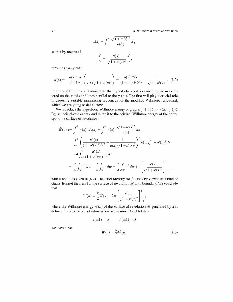
370 8 Willmore surfaces of revolution
s(x) =∫ x
−1
√1+u′(ξ )2
u(ξ )dξ
so that by means ofdds
=u(x)√
1+u′(x)2
ddx
,
formula (8.4) yields
κ(x) =−u(x)2
u′(x)ddx
(1
u(x)√
1+u′(x)2
)=
u(x)u′′(x)(1+u′(x)2)3/2 +
1√1+u′(x)2
. (8.5)
From these formulae it is immediate that hyperbolic geodesics are circular arcs cen-tered on the x-axis and lines parallel to the y-axis. The first will play a crucial rolein choosing suitable minimising sequences for the modified Willmore functional,which we are going to define now.
We introduce the hyperbolic Willmore energy of graphs [−1,1]3 x 7→ (x,u(x))∈R2
+ as their elastic energy and relate it to the original Willmore energy of the corre-sponding surface of revolution.
W (u) :=∫ 1
−1κ(x)2 ds(x) =
∫ 1
−1κ(x)2
√1+u′(x)2
u(x)dx
=∫ 1
−1
(u′′(x)
(1+u′(x)2)3/2 −1
u(x)√
1+u′(x)2
)2
u(x)√
1+u′(x)2 dx
+4∫ 1
−1
u′′(x)(1+u′(x)2)3/2 dx
=2π
∫RH2 dω− 2
π
∫RKdω =
2π
∫RH2 dω +4
[u′(x)√
1+u′(x)2
]1
−1
,
with H and K as given in (8.2). The latter identity for∫K may be viewed as a kind of
Gauss-Bonnet theorem for the surface of revolution R with boundary. We concludethat
W (u) =π
2W (u)−2π
[u′(x)√
1+u′(x)2
]1
−1
,
where the Willmore energy W (u) of the surface of revolution R generated by u isdefined in (8.3). In our situation where we assume Dirichlet data
u(±1) = α, u′(±1) = 0,
we even haveW (u) =
π
2W (u). (8.6)
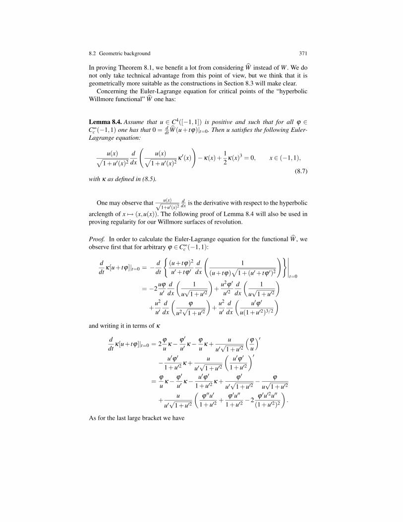
8.2 Geometric background 371
In proving Theorem 8.1, we benefit a lot from considering W instead of W . We donot only take technical advantage from this point of view, but we think that it isgeometrically more suitable as the constructions in Section 8.3 will make clear.
Concerning the Euler-Lagrange equation for critical points of the “hyperbolicWillmore functional” W one has:
Lemma 8.4. Assume that u ∈ C4([−1,1]) is positive and such that for all ϕ ∈C∞
c (−1,1) one has that 0 = ddt W (u + tϕ)|t=0. Then u satisfies the following Euler-
Lagrange equation:
u(x)√1+u′(x)2
ddx
(u(x)√
1+u′(x)2κ′(x)
)−κ(x)+
12
κ(x)3 = 0, x ∈ (−1,1),
(8.7)with κ as defined in (8.5).
One may observe that u(x)√1+u′(x)2
ddx is the derivative with respect to the hyperbolic
arclength of x 7→ (x,u(x)). The following proof of Lemma 8.4 will also be used inproving regularity for our Willmore surfaces of revolution.
Proof. In order to calculate the Euler-Lagrange equation for the functional W , weobserve first that for arbitrary ϕ ∈C∞
c (−1,1):
ddt
κ[u+ tϕ]|t=0 = − ddt
(u+ tϕ)2
u′+ tϕ ′ddx
(1
(u+ tϕ)√
1+(u′+ tϕ ′)2
)∣∣∣∣∣t=0
= −2uϕ
u′ddx
(1
u√
1+u′2
)+
u2ϕ ′
u′2ddx
(1
u√
1+u′2
)+
u2
u′ddx
(ϕ
u2√
1+u′2
)+
u2
u′ddx
(u′ϕ ′
u(1+u′2)3/2
)and writing it in terms of κ
ddt
κ[u+ tϕ]|t=0 = 2ϕ
uκ− ϕ ′
u′κ− ϕ
uκ +
u
u′√
1+u′2
(ϕ
u
)′− u′ϕ ′
1+u′2κ +
u
u′√
1+u′2
(u′ϕ ′
1+u′2
)′=
ϕ
uκ− ϕ ′
u′κ− u′ϕ ′
1+u′2κ +
ϕ ′
u′√
1+u′2− ϕ
u√
1+u′2
+u
u′√
1+u′2
(ϕ ′′u′
1+u′2+
ϕ ′u′′
1+u′2−2
ϕ ′u′2u′′
(1+u′2)2
).
As for the last large bracket we have
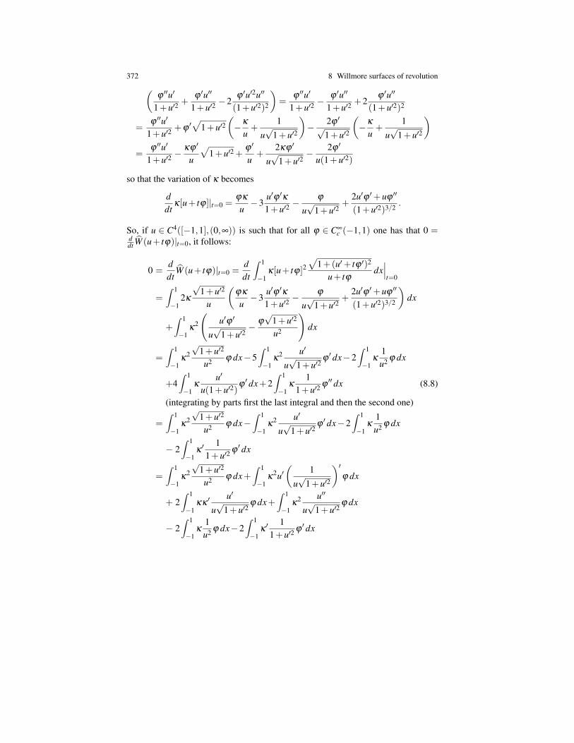
372 8 Willmore surfaces of revolution(ϕ ′′u′
1+u′2+
ϕ ′u′′
1+u′2−2
ϕ ′u′2u′′
(1+u′2)2
)=
ϕ ′′u′
1+u′2− ϕ ′u′′
1+u′2+2
ϕ ′u′′
(1+u′2)2
=ϕ ′′u′
1+u′2+ϕ
′√
1+u′2(−κ
u+
1u√
1+u′2
)− 2ϕ ′√
1+u′2
(−κ
u+
1u√
1+u′2
)=
ϕ ′′u′
1+u′2− κϕ ′
u
√1+u′2 +
ϕ ′
u+
2κϕ ′
u√
1+u′2− 2ϕ ′
u(1+u′2)
so that the variation of κ becomes
ddt
κ[u+ tϕ]|t=0 =ϕκ
u−3
u′ϕ ′κ1+u′2
− ϕ
u√
1+u′2+
2u′ϕ ′+uϕ ′′
(1+u′2)3/2 .
So, if u ∈ C4([−1,1],(0,∞)) is such that for all ϕ ∈ C∞c (−1,1) one has that 0 =
ddt W (u+ tϕ)|t=0, it follows:
0 =ddt
W (u+ tϕ)|t=0 =ddt
∫ 1
−1κ[u+ tϕ]2
√1+(u′+ tϕ ′)2
u+ tϕdx∣∣∣t=0
=∫ 1
−12κ
√1+u′2
u
(ϕκ
u−3
u′ϕ ′κ1+u′2
− ϕ
u√
1+u′2+
2u′ϕ ′+uϕ ′′
(1+u′2)3/2
)dx
+∫ 1
−1κ
2
(u′ϕ ′
u√
1+u′2− ϕ
√1+u′2
u2
)dx
=∫ 1
−1κ
2
√1+u′2
u2 ϕ dx−5∫ 1
−1κ
2 u′
u√
1+u′2ϕ′ dx−2
∫ 1
−1κ
1u2 ϕ dx
+4∫ 1
−1κ
u′
u(1+u′2)ϕ′ dx+2
∫ 1
−1κ
11+u′2
ϕ′′ dx (8.8)
(integrating by parts first the last integral and then the second one)
=∫ 1
−1κ
2
√1+u′2
u2 ϕ dx−∫ 1
−1κ
2 u′
u√
1+u′2ϕ′ dx−2
∫ 1
−1κ
1u2 ϕ dx
− 2∫ 1
−1κ′ 11+u′2
ϕ′ dx
=∫ 1
−1κ
2
√1+u′2
u2 ϕ dx+∫ 1
−1κ
2u′(
1u√
1+u′2
)′ϕ dx
+ 2∫ 1
−1κκ
′ u′
u√
1+u′2ϕ dx+
∫ 1
−1κ
2 u′′
u√
1+u′2ϕ dx
− 2∫ 1
−1κ
1u2 ϕ dx−2
∫ 1
−1κ′ 11+u′2
ϕ′ dx
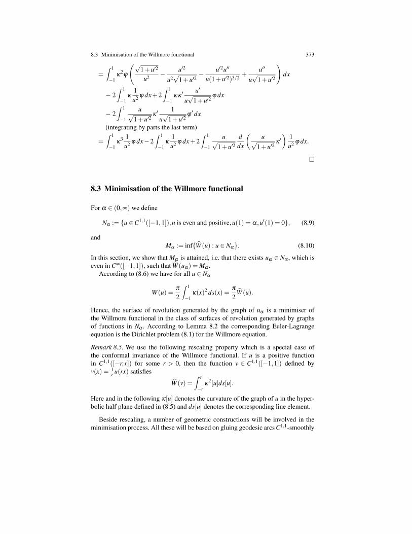
8.3 Minimisation of the Willmore functional 373
=∫ 1
−1κ
2ϕ
(√1+u′2
u2 − u′2
u2√
1+u′2− u′2u′′
u(1+u′2)3/2 +u′′
u√
1+u′2
)dx
− 2∫ 1
−1κ
1u2 ϕ dx+2
∫ 1
−1κκ
′ u′
u√
1+u′2ϕ dx
− 2∫ 1
−1
u√1+u′2
κ′ 1u√
1+u′2ϕ′ dx
(integrating by parts the last term)
=∫ 1
−1κ
3 1u2 ϕ dx−2
∫ 1
−1κ
1u2 ϕ dx+2
∫ 1
−1
u√1+u′2
ddx
(u√
1+u′2κ′)
1u2 ϕ dx.
8.3 Minimisation of the Willmore functional
For α ∈ (0,∞) we define
Nα := u ∈C1,1([−1,1]),u is even and positive,u(1) = α,u′(1) = 0, (8.9)
andMα := infW (u) : u ∈ Nα. (8.10)
In this section, we show that Mα is attained, i.e. that there exists uα ∈ Nα , which iseven in C∞([−1,1]), such that W (uα) = Mα .
According to (8.6) we have for all u ∈ Nα
W (u) =π
2
∫ 1
−1κ(x)2 ds(x) =
π
2W (u).
Hence, the surface of revolution generated by the graph of uα is a minimiser ofthe Willmore functional in the class of surfaces of revolution generated by graphsof functions in Nα . According to Lemma 8.2 the corresponding Euler-Lagrangeequation is the Dirichlet problem (8.1) for the Willmore equation.
Remark 8.5. We use the following rescaling property which is a special case ofthe conformal invariance of the Willmore functional. If u is a positive functionin C1,1([−r,r]) for some r > 0, then the function v ∈ C1,1([−1,1]) defined byv(x) = 1
r u(rx) satisfies
W (v) =∫ r
−rκ
2[u]ds[u].
Here and in the following κ[u] denotes the curvature of the graph of u in the hyper-bolic half plane defined in (8.5) and ds[u] denotes the corresponding line element.
Beside rescaling, a number of geometric constructions will be involved in theminimisation process. All these will be based on gluing geodesic arcs C1,1-smoothly

374 8 Willmore surfaces of revolution
to suitable parts of comparison functions for Mα or elements of minimising se-quences respectively. In a first step we will give an accurate bound from above forthe optimal Willmore energy Mα . The proof will be developed further in order toshow that α 7→ Mα is decreasing. Finally, by further refining these gluing tech-niques we come up with suitable minimising sequences obeying strong C1 a prioribounds and related qualitative properties. Basing on these properties a minimiser ofthe Willmore functional is obtained by using direct methods from the calculus ofvariation.
8.3.1 An upper bound for the optimal energy
Lemma 8.6. Let Mα be defined as in (8.10). Then
Mα ≤ 8tanh(
1α
).
In particular, limα→∞ Mα = 0.
Proof. For x 6= 0 let v(x) := α cosh((|x| − 1)/α). The corresponding surface ofrevolution consists of two branches of minimal surfaces with v(±1) = α , v′(±1) =0. Moreover, let x0 ∈ (0,1) be the uniquely determined point in (0,1) such that
0 = x0 + v(x0)v′(x0), and r =√
x20 + v(x0)2. One may observe that x0 + v(x0)v′(x0)
is the intersection point of the euclidean normal of the graph of v in (x0,v(x0)) withthe x-axis. We consider the C1,1 comparison function
u(x) :=
v(x) for x0 ≤ |x| ≤ 1,√
r2− x2 for 0≤ |x| ≤ x0.
See Figure 8.1.For the hyperbolic Willmore energy we compute
W (u) = 21∫
x0
(u′′
(1+u′2)32− 1
u√
1+u′2
)2
u√
1+u′2 dx+81∫
x0
u′′
(1+u′2)32
dx
= 81∫
x0
u′′
(1+u′2)32
dx =−8v′(x0)√
1+ v′(x0)2= 8tanh
(1− x0
α
)
≤ 8tanh(
1α
)< 8min1,1/α,
and the claim follows.
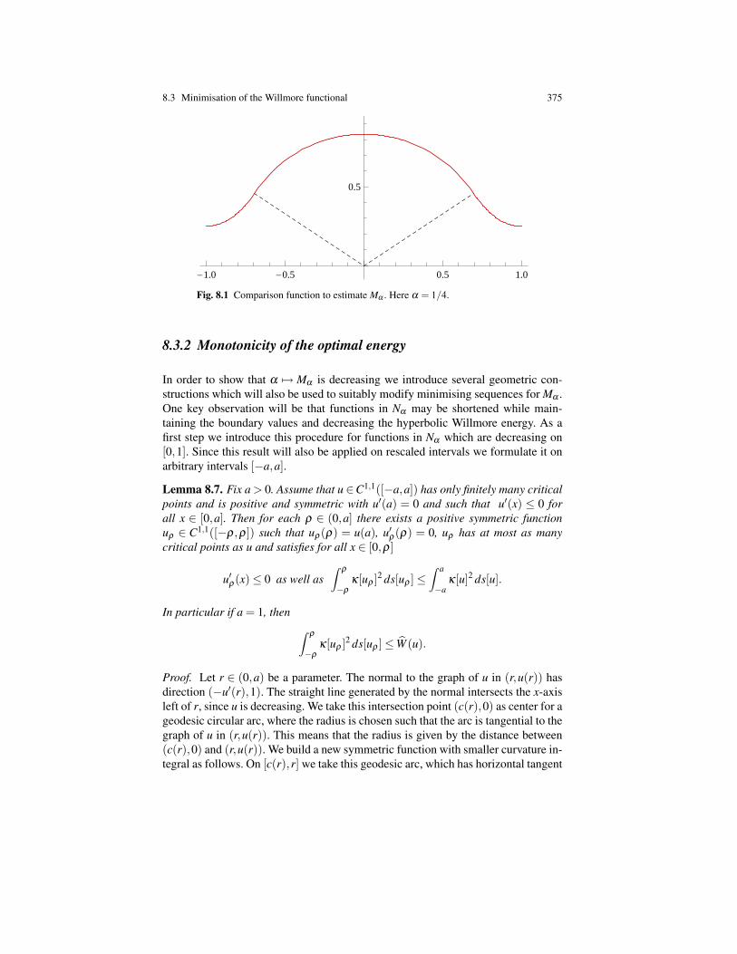
8.3 Minimisation of the Willmore functional 375
-1.0 -0.5 0.5 1.0
0.5
1.0
1.5
2.0
Fig. 8.1 Comparison function to estimate Mα . Here α = 1/4.
8.3.2 Monotonicity of the optimal energy
In order to show that α 7→ Mα is decreasing we introduce several geometric con-structions which will also be used to suitably modify minimising sequences for Mα .One key observation will be that functions in Nα may be shortened while main-taining the boundary values and decreasing the hyperbolic Willmore energy. As afirst step we introduce this procedure for functions in Nα which are decreasing on[0,1]. Since this result will also be applied on rescaled intervals we formulate it onarbitrary intervals [−a,a].
Lemma 8.7. Fix a > 0. Assume that u ∈C1,1([−a,a]) has only finitely many criticalpoints and is positive and symmetric with u′(a) = 0 and such that u′(x) ≤ 0 forall x ∈ [0,a]. Then for each ρ ∈ (0,a] there exists a positive symmetric functionuρ ∈ C1,1([−ρ,ρ]) such that uρ(ρ) = u(a), u′ρ(ρ) = 0, uρ has at most as manycritical points as u and satisfies for all x ∈ [0,ρ]
u′ρ(x)≤ 0 as well as∫
ρ
−ρ
κ[uρ ]2 ds[uρ ]≤∫ a
−aκ[u]2 ds[u].
In particular if a = 1, then ∫ρ
−ρ
κ[uρ ]2 ds[uρ ]≤ W (u).
Proof. Let r ∈ (0,a) be a parameter. The normal to the graph of u in (r,u(r)) hasdirection (−u′(r),1). The straight line generated by the normal intersects the x-axisleft of r, since u is decreasing. We take this intersection point (c(r),0) as center for ageodesic circular arc, where the radius is chosen such that the arc is tangential to thegraph of u in (r,u(r)). This means that the radius is given by the distance between(c(r),0) and (r,u(r)). We build a new symmetric function with smaller curvature in-tegral as follows. On [c(r),r] we take this geodesic arc, which has horizontal tangent
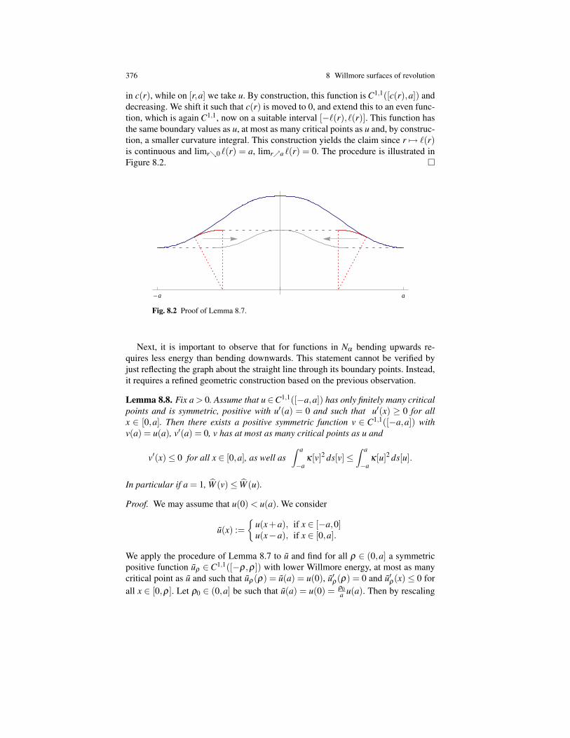
376 8 Willmore surfaces of revolution
in c(r), while on [r,a] we take u. By construction, this function is C1,1([c(r),a]) anddecreasing. We shift it such that c(r) is moved to 0, and extend this to an even func-tion, which is again C1,1, now on a suitable interval [−`(r), `(r)]. This function hasthe same boundary values as u, at most as many critical points as u and, by construc-tion, a smaller curvature integral. This construction yields the claim since r 7→ `(r)is continuous and limr0 `(r) = a, limra `(r) = 0. The procedure is illustrated inFigure 8.2.
-a a
Fig. 8.2 Proof of Lemma 8.7.
Next, it is important to observe that for functions in Nα bending upwards re-quires less energy than bending downwards. This statement cannot be verified byjust reflecting the graph about the straight line through its boundary points. Instead,it requires a refined geometric construction based on the previous observation.
Lemma 8.8. Fix a > 0. Assume that u ∈C1,1([−a,a]) has only finitely many criticalpoints and is symmetric, positive with u′(a) = 0 and such that u′(x) ≥ 0 for allx ∈ [0,a]. Then there exists a positive symmetric function v ∈ C1,1([−a,a]) withv(a) = u(a), v′(a) = 0, v has at most as many critical points as u and
v′(x)≤ 0 for all x ∈ [0,a], as well as∫ a
−aκ[v]2 ds[v]≤
∫ a
−aκ[u]2 ds[u].
In particular if a = 1, W (v)≤ W (u).
Proof. We may assume that u(0) < u(a). We consider
u(x) :=
u(x+a), if x ∈ [−a,0]u(x−a), if x ∈ [0,a].
We apply the procedure of Lemma 8.7 to u and find for all ρ ∈ (0,a] a symmetricpositive function uρ ∈C1,1([−ρ,ρ]) with lower Willmore energy, at most as manycritical point as u and such that uρ(ρ) = u(a) = u(0), u′ρ(ρ) = 0 and u′ρ(x)≤ 0 forall x ∈ [0,ρ]. Let ρ0 ∈ (0,a] be such that u(a) = u(0) = ρ0
a u(a). Then by rescaling
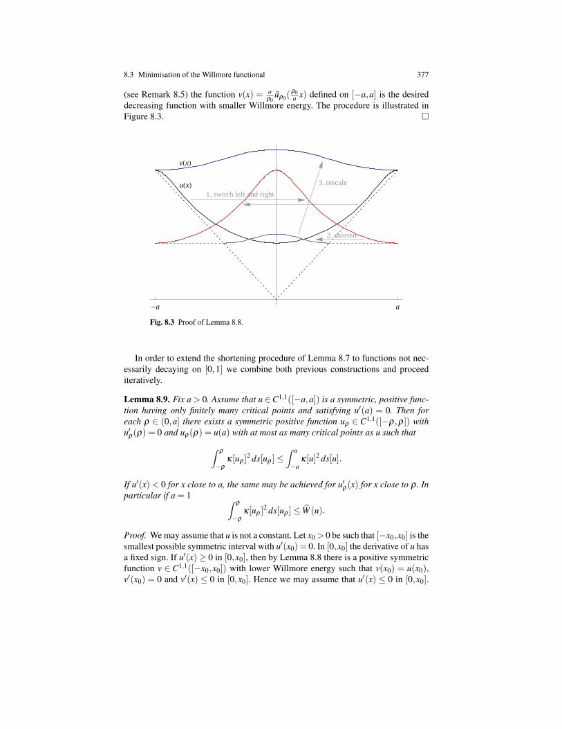
8.3 Minimisation of the Willmore functional 377
(see Remark 8.5) the function v(x) = aρ0
uρ0(ρ0a x) defined on [−a,a] is the desired
decreasing function with smaller Willmore energy. The procedure is illustrated inFigure 8.3.
uHxL
vHxL
1. switch left and right
2. shorten
3. rescale
-a a
Fig. 8.3 Proof of Lemma 8.8.
In order to extend the shortening procedure of Lemma 8.7 to functions not nec-essarily decaying on [0,1] we combine both previous constructions and proceediteratively.
Lemma 8.9. Fix a > 0. Assume that u ∈C1,1([−a,a]) is a symmetric, positive func-tion having only finitely many critical points and satisfying u′(a) = 0. Then foreach ρ ∈ (0,a] there exists a symmetric positive function uρ ∈ C1,1([−ρ,ρ]) withu′ρ(ρ) = 0 and uρ(ρ) = u(a) with at most as many critical points as u such that∫
ρ
−ρ
κ[uρ ]2 ds[uρ ]≤∫ a
−aκ[u]2 ds[u].
If u′(x) < 0 for x close to a, the same may be achieved for u′ρ(x) for x close to ρ . Inparticular if a = 1 ∫
ρ
−ρ
κ[uρ ]2 ds[uρ ]≤ W (u).
Proof. We may assume that u is not a constant. Let x0 > 0 be such that [−x0,x0] is thesmallest possible symmetric interval with u′(x0) = 0. In [0,x0] the derivative of u hasa fixed sign. If u′(x)≥ 0 in [0,x0], then by Lemma 8.8 there is a positive symmetricfunction v ∈ C1,1([−x0,x0]) with lower Willmore energy such that v(x0) = u(x0),v′(x0) = 0 and v′(x) ≤ 0 in [0,x0]. Hence we may assume that u′(x) ≤ 0 in [0,x0].
378 8 Willmore surfaces of revolution
By Lemma 8.7 for all r ∈ (0,x0] there exists a positive symmetric function vr ∈C1,1([−r,r]) such that vr(r) = u(x0) and v′r(r) = 0 and v′r(x)≤ 0 in [0,r]. Hence thefunction
ur(x) :=
u(x+ x0− r), if r < x≤ a+ r− x0,vr(x), if − r ≤ x≤ r,u(x− x0 + r), if −a− r + x0 < x≤−r,
is in C1,1([−a−r+x0,a+r−x0]), is symmetric, u′r(a+r−x0) = 0, ur(a+r−x0) =u(a) and ∫ a+r−x0
−(a+r−x0)κ[ur]2 ds[ur]≤
∫ a
−aκ[u]2 ds[u].
With this construction the claim is proved for ρ ≥ a− x0.For ρ < a− x0 we start from the function just constructed obtained at the limit
for r going to zero. That is v(x) = u(x + x0) for x ∈ [0,a− x0] and extended bysymmetry on [−a + x0,0]. This function is in C1,1([−a + x0,a− x0]), positive andsymmetric. We can repeat the same construction just done. We continuously de-crease the interval of definition and, at the same time, the curvature integral. Sincewe have only finitely many critical points and at each iteration step we decrease thenumber of critical points, this procedure is well-defined and terminates after finitelymany iterations.
If u′ < 0 close to a the same may be achieved for u′ρ since in the construction wedo not change the function near the end-points of the interval of definition.
Corollary 8.10. Fix a > 0 and α > 0. For each positive symmetric u∈C1,1([−a,a])having only finitely many critical points and satisfying
u(±a) = α, u′(±a) = 0
and for each β ≥ α , there exists a symmetric positive function v ∈ C1,1([−a,a])having at most as many critical points as u, satisfying
v(±a) = β , v′(±a) = 0
and ∫ a
−aκ[v]2 ds[v]≤
∫ a
−aκ[u]2 ds[u].
If u′(x) < 0 for x close to a, the same may be achieved for v′. In particular, if a = 1then W (v)≤ W (u).
Proof. By Lemma 8.9 for each ρ ∈ (0,a], there exists a symmetric positive functionuρ ∈C1,1([−ρ,ρ]) having at most as many critical points as u with u′ρ(ρ) = 0 anduρ(ρ) = u(a) = α such that∫
ρ
−ρ
κ[uρ ]2 ds[uρ ]≤∫ a
−aκ[u]2 ds[u].
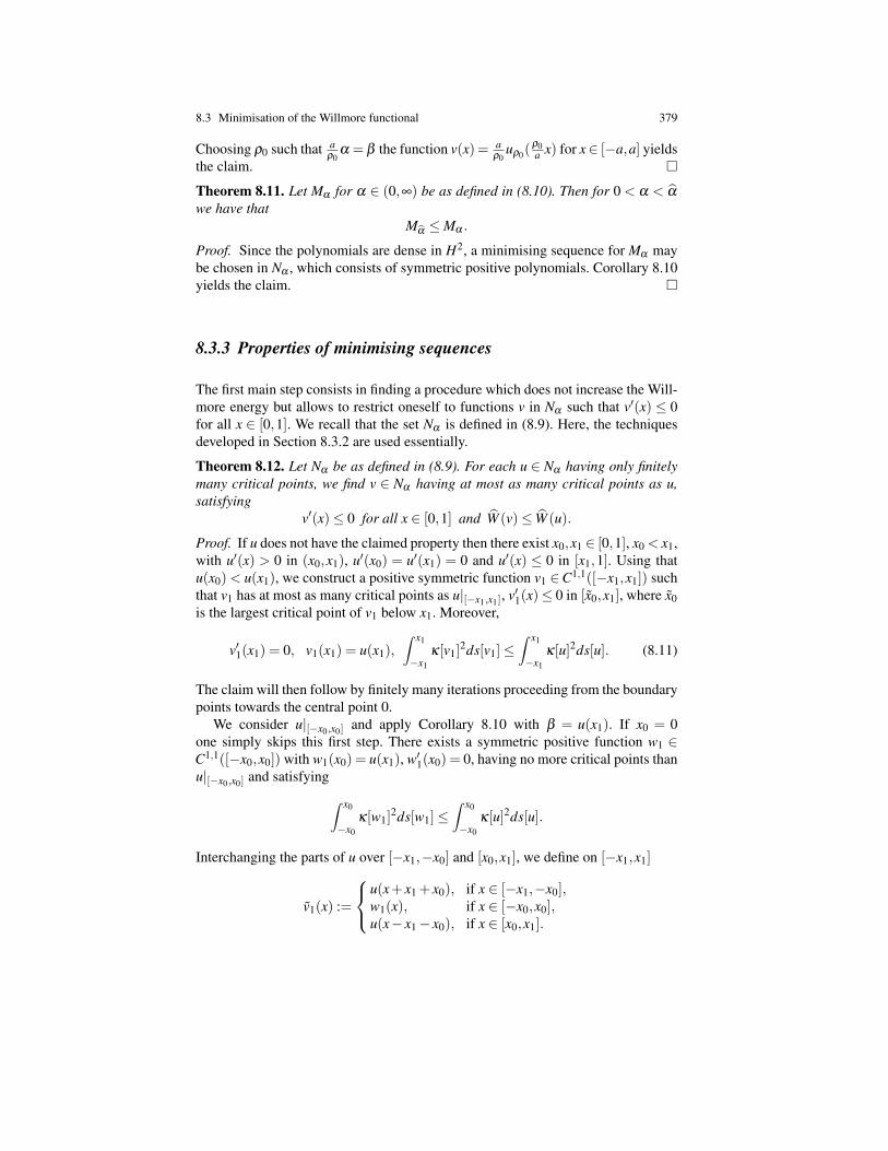
8.3 Minimisation of the Willmore functional 379
Choosing ρ0 such that aρ0
α = β the function v(x) = aρ0
uρ0(ρ0a x) for x∈ [−a,a] yields
the claim.
Theorem 8.11. Let Mα for α ∈ (0,∞) be as defined in (8.10). Then for 0 < α < α
we have thatMα ≤Mα .
Proof. Since the polynomials are dense in H2, a minimising sequence for Mα maybe chosen in Nα , which consists of symmetric positive polynomials. Corollary 8.10yields the claim.
8.3.3 Properties of minimising sequences
The first main step consists in finding a procedure which does not increase the Will-more energy but allows to restrict oneself to functions v in Nα such that v′(x) ≤ 0for all x ∈ [0,1]. We recall that the set Nα is defined in (8.9). Here, the techniquesdeveloped in Section 8.3.2 are used essentially.
Theorem 8.12. Let Nα be as defined in (8.9). For each u ∈ Nα having only finitelymany critical points, we find v ∈ Nα having at most as many critical points as u,satisfying
v′(x)≤ 0 for all x ∈ [0,1] and W (v)≤ W (u).
Proof. If u does not have the claimed property then there exist x0,x1 ∈ [0,1], x0 < x1,with u′(x) > 0 in (x0,x1), u′(x0) = u′(x1) = 0 and u′(x) ≤ 0 in [x1,1]. Using thatu(x0) < u(x1), we construct a positive symmetric function v1 ∈C1,1([−x1,x1]) suchthat v1 has at most as many critical points as u|[−x1,x1], v′1(x)≤ 0 in [x0,x1], where x0is the largest critical point of v1 below x1. Moreover,
v′1(x1) = 0, v1(x1) = u(x1),∫ x1
−x1
κ[v1]2ds[v1]≤∫ x1
−x1
κ[u]2ds[u]. (8.11)
The claim will then follow by finitely many iterations proceeding from the boundarypoints towards the central point 0.
We consider u|[−x0,x0] and apply Corollary 8.10 with β = u(x1). If x0 = 0one simply skips this first step. There exists a symmetric positive function w1 ∈C1,1([−x0,x0]) with w1(x0) = u(x1), w′1(x0) = 0, having no more critical points thanu|[−x0,x0] and satisfying∫ x0
−x0
κ[w1]2ds[w1]≤∫ x0
−x0
κ[u]2ds[u].
Interchanging the parts of u over [−x1,−x0] and [x0,x1], we define on [−x1,x1]
v1(x) :=
u(x+ x1 + x0), if x ∈ [−x1,−x0],w1(x), if x ∈ [−x0,x0],u(x− x1− x0), if x ∈ [x0,x1].
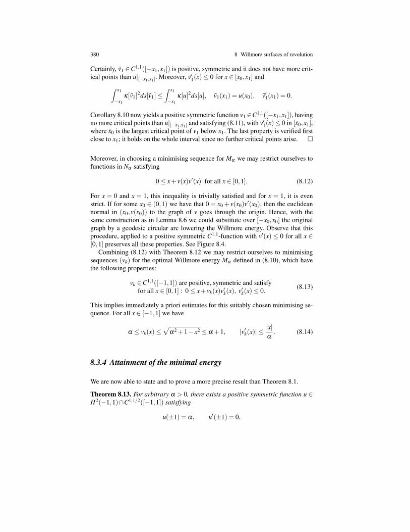
380 8 Willmore surfaces of revolution
Certainly, v1 ∈C1,1([−x1,x1]) is positive, symmetric and it does not have more crit-ical points than u|[−x1,x1]. Moreover, v′1(x)≤ 0 for x ∈ [x0,x1] and∫ x1
−x1
κ[v1]2ds[v1]≤∫ x1
−x1
κ[u]2ds[u], v1(x1) = u(x0), v′1(x1) = 0.
Corollary 8.10 now yields a positive symmetric function v1 ∈C1,1([−x1,x1]), havingno more critical points than u|[−x1,x1] and satisfying (8.11), with v′1(x)≤ 0 in [x0,x1],where x0 is the largest critical point of v1 below x1. The last property is verified firstclose to x1; it holds on the whole interval since no further critical points arise.
Moreover, in choosing a minimising sequence for Mα we may restrict ourselves tofunctions in Nα satisfying
0≤ x+ v(x)v′(x) for all x ∈ [0,1]. (8.12)
For x = 0 and x = 1, this inequality is trivially satisfied and for x = 1, it is evenstrict. If for some x0 ∈ (0,1) we have that 0 = x0 + v(x0)v′(x0), then the euclideannormal in (x0,v(x0)) to the graph of v goes through the origin. Hence, with thesame construction as in Lemma 8.6 we could substitute over [−x0,x0] the originalgraph by a geodesic circular arc lowering the Willmore energy. Observe that thisprocedure, applied to a positive symmetric C1,1-function with v′(x) ≤ 0 for all x ∈[0,1] preserves all these properties. See Figure 8.4.
Combining (8.12) with Theorem 8.12 we may restrict ourselves to minimisingsequences (vk) for the optimal Willmore energy Mα defined in (8.10), which havethe following properties:
vk ∈C1,1([−1,1]) are positive, symmetric and satisfyfor all x ∈ [0,1] : 0≤ x+ vk(x)v′k(x), v′k(x)≤ 0.
(8.13)
This implies immediately a priori estimates for this suitably chosen minimising se-quence. For all x ∈ [−1,1] we have
α ≤ vk(x)≤√
α2 +1− x2 ≤ α +1, |v′k(x)| ≤|x|α
. (8.14)
8.3.4 Attainment of the minimal energy
We are now able to state and to prove a more precise result than Theorem 8.1.
Theorem 8.13. For arbitrary α > 0, there exists a positive symmetric function u ∈H2(−1,1)∩C1,1/2([−1,1]) satisfying
u(±1) = α, u′(±1) = 0,
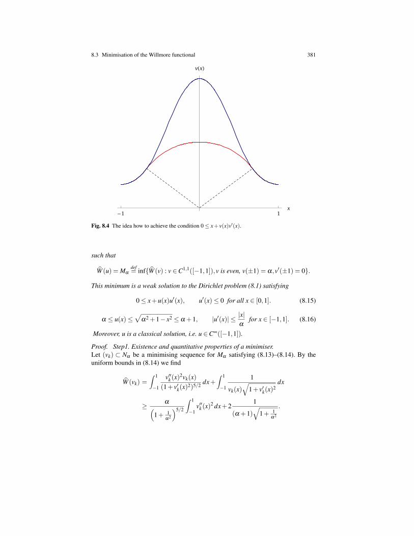
8.3 Minimisation of the Willmore functional 381
-1 1x
vHxL
Fig. 8.4 The idea how to achieve the condition 0≤ x+ v(x)v′(x).
such that
W (u) = Mα
def= infW (v) : v ∈C1,1([−1,1]),v is even, v(±1) = α,v′(±1) = 0.
This minimum is a weak solution to the Dirichlet problem (8.1) satisfying
0≤ x+u(x)u′(x), u′(x)≤ 0 for all x ∈ [0,1]. (8.15)
α ≤ u(x)≤√
α2 +1− x2 ≤ α +1, |u′(x)| ≤ |x|α
for x ∈ [−1,1]. (8.16)
Moreover, u is a classical solution, i.e. u ∈C∞([−1,1]).
Proof. Step1. Existence and quantitative properties of a minimiser.Let (vk) ⊂ Nα be a minimising sequence for Mα satisfying (8.13)–(8.14). By theuniform bounds in (8.14) we find
W (vk) =∫ 1
−1
v′′k (x)2vk(x)
(1+ v′k(x)2)5/2 dx+
∫ 1
−1
1
vk(x)√
1+ v′k(x)2
dx
≥ α(1+ 1
α2
)5/2
∫ 1
−1v′′k (x)
2 dx+21
(α +1)√
1+ 1α2
.
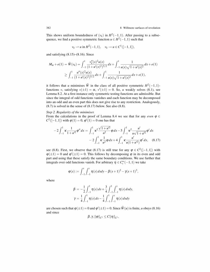
382 8 Willmore surfaces of revolution
This shows uniform boundedness of (vk) in H2(−1,1). After passing to a subse-quence, we find a positive symmetric function u ∈ H2(−1,1) such that
vk u in H2(−1,1), vk → u ∈C1([−1,1]),
and satisfying (8.15)–(8.16). Since
Mα +o(1) = W (vk) =∫ 1
−1
v′′k (x)2u(x)
(1+u′(x)2)5/2 dx+∫ 1
−1
1
u(x)√
1+u′(x)2dx+o(1)
≥∫ 1
−1
u′′(x)2u(x)(1+u′(x)2)5/2 dx+
∫ 1
−1
1
u(x)√
1+u′(x)2dx+o(1),
it follows that u minimises W in the class of all positive symmetric H2(−1,1)-functions v, satisfying v(±1) = α , v′(±1) = 0. So, u weakly solves (8.1), seeLemma 8.2. At a first instance only symmetric testing functions are admissible. Butsince the integral of odd functions vanishes and each function may be decomposedinto an odd and an even part this does not give rise to any restriction. Analogously,(8.7) is solved in the sense of (8.17) below. See also (8.8).
Step 2. Regularity of the minimiser.From the calculations in the proof of Lemma 8.4 we see that for any even ϕ ∈C2([−1,1]) with ϕ(1) = 0, ϕ ′(1) = 0 one has that
−2∫ 1
−1κ
11+u′2
ϕ′′ dx =
∫ 1
−1κ
2
√1+u′2
u2 ϕ dx−5∫ 1
−1κ
2 u′
u√
1+u′2ϕ′ dx
− 2∫ 1
−1κ
1u2 ϕ dx+4
∫ 1
−1κ
u′
u(1+u′2)ϕ′ dx, (8.17)
see (8.8). First, we observe that (8.17) is still true for any ϕ ∈ C2([−1,1]) withϕ(±1) = 0 and ϕ ′(±1) = 0. This follows by decomposing ϕ in its even and oddpart and using that these satisfy the same boundary conditions. We use further thatintegrals over odd functions vanish. For arbitrary η ∈C∞
c (−1,1) we take
ϕ(x) :=∫ x
−1
∫ y
−1η(s)dsdy−β (x+1)2− γ(x+1)3,
where
β = −12
∫ 1
−1η(s)ds+
34
∫ 1
−1
∫ y
−1η(s)dsdy,
γ =14
∫ 1
−1η(s)ds− 1
4
∫ 1
−1
∫ y
−1η(s)dsdy
are chosen such that ϕ(±1) = 0 and ϕ ′(±1) = 0. Since W (u) is finite, u obeys (8.16)and since
β ,γ,‖ϕ‖C1 ≤C‖η‖L1 ,
8.4 Bibliographical notes 383
we can conclude from (8.17) that for each η ∈C∞c (−1,1),∣∣∣∣∫ 1
−1κ
11+u′2
η dx∣∣∣∣≤C(u)‖η‖L1 .
By the bounds on u in (8.16), the above inequality shows that κ is bounded and so,
u ∈W 2,∞(−1,1).
Next, for arbitrary η ∈C∞c (−1,1) we choose
ϕ(x) =∫ x
−1η(s)ds− 3
4
(∫ 1
−1η(s)ds
)(x+1)2 +
14
(∫ 1
−1η(s)ds
)(x+1)3
so that
ϕ(±1) = 0, ϕ′(±1) = 0, ‖ϕ‖C0 ≤C‖η‖L1 , ‖ϕ
′‖L1 ≤C‖η‖L1 .
Since we already know that κ is bounded, we conclude from (8.17) that for eachη ∈C∞
c (−1,1), ∣∣∣∣∫ 1
−1κ
11+u′2
η′(x)dx
∣∣∣∣≤C(u)‖η‖L1 .
This proves that
κ1
1+u′2∈W 1,∞(−1,1), κ ∈W 1,∞([−1,1]) = C0,1([−1,1]),
u ∈W 3,∞([−1,1]) = C2,1([−1,1]).
Finally, rewriting (8.7) as follows
ddx
(u(x)√
1+u′(x)2κ′(x)
)=
√1+u′(x)2
u(x)(κ(x)− 1
2κ(x)3) in (−1,1),
we get an equation for κ with W 1,∞-coefficients and right hand side. Hence,κ ∈W 3,∞([−1,1]) = C2,1([−1,1]), u ∈C4,1([−1,1]) and finally, by straightforwardbootstrapping, u ∈C∞([−1,1]).
8.4 Bibliographical notes
A historical survey over the Willmore functional and a profound discussion of mod-eling aspects is provided by Nitsche [324]. There, also Euler-Lagrange equationsare deduced and sets of natural boundary conditions are discussed. The Willmorefunctional was already considered as a model for the elastic energy of thin plates inthe 19th century, see e.g. [341], but a mathematical treatment seemed to have been
384 8 Willmore surfaces of revolution
out of reach for more than 100 years. It was popularised again in the second half ofthe 20th century by Willmore’s work, see e.g. [413, 414].
Existence of closed Willmore surfaces of prescribed genus was proved by Simonand Bauer-Kuwert [35, 371]. Riviere [355] showed a far reaching regularity result.Also, local and global existence results for the Willmore flow of closed surfacesare available, see e.g. [262, 263, 264, 372]. On the other hand, Mayer and Simonett[287] gave a numerical example providing evidence that for particular initial datathe Willmore flow may develop geometric singularities – change of topology – infinite time. An analytic proof for occurrence of such a singularity in finite or infi-nite time for the same initial data was given by Blatt [60]. The Willmore flow forone-dimensional closed curves was studied by Dziuk-Kuwert-Schatzle [156] andPolden [342].
Numerical experiments concerning Willmore surfaces of revolutions were per-formed by Frohlich [175], where as boundary data, the position α > 0 and the meancurvature H = 0 were prescribed. Bryant, Griffiths [77, 78] and Hertrich-Jeromin,Pinkall (see e.g. [229]) observed that Willmore surfaces of revolution can be consid-ered as elastic curves in the hyperbolic half space. This observation was exploitedin [266, 267], where also many properties of elastic curves in the hyperbolic halfspace were deduced. This reformulation helped a lot in proving our main result from[115], which is a joint work of Deckelnick, Dall’Acqua, and Grunau. The underly-ing geometric constructions benefit from previous works on related one-dimensionalproblems [137, 139]. More general Dirichlet prolems for Willmore surfaces of rev-olution are studied in [116], while Navier-type boundary value problems are subjectof [50, 138].
Quite recently, Schatzle [360] proved an important general result concerning ex-istence of branched Willmore immersions in Sn satisfying Dirichlet boundary con-ditions. Assuming the boundary data to obey some explicit geometrically motivatedsmallness condition these immersions can even be shown to be embedded. By work-ing in Sn, some compactness problems could be overcome. On the other hand, whenpulling pack these immersions to Rn it cannot be excluded that they contain ∞.Moreover, in general, the existence of branch points cannot be ruled out, and due tothe generality of the approach, it seems to us that only little topological informationabout the solutions can be extracted from the existence proof.
Notations, citations, and indexes
Notations
C positive constants in estimates, which may change theirvalue from term to term.
t+ maxt,0 for t ∈ R.
t− max−t,0 for t ∈ R.
ak ∼ bk limk→∞
ak
bk= 1.
N = 0,1,2,3 . . ..
N+ = 1,2,3 . . ..
n space dimension.
Rn+ = x ∈ Rn : x1 > 0, half space.
Ω domain, an open and connected subset of Rn.
∂Ω Ω ∩Rn \Ω , the boundary of Ω .
Ω0 ⊂⊂Ω Ω0 is compact and Ω0 ⊂Ω .
Ac for A⊂Ω : complement of A in Ω , Ω \A.
dω surface element for ∂Ω .
ν exterior unit normal at ∂Ω .
Br(x) open ball with radius r and centre x.
B = B1(0), open unit ball in Rn.
Sn−1 = ∂B⊂ Rn, unit sphere.
385
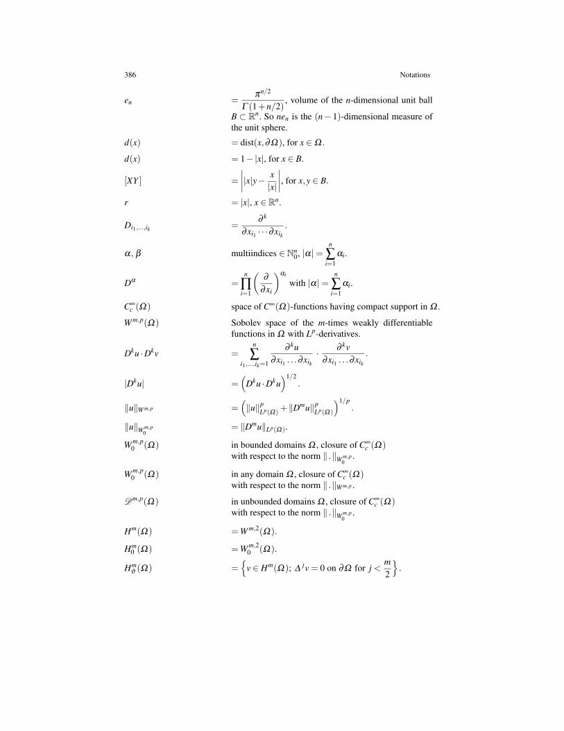
386 Notations
en =πn/2
Γ (1+n/2), volume of the n-dimensional unit ball
B ⊂ Rn. So nen is the (n− 1)-dimensional measure ofthe unit sphere.
d(x) = dist(x,∂Ω), for x ∈Ω .
d(x) = 1−|x|, for x ∈ B.
[XY ] =∣∣∣∣|x|y− x
|x|
∣∣∣∣, for x,y ∈ B.
r = |x|, x ∈ Rn.
Di1,...,ik =∂ k
∂xi1 · · ·∂xik.
α, β multiindices ∈ Nn0, |α|=
n
∑i=1
αi.
Dα =n
∏i=1
(∂
∂xi
)αi
with |α|=n
∑i=1
αi.
C∞c (Ω) space of C∞(Ω)-functions having compact support in Ω .
W m,p(Ω) Sobolev space of the m-times weakly differentiablefunctions in Ω with Lp-derivatives.
Dku ·Dkv =n
∑i1,...,ik=1
∂ ku∂xi1 . . .∂xik
· ∂ kv∂xi1 . . .∂xik
.
|Dku| =(
Dku ·Dku)1/2
.
‖u‖W m,p =(‖u‖p
Lp(Ω) +‖Dmu‖pLp(Ω)
)1/p.
‖u‖W m,p0
= ‖Dmu‖Lp(Ω).
W m,p0 (Ω) in bounded domains Ω , closure of C∞
c (Ω)with respect to the norm ‖ .‖W m,p
0.
W m,p0 (Ω) in any domain Ω , closure of C∞
c (Ω)with respect to the norm ‖ .‖W m,p .
Dm,p(Ω) in unbounded domains Ω , closure of C∞c (Ω)
with respect to the norm ‖ .‖W m,p0
.
Hm(Ω) = W m,2(Ω).
Hm0 (Ω) = W m,2
0 (Ω).
Hmϑ (Ω) =
v ∈ Hm(Ω); ∆
jv = 0 on ∂Ω for j <m2
.
Notations 387
H−m(Ω) dual space (Hm0 (Ω))′.
‖u‖2Hm
0=
n
∑i1,...,im=1
∫Ω
|Di1,...,im u|2 dx = (see (2.12))
=
∫
Ω
(∆
m/2u)2
dx if m is even,∫Ω
∣∣∣∇∆(m−1)/2u
∣∣∣2 dx if m is odd.
( . , .)Hm0
corresponding scalar product in Hm0 (Ω).
‖u‖2Dm,2 =
∫
Ω
(∆
m/2u)2
dx if m is even,∫Ω
∣∣∣∇∆(m−1)/2u
∣∣∣2 dx if m is odd.
( . , .)Dm,2 corresponding scalar product in Dm,2.
〈 f ,u〉 dual pairing: u ∈ Banach space, f ∈ its dual.
Λm, j j-th Dirichlet-eigenvalue of (−∆)m,according to its multiplicity.
ϕ j corresponding eigenfunctions, orthonormal in Hm0 (Ω).
Gm,n, Gm,n Green’s function, Green’s operator, resp. for (−∆)m
under Dirichlet boundary conditions in B⊂ Rn.
G(−∆)m,Ω , G(−∆)m,Ω the same for Ω ⊂ Rn.
Gm,n,A , Gm,n,A the same for (−∆)m +A in B⊂ Rn,where A u = ∑
|α|≤2m−1aα Dα u.
G(−∆)m,Ω ,A , G(−∆)m,Ω ,A the same in Ω ⊂ Rn.
s =n+2mn−2m
, for n > 2m; critical Sobolev exponent.
For measurable functions f :
f > 0 f (x) > 0 for almost all x.
f > g f −g > 0.
f 0 f (x) < 0 for x in a set of positive measure.
f g f −g 0.
f 0 f (x) 6= 0 for x in a set of positive measure and f (x)≥ 0for almost all x.
f g f −g 0.
f (t)' g(t) ∃C > 0 ∀ t :1C
f (t)≤ g(t)≤C f (t); for f ,g≥ 0.
388 Notations
f (t) g(t) ∃C > 0 ∀t : f (t)≤C g(t), for f ,g≥ 0.
Ω∗ a ball centered at the origin such that |Ω |= |Ω ∗|.
u∗ spherical rearrangement of a measurable function u, seeDefinition 3.10.
(gi j)i, j=1,...,n Riemannian metric, positive definite tensor. In case ofparametrisations X in R3 over a two dimensional pa-rameter domain: gi j = ∂iX ·∂ jX .
g = det((gi j)i, j=1,...,n
), Gram’s determinant.
(gi j)i, j=1,...,n inverse of the metric tensor.
(Li j)i, j=1,...,n second fundamental form. In case of parametrisationsX in R3 over a two dimensional parameter domain:
Li j =1√
gdet(∂i∂ jX ,∂1X ,∂2X) .
H mean curvature. In case of parametrisations X in R3
over a two dimensional parameter domain:
H=12
2
∑i, j=1
gi jLi j =1
2g(g22L11−2g12L12 +g11L22) .
K Gaussian curvature. In case of parametrisations X in R3
over a two dimensional parameter domain:
K=det((Li j)i, j=1,2
)g
.
.
Γ ki j =
n
∑`=1
12
gk` (∂ jgi` +∂ig j`−∂`gi j
), Christoffel symbols.
R`ki j =−R`
k ji = ∂iΓ`jk−∂ jΓ
`ik +
n
∑m=1
(Γ
`imΓ
mjk −Γ
`jmΓ
mik
),
Riemannian curvature tensor.
Rk`i j =−R`ki j = Ri jk` =n
∑m=1
gkmRm`i j.
Ri j =n
∑k,`=1
gk`Rik j` =n
∑k=1
Rkik j, Ricci tensor.
R =n
∑i, j=1
gi jRi j, scalar curvature.
Si j =1
n−2
(2Ri j−
R(n−1)
gi j
), Schouten tensor.
Notations 389
Wi jk` = Ri jk`−1
n−2(Rikg j`−Ri`g jk +R j`gik−R jkgi`
)+
R(n−1)(n−2)
(g j`gik−g jkgi`
), Weyl tensor.
390 Bibliography
Bibliography
1. R.A. Adams. Sobolev Spaces, volume 65 of Pure and Applied Mathematics. Academic Press,New York, London, 1975.
2. V. Adolfsson. L2-integrability of second-order derivatives for Poisson’s equation in nons-mooth domains. Math. Scand., 70:146–160, 1992.
3. S. Agmon. The coerciveness problem for integro-differential forms. J. Analyse Math., 6:183–223, 1958.
4. S. Agmon. Maximum theorems for solutions of higher order elliptic equations. Bull. Amer.Math. Soc., 66:77–80, 1960.
5. S. Agmon, A. Douglis, and L. Nirenberg. Estimates near the boundary for solutions of ellipticpartial differential equations satisfying general boundary conditions. I. Comm. Pure Appl.Math., 12:623–727, 1959.
6. S. Agmon, A. Douglis, and L. Nirenberg. Estimates near the boundary for solutions of ellipticpartial differential equations satisfying general boundary conditions. II. Comm. Pure Appl.Math., 17:35–92, 1964.
7. A.D. Alexandrov. A characteristic property of the spheres. Ann. Mat. Pura Appl., (4) 58:303–354, 1962.
8. E. Almansi. Sull’integrazione dell’equazione differenziale ∆ 2∆ 2 = 0. Rom. Acc. L. Rend.,(5) 81:104–107, 1899.
9. E. Almansi. Sull’integrazione dell’equazione differenziale ∆ 2n = 0. Annali di Mat., (3)2:1–51, 1899.
10. F.J. Almgren and E.H. Lieb. Symmetric decreasing rearrangement is sometimes continuous.J. Amer. Math. Soc., 2:683–773, 1989.
11. H.W. Alt. Lineare Funktionalanalysis, eine anwendungsorientierte Einfuhrung. 4.,uberarbeitete und erweiterte Aufl. Springer-Verlag, Berlin etc., 2002.
12. C.O. Alves and J.M. do O. Positive solutions of a fourth-order semilinear problem involvingcritical growth. Adv. Nonlinear Stud., 2:437–458, 2002.
13. H. Amann. Fixed point equations and nonlinear eigenvalue problems in ordered Banachspaces. SIAM Rev., 18:620–709, 1976. (Erratum in: SIAM Rev. 19: vii, 1977.).
14. A. Ambrosetti and P.H. Rabinowitz. Dual variational methods in critical point theory andapplications. J. Funct. Anal., 14:349–381, 1973.
15. A. Ambrosetti and M. Struwe. A note on the problem−∆u = λu+u|u|2∗−2. Manuscr. Math.,54:373–379, 1986.
16. O.H. Ammann, Th. von Karman, and G.B. Woodruff. The failure of the Tacoma NarrowsBridge. Federal Works Agency, 1941.
17. G.E. Andrews, R. Askey, and R. Roy. Special Functions, volume 71 of Encyclopedia ofMathematics and its applications. Cambridge University Press, Cambridge, 1999.
18. G. Arioli, F. Gazzola, and H.-Ch. Grunau. Entire solutions for a semilinear fourth orderelliptic problem with exponential nonlinearity. J. Differential Equations, 230:743–770, 2006.
19. G. Arioli, F. Gazzola, H.-Ch. Grunau, and E. Mitidieri. A semilinear fourth order ellipticproblem with exponential nonlinearity. SIAM J. Math. Anal., 36:1226–1258, 2005.
20. G. Arioli, F. Gazzola, H.-Ch. Grunau, and E. Sassone. The second bifurcation branch forradial solutions of the Brezis-Nirenberg problem in dimension four. NoDEA Nonlinear Dif-ferential Equations Appl., 15:69–90, 2008.
21. N. Aronszajn, T.M. Creese, and L.J. Lipkin. Polyharmonic functions. Oxford MathematicalMonographs. Oxford Science Publications. The Clarendon Press, Oxford University Press,New York, 1983.
22. M.S. Ashbaugh and R.D. Benguria. On Rayleigh’s conjecture for the clamped plate and itsgeneralization to three dimensions. Duke Math. J., 78:1–17, 1995.
23. M.S. Ashbaugh and D. Bucur. On the isoperimetric inequality for the buckling of a clampedplate. Z. Angew. Math. Phys., 54:756–770, 2003.
24. M.S. Ashbaugh and R.S. Laugesen. Fundamental tones and buckling loads of clamped plates.Ann. Scuola Norm. Sup. Pisa Cl. Sci., (4) 23:383–402, 1996.
Bibliography 391
25. F.V. Atkinson, H. Brezis, and L.A. Peletier. Nodal solutions of elliptic equations with criticalSobolev exponents. J. Differential Equations, 85:151–170, 1990.
26. Th. Aubin. Equations differentielles non lineaires et probleme de Yamabe concernant lacourbure scalaire. J. Math. Pures Appl., (9) 55:269–296, 1976.
27. Th. Aubin. Some nonlinear problems in Riemannian geometry. Springer Monographs inMathematics. Springer-Verlag, Berlin etc., 1998.
28. I. Babuska. Stabilitat des Definitionsgebietes mit Rucksicht auf grundlegende Problemeder Theorie der partiellen Differentialgleichungen auch im Zusammenhang mit der Elas-tizitatstheorie. I, II (Russian, German summary). Czechoslovak Math. J., 11 (86):76–105,165–203, 1961.
29. A. Bahri and J.M. Coron. On a nonlinear elliptic equation involving the critical Sobolevexponent: the effect of the topology of the domain. Comm. Pure Appl. Math., 41:253–294,1988.
30. P. Bartolo, V. Benci, and D. Fortunato. Abstract critical point theorems and applicationsto some nonlinear problems with “strong” resonance at infinity. Nonlinear Anal., TheoryMethods Appl., 7:981–1012, 1983.
31. Th. Bartsch and Y. Guo. Existence and nonexistence results for critical growth polyharmonicelliptic systems. J. Differential Equations, 220:531–543, 2006.
32. Th. Bartsch, M. Schneider, and T. Weth. Multiple solutions of a critical polyharmonic equa-tion. J. Reine Angew. Math., 571:131–143, 2004.
33. Th. Bartsch, T. Weth, and M. Willem. A Sobolev inequality with remainder term and crit-ical equations on domains with topology for the polyharmonic operator. Calc. Var. PartialDifferential Equations, 18:253–268, 2003.
34. L. Bauer and E.L. Reiss. Block five diagonal matrices and the fast numerical solution of thebiharmonic equation. Math. Comp., 26:311–326, 1972.
35. M. Bauer and E. Kuwert. Existence of minimizing Willmore surfaces of prescribed genus.Int. Math. Res. Not., 2003 (10):553–576, 2003.
36. G.R. Belickiı. Functional equations and conjugacy of local diffeomorphisms of a finitesmoothness class. Funct. Anal. Appl., 7:268–277, 1973. Russian original: Funkcional. Anal.i Prilozen. 7: 17–28, 1973.
37. V. Benci and G. Cerami. The effect of the domain topology on the number of positivesolutions of nonlinear elliptic problems. Arch. Rational Mech. Anal., 114:79–93, 1991.
38. A. Bennett. Symmetry in an overdetermined fourth order elliptic boundary value problem.SIAM J. Math. Anal., 17:1354–1358, 1986.
39. E. Berchio, D. Cassani, and F. Gazzola. Hardy-Rellich inequalities with boundary remainderterms and applications. Manuscr. Math., to appear.
40. E. Berchio and F. Gazzola. Some remarks on biharmonic elliptic problems with positive,increasing and convex nonlinearities. Electron. J. Differential Equations, 2005 (34):1–20,2005.
41. E. Berchio and F. Gazzola. Best constants and minimizers for embeddings of second orderSobolev spaces. J. Math. Anal. Appl., 320:718–735, 2006.
42. E. Berchio, F. Gazzola, and E. Mitidieri. Positivity preserving property for a class of bihar-monic elliptic problems. J. Differential Equations, 229:1–23, 2006.
43. E. Berchio, F. Gazzola, and D. Pierotti. Nodal solutions to critical growth elliptic problemsunder Steklov boundary conditions. Comm. Pure Appl. Anal., 8:533–557, 2009.
44. E. Berchio, F. Gazzola, and T. Weth. Critical growth biharmonic elliptic problems underSteklov-type boundary conditions. Adv. Differential Equations, 12:381–406, 2007.
45. E. Berchio, F. Gazzola, and T. Weth. Radial symmetry of positive solutions to nonlinearpolyharmonic Dirichlet problems. J. Reine Angew. Math., 620:165–183, 2008.
46. H. Berestycki, L. Nirenberg, and S.R.S. Varadhan. The principal eigenvalue and maximumprinciple for second-order elliptic operators in general domains. Comm. Pure Appl. Math.,47:47–92, 1994.
47. M. Berger, P. Gauduchon, and E. Mazet. Le spectre d’une variete Riemannienne. LectureNotes in Mathematics, Vol. 194. Springer-Verlag, Berlin, 1971.
392 Bibliography
48. M.S. Berger and P.C. Fife. On von Karman’s equations and the buckling of a thin elasticplate. Bull. Amer. Math. Soc., 72:1006–1011, 1966.
49. M.S. Berger and P.C. Fife. Von Karman’s equations and the buckling of a thin elastic plate.II. Plate with general edge conditions. Comm. Pure Appl. Math., 21:227–241, 1968.
50. M. Bergner, A. Dall’Acqua, and S. Frohlich. Symmetric Willmore surfaces of revolutionsatisfying natural boundary conditions. Calc. Var. Partial Differential Equations, to appear.
51. F. Bernis. Change of sign of the solutions to some parabolic problems. In V. Lakshmikan-tham, editor, Nonlinear Analysis and Applications (Arlington, Texas, 1986), volume 109 ofLecture Notes in Pure and Appl. Math., pages 75–82. Marcel Dekker, New York, 1987.
52. F. Bernis, J. Garcıa Azorero, and I. Peral Alonso. Existence and multiplicity of nontrivialsolutions in semilinear critical problems of fourth order. Adv. Differential Equations, 1:219–240, 1996.
53. F. Bernis and H.-Ch. Grunau. Critical exponents and multiple critical dimensions for poly-harmonic operators. J. Differential Equations, 117:469–486, 1995.
54. J. Bernoulli II. Essay theoretique sur les vibrations des plaques elastiques, rectangulaires etlibres. Nova Acta Acad. Sci. Imperialis Petropolitanae, 5:197–219, 1789.
55. I. Birindelli, E. Mitidieri, and G. Svirs. Existence of the principal eigenvalue for cooperativeelliptic systems in a general domain (Russian). Differ. Uravn., 35:325–333, 429, 1999.
56. M. Birkner, J.A. Lopez-Mimbela, and A. Wakolbinger. Comparison results and steady statesfor the Fujita equation with fractional Laplacian. Ann. Inst. H. Poincare Anal. Non Lineaire,22:83–97, 2005.
57. M.S. Birman. On Trefftz’s variational method for the equation ∆ 2u = f (Russian). Dokl.Akad. Nauk SSSR (N.S.), 101:201–204, 1955.
58. M.S. Birman. Variational methods of solution of boundary problems analogous to the methodof Trefftz (Russian). Vestnik Leningrad. Univ., 11:69–89, 1956.
59. W. Blaschke and K. Leichtweiss. Elementare Differentialgeometrie, Funfte Auflage. DieGrundlehren der mathematischen Wissenschaften, Band 1. Springer-Verlag, Berlin etc.,1973.
60. S. Blatt. A singular example for the Willmore flow. Analysis (Munich), 29:407–430, 2009.61. F. Bleich, C.B. McCullough, R. Rosecrans, and G.S. Vincent. The Mathematical Theory of
Suspension Bridges. U.S. Dept. of Commerce, Bureau of Public Roads, Washington, D.C.,1950.
62. T. Boggio. Sull’equilibrio delle piastre elastiche incastrate. Rend. Acc. Lincei, 10:197–205,1901.
63. T. Boggio. Sulle funzioni di Green d’ordine m. Rend. Circ. Mat. Palermo, 20:97–135, 1905.64. R. Bohme. Die Losung der Verzweigungsgleichungen fur nichtlineare Eigenwertprobleme.
Math. Z., 127:105–126, 1972.65. M. Borsuk and V. Kondratiev. Elliptic Boundary Value Problems of Second Order in Piece-
wise Smooth Domains, volume 69 of North-Holland Mathematical Library. Elsevier ScienceB.V., Amsterdam, 2006.
66. T.P. Branson. Differential operators canonically associated to a conformal structure. Math.Scand., 57:293–345, 1985.
67. T.P. Branson. Group representations arising from Lorentz conformal geometry. J. Funct.Anal., 74:199–291, 1987.
68. T. Brau. A decomposition method with respect to dual cones and its application tohigher order Sobolev spaces. Studienarbeit, Universitat Magdeburg, 2005, downloadableat http://www-ian.math.uni-magdeburg.de/home/grunau/papers/BraeuStudEnglisch.pdf.
69. H. Brezis. Analyse fonctionnelle. Theorie et applications. Collection Mathematiques Ap-pliquees pour la Maıtrise. Masson, Paris, 1983.
70. H. Brezis, Th. Cazenave, Y. Martel, and A. Ramiandrisoa. Blow up for ut − ∆u = g(u)revisited. Adv. Differential Equations, 1:73–90, 1996.
71. H. Brezis and E.H. Lieb. Sobolev inequalities with remainder terms. J. Funct. Anal., 62:73–86, 1985.
72. H. Brezis and L. Nirenberg. Positive solutions of nonlinear elliptic equations involving criti-cal Sobolev exponents. Comm. Pure Appl. Math., 36:437–477, 1983.

Bibliography 393
73. H. Brezis and J.L. Vazquez. Blow-up solutions of some nonlinear elliptic problems. Rev.Mat. Univ. Complutense Madrid, 10:443–469, 1997.
74. J. Brothers and W. Ziemer. Minimal rearrangements of Sobolev functions. J. Reine Angew.Math., 384:153–179, 1988.
75. F.E. Browder. Existence theory for boundary value problems for quasilinear elliptic systemswith strongly nonlinear lower order terms. In Partial differential equations (Proc. Sym-pos. Pure Math., Vol. XXIII, Univ. California, Berkeley, Calif., 1971), pages 269–286. Amer.Math. Soc., Providence, R.I., 1973.
76. B.M. Brown, E.B. Davies, P.K. Jimack, and M.D. Mihajlovic. A numerical investigation ofthe solution of a class of fourth-order eigenvalue problems. R. Soc. Lond. Proc. Ser. A. Math.Phys. Eng. Sci., 456:1505–1521, 1998.
77. R. Bryant. A duality theorem for Willmore surfaces. J. Differential Geom., 20:23–53, 1984.78. R. Bryant and P. Griffiths. Reduction for constrained variational problems and
∫ 12 k2 ds.
Amer. J. Math., 108:525–570, 1986.79. L.L. Bucciarelli and N. Dworsky. Sophie Germain, An essay in the history of the theory of
elasticity, volume 6 of Studies in the History of Modern Science. D. Reidel Publishing Co.,Dordrecht, 1980.
80. D. Bucur, A. Ferrero, and F. Gazzola. On the first eigenvalue of a fourth order Steklovproblem. Calc. Var. Partial Differential Equations, 35:103–131, 2009.
81. D. Bucur and N. Varchon. Global minimizing domains for the first eigenvalue of an ellipticoperator with non-constant coefficients. Electron. J. Differential Equations, 2000 (36):1–10,2000.
82. L. Caffarelli, B. Gidas, and J. Spruck. Asymptotic symmetry and local behavior of semilinearequations with critical Sobolev growth. Comm. Pure Appl. Math., 42:271–297, 1989.
83. A.P. Calderon and A. Zygmund. On the existence of certain singular integrals. Acta Math.,88:85–139, 1952.
84. A. Capozzi, D. Fortunato, and G. Palmieri. An existence result for nonlinear elliptic problemsinvolving critical Sobolev exponent. Ann. Inst. H. Poincare Anal. Non Lineaire, 2:463–470,1985.
85. D. Cassani, J.M. do O, and N. Ghoussoub. On a fourth order elliptic problem with a singularnonlinearity. Adv. Nonlinear Stud., 9:177–197, 2009.
86. D. Cassani, B. Ruf, and C. Tarsi. Best constants in a borderline case of second order Mosertype inequalities. Anal. Institut H. Poincare, Anal. Non Lineaire, 2009.
87. G. Cerami, D. Fortunato, and M. Struwe. Bifurcation and multiplicity results for nonlinearelliptic problems involving critical Sobolev exponents. Anal. Institut H. Poincare, Anal. NonLineaire, 1:341–350, 1984.
88. G. Cerami, S. Solimini, and M. Struwe. Some existence results for superlinear elliptic bound-ary value problems involving critical exponents. J. Funct. Anal., 69:289–306, 1986.
89. S.-Y.A. Chang. Non-linear Elliptic Equations in Conformal Geometry. Zurich Lectures inAdvanced Mathematics. European Mathematical Society (EMS), Zurich, 2004.
90. S.-Y.A. Chang, M.J. Gursky, and P.C. Yang. An equation of Monge-Ampere type in confor-mal geometry, and four-manifolds of positive Ricci curvature. Ann. of Math., (2) 155:709–787, 2002.
91. S.-Y.A. Chang, M.J. Gursky, and P.C. Yang. A conformally invariant sphere theorem in fourdimensions. Publ. Math. Inst. Hautes Etudes Sci., 98:105–143, 2003.
92. S.-Y.A. Chang and P.C. Yang. Extremal metrics of zeta function determinants on 4-manifolds. Ann. of Math., (2) 142:171–212, 1995.
93. S.-Y.A. Chang and P.C. Yang. On uniqueness of solutions of n-th order differential equationsin conformal geometry. Math. Res. Lett., 4:91–102, 1997.
94. W. Chen and C. Li. Classification of solutions of some nonlinear elliptic equations. DukeMath. J., 63:615–622, 1991.
95. W. Chen, C. Li, and B. Ou. Classification of solutions for an integral equation. Comm.Pure Appl. Math., 59:330–343, 2006. (Corrigendum in: Comm. Pure Appl. Math., 59: 1064,2006.).
394 Bibliography
96. Y.S. Choi and X. Xu. Nonlinear biharmonic equations with negative exponents. J. Differen-tial Equations, 246:216–234, 2009.
97. K. Chung and Z. Zhao. From Brownian motion to Schrodinger’s equation. Grundlehren derMathematischen Wissenschaften, Band 312. Springer-Verlag, Berlin etc., 1995.
98. A. Cianchi. Second-order derivatives and rearrangements. Duke Math. J., 105:355–385,2000.
99. A. Cianchi. Symmetrization and second-order Sobolev inequalities. Ann. Mat. Pura Appl.,(4) 183:45–77, 2004.
100. A. Cianchi, L. Esposito, N. Fusco, and C. Trombetti. A quantitative Polya-Szego principle.J. Reine Angew. Math., 614:153–189, 2008.
101. P.G. Ciarlet. A justification of the von Karman equations. Arch. Rational Mech. Anal.,73:349–389, 1980.
102. P.G. Ciarlet. Mathematical Elasticity. Vol. II. Theory of plates, volume 27 of Studies inMathematics and its Applications. North-Holland Publishing Co., Amsterdam, 1997.
103. P.G. Ciarlet and P. Destuynder. A justification of the two-dimensional linear plate model. J.Mecanique, 18:315–344, 1979.
104. M. Clapp and T. Weth. Multiple solutions for the Brezis-Nirenberg problem. Adv. DifferentialEquations, 10:463–480, 2005.
105. U. Clarenz, U. Diewald, G. Dziuk, M. Rumpf, and R. Rusu. A finite element method forsurface restoration with smooth boundary conditions. Comput. Aided Geom. Design, 21:427–445, 2004.
106. Ph. Clement, D.G. de Figueiredo, and E. Mitidieri. Positive solutions of semilinear ellipticsystems. Comm. Partial Differential Equations, 17:923–940, 1992.
107. Ch.V. Coffman. On the structure of solutions to ∆ 2u = λu which satisfy the clamped plateconditions on a right angle. SIAM J. Math. Anal., 13:746–757, 1982.
108. Ch.V. Coffman and R.J. Duffin. On the structure of biharmonic functions satisfying theclamped plate conditions on a right angle. Adv. in Appl. Math., 1:373–389, 1980.
109. Ch.V. Coffman and R.J. Duffin. On the fundamental eigenfunctions of a clamped punctureddisk. Adv. in Appl. Math., 13:142–151, 1992.
110. Ch.V. Coffman, R.J. Duffin, and D.H. Shaffer. The fundamental mode of vibration of aclamped annular plate is not of one sign. In Constructive approaches to mathematical models(Proc. Conf. in honor of R.J. Duffin, Pittsburgh, Pa., 1978), pages 267–277. Academic Press,New York, London, 1979.
111. Ch.V. Coffman and C.L. Grover. Obtuse cones in Hilbert spaces and applications to partialdifferential equations. J. Funct. Anal., 35:369–396, 1980.
112. R. Courant. Dirichlet’s Principle, Conformal Mapping, and Minimal Surfaces. Interscience,New York, 1950.
113. C. Cowan, P. Esposito, N. Ghoussoub, and A. Moradifam. The critical dimension for a fourthorder elliptic problem with singular nonlinearity. Arch. Rational Mech. Anal., to appear.
114. M. Cranston, E. Fabes, and Z. Zhao. Conditional gauge and potential theory for theSchrodinger operator. Trans. Amer. Math. Soc, 307:171–194, 1988.
115. A. Dall’Acqua, K. Deckelnick, and H.-Ch. Grunau. Classical solutions to the Dirichlet prob-lem for Willmore surfaces of revolution. Adv. Calc. Var., 1:379–397, 2008.
116. A. Dall’Acqua, S. Frohlich, H.-Ch. Grunau, and F. Schieweck. Symmetric Willmore surfacesof revolution satisfying arbitrary Dirichlet boundary data. Preprint, 2008.
117. A. Dall’Acqua, Ch. Meister, and G. Sweers. Separating positivity and regularity for fourthorder Dirichlet problems in 2d-domains. Analysis (Munich), 25:205–261, 2005.
118. A. Dall’Acqua and G. Sweers. Estimates for Green function and Poisson kernels of higher-order Dirichlet boundary value problems. J. Differential Equations, 205:466–487, 2004.
119. A. Dall’Acqua and G. Sweers. On domains for which the clamped plate system is positivitypreserving. In Partial differential equations and inverse problems, volume 362 of Contemp.Math., pages 133–144. Amer. Math. Soc., Providence, 2004.
120. A. Dall’Acqua and G. Sweers. The clamped-plate equation for the limacon. Ann. Mat. PuraAppl., (4) 184:361–374, 2005.
Bibliography 395
121. R. Dalmasso. Probleme de Dirichlet homogene pour une equation biharmonique semi-lineaire dans une boule. Bull. Sc. Math. 2e Serie, 114:123–137, 1990.
122. R. Dalmasso. Un probleme de symetrie pour une equation biharmonique. Ann. Fac. Sci.Toulouse, (5) 11:45–53, 1990.
123. R. Dalmasso. Positive entire solutions of superlinear biharmonic equations. Funkcial. Ekvac.,34:403–422, 1991.
124. R. Dalmasso. Symmetry properties in higher order semilinear elliptic equations. NonlinearAnal., Theory Methods Appl., 24:1–7, 1995.
125. R. Dalmasso. Uniqueness theorems for some fourth-order elliptic equations. Proc. Amer.Math. Soc., 123:1177–1183, 1995.
126. R. Dalmasso. A priori estimates for some semilinear elliptic equations of order 2m. Nonlin-ear Anal., Theory Methods Appl., 29:1433–1452, 1997.
127. R. Dalmasso. Existence and uniqueness results for polyharmonic equations. Nonlinear Anal.,Ser. A, 36:131–137, 1999.
128. E.N. Dancer. A note on an equation with critical exponent. Bull. London Math. Soc., 20:600–602, 1988.
129. E.B. Davies. Lp spectral theory of higher-order elliptic differential operators. Bull. LondonMath. Soc., 29:513–546, 1997.
130. E.B. Davies and A.M. Hinz. Explicit constants for Rellich inequalities in Lp(Ω). Math. Z.,227:511–523, 1998.
131. J. Davila, L. Dupaigne, I. Guerra, and M. Montenegro. Stable solutions for the bilaplacianwith exponential nonlinearity. SIAM J. Math. Anal., 39:565–592, 2007.
132. J. Davila, I. Flores, and I. Guerra. Multiplicity of solutions for a fourth order equation withpower-type nonlinearity. Preprint, 2009.
133. J. Davila, I. Flores, and I. Guerra. Multiplicity of solutions for a fourth order problem withexponential nonlinearity. J. Differential Equations, 247:3136–3162, 2009.
134. C. Davini. Γ -convergence of external approximations in boundary value problems involv-ing the bi-Laplacian. Proceedings of the 9th International Congress on Computational andApplied Mathematics (Leuven, 2000), J. Comput. Appl. Math., 140:185–208, 2002.
135. C. Davini. Gaussian curvature and Babuska’s paradox in the theory of plates. In RationalContinua, Classical and New, pages 67–87. Springer Italia, Milan, 2003.
136. B. de Pagter. Irreducible compact operators. Math. Z., 192:149–153, 1986.137. K. Deckelnick and H.-Ch. Grunau. Boundary value problems for the one-dimensional Will-
more equation. Calc. Var. Partial Differential Equations, 30:293–314, 2007.138. K. Deckelnick and H.-Ch. Grunau. A Navier boundary value problem for Willmore surfaces
of revolution. Analysis (Munich), 29:229–258, 2009.139. K. Deckelnick and H.-Ch. Grunau. Stability and symmetry in the Navier problem for the
one-dimensional Willmore equation. SIAM J. Math. Anal., 40:2055 – 2076, 2009.140. K. Deimling. Nonlinear Functional Analysis. Springer-Verlag, Berlin etc., 1985.141. Ph. Destuynder and M. Salaun. Mathematical Analysis of Thin Plate Models, volume 24 of
Mathematiques & Applications (Berlin). Springer-Verlag, Berlin, 1996.142. J.I. Diaz, M. Lazzo, and P.G. Schmidt. Asymptotic behavior of large radial solutions of a
polyharmonic equation with superlinear growth. In preparation.143. J.I. Diaz, M. Lazzo, and P.G. Schmidt. Large radial solutions of a polyharmonic equation
with superlinear growth. Electron. J. Differential Equations, Proceedings of the 2006 Inter-national Conference in honor of J. Fleckinger, Conference 16:103–128, 2007.
144. Z. Djadli, E. Hebey, and M. Ledoux. Paneitz-type operators and applications. Duke Math.J., 104:129–169, 2000.
145. Z. Djadli and A. Malchiodi. Existence of conformal metrics with constant q-curvature. Ann.Math., (2) 168:813–858, 2008.
146. Z. Djadli, A. Malchiodi, and M. Ould Ahmedou. Prescribing a fourth order conformal invari-ant on the standard sphere. I. A perturbation result. Commun. Contemp. Math., 4:375–408,2002.
396 Bibliography
147. Z. Djadli, A. Malchiodi, and M. Ould Ahmedou. Prescribing a fourth order conformal in-variant on the standard sphere. II. Blow up analysis and applications. Ann. Sc. Norm. Super.Pisa Cl. Sci., (5) 1:387–434, 2002.
148. A. Douglis and L. Nirenberg. Interior estimates for elliptic systems of partial differentialequations. Comm. Pure Appl. Math., 8:503–538, 1955.
149. O. Druet, E. Hebey, and F. Robert. Blow-up Theory for Elliptic PDEs in Riemannian Geom-etry, volume 45 of Mathematical Notes. Princeton University Press, Princeton, 2004.
150. R.J. Duffin. On a question of Hadamard concerning super-biharmonic functions. J. Math.Phys., 27:253–258, 1949.
151. R.J. Duffin. Continuation of biharmonic functions by reflection. Duke Math. J., 22:313–324,1955.
152. R.J. Duffin. Some problems of mathematics and science. Bull. Amer. Math. Soc., 80:1053–1070, 1974.
153. R.J. Duffin and A. Schild. The effect of small constraints on natural vibrations. In Proceed-ings of Symposia in Applied Mathematics, Vol. V, Wave motion and vibration theory, pages155–163. McGraw-Hill, New York-Toronto-London, 1954.
154. R.J. Duffin and A. Schild. On the change of natural frequencies induced by small constraints.J. Math. Mech., 6:731–758, 1957.
155. R.J. Duffin and D.H. Shaffer. On the modes of vibration of a ring-shaped plate. Bull. Amer.Math. Soc., 58:652, 1952.
156. G. Dziuk, E. Kuwert, and R. Schatzle. Evolution of elastic curves in Rn: Existence andcomputation. SIAM J. Math. Anal., 33:1228–1245, 2002.
157. F. Ebobisse and M. Ould Ahmedou. On a nonlinear fourth-order elliptic equation involvingthe critical Sobolev exponent. Nonlinear Anal., Theory Methods Appl., 52:1535–1552, 2003.
158. J. Edenhofer. Eine Integraldarstellung der Losung der Dirichletschen Aufgabe bei der Poly-potentialgleichung im Falle einer Hyperkugel. Math. Nachr., 69:149–162, 1975.
159. J. Edenhofer. Integraldarstellung einer m-polyharmonischen Funktion, deren Funktionswerteund erste m− 1 Normalableitungen auf einer Hypersphare gegeben sind. Math. Nachr.,68:105–113, 1975.
160. D.E. Edmunds, D. Fortunato, and E. Jannelli. Critical exponents, critical dimensions and thebiharmonic operator. Arch. Rational Mech. Anal., 112:269–289, 1990.
161. P. Esposito and F. Robert. Mountain pass critical points for Paneitz-Branson operators. Calc.Var. Partial Differential Equations, 15:493–517, 2002.
162. G. Faber. Beweis, dass unter allen homogenen Membranen von gleicher Flache und gle-icher Spannung die kreisformige den tiefsten Grundton gibt. Sitz. Ber. Bayer. Akad. Wiss.,1923:169–172, 1923.
163. V. Felli. Existence of conformal metrics on Sn with prescribed fourth-order invariant. Adv.Differential Equations, 7:47–76, 2002.
164. A. Ferrero, F. Gazzola, and H.-Ch. Grunau. Decay and eventual local positivity for bihar-monic parabolic equations. Discrete Cont. Dynam. Systems, 21:1129–1157, 2008.
165. A. Ferrero, F. Gazzola, and T. Weth. On a fourth order Steklov eigenvalue problem. Analysis(Munich), 25:315–332, 2005.
166. A. Ferrero, F. Gazzola, and T. Weth. Positivity, symmetry and uniqueness for minimizers ofsecond-order Sobolev inequalities. Ann. Mat. Pura Appl., (4) 186:565–578, 2007.
167. A. Ferrero and H.-Ch. Grunau. The Dirichlet problem for supercritical biharmonic equationswith power-type nonlinearity. J. Differential Equations, 234:582–606, 2007.
168. A. Ferrero, H.-Ch. Grunau, and P. Karageorgis. Supercritical biharmonic equations withpower-type nonlinearity. Ann. Mat. Pura Appl., (4) 188:171–185, 2009.
169. A. Ferrero and G. Warnault. On solutions of second and fourth order elliptic equations withpower-type nonlinearities. Nonlinear Anal., Theory Methods Appl., 70:2889–2902, 2009.
170. G. Fichera. Su un principio di dualita per talune formole di maggiorazione relative alleequazioni differenziali. Atti Accad. Naz. Lincei, (8) 19:411–418, 1955.
171. D. Fortunato and E. Jannelli. Infinitely many solutions for some nonlinear elliptic problemsin symmetrical domains. Proc. Royal. Soc. Edinburgh, A 105:205–213, 1987.
Bibliography 397
172. L. Friedlander. Remarks on the membrane and buckling eigenvalues for planar domains.Mosc. Mat. J., 4:369–375, 2004.
173. K. Friedrichs. Die Randwert- und Eigenwertprobleme aus der Theorie der elastischen Plat-ten (Anwendung der direkten Methoden der Variationsrechnung). Math. Ann., 98:205–247,1927.
174. G. Friesecke, R.D. James, and S. Muller. A hierarchy of plate models derived from nonlinearelasticity by gamma-convergence. Arch. Ration. Mech. Anal., 180, 2006.
175. S. Frohlich. Katenoidahnliche Losungen geometrischer Variationsprobleme. Preprint 2322,FB Mathematik, TU Darmstadt (2004), 2004.
176. P.R. Garabedian. A partial differential equation arising in conformal mapping. Pacific J.Math., 1:485–524, 1951.
177. P.R. Garabedian. Partial Differential Equations. Chelsea Publishing Co., New York, secondedition, 1986.
178. J. Garcıa Azorero and I. Peral Alonso. Multiplicity of solutions for elliptic problems withcritical exponent or with a nonsymmetric term. Trans. Amer. Math. Soc., 323:877–895, 1991.
179. F. Gazzola. Critical growth problems for polyharmonic operators. Proc. Roy. Soc. Edinburgh,A 128:251–263, 1998.
180. F. Gazzola and H.-Ch. Grunau. On the role of space dimension n = 2+2√
2 in the semilinearBrezis-Nirenberg eigenvalue problem. Analysis (Munich), 20:395–399, 2000.
181. F. Gazzola and H.-Ch. Grunau. Critical dimensions and higher order Sobolev inequalitieswith remainder terms. NoDEA Nonlinear Differential Equations Appl., 8:35–44, 2001.
182. F. Gazzola and H.-Ch. Grunau. Radial entire solutions for supercritical biharmonic equations.Math. Ann., 334:905–936, 2006.
183. F. Gazzola and H.-Ch. Grunau. Global solutions for superlinear parabolic equations in-volving the biharmonic operator for initial data with optimal slow decay. Calc. Var. PartialDifferential Equations, 30:389–415, 2007.
184. F. Gazzola and H.-Ch. Grunau. Eventual local positivity for a biharmonic heat equation inRn. Discrete Cont. Dyn. Syst., Ser. S, 1:83–87, 2008.
185. F. Gazzola, H.-Ch. Grunau, and E. Mitidieri. Hardy inequalities with optimal constants andremainder terms. Trans. Amer. Math. Soc., 356:2149–2168, 2004.
186. F. Gazzola, H.-Ch. Grunau, and M. Squassina. Existence and nonexistence results for criticalgrowth biharmonic elliptic equations. Calc. Var. Partial Differential Equations, 18:117–143,2003.
187. F. Gazzola, H.-Ch. Grunau, and G. Sweers. Optimal Sobolev and Hardy-Rellich constantsunder Navier boundary conditions. Ann. Mat. Pura Appl., to appear.
188. F. Gazzola and A. Malchiodi. Some remarks on the equation −∆u = λ (1 + u)p for varyingλ , p and varying domains. Comm. Partial Differential Equations, 27:809–845, 2002.
189. F. Gazzola and D. Pierotti. Positive solutions to critical growth biharmonic elliptic problemsunder Steklov boundary conditions. Nonlinear Anal., Theory Methods Appl., 71:232–238,2009.
190. F. Gazzola and B. Ruf. Lower-order perturbations of critical growth nonlinearities in semi-linear elliptic equations. Adv. Differential Equations, 2:555–572, 1997.
191. F. Gazzola and G. Sweers. On positivity for the biharmonic operator under Steklov boundaryconditions. Arch. Rational Mech. Anal, 188:399–427, 2008.
192. Y. Ge. Sharp Sobolev inequalities in critical dimensions. Michigan Math. J., 51:27–45, 2003.193. Y. Ge. Positive solutions in semilinear critical problems for polyharmonic operators. J. Math.
Pures Appl., (9) 84:199–245, 2005.194. I.M. Gel’fand. Some problems in the theory of quasilinear equations. Amer. Math. Soc.
Transl., (2) 29:295–381, 1963. Due to G.I. Barenblatt. Russian original: Uspekhi Mat. Nauk(86) 14: 87-158, 1959.
195. B. Gidas, W.M. Ni, and L. Nirenberg. Symmetry and related properties via the maximumprinciple. Comm. Math. Phys., 68:209–243, 1979.
196. B. Gidas and J. Spruck. Global and local behavior of positive solutions of nonlinear ellipticequations. Comm. Pure Appl. Math., 34:525–598, 1981.
398 Bibliography
197. D. Gilbarg and N.S. Trudinger. Elliptic Partial Differential Equations of Second Order.Grundlehren der Mathematischen Wissenschaften, Band 224. Springer-Verlag, Berlin etc.,second edition, 1983.
198. S. Giuffre. Strong solvability of boundary value contact problems. Appl. Math. Optim.,51:361–372, 2005.
199. P. Grisvard. Singularities in Boundary Value Problems, volume 22 of Recherches enMathematiques Appliquees. Masson and Springer-Verlag, Paris and Berlin etc., 1992.
200. H.-Ch. Grunau. The Dirichlet problem for some semilinear elliptic differential equations ofarbitrary order. Analysis (Munich), 11:83–90, 1991.
201. H.-Ch. Grunau. Critical exponents and multiple critical dimensions for polyharmonic oper-ators. II. Boll. Un. Mat. Ital, B (7) 9:815–847, 1995.
202. H.-Ch. Grunau. Positive solutions to semilinear polyharmonic Dirichlet problems involvingcritical Sobolev exponents. Calc. Var. Partial Differential Equations, 3:243–252, 1995.
203. H.-Ch. Grunau. On a conjecture of P. Pucci and J. Serrin. Analysis (Munich), 16:399–403,1996.
204. H.-Ch. Grunau. Polyharmonische Dirichletprobleme: Positivitat, kritische Exponenten undkritische Dimensionen, Habilitationsschrift, Universitat Bayreuth, 1996.
205. H.-Ch. Grunau, M. Ould Ahmedou, and W. Reichel. The Paneitz equation in hyperbolicspace. Anal. Institut H. Poincare, Anal. Non Lineaire, 25:847–864, 2008.
206. H.-Ch. Grunau and F. Robert. Boundedness of the negative part of biharmonic Green’sfunctions under Dirichlet boundary conditions in general domains. C. R. Math. Acad. Sci.Paris, Ser. I 347:163–166, 2009.
207. H.-Ch. Grunau and F. Robert. Positivity and almost positivity of biharmonic Green’s func-tions under Dirichlet boundary conditions. Arch. Rational Mech. Anal., to appear.
208. H.-Ch. Grunau and G. Sweers. Positivity for perturbations of polyharmonic operators withDirichlet boundary conditions in two dimensions. Math. Nachr., 179:89–102, 1996.
209. H.-Ch. Grunau and G. Sweers. Classical solutions for some higher order semilinear ellipticequations under weak growth conditions. Nonlinear Anal., Theory Methods Appl., 28:799–807, 1997.
210. H.-Ch. Grunau and G. Sweers. Positivity for equations involving polyharmonic operatorswith Dirichlet boundary conditions. Math. Ann., 307:589–626, 1997.
211. H.-Ch. Grunau and G. Sweers. The role of positive boundary data in generalized clampedplate equations. Z. Angew. Math. Phys., 49:420–435, 1998.
212. H.-Ch. Grunau and G. Sweers. Sign change for the Green function and for the first eigenfunc-tion of equations of clamped-plate type. Arch. Rational Mech. Anal., 150:179–190, 1999.
213. H.-Ch. Grunau and G. Sweers. Sharp estimates for iterated Green functions. Proc. Roy. Soc.Edinburgh, A 132:91–120, 2002.
214. H.-Ch. Grunau and G. Sweers. Regions of positivity for polyharmonic Green functions inarbitrary domains. Proc. Amer. Math. Soc., 135:3537–3546, 2007.
215. M. Gruter and K.-O. Widman. The Green function for uniformly elliptic equations. Manuscr.Math., 37:303–342, 1982.
216. Z. Guo and J. Wei. Entire solutions and global bifurcations for a biharmonic equation withsingular non-linearity in R3. Adv. Differential Equations, 13:753–780, 2008.
217. Z. Guo and J. Wei. On a fourth order nonlinear elliptic equation with negative exponent.SIAM J. Math. Anal., 40:2034–2054, 2008/09.
218. M.J. Gursky. The principal eigenvalue of a conformally invariant differential operator, withan application to semilinear elliptic PDE. Comm. Math. Phys., 207:131–143, 1999.
219. M. Guysinsky, B. Hasselblatt, and V. Rayskin. Differentiability of the Hartman-Grobmanlinearization. Discrete Contin. Dyn. Syst. A, 9:979–984, 2003.
220. W. Hackbusch and G. Hofmann. Results of the eigenvalue problem for the plate equation. Z.Angew. Math. Phys., 31:730–739, 1980.
221. J. Hadamard. Memoire sur le probleme d’analyse relatif a l’equilibre des plaques elastiquesencastrees. In: Œuvres de Jacques Hadamard, Tome II, pages 515–641. CNRS Paris, 1968.Reprint of: Memoires presentes par divers savants a l’Academie des Sciences (2) 33:1-128,1908.

Bibliography 399
222. J. Hadamard. Sur certains cas interessants du probleme biharmonique. In: Œuvres deJacques Hadamard, Tome III, pages 1297–1299. CNRS Paris, 1968. Reprint of: Atti IVCongr. Intern. Mat. Rome 12-14, 1908.
223. P. Hartman. Ordinary Differential Equations. John Wiley and Sons, New York etc., 1964.224. E. Hebey and F. Robert. Coercivity and Struwe’s compactness for Paneitz type operators
with constant coefficients. Calc. Var. Partial Differential Equations, 13:491–517, 2001.225. P.J.H. Hedenmalm. A computation of Green functions for the weighted biharmonic operators
∆ |z|−2α ∆ , with α >−1. Duke Math. J., 75:51–78, 1994.226. P.J.H. Hedenmalm, S. Jakobsson, and S. Shimorin. A biharmonic maximum principle for
hyperbolic surfaces. J. Reine Angew. Math., 550:25–75, 2002.227. W. Helfrich. Elastic properties of lipid bilayers: Theory and possible experiments. Z. Natur-
forsch. C, 28:693–703, 1973.228. A. Henrot. Extremum Problems for Eigenvalues of Elliptic Operators. Frontiers in Mathe-
matics. Birkhauser-Verlag, Basel, 2006.229. U. Hertrich-Jeromin and U. Pinkall. Ein Beweis der Willmoreschen Vermutung fur Kanal-
tori. J. Reine Angew. Math., 430:21–34, 1992.230. L. Hormander. On the regularity of the solutions of boundary problems. Acta Math., 99:225–
264, 1958.231. L. Hormander. The Analysis of Linear Partial Differential Operators. I. Distribution the-
ory and Fourier analysis. Classics in Mathematics, Reprint of the second (1990) edition.Springer-Verlag, Berlin etc., 2003.
232. A. Huber. On the reflection principle for polyharmonic functions. Comm. Pure Appl. Math.,9:471–478, 1956.
233. H. Hueber and M. Sieveking. Uniform bounds for quotients of Green functions on C1,1-domains. Ann. Inst. Fourier (Grenoble), 32:105–117, 1982.
234. R.A. Hunt. On L(p,q) spaces. Enseignement Math., (2) 12:249–276, 1966.235. E. Jannelli. The role played by space dimension in elliptic critical problems. J. Differential
Equations, 156:407–426, 1999.236. R. Jentzsch. Uber Integralgleichungen mit positivem Kern. J. Reine Angew. Math., 141:235–
244, 1912.237. D.S. Jerison and C.E. Kenig. The Neumann problem on Lipschitz domains. Bull. Amer.
Math. Soc., 4:203–207, 1981.238. D.S. Jerison and C.E. Kenig. Boundary value problems on Lipschitz domains. In Studies
in partial differential equations, volume 23 of MAA Stud. Math., pages 1–68. Math. Assoc.America, Washington, DC, 1982.
239. D.D. Joseph and T.S. Lundgren. Quasilinear Dirichlet problems driven by positive sources.Arch. Rational Mech. Anal., 49:241–269, 1972/73.
240. J. Kadlec. The regularity of the solution of the Poisson problem in a domain whose boundaryis similar to that of a convex domain (Russian). Czechoslovak Math. J., 14 (89):386–393,1964.
241. A. Kameswara Rao and K. Rajaiah. Polygon-circle paradox of simply supported thin platesunder uniform pressure. AIAA Journal, 6:155–156, 1968.
242. P. Karageorgis. Stability and intersection properties of solutions to the nonlinear biharmonicequation. Nonlinearity, 22:1653–1661, 2009.
243. B. Kawohl. On the isoperimetric nature of a rearrangement inequality and its consequencesfor some variational problems. Arch. Rational Mech. Anal., 94:227–243, 1986.
244. B. Kawohl. Some nonconvex shape optimization problems. In Optimal shape design (Troia,1998), volume 1740 of Lecture Notes in Math., pages 7–46. Springer-Verlag, Berlin etc.,2000.
245. B. Kawohl, H.A. Levine, and W. Velte. Buckling eigenvalues for a clamped plate embeddedin an elastic medium and related questions. SIAM J. Math. Anal., 24:327–340, 1993.
246. B. Kawohl and G. Sweers. On ’anti’-eigenvalues for elliptic systems and a question ofMcKenna and Walter. Indiana Univ. Math. J., 51:1023–1040, 2002.
400 Bibliography
247. C.E. Kenig. Restriction theorems, Carleman estimates, uniform Sobolev inequalities andunique continuation. In Harmonic analysis and partial differential equations (El Escorial,1987), volume 1384 of Lecture Notes in Math., pages 69–90. Springer-Verlag, Berlin etc.,1989.
248. D. Kinderlehrer and G. Stampacchia. An introduction to variational inequalities and theirapplications. Academic Press, New York, London, 1980.
249. G.R. Kirchhoff. Uber das Gleichgewicht und die Bewegung einer elastischen Scheibe. J.Reine Angew. Math., 40:51–88, 1850.
250. Ch. Kockritz. Lokale Positivitat der polyharmonischen Greenschen Funktion. Stu-dienarbeit, Universitat Magdeburg, 2007, downloadable at http://www-ian.math.uni-magdeburg.de/home/grunau/papers/StudienarbeitKoeckritz.pdf.
251. V.A. Kondrat’ev. Boundary value problems for elliptic equations in domains with conical orangular points (Russian). Trudy Moskov. Mat. Obsc., 16:209–292, 1967.
252. V.A. Kozlov, V.A. Kondratiev, and V.G. Maz’ya. On sign variation and the absence of strongzeros of solutions of elliptic equations. Math. USSR Izvestiya, 34:337–353, 1990. Russianoriginal: Izv. Akad. Nauk SSSR Ser. Mat. 53: 328–344, 1989.
253. E. Krahn. Uber eine von Rayleigh formulierte Minimaleigenschaft des Kreises. Math. Ann.,94:97–100, 1925.
254. E. Krahn. Uber Minimaleigenschaften der Kugel in drei und mehr Dimensionen. Acta Comm.Univ. Dorpat., A 9:1–44, 1926.
255. Ju.P. Krasovskiı. Investigation of potentials associated with boundary problems for ellipticequations. Math. USSR Izv., 1:569–622, 1967. Russian original: Izv. Akad. Nauk SSSR Ser.Mat. 31: 587–640, 1967.
256. Ju.P. Krasovskiı. Isolation of singularities of the Green’s function. Math. USSR Izv., 1:935–966, 1967. Russian original: Izv. Akad. Nauk SSSR Ser. Mat. 31: 977–1010, 1967.
257. M.G. Kreın and M.A. Rutman. Linear operators leaving invariant a cone in a Banach space.Amer. Math. Soc. Translation, 1950(26), 1950. Russian original: Uspehi Matem. Nauk (N.S.)23: 3–95, 1948.
258. J.R. Kuttler. Remarks on a Stekloff eigenvalue problem. SIAM J. Numer. Anal., 9:1–5, 1972.259. J.R. Kuttler. Dirichlet eigenvalues. SIAM J. Numer. Anal., 16:332–338, 1979.260. J.R. Kuttler and V.G. Sigillito. Inequalities for membrane and Stekloff eigenvalues. J. Math.
Anal. Appl., 23:148–160, 1968.261. J.R. Kuttler and V.G. Sigillito. Estimating Eigenvalues with A Posteriori/A Priori Inequali-
ties, volume 135 of Research Notes in Mathematics. Pitman (Advanced Publishing Program),Boston, 1985.
262. E. Kuwert and R. Schatzle. The Willmore flow with small initial energy. J. DifferentialGeom., 57:409–441, 2001.
263. E. Kuwert and R. Schatzle. Gradient flow for the Willmore functional. Comm. Anal. Geom.,10:307–339, 2002.
264. E. Kuwert and R. Schatzle. Removability of point singularities of Willmore surfaces. Annalsof Math., (2) 160:315–357, 2004.
265. R.S. Lakes. Foam structures with a negative Poisson’s ratio. Science, 235:1038–1040, 1987.266. J.C. Langer and D.A. Singer. Curves in the hyperbolic plane and mean curvature of tori in
3-space. Bull. London Math. Soc., 16:531–534, 1984.267. J.C. Langer and D.A. Singer. The total squared curvature of closed curves. J. Differential
Geom., 20:1–22, 1984.268. G. Lauricella. Integrazione dell’equazione ∆ 2(∆ 2u) = 0 in un campo di forma circolare.
Torino Atti, 31:1010–1018, 1896.269. A.C. Lazer and P.J. McKenna. A symmetry theorem and applications to nonlinear partial
differential equations. J. Differential Equations, 72:95–106, 1988.270. A.C. Lazer and P.J. McKenna. Large-amplitude periodic oscillations in suspension bridges:
some new connections with nonlinear analysis. SIAM Rev., 32:537–578, 1990.271. A.C. Lazer and P.J. McKenna. Nonlinear periodic flexing in a floating beam. J. Comput.
Appl. Math., Special issue: Oscillations in nonlinear systems: applications and numericalaspects, 52:287–303, 1994.
Bibliography 401
272. M. Lazzo and P.G. Schmidt. Nonexistence criteria for polyharmonic boundary-value prob-lems. Analysis (Munich), 28:449–460, 2008.
273. Y.Y. Li. Remark on some conformally invariant integral equations: the method of movingspheres. J. Eur. Math. Soc., 6:153–180, 2004.
274. C.S. Lin. A classification of solutions of a conformally invariant fourth order equation in Rn.Comment. Math. Helv., 73:206–231, 1998.
275. J.-L. Lions and E. Magenes. Problemes aux limites non homogenes et applications. Vol. 1.Travaux et Recherches Mathematiques, No. 17. Dunod, Paris, 1968.
276. P.-L. Lions. The concentration-compactness principle in the calculus of variations. The lo-cally compact case. I. Ann. Inst. H. Poincare Anal. Non Lineaire, 1:109–145, 1984.
277. P.-L. Lions. The concentration-compactness principle in the calculus of variations. The limitcase. I. Rev. Mat. Iberoamericana, 1:145–201, 1985.
278. Ch. Loewner. On generation of solutions of the biharmonic equation in the plane by confor-mal mappings. Pacific J. Math., 3:417–436, 1953.
279. Ch. Loewner and L. Nirenberg. Partial differential equations invariant under conformal orprojective transformations. In L. Ahlfors (ed.), Contributions to analysis, pages 245–272.Academic Press, New York, London, 1974.
280. A.E.H. Love. A Treatise on the Mathematical Theory of Elasticity. Fourth edition. CambridgeUniv. Press, Cambridge, 1927.
281. S. Luckhaus. Existence and regularity of weak solutions to the Dirichlet problem for semi-linear elliptic systems of higher order. J. Reine Angew. Math., 306:192–207, 1979.
282. J. Mallet-Paret and H.L. Smith. The Poincare-Bendixson theorem for monotone cyclic feed-back systems. J. Dynam. Differential Equations, 2:367–421, 1990.
283. V.A. Malyshev. Hadamard’s conjecture and estimates of the Green function. St. PetersburgMath. J., 4:633–666, 1993.
284. S. Mayboroda and V. Maz’ya. Boundedness of the Hessian of a biharmonic function in aconvex domain. Comm. Partial Differential Equations, 33:1439–1454, 2008.
285. S. Mayboroda and V. Maz’ya. Boundedness of the gradient of a solution and Wiener test oforder one for the biharmonic equation. Invent. Math., 175:287–334, 2009.
286. S. Mayboroda and V. Maz’ya. Pointwise estimates for the polyharmonic Green function ingeneral domains. In V. Adamyan, Y.M. Berezansky, I. Gohberg, M.L. Gorbachuk, V. Gor-bachuk, A.N. Kochubei, H. Langer, and G. Popov, editors, Analysis, Partial DifferentialEquations and Applications, The Vladimir Maz’ya Anniversary Volume, volume 193 of Op-erator Theory: Advances and Applications, pages 143–158. Birkhauser-Verlag, Basel etc.,2009.
287. U.F. Mayer and G. Simonett. A numerical scheme for axisymmetric solutions of curvature-driven free boundary problems, with applications to the Willmore flow. Interfaces FreeBound., 4:89–109, 2002.
288. W.G. Mazja, S.A. Nasarow, and B.A. Plamenewski. Asymptotische Theorie elliptis-cher Randwertaufgaben in singular gestorten Gebieten. I. Storungen isolierter Randsin-gularitaten, volume 82 of Mathematische Lehrbucher und Monographien, II. Abteilung:Mathematische Monographien. Akademie-Verlag, Berlin, 1991.
289. W.G. Mazja, S.A. Nasarow, and B.A. Plamenewski. Asymptotische Theorie elliptischerRandwertaufgaben in singular gestorten Gebieten. II. Nichtlokale Storungen, volume 83of Mathematische Lehrbucher und Monographien, II. Abteilung: Mathematische Monogra-phien. Akademie-Verlag, Berlin, 1991.
290. V. Maz’ya and J. Rossmann. On the Agmon-Miranda maximum principle for solutions ofstrongly elliptic equations in domains of Rn with conical points. Ann. Global Anal. Geom.,10:125–150, 1992.
291. V.G. Maz’ya. Sobolev Spaces, Translated from the Russian by T.O. Shaposhnikova. SpringerSeries in Soviet Mathematics. Springer-Verlag, Berlin etc., 1985.
292. V.G. Maz’ya and S.A. Nazarov. On the Sapondzhyan-Babushka paradox in problems of thetheory of thin plates (Russian). Dokl. Akad. Nauk Arm. SSR, 78:127–130, 1984.
402 Bibliography
293. V.G. Maz’ya and S.A. Nazarov. Paradoxes of the passage to the limit in solutions of boundaryvalue problems for the approximation of smooth domains by polygons (Russian). Izv. Akad.Nauk SSSR Ser. Mat., 50:1156–1177 and 1343, 1986.
294. V.G. Maz’ya and T.O. Shaposhnikova. Jaques Hadamard, A Universal Mathematician. His-tory of Mathematics Vol. 14. American Mathematical Society, London Mathematical Society,Rhode Island and London, 1998.
295. P.J. McKenna. Large-amplitude periodic oscillations in simple and complex mechanicalsystems: outgrowths from nonlinear analysis. Milan J. Math., 74:79–115, 2006.
296. P.J. McKenna and W. Reichel. Radial solutions of singular nonlinear biharmonic equationsand applications to conformal geometry. Electronic J. Differential Equations, 2003 (37):1–13, 2003.
297. P.J. McKenna and W. Walter. Nonlinear oscillations in a suspension bridge. Arch. RationalMech. Anal., 98:167–177, 1987.
298. P.J. McKenna and W. Walter. Travelling waves in a suspension bridge. SIAM J. Appl. Math.,50:703–715, 1990.
299. V.V. Meleshko. Selected topics in the history of the two-dimensional biharmonic problem.Applied Mechanics Reviews, 56:33–85, 2003.
300. N.G. Meyers and J. Serrin. H = W . Proc. Nat. Acad. Sci. USA, 51:1055–1056, 1964.301. E. Miersemann. Uber positive Losungen von Eigenwertgleichungen mit Anwendungen auf
elliptische Gleichungen zweiter Ordnung und auf ein Beulproblem fur die Platte. Z. Angew.Math. Mech., 59:189–194, 1979.
302. F. Mignot and J.-P. Puel. Sur une classe de problemes non lineaires avec non linearite posi-tive, croissante, convexe. Comm. Partial Diff. Equations, 5:791–836, 1980.
303. S.G. Mikhlin. Variational Methods in Mathematical Physics. Translated by T. Boddington;A Pergamon Press Book. The Macmillan Co., New York, 1964.
304. C. Miranda. Formule di maggiorazione e teorema di esistenza per le funzioni biarmonichedi due variabili. Giorn. Mat. Battaglini, (4) 2 (78):97–118, 1948.
305. C. Miranda. Teorema del massimo modulo e teorema di esistenza e di unicita per il problemadi Dirichlet relativo alle equazioni ellittiche in due variabili. Ann. Mat. Pura Appl., (4)46:265–311, 1958.
306. E. Mitidieri. On the definition of critical dimension. unpublished manuscript, 1993.307. E. Mitidieri. A Rellich type identity and applications. Comm. Partial Diff. Equations,
18:125–151, 1993.308. E. Mitidieri and S.I. Pohozaev. Apriori estimates and blow-up of solutions to nonlinear
partial differential equations and inequalities. Proc. Steklov Inst. Math., 234:1–362, 2001.Russian original: Tr. Mat. Inst. Steklova 234: 1–384, 2001.
309. E. Mitidieri and G. Sweers. Weakly coupled elliptic systems and positivity. Math. Nachr.,173:259–286, 1995.
310. E. Mohr. Uber die Rayleighsche Vermutung: Unter allen Platten von gegebener Flache undkonstanter Dichte und Elastizitat hat die kreisformige den tiefsten Grundton. Ann. Mat. PuraAppl., (4) 104:85–122, 1975.
311. J.-J. Moreau. Decomposition orthogonale d’un espace hilbertien selon deux cones mutuelle-ment polaires. C. R. Acad. Sci. Paris, 255:238–240, 1962.
312. Ch.B. Morrey. On the analyticity of the solutions of analytic non-linear elliptic systems ofpartial differential equations. I. Analyticity in the interior. Amer. J. Math., 80:198–218, 1958.
313. Ch.B. Morrey. On the analyticity of the solutions of analytic non-linear elliptic systems ofpartial differential equations. II. Analyticity at the boundary. Amer. J. Math., 80:219–237,1958.
314. N.W. Murray. The polygon-circle paradox and convergence in thin plate theory. Proc. Camb.Philos. Soc., 73:279–282, 1973.
315. N.S. Nadirashvili. Rayleigh’s conjecture on the principal frequency of the clamped plate.Arch. Rational Mech. Anal., 129:1–10, 1995.
316. M. Nakai and L. Sario. Green’s function of the clamped punctured disk. J. Austral. Math.Soc., B 20:175–181, 1977.

Bibliography 403
317. M. Nakai and L. Sario. On Hadamard’s problem for higher dimensions. J. Reine Angew.Math., 291:145–148, 1977.
318. S.A. Nazarov and B.A. Plamenevsky. Elliptic Problems in Domains with Piecewise SmoothBoundaries, volume 13 of de Gruyter Expositions in Mathematics. Walter de Gruyter & Co.,Berlin, 1994.
319. S.A. Nazarov and G.Kh. Svirs. Boundary value problems for the biharmonic equation andthe iterated Laplacian in a three-dimensional domain with an edge. Journal of MathematicalSciences, 143:2936–2960, 2007. Russian original: Zap. Nauchn. Sem. S.-Peterburg. Otdel.Mat. Inst. Steklov. (POMI), 336: 153–198 and 276–277, 2006.
320. S.A. Nazarov and G. Sweers. A hinged plate equation and iterated Dirichlet Laplace operatoron domains with concave corners. J. Differential Equations, 233:151–180, 2007.
321. J. Necas. Les methodes directes en theorie des equations elliptiques. Masson and Academia,Paris and Prague, 1967.
322. Z. Nehari. On the biharmonic Green’s function. In Studies in Mathematics and Mechanics,presented to Richard von Mises, pages 111–117. Academic Press, New York, London, 1954.
323. M. Nicolesco. Les fonctions polyharmoniques. Hermann, Paris, 1936.324. J.C.C. Nitsche. Boundary value problems for variational integrals involving surface curva-
tures. Quarterly Appl. Math., 51:363–387, 1993.325. M. Obata. Certain conditions for a Riemannian manifold to be isometric with a sphere. J.
Math. Soc. Japan, 14:333–340, 1962.326. S. Osher. On Green’s function for the biharmonic equation in a right angle wedge. J. Math.
Anal. Appl., 43:705–716, 1973.327. P. Oswald. On a priori estimates for positive solutions of a semilinear biharmonic equation
in a ball. Comment. Math. Univ. Carolinae, 26:565–577, 1985.328. R.S. Palais. Critical point theory and the minimax principle. In Global Analysis (Proc.
Sympos. Pure Math., Vol. XV, Berkeley, Calif, 1968), pages 185–212. Amer. Math. Soc.,Providence, 1970.
329. S.M. Paneitz. Essential unitarization of symplectics and application to field quantization. J.Funct. Anal., 48:310–359, 1982.
330. S.M. Paneitz. A quartic conformally covariant differential operator for arbitrary pseudo-Riemannian manifolds. Symmetry, Integrability and Geometry: Methods and Applications(SIGMA), 4:036, 3 pages, 2008. Posthumous printing of the 1983 preprint.
331. E. Parini and A. Stylianou. On the positivity preserving property of hinged plates. Preprint,2009.
332. D. Passaseo. The effect of the domain shape on the existence of positive solutions of theequation ∆u+u2∗−1 = 0. Topol. Methods Nonlinear Anal., 3:27–54, 1994.
333. L.E. Payne. Isoperimetric inequalities and their applications. SIAM Rev., 9:453–488, 1967.334. L.E. Payne. Some isoperimetric inequalities for harmonic functions. SIAM J. Math. Anal.,
1:354–359, 1970. Erratum in: SIAM J. Math. Anal., 5: 847, 1974.335. L.E. Payne, G. Polya, and H.F. Weinberger. On the ratio of consecutive eigenvalues. J. Math.
Phys., 35:289–298, 1956.336. R.N. Pederson. On the unique continuation theorem for certain second and fourth order
elliptic equations. Comm. Pure Appl. Math., 11:67–80, 1958.337. J. Pipher and G. Verchota. A maximum principle for biharmonic functions in Lipschitz and
C1 domains. Comment. Math. Helv., 68:385–414, 1993.338. J. Pipher and G. Verchota. Maximum principles for the polyharmonic equation on Lipschitz
domains. Potential Anal., 4:615–636, 1995.339. S.I. Pohozaev. Eigenfunctions of the equation ∆u+λ f (u) = 0. Soviet. Math. Dokl., 6:1408–
1411, 1965. Russian original: Dokl. Akad. Nauk SSSR, 165: 36–39, 1965.340. S.I. Pohozaev. On the eigenfunctions of quasilinear elliptic problems. Math. USSR Sbornik,
11:171–188, 1970. Russian original: Mat. Sb. (N.S.), 82 (124): 192–212, 1970.341. S.D. Poisson. Memoire sur les surfaces elastiques. Cl. Sci. Mathem. Phys. Inst. de France,
2nd printing, pages 167–225, 1812.342. A. Polden. Curves and surfaces of least total curvature and fourth-order flows. PhD thesis,
University of Tubingen, 1996.
404 Bibliography
343. G. Polya and G. Szego. Isoperimetric Inequalities in Mathematical Physics. Annals ofMathematics Studies, no. 27. Princeton University Press, Princeton, N. J., 1951.
344. C. Pommerenke. Boundary Behaviour of Conformal Maps. Grundlehren der Mathematis-chen Wissenschaften, Band 299. Springer-Verlag, Berlin etc., 1992.
345. M.H. Protter. Unique continuation for elliptic equations. Trans. Amer. Math. Soc., 95:81–91,1960.
346. M.H. Protter and H.F. Weinberger. Maximum principles in differential equations. Prentice-Hall Inc., Englewood Cliffs, N.J., 1967.
347. P. Pucci and J. Serrin. A general variational identity. Indiana Univ. Math. J., 35:681–703,1986.
348. P. Pucci and J. Serrin. Critical exponents and critical dimensions for polyharmonic operators.J. Math. Pures Appl., (9) 69:55–83, 1990.
349. P.H. Rabinowitz. Some global results for nonlinear eigenvalue problems. J. Funct. Analysis,7:487–513, 1971.
350. J.W.S. Rayleigh. The Theory of Sound. I,II. 2nd edition, revised and enlarged. Mc Millan -London, London, 1926. Reprint of the 1894 and 1896 edition.
351. W. Reichel. Uniqueness results for semilinear polyharmonic boundary value problems onconformally contractible domains, I & II. J. Math. Anal. Appl., 287:61–74 & 75–89, 2003.
352. W. Reichel and T. Weth. A priori bounds and a Liouville theorem on a half-space for higher-order elliptic Dirichlet problems. Math. Z., 261:805–827, 2009.
353. F. Rellich. Halbbeschrankte Differentialoperatoren hoherer Ordnung. In Proceedings of theInternational Congress of Mathematicians, 1954, Amsterdam, vol. III, pages 243–250. ErvenP. Noordhoff N.V., Groningen, 1956.
354. G. Rieder. On the plate paradox of Sapondzhyan and Babuska. Mechanics Research Com-munications, 1:51–53, 1974.
355. T. Riviere. Analysis aspects of Willmore surfaces. Invent. Math., 174:1–45, 2008.356. F. Robert. Positive solutions for a fourth order equation invariant under isometries. Proc.
Amer. Math. Soc., 131:1423–1431, 2003.357. O.M. Sapondzyan. Bending of a simply supported polygonal plate (Russian). Akad. Nauk
Armyan. SSR. Izv. Fiz.-Mat. Estest. Tehn. Nauki, 5:29–46, 1952.358. E. Sassone. Positivity for polyharmonic problems on domains close to a disk. Ann. Mat.
Pura Appl., (4) 186:419–432, 2007.359. H.H. Schaefer. Banach Lattices and Positive Operators, Grundlehren der mathematischen
Wissenschaften, Band 215. Springer-Verlag, Berlin etc., 1974.360. R. Schatzle. The Willmore boundary value problem. Calc. Var. Partial Differential Equa-
tions, to appear.361. M.U. Schmidt. A proof of the Willmore conjecture. Preprint, available at
http://arxiv.org/abs/math/0203224v2, 2002.362. R. Schoen. Conformal deformation of a Riemannian metric to constant scalar curvature. J.
Differential Geom., 20:479–495, 1984.363. J. Schroder. Randwertaufgaben vierter Ordnung mit positiver Greenscher Funktion. Math.
Z., 90:429–440, 1965.364. J. Schroder. On linear differential inequalities. J. Math. Anal. Appl., 22:188–216, 1968.365. J. Schroder. Operator Inequalities, volume 147 of Mathematics in Science and Engineering.
Academic Press, New York, London, 1980.366. H.A. Schwarz. Notizia sulla rappresentazione conforme di un’area ellittica sopra un’area
circolare. Ann. Mat. Pura Appl., (2) 3:166–170, 1869.367. J.B. Seif. On the Green’s function for the biharmonic equation in an infinite wedge. Trans.
Amer. Math. Soc., 182:241–260, 1973.368. J. Serrin. A symmetry problem in potential theory. Arch. Rational Mech. Anal., 43:304–318,
1971.369. J. Serrin and H. Zou. Existence of positive solutions of the Lane-Emden system. Atti Semin.
Mat. Fis. Univ. Modena, 46 (Suppl.):369–380, 1998.370. H.S. Shapiro and M. Tegmark. An elementary proof that the biharmonic Green function of
an eccentric ellipse changes sign. SIAM Rev., 36:99–101, 1994.

Bibliography 405
371. L. Simon. Existence of surfaces minimizing the Willmore functional. Comm. Anal. Geom.,1:281–326, 1993.
372. G. Simonett. The Willmore flow near spheres. Differential Integral Equations, 14:1005–1014, 2001.
373. J. Smith. The coupled equation approach to the numerical solution of the biharmonic equa-tion by finite differences, I. SIAM J. Numer. Anal., 5:323–339, 1968.
374. J. Smith. The coupled equation approach to the numerical solution of the biharmonic equa-tion by finite differences, II. SIAM J. Numer. Anal., 7:104–111, 1970.
375. R. Soranzo. A priori estimates and existence of positive solutions of a superlinear polyhar-monic equation. Dynam. Systems Appl., 3:465–487, 1994.
376. R. Souam. Schiffer’s problem and an isoperimetric inequality for the first buckling eigenvalueof domains on R2. Ann. Global Anal. Geom., 27:341–354, 2005.
377. S. Spanne. Sur le principe de maximum et le theoreme de Fatou pour les solutions desequatons elliptiques d’ordre quelconque. C. R. Acad. Sci. Paris, Ser. A, 262:1407–1410,1966.
378. E. Sperner Jr. Symmetrisierung fur Funktionen mehrerer reeller Variablen. ManuscriptaMath., 11:159–170, 1974.
379. W. Stekloff. Sur les problemes fondamentaux de la physique mathematique. Ann. Sci. EcoleNorm. Sup., (3) 19:191–259 and 455–490, 1902.
380. M. Struwe. A global compactness result for elliptic boundary value problems involvinglimiting nonlinearities. Math. Z., 187:511–517, 1984.
381. M. Struwe. Variational Methods. Applications to nonlinear partial differential equations andHamiltonian systems, volume 34 of Ergebnisse der Mathematik und ihrer Grenzgebiete, 3.Folge / A Series of Modern Surveys in Mathematics. Springer-Verlag, Berlin etc., fourthedition, 2008.
382. Ch.A. Swanson. The best Sobolev constant. Appl. Anal., 47:227–239, 1992.383. G. Sweers. Strong positivity in C(Ω) for elliptic systems. Math. Z., 209:251–271, 1992.384. G. Sweers. Positivity for a strongly coupled elliptic system by Green function estimates. J.
Geom. Anal., 4:121–142, 1994.385. G. Sweers. When is the first eigenfunction for the clamped plate equation of fixed sign?
Electron. J. Differ. Equ. Conf., 6:285–296, 2001.386. G. Sweers. No Gidas-Ni-Nirenberg type result for semilinear biharmonic problems. Math.
Nachr., 246/247:202–206, 2002.387. G. Sweers. A survey on boundary conditions for the biharmonic. Complex Variables and
Elliptic Equations, 54:79–93, 2009.388. G. Szego. On membranes and plates. Proc. Nat. Acad. Sci. U.S.A., 36:210–216, 1950.389. G. Szego. Remark on the preceding paper of Charles Loewner. Pacific J. Math., 3:437–446,
1953.390. G. Talenti. Best constant in Sobolev inequality. Ann. Mat. Pura Appl., (4) 110:353–372,
1976.391. G. Talenti. Elliptic equations and rearrangements. Ann. Scuola Norm. Sup. Pisa Cl. Sci., (4)
3:697–718, 1976.392. G. Talenti. On the first eigenvalue of the clamped plate. Ann. Mat. Pura Appl., (4) 129:265–
280 (1982), 1981.393. G. Talenti. Inequalities in rearrangement invariant function spaces. In Nonlinear analy-
sis, function spaces and applications, Vol. 5 (Prague, 1994), pages 177–230. Prometheus,Prague, 1994.
394. F. Tomi. Uber semilineare elliptische Differentialgleichungen zweiter Ordnung. Math. Z.,111:350–366, 1969.
395. F. Tomi. Uber elliptische Differentialgleichungen 4. Ordnung mit einer starken Nichtlin-earitat. Nachr. Akad. Wiss. Gottingen, II. Math.-Phys. Klasse, pages 33–42, 1976.
396. W.C. Troy. Symmetry properties in systems of semilinear elliptic equations. J. DifferentialEquations, 42:400–413, 1981.
397. C. Truesdell. Sophie Germain: Fame earned by stubborn error. Boll. Storia Sci. Mat., 11:3–24, 1991.
406 Bibliography
398. R.C.A.M. van der Vorst. Variational identities and applications to differential systems. Arch.Rational Mech. Anal., 116:375–398, 1991.
399. R.C.A.M. van der Vorst. Best constant for the embedding of the space H2 ∩H10 (Ω) into
L2N/(N−4)(Ω). Differential Integral Equations, 6:259–276, 1993.400. R.C.A.M. van der Vorst. Fourth-order elliptic equations with critical growth. C.R. Acad. Sci.
Paris Ser. I Math., 320:295–299, 1995.401. P. Villaggio. Mathematical Models for Elastic Structures. Cambridge University Press,
Cambridge, 1997.402. V. Volterra. Osservazioni sulla nota precedente del prof. Lauricella e sopra una nota di
analogo argomento dell’ing. Almansi. Torino Atti, 31:1018–1021, 1896.403. Th. von Karman. Festigkeitsprobleme im Maschinenbau. Encycl. der Mathematischen Wis-
senschaften, Leipzig, IV/4 C:348–352, 1910.404. W. von Wahl. Uber semilineare elliptische Gleichungen mit monotoner Nichtlinearitat.
Nachr. Akad. Wiss. Gottingen, II. Math.-Phys. Klasse, pages 27–33, 1975.405. W. von Wahl. Semilinear elliptic and parabolic equations of arbitrary order. Proc. Royal Soc.
Edinburgh, A 78:193–207, 1978.406. W. Walter. Ganze Losungen der Differentialgleichung ∆ pu = f (u). Math. Z., 67:32–37,
1957.407. G. Wang. σk-scalar curvature and eigenvalues of the Dirac operator. Ann. Global Anal.
Geom., 30:65–71, 2006.408. X. Wang. On the Cauchy problem for reaction-diffusion equations. Trans. Amer. Math. Soc.,
337:549–590, 1993.409. J. Wei and X. Xu. On conformal deformations of metrics on Sn. J. Funct. Anal., 157:292–
325, 1998.410. J. Wei and X. Xu. Classification of solutions of higher order conformally invariant equations.
Math. Ann., 313:207–228, 1999.411. K.-O. Widman. Inequalities for the Green function and boundary continuity of the gradient
of solutions of elliptic differential equations. Math. Scand., 21:17–37 (1968), 1967.412. Ch. Wieners. A numerical existence proof of nodal lines for the first eigenfunction of the
plate equation. Arch. Math., 66:420–427, 1996.413. T.J. Willmore. Total curvature in Riemannian geometry. Ellis Horwood Ltd., Chichester,
1982.414. T.J. Willmore. Riemannian Geometry. Oxford Science Publications. The Clarendon Press,
Oxford University Press, Oxford, 1993.415. B. Willms. An isoperimetric inequality for the buckling of a clamped plate. Lecture at the
Oberwolfach meeting on “Qualitative properties of PDE”, organised by H. Berestycki, B.Kawohl, G. Talenti, 1995.
416. J. Wloka. Partial Differential Equations. Cambridge University Press, Cambridge, 1987.Transl. from the German by C. B. and M. J. Thomas. German original: Partielle Differential-gleichungen. Sobolevraume und Randwertaufgaben. B. G. Teubner, Stuttgart, 1982.
417. H. Yamabe. On the deformation of Riemannian structures on compact manifolds. OsakaMath. J., 12:21–37, 1960.
418. D. Zhang. On multiple solutions of ∆u+λu+ |u|4/(n−2)u = 0. Nonlin. Anal., Theory MethodsAppl., 13:353–372, 1989.
419. Z. Zhao. Uniform boundedness of conditional gauge and Schrodinger equations. Comm.Math. Phys., 93:19–31, 1984.
420. Z. Zhao. Green function for Schrodinger operator and conditioned Feynman-Kac gauge. J.Math. Anal. Appl., 116:309–334, 1986.
421. Z. Zhao. Green functions and conditioned gauge theorem for a 2-dimensional domain. InSeminar on Stochastic Processes, 1987 (Princeton, NJ, 1987), volume 15 of Progr. Probab.Statist., pages 283–294. Birkhauser Boston, Boston, 1988.
422. V.V. Zikov, S.M. Kozlov, O.A. Oleınik, and Ha T’en Ngoan. Averaging and G-convergenceof differential operators. Russ. Math. Surv., 34:69–148, 1979. Russian original: UspekhiMat. Nauk, 34: 65–133 and 256, 1979.

AUTHOR–INDEX 407
Author–Index
Adams, R.A., 57Adolfsson, V., 50, 58Agmon, S., 38, 47, 57, 143, 151Alexandrov, A.D., 358Almansi, E., 2, 10Alves, C.O., 360Ambrosetti, A., 269Arioli, G., 361Ashbaugh, M.S., 13, 14, 72, 76, 94Aubin, Th., 358
Babuska, I., 16, 56, 58Bahri, A., 295Bartolo, P., 269Bartsch, Th., 295, 360Bauer, M., 384Benci, V., 269Benguria, R.D., 13, 72, 94Bennett, A., 358Berchio, E., 358, 361Bernis, F., 150, 259Bernoulli, Jacob II, 1Birkner, M., 358Birman, M.S., 5Blatt, S., 384Boggio, T., 2, 10, 48, 57, 98, 107,
143, 215, 220Branson, T.P., 18Brezis, H., 21, 258, 359, 360Brothers, J., 94Bryant, R., 384Bucur, D., 15, 76, 94, 95
Caffarelli, L., 312Calderon, A.P., 44Capozzi, A., 269, 359Cassani, D., 361Cerami, G., 359Chang, S.-Y.A., 19, 312, 358, 360Chen, W., 312, 358Chladni, E., 1Choi, Y.S., 312Chung, K., 182
Cianchi, A., 70Ciarlet, P.G., 5Clement, Ph., 358Coffman, Ch.V., 11, 67, 68, 94, 150Coron, J.M., 295Cowan, C., 361Cranston, M., 143, 182
Dall’Acqua, A., 143, 193, 221, 384Dalmasso, R., 239, 358Davies, R.B., 57, 93Davila, J., 331, 357, 361Davini, C., 58de Figueiredo, D.G., 358de Pagter, B., 60, 94Deckelnick, K., 384Destuynder, P., 5Diaz, J.I., 320, 360Djadli, Z., 360do O, J.M., 360, 361Douglis, A., 143Druet, O., 19Duffin, R.J., 10, 11, 13, 68, 94Dupaigne, L., 361Dziuk, G., 384
Ebobisse, F., 295, 360Edenhofer, J., 182Edmunds, D.E., 259Esposito, P., 20, 360, 361
Faber, G., 12, 15, 69, 80Fabes, E., 143, 182Felli, V., 360Ferrero, A., 95, 150, 357, 358, 361Fichera, G., 15, 88, 95Flores, I., 331, 357, 361Fortunato, D., 259, 269, 359Friedrichs, K., 2Frohlich, S., 384
Garabedian, P.R., 10, 185Ge, Y., 245, 358, 360

408 Author–Index
Gel’fand, I.M., 22Germain, S., 2Ghoussoub, N., 361Gidas, B., 225, 237, 312, 358Griffiths, P., 384Grisvard, P., 16Grover, C.L., 150Gruter, M., 143Guerra, I., 331, 357, 361Guo, Z., 361Gursky, M.J., 19, 360
Hadamard, J., 2, 10, 193, 194Hebey, E., 19, 360Hedenmalm, P.J.H., 10, 185Hertrich-Jeromin, U., 384Hormander, L., 33Hueber, H., 143, 182
Jakobsson, S., 10, 185Jannelli, E., 259Jentzsch, R., 60, 94, 185Jerison, D.S., 88
Karageorgis, P., 357, 361Kawohl, B., 94, 95, 170Kenig, C.E., 88Kirchhoff, G.R., 5Kondratiev, 51Kondratiev, V.A., 16, 54, 67Kozlov, V.A., 67Krahn, E., 12, 15, 69, 80Krasovskiı, Ju.P., 124, 143, 152, 182Kreın, M.G., 12, 59, 60, 94, 185Kuttler, J.R., 15, 92, 95Kuwert, E., 384
Lagrange, J.-L., 2Langer, J.C., 364, 384Laugesen, R.S., 13, 14Lauricella, G., 10, 182Lazer, A.C., 358Lazzo, M., 256, 276, 320, 359, 360Ledoux, M., 360Li, C., 312, 358Lieb, E.H., 360
Lin, C.S., 312Lions, J.-L., 57Lions, P.-L., 309, 358Loewner, Ch., 312Lopez-Mimbela, J.A., 358Love, A.E.H., 5Luckhaus, S., 236, 358
Magenes, E., 57Malchiodi, A., 360Mallet-Paret, J., 320Mayboroda, S., 57, 143Mayer, U.F., 384Maz’ya, V.G., 11, 16, 57, 67, 143McKenna, P.J., 4, 170, 314, 358Meister, Ch., 221Meleshko, V.V., 2Miersemann, E., 14, 62, 94Mikhlin, S.G., 5Miranda, C., 47, 57, 151Mitidieri, E., 182, 252, 253, 339, 358,
359, 361Mohr, E., 13Montenegro, M., 361Moradifam, A., 361Moreau, J.-J., 12, 14, 61, 94
Nadirashvili, N.S., 13, 72, 94Nakai, M., 11Nazarov, S.A., 58Nehari, Z., 204, 221Ni, W.M., 225, 358Nicolesco, M., 143, 182Nirenberg, L., 21, 143, 225, 258, 312,
358, 359Nitsche, J.C.C., 23, 383
Obata, M., 312Osher, S., 11Oswald, P., 255, 358, 359Ou, B., 358Ould Ahmedou, M., 295, 360
Palmieri, G., 269, 359Paneitz, S.M., 18Parini, E., 182

AUTHOR–INDEX 409
Passaseo, D., 296Payne, L.E., 75, 95Pinkall, U., 384Pipher, J., 57Pohozaev, S.I., 20, 250, 339, 359Polden, A., 384Polya, G., 14, 70, 75Pucci, P., 21, 259, 359
Rabinowitz, P.H., 269Rayleigh, J.W.S., 13, 72, 94Reichel, W., 314, 360, 361Riviere, T., 384Robert, F., 19, 20, 143, 221, 360Rossmann, J., 57Rutman, M.A., 12, 59, 60, 94, 185
Salaun, M., 5Sapondzyan, O.M., 8, 16, 57Sario, L., 11Sassone, E., 185, 193, 220, 221Schatzle, R., 24, 384Schmidt, P.G., 256, 276, 320, 359,
360Schoen, R., 358Schroder, J., 221Seif, J.B., 11Serrin, J., 21, 259, 358, 359Shaffer, D.H., 68, 94Shaposhnikova, T.O., 11Shimorin, S., 10, 185Sieveking, M., 143, 182Sigillito, V.G., 15, 95Simon, L., 384Simonett, G., 384Singer, D.A., 364, 384Smith, H.L., 320Smith, J., 15, 95Soranzo, R., 358, 359Sperner Jr., E., 94Spruck, J., 237, 312Steiner, J., 69Steklov, V., 7, 114, 116Struwe, M., 238, 296, 299, 305, 359Stylianou, A., 182
Swanson, Ch.A., 358Szego, G., 13, 14, 70, 75
Talenti, G., 13, 70, 74, 94, 293Tomi, F., 182Troy, W.C., 226, 358
van der Vorst, R.C.A.M., 245, 252,358–360
Verchota, G., 57Volterra, V., 182von Karman, Th., 14von Wahl, W., 358
Walter, W., 170Wang, G., 19Warnault, G., 361Wei, J., 312, 360, 361Weinberger, H.F., 15, 95Weth, T., 95, 295, 358, 360Widman, K.-O., 143Wieners, Ch., 14, 94Willem, M., 295, 360Willmore, T.J., 384Willms, B., 15, 94
Xu, X., 312, 360
Yamabe, H., 358Yang, P.C., 19, 312, 358, 360
Zhao, Z., 115, 143, 182Ziemer, W., 94Zygmund, A., 44
410 Subject–Index
Subject–Index
a priori estimates, 15, 42–44, 46, 57,140, 202, 237, 364, 380
adjoint boundary operator, 36Agmon’s condition, 38, 57almost positivity, 98, 183, 198, 199,
212, 214arclength, 369
Babuska paradox, 16, 17, 52, 58Banach lattice, 61, 173beam, 2, 3
clamped, 3hinged, 3nonlinear, 4simply supported, 3
Beltrami system, 190, 191biharmonic, 1, 2, 9, 11–13, 15, 18,
119–121, 123, 132, 145,157, 170, 182–184, 193,194, 197–199, 204, 205,208, 212–214, 216, 220,221, 224, 255, 256, 294,299, 329, 359
biholomorphic map, 187biological membranes, 23blow-up procedure, 213, 307Boggio’s Green function, 10, 49, 98,
215, 216, 220Boggio-Hadamard conjecture, 10,
198, 221boundary conditions
clamped, 3Dirichlet, 6, 7, 33, 223, 237, 364
almost positivity, 199, 212,214
positivity, 145, 146, 149, 151,155, 159
free, 4, 245hinged, 3, 7mixed Dirichlet-Navier, 33, 168Navier, 7, 17, 33, 223, 238simply supported, 3
Steklov, 7, 12, 33, 45, 114, 116,223, 238
positivity, 145, 166, 170, 179boundary curvature, 6boundary kernel estimates, 160boundary operators, 32, 33, 35
Dirichlet system, 35natural, 37normal system, 35stable, 37
boundary value problems, 1Dirichlet, 6Navier, 7Steklov, 7
Christoffel symbols, 369clamped plate, vii, 6
almost positivity, 183, 198, 199,212, 214
first buckling eigenvalue, 13, 75first eigenvalue, 12, 13, 72positivity, 98, 185, 221Rayleigh conjecture, 71sign change, 11
classical solution, 43, 361closeness
differential operators, 185domains, 184, 185
conformal, 187compactness, 22, 24, 30, 37, 47, 54,
174, 224, 238, 240, 260–263, 267, 273, 282, 296,299, 300, 305, 306, 309,350, 359
comparison w.r.t. initial data, 315complementing condition, 32, 33, 42,
57counterexample, 34
concave corner paradox, 16, 51, 57concentration-compactness principle,
76, 309conformal covariance, 18, 224, 312
SUBJECT–INDEX 411
conformal map, 10, 186, 187, 194Green function, 186
conformal metric, 18–20, 312, 313completeness, 319, 326
conjectureBoggio-Hadamard, 10, 198, 221Kuttler, 92Polya-Szego, 75Pucci-Serrin, 21, 259, 260Rayleigh, 13, 71
cooperative, 8covariant derivative, 369critical dimension, 21, 259
Navier boundary conditions,277
weakly, 259, 292critical growth, 20, 224, 236, 249
Dirichlet problem, 255existence, 259, 260, 266, 295,
297nonexistence, 21, 255, 256,
259, 260Navier problem, 275
existence, 277, 295, 297nonexistence, 21, 276, 277
nontrivial geometry, 296nontrivial topology, 295Steklov problem, 280
critical Sobolev exponent, 240curvature
Gaussian, 5, 23, 365hyperbolic half plane, 369, 370mean, 5, 23, 365
differential inequality, 162dimension, critical, 21Dirichlet problem, 7, 33, 35, 223, 237
almost positivity, 199, 212, 214critical growth, 255, 256, 259,
260, 266, 295, 297first buckling eigenvalue, 75
minimisation w.r.t. domains,76, 79
first eigenvalue, 66–68
minimisation w.r.t. domains,72
kernel estimates, 102, 103, 123,132
positivity, 145, 146, 149–152,155, 156, 158, 159, 205,219
subcritical growth, 237supercritical growth, 329Willmore surface, 364, 381
distance function, 97domain perturbation, 185, 186, 219,
220smooth, 123
dual cone, 14decomposition, 62, 238, 241
eigenvalue problemDirichlet boundary conditions,
66–68, 72buckling, 75, 76, 79
Steklov boundary conditions,81, 82, 85, 90, 92
elastic energybeam, 2curves, hyperbolic half plane,
364plate, 5, 23, 169, 383
ellipticity, 26, 38, 57embedding theorem, 30, 240energy doubling, nodal solutions, 298Euler-Lagrange equation, 3–5, 8, 23,
224, 240, 286, 329, 366,371
existencecritical growth, 259, 260, 266,
277, 280, 295, 297, 313,361
linear problems, 39, 41, 43, 44subcritical growth, 237, 238,
361supercritical growth, 329–331Willmore surface, 363, 381
Fichera’s principle of duality, 15, 88finite elements approximation, 8
412 Subject–Index
first buckling eigenvalue, 75, 94minimisation w.r.t. domains, 76,
79first eigenfunction
positivity, 66, 81sign change, 67, 68
first eigenvalueminimisation w.r.t. domains, 72,
90, 92multiplicity, 68simplicity, 66, 67, 81
first fundamental form, 365formally adjoint operator, 162Frechet differentiable, 266Fredholm alternative, 32fundamental solution, 48, 121
Gauss-Bonnet-formula, 19Gaussian curvature, 5, 23, 365Gelfand triple, 57geodesics, 370geometrically complicated domains,
294Green adjoint boundary operator, 36Green function, 10, 48, 227
biharmonic, 123, 132positivity, 10, 219regions of positivity, 205sign change, 10, 11
Boggio’s formula, 10, 49convergence, 139half space, 49, 216
uniqueness, 219negative part, 12, 199, 212
small, 183, 198, 212polyharmonic, 49, 102, 104
positivity, 185regions of positivity, 206
smoothness, 120Green operator, 17, 147, 149, 172Green’s formula, 36growth conditions
critical, 249subcritical, 234supercritical, 327, 328
Harnack inequalities, 143Hilbert triple, 36hinged plate, 7, 169
paradox, 16, 51, 57positivity, 169uniqueness, 169
Hopf boundary lemma, 151, 230hyperbolic half plane, 364, 368
Christoffel symbols, 369covariant derivative, 369curvature, 369, 370geodesics, 370Willmore functional, 370
hyperbolic space, 313prescribed Q-curvature, 20, 312
inequalitydifferential, 162Hardy, 351interpolation, 29Poincare, 29Sobolev, 21, 240, 241
remainder term, 290, 293invariant, 61irreducible, 61
Jentzsch’s theorem, 60, 185
Kellogg-Warschawski theorem, 187kernel estimates
Dirichlet boundary conditions,102, 103, 123, 132
Poisson operator, 138, 160Steklov boundary conditions,
114, 116Kirchhoff-Love plate model, 6Kreın-Rutman theorem, 61, 185Kuttler conjecture, 92
Lame constant, 5Laplace-Beltrami operator, 18, 23,
365lattice ideal, 61limacons de Pascal, 10, 193Liouville’s theorem, 217local maximum principle, 162, 163
SUBJECT–INDEX 413
local positivitybiharmonic operator, 205polyharmonic operator, 206
Lopatinski-Shapiro condition, 57Lp-estimates, 44
maximum modulus estimate, 46mean curvature, 5, 23, 365mild solution, 43minimal solution, 328Mobius transformation, 194, 197,
198, 364mountain pass lemma, symmetric,
269moving planes, 22, 230
Navier problem, 7, 223, 238critical growth, 275–277, 295,
297negative part, smallness, 198, 212Neumann series, 148, 161, 179nonexistence, 255, 256, 259, 260,
276nonnegative operator, 173normal form, 186, 190
Schauder estimates, 191
operatorbiharmonic, 12, 13, 45, 119–
121, 123, 132, 170, 299boundary, 32, 33, 35differential, closenesss, 185elliptic, 26, 38formally adjoint, 162Green, 17, 147, 149, 172Green adjoint boundary, 36Laplace-Beltrami, 18, 23, 365nonnegative, 173ordering, 173Paneitz, 19, 224, 312Poisson, 172polyharmonic, 1, 10, 22, 26, 32,
48, 98, 108, 185, 193, 205,206, 220
strictly positive, 173strongly positive, 173
trace, 28optimal Sobolev constant, 240, 242,
245optimal Sobolev inequality, 240
remainder term, 290, 293order of a Dirichlet system, 35outer ball condition, 50
Palais-Smale condition, 267Palais-Smale sequence, 266
compactness, 299, 305Paneitz equation, 18
hyperbolic space, 312infinitely many solutions, 313
Paneitz operator, 18, 19, 224, 312paradox
Babuska, 17, 52, 58Sapondzyan, 16, 51, 57
plate, 2, 5clamped, 6
first buckling eigenvalue, 75first eigenvalue, 72positivity, 185, 221Rayleigh conjecture, 71sign change, 11
first buckling eigenvalue, 13first eigenvalue, 12, 13hinged, 7, 169
paradox, 16, 51, 57positivity, 169uniqueness, 169
nonlinear model, 23, 383Steklov eigenvalue problem, 15von Karman equations, 14, 75
Pohozaev identity, 20Dirichlet boundary conditions,
250Navier boundary conditions,
252Steklov boundary conditions,
253Poincare inequality, 29Poincare metric, 313Poisson operator, 172
kernel estimates, 138
414 Subject–Index
Poisson ratio, 5Polya-Szego conjecture, 75polygon-circle paradox, 16, 17, 52,
58polyharmonic, 1, 10, 20, 22, 26, 32,
48, 98, 108, 145, 151, 156,157, 182, 184–186, 193,205, 206, 220, 223, 225,255, 259, 295, 358, 359,361
positive solution, radial symmetry,22, 225, 226
positivity, 10, 98, 171, 172, 219, 238boundary data, 146, 151, 155clamped plate, 10, 98counterexample, 10Dirichlet boundary conditions
perturbation theory, 12, 159Dirichlet boundary data, 146lower order perturbations, 145,
146perturbation result, 145, 184
boundary data, 159higher dimensional, 146, 219two dimensional, 185
regions of, 205, 206resolvent, 149Steklov boundary conditions,
145, 166, 170, 179transition to sign change, 220
positivity preserving property, 9, 60principal part perturbation, 189Pucci-Serrin conjecture, 21, 259, 260
Q-curvature, 18prescribed, 20, 312
complete metric, 319conformal metric, 313hyperbolic space, 20, 312
quasilinear, 23, 363
radial symmetry, 22, 226monotonicity, 225, 226
counterexample, 226Rayleigh conjecture, 13, 71rearrangement, 70, 245
regions of positivity, 205, 206, 214regular solution, 328regularity, 42, 44, 57, 236, 331, 358,
382corner domain, 52index, 31
Rellich-Kondrachov theorem, 30remainder term, 290, 293resolvent, 149Riemannian mapping theorem, 187Riesz potential, 140
Sapondzyan paradox, 16, 51, 57scalar curvature, 313, 318Schauder estimates, 43, 188, 191second fundamental form, 365semilinear, 20, 22, 223sign change, 10, 11
blow-up procedure, 213minimal distance, 214resolvent, 150
singular solution, 328Sobolev inequality, 21, 240, 241
remainder term, 290, 293solution, 328
classical, 43, 361fundamental, 121mild, 43minimal, 328regular, 328singular, 328strong, 41weak, 38
spherical rearrangement, 70, 245Steklov problem, 7, 12, 45, 145, 223,
238first eigenvalue, 81, 92
harmonic estimates, 15minimisation w.r.t. domains,
90, 92kernel estimates, 114, 116orthogonal decomposition, 84positivity, 166, 170–172, 179spectrum, 82, 85
strictly positive operator, 173

SUBJECT–INDEX 415
strong solution, 41strongly positive operator, 173Struwe-type compactness result, 299,
305subcritical growth, 22, 224, 234
a priori estimates, 237existence, 237, 238
supercritical growth, 22, 327, 328extremal solution, 329
regular, 331regular minimal solution, 329,
340singular solution, 330, 344, 351
nonexistence, 329uniqueness, 330
stability analysis, 331suspension bridge, 4symmetric mountain pass lemma,
269symmetrisation, 69
comparison result, 70symmetry, 226, 238
Dirichlet boundary conditions,225
Navier boundary conditions,226
theoremcritical growth, 255, 256, 259,
260, 266, 276, 277, 280,295, 297
Dirichlet boundary conditionsalmost positivity, 199, 212,
214positivity, 146, 152, 159, 185,
219dual cone decomposition, 62embedding, 30, 240
Rellich-Kondrachov, 30Green function estimates, 102,
103, 123, 132Jentzsch, 60, 185Kellogg-Warschawski, 187Kreın-Rutman, 61, 185Kuttler conjecture, 92
linear theory, 39, 41, 43, 44, 46Liouville, 217optimal Sobolev constant, 242,
245Poisson operator
kernel estimates, 138prescribed Q-curvature, 313Pucci-Serrin conjecture, 260Rayleigh conjecture, 72regions of positivity, 205, 206Riemannian mapping, 187Steklov boundary conditions
positivity, 166, 172subcritical growth, 237, 238supercritical growth, 329–331symmetrisation, 70symmetry, 225, 2263-G, 108
Poisson kernel, 160Willmore surface, existence,
363topologically complicated domains,
295traces, 27, 28travelling waves, 4
unique continuation principle, 20,244, 255
uniqueness, 15, 17, 166, 170, 219,280
hinged plate, 169linear problems, 39, 41, 43, 44supercritical growth, 330
weak Lq-norm, 290weak solution, 38Willmore equation, 23Willmore functional, 364, 366
conformal invariance, 364hyperbolic half plane, 370monotonicity, 379
Willmore surface, 23, 363Dirichlet problem, 24, 363, 381of revolution, 24, 363, 381singular limit, 364