Embed Size (px)
Citation preview
120202: ESM4A - Numerical Methods 425
Visualization and Computer Graphics LabJacobs University
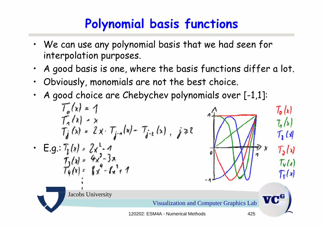
Polynomial basis functions• We can use any polynomial basis that we had seen for
interpolation purposes. • A good basis is one, where the basis functions differ a lot. • Obviously, monomials are not the best choice.• A good choice are Chebychev polynomials over [-1,1]:
• E.g.:
120202: ESM4A - Numerical Methods 426
Visualization and Computer Graphics LabJacobs University
Polynomial regression
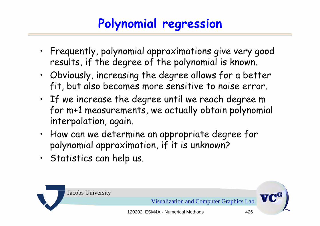
• Frequently, polynomial approximations give very good results, if the degree of the polynomial is known.
• Obviously, increasing the degree allows for a betterfit, but also becomes more sensitive to noise error.
• If we increase the degree until we reach degree m for m+1 measurements, we actually obtain polynomialinterpolation, again.
• How can we determine an appropriate degree forpolynomial approximation, if it is unknown?
• Statistics can help us.
120202: ESM4A - Numerical Methods 427
Visualization and Computer Graphics LabJacobs University
Polynomial regression
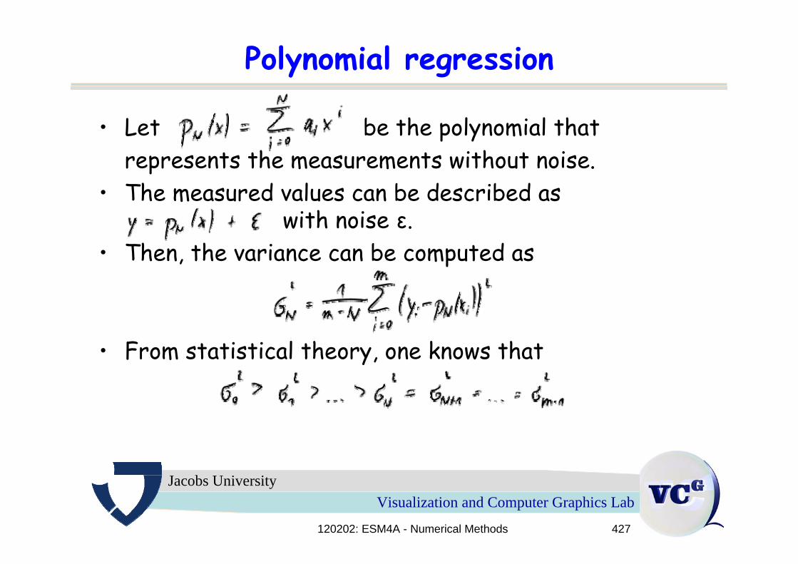
• Let be the polynomial thatrepresents the measurements without noise.
• The measured values can be described as with noise ε.
• Then, the variance can be computed as
• From statistical theory, one knows that
120202: ESM4A - Numerical Methods 428
Visualization and Computer Graphics LabJacobs University
Polynomial regression
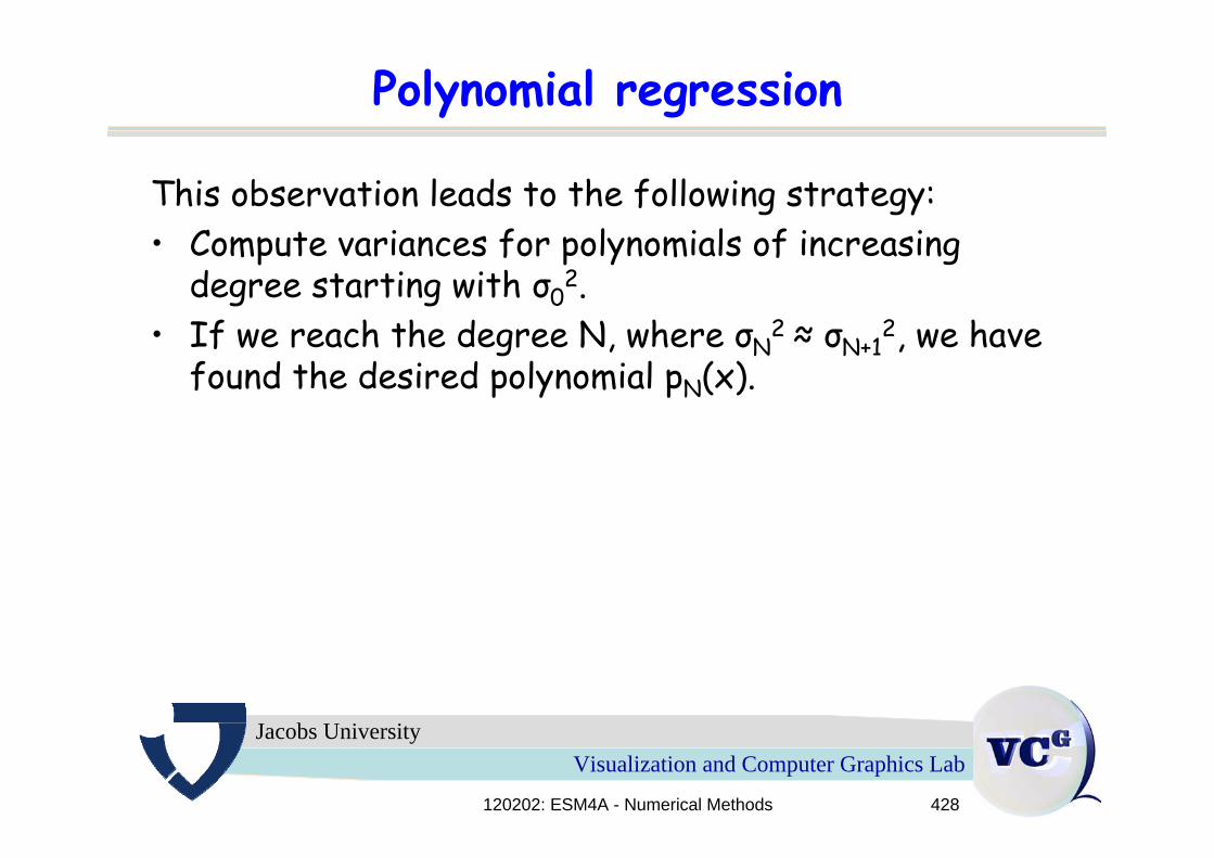
This observation leads to the following strategy:• Compute variances for polynomials of increasing
degree starting with σ02.
• If we reach the degree N, where σN2 ≈ σN+1
2, we havefound the desired polynomial pN(x).
120202: ESM4A - Numerical Methods 429
Visualization and Computer Graphics LabJacobs University
Polynomial regression
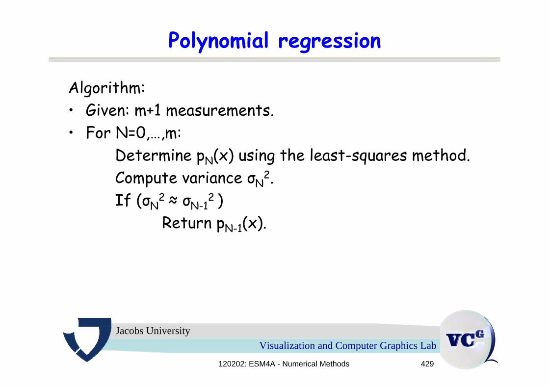
Algorithm:• Given: m+1 measurements.• For N=0,…,m:
Determine pN(x) using the least-squares method.Compute variance σN
2.If (σN
2 ≈ σN-12 )
Return pN-1(x).
120202: ESM4A - Numerical Methods 430
Visualization and Computer Graphics LabJacobs University
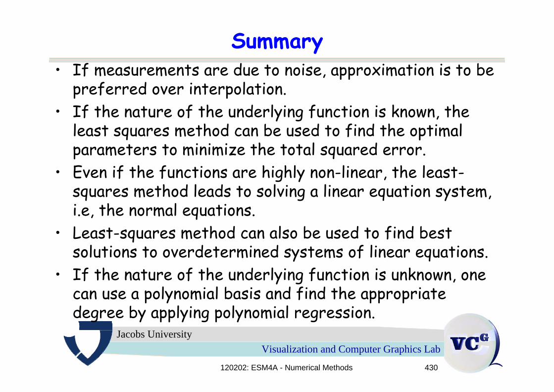
Summary• If measurements are due to noise, approximation is to be
preferred over interpolation.• If the nature of the underlying function is known, the
least squares method can be used to find the optimal parameters to minimize the total squared error.
• Even if the functions are highly non-linear, the least-squares method leads to solving a linear equation system, i.e, the normal equations.
• Least-squares method can also be used to find best solutions to overdetermined systems of linear equations.
• If the nature of the underlying function is unknown, onecan use a polynomial basis and find the appropriatedegree by applying polynomial regression.

120202: ESM4A - Numerical Methods 493
Visualization and Computer Graphics LabJacobs University
5.9 Simpson‘s Scheme
120202: ESM4A - Numerical Methods 494
Visualization and Computer Graphics LabJacobs University
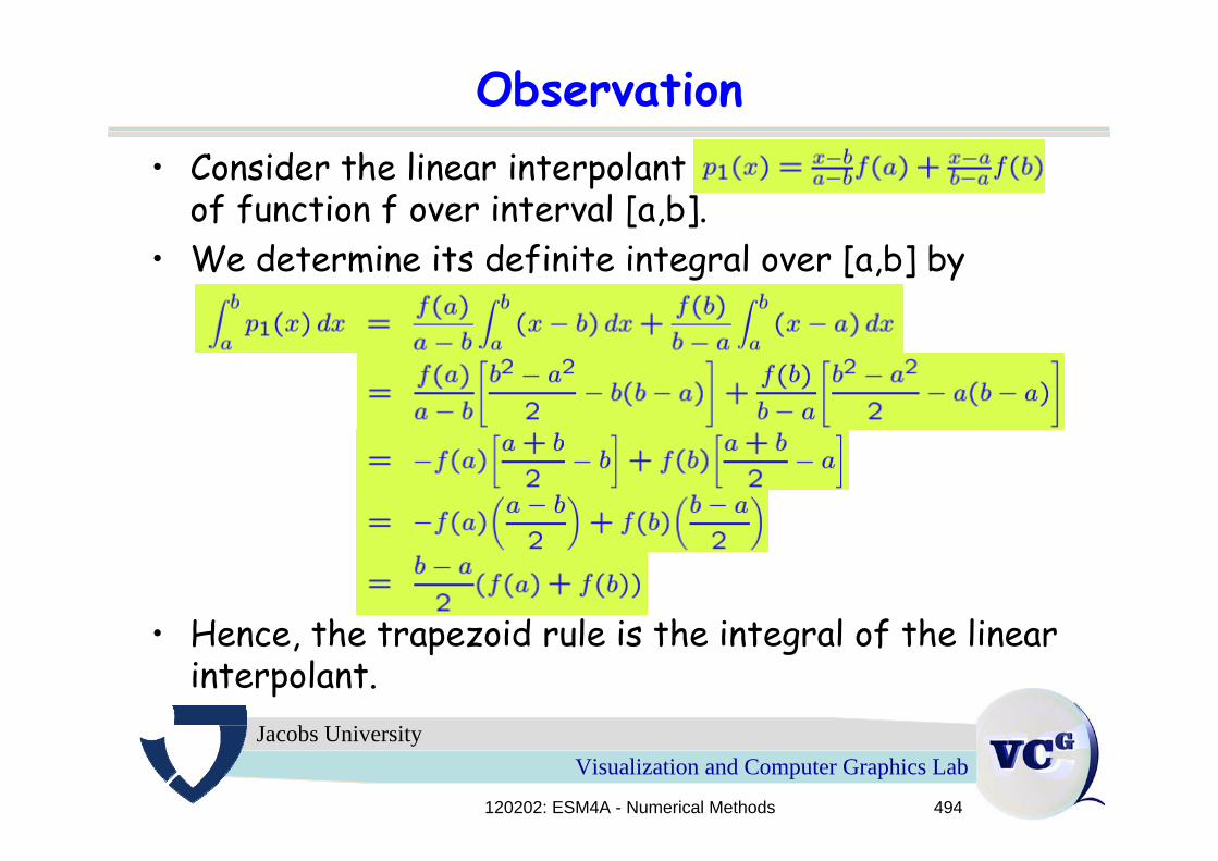
Observation• Consider the linear interpolant
of function f over interval [a,b]. • We determine its definite integral over [a,b] by
• Hence, the trapezoid rule is the integral of the linear interpolant.
120202: ESM4A - Numerical Methods 495
Visualization and Computer Graphics LabJacobs University
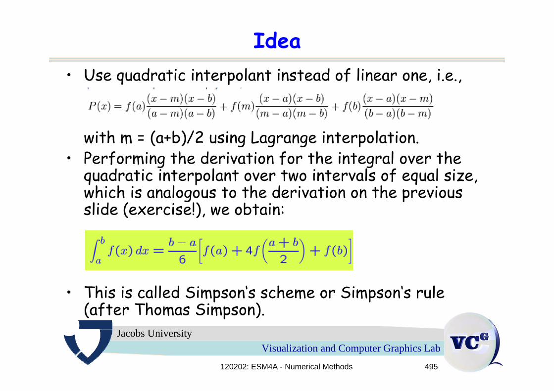
Idea• Use quadratic interpolant instead of linear one, i.e.,
with m = (a+b)/2 using Lagrange interpolation.• Performing the derivation for the integral over the
quadratic interpolant over two intervals of equal size, which is analogous to the derivation on the previousslide (exercise!), we obtain:
• This is called Simpson‘s scheme or Simpson‘s rule(after Thomas Simpson).
120202: ESM4A - Numerical Methods 496
Visualization and Computer Graphics LabJacobs University
Remark
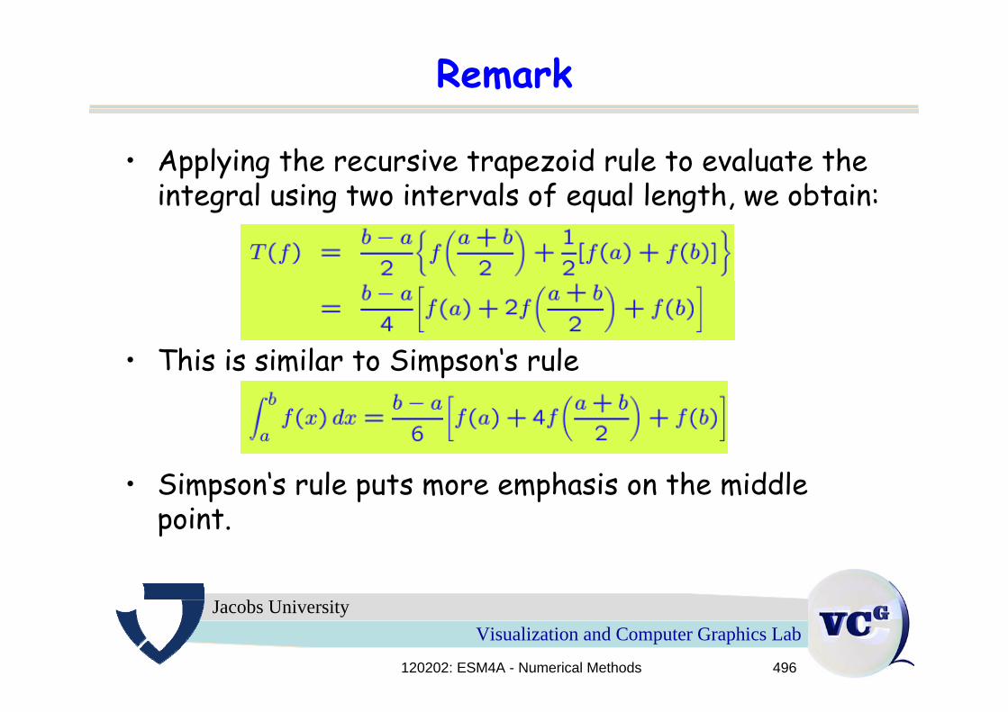
• Applying the recursive trapezoid rule to evaluate theintegral using two intervals of equal length, we obtain:
• This is similar to Simpson‘s rule
• Simpson‘s rule puts more emphasis on the middlepoint.
120202: ESM4A - Numerical Methods 497
Visualization and Computer Graphics LabJacobs University
Error theorem
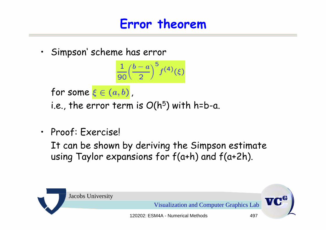
• Simpson‘ scheme has error
for some ,i.e., the error term is O(h5) with h=b-a.
• Proof: Exercise!It can be shown by deriving the Simpson estimateusing Taylor expansions for f(a+h) and f(a+2h).
120202: ESM4A - Numerical Methods 498
Visualization and Computer Graphics LabJacobs University
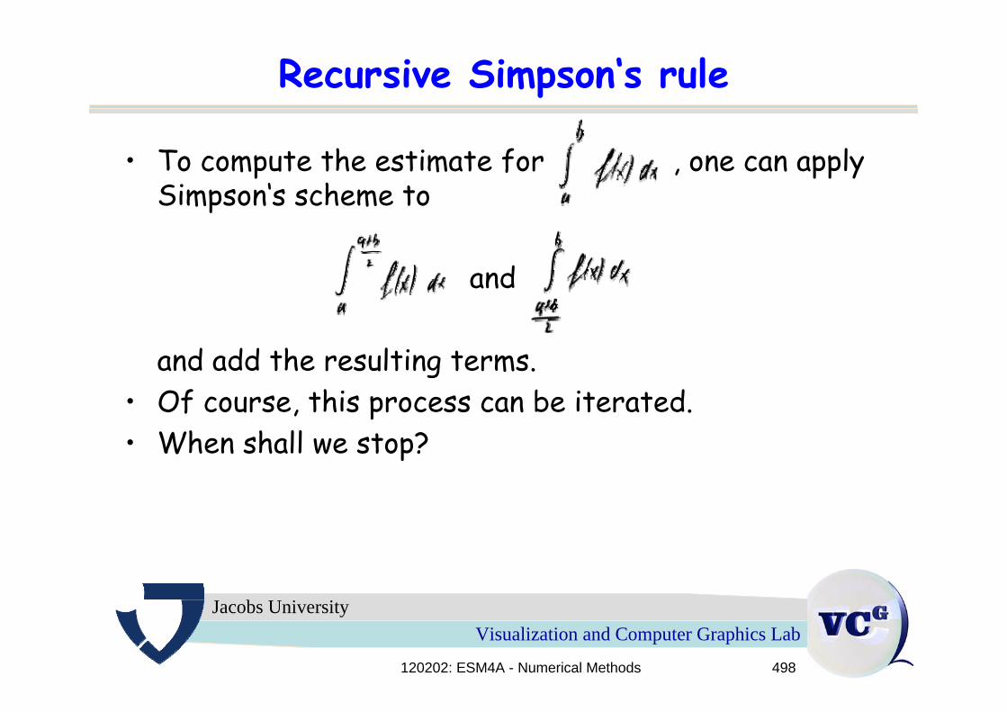
Recursive Simpson‘s rule
• To compute the estimate for , one can applySimpson‘s scheme to
and
and add the resulting terms.• Of course, this process can be iterated.• When shall we stop?
120202: ESM4A - Numerical Methods 499
Visualization and Computer Graphics LabJacobs University
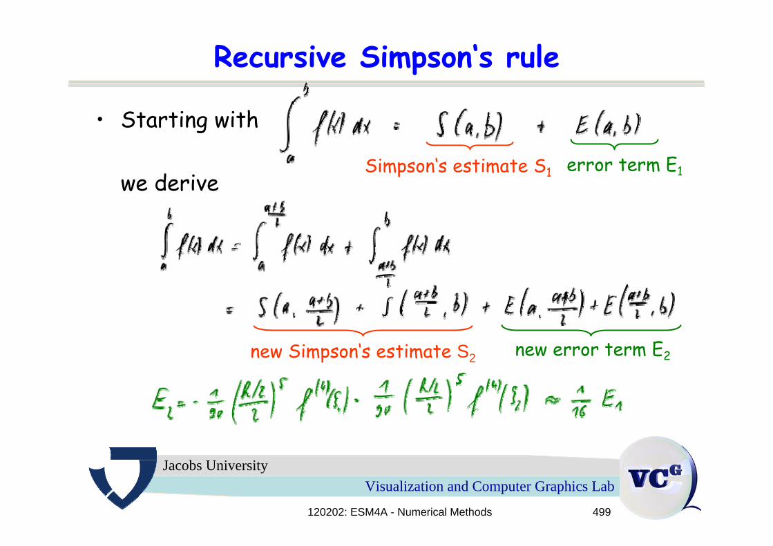
Recursive Simpson‘s rule
• Starting with
we derive
new Simpson‘s estimate S2 new error term E2
Simpson‘s estimate S1 error term E1
120202: ESM4A - Numerical Methods 500
Visualization and Computer Graphics LabJacobs University
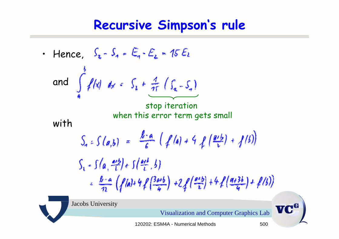
Recursive Simpson‘s rule
• Hence,
and
with
stop iterationwhen this error term gets small
120202: ESM4A - Numerical Methods 501
Visualization and Computer Graphics LabJacobs University
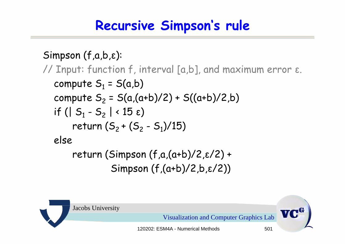
Recursive Simpson‘s rule
Simpson (f,a,b,ε):// Input: function f, interval [a,b], and maximum error ε.
compute S1 = S(a,b)compute S2 = S(a,(a+b)/2) + S((a+b)/2,b)if (| S1 - S2 | < 15 ε)
return (S2 + (S2 - S1)/15)else
return (Simpson (f,a,(a+b)/2,ε/2) + Simpson (f,(a+b)/2,b,ε/2))
120202: ESM4A - Numerical Methods 502
Visualization and Computer Graphics LabJacobs University
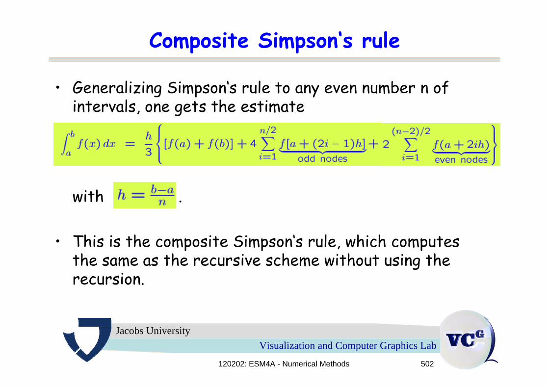
Composite Simpson‘s rule
• Generalizing Simpson‘s rule to any even number n of intervals, one gets the estimate
with .
• This is the composite Simpson‘s rule, which computesthe same as the recursive scheme without using therecursion.
120202: ESM4A - Numerical Methods 503
Visualization and Computer Graphics LabJacobs University
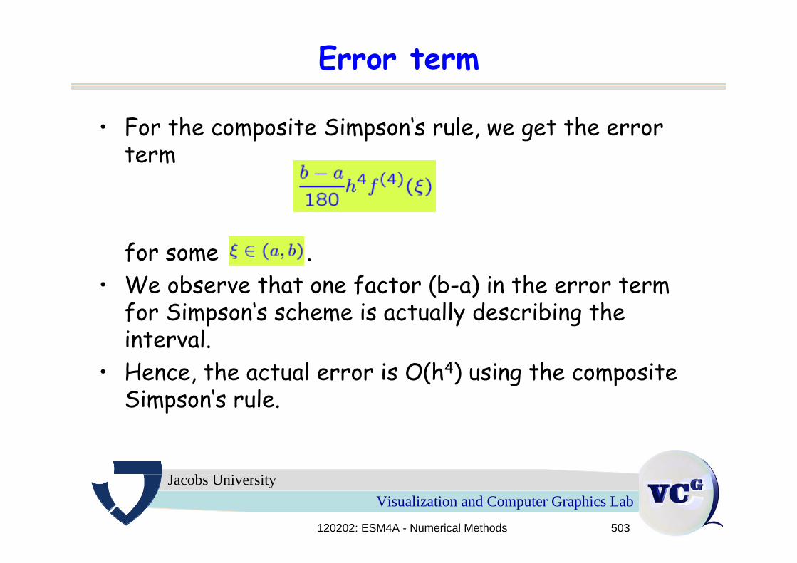
Error term
• For the composite Simpson‘s rule, we get the errorterm
for some .• We observe that one factor (b-a) in the error term
for Simpson‘s scheme is actually describing theinterval.
• Hence, the actual error is O(h4) using the compositeSimpson‘s rule.
120202: ESM4A - Numerical Methods 504
Visualization and Computer Graphics LabJacobs University
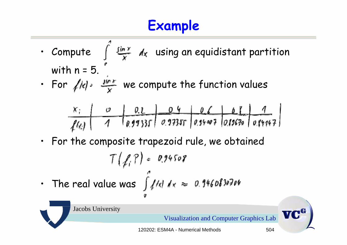
Example
• Compute using an equidistant partition
with n = 5. • For we compute the function values
• For the composite trapezoid rule, we obtained
• The real value was
120202: ESM4A - Numerical Methods 505
Visualization and Computer Graphics LabJacobs University
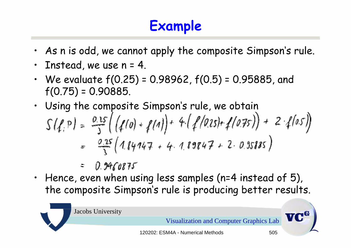
Example
• As n is odd, we cannot apply the composite Simpson‘s rule.• Instead, we use n = 4.• We evaluate f(0.25) = 0.98962, f(0.5) = 0.95885, and
f(0.75) = 0.90885.• Using the composite Simpson‘s rule, we obtain
• Hence, even when using less samples (n=4 instead of 5), the composite Simpson‘s rule is producing better results.
120202: ESM4A - Numerical Methods 506
Visualization and Computer Graphics LabJacobs University
Remark
• The error term using the composite Simpson‘s rulehas better behavior that the one using the compositetrapezoid rule.
• However, both schemes apply about the samecomputations (just weighted differently).
• As we did in the Romberg algorithm for the compositetrapezoid rule, one can also apply Richardsenextrapolation to the composite Simpson‘s rule to obtain even better error terms.
120202: ESM4A - Numerical Methods 507
Visualization and Computer Graphics LabJacobs University
5.10 Gaussian Quadrature
120202: ESM4A - Numerical Methods 508
Visualization and Computer Graphics LabJacobs University
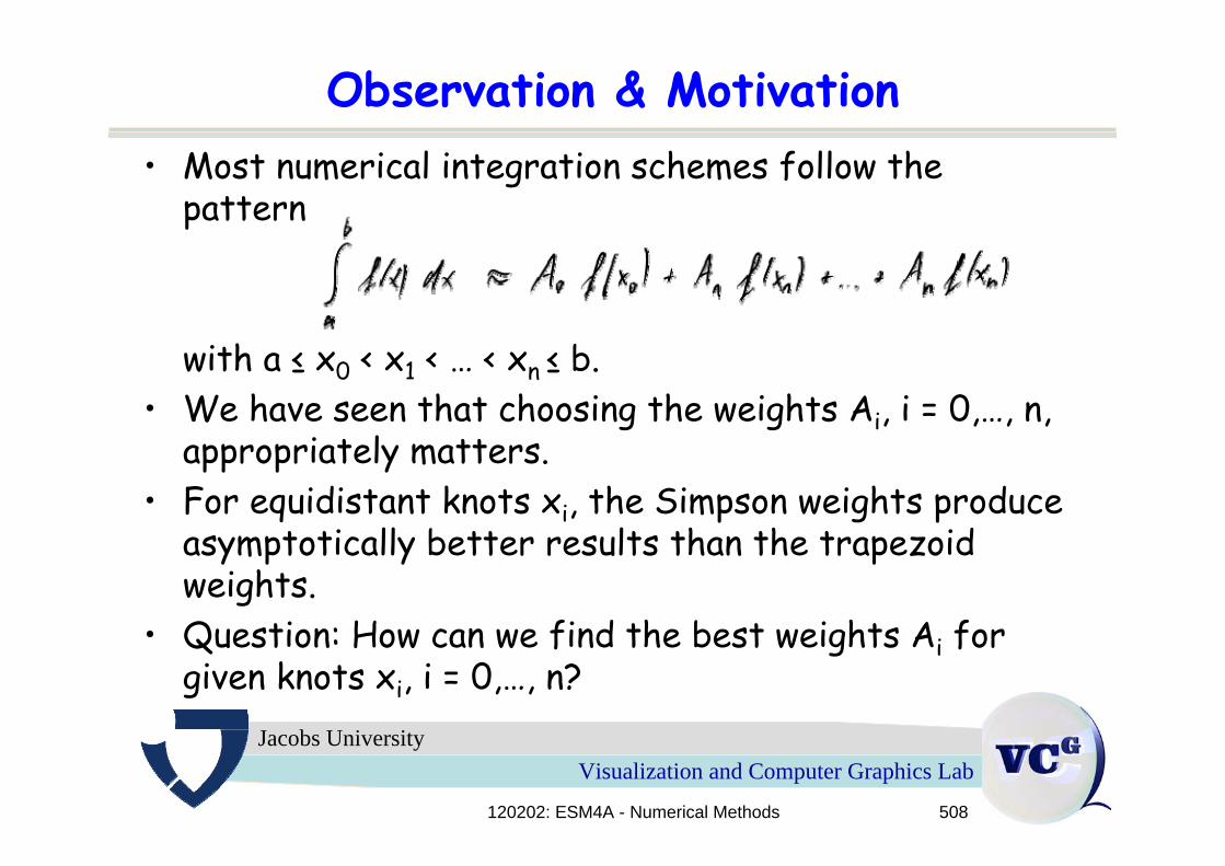
Observation & Motivation• Most numerical integration schemes follow the
pattern
with a ≤ x0 < x1 < … < xn ≤ b.• We have seen that choosing the weights Ai, i = 0,…, n,
appropriately matters.• For equidistant knots xi, the Simpson weights produce
asymptotically better results than the trapezoidweights.
• Question: How can we find the best weights Ai forgiven knots xi, i = 0,…, n?
120202: ESM4A - Numerical Methods 509
Visualization and Computer Graphics LabJacobs University
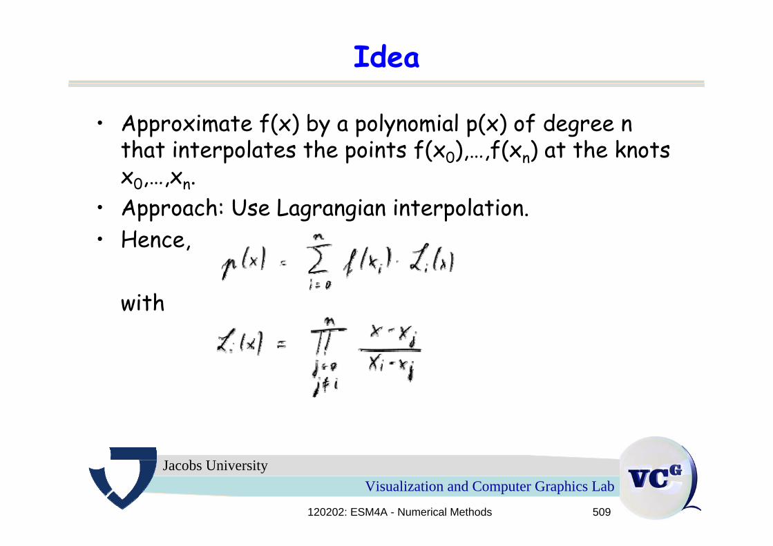
Idea
• Approximate f(x) by a polynomial p(x) of degree n that interpolates the points f(x0),…,f(xn) at the knotsx0,…,xn.
• Approach: Use Lagrangian interpolation.• Hence,
with
120202: ESM4A - Numerical Methods 510
Visualization and Computer Graphics LabJacobs University
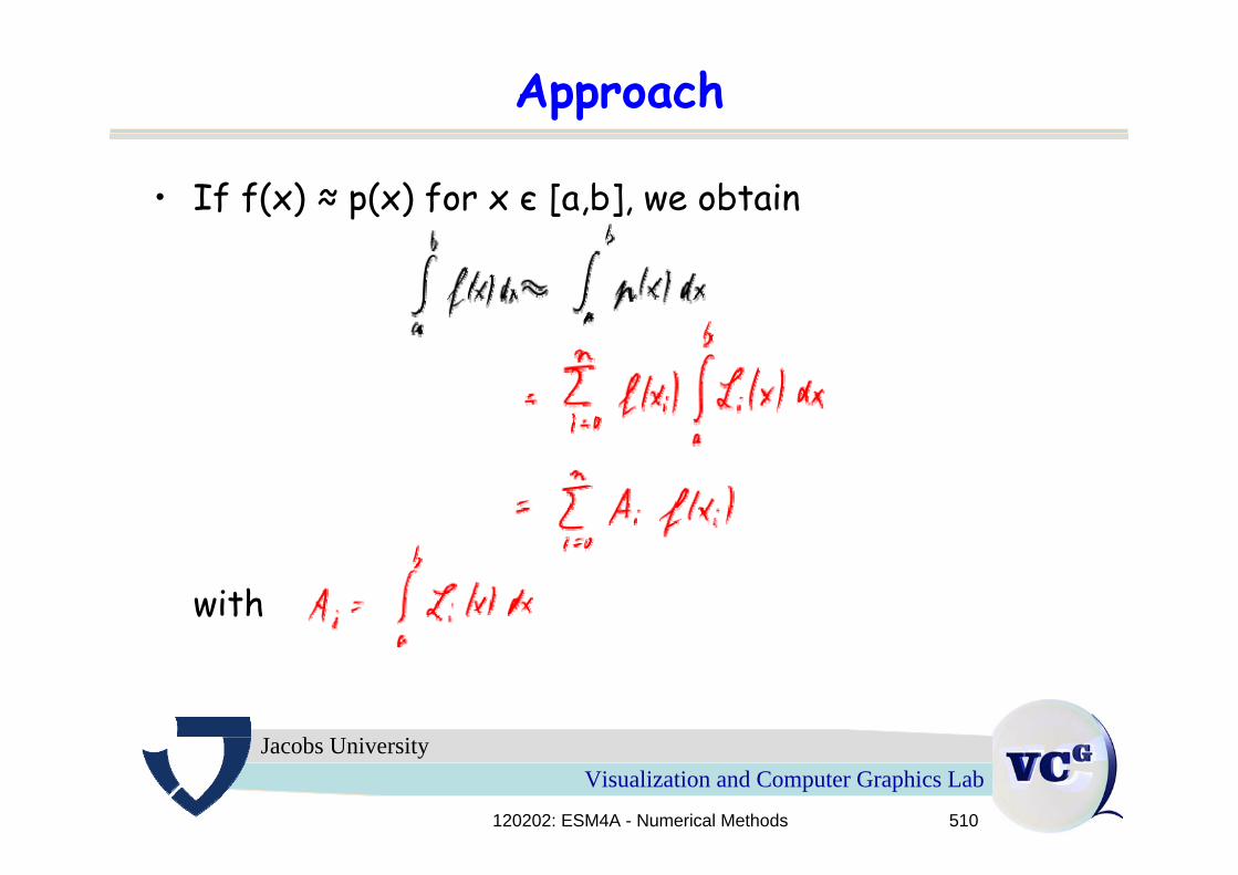
Approach
• If f(x) ≈ p(x) for x є [a,b], we obtain
with
120202: ESM4A - Numerical Methods 511
Visualization and Computer Graphics LabJacobs University
Remark
• The weights Ai only depend on the knot sequencex0,…,xn, but are independent of the function f(x) wewant to integrate.
• Hence, for a given knot sequence, the Ai can beprecomputed and stored.
• During integration, the Ai are multiplied with thefunction values f(xi) and the products are summed up.
120202: ESM4A - Numerical Methods 512
Visualization and Computer Graphics LabJacobs University
Remark
• This is a generalization of the trapezoid rule and theSimpson‘s rule, as we had seen that they can bederived as the integral over the linear and quadraticpolynomials, respectively, (also using Lagrangeinterpolation).
120202: ESM4A - Numerical Methods 513
Visualization and Computer Graphics LabJacobs University
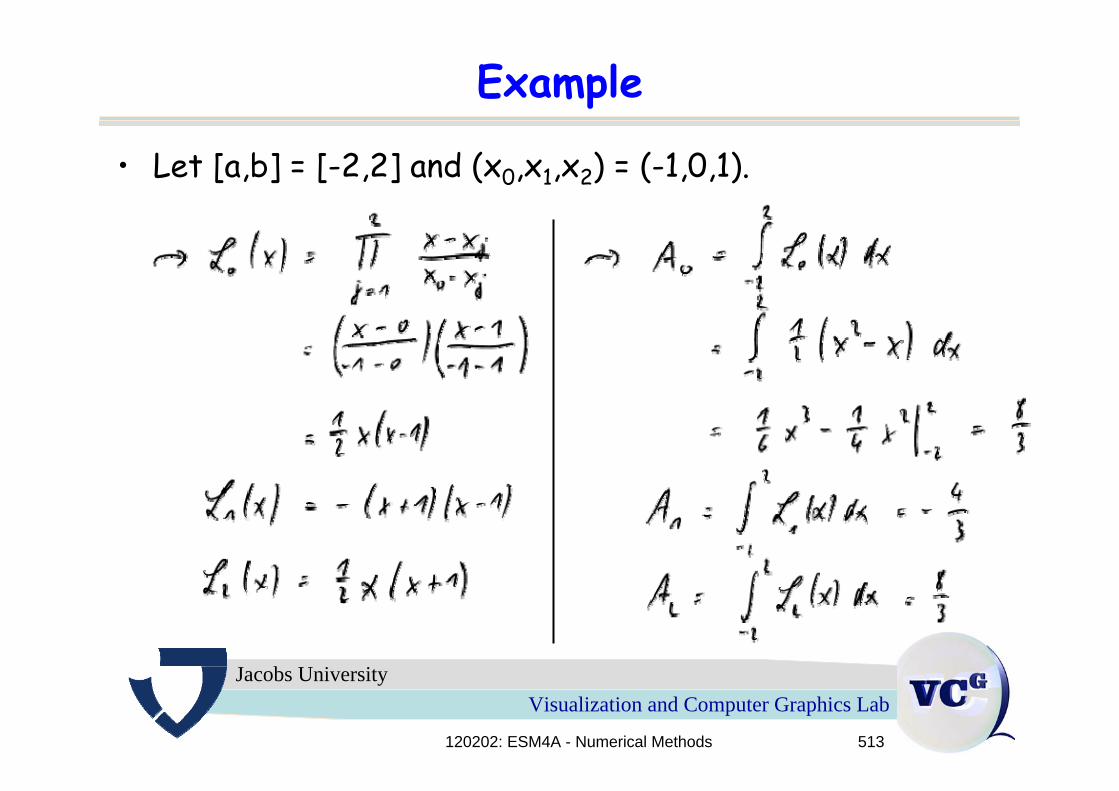
Example
• Let [a,b] = [-2,2] and (x0,x1,x2) = (-1,0,1).
120202: ESM4A - Numerical Methods 514
Visualization and Computer Graphics LabJacobs University
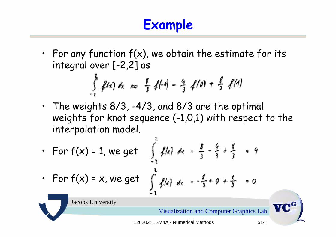
Example
• For any function f(x), we obtain the estimate for itsintegral over [-2,2] as
• The weights 8/3, -4/3, and 8/3 are the optimal weights for knot sequence (-1,0,1) with respect to theinterpolation model.
• For f(x) = 1, we get
• For f(x) = x, we get
120202: ESM4A - Numerical Methods 515
Visualization and Computer Graphics LabJacobs University
Remark
• If f is a polynomial of degree ≤ n, we have f(x) = p(x).• Consequently, the integration scheme is exact.• This is true for any knot sequence with n+1 knots.• How about if f is a polynomial of degree > n?
120202: ESM4A - Numerical Methods 516
Visualization and Computer Graphics LabJacobs University
Gaussian quadrature
• Up to now, we assumed that the knots x0,…,xn aregiven.
• They can actually be arbitrary.• For practical reasons, it makes sense to postulate
that they belong to interval [a,b].• Karl Friedrich Gauß (1777-1855) discovered that wise
placement of the knots can significantly improve theaccuracy of the numerical integration scheme.
• He formulated the choice of the special placement in the Gaussian quadrature theorem, where quadratureis another term for integration.
120202: ESM4A - Numerical Methods 517
Visualization and Computer Graphics LabJacobs University
Gaussian quadrature theorem
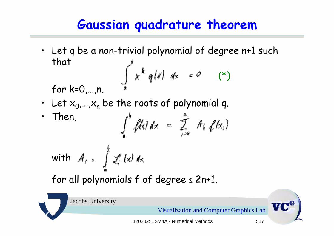
• Let q be a non-trivial polynomial of degree n+1 such that
(*)for k=0,…,n.
• Let x0,…,xn be the roots of polynomial q.• Then,
with
for all polynomials f of degree ≤ 2n+1.
120202: ESM4A - Numerical Methods 518
Visualization and Computer Graphics LabJacobs University
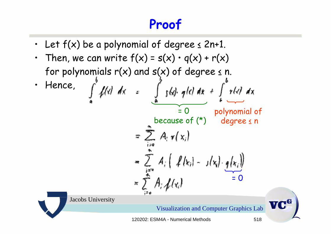
Proof• Let f(x) be a polynomial of degree ≤ 2n+1.• Then, we can write f(x) = s(x) • q(x) + r(x)
for polynomials r(x) and s(x) of degree ≤ n.• Hence,
= 0 because of (*)
polynomial of degree ≤ n
= 0
120202: ESM4A - Numerical Methods 519
Visualization and Computer Graphics LabJacobs University
Remark
• The n+1 equations (*) do not define the polynomialq(x) uniquely, as q(x) is of degree n+1, i.e., it has n+2 coefficients in a monomial representation.
120202: ESM4A - Numerical Methods 520
Visualization and Computer Graphics LabJacobs University
Gaussian quadrature
• Following the Gaussian quadrature theorem, we fix the n+1 knots x0,…,xn.
• The knots are also referred to as Gaussian nodes.• The knots uniquely determine the polynomial p(x) that
is supposed to approximate function f(x).• Having determined the knots, we use Lagrangian
interpolation to obtain the weights A0,…,An.• Altogether, we have chosen 2(n+1) variables to find an
optimal estimate for the integral (when using n+1 knots).
• This integration scheme is called Gaussianquadrature.
120202: ESM4A - Numerical Methods 521
Visualization and Computer Graphics LabJacobs University
Remark
• We had figured out that the choice of weightsA0,…,An does only depend on the knots x0,…,xn.
• Using Gaussian quadrature, also the choice of theknots x0,…,xn is independent of the function f(x) wewant to integrate.
• Both knots x0,…,xn and weights A0,…,An aredetermined by the degree n of polynomial p(x) and the integration interval [a,b].
• Hence, all 2(n+1) parameters x0,…,xn and A0,…,An canbe precomputed independently of function f(x).
120202: ESM4A - Numerical Methods 522
Visualization and Computer Graphics LabJacobs University
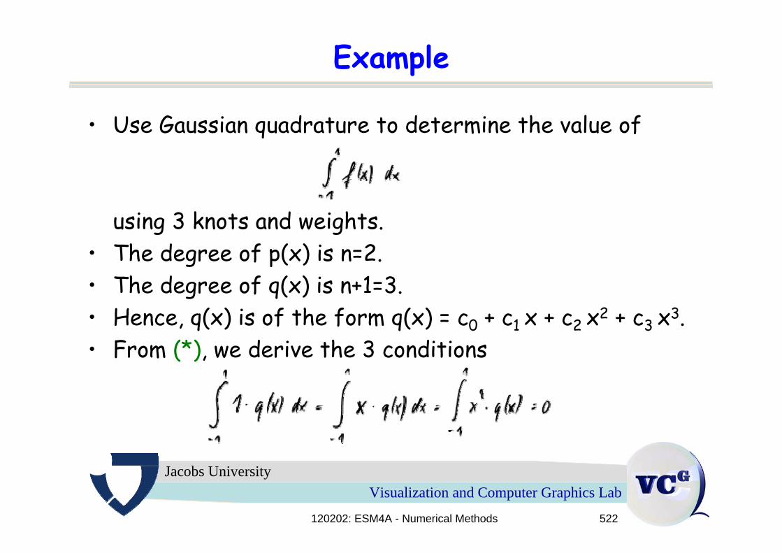
Example
• Use Gaussian quadrature to determine the value of
using 3 knots and weights.• The degree of p(x) is n=2.• The degree of q(x) is n+1=3.• Hence, q(x) is of the form q(x) = c0 + c1 x + c2 x2 + c3 x3.• From (*), we derive the 3 conditions
120202: ESM4A - Numerical Methods 523
Visualization and Computer Graphics LabJacobs University
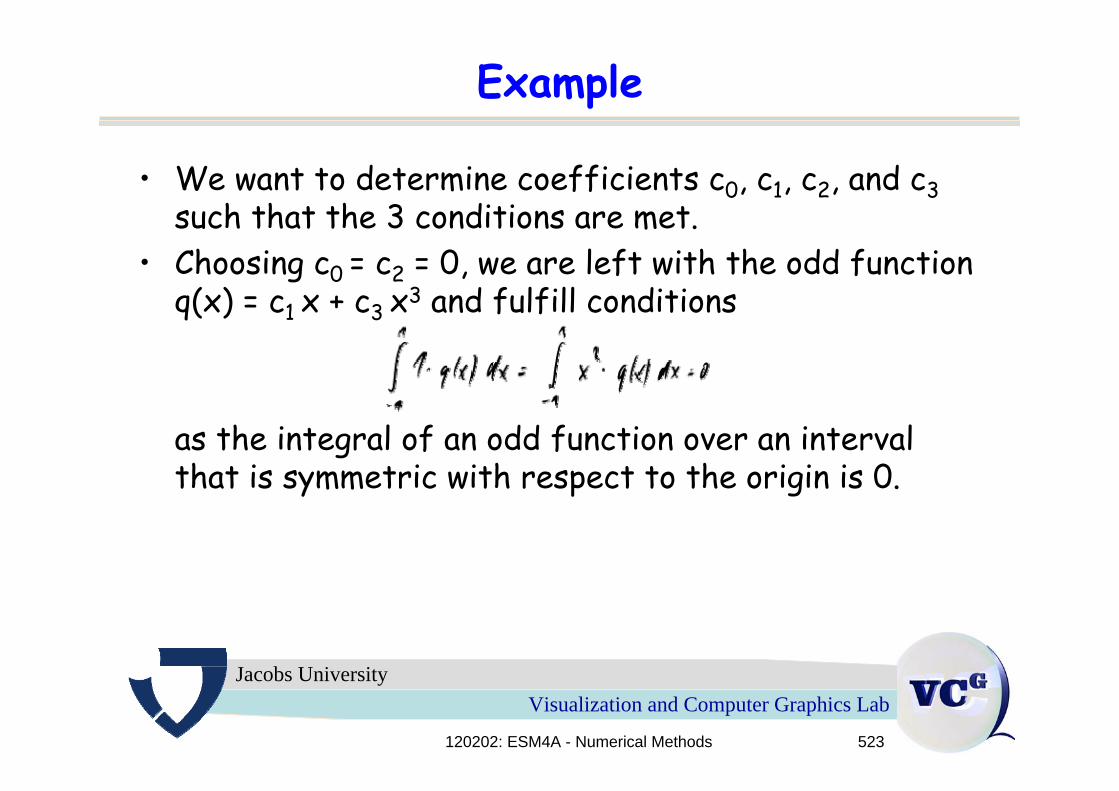
Example
• We want to determine coefficients c0, c1, c2, and c3 such that the 3 conditions are met.
• Choosing c0 = c2 = 0, we are left with the odd functionq(x) = c1 x + c3 x3 and fulfill conditions
as the integral of an odd function over an intervalthat is symmetric with respect to the origin is 0.
120202: ESM4A - Numerical Methods 524
Visualization and Computer Graphics LabJacobs University
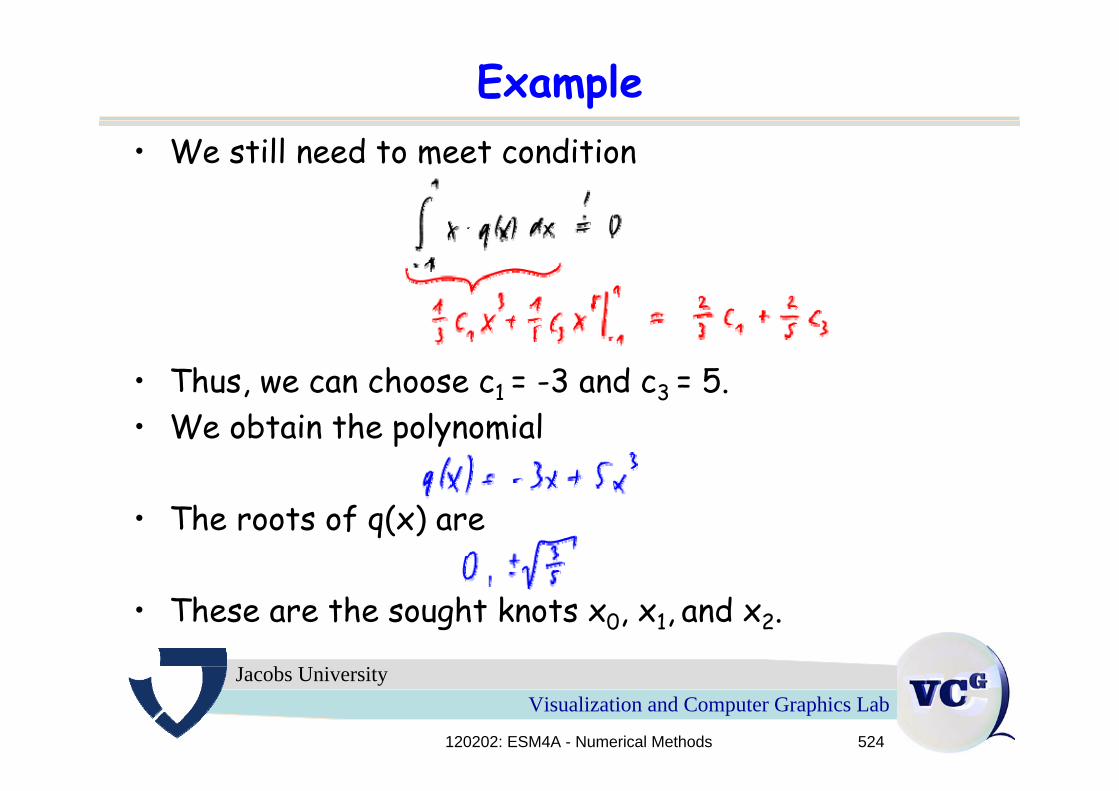
Example• We still need to meet condition
• Thus, we can choose c1 = -3 and c3 = 5.• We obtain the polynomial
• The roots of q(x) are
• These are the sought knots x0, x1, and x2.
120202: ESM4A - Numerical Methods 525
Visualization and Computer Graphics LabJacobs University
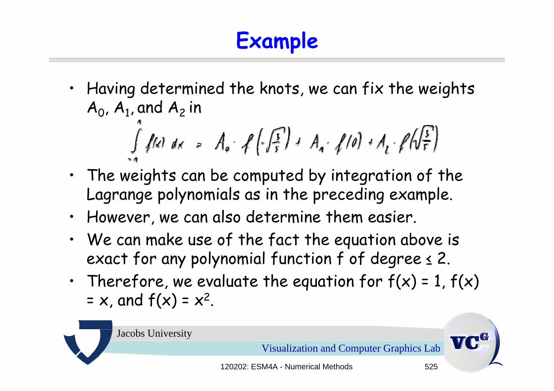
Example
• Having determined the knots, we can fix the weightsA0, A1, and A2 in
• The weights can be computed by integration of theLagrange polynomials as in the preceding example.
• However, we can also determine them easier.• We can make use of the fact the equation above is
exact for any polynomial function f of degree ≤ 2.• Therefore, we evaluate the equation for f(x) = 1, f(x)
= x, and f(x) = x2.
120202: ESM4A - Numerical Methods 526
Visualization and Computer Graphics LabJacobs University
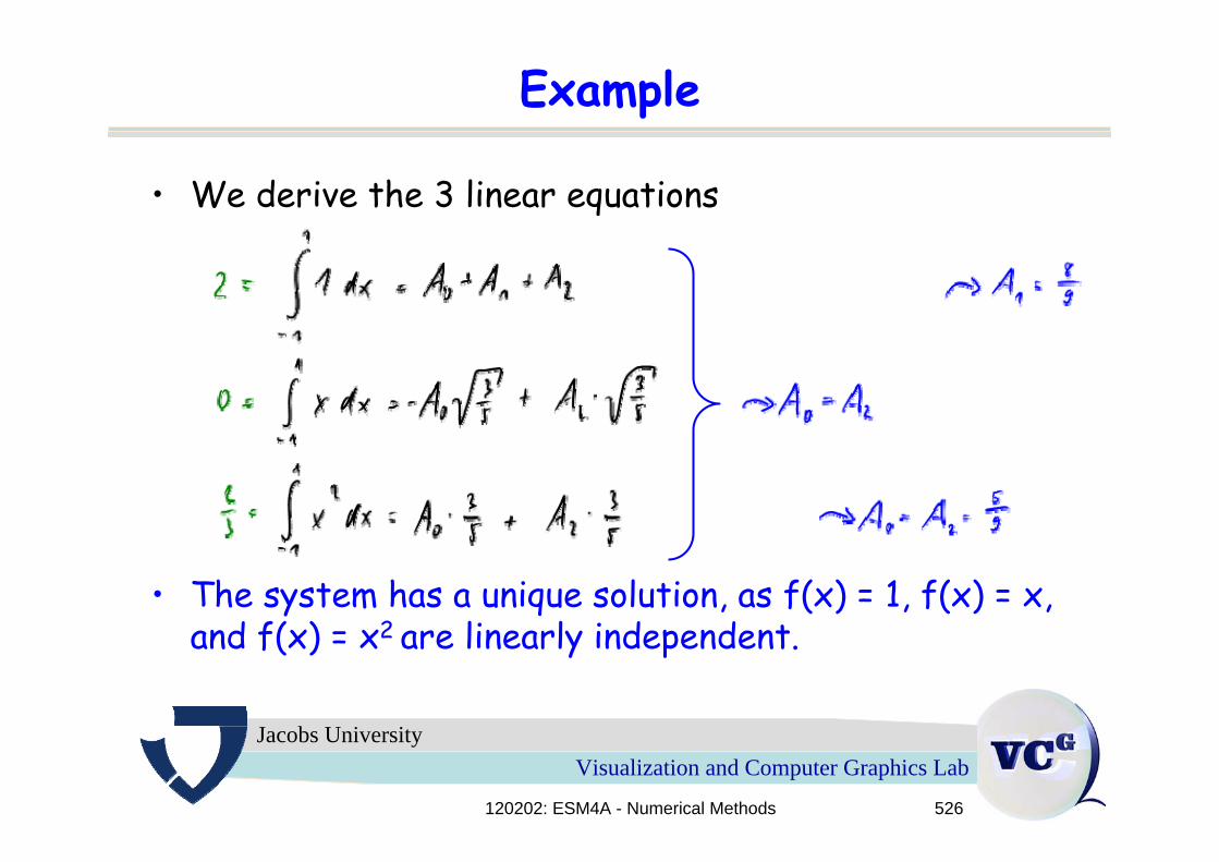
Example
• We derive the 3 linear equations
• The system has a unique solution, as f(x) = 1, f(x) = x, and f(x) = x2 are linearly independent.
120202: ESM4A - Numerical Methods 527
Visualization and Computer Graphics LabJacobs University
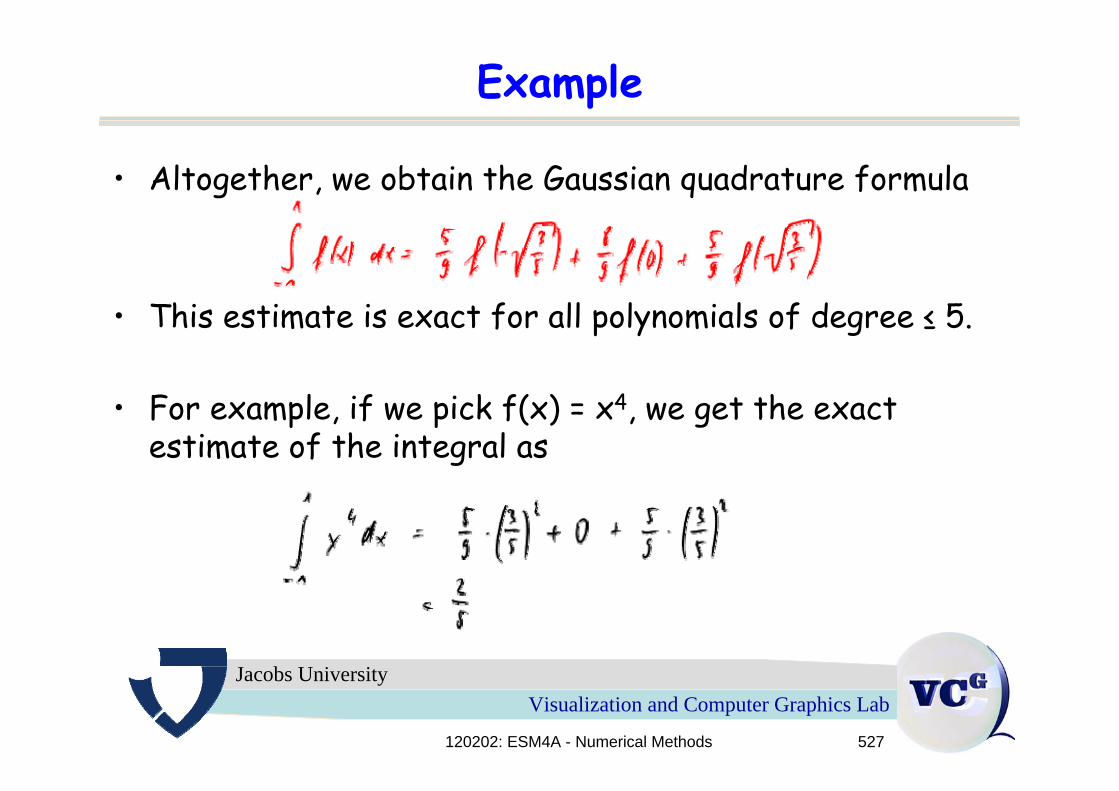
Example
• Altogether, we obtain the Gaussian quadrature formula
• This estimate is exact for all polynomials of degree ≤ 5.
• For example, if we pick f(x) = x4, we get the exactestimate of the integral as
120202: ESM4A - Numerical Methods 528
Visualization and Computer Graphics LabJacobs University
Interval transformation
• The only input to computing Gaussian nodes and weights was the interval [-1,1] and the number of Gaussian nodes.
• Question: Can we use this result to compute integralsover a different interval?
• Can we use the result to compute the integral overany interval [a,b]?
120202: ESM4A - Numerical Methods 529
Visualization and Computer Graphics LabJacobs University
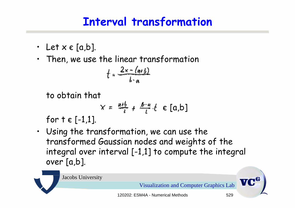
Interval transformation
• Let x є [a,b].• Then, we use the linear transformation
to obtain thatє [a,b]
for t є [-1,1].• Using the transformation, we can use the
transformed Gaussian nodes and weights of theintegral over interval [-1,1] to compute the integral over [a,b].
120202: ESM4A - Numerical Methods 530
Visualization and Computer Graphics LabJacobs University
Interval transformation
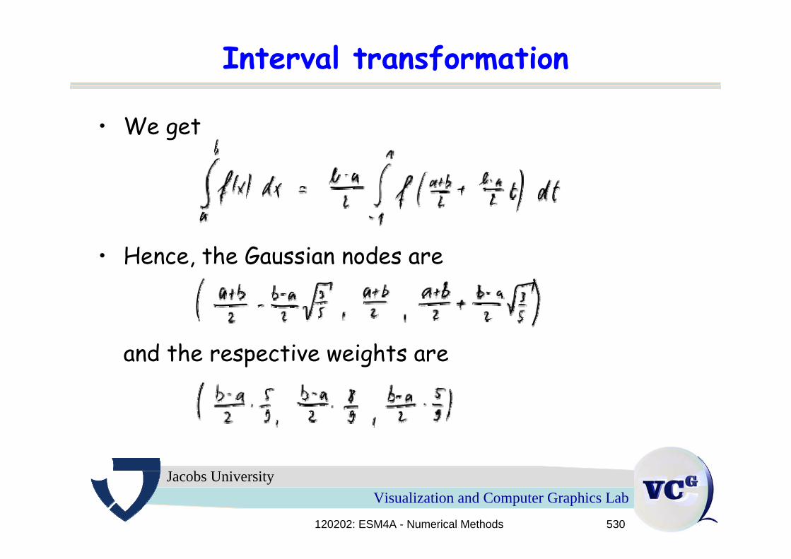
• We get
• Hence, the Gaussian nodes are
and the respective weights are
120202: ESM4A - Numerical Methods 531
Visualization and Computer Graphics LabJacobs University
Example
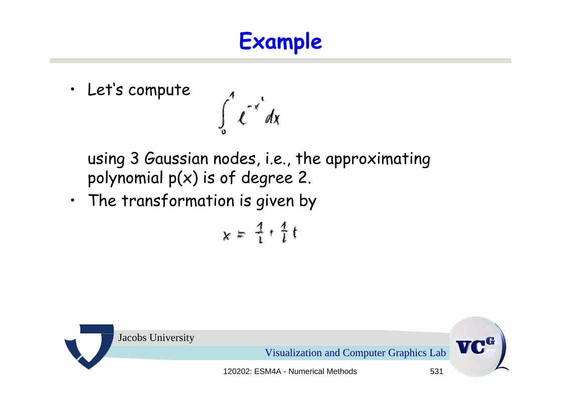
• Let‘s compute
using 3 Gaussian nodes, i.e., the approximatingpolynomial p(x) is of degree 2.
• The transformation is given by
120202: ESM4A - Numerical Methods 532
Visualization and Computer Graphics LabJacobs University
Example
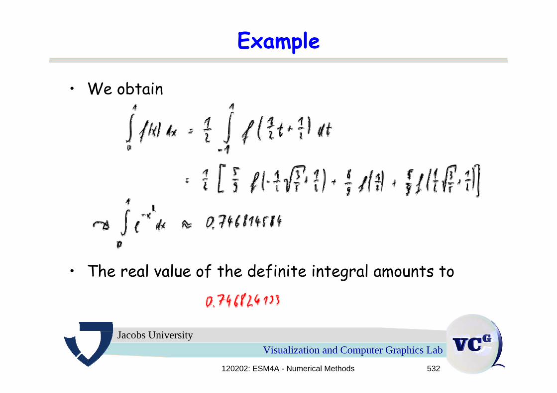
• We obtain
• The real value of the definite integral amounts to
120202: ESM4A - Numerical Methods 533
Visualization and Computer Graphics LabJacobs University
Polynomial q(x)
• We have seen that polynomial q(x) was of degree n+1, where n was the degree of the approximatingpolynomial n.
• From (*), we derive n+1 conditions, which left us withone degree of freedom for choosing polynomial q(x).
• If we “normalize“ polynomial q(x) by postulating thatq(1) = 1, we obtain a unique representation of q(x).
• Considering the interval [-1,1], the resultingpolynomials are called Legendre polynomials.
• They are named after Adrien-Marie Legendre (1752-1833).
120202: ESM4A - Numerical Methods 534
Visualization and Computer Graphics LabJacobs University
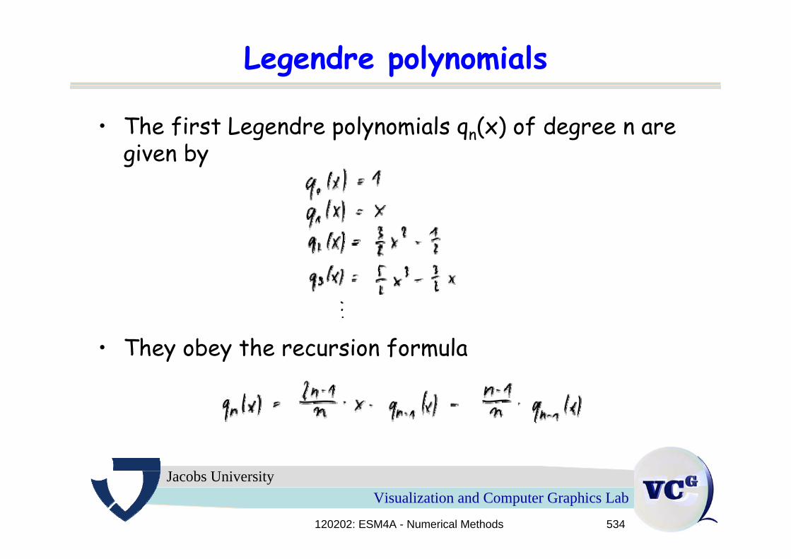
Legendre polynomials
• The first Legendre polynomials qn(x) of degree n aregiven by
• They obey the recursion formula


![Notes on Polynomial Functors - UAB Barcelonakock/cat/polynomial.pdf · 2018. 1. 11. · • Polynomial functors and polynomial monads [39] with Gambino • Polynomial functors and](https://img.pdfslide.net/doc/110x75/60faf8a63b5d714a860ca184/notes-on-polynomial-functors-uab-barcelona-kockcat-2018-1-11-a-polynomial.jpg)