Polynomial Interpolation to Data on Flats in Rd general interpolation problem is analysed in Section 7. Some simple facts, concerning D-invariant polynomial subspaces, especially polynomial

Journal of Approximation Theory 105, 313�343 (2000)

Polynomial Interpolation to Data on Flats in Rd

Carl de Boor

Department of Computer Sciences, University of Wisconsin-Madison,1210 West Dayton Street, Madison,

Wisconsin 53706, U.S.A.

Nira Dyn

School of Mathematical Sciences, Tel-Aviv University, Ramat-Aviv, 69978, Tel-Aviv, Israel

and

Amos Ron

Department of Computer Sciences, University of Wisconsin-Madison,1210 West Dayton Street, Madison,

Wisconsin 53706, U.S.A.

Communicated by Borislav Bojanov

Received September 9, 1999; accepted February 25, 2000

Stimulated by recent work of Hakopian and Sahakian, polynomial interpolationto data at all the s-dimensional intersections of an arbitrary sequence ofhyperplanes in Rd is considered, and reduced, by the adjunction of an additional shyperplanes in general position with respect to the given sequence, to the case s=0solved much earlier by two of the present authors. In particular, interpolation isfrom the very same polynomial spaces already used earlier. The difficult question ofmultiplicity and corresponding matching of derivative information is completelysolved, with the number of independent derivative conditions at an intersectionexactly equal to that intersection's multiplicity. Also, the consistency requirementsplaced on the data are minimal in the sense that they need to be checked only atthe finitely many 0-dimensional intersections of the hyperplanes involved. Thearguments used provide, incidentally, further insights into the two polynomialspaces, P(5) and D(5), of basic interest in box spline theory. � 2000 Academic Press

Key Words: polynomial interpolation; multivariate; linear manifold; box splinetheory.

doi:10.1006�jath.2000.3473, available online at http:��www.idealibrary.com on

3130021-9045�00 �35.00

Copyright � 2000 by Academic PressAll rights of reproduction in any form reserved.

This research was supported in part by the United States Army (DAAL03-G-90-0090,DAAH04-95-1-0089, DAAG55-98-1-0443), and by the National Science Foundation (GrantsDMS-9000053, DMS-9224748, DMS-9626319).

1. INTRODUCTION

When going from univariate to multivariate polynomial interpolation,one can follow the point of view of [HS2] that a point in R=R1

corresponds to a hyperplane in Rd and, correspondingly, attempt to inter-polate to information given on hyperplanes. It is one message of the presentpaper that the efficient way to solve such interpolation problems isnevertheless via an equivalent problem of interpolation to (derived) infor-mation given at points. The relevant pointset is obtained as the set of all0-dimensional intersections of hyperplanes from the set that comprises thegiven hyperplanes and d&1 additional hyperplanes in general position.Interpolation at such pointsets was studied already in [DR].

In [DR, BDR], we considered interpolation problems in which twopolynomial spaces that emerge from box spline theory, P(5) and D(5), areinvolved. Usually, one of these spaces is used to determine the interpolationconditions and the interpolant is sought from the other. In the above-citedpapers, the interpolation conditions are always of Lagrange type orHermite type, i.e., we interpolate function values and ``consecutive''derivative values at these points. Motivated by the recent interesting paper[HS2] of Hakopian and Sahakian, we study in this paper polynomialinterpolation to data given on certain linear manifolds or flats (for short)in Rd, all of the same dimension s, and this dimension is held fixedthroughout. The case s=0 reduces to the interpolation problem consideredin [DR].

The collection of s-dimensional flats involved is denoted by Ms(H); itconsists of all s-dimensional intersections of hyperplanes taken from agiven sequence H.

Generically, each M # Ms(H) is the intersection of exactly d&s hyper-planes, and we call this situation (whether generic or not) the simple case,and expect, in this case, to match values given at all the flats in Ms(H), i.e.,Lagrange type interpolation. The examples shown as Cases 1.1�1.3 inSection 2 are of this type.

In the contrary case (see, e.g., the examples shown as Cases 2.1�2.4 inSection 2), some M # Ms(H) is the intersection of more than d&s hyper-planes, and, correspondingly, we would expect to match at such M alsosome ``successive'' derivatives, leading to Hermite type interpolation.However, in contrast to [HS2], we would not demand the matching of allderivatives up to a certain order. Rather, in a ready generalization of theapproach introduced in [DR], we impose Hermite conditions that can beshown to be exactly those satisfied, in a suitable limiting process, by aLagrange interpolant to data taken from a smooth function. In this way,the resulting Hermite interpolation is osculatory or ``repeated'' interpolationin the classical sense.

314 DE BOOR, DYN, AND RON

Specification of data on flats of dimension s>0 raises the question ofconsistency: Since distinct M, M$ # Ms(H) may well have a nontrivial inter-section, there is the possibility that the information supplied on M and M$is contradictory on M & M$. In the Lagrange case, this is simply a questionof having the two polynomials, specified on M and M$, respectively,coincide on M & M$. In the Hermite case, matters are a bit more subtle.Fortunately, in contrast to [HS2], we are able to reduce all such con-sistency questions to checking consistency at a certain finite set (namely theset M0(Hs); see below).

Given that, even in the simple case, the cardinality of Ms(H) is not justa function of *H, we must also specify a suitable H-dependent polynomialspace from which to interpolate. This was already recognized in [DR]where the case s=0 of our current problem was settled. In fact, ourapproach reduces the general problem to the special case treated in [DR]:we extract from the given data a discrete (finite) set of Hermite type inter-polation conditions, and choose the interpolant from a polynomial spaceP=Ps(H) which depends only on the sequence H and the number s. Wewill not be able to match the information given at all the M # Ms(H) bysome p # P unless the information is compatible with P, i.e., unless thedatum specified on a given M # Ms(H) is taken from some element of P

(with that element, offhand, different from datum to datum).With this, our main result, Theorem 7.19, states that, for an arbitrary

finite sequence H of hyperplanes and arbitrary consistent and P-compatibledata, there is exactly one element p # P that matches these data.

Our proof of this result is quite technical, and provides, perhapsunexpected, insights into the structure of the spaces D(5) which play sucha central role in box spline theory (see, e.g., [BDR]). These insights arecontained in Theorem 7.7 which is a consequence of Theorem 7.9, andin Theorem 7.13. It is our hope that these insights will also find use else-where.

The paper is laid out as follows. All of our functions hereafter are com-plex-valued and defined on Rd. In order to simplify the presentation, weconsider first (in Section 5) the simple case, i.e., the Lagrange type inter-polation that is analysed here. This simplifies almost all aspects of theanalysis: the description of the interpolation conditions, the compatibilityrequirements on the interpolation conditions, and the solution we provideto the interpolation problem. In contrast, the polynomial space that is tosupply the interpolant is the same for the Lagrange and non-Lagrangeproblems, hence we need first to introduce and discuss that space, as we doin (Section 3 and) Section 4.

In Section 2, we illustrate our interpolation problems by treating the caseof three lines in 2-space, and we outline, in Section 3, for the simple casein some detail the basic idea of our construction and proofs.

315POLYNOMIAL INTERPOLATION

The general interpolation problem is analysed in Section 7. Some simplefacts, concerning D-invariant polynomial subspaces, especially polynomialideals and their polynomial kernels, needed there are discussed in Section 6.

The results in this paper were obtained in 1991, in reaction to [HS2].We delayed publication initially so as not to precede publication of [HS2]and later because we wanted to follow [HS2] and include also a treatmentof interpolation to information `àt infinity''. However, our results in thatregard are still not complete while, at this time, there are signs of interestin [HS2] and we feel that, in any case, the present paper is alreadysubstantial enough.

2. AN EXAMPLE

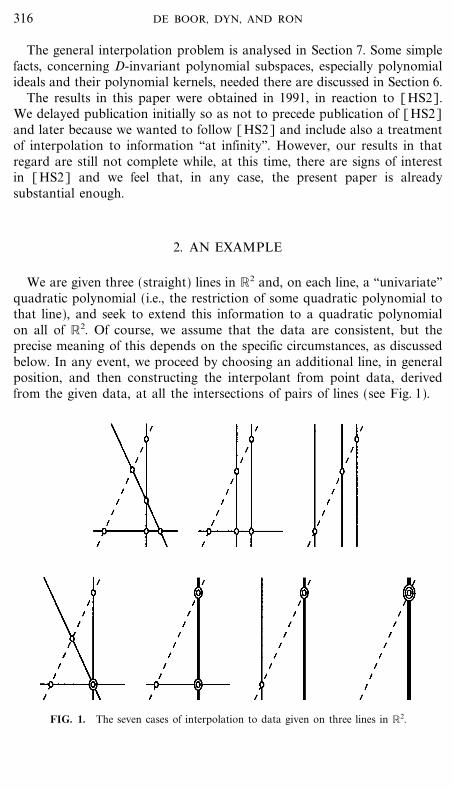
We are given three (straight) lines in R2 and, on each line, a `ùnivariate''quadratic polynomial (i.e., the restriction of some quadratic polynomial tothat line), and seek to extend this information to a quadratic polynomialon all of R2. Of course, we assume that the data are consistent, but theprecise meaning of this depends on the specific circumstances, as discussedbelow. In any event, we proceed by choosing an additional line, in generalposition, and then constructing the interpolant from point data, derivedfrom the given data, at all the intersections of pairs of lines (see Fig. 1).

FIG. 1. The seven cases of interpolation to data given on three lines in R2.


Case 1.1 (General Position). The three given lines are in generalposition, meaning that any two have exactly one point in common, andthis point does not lie on the third line.

In this case, a fourth line in general position will intersect each of thegiven lines at a point not also on another line, thus giving us a 6-point setthat is well known (see, e.g., [DR]) to permit unique interpolation fromthe space 62 of bivariate quadratic polynomials to arbitrary data. In par-ticular, let p be the interpolant from 62 to the data derived from the givenquadratic polynomials. This requires consistency, in the sense that, at thepoint common to two given lines, the corresponding polynomialsprescribed on these two lines have to agree. Then, on each of the givenlines, p reduces to a `ùnivariate'' quadratic polynomial. That quadraticpolynomial agrees with the original `ùnivariate'' quadratic polynomialgiven on the line, since they agree at three points on that line.

Case 1.2 (Two (But Not Three) Lines Are Parallel (But Not Coincident)).This is a limiting case of the Case 1.1, reached by rotating one of the lines.

Now our procedure produces only 5 points of intersection, hence inter-polation from 62 would be underdetermined. In this situation, [HS2]derive, in effect, information at the point at infinity at which the twoparallel lines intersect. We prefer to interpolate instead from a certain5-dimensional linear subspace P(5) of 62 . Precisely, 5=[!1 , ..., !4] is amatrix whose j th column contains a (nontrivial) vector perpendicular tothe j th line, j=1, ..., 4, and P(5) is the linear span of all functions of theform x [ > j # J (!j } x), with J such that [!i : i � J] spans R2.

In Case 1.1, P(5)=62 . In the present case, however, all elements ofP(5) are necessarily linear in the direction of the parallel lines (whichimplies that P(5) is obtained from 62 by the imposition of one linear con-straint). There is a unique interpolant from P(5) to the derived data at thefive points, provided that the data are compatible with P(5), i.e., providedthe polynomials given on the two parallel lines are actually linear (this isa special case of the general result in [DR], to be used in the sequel). Withthis proviso, the restriction of the interpolating polynomial to a given lineagrees with the given polynomial there since it matches it there at as manypoints as are needed, given the degrees involved, to conclude agreement onthe entire line from agreement at those points.

Case 1.3 (Three Parallel Lines). In this case, P(5) (defined as inCase 1.2) reduces to the 3-dimensional space of all quadratic polynomialsconstant in the direction of those three lines. Compatibility of the data nowmeans that they must be constant on each of those three lines, while con-sistency is vacuous here (since the lines have empty intersection). Withthat, existence of exactly one element of P(5) matching such data isevident.


The three cases covered so far are examples of what we call the simplecase; it leads to an interpolation problem of Lagrange type and the readeronly interested in this case may safely skip the rest of this section.

In the nonsimple, or general, case, one has to deal with interpolation toderivative information as well, derived from the given information (as inCase 2.1 below) and�or given explicitly (as in Cases 2.2�2.4 below).

Case 2.1 (The Three Lines Intersect at a Common Point, But No TwoLines Coincide). This is a limiting case of Case 1.1, reached by translating(but not rotating) one of the lines. In particular, P(5) does not change, i.e.,it is still 62 for this case. Having the function specified on a straight linemeans, of course, that we have also specified, on that line, any derivativeof any order in the direction of that line. Since, on R2, it takes just twodirectional derivatives at a point (in nonparallel directions) to specify everydirectional derivative at that point, consistency now requires that the threedirectional derivatives specified by the data at the point common to allthree lines be consistent. That being understood, the rest is as before, withthe slight complication that the common point is a triple point for inter-polation from 62 , and is a double point when arguing that the interpolantfrom 62 agrees with the given data on each of the three given lines.

Case 2.2 (Two Lines Are Coincident, the Third Not Parallel ). This is alimiting case of Case 1.2, as we translate (but not rotate) the given linessuitably, hence P(5) is the same as in Case 1.2. (It is also a limiting caseof Case 2.1, as we rotate one of the lines suitably.)

We now assume given on the double line also the derivative normal tothat line (necessarily a linear polynomial along that line even if we onlyknew that it was the normal derivative of some element of 62), hence knowon that line any directional derivative. The only change from the precedingcase is that some points now become double points and that we must (andcan) also verify that the given normal derivative is matched on the entiredouble line.

Case 2.3 (Three Parallel Lines, Two Coincident). This is a limiting caseof Case 1.3, as we translate (but not rotate) one of the given lines suitably,hence P(5) is the same as in Case 1.3. (It is also a limiting case of Case 2.2,as we rotate one of the lines suitably.)

We now assume given on the double line also the derivative normal tothat line, and compatibility requires (as in Case 1.3) that all data, includingthis normal derivative, be constant, making it easy to verify the existenceof exactly one element in P(5) that matches the given data.

Case 2.4 (Three Coincident Lines). This is a limiting case of Case 1.3(and Case 2.3) as we translate (but not rotate) the given lines suitably,


hence P(5) is the same as in Cases 1.3 and 2.3. (It is also a limiting caseof Case 2.2, as we rotate one of the lines suitably.)

In this case, assuming the data compatible with this, i.e., constant alongthe triple line, we also assume that the first and the second normalderivative is prescribed at that triple line (as a constant along that line) andconclude directly that the unique interpolant from P(5) matching theinformation at the triple point (picked out by our additional line) matchesthe given information on the entire triple line.

In this example, the orthogonal complement of a flat is only one-dimen-sional. The problem of choosing a minimal set of derivative information tobe specified on a repeated flat becomes significantly more complicatedwhen data are given on certain s-dimensional flats in Rd for s<d&1.

3. THE BASIC IDEA

Let H be a sequence of hyperplanes in Rd, let 0�s<d, and recall fromthe Introduction the collection Ms(H) of all s-dimensional intersections ofhyperplanes from H. We are interested in polynomial interpolation to datagiven at all the flats in Ms(H).

For s=0, this is the interpolation problem addressed in [DR]. Wepropose to reduce the general case s�0 to the known case s=0 by work-ing with the larger sequence Hs , obtained from H by adjoining to it shyperplanes in general position with respect to it, and then consideringinterpolation at all the points in M0(Hs) to data there as derived from thedata given on the flats in Ms(H). In this, we assume that the given data areconsistent, i.e., provide unambiguous information at the points in M0(Hs).Since [DR] readily provides a suitable interpolant to data on M0(Hs), thisreduces our task to showing that this interpolant does, indeed, match thedata given on the flats in Ms(H).

If the hyperplanes in H are in general position, then M0(Hs) consists ofexactly ( *Hs

d ) points, i.e., the cardinality of M0(Hs) equals the dimension ofthe space

6k

of all polynomials of degree �k, with

k :=*Hs&d=*H&(d&s).

More than that, in this case, 6k is well known to contain a unique inter-polant to arbitrary data given at the points in M0(Hs). In particular, let pbe that interpolant from 6k to data at M0(Hs) derived from the given data.


Then, assuming that the data are compatible, i.e., that the given datum pM

at a flat M in Ms(H) is the restriction to that flat of some element of 6k ,our interpolant p from 6k is guaranteed to agree with pM at sufficientlymany points to force its restriction to M to coincide with pM .

In the contrary case, various complications arise that will be dealt withfully later on. In the remainder of this introductory section, we now discussjust one such complication, namely the possibility that M0(Hs) consists offewer than dim 6k points but still each such point lies in exactly d of thehyperplanes from Hs . The latter condition characterizes what we call inthis paper the simple case. Already this case will provide the reader with agood feeling for the nature of the interpolation problem considered andsome of the difficulties overcome by us in solving it.

When *M0(Hs)<dim 6k , we can only interpolate at M0(Hs) fromsome subspace of 6k . Of the infinitely many choices possible, we take thesubspace used in [DR], as this permits us to prove (later on) existence anduniqueness of an interpolant from that space to arbitrary (consistent andcompatible) data given on Ms(H). For a description of that subspace, wefind it more convenient to switch now, from the hyperplanes, to theirnormals and associated constants.

Precisely, we think, as we may, of H as having been obtained from amatrix X, with d rows and no null column, and a corresponding scalarsequence (*x : x # X ) as the collection of hyperplanes

Hx :=[t # Rd : qx(t)=0]

with

qx : t [ x } t&*x ,

and with x running over the columns of the matrix X. The relation U/Xwe take to mean that U is obtained from X by deletion of some (or none)of its columns. Also, we denote by *X the length of the sequence X, i.e.,the number of columns of the matrix X. The ordering of the columns of Xis immaterial here. Because of the role such matrices play in box splinetheory, we call them direction sets (in Rd).

With this, we associate with each U/X the following homogeneouspolynomial of degree *U,

lU : t [ ù # U

(u } t), (3.1)

but write lx instead of l[x] or l[x] for x # X. Further, we introduce thefollowing subset of 2X,

L(X ) :=[L/X : rank(X"L)=rank X]. (3.2)


In these terms, [DR] show that (under the assumption that we are in thesimple case with s=0) there is a unique interpolant to arbitrary values onthe set M0(H) from the polynomial space

P(X ) :=span[lL : L # L(X )]. (3.3)

Note that P(X )=6*X&d in case H is in general position (provided thatthere are at least d hyperplanes in the sequence). For more information onP(X ), see Section 4 below.

Now let Y be a sequence of s directions, or, equivalently, a (d_s)-matrixof directions associated with the s hyperplanes in general position adjoinedto H to obtain Hs , and continue to assume that we are in the simple case,i.e., each point in M0(Hs) lies in exactly d of the hyperplanes in Hs . Set

Z :=X _ Y.

Then [DR] provides a unique interpolant from P(Z) to arbitrary valuesat the points of M0(Hs). We will show below that

P(Z)=Ps(X ) :=P(X ) 6r :=span[ pq : p # P(X ), q # 6r],

with r :=(s&d+rank(X ))+ . In particular, P(Z) only depends on X and s.Assume now that we have been given consistent data on the flats in

Ms(H), i.e., data

( pM : M # Ms(H))

so that, for every M1 , M2 # Ms(H), the polynomials pM1and pM2

coincideon M1 & M2 & M0(Hs). Such consistency is clearly necessary if we are toconstruct an interpolant to these data.

For each % # M0(Hs), there exists some basis B/Z such that % # Hx forevery x # B. Since *Y=s, X & B contains some B$ of length d&s. There-fore, M :=�x # B$ Hx is a flat in Ms(X ) that contains %, hence the deriveddatum

a% :=pM(%)

is well-defined. Also, by the assumed consistency, this definition isindependent of our choice of M.

It follows from [DR, Theorem 7.1] (see Theorem 5.11 below) that thereis exactly one element of P(Z) that matches these data (a% : % # M0(Hs)).To show that, for all M # Ms(H), this element also matches pM on M takesadditional work; see the proof of Theorem 5.10 below. In particular, forsuch a conclusion, we need to assume that the given data are X-compatiblein the sense that each pM is the restriction to M of some element of P(Z).


But the above discussion already makes clear that an interpolant fromP(Z) to any X-compatible and consistent data on Ms(H) is unique.

4. THE SPACE Ps(X )

In this preparatory section, we discuss the polynomial space Ps(X ), to beused eventually as the space of interpolants to information given on certainflats determined by X.

We start off with a direction set, as introduced in the preceding section,i.e., a matrix X with d rows and no null columns. We denote the columnspan of X by

ran X.

Recall from (3.3) the polynomial space

P(X ) :=span[lL : L # L(X )] (4.1)

with

lU : t [ `x # U

(x } t), (4.2)

and

L(X ) :=[L/X : rank(X"L)=rank X]. (4.3)

This polynomial space naturally arises in box spline problems. It reflects inits structure much of the geometry of the multiset X, and was independ-ently discovered by several authors ([HS1, J, DR]; some of us regret thatthis is the chronological order; see also [DM]).

Now note that lL is a homogeneous polynomial of (exact) degree *L,and is constant in all directions perpendicular to ran L, i.e., DzlL=0 for allz = ran L. Since each L # L(X ) can have at most *X&rank X elements, itis clear that P(X ) is a dilation-invariant subspace of 6*X&rank X (ran X ),with

6k(M)�6

the subspace of all polynomials of degree �k on Rd that are constant inall directions orthogonal to the flat M. It is also clear that P(X )=P(X _ B), with B any basis for a linear subspace complementary to ran Xsince L(X )=L(X _ B) for any such B. The dimension of P(X ) is known toequal the number of submatrices of X that are bases for ran X. For more


information, see, e.g., [DR]. It is important to note that if X is in generalposition (i.e., if every U/X with *U�rank X is 1-1), then the space P(X )coincides with 6*X&rank X (ran X ).

We are ready for the definition of Ps(X ).

Definition 4.4. Let X be a direction set and let s be an integer. Then

Ps(X ) :=P(X ) 6 (s&d+rank(X ))+. (4.5)

Note that Ps(X )=P(X ) for s�d&rank(X ), and that the sequence(Ps(X ) : s=0, 1, 2, ...) is nested, i.e., Ps$(X )�Ps(X ) whenever s$<s.

In the sequel, the following characterization of Ps(X ) will be importantsince it shows the characterization of P(5) from [DR] to be applicablehere, and shows that, for Y in general position, P(X _ Y ) only depends onX and *Y:

Proposition 4.6. Let X and Y be direction sets in Rd, with X _ Y of fullrank, and s :=*Y. Then

P(X _ Y )�Ps(X ),

with equality if (and only if ) Y is in general position with respect to X, i.e.,no y # Y lies in a proper subspace spanned by elements of (X _ Y )"y.

Proof. Since X _ Y is of full rank by assumption, Y must contain somebasis B for a subspace complementary to ran X. Then X _ B is of fullrank, P(X _ B)=P(X ) and s&d+rank(X )=*(Y"B). We may thereforeassume without loss that already X is of full rank, hence

Ps(X )=P(X ) 6s .

Given L # L(X _ Y ), we let k :=*(L & Y ). Then the rank-d matrix(X _ Y )"L contains exactly s&k elements from Y, and thus rank(X"L)�d&(s&k). Since rank X=d, there exists Z/L & X with *Z�s&k suchthat rank((X"L) _ Z)=d. Now,

lL=lL"(Y _ Z)l(L & Y ) _ Z , (4.7)

and we have that *((L & Y ) _ Z)�k+(s&k)=s, hence l(L & Y ) _ Z # 6s .At the same time, L"(Y _ Z) is a subset of X, and its complement in X is(X"L) _ Z which is known to be of full rank. This means that L"(Y _ Z) #L(X ), and therefore lL"(Y _ Z) # P(X ). Consequently, we infer from (4.7)that lL # P(X ) 6s . This being true for every L # L(X _ Y ), we concludethat a spanning set for P(X _ Y ) lies in Ps(X ), and henceP(X _ Y )/Ps(X ).


For the converse inclusion, let L # L(X ), and let B/(X"L) be a basis forRd (i.e., a square invertible d_d matrix) The existence of such a B isguaranteed by the definition of L(X ) and our assumption that rank X=d.Let Z :=B _ Y. Then *Z=s+d, and, by our assumption on Y, Z is ingeneral position, hence P(Z)=6s . This implies that, given an element ofthe form lLq with q # 6s , we are able to write this polynomial in the form

lLq= :L$ # L(B _ Y )

cL$lL _ L$

for certain scalars cL$ . Each L _ L$ in this sum lies in L(X _ Y ) since(X _ Y )"(L _ L$)#(B _ Y )"L$, and the latter is of rank d becauseL$ # L(B _ Y ). Consequently, lLq # P(X _ Y ), and we have thus provedthat a spanning set for Ps(X ) lies in P(X _ Y ), and hence Ps(X )/P(X _ Y ).

Finally, the `ònly if '' assertion follows from the above proof and theknown formula for the dimension of P(X ) as follows. Suppose that Y is notin general position with respect to X, and let Z be a set of s directions thatis in general position with respect to X. Then, X _ Z contains more basesthan does X _ Y. Since this basis count determines the dimension of thecorresponding P-space, it follows that dim P(X _ Y )<dim P(X _ Z).However, we proved above that P(X _ Z)=Ps(X ), whence the desiredconclusion. K

5. THE INTERPOLATION PROBLEM: THE SIMPLE CASE

Recall that we introduced the direction set X as a sequence or matrix ofnormal vectors, one for each of the hyperplanes

Hx :=[t # Rd : x } t=*x], x # X,

in the given sequence H, with suitable constants *x # R. These constantswill be held fixed throughout the discussion. With s # [d&rank(X ), ..., d&1]fixed, we wish to interpolate to polynomial information given on thecollection

Ms(X ) :={ ,x # U

Hx : U/X, rank U=d&s= (5.1)

of all flats of dimension s that can be expressed as the intersection of hyper-planes from (Hx : x # X ). Note that we have now switched, from thenotation Ms(H) to the (less precise) notation Ms(X ). Since the hyperplanes(Hx : x # X ) depend on (*x : x # X ), so does the set Ms(X ), but we have


suppressed the * subscript here, as we did with Hx , since these constantsare being held fixed throughout. However, we will write

Ms, 0(X )

instead of Ms(X ) when we want to stress the fact that all hyperplanescontain the origin, i.e., in the determination of these s-dimensional flats, all*x were chosen to be zero.

For each M # Ms(X ), we consider the following subset X M of X,

XM :=(x # X : M/Hx). (5.2)

By the definition of Ms(X ), rank XM=d&s, and thus *XM�d&s.

Definition 5.3. Let X, *=(*x : x # X ), and Ms(X ) be as above. Wecall the pair (X, *) simple if each M # Md&rank X (X ) is contained in no morethan rank X hyperplanes from H, i.e., if *XM=rank X for each such M.In that case, we also call the corresponding interpolation problem simple.

For instance, in the example in Section 2, the Cases 1.1�1.3 are simple,while the Cases 2.1�2.4 are not. Note that Md&ran X (X ) is just the pointsetM0(X ) in case X is of full rank and has at least d columns. In other words,if rank X=d, then simplicity means that each % # M0(X ) is the intersectionof exactly d hyperplanes in H.

For the rest of this section, we assume that our interpolation problem issimple. Note that this assumption is entirely on the constants (*x : x # X )and not on the matrix X.

We now assume that, with each flat M # Ms(X ), we are given a polynomialpM on M, i.e., the restriction p|M of some p # 6, and it is this polynomialinformation we hope to match by some element of Ps(X ). We will not beable to accomplish this unless

pM # Ps(X )|M . (5.4)

Surprisingly, this simple necessary condition for the existence of a solutionto our problem (along with the obvious consistency condition discussedbelow) is also sufficient, leading to the following.

Definition 5.5. The data ( pM : M # Ms(X )) are termed X-compatible if(5.4) holds for every M # Ms(X ).

We now take time out to study this notion of compatibility in some depth.The analysis of our interpolation problem is resumed after Proposition 5.8.


In order to characterize X-compatible data and for later use, we nextprove that, on M, Ps(X ) coincides with P(ZM) for a certain direction setZM . The construction of ZM involves the orthogonal projector

PM

onto the linear subspace M&M parallel to the flat M. Explicitly,

ZM :=PM(Z"ZM) _ BM ,

with

Z :=X _ Y, (5.6)

with Y an arbitrary s-set of directions in general position with respect toX, and with BM any basis from ZM for the orthogonal complement

M= :=[t # Rd : t = (M&M)]

of M in Rd. Having made appropriate choices for Y and BM , we now keepthem fixed for the remainder. Note that, necessarily, P(ZM)/6(M). Theexclusion of ZM is needed since PM maps all of ZM to 0. Here is therelevant formal statement and its proof.

Lemma 5.7. Let Z be a direction set, and let M # Ms(Z). Then

P(Z)|M=P(ZM)| M .

In particular, with Y an s-direction set in general position with respect to X,

Ps(X )| M=P((X _ Y )M)|M , \M # Ms(X ).

Proof. The map

L [ L� :=PM(L"ZM)

carries L(Z) onto L(ZM). Indeed, PM carries a spanning set of Rd to a span-ning set of M&M, hence PM(Z)"L� =PM(Z"L) spans M&M. ThenPM(Z"ZM)"L� spans M&M, too, since it differs from PM(Z"L) byPM(ZM)=[0]. Since ZM "L� =PM(Z"L) _ BM , and since BM spans M =,we conclude that L� # L(ZM).

To show that the map is onto, let K # L(ZM). Since ZM contains exactlyd&s elements (viz., the elements of BM) not contained in the s-dimensionalM&M, and since ZM"K spans Rd, K must be disjoint from BM . Hence Klies in PM(Z"ZM). In particular, K=PM(L) for some L/Z"ZM. On theother hand, ZM "K spans Rd, and is the union of BM and PM(Z"ZM)"K.Therefore, since rank(BM)=d&s, we have that rank(PM(Z"ZM)"K)�s,


a fortiori rank(Z"(ZM _ L))�s. It easily follows then that rank(Z"L)=d,hence that L # L(Z).

With this, let L # L(Z) and consider lL on M. If t # M, then

lL(t)= `x # L

(x } t)= `x # L

((PMx) } t+(x&PMx) } t),

and cx :=(x&PMx) } t is a constant on M. This shows that, on M, lL

agrees with some scalar multiple of the function f: t [ >x~ # L� (x~ } t+cx),and, since L� # L(ZM), such f is in P(ZM) (as a linear combination of poly-nomials of the form lK , K # L(X )). Consequently, P(Z)|M �P(ZM)|M . Theconverse containment is obtained in an analogous way.

The second equality in the lemma is a consequence of the first and ofProposition 4.6. K

We recall from [BDR, (2.22)] that, for a full-rank direction set 5, p # 6is in P(5) iff, for every 1�r�d and every N # Mr, 0(5) and every t # Rd,

deg ( p| t+N)�*(5"N=)&r.

After identifying the datum pM given on M # Ms(X ) with its unique exten-sion to an element of 6(M)/6, we therefore obtain, with the aid ofLemma 5.7, the following.

Proposition 5.8. The data ( pM : M # Ms(X )) are X-compatible if andonly if, for r�s and every N # Mr, 0(ZM) and every t # M&M,

deg ( pM | t+N)�*(ZM"N=)&r=*(XM "N=)+s&r.

We now resume the discussion of our interpolation problem. We want tointerpolate all the data ( pM : M # Ms(X )) by some p # Ps(X ), hence mustensure also that these data are consistent enough to guarantee the existenceof a smooth interpolant at least locally. These conditions, which we referto as ``the consistency conditions'', are very natural and simple in thepresent case.

Definition 5.9. We say that the data ( pM : M # Ms(X )) are consistentif, for every M1 , M2 # Ms(X ), the polynomials pM1

and pM2coincide on

M1 & M2 & M0(Z) (with Z as in (5.6)).

Theorem 5.10. Assume that (X, *) is simple, and let ( pM : M # Ms(X ))be consistent and X-compatible data. Then there exists exactly one p # Ps(X )that interpolates these data, i.e., that satisfies

p|M= pM , \M # Ms(X ).


If s=0, then the information is given at points. In this case,Ps(X )=P(X ), and both the consistency and compatibility conditions arevacuous. Thus, for the case s=0, our theorem reads as follows:

Theorem 5.11 [DR]. Any data given on the pointset M0(X ) isinterpolated by a unique element in P(X ).

The existence part of this theorem can be easily proved by finding inP(X ) Lagrange polynomials for the data, i.e., polynomials that vanish atall points in M0(X ) but one. The uniqueness is harder and can be provedby showing that dim P(X )=*M0(X ). We omit all these details sinceTheorem 5.11 has already been proved in [DR]; it is a special case ofTheorem 7.1 there, which covers also the general case for s=0, Theorem 7.4,here. The construction of the Lagrange polynomials together with the factthat these polynomials form a basis for P(X ) is the content of Theorem 4.1of [DR].

We now reduce the general Theorem 5.10 to the known Theorem 5.11:

Proof of Theorem 5.10. Recall the direction set Y # Rd_s in generalposition with respect to X chosen earlier and the notation Z :=X _ Y, andthe fact that, by Proposition 4.6, Ps(X )=P(Z). We associate with eachy # Y a constant *y such that also M0(Z) is simple, i.e., such that exactlyd hyperplanes Hz , z # Z, contain a given point % # M0(Z). Our proof thenproceeds in two steps: the first one, we already took in Section 3, where weused the assumed consistency to show that the given information( pM : M # Ms(X )) determines uniquely data values (a% : % # M0(Z)), andthen invoked Theorem 5.11 to find exactly one p # P(Z)=Ps(X ) that inter-polates these data, thus concluding uniqueness of the interpolant. In thesecond step, we show that, for every M # Ms(X ), the fact that the inter-polant p coincides with pM on M & M0(Z) implies that p= pM on all of M,thus showing existence of the interpolant.

Here are the details for that second step.To prove the existence, we fix M # Ms(X ) and wish to show that the

interpolant p coincides on M with pM . Now, pM and p|M agree onM0(Z) & M, and both are in P(Z)|M (the former by the assumed X-com-patibility and the latter by construction), while P(Z)|M=P(ZM)| M , byLemma 5.7. Further, by Theorem 5.11 (easily applied to the current situa-tion by an affine change of variables), the space P(ZM) contains a uniqueinterpolant to arbitrary data at the point set M� (ZM), with the tilde indicat-ing that the zero-dimensional flats are constructed from hyperplanesHx~ =[t : qx~ (t)=0], x~ # ZM , and the corresponding constant *x~ in thelinear polynomial qx~ : t [ x~ } t&*x~ chosen in such a way that qx~ agrees onM with the polynomial qx , as is done in the proof of Lemma 5.7. Thus, we


can conclude that p|M= pM (and so declare Theorem 5.10 proved), oncewe prove that

M0(Z) & M=M� 0(ZM). (5.12)

For this, % # M� 0(ZM) iff the submatrix Z%M of all directions x~ # ZM with

% # Hx~ contains a basis for Rd. Any basis in ZM necessarily contains thebasis BM for M=, hence M� 0(ZM)/M. For any other element x~ of such abasis, we have Hx~ & M=Hx & M, by the construction of Hx~ just detailed,hence % also lies in the corresponding Hx . Consequently, M0(Z) & M#

M� 0(ZM).Conversely, % # M0(Z) & M iff the submatrix Z% of all directions x # Z

with % # Hx contains some basis B for Rd and, within that basis, a basis forM= taken from XM. For any element x # B"X M, qx=qx~ on M, hence% # M� 0(ZM). This finishes the proof of (5.12) and, thereby, the proof of thetheorem. K

6. SOME FACTS ABOUT POLYNOMIALS

Some of the theorems (in the next section) that are needed for provingour main result make claims of the form

F/G, (6.1)

with both F and G a polynomial space (i.e., a linear subspace of 6), but notnecessarily of finite dimension nor of finite codimension. However, in allcases of interest to us, the spaces F and G are D-invariant i.e., invariantunder differentiation in any direction, hence invariant under any constant-coefficient differential operator p(D) :=�: (D:p(0)�:!) D:, taken as a mapon 6, with D: :=>d

i=1 D:(i)i , and D i differentiation with respect to the ith

argument.For D-invariant F and G, one may try to prove the inclusion F/G by

inspecting the constant-coefficient differential operators that annihilatethese spaces, since, for an arbitrary subset G of 6, the set

IG :=[ p # 6 : G/ker p(D)]

is an ideal (hence has a finite generating set) and, further,

G/ker IG := ,p # IG

ker p(D)= ,p # G0

ker p(D)


for any generating set G0 for IG , with equality if and only if G is a co-ideal,i.e., a D-invariant polynomial space that is closed in the weak topologyinduced by the pairing

6_6: ( p, q) [ (p, q) :=::

D:p(0) D:q(0)�:!.

Hence, if G is a co-ideal, then we can conclude (6.1) as soon as we knowthat, for all p in some generating set for the ideal IG , p(D) annihilates F.For, then we know that IG /IF , hence

F/ker IF /ker IG=G.

In our particular applications, G will be a homogeneous polynomialspace, i.e., is spanned by homogeneous polynomials (or, equivalently, isinvariant under dilations). For that case, we have the following simple, yetvery useful, observation:

Proposition 6.2. Any sum of homogeneous D-invariant polynomialspaces is a co-ideal.

Proof. Since the sum of homogeneous D-invariant polynomial spaces isalso homogeneous and D-invariant, we need only to prove the case whenthere is a single summand, F, in the sum.

Since we assume that F is D-invariant, we need only to prove that it isclosed. Let ( fn) be a sequence in F weakly convergent to f # 6. Then f # 6k

for some k and so, necessarily, already

f [k]n =: :

|:|�k

D:fn(0):!

( ):

converges weakly to f, while, by the homogeneity of F, each f [k]n is in the

finite-dimensional space F & 6k , hence so must f be. K

We conclude this section with two further simple observations of use inthe next section.

Proposition 6.3. Let F and G be co-ideals, with IG=I(1), and letp # 6. Then, p # F+G if and only if there exists f # F so that, for all # # 1,#(D)( p& f )=0.

For our last statement, let M be a flat in Rd and recall our notation PM

for the orthogonal projector onto M&M. Then,

Dy p=DPMy p, \y # Rd, \p # 6(M). (6.4)


Indeed, since p # 6(M) is constant in all directions perpendicular to M, wehave Dy&PMy p=0.

In particular, Dy maps 6(M) onto itself unless PMy=0, i.e., unlessy # M=. Since Dy(qp)=(Dy q) p+q(Dyp), this implies (by induction ondeg q) the following

Proposition 6.5. For any flat M in Rd, any y # Rd"M=, and anyD-invariant linear subspace F of 6,

Dy(F6(M))=F6(M).

7. THE INTERPOLATION PROBLEM: THE GENERAL CASE

The basic set-up in the general case is the same as in the simple case: weare given the direction set X and the constants (*x : x # X ) and want tointerpolate from Ps(X ) to polynomial information given on the flats inMs(X ). Only that at this time, we no longer assume simplicity, i.e., whilestill for every M # Ms(X ) the set XM (of all vectors whose correspondinghyperplane contains M) spans M=, there might be more than d&s vectorsin XM, which is to say that the flat M appears with some multiplicity.Therefore, the initial task is to define precisely the multiplicity notion. Thiswill eventually determine the type of interpolation conditions we expect tosatisfy.

Before embarking on the precise definition of ``multiplicity'' here, wemake the following simple count: suppose that M # Ms(X ) is given andassume that XM contains more than d&s vectors. In this case, the inter-polating polynomial should match not only function values given on M butalso some prescribed derivatives on M, i.e., we expect to be given data

( pM, . : . # 8)

consisting of polynomials on M, with 8 some M-dependent polynomialspace that describes the derivatives to be interpolated, in the sense that werequire our interpolant p to satisfy all of the conditions

(.(D) p)|M= pM, . , \. # 8.

Of course, some consistency requirements must be enforced; for example,it should be assumed that

:pM, .+;pM, �= pM, :.+;� , \., � # 8, \:, ; # C.


As we will see in a moment, the exact definition of the space 8 is fairlycomplicated, but one thing can be observed easily in advance: the dimen-sion of 8 should be the number of bases for M= that can be extracted fromXM (i.e., the number of submatrices of XM of length and rank d&s). Thisis so because this number counts the number of flats in Ms(X ) that havebeen merged into the one M while passing from the generic or simple caseto the present general case.

We now define exactly the type of derivatives that should be inter-polated. For this purpose, we recall the polynomial space D(5) which isalso intimately related to box spline theory:

Definition 7.1. Let 5 be any matrix with d rows. Let K(5) be thecomplement of L(5) in 25, i.e.,

K(5) :=[K/5 : rank(5"K)<rank 5]. (7.2)

Then the polynomial space D(5)/6(ran 5) is defined as the joint kernelof the differential operators on 6(ran 5) induced by K(5):

D(5) :=[. # 6(ran 5) : lK (D) .=0, \K # K(5)]

=ker I(lK : K # K(5))/6(ran 5).

In particular,

D(5)=D(5 _ B)

for any basis B for (ran 5)=.

We are now ready to describe the information to be interpolated: weassume that the data consist of polynomials

pM, . # 6(M), M # Ms(X ), . # D(X M),

and that the interpolant p should then satisfy

(.(D) p)|M= pM, . , \M # Ms(X ), \. # D(X M).

It may be helpful for the reader to consider briefly the spaces D(XM)that occur in the example in Section 2. In Cases 1.1�1.3 and 2.1, each XM

has just one column, XM=[x] say, and, correspondingly, K(XM)=[[x]], hence D(XM)=60 . In Cases 2.2 and 2.3, one of the M has XM=[x, x] for a certain x, hence now K(XM)=[[x, x]], and thereforeD(XM)=61(ran[x])=span[1, lx]. Finally, Cases 2.4 is quite similar inthat the one and only M has XM=X=[x, x, x], hence D(X M)=span[1, lx , l2

x] in this case. As we said at the end of Section 2, one needs to go


to higher dimensions in order to fully appreciate the power of the constructD(XM).

We postpone the discussion concerning the consistency of the data, butwe can already present our compatibility requirements for the datawith Ps(X ):

Definition 7.3. We say that the given data ( pM, . : M # Ms(X ),. # D(XM)) are X-compatible if

pM, . # (Ps(X ))|M , \M # Ms(X ), \. # D(XM).

While one might have expected here the stronger condition pM, . #(.(D) Ps(X ))|M , the given condition turns out to suffice.

So, with the notion of consistency yet to be defined, we assume that weare given consistent information ( pM, . : M # Ms(X ), . # D(XM)) that isX-compatible and want to prove the existence and uniqueness of p # Ps(X )that matches these data. As in the simple case, our solution method isbased on the reduction of this problem to the case s=0 and uses theknown results for this case that were established in Theorem 7.1 of [DR],as follows.

Theorem 7.4 [DR]. Let 5 be a direction set in Rd, of rank d, and let(Hx : x # 5) be a corresponding sequence of hyperplanes, each perpendicularto its associated x. For each % # Rd, let 5% be defined as

5% :=(x # 5 : % # Hx),

and let M0(5) be the set of all % with rank 5 %=d. Then, for every smoothfunction f: Rd � C, there exists exactly one p # P(5) that satisfies

.(D) p(%)=.(D) f (%), \% # M0(5), \. # D(5 %).

The smooth function f in this theorem serves only to ensure theconsistency of the data (.(D) f (%) : % # M0(5), . # D(5 %)). We could havereplaced each value .(D) f (%) by a number p%, . and required theconsistency conditions

:p%, .+;p%, �= p%, :.+;� , % # M0(5), ., � # D(5%), :, ; # C,

since these conditions are equivalent to the existence of a smoothinterpolant to the data.

With the aid of Theorem 7.4, we treat the case s>0 as follows: Weassume that Ms(X ) is not empty (since otherwise there is nothing toprove), i.e., we assume that rank X�d&s, and add to X, as in the simple


case, s vectors Y that are in general position relative to X, thus obtainingthe direction set

Z :=X _ Y,

of full rank. Since, by Proposition 4.6, Ps(X )=P(Z), we seek ourinterpolant from P(Z). Precisely, we will derive from the data( pM, . : M # Ms(X ), . # D(XM)) uniquely determined data ( p%, . : % #M0(Z), . # D(Z %)) and show that the unique interpolant in P(Z) to thelatter data (which is provided by Theorem 7.4, with 5=Z) also interpolatesthe original data.

Our first step is to derive the information ( p%, � : % # M0(Z), � # DD(Z %))from the given data ( pM, . : M # Ms(X ), . # D(X M)). Precisely, we think ofeach pM, . as specifying (.(D) p)|M , with p being our desired interpolant,and want to be able to compute from this information the numbers�(D) p(%) for � # D(Z%) and % # M0(Z).

We fix now % # M0(Z) and proceed as follows: we first remove fromMs(X ) all flats that do not contain %. The remaining set is easily shown tocoincide with Ms(X %), i.e., the set of s-dimensional flats associated with thehyperplanes that contain %. The information available to us at % is of theform

( pM, .(%) : M # Ms(X%), . # D(X M)).

However, since pM, . specifies .(D) p on all of M, we thereby also knowq(D) .(D) p on M for any q # 6(M). This means that the data supply thenumber .(D) p(%) for any

. := :M # Ms (X %)

:i

.Mi qM

i # :M # Ms (X%)

D(XM) 6(M),

in the form

.(D) p(%)= :M # Ms (X %)

:i

qMi (D) pM, .i

M (%).

Of course, for this to work, we must be certain that the resulting number.(D) p(%) is independent of the particular way we are writing . as such asum. This leads to the following.

Definition 7.5. We say that the given data ( pM, . : M # Ms(X ),. # D(XM)) are consistent if, for some Y # Rd_s in general position withrespect to X and for every % # M0(Z) (with Z :=X _ Y ),

0= :M # Ms (X %)

:i

.Mi qM

i # :M # Ms (X %)

D(XM) 6(M)


implies that

:M # Ms (X %)

:i

qMi (D) pM, .i

M (%)=0.

Note that such consistency is demanded here only at certain finitelymany points, which is very helpful, since an equivalent definition on anentire intersection of flats seems to be comparatively awkward.

It follows that the original information determines the desired informa-tion (�(D) p(%) : � # D(Z%)) if and only if

D(Z %)/ :M # Ms (X%)

D(XM) 6(M). (7.6)

As we now explain, it suffices to establish the above inclusion for thespecial case when X %=X, and %=0; Theorem 7.7 below establishes theinclusion for this seemingly special case. The general case of (7.6) thenfollows by the following reasoning.

First, since Z% & X=X %, and since each XM (with M # Ms(X%)) is a sub-matrix of X% (and not only of X ), the vectors in X"X% play no role here,hence nothing is lost in assuming X%=X. Second, assuming X%=X, themap

M [ M&%

maps Ms(X ) 1-1 onto Ms, 0(X ). At the same time, since all the spacesinvolved in (7.6) are translation-invariant, nothing is changed there if wetranslate them all by %; the only change is that the index set Ms(X )=Ms(X %) of the summation is replaced by Ms, 0(X ).

Consequently, (7.6) will be proved as soon as we have shown the following:

Theorem 7.7. Let 5 be a direction set in Rd. Let s # [1, ..., d&1], andlet Y be an arbitrary collection of k�s vectors. Then

D(5 _ Y )/ :M # Ms, 0(5)

D(5 & M=) 6(M). (7.8)

We note that the statement in the theorem is sharp: for example, if 5 _ Yis in general position and Y contains exactly s vectors, then the inclusionof (7.8) already ceases to hold if we remove from the right-hand side anysingle summand. For, in that case, each D(5 & M=) equals 60 , while, forany M # Ms, 0(5), p :=l5"M= is of exact degree *5+s&d, hence p(D) failsto annihilate D(5 _ Y )=6*5+s&d , yet it annihilates all the summands inthe right-hand side except 6(M).


On the other hand, the two sides in (7.8) are never equal since the leftside is contained in 6*5+s&d while the right side contains polynomials ofarbitrarily high degree.

In order to prove the theorem, we observe that both sides of (7.8) are co-ideals, the right side by Proposition 6.2. The claim of the theorem followsthen from the fact (about to be established) that the ideal that determinesthe right-hand side of (7.8) is contained in the ideal that determines theleft-hand side.

As a matter of fact, D(5 _ Y ) is defined as the kernel of the ideal

I(lK : K # K(5 _ Y )).

Since the space D(5 _ Y ) gets larger with increasing Y, we will assumewithout loss that *Y=s. On the other hand, the following theorem assertsthat the right-hand side of (7.8) is the kernel of the ideal I(lK : K/5,rank(5"K)<d&s). Since Y has only s elements, each such K is inK(5 _ Y ). Thus, the next theorem provides a proof for (7.8).

Theorem 7.9. Let 5 be a direction set in Rd, let s be a non-negativeinteger �d, and let

Ks(5)

be the collection of all K/5 that are minimal with respect to the propertythat rank(5"K)<d&s. Then

:M # Ms, 0(5)

D(5 & M =) 6(M)= ,K # Ks (5)

ker lK (D)=: Ds(5). (7.10)

Proof. We note that, necessarily, rank(5"K)=d&s&1 for all K # Ks(5),and that K0(5) consists of all minimal elements of K(5), hence

D(5)=ker I(lK : K # K0(5))=D0(5).

Also, both sides of (7.10) are co-ideals (the left side by Proposition 6.2),hence their equality is equivalent to the equality of their correspondingideals.

As a warm-up, we prove the simpler inclusion in (7.10) by showing thateach of the operators lK (D) in (7.10) annihilates the left-hand side of(7.10). Indeed, if K # Ks(5) and M # Ms, 0(5), then 5"K has rank<d&s=rank 5 & M=, therefore (5 & M=)"(K & M=) has rank<rank(5 & M=),i.e., K & M= # K(5 & M=). But since, for every q # 6(M) and anyx # 5 & M=, lx(D)( pq)=(lx(D) p) q, this shows that lK & M=(D) annihilatesevery pq with p # D(5 & M=) and q # 6(M), hence annihilates all ofD(5 & M=) 6(M); a fortiori, that latter space is annihilated by lK (D).


We now prove the converse. First, if rank 5<d&s, then Ms, 0(5)=[ ]and also Ks(5)=[ ], hence both sides of (7.10) are [0]. We settle thecontrary case by induction on *5�d&s. If *5=d&s, then Ds(5)=�x # 5 ker Dx , and hence indeed Ds(5)=60(M), with M :=5 = the singleelement of Ms, 0(5).

Assume now that the statement of the theorem holds for 5, and let

Z :=5 _ [ y].

Assume that .(D) annihilates �M # Ms, 0(Z) D(Z & M=) 6(M). Since thissum contains the left-hand side of (7.10), the induction hypothesis impliesthat . # I(lK : K # Ks(5)), i.e.,

.=: :K # Ks (5)

lK �K ,

where (�K) are some polynomials. We need to show that . # I(lU : U #Ks(Z)). We do this by showing that

lK0�K0

# I(lU : U # Ks(Z))

for every K0 # Ks(5).Here is the way the proof goes. If K0 # Ks(Z), there is nothing to prove.

Otherwise, (5"K0) _ [ y] is of rank d&s. Let M # Ms, 0(Z) be the subspaceperpendicular to (5"K0) _ [ y]. We will show below that �K0

(D)annihilates D((5"K0) _ [ y]) 6(M), hence (see the proof of Proposition 6.2)�K0

# I(lK : K # K((5"K0) _ [ y])).The desired result follows from this since, for any K # K((5"K0) _ [ y]),

Z"(K0 _ K)=((5"K0) _ [ y])"K, with the latter matrix of rank<d&s,therefore some submatrix of K0 _ K lies in Ks(Z). Hence, lK0

�K0lies in the

ideal generated by [lU : U # Ks(Z)] which is exactly what we had to prove.It remains to prove that �K0

(D) annihilates D((5"K0) _ [ y]) 6(M). Forthis, we observe that

Z & M=#(5"K0) _ [ y]=(Z & M =)"K0 .

By assumption, �K # Ks (5) lK (D) �K (D) annihilates D(Z & M=) 6(M). Inaddition, there are certain terms in this sum that already annihilateD(Z & M=) 6(M) (without any `àid'' from other terms): if K # Ks(5), thenrank(5"K)=d&s&1, hence (5"K)/3 M= implies that rank((5"K) & M=)<d&s&1. Therefore, for such K, ((5"K) _ [ y]) & M= is of rank<d&sand, since this last matrix is (Z & M=)"K, we conclude that K & M= #K(Z & M=) which means that lK & M=(D) annihilates D(Z & M =) and henceannihilates D(Z & M=) 6(M). Thus, for such K, the operator lK (D) �K (D)


annihilates D(Z & M=) 6(M), and consequently, the sum of the rest of thesummands annihilates this space as well.

Thus, with

KMs :=[K # Ks(5) : (5"K)/M=],

we know that

:K # Ks

M(lK�K)(D)

annihilates D(Z & M=) 6(M). We also know that our original K0 is inKM

s . Also, (Z & M=)"(K0 & M =)=(Z & M =)"K0=(5"K0) _ [ y]. Thismakes the following map interesting for us.

Identifying M= with Rd&s, we define

L: D(Z & M=) � XK # Ks

MD((Z & M=)"(K & M=)) :

p [ (lK & M=(D) p : K # KMs ).

Note that by varying K over KMs , we actually vary K & M= over all mini-

mal submatrices of 5 & M= whose complement in 5 & M= does not spanM= any more. I.e., [K & M= : K # KM

s ]=K0(5 & M=). Thus, by [DM,Theorem 3.2] (a complete proof of which can be found, e.g., in [BRS]),the map L is onto, and therefore, for our K0 there exists F/D(Z & M =)such that lK & M =(D) F=0 for K # KM

s "[K0] but lK0 & M=(D) F=D((Z & M=)"K0). Thus, for K # KM

s "[K0],

lK (D) �K (D)(F6(M))=lK"M=(D) �K (D)((lK & M =(D) F ) 6(M))=[0],

and so,

[0]=: lK (D) �K (D)(D(Z & M =) 6(M))$: lK (D) �K (D)(F6(M))

=lK0(D) �K0

(D)(F6(M))=lK0"M =(D) �K0(D)((lK0 & M=(D) F ) 6(M))

=�K0(D)(lK0"M =(D)(D((Z & M=)"K0) 6(M)))

=�K0(D)(D((Z & M=)"K0) 6(M)),

the last equality since, by Proposition 6.5, lY (D) is a surjectiveendomorphism on every space of the form F6(M), with F a D-invariantpolynomial space, provided that Y & M==[ ]. Noting that (Z & M =)"K0

is exactly our old (5"K0) _ [ y], we have proved what we wanted to. K


Now, we finally know that the information required for solving the inter-polation problem related to M0(X _ Y ) is uniquely determined by theoriginal data. Thus, by Theorem 7.4, there exists a unique polynomial inPs(X )=P(X _ Y ) that interpolates all the information at the points. Thisalready implies the uniqueness of the solution to our original data.

It remains to show that this interpolant p to the pointwise data matchesalso the original data on Ms(X ). Fixing M # Ms(X ), we begin by showingthat p|M= pM , and do this by applying Theorem 7.4 to the situation on M,i.e., use, as in the simple case, the coincidence of P(Z) and P(ZM) on M(see Lemma 5.7) to conclude that p|M= pM from the fact that p| M

``matches'' pM at each % # M0(Z) & M=M� 0(ZM) (see (5.12)) in the sensethat

.(D)( p|M& pM)(%)=0, \. # D(Z%M),

and, assuming consistency, this will be so provided D(Z%M)/D(Z%). The

next lemma, applied to 5=Z%, proves this containment.

Lemma 7.11. Let 5 be a direction set of rank d. Let M # Ms(5), let PM

be the orthogonal projector onto M&M, and let

5M :=PM(5"M =).

Then,

D(5M)/D(5). (7.12)

Proof. Since D(5) is the joint kernel of [lK (D) : K # K(5)], it sufficesto show that each lK (D), K # K(5), annihilates D(5M). If K & (5 & M =){[ ], then this is obvious since in such a case lK (D) annihilates all of6(M) and in particular its subspace D(5M). Otherwise, 5 & M=/5"K,and therefore PM(5"K) cannot be of rank s (to avoid the contradictoryconclusion that 5"K is of rank d, which contradicts the assumptionK # K(5)). We thus conclude that PMK # K(5M), which implies thatlPM K (D) D(5M)=[0]. But since D(5M)/6(M), there is no differencebetween the action of lK (D) and lPMK (D) on D(5M). Consequently,lK (D) D(5M)=[0]. K

To finish the general case, we also have to show that, for each. # D(XM), .(D) p|M= pM, . . This we prove by induction on j :=deg .(having just settled the case j=0), with the aid of the following theorem(which we mean to apply with 5=X%=Z%, hence 5 & M==XM).


Theorem 7.13. Let 5 be a direction set of rank d. Let M # Ms(5), letPM be the orthogonal projector onto M&M, and set

5M :=PM(5"M =).

Then, for every non-negative integer j,

(D(5 & M=) & 6j) D(5M)/D(5)+(D(5 & M =) & 6j&1) 6(M).

(7.14)

Proof. The case j=0 is just Lemma 7.11. The case j>0 is proved withthe aid of differential operators, as we did in earlier proofs. Specifically,both spaces on the right-hand side of (7.14) are co-ideals (as both arehomogeneous). Therefore, we are entitled to use Proposition 6.3 for theproof of (7.14). We start by identifying a generating set for the associatedideal of the second summand in the right hand side of (7.14).

Lemma 7.15. Let Y # Rd_n be a matrix of rank d. Then D(Y ) & 6j&1 isthe kernel of the ideal generated by the union Gj :=GK

j _ GLj of the two sets

GKj :=[lK : K # K(Y ), *K� j], GL

j :=[lL : L # L(Y ), *L= j].

Proof. It is clear that Gj generates all of [lK : K # K(Y )]: if *K� j,then lK appears in GK

j ; otherwise, a factor of it appears in GLj . Therefore,

ker I(Gj)/D(Y ).

On the other hand, it is clear that D(Y ) & 6j&1 lies in ker I(Gj), sinceGK

j (D) annihilate D(Y ), and GLj (D) annihilate 6 j&1 .

Thus, we only need to show that ker I(Gj)/6 j&1 , or, in other words,that Gj generates all of 6 0

j . For this, observe that ID(Y )+P(Y )=6. Sinceboth summands are homogeneous, (ID(Y ) & 6 0

j )+(P(Y ) & 6 0j )=6 0

j . But,GK

j generates ID(Y ) & 6 0j and GL

j spans P(Y ) & 6 0j , whence the desired

conclusion. K

Corollary 7.16. The ideal whose kernel is (D(5 & M=) & 6j&1) 6(M)is generated by Gj :=GK

j +GLj , with

GKj :=[lK : K # K0(5 & M=), *K� j] and

GLj :=[lL : L # L(5 & M=), *L= j].

Combining this corollary with Proposition 6.3, we see that ourTheorem 7.13 follows from the following claim:


Proposition 7.17. Let Gj be as in the preceding corollary. Then, forevery p # (D(5 & M=) & 6j) D(5M), there exists f # D(5) such that

lZ(D)( p& f )=0, \lZ # Gj .

Proof. Let

P5

be the projector of 6 onto D(5) with respect to P(5). Namely,

.(D)( p&P5p)(0)=0, \. # P(5), \p # 6.

This projector exists (and is unique) because of the duality between D(5)and P(5). It is proved in [DR] (cf. Section 6 there) that for every Y/5we have

lY (D)P5=P5"YlY (D).

Now let p # (D(5 & M=) & 6j) D(5M) and choose q :=P5 p # D(5). LetlZ # Gj ; then, in particular, Z/5 & M =/5, and hence, by the above,

lZ(D)( p&q)=lZ(D)p&P5"Z(lZ(D)p). (7.18)

We will show now that, whatever lZ # Gj was chosen, lZ(D) p # D(5"Z).Since P5"Z is the identity on D(5"Z), (7.18) will then imply thatlZ(D)( p& f )=0.

Whatever Z we did choose, Z/M=, and hence

lZ(D)(D(5 & M =) 6(M))=(lZ(D) D(5 & M =)) 6(M).

If Z # K(5 & M =), then lZ(D)p=0 # D(5"Z). Otherwise, lZ # GLj and

hence *Z= j, and therefore lZ(D)(D(5 & M =) & 6j)/60 . Consequently,lZ(D)p # D(5M)/D(5"M=)/D(5"Z), the middle inclusion by virtueof the proven j=0 case of the theorem. This completes the proof ofthe present proposition, and thereby completes the proof of the wholeTheorem 7.13. K

With this, we have almost proved the following main result of this paper.

Theorem 7.19. Let X be a direction set in Rd, and let (Hx : x # X ) be acorresponding sequence of hyperplanes, each perpendicular to its associatedx. For a fixed s # [0, ..., d&1], let there be given consistent (see Definition 7.5)and X-compatible (see Definition 7.3) data ( pM, . : M # Ms(X ), . # D(XM)).Then, there exists exactly one p # Ps(X ) that satisfies

(.(D) p)|M= pM, . , \M # Ms(X ), \. # D(X M).


Proof. The only thing still not proved is the claim that the (unique)interpolant p # P(X _ Y ) to the data

( p%, � : % # M0(X _ Y ), � # D((X _ Y )%))

(derived with the aid of Theorem 7.7, as explained before) satisfies

.(D)p|M= pM, .

for all . # D(XM) and all M # Ms(X ). We prove this by induction onj :=deg ., the case j=0 having already been settled.

Consider . # D(XM) of degree j. Since p # Ps(X ), so is .(D)p, hence.(D)p|M # Ps(X )|M , while pM, . # Ps(X )|M by the assumed X-compatibilityof the data. By Theorem 7.4 and Lemma 5.7, it is therefore sufficient toprove that

�(D)(.(D)p|M& pM, .)(%)=0, \% # M0(Z) & M, \� # D(Z%M).

By Theorem 7.13, any such �. is expressible as a finite sum

�.=�0+:i

. i�i ,

with �0 # D(Z%) and .i # D(ZM) & 6 j&1 , � i # 6(M), all i. By Theorem 7.7,

�0= :N # Ms, 0(Z%)

:i

.Ni �N

i

for some .Ni # D(Z & N=), �N

i # 6(N), and, by construction of p,

�0(D)p(%)= :N # Ms, 0(Z %)

:i

�Ni (D)pN, .N

i(%).

Therefore,

�(D) .(D)p(%)=\�0(D)+:i

.i (D) �i (D)+ p(%)

= :N # Ms, 0(Z %)

:i

�Ni (D)pN, .i

N (%)+:i

�i (D)pM, .i(%)

=�(D)pM, .(%),

the second equality by induction hypothesis and the last equality by theassumed consistency of the data. K


REFERENCES

[BDR] C. de Boor, N. Dyn, and A. Ron, On two polynomial spaces associated with a boxspline, Pacific J. Math. 147 (1991), 249�267.

[BR] C. de Boor and A. Ron, Polynomial ideals and multivariate splines, in ``MultivariateApproximation Theory IV'' (C. Chui, W. Schempp, and K. Zeller, Eds.), Internat.Ser. Numer. Math., Vol. 90, pp. 31�40, Birkha� user, Verlag, Basel, 1989.

[BRS] C. de Boor, A. Ron, and Z. Shen, On ascertaining inductively the dimension of thejoint kernel of certain commuting linear operators, Adv. Appl. Math. 17 (1996),209�250.

[DM] W. Dahmen and C. A. Micchelli, On multivariate E-splines, Adv. Math. 76 (1989),33�93.

[DR] N. Dyn and A. Ron, Local approximation by certain spaces of multivariate exponential-polynomials, approximation order of exponential box splines and related inter-polation problems, Trans. Amer. Math. Soc. 319 (1990), 381�403.

[HS1] A. A. Akopyan and A. A. Saakyan, A system of differential equations that is relatedto the polynomial class of translates of a box spline, Math. Notes 44 (1988), 865�878.

[HS2] H. H. Hakopian and A. A. Sahakian, Multivariate polynomial approximation ofsmooth functions, J. Approx. Theory 80, No. 1 (1995), 50�75.

[J] R.-Q. Jia, Subspaces invariant under translation and the dual bases for box splines,Chinese Ann. Math. Ser. A 11 (1990), 733�743.


Documents

Polynomial Interpolation to Data on Flats in Rd general interpolation problem is analysed in Section 7. Some simple facts, concerning D-invariant polynomial subspaces, especially polynomial