Embed Size (px)
Citation preview

Appendix

276
Appendix 277
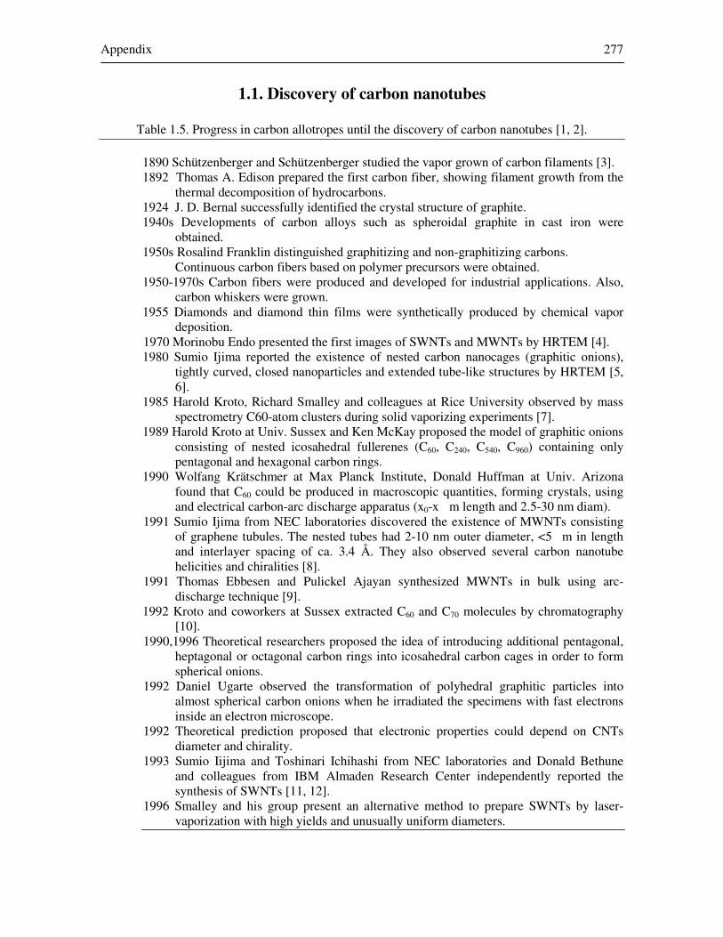
1.1. Discovery of carbon nanotubes
Table 1.5. Progress in carbon allotropes until the discovery of carbon nanotubes [1, 2]. 1890 Schützenberger and Schützenberger studied the vapor grown of carbon filaments [3]. 1892 Thomas A. Edison prepared the first carbon fiber, showing filament growth from the
thermal decomposition of hydrocarbons. 1924 J. D. Bernal successfully identified the crystal structure of graphite. 1940s Developments of carbon alloys such as spheroidal graphite in cast iron were
obtained. 1950s Rosalind Franklin distinguished graphitizing and non-graphitizing carbons. Continuous carbon fibers based on polymer precursors were obtained. 1950-1970s Carbon fibers were produced and developed for industrial applications. Also,
carbon whiskers were grown. 1955 Diamonds and diamond thin films were synthetically produced by chemical vapor
deposition. 1970 Morinobu Endo presented the first images of SWNTs and MWNTs by HRTEM [4]. 1980 Sumio Ijima reported the existence of nested carbon nanocages (graphitic onions),
tightly curved, closed nanoparticles and extended tube-like structures by HRTEM [5, 6].
1985 Harold Kroto, Richard Smalley and colleagues at Rice University observed by mass spectrometry C60-atom clusters during solid vaporizing experiments [7].
1989 Harold Kroto at Univ. Sussex and Ken McKay proposed the model of graphitic onions consisting of nested icosahedral fullerenes (C60, C240, C540, C960) containing only pentagonal and hexagonal carbon rings.
1990 Wolfang Krätschmer at Max Planck Institute, Donald Huffman at Univ. Arizona found that C60 could be produced in macroscopic quantities, forming crystals, using and electrical carbon-arc discharge apparatus (x0-x�m length and 2.5-30 nm diam).
1991 Sumio Ijima from NEC laboratories discovered the existence of MWNTs consisting of graphene tubules. The nested tubes had 2-10 nm outer diameter, <5�m in length and interlayer spacing of ca. 3.4 Å. They also observed several carbon nanotube helicities and chiralities [8].
1991 Thomas Ebbesen and Pulickel Ajayan synthesized MWNTs in bulk using arc-discharge technique [9].
1992 Kroto and coworkers at Sussex extracted C60 and C70 molecules by chromatography [10].
1990,1996 Theoretical researchers proposed the idea of introducing additional pentagonal, heptagonal or octagonal carbon rings into icosahedral carbon cages in order to form spherical onions.
1992 Daniel Ugarte observed the transformation of polyhedral graphitic particles into almost spherical carbon onions when he irradiated the specimens with fast electrons inside an electron microscope.
1992 Theoretical prediction proposed that electronic properties could depend on CNTs diameter and chirality.
1993 Sumio Iijima and Toshinari Ichihashi from NEC laboratories and Donald Bethune and colleagues from IBM Almaden Research Center independently reported the synthesis of SWNTs [11, 12].
1996 Smalley and his group present an alternative method to prepare SWNTs by laser-vaporization with high yields and unusually uniform diameters.
278
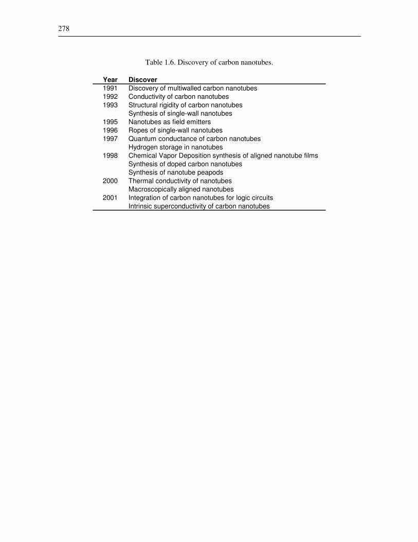
Table 1.6. Discovery of carbon nanotubes.
Year Discover
1991 Discovery of multiwalled carbon nanotubes
1992 Conductivity of carbon nanotubes
1993 Structural rigidity of carbon nanotubes
Synthesis of single-wall nanotubes
1995 Nanotubes as field emitters
1996 Ropes of single-wall nanotubes
1997 Quantum conductance of carbon nanotubes
Hydrogen storage in nanotubes
1998 Chemical Vapor Deposition synthesis of aligned nanotube films
Synthesis of doped carbon nanotubes
Synthesis of nanotube peapods
2000 Thermal conductivity of nanotubes
Macroscopically aligned nanotubes
2001 Integration of carbon nanotubes for logic circuits
Intrinsic superconductivity of carbon nanotubes
Appendix 279
1.2. Growth mechanisms of carbon nanotubes
The general mechanism of carbon nanotubes formation from chaotic carbon plasma, independently of the producing method, remains a great challenge. Nevertheless, many efforts have been devoted to model their growth behavior. In this section, some of the postulated theories will be presented in the case of the two main carbon nanotube production methods (i.e. arc discharge and pyrolysis). Growth mechanism of carbon nanotubes produced by electric-arc evaporation
method.
To explain the growth mechanism of carbon nanotubes produced by electric-arc evaporation, there are two main theories:
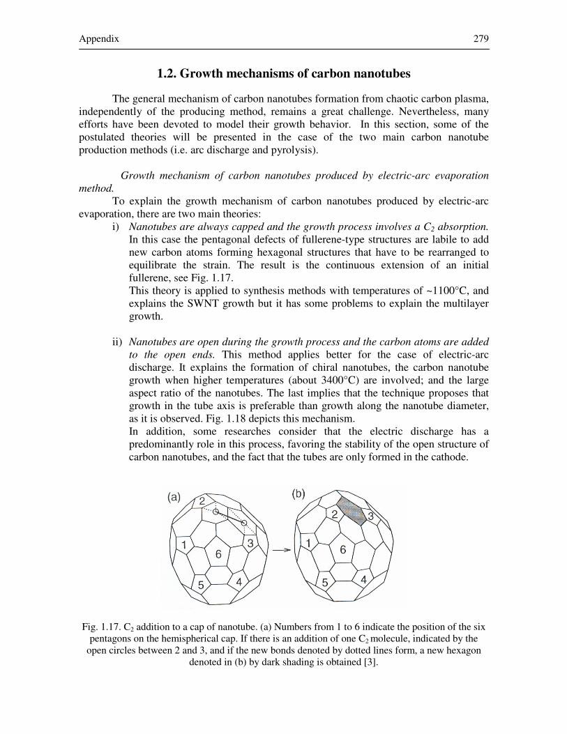
i) Nanotubes are always capped and the growth process involves a C2 absorption.
In this case the pentagonal defects of fullerene-type structures are labile to add new carbon atoms forming hexagonal structures that have to be rearranged to equilibrate the strain. The result is the continuous extension of an initial fullerene, see Fig. 1.17. This theory is applied to synthesis methods with temperatures of ~1100°C, and explains the SWNT growth but it has some problems to explain the multilayer growth.
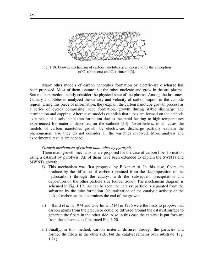
ii) Nanotubes are open during the growth process and the carbon atoms are added
to the open ends. This method applies better for the case of electric-arc discharge. It explains the formation of chiral nanotubes, the carbon nanotube growth when higher temperatures (about 3400°C) are involved; and the large aspect ratio of the nanotubes. The last implies that the technique proposes that growth in the tube axis is preferable than growth along the nanotube diameter, as it is observed. Fig. 1.18 depicts this mechanism. In addition, some researches consider that the electric discharge has a predominantly role in this process, favoring the stability of the open structure of carbon nanotubes, and the fact that the tubes are only formed in the cathode.
Fig. 1.17. C2 addition to a cap of nanotube. (a) Numbers from 1 to 6 indicate the position of the six pentagons on the hemispherical cap. If there is an addition of one C2 molecule, indicated by the
open circles between 2 and 3, and if the new bonds denoted by dotted lines form, a new hexagon denoted in (b) by dark shading is obtained [3].
280
Fig. 1.18. Growth mechanism of carbon nanotubes at an open end by the absorption of C2 (dimmers) and C3 (trimers) [3].
Many other models of carbon nanotubes formation by electric-arc discharge has
been proposed. Most of them assume that the tubes nucleate and grow in the arc plasma. Some others predominantly consider the physical state of the plasma. Among the last ones, Gamaly and Ebbesen analyzed the density and velocity of carbon vapors in the cathode region. Using this piece of information, they explain the carbon nanotube growth process as a series of cycles comprising: seed formation, growth during stable discharge and termination and capping. Alternative models establish that tubes are formed on the cathode as a result of a solid-state transformation due to the rapid heating to high temperatures experienced for material deposited on the cathode [13]. Nevertheless, in all cases the models of carbon nanotubes growth by electric-arc discharge partially explain the phenomenon; also they do not consider all the variables involved. More analysis and experimental results are needed.
Growth mechanism of carbon nanotubes by pyrolysis.
Three main growth mechanisms are proposed for the case of carbon fiber formation using a catalyst by pyrolysis. All of them have been extended to explain the SWNTs and MWNTs growth:
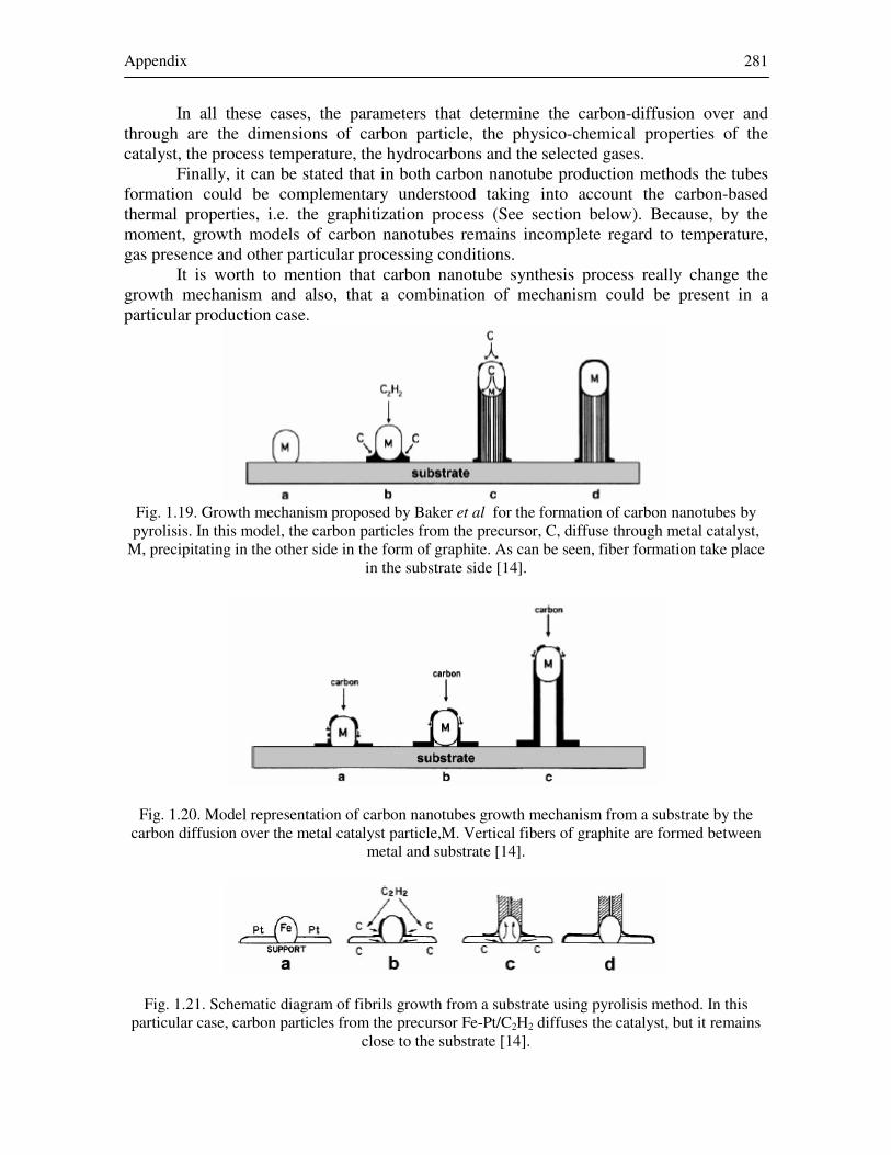
i) This mechanism was first proposed by Baker et al. In this case, fibers are produce by the diffusion of carbon (obtained from the decomposition of the hydrocarbon) through the catalyst with the subsequent precipitation and deposition on the other particle side (colder zone). The mechanism diagram is schemed in Fig. 1.19. As can be seen, the catalyst particle is separated from the substrate by the tube formation. Neutralization of the catalytic activity or the lack of carbon atoms determines the end of the growth.
ii) Baird et al in 1974 and Oberlin et al [4] in 1976 were the firsts to propose that
carbon atoms from the precursor could be diffused around the catalyst surface to generate the fibers in the other side. Also in this case the catalyst is put forward from the substrate, as illustrated Fig. 1.20.
iii) Finally, in this method, carbon material diffuses through the particles and
formed the fibers in the other side, but the catalyst remains over substrate (Fig. 1.21).
Appendix 281
In all these cases, the parameters that determine the carbon-diffusion over and through are the dimensions of carbon particle, the physico-chemical properties of the catalyst, the process temperature, the hydrocarbons and the selected gases.
Finally, it can be stated that in both carbon nanotube production methods the tubes formation could be complementary understood taking into account the carbon-based thermal properties, i.e. the graphitization process (See section below). Because, by the moment, growth models of carbon nanotubes remains incomplete regard to temperature, gas presence and other particular processing conditions.
It is worth to mention that carbon nanotube synthesis process really change the growth mechanism and also, that a combination of mechanism could be present in a particular production case.
Fig. 1.19. Growth mechanism proposed by Baker et al for the formation of carbon nanotubes by pyrolisis. In this model, the carbon particles from the precursor, C, diffuse through metal catalyst,
M, precipitating in the other side in the form of graphite. As can be seen, fiber formation take place in the substrate side [14].
Fig. 1.20. Model representation of carbon nanotubes growth mechanism from a substrate by the carbon diffusion over the metal catalyst particle,M. Vertical fibers of graphite are formed between
metal and substrate [14].
Fig. 1.21. Schematic diagram of fibrils growth from a substrate using pyrolisis method. In this particular case, carbon particles from the precursor Fe-Pt/C2H2 diffuses the catalyst, but it remains
close to the substrate [14].
282
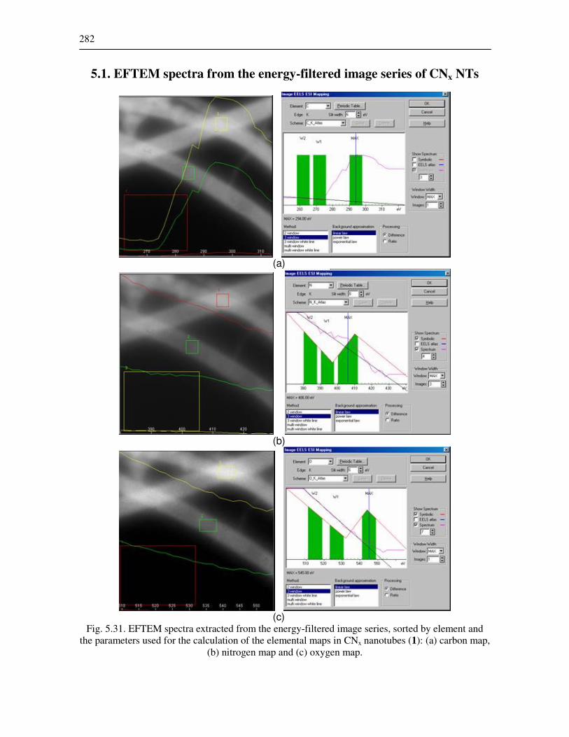
5.1. EFTEM spectra from the energy-filtered image series of CNx NTs
(a)
(b)
(c)
Fig. 5.31. EFTEM spectra extracted from the energy-filtered image series, sorted by element and the parameters used for the calculation of the elemental maps in CNx nanotubes (1): (a) carbon map,
(b) nitrogen map and (c) oxygen map.
Appendix 283
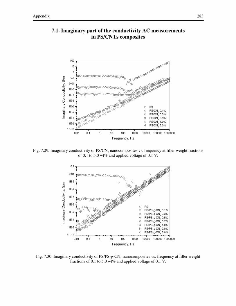
7.1. Imaginary part of the conductivity AC measurements
in PS/CNTs composites
0.01 0.1 1 10 100 1000 10000 100000 1000000
1E-10
1E-9
1E-8
1E-7
1E-6
1E-5
1E-4
1E-3
0.01
0.1
1
10
100
PS
PS/CNX 0.1%
PS/CNX 0.3%
PS/CNX 0.5%
PS/CNX 1.0%
PS/CNX 5.0%
Ima
gin
ary
Co
nd
uctivity,
S/m
Frequency, Hz
Fig. 7.29. Imaginary conductivity of PS/CNx nanocomposites vs. frequency at filler weight fractions
of 0.1 to 5.0 wt% and applied voltage of 0.1 V.
0.01 0.1 1 10 100 1000 10000 100000 1000000
1E-10
1E-9
1E-8
1E-7
1E-6
1E-5
1E-4
1E-3
0.01
0.1
PS
PS/PS-g-CNX 0.1%
PS/PS-g-CNX 0.3%
PS/PS-g-CNX 0.5%
PS/PS-g-CNX 0.7%
PS/PS-g-CNX 1.0%
PS/PS-g-CNX 2.0%
PS/PS-g-CNX 5.0%
Ima
gin
ary
Co
nd
uctivity,
S/m
Frequency, Hz
Fig. 7.30. Imaginary conductivity of PS/PS-g-CNx nanocomposites vs. frequency at filler weight
fractions of 0.1 to 5.0 wt% and applied voltage of 0.1 V.
284
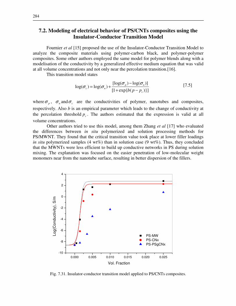
7.2. Modeling of electrical behavior of PS/CNTs composites using the
Insulator-Conductor Transition Model
Fournier et al [15] proposed the use of the Insulator-Conductor Transition Model to analyze the composite materials using polymer-carbon black, and polymer-polymer composites. Some other authors employed the same model for polymer blends along with a modelisation of the conductivity by a generalized effective medium equation that was valid at all volume concentrations and not only near the percolation transition.[16].
This transition model states
[7.5]
where pσ , nσ and cσ are the conductivities of polymer, nanotubes and composites,
respectively. Also b is an empirical parameter which leads to the change of conductivity at the percolation threshold cp . The authors estimated that the expression is valid at all volume concentrations. Other authors tried to use this model, among them Zhang et al [17] who evaluated the differences between in situ polymerized and solution processing methods for PS/MWNT. They found that the critical transition value took place at lower filler loadings in situ polymerized samples (4 wt%) than in solution case (9 wt%). Thus, they concluded that the MWNTs were less efficient to build up conductive networks in PS during solution mixing. The explanation was focused on the easier penetration of low-molecular weight monomers near from the nanotube surface, resulting in better dispersion of the fillers.
Fig. 7.31. Insulator-conductor transition model applied to PS/CNTs composites.
)}](exp{1[
)]log()[log()log()log(
c
np
ncppb −+
−
+=
σσ
σσ
0.000 0.005 0.010 0.015 0.020 0.025
-10
-8
-6
-4
-2
0
2
4
Lo
g(C
on
du
ctivity),
S/m
Vol. Fraction
PS-MW
PS-CNx
PS-PSgCNx
Appendix 285
Fig. 7.31 presents the experimental results for the conductivity vs. volume fraction of nanofillers of PS/MWNT, PS/CNx and PS/PS-g-CNx, and the fits obtained with the insulator-conductor transition model. The parameters pσ , nσ , cσ and pc were set and the
obtained parameter was b. It seemed that the Insulator-Conductor Transition Model describes approximately the conductivity of PS/MWNT, nevertheless as the carbon nanotube fillers were chemically modified by nitrogen doping and further by polymer-grafting, the experimental values were not correctly fitted. This result mainly means that as the nanotubes become more functionalized the influence of the contact becomes more important and deviates the result from that of the sum of their parts. Therefore, the insulator-conductor transition model is not appropriate to model all the PS/CNTs synthesized here.
286
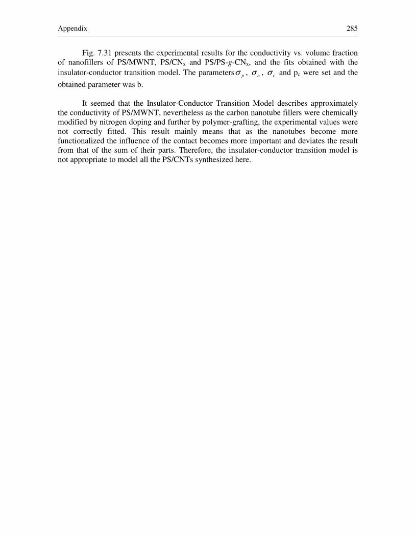
7.3. Conductivity exponent and the percolation threshold in PS/CNTs
composites calculated using the statistical percolation model
0.000 0.005 0.010 0.015 0.020 0.025
1E-9
1E-8
1E-7
1E-6
1E-5
1E-4
1E-3
0.01
0.1
1
10
100
1000
1.1
0015.01
0015.034538
−
−=
pe
σ
σe, S
/m
Vol. Fraction, p
-3.0 -2.5 -2.0 -1.5
1.2
1.4
1.6
1.8
2.0
2.2
2.4
2.6
2.8
3.0
σe,
S/m
Log(p-pc)
Fig. 7.32. Real part of the AC electrical conductivity at 1 Hz and applied voltage of 0.1 V for
PS/MWNT at several filler contents. Comparison with statistical percolation theory (solid lines).
0.000 0.005 0.010 0.015 0.020 0.025
1E-10
1E-9
1E-8
1E-7
1E-6
1E-5
1E-4
1E-3
0.01
0.1
1
10
100
1000
2.2
0015.01
0015.0741242
−
−=
peσ
σe,
S/m
Vol. Fraction, p
-4 -3 -2 -1
-2
-1
0
1
2
3
Lo
g(σ
e)
Log(p-pc)
Fig. 7.33. Real part of the AC electrical conductivity at 1 Hz and 0.1 V for PS/CNx at several filler
contents. Comparison with statistical percolation theory (solid lines).
Appendix 287
0.000 0.005 0.010 0.015 0.020 0.025 0.030
1E-11
1E-10
1E-9
1E-8
1E-7
1E-6
1E-5
1E-4
1E-3
0.01
0.1
1
10
σe, S
/m
Vol. Fraction, p
-3.0 -2.8 -2.6 -2.4 -2.2 -2.0 -1.8 -1.6-4
-2
0
2
6.3
0.0035-10.0035-p
2936973
=eσ
Log(σ
e)
Log(p-pc)
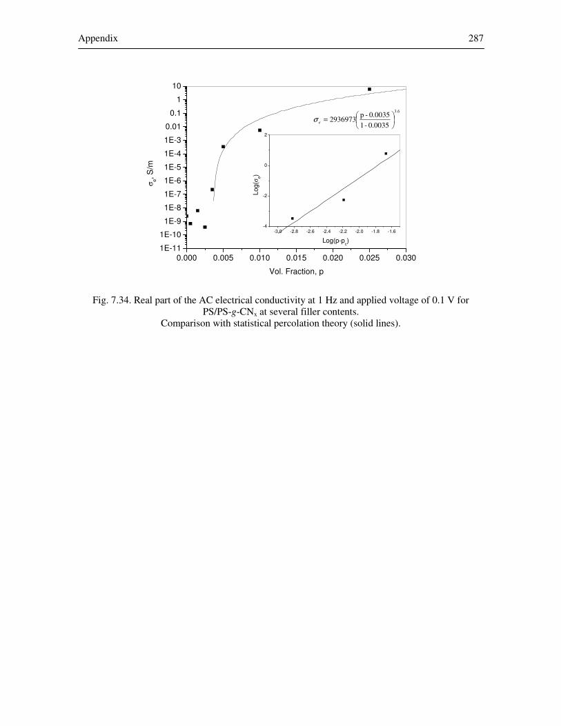
Fig. 7.34. Real part of the AC electrical conductivity at 1 Hz and applied voltage of 0.1 V for
PS/PS-g-CNx at several filler contents. Comparison with statistical percolation theory (solid lines).
288
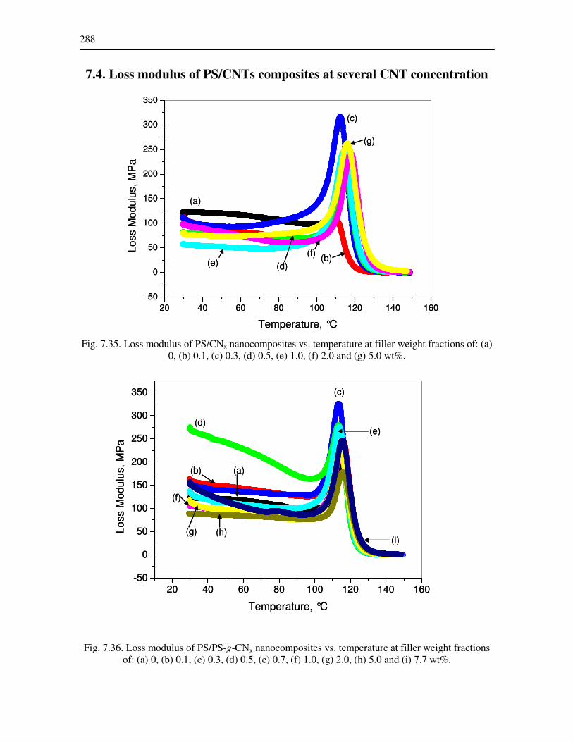
7.4. Loss modulus of PS/CNTs composites at several CNT concentration
Fig. 7.35. Loss modulus of PS/CNx nanocomposites vs. temperature at filler weight fractions of: (a)
0, (b) 0.1, (c) 0.3, (d) 0.5, (e) 1.0, (f) 2.0 and (g) 5.0 wt%.
Fig. 7.36. Loss modulus of PS/PS-g-CNx nanocomposites vs. temperature at filler weight fractions
of: (a) 0, (b) 0.1, (c) 0.3, (d) 0.5, (e) 0.7, (f) 1.0, (g) 2.0, (h) 5.0 and (i) 7.7 wt%.
20 40 60 80 100 120 140 160
-50
0
50
100
150
200
250
300
350
Loss M
od
ulu
s, M
Pa
Temperature, °C
(g)
(a)
(c)
(e)(b)
(d)
(f)
20 40 60 80 100 120 140 160
-50
0
50
100
150
200
250
300
350
Loss M
od
ulu
s, M
Pa
Temperature, °C
(g)
(a)
(c)
(e)(b)
(d)
(f)
20 40 60 80 100 120 140 160-50
0
50
100
150
200
250
300
350
Lo
ss M
od
ulu
s,
MP
a
Temperature, °C
(f)
(g) (h)
(d)
(i)
(b) (a)
(c)
(e)
20 40 60 80 100 120 140 160-50
0
50
100
150
200
250
300
350
Lo
ss M
od
ulu
s,
MP
a
Temperature, °C
(f)
(g) (h)
(d)
(i)
(b) (a)
(c)
(e)
Appendix 289
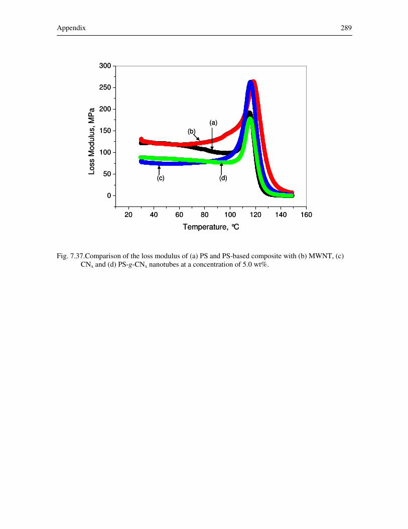
Fig. 7.37.Comparison of the loss modulus of (a) PS and PS-based composite with (b) MWNT, (c)
CNx and (d) PS-g-CNx nanotubes at a concentration of 5.0 wt%.
20 40 60 80 100 120 140 160
0
50
100
150
200
250
300
Loss M
od
ulu
s,
MP
a
Temperature, °C
(d)
(b)
(c)
(a)
20 40 60 80 100 120 140 160
0
50
100
150
200
250
300
Loss M
od
ulu
s,
MP
a
Temperature, °C
(d)
(b)
(c)
(a)
290
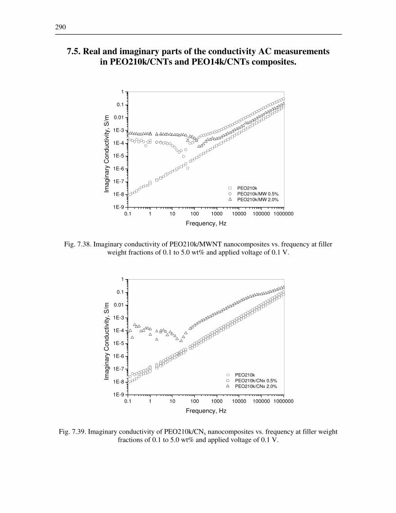
7.5. Real and imaginary parts of the conductivity AC measurements
in PEO210k/CNTs and PEO14k/CNTs composites.
0.1 1 10 100 1000 10000 100000 1000000
1E-9
1E-8
1E-7
1E-6
1E-5
1E-4
1E-3
0.01
0.1
1
Ima
gin
ary
Con
du
ctivity, S
/m
Frequency, Hz
PEO210k
PEO210k/MW 0.5%
PEO210k/MW 2.0%
Fig. 7.38. Imaginary conductivity of PEO210k/MWNT nanocomposites vs. frequency at filler
weight fractions of 0.1 to 5.0 wt% and applied voltage of 0.1 V.
0.1 1 10 100 1000 10000 100000 1000000
1E-9
1E-8
1E-7
1E-6
1E-5
1E-4
1E-3
0.01
0.1
1
Ima
gin
ary
Con
du
ctivity, S
/m
Frequency, Hz
PEO210k
PEO210k/CNx 0.5%
PEO210k/CNx 2.0%
Fig. 7.39. Imaginary conductivity of PEO210k/CNx nanocomposites vs. frequency at filler weight
fractions of 0.1 to 5.0 wt% and applied voltage of 0.1 V.
Appendix 291
0.1 1 10 100 1000 10000 100000 1000000
1E-9
1E-8
1E-7
1E-6
1E-5
1E-4
1E-3
0.01
0.1
Imagin
ary
Conductivity, S
/m
Frequency, Hz
PEO210k
PEO210k/PS-g-CNx 0.5%
PEO210k/PS-g-CNx 2.0%
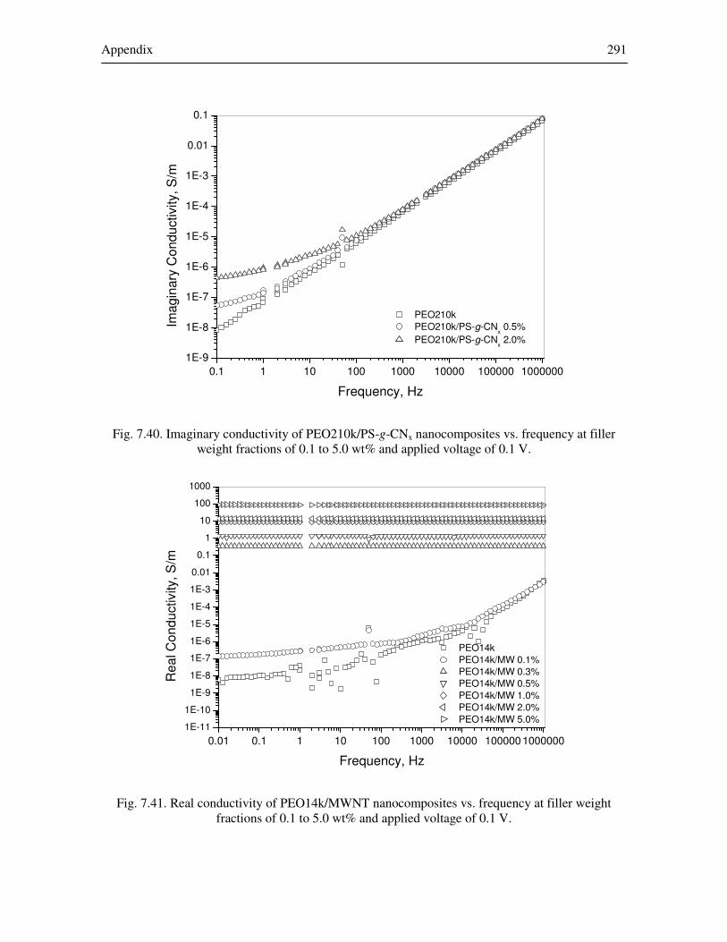
Fig. 7.40. Imaginary conductivity of PEO210k/PS-g-CNx nanocomposites vs. frequency at filler
weight fractions of 0.1 to 5.0 wt% and applied voltage of 0.1 V.
0.01 0.1 1 10 100 1000 10000 100000 1000000
1E-11
1E-10
1E-9
1E-8
1E-7
1E-6
1E-5
1E-4
1E-3
0.01
0.1
1
10
100
1000
PEO14k
PEO14k/MW 0.1%
PEO14k/MW 0.3%
PEO14k/MW 0.5%
PEO14k/MW 1.0%
PEO14k/MW 2.0%
PEO14k/MW 5.0%
Re
al C
on
du
ctivity, S
/m
Frequency, Hz
Fig. 7.41. Real conductivity of PEO14k/MWNT nanocomposites vs. frequency at filler weight
fractions of 0.1 to 5.0 wt% and applied voltage of 0.1 V.
292
0.01 0.1 1 10 100 1000 10000 100000 1000000
1E-9
1E-8
1E-7
1E-6
1E-5
1E-4
1E-3
0.01
0.1
1
10
Imagin
ary
Conductivity, S
/m
Frequency, Hz
PEO14k
PEO14k/MW 0.1%
PEO14k/MW 0.3%
PEO14k/MW 0.5%
PEO14k/MW 1.0%
PEO14k/MW 2.0%
PEO14k/MW 5.0%
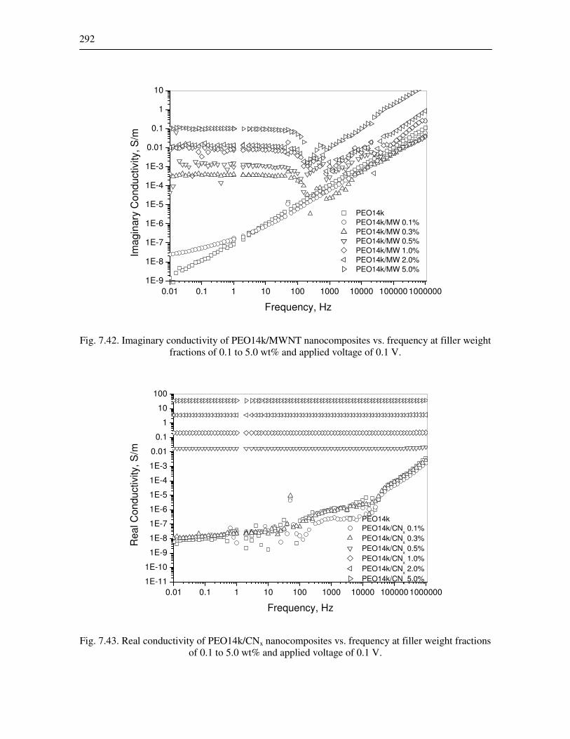
Fig. 7.42. Imaginary conductivity of PEO14k/MWNT nanocomposites vs. frequency at filler weight
fractions of 0.1 to 5.0 wt% and applied voltage of 0.1 V.
0.01 0.1 1 10 100 1000 10000 1000001000000
1E-11
1E-10
1E-9
1E-8
1E-7
1E-6
1E-5
1E-4
1E-3
0.01
0.1
1
10
100
Rea
l C
on
du
ctivity, S
/m
Frequency, Hz
PEO14k
PEO14k/CNx 0.1%
PEO14k/CNx 0.3%
PEO14k/CNx 0.5%
PEO14k/CNx 1.0%
PEO14k/CNx 2.0%
PEO14k/CNx 5.0%
Fig. 7.43. Real conductivity of PEO14k/CNx nanocomposites vs. frequency at filler weight fractions
of 0.1 to 5.0 wt% and applied voltage of 0.1 V.
Appendix 293
0.01 0.1 1 10 100 1000 10000 1000001000000
1E-10
1E-9
1E-8
1E-7
1E-6
1E-5
1E-4
1E-3
0.01
0.1
1
10
Ima
gin
ary
Con
du
ctivity, S
/m
Frequency, Hz
PEO14k
PEO14k/CNx 0.1%
PEO14k/CNx 0.3%
PEO14k/CNx 0.5%
PEO14k/CNx 1.0%
PEO14k/CNx 2.0%
PEO14k/CNx 5.0%
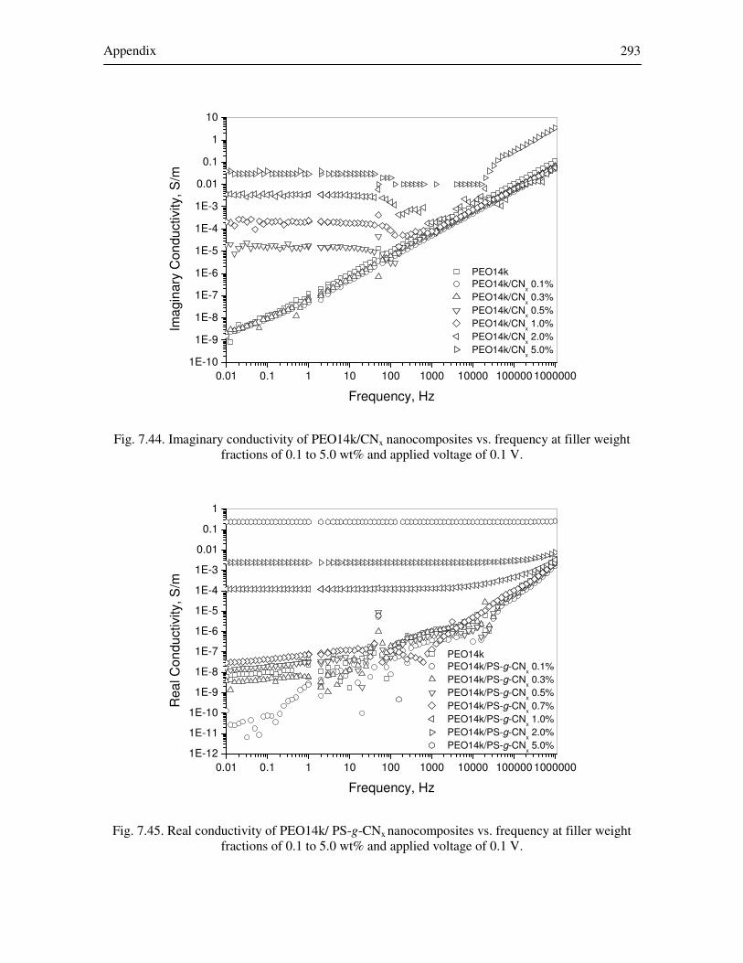
Fig. 7.44. Imaginary conductivity of PEO14k/CNx nanocomposites vs. frequency at filler weight
fractions of 0.1 to 5.0 wt% and applied voltage of 0.1 V.
0.01 0.1 1 10 100 1000 10000 1000001000000
1E-12
1E-11
1E-10
1E-9
1E-8
1E-7
1E-6
1E-5
1E-4
1E-3
0.01
0.1
1
Rea
l C
on
du
ctivity, S
/m
Frequency, Hz
PEO14k
PEO14k/PS-g-CNx 0.1%
PEO14k/PS-g-CNx 0.3%
PEO14k/PS-g-CNx 0.5%
PEO14k/PS-g-CNx 0.7%
PEO14k/PS-g-CNx 1.0%
PEO14k/PS-g-CNx 2.0%
PEO14k/PS-g-CNx 5.0%
Fig. 7.45. Real conductivity of PEO14k/ PS-g-CNx nanocomposites vs. frequency at filler weight
fractions of 0.1 to 5.0 wt% and applied voltage of 0.1 V.
294
0.01 0.1 1 10 100 1000 10000 1000001000000
1E-10
1E-9
1E-8
1E-7
1E-6
1E-5
1E-4
1E-3
0.01
0.1
Ima
gin
ary
Con
du
ctivity, S
/m
Frequency, Hz
PEO14k
PEO14k/PS-g-CNx 0.1%
PEO14k/PS-g-CNx 0.3%
PEO14k/PS-g-CNx 0.5%
PEO14k/PS-g-CNx 0.7%
PEO14k/PS-g-CNx 1.0%
PEO14k/PS-g-CNx 2.0%
PEO14k/PS-g-CNx 5.0%
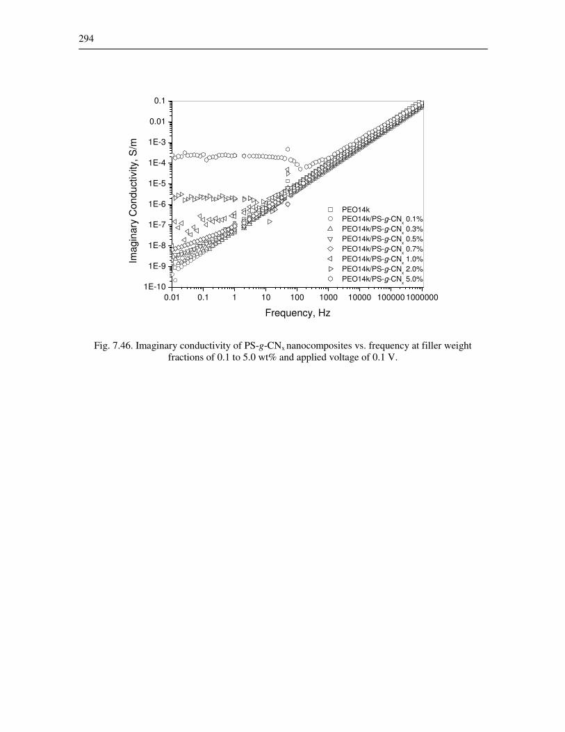
Fig. 7.46. Imaginary conductivity of PS-g-CNx nanocomposites vs. frequency at filler weight
fractions of 0.1 to 5.0 wt% and applied voltage of 0.1 V.
Appendix 295
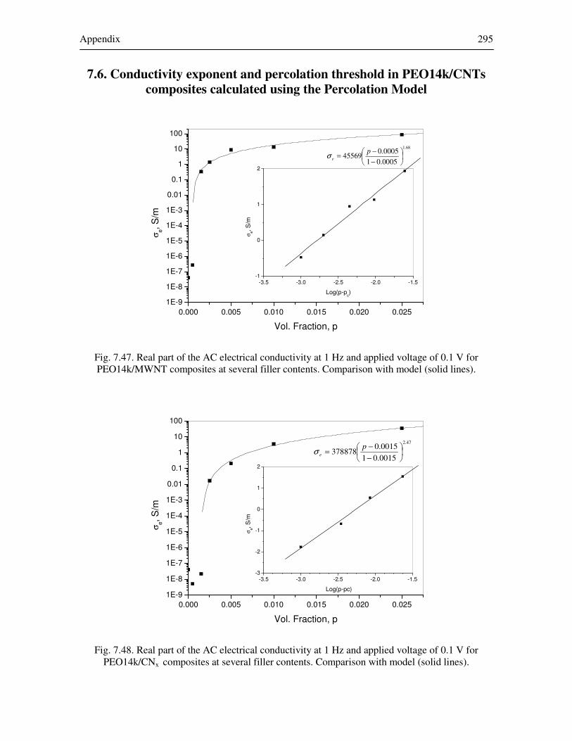
7.6. Conductivity exponent and percolation threshold in PEO14k/CNTs
composites calculated using the Percolation Model
0.000 0.005 0.010 0.015 0.020 0.025
1E-9
1E-8
1E-7
1E-6
1E-5
1E-4
1E-3
0.01
0.1
1
10
100
σe, S
/m
Vol. Fraction, p
-3.5 -3.0 -2.5 -2.0 -1.5-1
0
1
2
68.1
0005.010005.0
45569
−
−=
peσ
σe, S
/m
Log(p-pc)
Fig. 7.47. Real part of the AC electrical conductivity at 1 Hz and applied voltage of 0.1 V for PEO14k/MWNT composites at several filler contents. Comparison with model (solid lines).
0.000 0.005 0.010 0.015 0.020 0.025
1E-9
1E-8
1E-7
1E-6
1E-5
1E-4
1E-3
0.01
0.1
1
10
100
σe, S
/m
Vol. Fraction, p
-3.5 -3.0 -2.5 -2.0 -1.5-3
-2
-1
0
1
2
47.2
0015.010015.0
378878
−
−=
peσ
Log(p-pc)
σe, S
/m
Fig. 7.48. Real part of the AC electrical conductivity at 1 Hz and applied voltage of 0.1 V for
PEO14k/CNx composites at several filler contents. Comparison with model (solid lines).
296
0.000 0.005 0.010 0.015 0.020 0.025
1E-9
1E-8
1E-7
1E-6
1E-5
1E-4
1E-3
0.01
0.1
1
8.3
003.01
003.0609102
−
−=
peσ
σe,
S/m
Vol. Fraction, p
-3.5 -3.0 -2.5 -2.0 -1.5
-8
-6
-4
-2
0
σe, S
/m
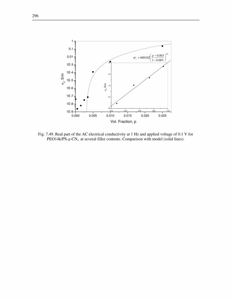
Fig. 7.49. Real part of the AC electrical conductivity at 1 Hz and applied voltage of 0.1 V for
PEO14k/PS-g-CNx at several filler contents. Comparison with model (solid lines).
Appendix 297
References
1. Terrones, M. and H. Terrones, The carbon nanocosmos: novel materials for the twenty-first
century. Philosophical Trans Royal Society of London A, 2003. 361: p. 2789-2806. 2. Subramoney, S., Novel nanocarbons-structure, properties and potential applications.
Advanced Materials, 1998. 10: p. 1157-1171. 3. Saito, R., G. Dresselhaus, and M.S. Dresselhaus, Physical properties of carbon nanotubes.
1998, London: Imperial College Press. 279. 4. Oberlin, A., M. Endo, and T. Koyama, Filamentous growth of carbon through benzene
decomposition. Journal of Crystal Growth, 1976. 32: p. 335-349. 5. Iijima, S., High resolution electron microscopy of some carbonaceous materials. Journal of
Microscopy, 1980. 119: p. 99. 6. Iijima, S., Direct observation of the tetrahedral bonding in graphitizing carbon black by
high-resolution electron microscopy. Journal of Crystal Growth, 1980. 50: p. 675. 7. Heath, H.W., J.R. Heath, S.C. O'Brien, S.C. Curl, and R.E. Smalley, C60 :
Buckminsterfullerene. Nature, 1985. 318(6042): p. 162-163. 8. Iijima, S., Helical microtubules of graphitic carbon. Nature, 1991. 354: p. 56. 9. Terrones, M., W.K. Hsu, H.W. Kroto, and D.R.M. Walton, Nanotubes: a revolution in
material science and electronics., in In Fullerenes and related structures: topics in
chemistry series, A. Hirsch, Editor. 1998, Springer: Berlin. p. 189. 10. Dresselhaus, M.S., G. Dresselhaus, and P.C. Eklund, Science of fullerenes and carbon
nanotubes, in Science of fullerenes and carbon nanotubes. 1996, San Diego: Academic. p. 1-505.
11. Iijima, S. and T. Ichihashi, Single-shell carbon nanotubes of 1 nm diameter. Nature, 1993. 363: p. 603.
12. Bethune, D.S., C.H. Kiang, M.S. de Vries, G. Gorman, R. Savoy, J. Vasquez, and R. Beyers, Cobalt-catalysed growth of carbon nanotubes with single-atomic-layers walls. Nature, 1993. 363: p. 605.
13. Harris, P.J.F., Carbon nanotubes and related structures New materials for the twenty-first
century. 2001, Cambridge: Cambridge University Press. 279. 14. Terrones, M., Science and Technology of the twenty-first century: synthesis, properties, and
applications of carbon nanotubes. Annual Reviews Materials Research, 2003. 33: p. 419-501.
15. Fournier, J., G. Boiteux, G. Seytre, and G. Marichy, Percolation network of polypyrrole in
conducting polymer-composites. Synthetic Metals, 1997. 84: p. 839-840. 16. Lafosse, X., Percolation and dielectric relaxation in polypyrrole-Teflon alloys. Synthetic
Metals, 1995. 68: p. 227-231. 17. Zhang, B., R.W. Fu, M.Q. Zhang, X.M. Dong, P.L. Lan, and J.S. Qiu, Preparation and
characterization of gas-sensitive composites from multi-walled carbon
nanotubes/polystyrene. Sensors and Actuators B, 2005. 109(2): p. 323-328.