Embed Size (px)
Citation preview
Poncet-Montanges, A., Cooper, J., Jones, D., Gaitonde, A., & Lemmens, Y.(2017). Frequency Domain Approach for Transonic Aerodynamic ModellingApplied to a Viscous Wing. In 58th AIAA/ASCE/AHS/ASC Structures,Structural Dynamics, and Materials Conference [AIAA 2017-0075]American Institute of Aeronautics and Astronautics Inc, AIAA. DOI:10.2514/6.2017-0075
Peer reviewed version
Link to published version (if available):10.2514/6.2017-0075
Link to publication record in Explore Bristol ResearchPDF-document
This is the author accepted manuscript (AAM). The final published version (version of record) is available onlinevia AIAA at http://arc.aiaa.org/doi/abs/10.2514/6.2017-0075. Please refer to any applicable terms of use of thepublisher.
University of Bristol - Explore Bristol ResearchGeneral rights
This document is made available in accordance with publisher policies. Please cite only the publishedversion using the reference above. Full terms of use are available:http://www.bristol.ac.uk/pure/about/ebr-terms
1
American Institute of Aeronautics and Astronautics
Frequency Domain Approach for Transonic Aerodynamic
Modelling applied to a Viscous Aircraft Model
Adrien Poncet-Montanges1, J.E. Cooper
2, D. Jones
3 and A.L. Gaitonde
4
University of Bristol, Queens Building, University Walk, Bristol, BS8 1TH, UK
Y. Lemmens5
Siemens Industry Software, Leuven, Belgium
This work introduces a method for the construction of a reduced order model in the
frequency domain. With input data obtained with the TAU linearized frequency domain
solver, the reduced order model shows a strong ability to reconstruct the full order
frequency response of a viscous aircraft configuration. Reduced order models have been
successfully created for different strips on the wing, the fuselage and the horizontal plane.
Nomenclature
α = angle of attack
α0 = amplitude of the pitching motion
αm = mean angle of the pitching motion
Cp = pressure coefficient
CL = lift coefficient
CD = Drag coefficient
CM = Pitching moment coefficient
Fz = Vertical force
MY = Pitching moment
k = Reduced frequency
U∞ = Freestream velocity
I. Introduction
omputational Fluid Dynamics (CFD) now has a wide range of validity where it gives highly accurate results
compared to wind tunnel experiments. It is extensively used in industry for steady analysis such as performance
studies. However, unsteady aerodynamics is also required for aircraft design and aeroelastic applications such as
flutter speed or limit cycle oscillation prediction. Whilst more powerful computers have enabled the application of
CFD for unsteady loads calculations, in practice the computational cost remains too high for routine use, especially
when it comes to viscous flows.
Reduced order models (ROMs) can be constructed that aim to decrease the CPU time for unsteady loads calculations
by capturing the dominant behaviour of the numerical model with a small number of degrees of freedom, whilst
1 Marie Curie Early Stage Research Fellow in Aircraft Loads. Email : [email protected]
2 Royal Academy of Engineering Airbus Sir George White Professor of Aerospace Engineering. AFAIAA.
3 Senior Lecturer, Department of Aerospace Engineering, University of Bristol, AIAA member.
4 Senior Lecturer, Department of Aerospace Engineering, University of Bristol, AIAA member
5 Sr Project Leader RTD, Digital Factory Division, Simulation & Test solutions. Siemens Industry Software.
C
2
American Institute of Aeronautics and Astronautics
retaining good accuracy and stability. These ROMs enable [1] the study of the system, and establishing control laws
to be simplified. Model order reduction can be achieved using different methods; these depend on the physics of the
system, the accuracy wanted and the information availability. The latest can be based on physical equations,
engineering problems, datasets and so on. For systems whose model is strongly linked to the physics, order
reduction can even be performed by hand, thinking about the independencies between the parameters; interpolation
can also be used.
While building a ROM, one technique is to define projection bases and spaces. The idea is to use linear algebra and
to construct a subspace orthogonal to the Krylov subspace; this can be performed thanks to the Gram-Schmidt
orthonormalization method. Since it can be unstable [2] a modified Gram-Schmidt can be used. In order to achieve
this, Arnoldi developed an iterative algorithm [3]. If the system matrix is Hermitian, the Lanczos method [4] is much
faster. It is based on the Arnoldi method, but as the system matrix is symmetric, the algorithm is much simpler and
the recurrence is shorter: each vector 𝑈𝑗+1 is directly calculated from the two previous ones 𝑈𝑗 and 𝑈𝑗−1. The
Lanczos algorithm can also be combined with a Padé approximation, for a method called Padé via Lanczos (PVL).
This method aims to preserve of the stability of the system. In fact, the reduced order modeling techniques using the
Padé approximation do not ensure this stability [5]. Other methods such as partial PVL [6] enable the poles and the
zeros of the reduced transfer function to be corrected; it leads to an enhanced stability. Antoulas [7] uses the
advantages of both Krylov subspaces and balanced truncation approaches. Finally, the Passive Reduced-order
Interconnect Macromodelling Algorithm, while using the Arnoldi method guarantees the preservation of passivity
and enables an enhanced accuracy [8].
An alternative analysis approach uses the system response due to different excitations to identify reduced matrices.
Several algorithms have been developed for model reduction using singular value decomposition (SVD) of a Hankel
matrix. The idea is to eliminate the states requiring a large amount of energy to be reached, or a large amount of
energy to be observed, as both correspond to small eigenvalues [9]. Grammians are introduced since they can be
used to quantify these amounts of energy. The reachability grammian quantifies the energy needed to bring a state to
a chosen value, whereas the observability grammian quantifies the energy provided by an observed state [10]. The
value of these grammians obviously depends on the basis on which they are calculated. In the case of a stable
system, a basis in the state space exists in which states that are difficult to reach are also difficult to observe.
Normally, the Hankel singular values decrease rapidly. The balanced truncation aims at truncating the modes that
are not reachable and observable. They correspond to the smallest Hankel singular values. The singular value
decomposition is well-conditioned, stable and can always work, but can be expensive to compute. It solves high-
dimensional Lyapunov equations [11] ; the storage required is of the order O(n²), while the number of operations is
of the order O(n3). Many balancing methods exist, such as stochastic balancing, bounded real balancing, positive
real balancing [12]. The frequency weighted balancing [13], can be useful if a good approximation is needed only in
a specific frequency range. However, the reduced model is not necessarily stable if both input and output are
weighted. These frequency weighted balancing methods have undertaken many improvements: the most recent one
guarantees stability and yields to a simple error bound [14]. Based on Markov parameters, the Padé approximation
(moment matching method) [15] has then been improved by Arnoldi and Lanczos [4] and is particularly
recommended in the case of high dimension systems.
The reduced order model developed in this paper falls into the second category of approach and is described in the
following section.
3
American Institute of Aeronautics and Astronautics
II. Reduced order model
For given flow conditions, the frequency response of the integrated aerodynamic coefficients obtained with a CFD
code is directly related to the frequency of the pitching motion. It is therefore appropriate to build a reduced order
model of the frequency response in the frequency domain instead of performing a classical reduction in the time
domain. After solving the system and transforming back into the continuous time space, it is possible to reconstruct
any motion in the time domain. The conversion between continuous and discrete time or frequency spaces is
achieved using a bilinear transform, as it is a bijective function from [0, π] to [0,∞].
The developed method gives accurate results when applied to a pitching airfoil in the transonic range, with no
shock-induced separation. It uses the Eigensystem Realization Algorithm [16], based on the singular value
decomposition to keep the dominant modes of the frequency response. The method proposed enables a model based
on experimental data to be built without knowing the system matrices.
As it needs equispaced input data in the discrete frequency domain, the choice of the sampling spacing is a key
element.
The equispaced discrete frequencies are defined by
ω̂𝑑(𝑘) = 𝑗 𝜋
𝑁, j ∈ [0 , N] (1)
where j is an integer between 0 and 𝜋, and ω̂𝑑(𝑘) is the corresponding discrete frequency.
The relationship to continuous frequencies as a result of the linking bilinear transformation is controlled by the
sampling time parameter T via
ω(k) = 2
𝑇 tan
ω̂𝑑(𝑘)
2 (2)
T has to be chosen such that the continuous reduced frequencies are in the range of interest for the model input. In
aerodynamics it corresponds to continuous reduced frequencies mostly in the interval [0.01,10]. As the discrete
frequency response is real, the discrete frequency domain between [0,π] can be extended to [π,2π] using the
conjugate of the impulse response coefficients Gd :
G𝑑(𝑘 + 𝑁) = G𝑑∗ (𝑁 − 𝑘) (3)
A singular value decomposition [17] of the Hankel matrix defined using the 2N-points inverse discrete Fourier
transform (IDFT) is performed. The model reduction is performed by keeping the largest singular values.
A discrete-time linear and stable MIMO model of n-th order, with r-input and m-output channels can be described
using the following state space representation
𝒙(𝑘 + 1) = 𝐴𝑑𝒙(𝑘) + 𝐵𝑑𝒖(𝑘)
𝒚(𝑘) = 𝐶𝑑𝒚(𝑘) + 𝐷𝑑𝒖(𝑘) (4)
𝒙(𝑡) ∈ ℝn represents the vector of different degrees of freedom (called state vector in control theory). It contains for
example the unknown physical variables, such as velocity, pressure, density. 𝒚(𝑡) ∈ ℝp and 𝒖(𝑡) ∈ ℝm respectively
represent the vector of the outputs of interest of the system, and the vector of inputs.
Another convenient notation is also used for a discrete-time model:
𝐺𝑑 ∶ (𝐴𝑑 𝐵𝑑
𝐶𝑑 𝐷𝑑) (5)
4
American Institute of Aeronautics and Astronautics
As far as a continuous-time is concerned, the matrices are written in this paper under the form
𝐺 ∶ (𝐴 𝐵𝐶 𝐷
) (6)
The reduced matrices �̂�𝑟 and �̂�𝑟 are calculated [18]. G can be written as
𝐺�̂� = �̂�𝑑(𝑧𝐼 − �̂�𝑑)−1�̂�𝑑 + �̂�𝑑 , 𝑧 ∈ ℂ (7)
The calculation of �̂�𝑟 and �̂�𝑟 is achieved by decomposing G in its real and imaginary parts.
Importantly the method provides a model reduction which is approximately balanced in the discrete space.
Furthermore as the bilinear transform below is used to map to the continuous domain, the final continuous time
model is also approximately balanced.
G can be transformed in a discrete-time system
�̂�𝑑(𝑧) = �̂�𝑑 + �̂�𝑑(𝑧𝐼 − �̂�𝑑)−1�̂�𝑑 (8)
using the bilinear transformation [19]:
�̂� = 2
𝑇 (𝐼 + �̂�𝑑)−1 (�̂�𝑑 − 𝐼) (9)
�̂� = 2
√𝑇(𝐼 + �̂�𝑑) �̂�𝑑 (10)
�̂� = 2
√𝑇 �̂�𝑑 (𝐼 + �̂�𝑑)−1 (11)
�̂� = �̂�𝑑 − �̂�𝑑 (𝐼 + �̂�𝑑)−1 �̂�𝑑 (12)
5
American Institute of Aeronautics and Astronautics
III. Viscous aircraft, numerical model and solver
A. Case of interest
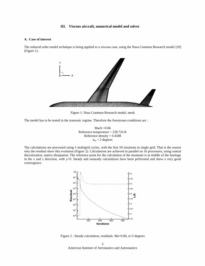
The reduced order model technique is being applied to a viscous case, using the Nasa Common Research model [20]
(Figure 1) .
Figure 1: Nasa Common Research model, mesh
The model has to be tested in the transonic regime. Therefore the freestream conditions are :
Mach =0.86
Reference temperature = 228.724 K
Reference density = 0.4588
αm = 2 degrees
The calculations are processed using 5 multigrid cycles, with the first 50 iterations in single grid. That is the reason
why the residual show this evolution (Figure 2). Calculations are achieved in parallel on 16 processors, using central
discretization, matrix dissipation. The reference point for the calculation of the moments is at middle of the fuselage
in the x and z direction, with y=0. Steady and unsteady calculations have been performed and show a very good
convergence.
Figure 2 : Steady calculation, residuals. Ma=0.86, α=2 degrees
6
American Institute of Aeronautics and Astronautics
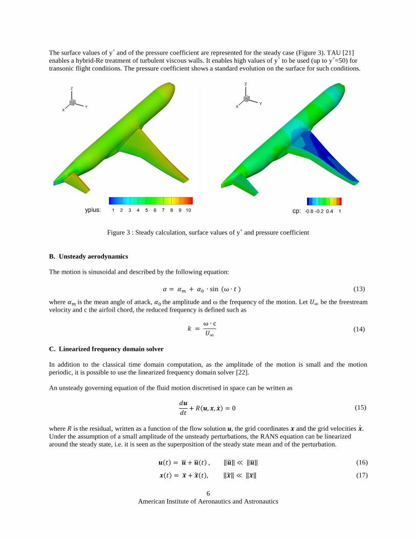
The surface values of y+ and of the pressure coefficient are represented for the steady case (Figure 3). TAU [21]
enables a hybrid-Re treatment of turbulent viscous walls. It enables high values of y+ to be used (up to y
+=50) for
transonic flight conditions. The pressure coefficient shows a standard evolution on the surface for such conditions.
Figure 3 : Steady calculation, surface values of y+ and pressure coefficient
B. Unsteady aerodynamics
The motion is sinusoidal and described by the following equation:
𝛼 = 𝛼𝑚 + 𝛼0 ∙ sin (ω ∙ 𝑡 ) (13)
where 𝛼𝑚 is the mean angle of attack, 𝛼0 the amplitude and ω the frequency of the motion. Let 𝑈∞ be the freestream
velocity and c the airfoil chord, the reduced frequency is defined such as
𝑘 = ω ∙ c
𝑈∞
(14)
C. Linearized frequency domain solver
In addition to the classical time domain computation, as the amplitude of the motion is small and the motion
periodic, it is possible to use the linearized frequency domain solver [22].
An unsteady governing equation of the fluid motion discretised in space can be written as
𝑑𝒖
𝑑𝑡+ 𝑅(𝒖, 𝒙, �̇�) = 0 (15)
where 𝑅 is the residual, written as a function of the flow solution u, the grid coordinates 𝒙 and the grid velocities �̇�.
Under the assumption of a small amplitude of the unsteady perturbations, the RANS equation can be linearized
around the steady state, i.e. it is seen as the superposition of the steady state mean and of the perturbation.
𝒖(𝑡) = �̅� + �̃�(𝑡) , ‖�̃�‖ ≪ ‖�̅�‖ (16)
𝒙(𝑡) = 𝒙 + 𝒙(𝑡), ‖𝒙‖ ≪ ‖𝒙‖ (17)
7
American Institute of Aeronautics and Astronautics
Since the perturbation is assumed to be periodic, it can be transformed in the frequency domain and expressed as
�̃�𝑘(𝑡) = ∑ 𝑅𝑒(�̂�𝑘
𝑘
𝑒𝑗𝑘𝜔𝑡) (18)
where �̂�𝑘 are the complex Fourier coefficients of the motion, 𝜔 the frequency, k the mode and j complex number
such as
𝑗 = √−1 (19)
After replacing the linearized values of u(t) and x(t) in (15), the following system is obtained
𝐴𝒙 = 𝑏 where 𝐴 = (
𝜕𝑅
𝜕𝑢−𝜔𝐼
𝜔𝐼𝜕𝑅
𝜕𝑢
) and 𝑏 = (
𝜕𝑅
𝜕𝑥−𝜔
𝜕𝑅
𝜕�̇�
𝜔𝜕𝑅
𝜕�̇�
𝜕𝑅
𝜕𝑥
) (�̃�𝑅𝑒
�̃�𝐼𝑚) (20)
The Jacobian 𝜕𝑅/𝜕𝑢 is calculated analytically in TAU, but the right hand term is evaluated by using central finite
differences.
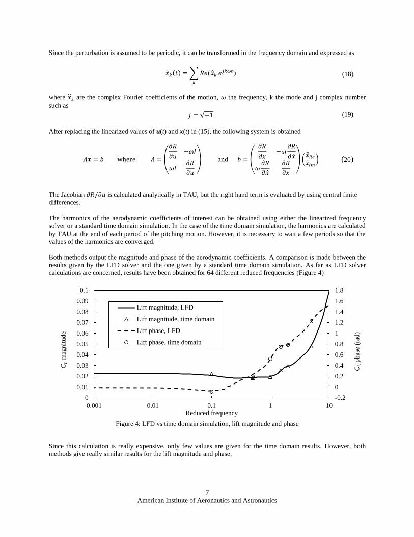
The harmonics of the aerodynamic coefficients of interest can be obtained using either the linearized frequency
solver or a standard time domain simulation. In the case of the time domain simulation, the harmonics are calculated
by TAU at the end of each period of the pitching motion. However, it is necessary to wait a few periods so that the
values of the harmonics are converged.
Both methods output the magnitude and phase of the aerodynamic coefficients. A comparison is made between the
results given by the LFD solver and the one given by a standard time domain simulation. As far as LFD solver
calculations are concerned, results have been obtained for 64 different reduced frequencies (Figure 4)
Figure 4: LFD vs time domain simulation, lift magnitude and phase
Since this calculation is really expensive, only few values are given for the time domain results. However, both
methods give really similar results for the lift magnitude and phase.
-0.2
0
0.2
0.4
0.6
0.8
1
1.2
1.4
1.6
1.8
0
0.01
0.02
0.03
0.04
0.05
0.06
0.07
0.08
0.09
0.1
0.001 0.01 0.1 1 10
CL p
has
e (r
ad)
CL m
agnit
ud
e
Reduced frequency
Lift magnitude, LFD
Lift magnitude, time domain
Lift phase, LFD
Lift phase, time domain
8
American Institute of Aeronautics and Astronautics
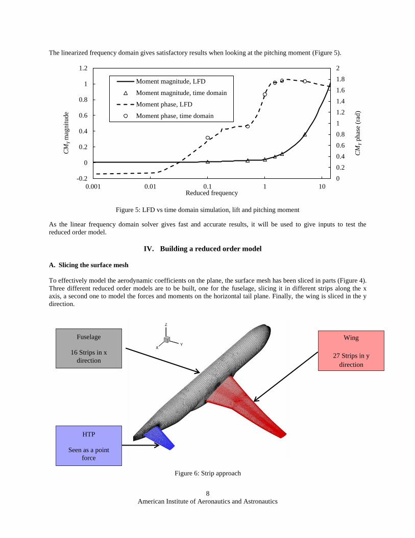
The linearized frequency domain gives satisfactory results when looking at the pitching moment (Figure 5).
Figure 5: LFD vs time domain simulation, lift and pitching moment
As the linear frequency domain solver gives fast and accurate results, it will be used to give inputs to test the
reduced order model.
IV. Building a reduced order model
A. Slicing the surface mesh
To effectively model the aerodynamic coefficients on the plane, the surface mesh has been sliced in parts (Figure 4).
Three different reduced order models are to be built, one for the fuselage, slicing it in different strips along the x
axis, a second one to model the forces and moments on the horizontal tail plane. Finally, the wing is sliced in the y
direction.
Figure 6: Strip approach
0
0.2
0.4
0.6
0.8
1
1.2
1.4
1.6
1.8
2
-0.2
0
0.2
0.4
0.6
0.8
1
1.2
0.001 0.01 0.1 1 10
CM
Y p
has
e (r
ad)
CM
Y m
agnit
ud
e
Reduced frequency
Moment magnitude, LFD
Moment magnitude, time domain
Moment phase, LFD
Moment phase, time domain
HTP
Seen as a point
force
Wing
27 Strips in y
direction
Fuselage
16 Strips in x
direction
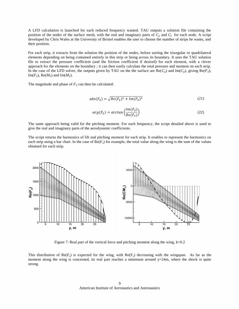
9
American Institute of Aeronautics and Astronautics
A LFD calculation is launched for each reduced frequency wanted. TAU outputs a solution file containing the
position of the nodes of the surface mesh, with the real and imaginary parts of Cp and Cf for each node. A script
developed by Chris Wales at the University of Bristol enables the user to choose the number of strips he wants, and
their position.
For each strip, it extracts from the solution the position of the nodes, before sorting the triangular or quadrilateral
elements depending on being contained entirely in this strip or being across its boundary. It uses the TAU solution
file to extract the pressure coefficient (and the friction coefficient if desired) for each element, with a clever
approach for the elements on the boundary ; it can then easily calculate the total pressure and moment on each strip.
In the case of the LFD solver, the outputs given by TAU on the the surface are Re(Cp) and Im(Cp), giving Re(FZ),
Im(FZ), Re(MY) and Im(MY).
The magnitude and phase of FZ can then be calculated:
𝑎𝑏𝑠(𝐹𝑍) = √𝑅𝑒(𝐹𝑍)2 + 𝐼𝑚(𝐹𝑍)2 (21)
𝑎𝑟𝑔(𝐹𝑍) = 𝑎𝑟𝑐𝑡𝑎𝑛 (𝐼𝑚(𝐹𝑍)
𝑅𝑒(𝐹𝑍)) (22)
The same approach being valid for the pitching moment. For each frequency, the script detailed above is used to
give the real and imaginary parts of the aerodynamic coefficients.
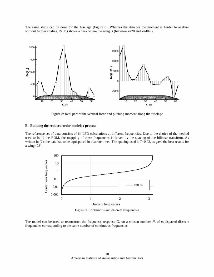
The script returns the harmonics of lift and pitching moment for each strip. It enables to represent the harmonics on
each strip using a bar chart. In the case of Re(Fz) for example, the total value along the wing is the sum of the values
obtained for each strip.
Figure 7: Real part of the vertical force and pitching moment along the wing, k=0.2
This distribution of Re(Fz) is expected for the wing, with Re(Fz) decreasing with the wingspan. As far as the
moment along the wing is concerned, its real part reaches a minimum around y=24m, where the shock is quite
strong.
10
American Institute of Aeronautics and Astronautics
The same study can be done for the fuselage (Figure 8). Whereas the data for the moment is harder to analyze
without further studies, Re(Fz) shows a peak where the wing is (between x=20 and x=40m).
Figure 8: Real part of the vertical force and pitching moment along the fuselage
B. Building the reduced order models : process
The reference set of data consists of 64 LFD calculations at different frequencies. Due to the choice of the method
used to build the ROM, the mapping of these frequencies is driven by the spacing of the bilinear transform. As
written in (2), the data has to be equispaced in discrete time. The spacing used is T=0.02, as gave the best results for
a wing [23].
Figure 9: Continuous and discrete frequencies
The model can be used to reconstruct the frequency response Gr on a chosen number Nr of equispaced discrete
frequencies corresponding to the same number of continuous frequencies.
0.001
0.01
0.1
1
10
100
0 1 2 3
Co
nti
nuo
us
freq
uen
cies
Discrete frequencies
T=0.02
11
American Institute of Aeronautics and Astronautics
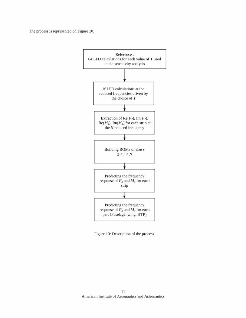
The process is represented on Figure 10.
Figure 10: Description of the process
N LFD calculations at the
reduced frequencies driven by
the choice of T
Extraction of Re(FZ), Im(FZ),
Re(MY), Im(MY) for each strip at
the N reduced frequency
Building ROMs of size r
2 < r < N
Predicting the frequency
response of FZ and MY for each
strip
Reference :
64 LFD calculations for each value of T used
in the sensitivity analysis
Predicting the frequency
response of FZ and MY for each
part (Fuselage, wing, HTP)
12
American Institute of Aeronautics and Astronautics
V. Results
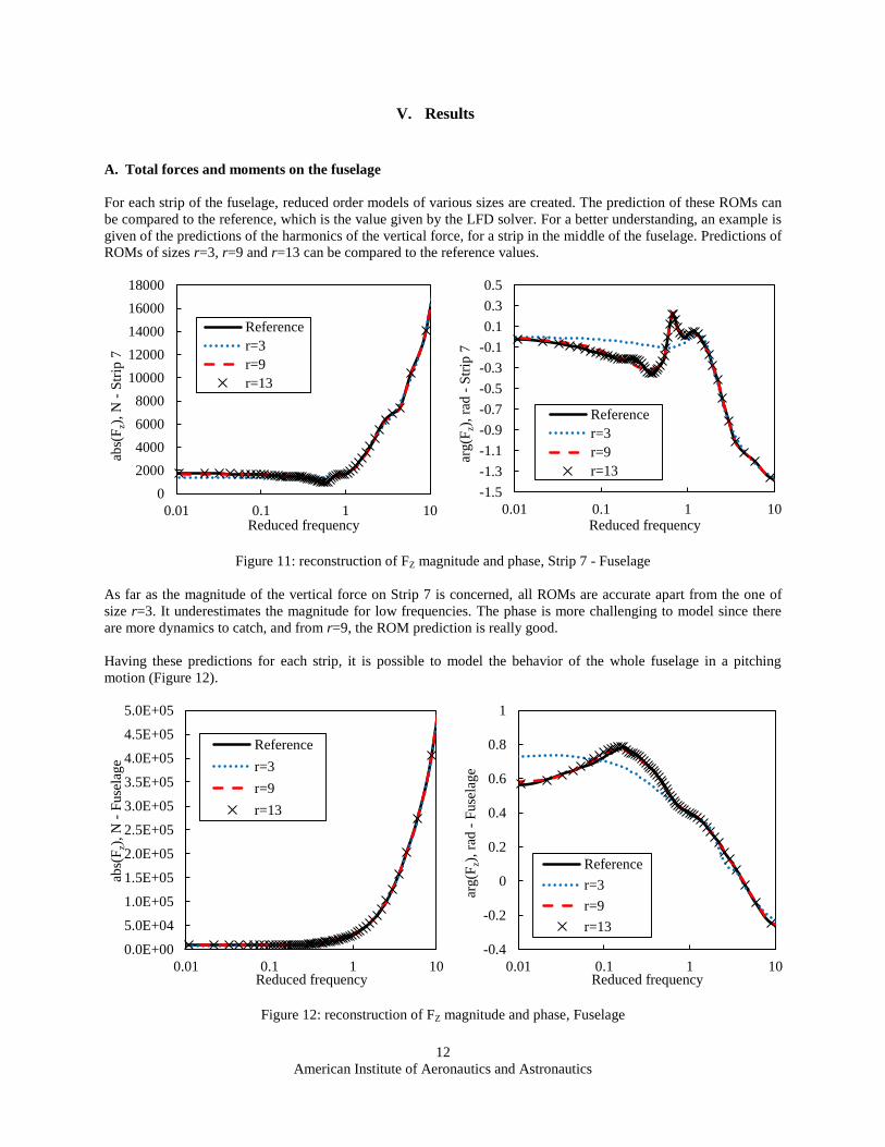
A. Total forces and moments on the fuselage
For each strip of the fuselage, reduced order models of various sizes are created. The prediction of these ROMs can
be compared to the reference, which is the value given by the LFD solver. For a better understanding, an example is
given of the predictions of the harmonics of the vertical force, for a strip in the middle of the fuselage. Predictions of
ROMs of sizes r=3, r=9 and r=13 can be compared to the reference values.
Figure 11: reconstruction of FZ magnitude and phase, Strip 7 - Fuselage
As far as the magnitude of the vertical force on Strip 7 is concerned, all ROMs are accurate apart from the one of
size r=3. It underestimates the magnitude for low frequencies. The phase is more challenging to model since there
are more dynamics to catch, and from r=9, the ROM prediction is really good.
Having these predictions for each strip, it is possible to model the behavior of the whole fuselage in a pitching
motion (Figure 12).
Figure 12: reconstruction of FZ magnitude and phase, Fuselage
0
2000
4000
6000
8000
10000
12000
14000
16000
18000
0.01 0.1 1 10
abs(
Fz)
, N
- S
trip
7
Reduced frequency
Reference
r=3
r=9
r=13
-1.5
-1.3
-1.1
-0.9
-0.7
-0.5
-0.3
-0.1
0.1
0.3
0.5
0.01 0.1 1 10
arg(F
z),
rad
- S
trip
7
Reduced frequency
Reference
r=3
r=9
r=13
0.0E+00
5.0E+04
1.0E+05
1.5E+05
2.0E+05
2.5E+05
3.0E+05
3.5E+05
4.0E+05
4.5E+05
5.0E+05
0.01 0.1 1 10
abs(
Fz)
, N
- F
use
lage
Reduced frequency
Reference
r=3
r=9
r=13
-0.4
-0.2
0
0.2
0.4
0.6
0.8
1
0.01 0.1 1 10
arg(F
z),
rad
- F
use
lage
Reduced frequency
Reference
r=3
r=9
r=13
13
American Institute of Aeronautics and Astronautics
The fuselage is a complex part since the variations in pressure coefficient between the different strips can be really
high. However, for both magnitude and phase, small ROMs (r=9) give an accurate prediction of the aerodynamic
coefficient.
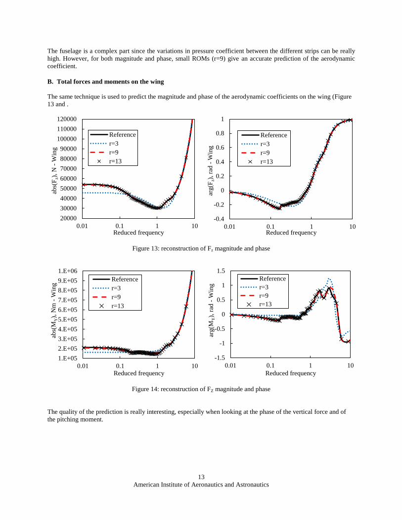
B. Total forces and moments on the wing
The same technique is used to predict the magnitude and phase of the aerodynamic coefficients on the wing (Figure
13 and .
Figure 13: reconstruction of Fz magnitude and phase
Figure 14: reconstruction of FZ magnitude and phase
The quality of the prediction is really interesting, especially when looking at the phase of the vertical force and of
the pitching moment.
20000
30000
40000
50000
60000
70000
80000
90000
100000
110000
120000
0.01 0.1 1 10
abs(
Fz)
, N
- W
ing
Reduced frequency
Reference
r=3
r=9
r=13
-0.4
-0.2
0
0.2
0.4
0.6
0.8
1
0.01 0.1 1 10
arg(F
z),
rad
- W
ing
Reduced frequency
Reference
r=3
r=9
r=13
1.E+05
2.E+05
3.E+05
4.E+05
5.E+05
6.E+05
7.E+05
8.E+05
9.E+05
1.E+06
0.01 0.1 1 10
abs(
MY),
Nm
- W
ing
Reduced frequency
Reference
r=3
r=9
r=13
-1.5
-1
-0.5
0
0.5
1
1.5
0.01 0.1 1 10
arg(M
Y),
rad
- W
ing
Reduced frequency
Reference
r=3
r=9
r=13
14
American Institute of Aeronautics and Astronautics
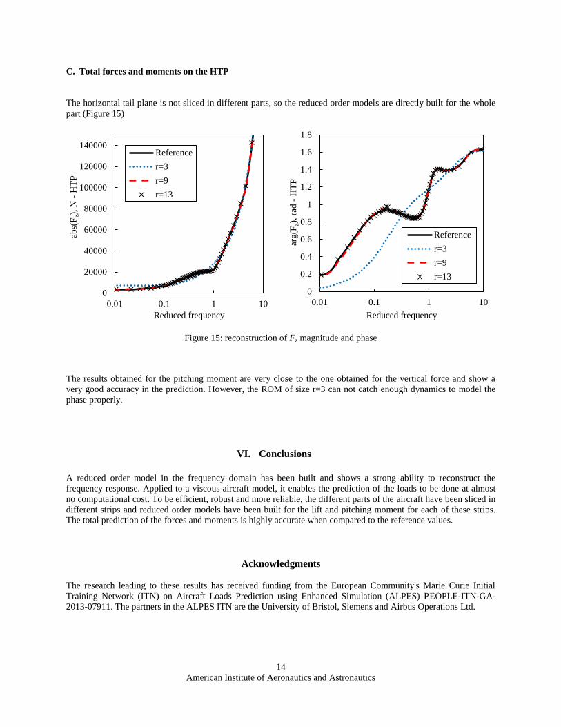
C. Total forces and moments on the HTP
The horizontal tail plane is not sliced in different parts, so the reduced order models are directly built for the whole
part (Figure 15)
Figure 15: reconstruction of Fz magnitude and phase
The results obtained for the pitching moment are very close to the one obtained for the vertical force and show a
very good accuracy in the prediction. However, the ROM of size r=3 can not catch enough dynamics to model the
phase properly.
VI. Conclusions
A reduced order model in the frequency domain has been built and shows a strong ability to reconstruct the
frequency response. Applied to a viscous aircraft model, it enables the prediction of the loads to be done at almost
no computational cost. To be efficient, robust and more reliable, the different parts of the aircraft have been sliced in
different strips and reduced order models have been built for the lift and pitching moment for each of these strips.
The total prediction of the forces and moments is highly accurate when compared to the reference values.
Acknowledgments
The research leading to these results has received funding from the European Community's Marie Curie Initial
Training Network (ITN) on Aircraft Loads Prediction using Enhanced Simulation (ALPES) PEOPLE-ITN-GA-
2013-07911. The partners in the ALPES ITN are the University of Bristol, Siemens and Airbus Operations Ltd.
0
20000
40000
60000
80000
100000
120000
140000
0.01 0.1 1 10
abs(
Fz)
, N
- H
TP
Reduced frequency
Reference
r=3
r=9
r=13
0
0.2
0.4
0.6
0.8
1
1.2
1.4
1.6
1.8
0.01 0.1 1 10ar
g(F
z),
rad
- H
TP
Reduced frequency
Reference
r=3
r=9
r=13
15
American Institute of Aeronautics and Astronautics
References
[1]
W. H. Schilders, H. A. Van der Vorst and J. Rommes, Model order reduction: theory, research aspects and
applications, vol. 13, Berlin: Springer, 2008.
[2] Å. Björck, "Solving linear least squares problems by Gram-Schmidt orthogonalization," BIT Numerical
Mathematics, vol. 7, no. 1, pp. 1-21, 1967.
[3] W. E. Arnoldi, "The principle of minimized iterations in the solution of the matrix eigenvalue problem,"
Quarterly of Applied Mathematics, vol. 9, no. 1, pp. 17-29, 1951.
[4] C. Lanczos, "An iteration method for the solution of the eigenvalue problem of linear differential and integral
operators," United States Governm. Press Office, 1950.
[5] Y. Shamash, "Stable reduced-order models using Padé-type approximation," Automatic Control, IEEE
Transactions on, vol. 19, no. 5, pp. 615-616, 1974.
[6] Z. Bai and R. W. Freund, "A partial Padé-via-Lanczos method for reduced-order modeling," Linear Algebra
and its Applications, vol. 332, pp. 139-164, 2001.
[7] A. C. Antoulas, "An overview of approximation methods for large-scale dynamical systems," Annual reviews
in Control, vol. 29, no. 2, pp. 181-190, 2005.
[8] A. Odabasioglu, M. Celik and L. T. Pileggi, "PRIMA : Passive reduced-order interconnect macromodeling
algorithm," in Proceedings of the 1997 IEEE/ACM international conference on Computer-aided design, IEEE
Computer Society, 1997, pp. 58-65.
[9] A. C. Antoulas, Approximation of large-scale dynamical systems, Siam, 2005.
[10] B. Moore, "Principal component analysis in linear systems: Controllability, observability, and model
reduction," Automatic control, vol. 26, no. 1, pp. 17-32, 1981.
[11] A. M. Lyapunov, "The general problem of the stability of motion," International Journal of Control, vol. 55,
no. 3, pp. 531-534, 1992.
[12] S. Gugercin and A. C. Antoulas, "A survey of model reduction by balanced truncation and some new results,"
International Journal of Control, vol. 77, no. 8, pp. 748-766, 2004.
[13] D. F. Enns, "Model reduction with balanced realizations: An error bound and a frequency weighted
generalization.," in Decision and Control, 1984. The 23rd IEEE Conference on, IEEE, 1984, pp. 127-132.
[14] G. Wang, V. Sreeram and W. Q. Liu, "A new frequency-weighted balanced truncation method and an error
bound," IEEE Transactions on Automatic Control, vol. 44, no. 9, pp. 1734-1737, 1999.
[15] P. Feldmann and R. W. Freund, "Efficient linear circuit analysis by Padé approximation via the Lanczos
process," Computer-Aided Design of Integrated Circuits and Systems, IEEE Transactions on, vol. 14, no. 5,
pp. 639-649, 1995.
[16] J.-N. Juang and R. S. Pappa, "An eigensystem realization algorithm for modal parameter identification and
model reduction," Journal of guidance, control, and dynamics, vol. 8, no. 5, pp. 620-627, 1985.
[17] G. H. Golub and C. Reinsch, "Singular value decomposition and least squares solutions," Numerische
Mathematik, vol. 14, no. 5, pp. 403-420, 1970.
[18] T. McKelvey, H. Akçay and L. Ljung, "Subspace-based multivariable system identification from frequency
response data," Automatic Control, IEEE Transactions on, vol. 41, no. 7, pp. 960-979, 1996.
[19] U. M. Al-Saggaf and G. F. Franklin, "Model reduction via balanced realizations: an extension and frequency
weighting techniques," Automatic Control, IEEE Transactions on, vol. 33, no. 7, pp. 687-692, 1988.

16
American Institute of Aeronautics and Astronautics
[20] J. C. VASSBERG, M. A. DEHAAN, S. M. RIVERS and e. al, " Development of a common research model
for applied CFD validation studies.," vol. 6919, p. 2008, 2008.
[21] D. Schwamborn, T. Gerhold and R. Heinrich, "The DLR TAU-code: Recent applications in research and
industry," in ECCOMAS CFD 2006: Proceedings of the European Conference on Computational Fluid
Dynamics, Egmond aan Zee, The Netherlands, September 5-8, 2006, Delft University of Technology,
European Community on Computational Methods in Applied Sciences (ECCOMAS), 2006.
[22] M. Widhalm, R. P. Dwight, R. Thormann and A. Hübner, "Efficient computation of dynamic stability data
with a linearized frequency domain solver," in European Conference on Computational Fluid Dynamics, 2010.
[23] A. Poncet-Montanges, J. Cooper, D. Jones and Y. Lemmens, "Frequency‐domain approach for transonic
unsteady aerodynamic modelling," in SciTech , San Diego, 2016.