Embed Size (px)
Citation preview
PONTIFÍCIA UNIVERSIDADE CATÓLICA DO RIO GRANDE DO S UL
FACULDADE DE BIOCIÊNCIAS
PROGRAMA DE PÓS-GRADUAÇÃO EM ZOOLOGIA
Modelagem da adequabilidade de hábitat de Corbicula fluminea
(Bivalvia, Corbiculidae), Pimelodus pintado e Parapimelodus nigribarbis
(Siluriformes, Pimelodidae) e Loricariichthys anus (Siluriformes,
Loricariidae) em relação a preditores ambientais no Lago Guaíba, RS,
Brasil
Me. Thiago Cesar Lima Silveira
Orientador: Dr. Nelson Ferreira Fontoura
TESE DE DOUTORADO
PORTO ALEGRE – RS – BRASIL
2015

II
SUMÁRIO
1 MODELOS ESTATÍSTICOS PARA A MODELAGEM DE DISTRIBUIÇÃO
ESPACIAL .................................................................................................................... 6
1.1 MODELOS SOMENTE COM DADOS DE PRESENÇA ........................................................... 8
1.1.1 ENFA (Ecological Niche Factor Analysis) ................................................................... 8
1.1.2 BIOCLIM .................................................................................................................... 8
1.1.3 DOMAIN .................................................................................................................... 9
1.1.4 GARP ......................................................................................................................... 9
1.1.5 MAXENT .................................................................................................................... 9
1.2 MODELOS COM DADOS DE PRESENÇA E AUSÊNCIA...................................................... 10
1.2.1 Árvores de classificação e regressão CART ............................................................. 10
1.2.2 Boosted regression Trees (BRT) .............................................................................. 10
1.2.3 Multivariate Adaptative Regression Splines (MARS) .............................................. 11
1.2.4 Modelos Lineares Generalizados (GLM) ................................................................. 11
1.2.5 Regressão logística .................................................................................................. 12
1.2.6 Modelos Aditivos Generalizados (GAM) ................................................................. 12
1.2.7 Redes Neurais Artificiais (RNA) ............................................................................... 13
1.3 CONSIDERAÇÕES SOBRE A ESCOLHA DA METODOLOGIA DE MODELAGEM ................. 14
2 O LAGO GUAÍBA .................................................................................................. 16
3 ORGANISMOS AQUÁTICOS ESTUDADOS ........................................................ 20
4 JUSTIFICATIVA .................................................................................................... 24
5 OBJETIVOS .......................................................................................................... 25
5.1 OBJETIVO GERAL ............................................................................................................ 25
5.2 OBJETIVOS ESPECÍFICOS ................................................................................................ 25

III
Aos que me apoiaram e incentivaram.

IV
“Prediction is very difficult, especially about the future.”
Niels Bohr

V
AGRADECIMENTOS
Após quatro anos de atividades na PUCRS, desempenhando minhas funções
como estudante de pós-graduação no Programa de Pós-graduação em Zoologia,
tenho que agradecer a inúmeras pessoas, que sem elas seria muito mais difícil
concluir esta etapa. Primeiramente agradeço ao meu orientador, Dr. Nelson Ferreira
Fontoura, por ter me aceitado como estudante de Doutorado em seu grupo de
pesquisa. Agradeço por todas as aulas, conselhos, incentivos e ensinamentos nas
mais variadas áreas; que foram desde as aulas básicas sobre navegação, artes de
pesca, metodologia científica, aquisição de dados, procedimentos em laboratório a
métodos estatísticos. Muito obrigado pela confiança e pelo exemplo de pessoa.
Agradeço CNPq pelo suporte financeiro ao projeto e bolsa de doutorado.
Agradeço a CAPES pela bolsa concedida durante o período de estágio Sanduíche na
Universidade de Bangor – País de Gales.
Agradeço a Dra. Irene Martins, da Universidade de Bangor – País de Gales, por
me aceitar ser minha supervisora e pela recepção durante o período. Muito obrigado
por toda a ajuda e recepção em terras além mar. Um especial agradecimento ao Dr.
Ian McCarthy da School of Ocean Sciences, Universidade de Bangor, por ter
possibilitado o estágio Sanduíche nesta instituição e poder ter tido esta experiência.
Muito obrigado aos professores que compuseram a banca de qualificação, Dra.
Sandra Hartz, Dr. Régis Lahm e Dra. Carla Fontana no terceiro ano de estudos como
doutorando. Os questionamentos realizados me incentivaram muito a ampliar a minha
visão relacionada ao assunto do meu trabalho. Muito obrigado pelo incentivo e ampliar
meus horizontes.
Agradeço aos colegas do Laboratório de Ecologia Aquática por todo o convívio,
Laura Utz, Cibele Boeira, Gabriela Araújo, José Ricardo, Rodrigo Bastos, Gianfranco
Ceni e Joana Pereira. Um especial agradecimento à Thais Paz Alves por toda a
parceria, experiência e trabalho árduo em campo e em laboratório. Muito obrigado por
toda a disposição nessa empreitada a fim conseguirmos atingir a meta de coletas a
bordo do Von Spix. Muito obrigado.
Sou muito grato pela dedicação dos alunos de iniciação científica que passaram
pelo laboratório trabalhando no projeto, em campo e na bancada, alguns sem bolsa.

VI
Espero ter contribuído um pouco com a formação profissional de vocês. Muito
obrigado Sílvia d’Albanus, Francyele Caetano, Maria Eduarda e Thyago Moraes.
Agradeço aos colegas do Laboratório de Biofísica Dr. Jarbas Rodrigues de
Oliveira, Me. Eduardo Caberlon e demais integrantes do laboratório, por gentilmente
nos permitirem usar a infraestrutura do laboratório para o processamento das
amostras de clorofila. Muito obrigado também a colega Fernanda Pedone por nos
socorrer, facilitando o acesso a alguns equipamentos do Laboratório de Biologia
Genômica - PUCRS no momento que alguns equipamentos essenciais ficaram
inoperantes.
Agradeço aos colegas da School of Ocean Sciences pela recepção e por todo
auxílio com a linguagem, acomodações e por me ajudarem a compreender a cultura
de outro instituto de pesquisa, em um país tão diferente do Brasil, durante o período
de estágio Sanduíche em Menai Bridge. Muito obrigado Claire Catherall, Ina Liebertal,
Márcio Hyraiama, Stela Ilgressi, Juan Martínez, Steven Newstead, Alejandro González
e Paul Butler.
Agradeço ao Dr. Miguel Araújo e Dr. Babak Naimi pela oportunidade concedida
em participar do curso Species distributions models realizado no campus do Imperial
College, Silwwod Park, Londres. Especial agradecimento aos colegas Florian
Zellweger, Laura Nunes, Mauro Tos e demais colegas de curso, pela agradável
companhia e pelas interessantes discussões que contribuíram muito para o
aprendizado na área de modelagem da distribuição espacial.
Muito obrigado ao grupo GEOSaber, principalmente aos professores Dr. Sidney
Gouveia e ao Dr. Fabrício Dalmas, os quais foram os instrutores do curso de Sistemas
de Informação Geográfica usando o programa Quantun GIS. Muito obrigado.
Sou muito grato ao DMAE, principalmente na pessoa do Eng. Químico Cesar
Xavier Hoffman, pelo acesso a alguns preditores ambientais apresentados no II
Relatório Complementar da Avaliação do Impacto do Projeto Socioambiental ETE
Serraria via convênio com a PUCRS. Agradeço também o Departamento Estadual de
Portos Rios e Canais (DEPREC) por gentilmente nos ceder os dados históricos das
leituras do nível do Lago Guaíba dos últimos 11 anos.
Muito obrigado a minha professora que me ajudou na preparação para o TOEFL,
Fabrícia Ferraz, agradeço o incentivo e a dedicação para eu poder alcançar a

VII
pontuação. Muito obrigado. Agradeço também a Victoria Galante pela dedicação na
revisão deste trabalho.
Agradeço a todos os funcionário do Clube Jangadeiros por todo apoio na logística
relacionada a embarcação utilizada nas coletas. Agradeço o marinheiro Alfredo pelo
seu serviço que garantiu as boas condições da lancha para a realização das
campanhas sem problemas. Agradeço também ao “Neguinho” do Clube Náutico de
Itapuã, pelas divertidas histórias a beira do Guaíba e pelo acolhimento, sendo o nosso
porto seguro em campanhas ao sul do Lago Guaíba.
A secretária do PPG-Zoologia Luana Oliveira dos Santos que cuidou de todos os
detalhes envolvendo bolsas, concessão de auxílios e bancas. Agradeço também
todos(as) os funcionários(as) do biociências que de alguma forma colaboraram para a
conclusão deste trabalho. Muito obrigado aos professores(as) do Programa de Pós-
graduação em Zoologia em todas as disciplinas cursadas e estas certamente
contribuíram para minha formação durante os últimos 4 anos de estudos no PPG-
ZOO.
Agradeço meus pais, Maria Ione e Nilo Cesar, pelo apoio e que sem eles não
chegaria aqui; aos meus tios João Hernandes e Ligia; aos meus irmãos e amigos
Bruno, Lucas, Matheus, Thomas, Fátima, Francis, Ana, Isabel, Iuri, Renata e Goia;
agradeço aos demais amigos que de alguma forma contribuíram para conclusão desta
etapa.
Agradeço a Beta por todo carinho e companheirismo durante toda essa jornada,
sempre apoiando, sem você, com certeza, não conseguiria chegar ao final. Muito
obrigado. Te amo.

VIII
RESUMO
O objetivo deste estudo foi modelar a adequabilidade de hábitat para o bivalve Corbicula fluminea e os peixes Pimelodus pintado (pintado), Parapimelodus nigribarbis (mandi) e Loricariichthys anus (viola) em relação a variáveis ambientais no Lago Guaíba, Rio Grande do Sul,, Brasil. O Lago Guaíba é um grande corpo hídrico que banha a cidade de Porto Alegre com aproximadamente 50 km de comprimento e 19 km de largura no ponto mais largo, apresenta um gradiente de poluição de norte ao sul e diferentes características de sedimento e configurações de hábitat nas margens. As amostras (n=54) de C. fluminea foram coletadas com draga Ekman (10 sub-amostras, área total amostrada = 2,225 cm2) e os peixes amostrados com redes com diferentes tamanhos de malha por 20 horas nos mesmos pontos de amostragem. As variáveis avaliadas para o ajuste do modelo compreenderam medidas de distância da margem, distância de arroios e canais, distância em metros de norte a sul, profundidade, velocidade da água, quantidade de coliformes termo-tolerantes (CT) e características do sedimento. O modelo de distribuição usado para C. fluminea foi um Generalized Additive Models (GAM). O modelo selecionado para C. fluminea (r2 = 0.55) usou profundidade (p = 2e-16) e a diversidade dos tamanhos dos grãos de areia (p = 2.52-
15) como preditores. Para a modelagem dos peixes, três metodologias foram avaliadas (GAM), Boosted Regression Trees (BRT) e Generalized Linear Modeling (GLM). GLM foi o método com maior acurácia dentre as três metodologias para as três espécies: P. pintado, r2 = 0.60, Root Mean Squared Error (RMSE) = 4,71; P. nigribarbis, r2 = 0,84, RMSE = 6.77; e L. anus, r2 = 0,72, RMSE = 2,40. Os preditores mais importantes no modelo para P. pintado foram relacionados a profundidade, características do sedimento e velocidade de corrente.. O modelo selecionado para P. nigribarbis teve como variáveis mais importantes: profundidade, distância dos tributários e CT. O modelo ajustado para L. anus teve como preditores mais importantes CT e distância das margens. Os resultados apresentados sugerem que a distribuição de C. fluminea, P. pintado, P. nigribarbis e L. anus não é aleatória e preditores estruturais e ambientais influenciam a ocupação de hábitat destes organismos. Além disso, os resultados apresentam a distribuição espacial para as espécies avaliadas em pequena escala, considerando a maioria dos estudos de distribuição espacial. Desta maneira, os achados contribuem para um melhor entendimento da autoecologia das espécies, permitindo a previsão de cenários futuros no Lago Guaíba, além de constituir uma ferramenta para gestores ambientais e ações conservacionistas.
Palavras-chave: modelos de distribuição espacial, adequabilidade de hábitat, bivalve, peixe, siluriformes, lago

IX
ABSTRACT
The objective of this study was to model the habitat suitability for the bivalve Corbicula fluminea, and the fishes Pimelodus pintado, Parapimelodus nigribarbis and Loricariichthys anus in relation to environmental variables in Guaíba Lake, Rio Grande do Sul, Brazil. Guaíba Lake, a large water body beside Porto Alegre city with approximately 50 km long and 19 km wide at the widest point. It has north to south pollution gradient, different sediment characteristics and habitat configurations in its margins. Samples (n = 54) of C. fluminea were collected with Ekman dredge (10 sub-samples, sampled area=2225 cm2) and the fish sampled with gill nets with different mesh sizes exposed during 20 hours at the same sampling points. We used Generalized Additive Models (GAM) to fit a model for C. fluminea abundances. The variables evaluated for the model fitting comprise the distance from streams and channels, the distance in meters from north to south, depth, water velocity, amount of thermotolerant coliform (TC) and sediment characteristics. The model selected for C. fluminea (r2 = 0.55) used depth (p = 2-16) and the diversity sand grain sizes (p = 2.52-15) as predictors. For fish modeling, three approaches were evaluated (GAM), Boosted Regression Trees (BRT) and Generalized Linear Modeling (GLM). GLM was the method more accurately among the three methodologies for the three species: P. pintado, r2 = 0.60, Root Mean Squared Error (RMSE) = 4.71; P. nigribarbis, r2 = 0.84, RMSE = 6.77; and L. anus, r2 = 0.72, RMSE = 2.40. The most important predictors in the model for P. pintado were related to the sediment and current speed. The model selected for P. nigribarbis had the most important variables: depth, distance from margins and CT. The adjusted model for L. anus had the most important predictors CT and distance from margins. The results suggest that the distribution of C. fluminea, P. pintado, P. nigribarbis and L. anus is not random, though structural and environmental predictors influence the habitat occupation of these organisms. Furthermore, the results show the spatial distribution of species assessed on a small-scale, concerning the majority of spatial distribution studies. Thus, the findings contribute to a better understanding of the autoecology for those species, allowing the prediction to future scenarios in Lake Guaíba, constituting as a tool for environmental management and conservation actions.
Keywords: spatial distribution models, habitat suitability, clam,siluriforms, fish, lake

X
APRESENTAÇÃO
A tese está estruturada em 4 partes e documentos anexos. O primeira parte
cosntitui-se em uma introdução geral, onde são apresentados os aspectos teóricos
referentes a modelagem da distribuição de espécies. Neste seção são discutidos o
estado do conhecimento e definições referentes a modelagem da distribuição de
espécies. São apresentados os aspectos fundamentais da estrutura de trabalho com a
modelagem da adequabilidade de hábitat e uma revisão dos métodos frequentemente
empregados nesta área. Além disso, é apresentada a região de estudo, destacando
aspectos referentes às caraterísticas ambientais, a descrição das espécies foco do
estudo e por fim, é a apresentada a justificativa e objetivos do trabalho.
O capítulo 1 apresenta o artigo científico “Spatial distribution modeling of the
invasive clam Corbicula fluminea (Bivalve, Corbiculidae) in Guaíba Lake,
Southern Brazil ”. Este artigo será submetido para publicação na revista “Aquatic
Ecology”. Esta revista possui fator de impacto 1.456 no biênio 2013/2014. A seguir, no
capítulo 2, é apresentado o artigo científico “Modeling spatial distributions of
Pimelodus pintado, Parapimelodus nigribarbis , and Loricariichthys anus in
Guaíba Lake, Southern Brazil” a ser submetido a revista científica “Austral Ecology”,
que para o biênio de 2013/2014 apresentou fator de impacto igual a 1.724. Ao final do
documento, é apresentada as conclusões gerais da tese e as perspectivas destes
estudos. O item anexos apresenta os documentos suplementares correspondentes
aos artigos: mapa dos preditores ambientais utilizados e a tabela de dados brutos.

1
INTRODUÇÃO GERAL
Na literatura acadêmica, a definição do termo “nicho” tem apresentado um caráter
polêmico pela dificuldade de se chegar a uma definição unânime, sendo que alguns
autores consideram o termo como tendo vários significados (LEIBOLD, 1995;
PETERSON et al., 2011). A definição de nicho sofreu mudanças ao longo do tempo, e
as diferenças entre as definições postuladas consideraram diferentes aspectos
relacionados ao papel das espécies.
No trabalho publicado por Joseph Grinnell (GRINNELL, 1917) o nicho foi definido
como algo equivalente ao hábitat ocupado pelas espécies. O principal significado para
esta definição de nicho advém do componente de natureza geográfica, esta definição
de nicho é também conhecida como “Nicho Grinelliano” (JAMES et al., 1984) ou
“ambiental” (AUSTIN e SMITH, 1989; AUSTIN, 1980; JACKSON e OVERPECK, 2000).
Segundo Peterson et al. (2011), a grande contribuição de Grinnell foi que ele utilizou o
nicho como uma ferramenta para entender a distribuição espacial das espécies,
mesmo que tenha envolvido em sua definição termos como “papel” e “local”
(WHITTAKER et al. ,1973).
Charles Sutherland Elton (ELTON, 1927) considerou o nicho de uma espécie a
sua posição em uma teia trófica tendo um enfoque diferente quando comparadas as
ideias de Grinell. Em 1958, George Evelyn Hutchinson (HUTCHINSON, 1957) usou o
termo nicho para descrever o espaço multidimensional dos recursos disponíveis e
utilizados por cada espécie. Neste contexto, ao revisar-se as definições e termos
usados para definir o estudo da distribuição espacial de espécies, foi percebido por
Franklin e Miller, (2009) e Franklin (1995) que existem vários termos que podem ser
usados para definir a mesma área de estudo, embora com algumas diferenças
teóricas. Portanto, o termo Modelos de Distribuição de Espécies (em inglês: Species
Distribution Models - SDM), engloba tanto a modelagem de nicho de uma espécie
como o estudo de adequabilidade de hábitat.
Dentro da terminologia usada nas publicações referindo-se a Modelos de
Distribuição de Espécies, muitos trabalhos versam sobre a "Modelagem de Nicho".
Desta maneira a modelagem de nicho consiste em estimar o nicho fundamental
potencial (ROTENBERRY et al., 2006) ou, quando condicionado apenas em variáveis

2
climáticas, o "nicho climático". Considerando a escala espacial de trabalho, quando se
trata de variáveis climatológicas, modela-se frequentemente a distribuição de espécies
em escalas continentais a globais.
Por outro lado, os modelos de distribuição espacial podem descrever também a
adequabilidade de hábitat para uma espécie. Entende-se que os modelos de
adequabilidade de hábitat (em inglês, Habitat Suitability Models) descrevem para uma
espécie o grau de adequação que um hábitat pode ter para a mesma, influenciando a
sua distribuição e abundância. O termo relativo à modelagem da adequabilidade de
hábitat foi citado por Hirzel et al. (2006), Keith et al. (2008), e Hirzel e Lay (2008).
Neste contexto, por simplicidade, a definição será limitada ao que concerne a
estimativa de áreas de distribuição de espécies e suas abundâncias simplesmente
como modelos de distribuição espacial, apesar das tentativas de diferenciar os termos
“nicho” e “adequabilidade de hábitat” na literatura serem interessantes no ramo da
Ecologia Teórica.
A definição de quais fatores influenciam a ocorrência e a abundância dos
organismo em uma paisagem é uma questão central nos estudos de modelagem de
distribuição de espécies. Essa pergunta é identificada como uma das 100 perguntas
fundamentais a serem respondidas pelos pesquisadores das ciências ambientais
(SUTHERLAND et al., 2013). Esta tendência é evidenciada quando se contabiliza o
número de trabalhos científicos produzidos nos últimos vinte anos (Fig. 1).
Figura 1: Número de artigos publicados por ano e número de citações por ano. Dados obtidos
no Web of Knowledge inserindo os termos de pesquisa “fish”, “spatial”, “distribution” e “models”.
(Disponível em: <http://apps.webofknowledge.com> acesso: em 5 de jan. de 2015).

3
Atualmente, a análise das relações entre os organismos e o meio ambiente é um
debate central nas ciências ambientais. A análise dos fatores ambientais que regulam
a presença e a abundância de diferentes espécies têm se beneficiado de metodologias
multivariadas através do emprego de Sistemas de Informação Geográfica (SIG) e
modelagem estatística de nicho (HALTUCH e BERKMAN, 2000; KENDALL et al.,
2003; DOUGLAS et al., 2009). Neste contexto, há um grande interesse em utilizar
variáveis ambientais medidas localmente juntamente com modelagem espacial para
extrapolar estas no espaço (MILLER et al., 2004; PETERS e HERRICK, 2004).
Os modelos de distribuição espacial podem estimar a ocorrência de uma espécie
em uma matriz de paisagem, baseando-se em modelos estatísticos. A linha de
trabalho quanto a modelagem de distribuição de espécies, segundo Austin (2002),
necessita inicialmente de uma hipótese com fundamento teórico para a seleção de
variáveis candidatas, por exemplo, a teoria do distúrbio intermediário de Connell
(1978). A partir da formulação desta hipótese é necessária a posse das coordenadas
das ocorrências/abundâncias da espécie alvo e o acesso a variáveis ambientais que
hipoteticamente potencialmente podem influenciar sua distribuição. Assim pode-se
obter um mapa de distribuição espacial, bem como um mapa de probabilidade de
ocorrência (FRANKLIN e MILLER, 2009; GUISAN e ZIMMERMANN, 2000; MILLER et
al., 2004; PETERSON et al., 2011) A Figura 2 ilustra um organograma de trabalho
para a obtenção de um mapa de probabilidade ou abundância estimada de uma
espécie com base em uma modelo estatístico e mapas de variáveis ambientais.

4
Figura 2: Organograma de trabalho para a obtenção de mapa de probabilidade ou abundância
de uma espécie advindo de um modelo ajustado com preditores ambientais.
O desenvolvimento de modelos de distribuição espacial vem sendo realizado nos
últimos anos para modelar a distribuição de diversos organismos. De acordo com
Guisan e Zimmermman (2000) a modelagem da distribuição de espécies constitui-se
em ferramenta importante para avaliação de impactos da degradação em ambientes
terrestres e aquáticos. Ainda, Fragoso JR. et al. (2009) considera a importância da
modelagem matemática como uma importante ferramenta para prever novos cenários
em diferentes ecossistemas frente à alterações antrópicas. Em peixes, os modelos de
distribuição espacial têm sido aplicados com resultados satisfatórios quanto a sua
eficácia em predizer presença ou probabilidade de ocorrência (LEK et al., 1996;
MASTRORILLO et al., 1997; LEATHWICK et al., 2006; LEATHWICK et al., 2008;
ELITH et al., 2008; ALVES E FONTOURA, 2009; DOUGLAS et al., 2009;
GUIMARÃES et al., 2014).
Além disso, modelos preditivos de distribuição podem ser aplicados em diferentes
áreas das ciências ambientais. A modelagem preditiva de distribuição de espécies
permite compreender as relações dos organismos com o meio biótico e abiótico,
baseando-se em observações para inferência ecológica, teste de hipóteses ecológicas

5
e biogeográficas sobre distribuição de espécies (AUSTIN, 2002; FRANKLIN e MILLER,
2009). Dentre as aplicações possíveis destes modelos podemos citar planejamento de
reservas ecológicas (ARAÚJO, 2009), influência da paisagem na riqueza e
composição de espécies (GUIMARÃES et al., 2014), estudos de impacto ambiental
(BARRADAS, SILVA, HARVEY e FONTOURA, 2012; RODRIGUES, BARRADAS,
ALVES, e FONTOURA, 2012), manejo de recursos naturais, influência das mudanças
climáticas em espécies e ecossistemas (ARAÚJO, et al., 2013; CHEUNG et al., 2012;
FORDHAM et al., 2013), restauração ecológica de áreas degradadas e modelagem
ecológica.

6
1 MODELOS ESTATÍSTICOS PARA A MODELAGEM DE DISTRIBUIÇÃO ESPACIAL
Segundo Guisan e Zimmermann (2000), a natureza é muito complexa e
heterogênea para ser predita com um único modelo estatístico, considerando toda a
variabilidade do tempo e espaço. Esta afirmação está de acordo com o que foi
afirmado por Levins (1966), explicando um interessante princípio em relação aos
modelos estatísticos. Este autor postulou que somente duas das qualidades das três:
generalidade, realidade e precisão, podem descrever um modelo, sendo que uma
sempre terá que ser sacrificada. Desta maneira, diferentes metodologias vem sendo
desenvolvidas para modelagem preditiva de ocorrência visando contornar potenciais
deficiências. Ainda, verifica-se o desenvolvimento de “ensemble models”, onde ocorre
a fusão de diferentes modelos com o objetivo de gerar resultados mais precisos
(ARAÚJO e NEW, 2007; THUILLER et al, 2014).
Com o incremento de diferentes técnicas para modelagem de hábitat de
organismos aliados à ferramentas de Sistema de Informação Geográfica (SIG), pode-
se usar as predições na tomada de decisão quanto a conservação de espécies, bem
como testar diferentes modelos quanto a veracidade e aplicabilidade (OTTAVIANI et
al., 2004; SYARTINILIA, 2008). Atualmente, existem disponíveis diferentes
metodologias de modelos de distribuição espacial, as quais devem ser escolhidas pelo
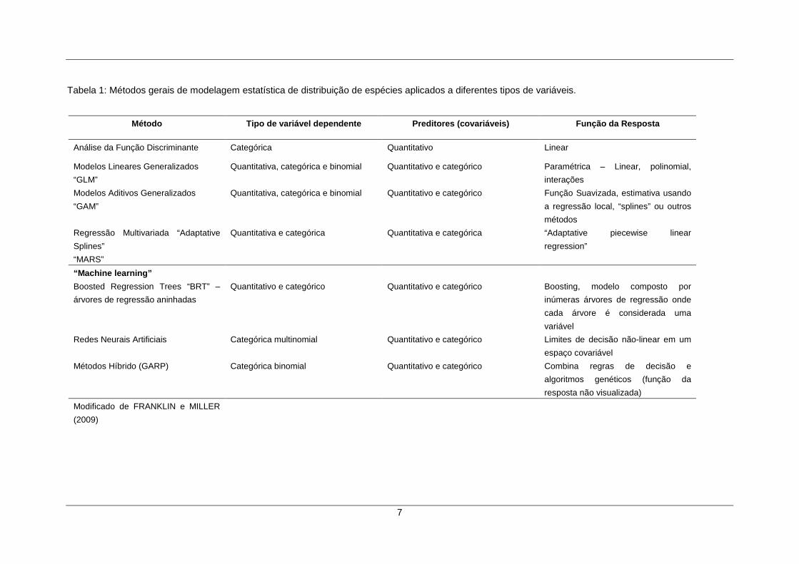
pesquisador em função do tipo de dados disponíveis. A Tabela 1 apresenta algumas
das metodologias mais utilizadas atualmente.
7
Tabela 1: Métodos gerais de modelagem estatística de distribuição de espécies aplicados a diferentes tipos de variáveis.
Método Tipo de variável dependente Preditores (cova riáveis) Função da Resposta
Análise da Função Discriminante Categórica Quantitativo Linear
Modelos Lineares Generalizados
“GLM”
Quantitativa, categórica e binomial Quantitativo e categórico Paramétrica – Linear, polinomial,
interações
Modelos Aditivos Generalizados
“GAM”
Quantitativa, categórica e binomial Quantitativo e categórico Função Suavizada, estimativa usando
a regressão local, “splines” ou outros
métodos
Regressão Multivariada “Adaptative
Splines”
“MARS”
Quantitativa e categórica Quantitativa e categórica “Adaptative piecewise linear
regression”
“Machine learning”
Boosted Regression Trees “BRT” –
árvores de regressão aninhadas
Quantitativo e categórico Quantitativo e categórico Boosting, modelo composto por
inúmeras árvores de regressão onde
cada árvore é considerada uma
variável
Redes Neurais Artificiais Categórica multinomial Quantitativo e categórico Limites de decisão não-linear em um
espaço covariável
Métodos Híbrido (GARP) Categórica binomial Quantitativo e categórico Combina regras de decisão e
algoritmos genéticos (função da
resposta não visualizada)
Modificado de FRANKLIN e MILLER
(2009)

8
Segundo Valavanis et al. (2008), os modelos a serem empregados dependem da
acurácia e do tipo de dado disponível. Basicamente, temos três tipos de dados que
podem ser usados pelo usuário, presença (1: presença), presença e ausência (1:
presença e 0: ausência) e dados contínuos (eg. abundância e densidade). Dados que
apresentam somente a presença são obtidos geralmente em bancos de dados de
coleções biológicas, considerando somente a ocorrência do registro na coleção. No
entanto, para dados de presença e ausência considera-se saber a ocorrência ou não
de um registro, sendo geralmente são advindos de coletas padronizadas. A seguir,
apresentamos uma revisão dos métodos de modelagem espacial mais utilizados
disponíveis na literatura. Estas metodologias foram divididas em modelos que usam
somente dados de presença e modelos que utilizam dados de presença, ausência e
dados contínuos.
1.1 MODELOS SOMENTE COM DADOS DE PRESENÇA
1.1.1 ENFA (Ecological Niche Factor Analysis)
A metodologia Ecological Niche Factor Analysis (ENFA) é utilizada para dados
somente de presença, normalmente dados de coleções biológicas. A comparação é
realizada com a distribuição estatística das variáveis geográficas em relação as
localidades onde a espécie é encontrada, como uma Análise dos Componentes
Principais, onde o algoritmo reúne os preditores com maior importância (HIRZEL et al.,
2006; VALAVANIS et al., 2008). No trabalho realizado por MaCleod et al. (2008) foi
verificado que modelagem ENFA é eficaz e pode ter performance melhor que modelos
GLM e GARP.
1.1.2 BIOCLIM
Foi um dos primeiros softwares usados para modelagem de distribuição de
espécies (BUSBY, 1986). No trabalho realizado por Busby (1986) foram utilizados
como preditores variáveis climáticas, obtidas por estações climatológicas, para a
predição de ocorrência de uma espécie de planta, Nothofagus cunninghamii (Hook)
Oerst. Esta metodologia consiste em ser um classificador que define a potencial
distribuição de uma espécie no espaço multidimensional definido pelos valores
máximos e mínimos identificados para todas as presenças (FRANKLIN e MILLER,
2009). O BIOCLIM é relacionado a teoria de nicho, onde o algoritmo procura por

9
delinear a área que melhor circunscreve as condições adequadas delimitadas pela
variáveis ambientais (VALAVANIS et al., 2004). No entanto, algumas deficiências
foram identificadas no modelo BIOCLIM, pois o modelo trata cada eixo climático
independentemente, o que pode levar a alguns casos de explicações ecológicas sem
sentido (BOOTH, 1990). A metodologia DOMAIN foi desenvolvida para corrigir estas
imperfeições.
1.1.3 DOMAIN
A metodologia de modelagem DOMAIN é um avanço em relação ao BIOCLIM,
pois este processo considera a potencial distribuição baseada em uma padronização
das ocorrências, calcula uma similaridade entre os pontos e apresenta um simples e
robusto método para modelagem de distribuição potencial de plantas e animais
(CARPENTER et al., 1993). Caracteriza-se por um método baseado em similaridade
que identifica novos locais considerando sua similaridade ambiental para locais de
ocorrência conhecida da espécie (VALAVANIS et al., 2004).
1.1.4 GARP
O Genetic Algorithm for Rule-Set Prediction (GARP) usa um algoritmo genético
que gera e seleciona uma população de regras que melhor predizem a distribuição de
uma espécie (STOCKWELL e PETERSON, 2002). O algoritmo GARP em comparação
com outros algoritmos constitui-se um bom método de modelagem espacial quando o
usuário tem em mãos pequenos grupos de dados tipicamente advindos de coleções
de museus (STOCKWELL e PETERSON, 2002). Uma aplicação do algoritmo GARP é
disponibilizada na internet através do Lifemapper (http://www.lifemapper.org), sendo
um atlas preditivo da biodiversidade biológica.
1.1.5 MAXENT
A metodologia de Máxima Entropia, conhecida como MAXENT, é um algoritmo
desenvolvido para análise de finanças e astronomia e se aplica a modelagem de
espécies com registros de somente presença (DUDÍK et al., 2007; PHILLIPS et al.,
2006). A máxima entropia é um princípio da teoria da informação que parte do
pressuposto que a probabilidade da distribuição de máxima entropia de uma espécie
(mais próxima da distribuição uniforme) decorrente de condicionantes conhecidos, é a

10
melhor aproximação de uma distribuição desconhecida (ELITH et al., 2011; FRANKLIN
e MILLER, 2009).
1.2 MODELOS COM DADOS DE PRESENÇA E AUSÊNCIA
1.2.1 Árvores de classificação e regressão CART
As árvores de classificação e árvores de regressão são metodologias ideais para a
análise de dados ecológicos complexos (DE’ATH e FABRICIUS, 2000) e esta
metodologia vem sendo desenvolvida nos últimos 25 anos (BREIMAN et al., 1984).
Além de ser uma metodologia em que o resultado final é facilmente interpretado, uma
das vantagens é a sua flexibilidade, pois este método pode usar variáveis não
lineares, podendo existir interações de alta ordem1 e valores faltantes (FRANKLIN;
MILLER, 2009).
Segundo a metodologia apresentada por De’ath e Fabricius (2000) para análise de
dados ecológicos, a variação da resposta é explicada pela repetida divisão dos dados
em grupos homogêneos, usando a combinação das variáveis que podem ser
categóricas e numéricas. Ao final, cada grupo é caracterizado pelo valor da variável
resposta, pelo número de observações no grupo e os valores das variáveis que os
definem.
1.2.2 Boosted regression Trees (BRT)
O metodologia Boosted Regression Trees (BRT) é flexível para o uso de
diferentes tipos de preditores (categóricos e contínuos) suportando valores faltantes e
lidando bem com outliers, respostas não lineares, além de não necessitar
transformações dos dados para o ajuste do modelo ( MOISEN e FRESCINO, 2002;
FRIEDMAN e MEULMAN, 2003; LEATHWICK et al., 2006, 2008; DE’ATH, 2007;
FRANKLIN e MILLER, 2009).
Os modelos BRT consistem na combinação de dois algoritmos: árvores de
regressão e boosting. As árvores de regressão foram descritas pela primeira vez por
Breiman (1984), seguido por De’ath e Fabricius (2000) e Hastie et al. (2008). A árvore
1 Interações de alta ordem ocorrem quando uma resposta, por exemplo a distribuição espacial de uma espécie, é afetada pela força da interação de duas ou mais variáveis (BILLICK; CASE, 1994).

11
de regressão é construída por várias divisões dos dados objetivando a partição da
resposta em grupos homogêneos (DE’ATH e FABRICIUS, 2000).
A técnica de boosting consiste na mistura dos resultados de múltiplos modelos,
neste caso árvores de regressão, baseando-se no princípio geral de que achando
muitas respostas razoáveis pode ser mais fácil do que encontrar uma única resposta
altamente precisa para uma predição (SCHAPIRE, 2003). Boosting é uma otimização
numérica que objetiva a redução dos erros por adicionar a cada passo do algoritmo
uma nova árvore de regressão (ELITH et al., 2008). Dessa maneira, centenas de
árvores de regressão são construídas e o modelo BRT consiste em uma combinação
linear de várias árvores, que pode ser visto como um modelo de regressão onde cada
termo é uma árvore (ELITH e LEATHWICK, 2012).
1.2.3 Multivariate Adaptative Regression Splines (M ARS)
A metodologia Multivariate Adaptative Regression Splines (MARS) tem sido pouco
usada em modelos de distribuição espacial, sendo mais aplicada em áreas como a
química, engenharia, medicina e epidemiologia (FRANKLIN e MILLER, 2009).
Segundo Hastie et al. (2008), MARS consiste em ser um método adaptativo para
regressão, e ele é indicado para problemas de grandes dimensões, como por exemplo
grupos de dados muito grandes. Ainda segundo Hastie et al. (2008) ele pode ser visto
como uma generalização de uma regressão linear particionada, ou uma modificação
da metodologia CART. Segundo Franklin e Miller (2009) essa metodologia não é
adequada para dados binomiais (presença e ausência), no entanto Leatwick et al.
(2005) conseguiu contornar essa limitação alterando as funções básicas do algoritmo
computado no software R.
1.2.4 Modelos Lineares Generalizados (GLM)
Como a grande parte das relações ecológicas não são lineares, modelos lineares
generalizados ou Generalized Linear Models (GLMs) são amplamente utilizados. Os
GLMs oferecem vantagem pois esta metodologia permite transformar a variável
resposta em padrão não linear (MILLER e FRANKLIN, 2002; VENABLES e RIPLEY,
2002). A transformação da variável resposta, por exemplo, a abundância de uma
espécie, é realizada pela função link, que pode assumir diferentes famílias
dependendo das estruturas dos erros, (e.g. Poisson para dados de contagem) ou
outras formas de erro (Crawley, 2005). Na abordagem de modelagem utilizando-se

12
GLMs a característica da variável resposta pode assumir diferentes padrões de
distribuição como Poisson, Gaussiano ou Binomial (regressão logística). Ainda,
respostas não lineares podem ser obtidas através da incorporação de valores de Y
elevados ao quadrado e ao cubo, emulando respostas polinomiais, mas com a
desvantagem da adição de graus de liberdade.
Umas das primeiras aplicações de GLMs para a modelagem de distribuição
espacial foi apresentada por Nicholls (1989). Neste trabalho o autor ajustou modelos
de regressão logística para predição de ocorrência espacial para três espécies do
gênero Eucalyptus, apresentando também metodologias para a realização de
diagnóstico do modelo considerando o uso dos resíduos da regressão. Dentre as
vantagens do GLM destaca-se a fácil compreensão dos resultados do modelo final,
assim como a reprodutibilidade do modelo de regressão através dos coeficientes
estimados para cada variável selecionada.
1.2.5 Regressão logística
Os modelo de regressão logística, da família GLM, permite realizar a modelagem
de uma variável em função de preditores de natureza binária, assumindo valores de 0
ou 1 (BEWICK et al, 2005). Esta técnica de modelagem vem sendo aplicada para
prever a distribuição de espécies em uma matriz de paisagem com inúmeras
aplicações para o gerenciamento ambiental (PEARCE e FERRIER, 2000). O uso de
modelos de regressão logística vem sendo empregados na predição de ocorrência em
peixes (PEARCE e FERRIER, 2000; PORTER, 2000; ALVES e FONTOURA, 2009;
BARRADAS et al. 2012), anfíbios (KOLOZSVARY e SWIHART, 1999), aves
(SYARTINILIA, 2008), invertebrados (BARBOSA e MELO, 2009), dentre outros grupos
taxonômicos.
1.2.6 Modelos Aditivos Generalizados (GAM)
Os modelos aditivos generalizados (ou a sigla em inglês, GAM) se tornaram muito
populares desde a publicação do trabalho de Wahba (1990). A metodologia GAM
(HASTIE e TIBSHIRANI 1986; HASTIE e TIBSHIRANI, 1990) é um modelo linear
generalizado com um preditor linear envolvendo a soma das funções suavizadoras
(não lineares) das covariáveis. Esta metodologia caracteriza-se em ser uma
abordagem flexível para identificar e descrever relações não-lineares entre preditores
e a variável resposta através de funções suavisadoras (YEE AND MITCHELL, 1991).

13
O trabalho realizado por Borchers et al. (1997) foi um dos primeiros trabalhos
empregando o uso da metologia GAM na modelagem de distribuição de espécies.
Neste estudo foram ajustados modelos GAM para a distribuição de ovos de duas
espécies de “mackerel” (Scomber scombrus e Trachurus trachurus), no atlântico norte.
Apesar da vantagem deste método ser eficiente na identificação e descrição de
respostas não lineares, os autores citam a dificuldade na seleção do modelo
considerando o tipo de função suavisadora, além da seleção das variáveis a compor o
modelo.
1.2.7 Redes Neurais Artificiais (RNA)
A metodologia de Redes Neurais Artificiais (em inglês: Artificial Neural Networks,
ANN) consiste em uma ferramenta eficiente para predição de ocorrência de espécies.
Em ecossistemas complexos, é comum que as variáveis mensuradas não apresentem
um padrão linear. Nestes casos, as RNAs vêm sendo usadas e comparadas as outras
metodologias (regressão linear e logística) se mostrando mais flexível e robusta
quando as variáveis apresentam padrões irregulares (LEK et al., 1996; OLDEN e
JACKSON, 2001).
As RNAs foram desenvolvidas para pesquisa de modelos de aprendizado no
cérebro humano, sendo considerada uma técnica de machine learning, ou
aprendizagem de máquina. Métodos considerados machine learning, ou de
aprendizagem de máquina, consistem em algoritmos que são usados para aprender
uma função de mapeamento ou conjunto de regras de classificação diretamente a
partir de um grupo de dados de treino (BREIMAN, 2001; GAHEGAN, 2003). Uma
aplicação simples de metodologias de aprendizado de máquina são utilizadas em
filtros de correios eletrônicos, onde o algoritmo aprende a selecionar mensagens spam
ou mensagem sem perigo para computadores. As RNAs são amplamente empregadas
em diversas áreas do conhecimento, como no sensoriamento remoto para
classificação de imagens, em economia e biologia (GERMAN e GAHEGAN, 1996;
KHAN et al., 2001; ZHANG et al., 1998).

14
1.3 CONSIDERAÇÕES SOBRE A ESCOLHA DA METODOLOGIA DE MODELAGEM
Existe atualmente diversas técnicas desenvolvidas para a modelagem de
distribuição de espécies. Dentre as diferentes técnicas disponíveis, algumas são mais
exigentes (e.g., modelos lineares e regressão logística), exigindo normalidade dos
dados e sendo muito sensíveis a outliers. No entanto, algumas metodologias são mais
flexíveis, aceitando dados faltantes, não sendo sensíveis a outliers e aceitando
variáveis categóricas e contínuas (e.g., BRT e RNA). Portanto, para escolha de um
modelo estatístico o usuário deve levar em consideração a qualidade do seus dados e
se a metodologia é adequada aos dados disponíveis.
Em relação a dados oriundos de coleções biológicas, técnicas de modelagem
espacial que aceitem somente dados de presença são as indicadas, como BIOCLIM e
MAXENT. Essas metodologias foram desenvolvidas com esse propósito, onde o
usuário tem somente a informação da ocorrência e não tem a informação da ausência
confirmada. Portanto, os dados somente de presença de uma espécie podem ter
informação útil para a modelagem espacial, mas podem haver limitações quanto as
conclusões obtidas na avaliação do modelo.
Por outro lado, algumas metodologias exigem maior controle na amostragem e
informações de presença e ausência são necessárias, caso do modelos lineares,
regressão logística, árvores de classificação (CART) e GLMs. Nestes casos, para
evitar ruídos nos resultados sugere-se que a metodologia de amostragem seja
padronizada ou apresente termos no modelo para o controle desta variação. Por
exemplo, no trabalho realizado por Leathwick et al. (2006) em amostragens de peixes
demersais, os arrastos de fundo não foram padronizados, variando em distância e
velocidade do arrasto. Neste caso, o problema foi corrigido pela inclusão de duas
variáveis no modelo, velocidade do arrasto e distância do arrasto.
A escala do estudo deve ser levada em consideração para a escolha das variáveis
disponíveis para os modelos. Para o desenvolvimento de modelos de distribuição
espacial, usa-se camadas de variáveis ambientais disponíveis para o usuário e as
mais comuns são: altitude, declividade, vegetação, tipo de solo, área de bacia, dentre
outras. Algumas variáveis disponíveis apresentam-se em escalas de 30x30m à
90x90m, no caso de imagens do satélite LANDSAT. Portanto, para o desenvolvimento
de modelos de distribuição espacial as variáveis obtidas em micro hábitats dificilmente

15
podem ser interpoladas para a obtenção de uma camada de variável para
posteriormente se produzir um mapa de distribuição.
A modelagem da distribuição espacial de espécies, segundo Austin (2002), deve-
se considerar três componentes básicos: um modelo ecológico considerando a teoria
ecológica a ser testada, os dados coletados disponíveis e o modelo estatístico a ser
empregado. Considerando que a combinação destes três aspectos pode apresentar
diferentes cenários, uma boa alternativa é balizar a escolha segundo o estudo
realizado por Ferrier et al. (2006) onde foram comparados diferentes modelos e
diferentes tipos de dados para testar a eficiência de cada metodologia. No entanto,
Guisan e Thuiller (2005) enfatizam que a metodologia de modelagem nunca substituirá
a qualidade da matriz de dados disponível.

16
2 O LAGO GUAÍBA
O lago Guaíba localizado na bacia hidrográfica de mesmo nome, banha a cidade
de Porto Alegre, no Estado do Rio Grande do Sul (Brasil), sendo abastecido por oito
sub - bacias do centro e nordeste do Rio Grande do Sul, em uma área de
aproximadamente 84.763,5 km2 (NICOLODI, 2007). Apresenta um volume de
aproximadamente 1,5 bilhões de metros cúbicos (SALOMONI e TORGAN, 2008) com
área de cerca de 500 km2, com aproximadamente 50 km de comprimento e 19 km de
largura no ponto mais largo. Constitui-se como um enxutório dos Rios Jacuí, Gravataí,
Caí e Sinos (Fig. 3). A profundidade do canal de navegação é de aproximadamente 7
m, embora a profundidade média do lago seja de apenas 2,5 m. A área mais profunda,
atinge aproximadamente 60 m em ponto isolado ao sul do lago, perto da sua foz na
Laguna dos Patos.
Figura 3: Localização do Lago Guaíba.
As margens do Lago consistem em uma sequência de compartimentos,
localmente denominadas por sacos, separados geralmente por penínsulas de origem

17
geológica granítica (MANSUR et al., 2003) ou bancos de areia devidos à circulação de
água decorrente do regime de ventos. As margens do Lago Guaíba consistem
geralmente de praias arenosas com grandes áreas vegetadas.
Quanto a diversidade de tipos de hábitat, o lago Guaíba apresenta diferentes
características influenciadas por variáveis bióticas e abióticas. Dentre os elementos
bióticos, conferindo heterogeneidade espacial ao lago, podemos destacar a vegetação
aquática, representada principalmente pelo junco, Scirpus californicus (CA Mey.)
Steud., bem como outras macrófitas: Pistia stratiotes L. e Eichornea azurea (Sw.)
Kunth. Quanto as variáveis abióticas, que apresentam um gradiente ambiental no lago
Guaíba, pode-se destacar o sedimento de fundo, banhados associados, parcéis
rochosos, foz de rios e canais, diferentes intensidades de circulação da água,
profundidade e qualidade da água. A figura 4 ilustra a variação da velocidade da
corrente no Lago Guaíba em cenários de estiagem e de chuvas. Esta velocidade de
corrente influencia principalmente as características do sedimento de fundo em
sinergismo com a profundidade.

18
Figura 4: Percentual de velocidades menores que 5,0 cm/s, 30 dias de simulação pelo Modelo Hidrodinâmico 2DH SisBahia em período de estiagem (janeiro) e chuvas (julho). Modificado de (LERSCH et al., 2013)
O Lago Guaíba é afetado pelo regime hídrico em diferentes épocas do ano e pelos
ventos, podendo ser também afetado por uma combinação de ambos (KNIPLING,
2002). O vento do quadrante sul pode represar suas águas e chuvas nas cabeceiras
de seus tributários podem aumentar seu nível. Durante as cheias, o nível do lago pode
atingir a cota de 4 m em algumas regiões, podendo conectar-se com as zonas úmidas
adjacentes (NICOLODI et al., 2011). O vento também exerce importante influência na
qualidade da água pela geração de ondas que provocam ressuspensão de sedimento
fino no lago. Segundo Nicolodi (2007), a profundidade máxima do lago em que o vento
pode causar turbulência no fundo e gerar ressuspensão de sedimento fino é de 1,9 m.
A qualidade da água no Lago Guaíba varia em um gradiente de distância de
fontes poluidoras, sendo mais intensa com a proximidade aos centros urbanos. A
porção norte do Lago, junto ao Delta do Jacuí, apresenta a pior qualidade de água,
segundo o levantamento realizado por Bendati et al. (2000). Nesta localização são
19
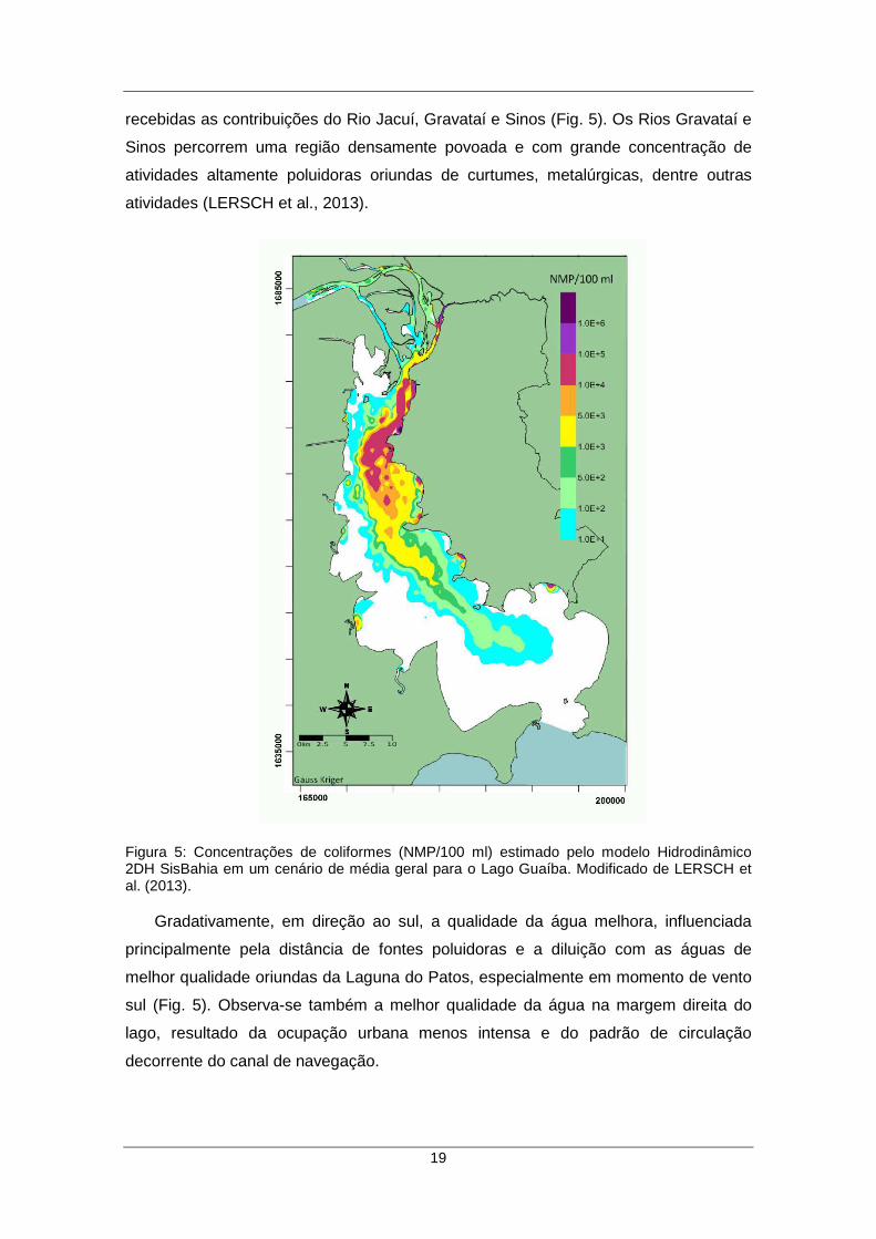
recebidas as contribuições do Rio Jacuí, Gravataí e Sinos (Fig. 5). Os Rios Gravataí e
Sinos percorrem uma região densamente povoada e com grande concentração de
atividades altamente poluidoras oriundas de curtumes, metalúrgicas, dentre outras
atividades (LERSCH et al., 2013).
Figura 5: Concentrações de coliformes (NMP/100 ml) estimado pelo modelo Hidrodinâmico 2DH SisBahia em um cenário de média geral para o Lago Guaíba. Modificado de LERSCH et al. (2013).
Gradativamente, em direção ao sul, a qualidade da água melhora, influenciada
principalmente pela distância de fontes poluidoras e a diluição com as águas de
melhor qualidade oriundas da Laguna do Patos, especialmente em momento de vento
sul (Fig. 5). Observa-se também a melhor qualidade da água na margem direita do
lago, resultado da ocupação urbana menos intensa e do padrão de circulação
decorrente do canal de navegação.
20
3 ORGANISMOS AQUÁTICOS ESTUDADOS
Foram escolhidas para a modelagem da distribuição espacial no lago Guaíba
quatro espécies: o bivalve Corbicula fluminea (Müller, 1974); e três espécies de
Siluriformes, Pimelodus pintado Azpeculieta, Lundberg & Loureiro, 2008;
Parapimelodus nigribarbis Boulenger (1889) e Loricariichtys anus (Valencines, 1835).
As espécies foram escolhidas com base em sua abundância nas amostragens,
importância ecológica e para a pesca.
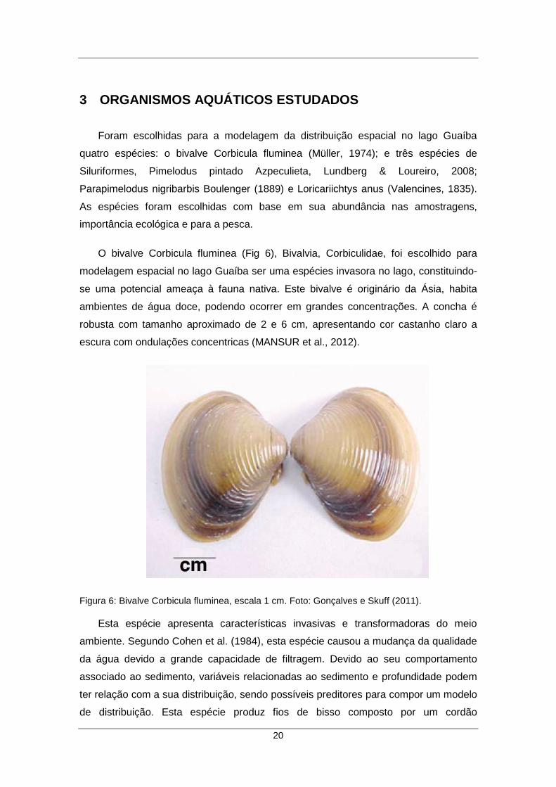
O bivalve Corbicula fluminea (Fig 6), Bivalvia, Corbiculidae, foi escolhido para
modelagem espacial no lago Guaíba ser uma espécies invasora no lago, constituindo-
se uma potencial ameaça à fauna nativa. Este bivalve é originário da Ásia, habita
ambientes de água doce, podendo ocorrer em grandes concentrações. A concha é
robusta com tamanho aproximado de 2 e 6 cm, apresentando cor castanho claro a
escura com ondulações concentricas (MANSUR et al., 2012).
Figura 6: Bivalve Corbicula fluminea, escala 1 cm. Foto: Gonçalves e Skuff (2011).
Esta espécie apresenta características invasivas e transformadoras do meio
ambiente. Segundo Cohen et al. (1984), esta espécie causou a mudança da qualidade
da água devido a grande capacidade de filtragem. Devido ao seu comportamento
associado ao sedimento, variáveis relacionadas ao sedimento e profundidade podem
ter relação com a sua distribuição, sendo possíveis preditores para compor um modelo
de distribuição. Esta espécie produz fios de bisso composto por um cordão

21
mucilaginoso elástico, presente apenas na fase de recrutamento. Segundo Prezant e
Chalermwat (1984), a formação desta estrutura é estimulada pela correnteza,
auxiliando na dispersão. No entanto, segundo Mansur et al. (2012) cita que este fio ou
cordão mucilaginoso funcionaria como uma âncora, aglutinando areia e evitando o
arraste do molusco pela correnteza.
A espécie P. pintado (Siluriformes, Pimelodidae) (Fig. 7) conhecida como pintado,
foi escolhida para fins de modelagem por se constituir umas das espécies mais
abundandantes nas amostragens realizadas. Esta espécie apresenta corpo fusiforme
com coloração cinza no dorso e laterais, branco amarelado no ventre e manchas
pretas dispostas sem padrão pelo corpo (BENVENUTI e MORESCO, 2005,
AZPELICUETA et al. 2008). Espécies deste gênero podem apresentar comportamento
onívoro possuindo grande plasticidade de hábitos alimentares, conferindo capacidade
de adaptação frente a impactos ambientais (LUZ-AGOSTINHO et al., 2006; RAMOS et
al., 2011). Espécies deste gênero podem ocorrer em reservatórios, rios e lagos,
usando estes hábitats para forrageamento e crescimento, quando entra em período
reprodutivo migra para ambientes lóticos (DEI TOS et al., 2002; LUZ-AGOSTINHO et
al., 2006; MAIA et al., 2007; AZPELICUETA et al. 2008).
Figura 7: Pimelodus pintado. A, Holótipo fresco; B, Parátipo jovem fixado. Foto: M. Loureiro. Modificado de Azpelicueta et al. (2008).
A espécie Parapimelodus nigribarbis (Fig. 8) foi escolhida para fins de modelagem
espacial devido a sua abundância nas amostragens ocorridas na realização do projeto.

22
Esta espécie apresenta coloração cinza-prateada no dorso com o ventre branco ou
amarelado, sendo levemente comprimido dorsoventralmente (LUCENA et al., 1992).
Esta espécie costuma ocorrer em grandes cardumes se alimentando principalmente
de plâncton, além de insetos (MORESCO e BENVENUTI, 2005). No trabalho realizado
por Dufech e Fialho (2009) foi verificada maior captura com redes de espera quando
comparado com arrasto de praia, sugerindo uma tendência da espécie em ocorrer na
zona limnética. A captura somente em região limnética também foi observada por
Artioli et al. (2009). No entanto, no trabalho realizado por Lucena et al. (1992) foi
relatada a captura em grandes quantidades junto as margens. Preditores como
profundidade e distância da margem podem ser importantes para a ocorrência da
espécie.
Figura 8: Parapimelodus nigribarbis. Foto: Cláudio Dias Timm (Disponível em <www.fishbase.org> acesso em: 10/01/2014).
A espécie Loricariichthys anus (Siluriformes, Loricariidade), é conhecida
popularmente como viola ou cascudo-viola (Fig. 7). Esta espécie foi escolhida por se
constituir uma espécie de interesse para a pesca (PETRY e SCHULZ, 2000).
apresenta corpo deprimido, cor parda-amarelada clara e cabeça pontiaguda, com 34-
35 placas ósseas (BEMVENUTI e MORESCO, 2005). Esta espécie apresenta hábitos
diurnos relacionados ao forrageio com hábito alimentar omnívoro, segundo estudo
realizado por Petry e Schulz (2000). No estudo realizado por Dufech et al. (2009) foi
comparada uma lagoa isolada do parque Estadual de Itapuã e uma praia com fundo
arenoso no lago Guaíba. Neste estudo foi observado que L. anus teve abundâncias 6
vezes maior em praia com fundo arenoso do que na lagoa isolada, sugerindo uma
preferência por este tipo de hábitat. Esta espécie ocorre em diferentes situações no

23
lago Guaíba, conforme estudos realizados na região (MARQUES et al., 2007;
FLORES-LOPES e CETRA, 2010; SACCOL-PEREIRA e FIALHO, 2010). A ocorrência
desta espécie pode estar relacionada a complexidade ambiental e associada a fluxos
de água moderados, podendo a distância da margem e dinâmica do fluxo da água
serem variáveis importantes para a seleção de habita.
Figura 6: Loricariichthys anus. Foto: Cláudio Dias Timm (Disponível em <www.fishbase.org> acesso em: 10/01/2014).

24
4 JUSTIFICATIVA
Apesar do amplo conhecimento sobre as espécies de peixes presentes no Lago
Guaíba (MALABARBA, 1989; REIS, et al., 2003) e assim como os invertebrados
(FOCHT e VEITENHEIMER-MENDES, 2001; MANSUR e PEREIRA, 2006; MANSUR
et al., 2012) presentes no Lago Guaíba, existe pouco conhecimento técnico-científico a
cerca dos fatores que influenciam na distribuição da fauna aquática em pequena
escala no Lago Guaíba, bem como o desenvolvimento de modelos de distribuição
espacial para a ocorrência destas. Além disso, a aplicação de metodologias de
Sistema de Informação Geográfica (SIG) combinadas com o estudo da adequabilidade
de hábitat em ecossistemas lacustres ainda é escassa na literatura acadêmica.
Portanto, os resultados deste trabalho iniciam uma linha de trabalho da modelagem de
ocupação de hábitat invertebrados e peixes no lago Guaíba bem como apresenta os
primeiros dados referentes a modelagem da distribuição de espécies aplicada à
ecossistemas aquáticos lacustres regionais. Os resultados deste trabalho também
podem auxiliar órgãos de fiscalização ambiental na conservação dos ecossistemas
aquáticos do lago Guaíba e na tomada de decisão a cerca de empreendimentos que
possam impactar o Lago Guaíba e ecossistemas associados.

25
5 OBJETIVOS
5.1 OBJETIVO GERAL
Modelar a distribuição espacial e a abundância de Corbicula fluminea, Pimelodus
pintado, Parapimelodus nigribarbis e Loricariichthys anus no Lago Guaíba em relação
a diferentes variáveis ambientais.
5.2 OBJETIVOS ESPECÍFICOS
− Identificar, para de C. fluminea, P. pintado, P. nigribarbis e L. anus, as
variáveis ambientais com poder preditivo para fins de modelagem de distribuição;
− Produzir um conjunto de mapas com variáveis ambientais do Lago Guaíba,
considerando aspectos de qualidade de água, circulação, fisionomia de fundo e
características do sedimento;
− Ajustar modelos estatísticos de distribuição para cada uma das espécies com
base nas variáveis ambientais selecionadas;
− Produzir mapas da predição das abundâncias das espécies selecionadas
através da aplicação dos modelos estatísticos ajustados.

26
CAPÍTULO 1: Spatial distribution modeling of the in vasive clam in Guaíba Lake, Southern Brazil
Artigo a ser submetido para a revista “Aquatic Ecol ogy”

27
Spatial distribution modeling of the invasive clam Corbicula fluminea in Guaíba 1
Lake, Southern Brazil 2
Thiago Cesar Lima Silveira1*; Irene Martins2; Thais Paz Alves1; Nelson Ferreira 3
Fontoura1 4
1. Pontifícia Universidade Católica do Rio Grande do Sul, Departamento de 5
Biodiversidade e Ecologia, Laboratório de Ecologia Aquática, Avenida Ipiranga 6681, 6
CEP 90.619-900, Porto Alegre, RS, Brazil. 7
2. School of Ocean Sciences, Bangor University, Menai Bridge, Anglesey, LL59 8
5AB, UK 9
*Corresponding author: [email protected] 10
Abstract 11
The aim of this study was to analyse the relationships of the clam Corbicula 12
fluminea with environmental predictors in a lake in the southern Neotropical region of 13
Brazil to predict patterns of habitat suitability. The analyses were carried out using 14
Generalized Additive Models (GAM). We used a data set comprising 54 observations 15
and the predictors evaluated were depth, organic matter of sediment, average 16
granulometry, percentage of sand, Shannon diversity of sand grains size, distance from 17
margins, and distance from rivers, Average water speed and the amount of 18
thermotolerant bacteria. The best model had depth and diversity of sand grains as 19
explanatory variables. Our results indicate that C. fluminea tends to occur mainly in 20
sandy sediments with low organic matter content, neither too deep (1 m) nor by the 21
shore. Our results showed the spatial distribution modelling of C. fluminea in an 22
invaded environment contributing to the knowledge of species autecology and a better 23
understanding of ecological relationships in Guaíba Lake. 24
Key words: Corbiculidae, habitat suitability modelling, generalized additive model, 25
exotic species; South America 26
27

28
Introduction 28
Spatial Distribution Models (SDMs) use multiple environmental variables to predict 29
the presence or the abundance of a given species in any area of interest, acting as a 30
mathematical tool to depict the multidimensional niche of species sensu Hutchinson 31
(1957). The SDMs are methods to estimate the probability of a species presence or 32
presumed abundance in relation to a given number of environmental predictors, with 33
application in conservation, wildlife management, environmental impacts evaluation 34
and predicting scenarios of exotic species invasions (Franklin and Miller, 2009; Guisan 35
and Thuiller, 2005). 36
Modeling habitat suitability and distributional patterns are important goals in 37
Ecology due to their application in conservation strategies (Franklin and Miller, 2009). 38
Major difficulties are related to the unavailability of detailed environmental layers, 39
especially for aquatic environments. Although, successful examples of distributional 40
inference patterns with relative few predictors have been described for river freshwater 41
fish by Alves and Fontoura (2009) and Barradas et al. (2012). However, spatial 42
distribution models for freshwater species in lakes are still scarce. In South America, a 43
recent study of Guimarães et al. (2014) analysed the effects of connectivity in fish 44
richness in coastal lakes. 45
Introduction of exotic species in freshwater ecosystems threatens diversity; 46
changes ecosystem natural cycles and causes the extinction of native biota (Lodge et 47
al., 1998). In the past 30 years, the Neotropical region (including southern Florida, 48
Mexican lowlands, South and Central America, and the Caribbean islands) suffered the 49
introduction of at least two mussel species, causing negative environmental and 50
economic impacts (Darrigran, 2002). One of these species is Corbicula fluminea 51
(Müller, 1774). 52
Corbicula fluminea is an Asiatic edible clam well known for their invasive success 53
(Cohen et al., 1984; Araujo et al., 1993; Cataldo and Boltovsky, 1998). The species has 54
physiological, environmental and behavioural adaptations to living in lotic environments 55
(Britton and Morton 1979) although its occurrence in lakes is also reported (Cenzano 56
and Würdig, 2006). The introduction of C. fluminea in inland waters in South America 57
occurred by ballast water transport and discharge, with the first record in Rio da Prata – 58
Uruguay, and has been reported since 1970 (Veitenheimer-Mendes, 1981; Focht and 59
Veitenheimer-Mendes, 2001). The species is now widespread in Brazilian freshwaters 60
basins (Rodrigues and Pires-Junior, 2007). 61

29
Corbicula fluminea has an aggressive invasive behaviour, being able to colonize 62
diverse habitats, competing with native species, as Anodontites trapesialis (Lamarck, 63
1819) and Leila blainvilliana (Lea, 1834), due to the high rate of reproduction and 64
filtering (Gardner et al., 1976; Phelps, 1994). Large colonies can improve the water 65
transparency by filtration, change algae and macrophyte production and influence all 66
the ecosystem dynamics (Phelps, 1994; Sousa et al. 2008). Additionally, the invasive 67
ability of C. fluminea is enhanced by flotation strategies as a mean of dispersal, a 68
behaviour that is triggered by the water flowing stimuli (Prezant and Chalermwat, 69
1984). 70
According to McMahon (1981), in environments with lentic dynamics, C. fluminea is 71
restricted to shallow and oxygenated margins. Is expected that C. fluminea occurs in 72
similar habitats. Nevertheless, despite the environmental conditions of C. 73
fluminea occurrence being already described in the literature, studies aiming to model 74
the habitat suitability to this species still scarce in lentic environments. 75
In this regard, our aims were to model the habitat suitability of C. fluminea with a 76
method capable to identify the ecological relationships of this species in Guaíba Lake, 77
while also producing a map of predicted abundance that could be used in conservation 78
strategies. 79
Material and Methods 80
Study Area 81
The Guaíba Lake (Fig.1) is located in Southern Brazil beside the city of Porto 82
Alegre, presenting approximately 500 km2, with about 50 km in length and 19 km in 83
width in the widest site, with a central channel 5-6 m deep used by commercial ships. A 84
deeper area, achieving 60 m is located at the south of the lake, near its mouth with the 85
Patos lagoon. The margins consist of a sequence of bays, separated by sandy or rocky 86
peninsulas. The shores of Guaíba Lake generally consist of sandy beaches with large 87
areas of marshes, where Scirpus californicus (C.A. Mey.) Steud. is the most abundant 88
species. 89
The water level of Guaíba Lake depends mainly on the rainfall regime and winds, 90
and it is not under tidal influence. During floods, the lake level can reach the quota of 4 91
m and in some regions it can connect to wetlands. Also, south winds strongly 92
influences the water level, which may causes water impoundment and reversed flows 93
when blowing (Nicolodi et al., 2011). The main rivers (Jacuí, Caí, Sinos and Gravataí) 94

30
form a deltaic area; with several muddy islands in the northern limit of the lake, carrying 95
sediments and also considerable amounts of organic pollution. During the year, the 96
water discharge suffers strong alterations, with mean water flow of 1150 m3/s, but 97
attaining 355 m3/s in the dry season and the mean water flow is 1150 m3/s (Lersch et 98
al., 2013). 99
100
101
Figure 1: Guaíba Lake, southern Brazil. The black dots indicate the sampling sites. 102
Sampling methods 103
Samplings were performed from February 2011 to March 2013, in 54 points 104
distributed over the lake area (Fig. 1) sampled one time. At each sampling site we 105
obtained eleven subsamples with an Ekman dredge (225 cm2), 10 sub samples for C. 106
fluminea and one sample was intended for granulometric analysis. Sediment 107
subsamples were washed with a sieve (300 µm) and the captured clams were fixed in 108
a 10% formaldehyde solution. Species abundance for modelling was the sum of all the 109
ten sub samples (2250 cm²) at each sampling point. 110

31
Environmental Predictors 111
We investigated the relationships between C. fluminea abundance and nine 112
environmental predictors (Tab. 1). At each sampling point Depth (m) was measured 113
with a manual probe corrected by the annual mean readings from 2001 to 2011 of 114
Praça da Harmonia Scale due to the depth variation caused by the rainfall along the 115
year and winds. Sediment samples were transported to the laboratory, chilled on ice 116
and stored at -18o C until analysis. Sediment subsamples were dried and classified 117
through sieves with meshes sizes of 2000 µm; 1000 µm; 500 µm; 250 µm; 125 µm and 118
63 µm. The average granulometry (AvGran; µm) was calculated by a weighted average 119
corrected by the amount of sediment retained in each sieve of sediment classification. 120
Percentage of sand (PcSand; %) at each sampling point was estimated by dividing the 121
sediment retained above the 63µ sieve by the total dry sample weight (x100). To 122
determine organic matter content (OMC; %) 50 gr of dried sediment was burned 123
through 6 hours in the oven furnace at 550o C and the OMC was determined by weight 124
difference after the carbon oxidation. Also, we calculated the Shannon Diversity index 125
of grain sizes in the sample, becoming a metric of granulometry heterogeneity 126
(Het.gran). To obtain the Het.gran we considered each sediment classes as “species” 127
and the rounded value in grams as the abundances in each sediment class. 128
The environmental predictor distance from the nearest margin (D.marg) consisted 129
in the distance in meters, as well as the distance from the nearest tributaries (rivers, 130
streams, reaches, artificial channels; D.river). We identified the existence of 42 small 131
reaches and those were confirmed by using high resolution images on Quantum GIS 132
2.2 (QGIS Development Team, 2014), through the plugin Oppen Layers 1.3.1 133
(Sourcepole, 2014) which uses Google Maps® imagery. This search was carried out to 134
map all small water bodies that were not mapped by Hasenack and Weber (2010). 135
The predictor average water speed (Speed.Av) consists in the average percentage 136
of water speeds lesser than 5 cm/s. This average consists in a mean values modeled 137
by the Hydrodynamical model 2DH according to Lersch et al. (2013) considering the 138
dry (January) and wet (July) scenarios. Modeled counts of thermotolerant bacteria 139
were also used in the lake as Most Probable Number (MPN/100ml) by the 140
Hydrodynamical model 2DH consisting in a mean scenario considering the mean 141
annual flow (Lersch et al., 2013). 142
143

32
Table 1: Environmental predictors used in the analyses to predict Cobicula fluminea abundance 144 in Guaíba Lake, southern Brazil. 145
Variable Average (range)
Depth 2.55 m (0.7-6.2 m )
Averaged sand grain size (Av.gran) 0,45 µm (0.17 – 1.21 µm)
Percentage of sand (Pc.sand) 91.7 % (50.11 – 100 %)
Organic mater content (OM) 4.05 % (0.24 – 14.86 %)
Distance from the nearest margin (D.marg) 1009,6 m (0 – 4243 m)
Distance from the nearest channel (D.channel) 2939.58 m (0 – 9991,03 m)
Shannon Diversity index for granulometry (Het.gran) 1.02 (0.51 – 1.54)
Thermotholerant bacteria - Most probable number (MPN) 33858.17 (1.0e+1 – 1.0e+6 NMP/100 ml)
Average percentage of speeds lower than 5 cm/s (Speed.Av) 71.1% (1-100 %)
146
Were generated an environmental map concerning the distance from the nearest 147
margin (D.marg) and the distance from the nearest tributaries (D.river; rivers, streams, 148
reaches, artificial channels). Also, the environmental layers were obtained by 149
interpolating our observations by ordinary Kriging (supplementary material), except for 150
distance from margins and distance from channel. In order to increase the data for 151
interpolations we aggregated to our 54 measurements 177 points from the 152
Sedimentation Project of Guaíba Lake Complex report (CECO UFRGS and DMAE, 153
1999). 154
Statistical Analysis 155
First, we investigated the collinearity between the predictors by Variance Inflation 156
Factor (VIF) method (Dormann et al., 2013; Montgomery and Peck, 1982; Stine, 1995; 157
Wisz et al., 2013). For niche modelling of C. fluminea we used Generalized Additive 158
Models (GAM). We used data distribution family “Poisson” and carried out 159
transformations to handle with the heteroscedasticity. We selected the best model by 160
forward selection according to Zuur et al. (2009). We fit one model to each predictor 161
and kept the model with the lowest Unbiased Risk Estimator (UBRE) and all predictors 162
with p-value less than 0.05. Also, we evaluated the prediction of the selected model to 163
a new data set from Araçá Lagoon (Gama, 2004), linked to the Patos Lagoon system. 164

33
The variable importance was analyzed by the correlation of two models: one model 165
with the real data, and the other model with the values of the target variable randomly 166
shuffled. If the two models a have high correlation, the target variable is not important. 167
In the other hand, if they do not correlate, then the target variable is important. The 168
values were calculated as mean of 5 randomizations, expressed as 1- correlation 169
between the original model and the shuffled model, giving higher scores to more 170
important variables. This approach is similar to the method used in biomod (Thuiller et 171
al., 2014) and random forests (Liaw and Wiener, 2002). 172
We verified that the interpolated predictors could introduce bias in the prediction 173
map, because of the observed values do not correspond exactly to the values obtained 174
in the same location in the interpolated surfaces. In order to correct this we fitted 175
another empirical model (GAM) in order to correct the range (nested GAM). We used 176
the observed densities as response and the predicted values extracted from the map 177
as predictor. The fitted GAM was used to correct the range in the prediction map. 178
We carried out GAM under the RStudio 0.98.501 software (RStudio, 2014), an 179
integrated development environment for R software 3.0.3 (R Core Team, 2014) with 180
the functions of “mgcv” library (Wood, 2001). The interpolations were performed with 181
the package “gstat” (Pebesma, 2014) and “automap” (Hiemstra et al., 2009). The 182
prediction map and the map processing were performed in RStudio with the functions 183
of package “raster” (Hijmans and Etten, 2012). 184
Results 185
The average density of C. fluminea was 105.1 ind/m2 (SD=286.85). The densities 186
in our sample captures ranged from a minimum of 0 to a maximum of 1665 ind/m2. C. 187
fluminea was absent on 9 of the 54 sampled sites (Fig. 2). The Variance Inflation 188
Factor calculated indicates that there is not collinearity between the predictors (Tab. 1) 189
(see supplementary material 1, p. 94). 190

34
191
Figure 2: Density of Corbicula fluminea sampled in Guaíba Lake, southern Brazil. The circle 192 sizes indicate the density of clams sampled (ind/m2). 193
194

35
195
Table 1: Variance inflation factors for the full set of predictors. Pc.sand, Percentage of sand; 196 OM, organic matter; Av. Gran, average granulometry; D.marg, distance from margins; Distance 197 from channel/reaches; Het.gran, Granulometry Heterogeneity; MPN, most probable number of 198 thermotholerant coliforms in 100/ml; Speed.Av, Average percentage of speeds lower than 5 199 cm/s 200
Predictor VIF
Pc.sand 3.522340
OM 3.103928
Depth 1.828569
Av.gran 2.402602
D.marg 3.267983
D.channel 3.527389
Het.gran 2.846609
MPN 2.375077
Speed.Av 1.670269
201
Using the forward selection technique, we ran the models with all predictors, 202
subsequently, taking into account the lowest UBRE and the highest r2, the best model 203
was selected. The selected model had Depth (p = 2.52-15) and Het.gran (p = 2-16) as 204
predictors, explaining 55% of C. fluminea density (r2 = 0.55). The accuracy of the model 205
was expressed as root mean squared error, achieving 5.22, when values close to zero 206
indicates the maximum accuracy. 207
The importance of the predictors in the model were 0.45 and 0.7 for Depth and 208
Het.gran respectively, when values close to 1.0 indicates more importance. Figure 3 209
shows a scatter plot of the fitted values and observed values. In order to test the 210
generality of the selected model, we predicted to a data set obtained in Araçá Lagoon 211
(Gama, 2004). The prediction to a new data set showed a Sperman correlation 212
coefficient of 0.128 between the observed and the predicted values, suggesting poor 213
accuracy of the models to estimate species’ abundance for areas outside the Guaíba 214
Lake. 215
216

36
217 Figure 3: Plot of observed values and fitted values of the final model for Corbicula fluminea in 218 Guaíba Lake, southern Brazil. 219

37
220
Figure 4: Response plot of predicted values of the final model of Corbicula fluminea abundance 221 in Guaíba Lake, southern Brazil. Het.gran; Shannon diversity index of sand granulometry. 222
Figure 5 shows the predicted density of C. fluminea in Guaíba Lake, with the 223
species increased abundances in depth ranging from 0.7 m to 2.0 m. 224
The empirical GAM model used to correct the response due to bias from the 225
interpolated predictors in the final prediction showed r2 = 0.55, p = 2-16, and 62.5% of 226
deviance explanation. The response of the model was compared to the values 227
predicted in the map with the interpolated predictors. We have detected that the 228
interpolated values do not match exactly to the values sampled in the field, leading to 229
bias in the predicted map. To fix this pattern we use a second gam model using the 230
prediction with the interpolated values as predictor, and observed values as dependent 231
variables. Analysing the plots of Figure 6, the comparison between the observed and 232
the adjusted improved thus, the figure tended to show results closer to the corrected 233
model. 234

38
235
236
Figure 5: Corbicula fluminea predicted density in Guaíba Lake, southern Brazil from a GAM 237 model with Depth and Shannon diversity index of sand granulometry (Het.gran) as 238 environmental predictors. 239
240

39
241
242
Figure 6: Scatter plot of fitted density values of Corbicula fluminea in Guaíba Lake, southern 243 Brazil, as estimated by GAM model and the values extracted from the predicted density maps 244 generated from interpolated predictors. Without correction (A) and corrected (B) by a nested 245 GAM correction model. 246
Discussion 247
Considering the selected environmental predictors in the present study, the 248
heterogeneity of granulometry (Het.gran) was one of the significant predictors in C. 249
fluminea distribution (Fig. 4) followed by Depth. We found fewer occurrences of C. 250
fluminea in deeper areas. In Guaíba Lake those areas differ from the margins in 251
Organic Matter content (OM) and in granulometry profile. This pattern could be 252
explained by negative effect to the habitat suitability of C. fluminea considering the 253
amount of OM in the sediment, a pattern already described by Britton and Morton 254
(1982), Cohen et al. (1984), Mansur et al. (1994) and Cataldo (2001). In our results it 255
was not explicit (OM p > 0.05), but could be inferred from the main characteristics of 256
sandy lakeshores in Guaíba Lake, as we found high densities of the species close to 257
margins and in spots subjected to increased hydrodynamics. 258
Areas with low organic matter content, considering lentic conditions, can result 259
from increased hydrological dynamics, with low deposition of fine particles, limnological 260
features that emulate lotic like environments. The occurrences of C. fluminea at these 261
locations may be related to the preference for their original habitats, associated whit 262
lotic environments in Asia (Prezant and Chalermwat, 1984). According to our findings 263
C. fluminea prefers habitats where sand grain is less diverse and coarser (Cataldo, 264
2001), which is a characteristic of margins in Guaíba Lake. The sediment 265
characteristics describe the amount of energy transferred to the bottom; for this reason 266
larger sand grains indicate habitats with increased water dynamics, and smaller grains 267

40
indicate depositional habitats. As described for Anodonta anatina (Englund e Heino, 268
1996), the species could be favoured by flowing water currents due to energy saving 269
related to filtering movements. Considering the habitats provided by the environmental 270
landscape of Guaíba Lake is suggested that the clam could be well adapted to the 271
invaded environment. 272
The invasive behaviour of C. fluminea appear to have a wide range of habitat 273
suitability explained by its success as an invasive species, able to disperse to several 274
distinct habitat types; as rivers, streams, coastal lagoons, and estuaries (Cohen et al., 275
1984; Hakenkamp et al., 2001; Cenzano et al., 2006; Rodrigues et al., 2007; Lercari 276
and Bergamino, 2011; Mansur et al., 2012;). The attempt to use the model fitted to the 277
Guaíba Lake da had a weak predictive performance to a different environment. The 278
new data was gathered in Araçá Lagoon, an ecosystem similar to Guaíba Lake, though 279
25 times smaller, with a surface area of 19 km2 and maximum deeps of 2.5 m. This 280
lagoon also is supplied by small tributaries and suffers influences from winds. We 281
expected a better performance of our model fitted based on the data obtained in 282
Guaíba Lake. The prediction result indicates that our model is over-fitted to the original 283
data, and also raises the hypothesis that the clam has a wide ability to survive in 284
completely different habitats. This characteristic is challenging in the field of spatial 285
distribution modelling, once a general model to distinct habitats could be hard to obtain. 286
Concerning the invasive clam C. fluminea, the species appear to have a wide range of 287
habitat suitability explained by its success worldwide (Cohen et al., 1984; Hakenkamp 288
et al., 2001; Rodrigues et al., 2007; Lercari e Bergamino, 2011; Mansur et al., 2012;). 289
In a broad sense, the invasive C. fluminea represents a significant threat to native 290
clam species, as Anodontites trapesialis and Leila blainvilliana. With an apparent 291
broader niche concerning habitat occupation in shallow lagoons, the species presents 292
high filtration capacity (Cohen et al., 1984; Way et al., 1990) reflecting a competitive 293
threat for native filtering species in a dimension still not measured. Also, high filtering 294
rates may cause depletion effect over free-swimming clam’s gametes, especially if all 295
the species share the same area, representing a potential reduction of the reproductive 296
fitness of native clam species. Unfortunately, historical demographic data of native 297
clams of southern Brazil are not widely available, and a feasible abundance reduction 298
of native clams in the same way that C. fluminea became the dominant clam species is 299
not documented. 300
Acknowledgments 301

41
The authors thank Conselho Nacional de Desenvolvimento Científico e 302
Tecnológico (CNPq) by the research grant (472123/2012-2) and the scholarships 303
provided to NFF (307485/2014-5), TCLS (140440/2011-9) and TPA(?????). The 304
authors thank Coordenação de Aperfeiçoamento de Pessoal de Nível Superior 305
(CAPES) by the scholarship provided to TCLS (14169/13-4) during the internship at 306
School of Oceasn Sciences, Bangor University. Also, the authors thank the 307
Departamento Estadual de Portos, Rios e Canais (DEPREC) for kindly providing the 308
historical data of Guaíba Lake level readings and Cesar Hoffmann (DMAE) by the 309
information concerning some predictors used in this work. 310

42
References 311
Araujo R, Moreno D, Ramos MA (1993) The Asiatic clam Corbicula fluminea (Müller , 312
1774) (Bivalvia: Corbiculidae) in Europe. Am Malacol Bull 10:39–49. 313
Alves TP, Fontoura NF (2009) Statistical distribution models for migratory fish in Jacuí 314
basin, South Brazil. Neotrop Ichthyol 7:647–658. doi: 10.1590/S1679-315
62252009000400014 316
Barradas JRS, Silva LG, Harvey BC, Fontoura NF (2012) Estimating migratory fish 317
distribution from altitude and basin area: a case study in a large Neotropical river. 318
Freshw Biol 57:2297–2305. doi: 10.1111/fwb.12003 319
Britton JC, Morton B (1979) Corbicula in North America: the evidence reviewed and 320
evalluated. Proc. First Int. Corbicula Symp. pp 249–287 321
Cataldo D, Boltovskoy D (1998) Population dynamics of Corbicula fluminea (Bivalvia) in 322
the Paraná river delta (Argentina). Hydrobiologia 380:153–163. 323
Cataldo D, Colombo JC, Boltovskoy D, et al. (2001) Environmental toxicity assessment 324
in the Paraná river delta (Argentina): simultaneous evaluation of selected 325
pollutants and mortality rates of Corbicula fluminea (Bivalvia) early juveniles. 326
Environ Pollut 112:379–389. 327
CECO UFRGS, DMAE (1999) Relatorio Final do Projeto Sedimentação do Complexo 328
do Guaíba. 35. 329
Cenzano CSS, Würdig NL (2006) Spatial and temporal variations of the benthic 330
macrofauna in different habitats of a lagoon of the northern coastal system of Rio 331
Grande do Sul state, Brazil. Acta Limnol Bras 18:153–163. 332
Cohen RRH, Dresler P V., Phillips EJP, Cory RL (1984) The effect of the Asiatic clam, 333
Corbicula fluminea, on phytoplankton of the Potomac River, Maryland. Limnol 334
Oceanogr 29:170–180. doi: 10.4319/lo.1984.29.1.0170 335
Darrigran G (2002) Potential impact of filter-feeding invaders on temperate inland 336
freshwater environments. Biol Invasions 145–156. 337
43
Dormann CF, Elith J, Bacher S, et al. (2013) Collinearity: a review of methods to deal 338
with it and a simulation study evaluating their performance. Ecography (Cop) 339
36:27–46. doi: 10.1111/j.1600-0587.2012.07348.x 340
Englund VPM, Heino MP (1996) Valve movement of the freshwater mussel Anodonta 341
anatina: a reciprocal transplant experiment between lake and river. Hydrobiologia 342
328:49–56. doi: 10.1007/BF00016899 343
Focht T, Veitenheimer-Mendes IL (2001) Distribuição sazonal e reprodução de 344
Neocorbicula limosa (Maton) (Bivalvia, Corbiculidae) no Lago Guaíba, Rio 345
GRande do Sul, Brasil. Rev Bras Zool 18:35–43. 346
Franklin J, Miller JA (2009) Mapping species distributions: spatial inference and 347
prediction. J Trop Ecol 340. 348
Gama AM da S (2004) Distribuição e abundância dos moluscos bentônicos da lagoa 349
do Araçá da - RS, em funcões de parâmetros ambientais. 44. Thesis. Pontifeicia 350
Universidade Católica do Rio Grande do Sul. 351
Gardner JAJ, Woodall WRJ, Staats AAJ, Napoli JF (1976) The Invasion of the Asiatic 352
Clam Corbicula manilensis in the Altamaha River Georgia USA. Nautilus 353
(Philadelphia) 90:117–125. 354
Guimarães T de FR, Hartz SM, Becker FG (2014) Lake connectivity and fish species 355
richness in southern Brazilian coastal lakes. Hydrobiologia 740:207–217. doi: 356
10.1007/s10750-014-1954-x 357
Guisan A, Thuiller W (2005) Predicting species distribution: offering more than simple 358
habitat models. Ecol Lett 8:993–1009. doi: 10.1111/j.1461-0248.2005.00792.x 359
Hakenkamp C, Ribblett S, Palmer MA, et al. (2001) The impact of an introduced 360
bivalve (Corbicula fluminea) on the benthos of a sandy stream. Freshw … 46:491–361
501. 362
Hasenack H, Weber E (org. . (2010) Base Cartográfica vetorial contínua do Rio Grande 363
do Sul - escala 1:50.000. 364
Hiemstra PH, Pebesma EJ, Twenhöfel CJW, Heuvelink GBM (2009) Real-time 365
automatic interpolation of ambient gamma dose rates from the Dutch radioactivity 366

44
monitoring network. Comput Geosci 35:1711–1721. doi: 367
10.1016/j.cageo.2008.10.011 368
Hijmans RJ (2014) Introduction to the ’ raster ’ package ( version 2 . 2-31 ). 1–27. 369
Hijmans RJ, Etten J van (2012) raster: Geographic analysis and modeling with raster 370
data. R package version 2.0-12. 371
Hutchinson GE (1957) Concluding remarks. Cold Spring Harb Symp Quant Biol 372
22:415–427. doi: 10.1159/000360721 373
Lercari D, Bergamino L (2011) Impacts of two invasive mollusks, Rapana venosa 374
(Gastropoda) and Corbicula fluminea (Bivalvia), on the food web structure of the 375
Río de la Plata estuary and nearshore oceanic ecosystem. Biol Invasions 376
13:2053–2061. doi: 10.1007/s10530-011-0023-x 377
Lersch EC, Hoffmann CX, Rosman PCC (2013) II Relatório complementar de 378
avaliação de impacto do Projeto Socioambiental. 113. 379
Liaw A, Wiener M (2002) Classification and Regression by randomForest. R News 380
2:18–22. 381
Lodge D, Stein R, Brown K, et al. (1998) Predicting impact of freshwater exotic species 382
on native biodiversity: challenges in spatial scaling. Aust J Ecol 23:53–67. 383
Mansur MCD, Santos CP dos, Pereira D, et al. Lodge (2012) Moluscos líminicos 384
invasores no Brasil: Biologia, prevenção, controle., 1st ed. Moluscos límnicos 385
invasores no Bras Biol prevenção, Control 411. 386
Mansur MCD, Valer RM, Aires NCM (1994) Distribuição e preferências ambientais dos 387
moluscos bivalves do açude do Parque de Proteção Ambiental COPESUL, 388
município de Triunfo, Rio Grande do Sul, Brasil. Biociências 2:27–45. 389
McMahon RF (1981) The occurrence and spread of the introduced asiatic freshwater 390
clam, Corbicula fluminea (Müller), in north america: 1924-1982. Nautilus 391
(Philadelphia) 96:134–141. 392
Montgomery DC, Peck EA (1982) Introduction to Regression Analysis. Wiley, New 393
York 394

45
Nicolodi JL, Toldo Jr EE, Farina L (2011) Wave dynamics and resuspension in Lake 395
Guaíba (Brazil) with implications on points of water abstraction for human supply. 396
J Coast Res 1550–1554. 397
Pebesma EJ, Bivand R, Rowlingson B, Gomez-Rubio V (2014) Package “ sp .” 398
Phelps HL (1994) The Asiatic clam (Corbicula fluminea) invasion and system-level 399
ecological change in the Potomac River estuary near Washington, DC. Estuaries 400
and Coasts 17:614–621. 401
Pimpão DM, Martins S ( Müller , 1774 ) ( Bivalvia , Corbiculidae ) no baixo rio Negro , 402
Amazônia central. Acta Amaz 38:589 – 592. 403
Prezant RS, Chalermwat K (1984) Flotation of the bivalve Corbicula fluminea as a 404
means of dispersal. Science (80- ) 225:1491. doi: 10.1126/science.225.4669.1491 405
QGIS Development Team (2014) QGIS Geographic Information System. Open Source 406
Geospatial Foundation Project. http://qgis.osgeo.org. qgisorg 407
R Core Team (2014) R: A language and environment for statistical computing (Version 408
3.03). Foundation for Statistical Computing, Vienna, Austria. URL http://www.R-409
project.org/. 410
RStudio (2012). RStudio: Integrated development environment for R (Version 411
0.96.122). Boston, MA. Retrieved May 20, 2012. URL http://www.rstudio.org/ 412
Rodrigues JCA, Pires-Junior OR, Coutinho MF, Martins-Silva MJ (2007) First 413
occurrence of the Asian Clam Corbicula fluminae (Bivalvia: Corbiculidae) in the 414
Paranoá Lake, Brasília, Brazil. Brazilian J 67:789–790. doi: 10.1590/S1519-415
69842007000400032 416
Sourcepole (2014) OpenLayers plugin 1.3.1. URL 417
https://plugins.qgis.org/plugins/openlayers_plugin/ 418
Sousa R, Antunes C, Guilhermino L (2008) Ecology of the invasive Asian clam 419
Corbicula fluminea (Müller, 1774) in aquatic ecosystems: an overview. Ann Limnol 420
- Int J Limnol 44:85–94. doi: 10.1051/limn:2008017 421
Stine R (1995) Graphical interpretation of variance inflation factors. Am Stat 49:53–56. 422

46
Thuiller W, Georges D, Engler R (2014) biomod2: Ensemble platform for species 423
distribution modeling. 424
Veitenheimer-Mendez IL (1981) Corbicula manilensis, (Philippi, 1844) Molusco 425
Asiático, na Bacia do Jacuí e do Guaíba, Rio Grande do Sul, Brasil (Bivalvia, 426
Corbiculidae). Iheringia Ser Zool 60:63–74. 427
Way C, Hornbach D, Miller-Way C, et al. (1990) Dynamics of filter feeding in Corbicula 428
fluminea (Bivalvia: Corbiculidae). J Zool 68:115–120. 429
Wisz MS, Pottier J, Kissling WD, et al. (2013) The role of biotic interactions in shaping 430
distributions and realised assemblages of species: implications for species 431
distribution modeling. Biol Rev Camb Philos Soc 88:15–30. doi: 10.1111/j.1469-432
185X.2012.00235.x 433
Wood SN (2001) mgcv: GAMs and Generalized Ridge Regression for R. R news 434
Zuur AF, Leno EN, Walker NJ, et al. (2009) Mixed Effects Models and Extensions in 435
Ecology with R, 1st ed. 574. 436
______________________________________________________
SUPPLEMENTARY MATERIAL
Supplementary material 1 – maps of predictors used in the work (p. 94)
______________________________________________________

47
CAPÍTULO 3: Modeling spatial distributions of three catfishes in a lake in Southern Brazil
Artigo a ser submetido para a revista “Austral Ecol ogy”

48
Modeling spatial distribution of Pimelodus pintado, Parapimelodus 1 nigribarbis and Loricariichthys anus in Guaíba Lake, Southern Brazil 2
Thiago Cesar Lima Silveira1*; Thais Paz Alves1; Nelson Ferreira Fontoura1 3
1. Pontifícia Universidade Católica do Rio Grande do Sul, Departamento de 4
Biodiversidade e Ecologia, Laboratório de Ecologia Aquática, Avenida Ipiranga 6681, 5
CEP 90.619-900, Porto Alegre, RS, Brazil. 6
*Corresponding author: [email protected] 7
Abstract 8
The aims of this study are to model habitat suitability for Parapimelodus pintado, 9
Parapimelodus nigribarbis (Pimelodidae), and Loricariichthys anus (Loricaridae) in a 10
lake in the southern Neotropical region of Brazil, predicting the distribution patterns in 11
relation to environmental descriptors. Three methodologies were evaluated: 12
Generalized Additive Modeling (GAM), Boosted Regression Trees (BRT) and 13
Generalized Linear Modeling (GLM). We used a data set of 54 sampling points and 14
evaluated the relationships with predictors related to sediment characteristics, water 15
pollution, and distances from margins and water bodies. The GLM was the best 16
modeling technique to predict the abundance of three species. The most important 17
predictors in the P. pintado model were related to depth and sediment characteristics. 18
The P. nigribarbis model had as the most important predictors depth, distance from 19
tributaries and water pollution. L. anus model showed relationship with water pollution 20
and distance from the margins. Water pollution, expressed as expected coliform 21
concentration (MPN) was an important predictor for the P. nigribarbis and L. anus, 22
linking these species to water pollution. Our results depicted the spatial distribution of 23
those species in small scale and the findings could enable the forecast for future 24
scenarios in Guaíba Lake, being a tool for the environmental managers. 25
Key words: Habitat suitability, model selection, GAM, GLM, BRT, Pimelodidae, 26
Loricaridae 27
28

49
Introduction 29
Environmental factors that influence the presence and abundance of different 30
species has been the subject of studies with an approach comprehending Geographic 31
Information Systems (GIS) and development of predictive models (Valavanis et al., 32
2004; Douglas et al., 2009;) both having special interest in ecological studies 33
(Sutherland et al., 2013). The development of those tools to study species distribution 34
expanded the work of the first researchers on this topic such as Grinnell, Hutchinson, 35
and Austin, leading to the development of a promising research area termed “species 36
distribution modeling” (SDM) (Guisan and Zimmermann, 2000; Hirzel and Guisan, 37
2002; Guisan and Thuiller, 2005; Araújo and Guisan, 2006) 38
In this context, there is great interest in using environmental variables measured 39
locally along with predictive models to extrapolate the spatial distribution of species 40
(Miller et al., 2004; Peters and Herrick 2004). The SDM is used in conservation 41
programs, wildlife management; environmental impacts evaluation and e.g. predicting 42
scenarios of exotic species invasions and climate change (Guisan and Thuiller, 2005; 43
Franklin and Miller, 2009; Peterson et al., 2011). Due to the main result of SDM being 44
the visualization of the outcome of a fitted model in the space; it has become a 45
powerful tool for environmental management. 46
The SDM is also a potential methodology to study the species distribution along an 47
environmental gradient in lakes. The Guaíba Lake presents different habitat types 48
along a gradient of human impact that could influence the distribution and abundance. 49
The lake shows diverse habitat configurations along their margins, comprising margins 50
with aquatic vegetation, sandy shores, associated wetlands, rivers and reaches 51
mouths, and rocky margins. The lake shows a pollution gradient from north to south, 52
due to sewage discharges from the main urban areas with documented impact on fish 53
and invertebrates (Villela et al., 2007; Flores-Lopes, 2011). Although the documented 54
presence of several fish species in Guaíba Lake, the analysis of the relationship 55
between fish and environmental predictors is not available concerning a SDM 56
approach. Our hypothesis is that fish distribution is not random or homogeneous, but 57
presents density gradients following selected environmental descriptors along the lake 58
area. 59
60
50
Three common siluriform fish species in Guaíba Lake were chosen to 61
develop SDM selected considering their dissimilar behavior described in the 62
literature and importance for fisheries. Pimelodus pintado Azpeculieta, 63
Lundberg & Loureiro 2008 (Pimelodidae), shows omnivorous feeding habits 64
with wide plasticity, what can enable the species to adapt to changing 65
environments (Bemvenuti and Moresco, 2005, Luz-Agostinho et al., 2006; 66
Ramos et al., 2011) also, is an important food source for fisherman families 67
Möllerke et al. (2003). Species of this genus occurs in reservoirs, rivers and 68
lakes, using these habitats for foraging and growth, but migrating to lotic 69
environments during the reproductive period (Dei Tos et al., 2002; Maia et al., 70
2007), this behavior suggests that the water flow could be a possible important 71
predictor. Parapimelodus nigribarbis (Boulenger, 1889) (Pimelodidae) this 72
species occurs in large shoals, feeding mainly on plankton, and insects 73
(Bemvenuti and Moresco, 2005; Dufech e Fialho, 2009; Artioli et al., 2009). 74
According Bertaco and Becker (1998), P. nigribarbis occurs in higher 75
abundances close to margins in warmer seasons and lower in colder 76
temperatures. Loricariichthys anus (Valenciennes, 1835) (Loricariidade) is an 77
armoured catfish, this species has diurnal habits and omnivore feeding habits 78
and is important for fisheries once consists in product well accepted in fish 79
markets (Petry and Schulz, 2000). The species is associated to benthic habitats 80
suggesting that predictors involving sediment characteristics could be important 81
for habitat selection. 82
Our hypotheses in this study are that the three siluriform species shows 83
distribution patterns influenced by environmental predictors being not random. 84
We expect that P. pintado show habitat preferences linked to more intense 85
hydrodynamics due to species pattern showed by species in the same genera 86
(Luz-Agostinho et al., 2006). The habitat suitability for P. nigribarbis we expect 87
that this species show preferences for habitats close to margins according 88
Bertaco and Becker (1998). Also, we suppose that L. anus, which presents 89
demersal habits, could select the habitat by the characteristics of sediment. 90
91
92

51
Material and Methods 93
Study Area 94
The Guaíba Lake (Fig.1) is located in South Brazil beside the city of Porto Alegre, 95
presenting a total area of approximately 500 km2, with about 50 km in length and 19 km 96
in width in the wider point, with deep average of just 2.3 m and a central channel 5-6 m 97
deep used by commercial ships. The margins consist of a sequence of bays, separated 98
by sandy or rocky peninsulas. The shores of Guaíba Lake generally consist of sandy 99
beaches with large areas of marshes, where Scirpus californicus (Mey.) Steud. is one 100
of the most abundant species. Also, there are several reaches and rivers that supply 101
the lake. The main rivers (Jacuí, Caí, Sinos and Gravataí) form a deltaic area, with 102
several muddy islands in the northern limit of the lake, carrying sediments and also 103
considerable amounts of organic pollution. 104
The water level of Guaíba Lake depends mainly on the rainfall regime and winds, 105
and it is not under tidal influence. During floods, the lake level can reach the quota of 4 106
m and in some regions it can connect to wetlands. During the year, the water flow 107
suffers strong variation, being 355 m3/s in the dry season, with mean water flow of 108
1150 m3/s (Lersch et al., 2013). Also, the wind strongly influences the Lake waters, 109
which causes water impoundment and reversed flows when blowing from south 110
(Nicolodi et al., 2011). 111

52
112
Figure 1: Guaíba Lake, southern Brazil. The black dots indicate the sampling sites. 113
Sampling methods 114
Samplings were performed from February 2011 to March 2013, in 54 points 115
distributed over the lake area (Fig.1). In order to distribute temporally and spatially the 116
sampling effort, the Lake was divided into three equal-sized sections (north, center and 117
south), each featuring nine transects. At each transect we selected three sampling 118
points, in both margins and the middle of the lake. When identified habitats as rocky or 119
sandy shoals, the middle point was displaced to near them. At each season, sampling 120
points were randomly drawn alternating the three sections. Special interest points, as 121
connecting areas (rivers, Patos Lagoon) were also sampled during each season. 122
At each sampling site we used a set of 2 gillnets (height 1.5, length 60 m), one 123
floating and one on the bottom, with different mesh sizes (15 mm, 20 mm, 25 mm, 30 124
mm, 35 mm, 40 mm, 45 mm, 50 mm, 55 mm, 60 mm, 65 mm, and 70 mm between 125
adjacent knots). Gillnets were exposed at each sampling point for 20 hours. The fish 126
were counted and identified. A sample of sediment from each site was also obtained 127
with an Ekman dredge for granulometric analysis. 128

53
Environmental Predictors 129
To carry out the SDMs for P. pintado, P. nigribarbis and L. anus we used the 130
predictors showed in Table 1. Depth (m) was measured with a manual probe corrected 131
by the annual mean readings (2001-2011) of Praça da Harmonia Scale due to the 132
depth variation caused by the rainfall and winds along the year. Sediment was sampled 133
with an Ekman dredge, transported to the laboratory, chilled on ice and stored at -18o C 134
until analysis. The sediment samples were dried and classified through sieves with 135
mesh sizes of 2000 µm; 1000 µm; 500 µm; 250 µm; 125 µm and 63 µm. The average 136
granulometry (AvGran; µm) was calculated as a weighted average of the amount of 137
sediment retained on each sieve. Percentage of sand (PcSand; %) was estimated by 138
dividing the sediment retained over the 63µ sieve by the total dry sample weight (x100). 139
To determine organic matter content (OM; %) 50 g of dried sediment was burned 140
through 6 hours in the oven furnace at 550o C and the OM was determined by weight 141
difference after the carbon oxidation. Also, we calculated the Shannon Diversity index 142
of grain sizes in the sample (Het.gran) considering each sediment class as “species” 143
and the rounded value in grams as the abundance on each sediment class. 144
The environmental predictor distance to the nearest margin (D.marg) consisted in 145
the distance in meters, as well as the distance to the nearest tributaries (rivers, 146
streams, reaches, artificial channels; D.river). We identified the existence of 42 small 147
reaches and those were confirmed using high resolution images on Quantum GIS 2.2 148
(QGIS Development Team, 2014), via the plugin Oppen Layers 1.3.1 (Sourcepole, 149
2014) which uses Google Maps® imagery. This search was carried out to map all small 150
water bodies that were not mapped by Hasenack and Weber (2010). 151
The predictor average water speed (Speed.Av) consists of an averaged 152
percentage of water speeds lower than 5 cm/s. The average consists in a mean value 153
from the Hydrodynamical model 2DH according to Lersch et al. (2013) considering the 154
dry (January) and wet season (July). Modeled counts of thermotolerant bacteria were 155
also used in the lake as Most Probable Number (MPN/100ml) by the Hydrodynamical 156
model 2DH consisting in a mean scenario considering the mean annual flow (Lersch et 157
al., 2013). The predictor distance on the Y axis (Y.dist) consists in a measure in meters 158
from north to south extracted from the geographical coordinates at each sampling spot. 159
The environmental predictors were obtained by interpolating our observations by 160
ordinary Kriging (Supplementary material). In order to increase accuracy we 161

54
aggregated to our 54 measurements 177 points from the Sedimentation Project of 162
Guaíba Lake Complex report (CECO UFRGS and DMAE, 1999). 163

55
Table 1: Environmental predictors candidates to be used in the analyses. 164
Variable Average (range)
Depth 2.55 m (0.7-6.2 m )
Averaged sand grain size (Av.gran) 0,45 µm (0.17 – 1.21 µm)
Percentage of sand (Pc.sand) 91.7 % (50.11 – 100 %)
Organic mater content (OM) 4.05 % (0.24 – 14.86 %)
Distance from the nearest margin (D.marg) 1009,6 m (0 – 4243 m)
Distance from the nearest channel (D.channel) 2939.58 m (0 – 9991,03 m)
Shannon Diversity index for granulometry (Het.gran) 1.02 (0.51 – 1.54)
Thermotholerant bacteria - Most probable number (MPN) 33858.17 (1.0e+1 – 1.0e+6 NMP/100 ml)
Average percentage of speeds lower than 5 cm/s
(Speed.Av)
71.1% (1-100 %)
Distance (m) in the axis y obtained from geographical coordinates
(Y.dist)
6660581 m (6.639.658 – 6.688.923 m )
Season Factor; Winter, Spring, Summer, and Autumn
165
Statistical Analysis 166
The models evaluated in this study to model the spatial distribution of P. pintado, 167
P. nigribarbis, and L. anus were Generalized Additive Models (GAM), Generalized 168
Linear Models (GLM), and Boosted Regression Trees (BRT). We used different 169
approaches depending on the selected method, taking into consideration the time 170
consumed in programing and statistical computation. The model performance of each 171
method was evaluated by root mean square error (RMSE). 172
For GAM modeling we selected data distribution family “Poisson” and carried out 173
square root transformations to handle with the heteroscedasticity. We selected the best 174
model by forward selection according the method proposed by Zuur et al. (2009) fitting 175
one model to each predictor and keeping the model with the lowest Unbiased Risk 176
Estimator (UBRE) and all predictors with p-value less than 0.05. 177

56
For the GLM model we also introduced some interaction terms, product of depth 178
with other predictors with a possible interaction effect with depth (Av.gran, Pc.sand, 179
OM, Het.gran, MPN, D.margin and D.channel). The selection of the best GLM model 180
was carried out by backward elimination using as criteria the AIC score (Borcard et al., 181
2011) and keeping predictors with p value under 0.05. In GAM and GLM model 182
selection we kept the predictor ‘season’ as a factor. 183
The BRT models were evaluated by using a ten-fold cross-validation to detect the 184
optimal number of trees to use in the model and to subsequently assess the predictive 185
performance (Hastie et al., 2008). The BRT method consists in a combination of two 186
algorithms: regression trees (or decision trees) and boosting. The regression trees 187
were first described by Breiman (1984), followed by De’ath and Fabricius (2000), and 188
Hastie et al. (2008). The regression tree is created by several data splitting, aiming the 189
partition of response into homogeneous groups (De’ath and Fabricius, 2000). In order 190
to select the best BRT model it was compared by setting a fixed learning rate of 0.001 191
and 0.005, exploring three different tree complexities, 1, 3, and 5. The best of the six 192
models was then chosen based on the best result from the 10-fold cross-validation 193
result. After selecting the best model, it was simplified by dropping one to five 194
predictors and verifying the cross validation performance. The simplified model with the 195
highest cross validation value was chosen as the best BRT model. 196
The relative importance of each predictor was verified by analyzing the correlation 197
of two models: one model with the real data, and another model with the values of the 198
target variable randomly shuffled. The method relies on the principle that the target 199
variable is not important when the two models correlate, on the other hand, if the 200
models do not correlate, the target variable is important. The values were calculated as 201
a mean of 5 randomizations, expressed as 1 – the correlation between the original 202
model and the shuffled model, giving higher scores to more important variables. This 203
approach is similar to the method used in biomod (Thuiller et al., 2009) and random 204
forests (Liaw and Wienner, 2002). 205
We carried out the analysis under the RStudio 0.98.501 software (RStudio, 2014), 206
an integrated development environment for R software 3.0.3 (R Core Team, 2014). We 207
ran the GLM with the basic package included in R software and GAM models with the 208
functions of “mgcv” library (Wood, 2001). The BRT models were fitted with the ‘gbm’ 209
library from Ridgeway (2012) and the functions proposed by Elith et al. (2008). The 210
ordinary Kriging interpolations were performed with the package “gstat” (Pebesma, 211
2014) and “automap” (Hiemstra et al., 2009). The prediction map and the map 212

57
processing were performed in RStudio with the functions of package “raster” (Hijmans 213
and Etten, 2012) and QGis 2.2 (QGIS DEVELOPMENT TEAM, 2014). 214
Results 215
The number of captured individuals ranged along the waterscape of Guaíba Lake. 216
The abundance of P. pintado averaged 7.87 individuals through all sampling sites and 217
it ranged from a minimum of 0 to maximum of 56; in only six sites individuals were not 218
found (Fig. 2). Greater abundance was identified in deeper regions away from the 219
margins except in the northern portion, where higher abundances were observed also 220
close to margins. In the southern limits of Guaíba Lake this species had the higher 221
captures in the winter. 222
P. nigribarbis had abundance ranging from 0 to 120 individuals, averaging 9.25 223
and it was not found in 16 sampling sites (Fig. 3). This species occurred in higher 224
abundance close to margins and near to the main urban area. This species was caught 225
mainly in the summer, autumn and spring with higher abundance in summer and 226
spring. 227
The abundance of L. anus averaged 3.10 individuals and ranged from 0 to 26, with 228
zero occurrences in 22 sites (Fig. 4). Contrasting P. nigribarbis, the species was 229
captured more frequently in the limnetic zone, away from the margins, except near the 230
main urban area in northern Guaíba Lake. Also, as P. pintado, winter captures were 231
near the southern boundary of the lake and in the Patos Lagoon. 232

58
233
Figure 2: Abundance map of Pimelodus pintado in the sampling sites at Guaíba Lake. The circle 234 sizes indicate the abundance of fish caught by the two sets of gill-nets exposed for 20 hours. 235

59
236
Figure 3: Abundance map of Parapimelodus nigribarbis in the sampling sites at Guaíba Lake. 237 The circle sizes indicate the abundance of fish caught by the two sets of gill-nets exposed for 20 238 hours. 239

60
240
Figure 4: Abundance map of Loricariichthys anus in the sampling sites at Guaíba Lake. The 241 circle sizes indicate the abundance of fish caught by the two sets of gill-nets exposed for 20 242 hours. 243
Considering the values of RMSE, the GLM had the best performance to predict the 244
abundance of the three species when compared with GAM and BRT. The predictive 245
performance of GAM, GLM and BRT methods is showed in Table 2. 246
GLM and BRT had a better performance concerning the time of computation and 247
model settings in the software, being practical for modeler to set the routine analysis. 248
The GAM method had the drawback of time consumption to select the model, once the 249
modeler have to check the response and try alternative smoothers and change k 250
values which control the number of knots for the smoothing functions. Thus, the lack of 251
a function able to select the best predictors automatically became more difficult when 252
the modeler have several predictors and a limited number of observations. 253
A scatterplot of the observed values and fitted values is showed Figure 5, as 254
indicated by the RMSE values, the GLM method presented a better performance when 255
compared to the BRT and GAM methods. 256

61
Table 2: Predictive performance of GAM, GLM and BRT relating the fish abundance to 257 environmental predictors and season. R2 stands for the adjusted squared error; RMSE, root 258 mean square error. 259
Method Pimelodus pintado Parapimelodus nigribarbis Loricariichthys anus
R2 RMSE R2 RMSE R2 RMSE
GAM 0.314 6.995 0.669 11.199 0.686 2.776
GLM 0.60 4.71 0.840 6.773 0.729 2.401
BRT 0.235 9.101 0.223 17.183 0.699 2.537
260
261
Figure 5: Observed and fitted abundance values in GAM, GLM and BRT model for Pimelodus 262 pintado, Parapimelodus nigribarbis and Loricariichthys anus in Guaíba Lake, southern Brazil. 263
The relative importance of each environmental predictor of the GLM model for 264
each species is presented in Table 3. Coefficient values and significance are presented 265
in Table 4. 266

62
The GLM model for the P. pintado had as the most important predictors Depth, 267
interaction of granulometry heterogeneity (Het.gran) and Depth and average 268
percentage of speeds lower than 5 cm/s (Speed.Av). According to the plot presented in 269
the Figure 5, the GLM model fails in predicting higher abundances, underestimating P. 270
pintado abundance. Nevertheless, by comparing the GLM performance with GAM and 271
BRT, the models had similar patterns to predict lower abundances, however the GAM 272
and BRT underestimate even more the predictions for mid to higher abundances. 273
The best performance to predict P. nigribarbis abundance was also achieved by 274
GLM method. Although the performance of GAM was satisfactory, GLM achieved r2 = 275
0.84 and RMSE = 6.77, being better than the other methods, which resulted in its 276
choice to make spatial predictions. Comparing the methods performance, GLM had the 277
best results as indicated by the RMSE value, and this outcome is graphically showed in 278
Figure 5. Table 3 shows the variable importance and Table 4 shows the estimated 279
regression parameters of GLM model. GLM final model had as the most important 280
predictors D.margin, D.channel, Speed.Av and NMP*Depth. 281
All the modeling techniques were efficient to predict the abundance of L. anus. 282
Comparing the performances by RMSE, it is clear they showed similar values. 283
However the GLM method presented the best performance (Table 2) and predicted 284
better fish higher abundances (Figure 5). This methodology had seven predictors in the 285
model and the most important predictors were MPN*Depth and PcSand*Depth. 286
Figures 6, 7 and 8 show the spatial prediction for P. pintado, P. nigribarbis and L. 287
anus abundance in the Guaíba Lake from the GLM model using the selected 288
environmental predictors (Table 4). Season has an importance value of 0.20 for P. 289
pintado, 0.08 for P. nigribarbis and 0.10 for L. anus, so we decided to present a 290
consensus map with no seasonal effect instead of presenting four maps for each 291
species. 292
293
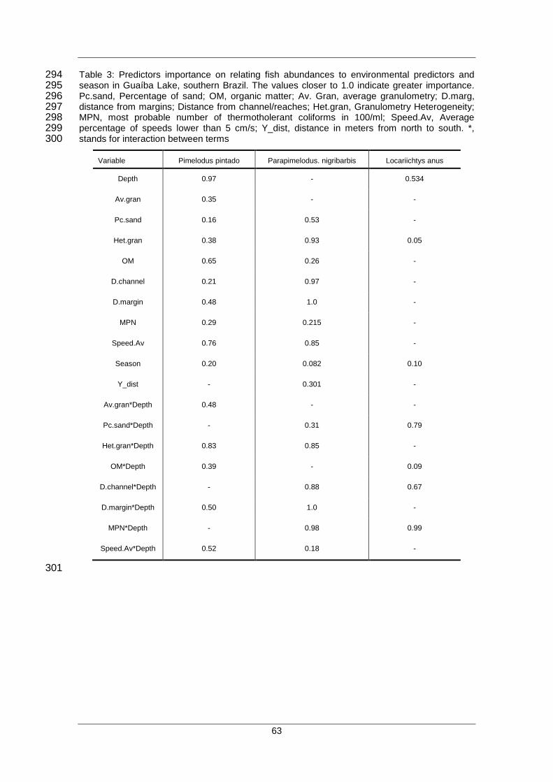
63
Table 3: Predictors importance on relating fish abundances to environmental predictors and 294 season in Guaíba Lake, southern Brazil. The values closer to 1.0 indicate greater importance. 295 Pc.sand, Percentage of sand; OM, organic matter; Av. Gran, average granulometry; D.marg, 296 distance from margins; Distance from channel/reaches; Het.gran, Granulometry Heterogeneity; 297 MPN, most probable number of thermotholerant coliforms in 100/ml; Speed.Av, Average 298 percentage of speeds lower than 5 cm/s; Y_dist, distance in meters from north to south. *, 299 stands for interaction between terms 300
Variable Pimelodus pintado Parapimelodus. nigribarbis Locariichtys anus
Depth 0.97 - 0.534
Av.gran 0.35 - -
Pc.sand 0.16 0.53 -
Het.gran 0.38 0.93 0.05
OM 0.65 0.26 -
D.channel 0.21 0.97 -
D.margin 0.48 1.0 -
MPN 0.29 0.215 -
Speed.Av 0.76 0.85 -
Season 0.20 0.082 0.10
Y_dist - 0.301 -
Av.gran*Depth 0.48 - -
Pc.sand*Depth - 0.31 0.79
Het.gran*Depth 0.83 0.85 -
OM*Depth 0.39 - 0.09
D.channel*Depth - 0.88 0.67
D.margin*Depth 0.50 1.0 -
MPN*Depth - 0.98 0.99
Speed.Av*Depth 0.52 0.18 -
301
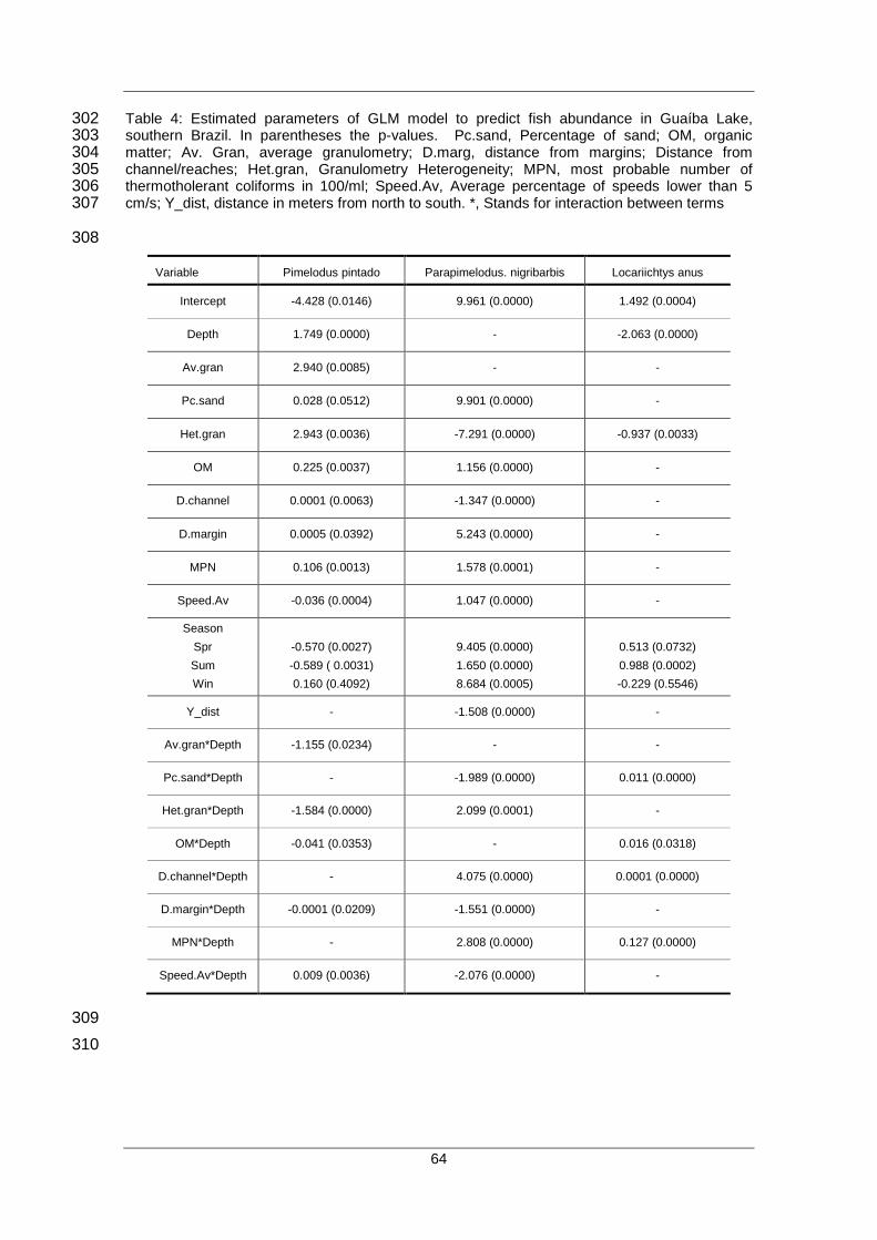
64
Table 4: Estimated parameters of GLM model to predict fish abundance in Guaíba Lake, 302 southern Brazil. In parentheses the p-values. Pc.sand, Percentage of sand; OM, organic 303 matter; Av. Gran, average granulometry; D.marg, distance from margins; Distance from 304 channel/reaches; Het.gran, Granulometry Heterogeneity; MPN, most probable number of 305 thermotholerant coliforms in 100/ml; Speed.Av, Average percentage of speeds lower than 5 306 cm/s; Y_dist, distance in meters from north to south. *, Stands for interaction between terms 307
308
Variable Pimelodus pintado Parapimelodus. nigribarbis Locariichtys anus
Intercept -4.428 (0.0146) 9.961 (0.0000) 1.492 (0.0004)
Depth 1.749 (0.0000) - -2.063 (0.0000)
Av.gran 2.940 (0.0085) - -
Pc.sand 0.028 (0.0512) 9.901 (0.0000) -
Het.gran 2.943 (0.0036) -7.291 (0.0000) -0.937 (0.0033)
OM 0.225 (0.0037) 1.156 (0.0000) -
D.channel 0.0001 (0.0063) -1.347 (0.0000) -
D.margin 0.0005 (0.0392) 5.243 (0.0000) -
MPN 0.106 (0.0013) 1.578 (0.0001) -
Speed.Av -0.036 (0.0004) 1.047 (0.0000) -
Season
Spr
Sum
Win
-0.570 (0.0027)
-0.589 ( 0.0031)
0.160 (0.4092)
9.405 (0.0000)
1.650 (0.0000)
8.684 (0.0005)
0.513 (0.0732)
0.988 (0.0002)
-0.229 (0.5546)
Y_dist - -1.508 (0.0000) -
Av.gran*Depth -1.155 (0.0234) - -
Pc.sand*Depth - -1.989 (0.0000) 0.011 (0.0000)
Het.gran*Depth -1.584 (0.0000) 2.099 (0.0001) -
OM*Depth -0.041 (0.0353) - 0.016 (0.0318)
D.channel*Depth - 4.075 (0.0000) 0.0001 (0.0000)
D.margin*Depth -0.0001 (0.0209) -1.551 (0.0000) -
MPN*Depth - 2.808 (0.0000) 0.127 (0.0000)
Speed.Av*Depth 0.009 (0.0036) -2.076 (0.0000) -
309
310

65
311
312
Figure 6: Abundance map of Pimelodus pintado (Log) predicted with the GLM model relating 313 environmental predictors and season. The scatter plot shows the observed values in relation to 314 the fitted values of GLM model and the values of the predicted abundance map. 315

66
316
Figure 7: Abundance map of Parapimelodus nigribarbis (Log) predicted with the GLM model 317 relating environmental predictors and season. The scatter plot shows the observed values in 318 relation to the fitted values of GLM model and the values of the predicted abundance map. 319

67
320
Figure 8: Abundance map of Loricariichthys anus (Log) with the GLM model relating 321 environmental predictors and season. The scatter plot shows the observed values in relation to 322 the fitted values of GLM model and the values of the predicted abundance map. 323
324

68
Discussion 325
The observed abundance of P. pintado at each sampling point (Fig. 2) and the 326
predicted one (Fig. 6) show a pattern of low abundance close to the margins and 327
higher abundance in deeper areas. The most important predictors were Depth diversity 328
of grain sizes interacting with Depth, Average percentage of speeds lower than 5 cm/s 329
and Organic Matter. According to the coefficients adjusted to P. pintado increased 330
abundance in deeper areas, with sediment characteristics mixing sand granulometry 331
(increased diversity of grains sizes) with some degree of organic matter content. 332
According to DEI TOS et al., (2002) in the Corumbá Reservoir, for Pimelodus 333
maculatus where the species were caught mainly in lotic habitats like small rivers with 334
considerably water flow. In Lake Guaíba the highest water speed is found near to the 335
navigation channel (LERSCH et al., 2013), which is the central part of the lake, 336
justifying the observed distributional pattern in this habitat characteristic influencing the 337
preference of P. pintado. The prediction of P. pintado abundances showed a tendency 338
to occur in deeper areas with more OM. We also observed higher predicted abundance 339
in the upper part of the Lake, where exists significant dumping of nutrients from 340
domestic sewage (Lersch et al., 2013), suggesting a search for food resources. 341
Although the predictor thermotholerant bacteria was not important in the final model. 342
The observed P. nigribarbis abundance (Fig. 7) shows clearly a pattern of higher 343
abundance near to margins and tributaries, with also increased. The map derived from 344
the fitted model shows this pattern, higher abundances in the northeast sector, from the 345
near margins to around the navigation channel and fewer abundance in the middle part 346
of the lake, except where the MPN have moderate to elevated values near to the 347
central part of the lake. The predictors that had the strongest influence in the model 348
were D.margin (importance=1.0; coefficient=5.243), D.channel (importance=0.97; 349
coefficient=-1.347), Speed.Av (importance=0.85; coefficient=1.047), and MPN*Depth 350
(importance =0.98; coefficient=1.749). Besides a pattern of increased abundance near 351
the cetral part of the lake, P. nigribarbis was caught near margins, and associated with 352
low water speeds, in this study, our model results and spatial predictions are in 353
agreement with Dufech and Fialho (2009), Marques et al. (2007) and Lucena et al. 354
(1992). The similar results concern the most important predictors in this work: 355
D.channel, D.margin and MPN*Depth. It was observed that the higher predicted 356
abundance occurs mostly in the northeastern central part of the Lake, in areas 357
corresponding to moderate to higher values of MPN and higher values of Organic 358
Matter (see supplementary material). This pattern suggests the positive influence of 359
69
MPN*depth described by the model (Tab. 4), once this area is could be a source of 360
food. According to Lucena et al. (1992) a planktivorous habit was observed in this 361
species, which could reinforce the reason of high abundances in the region 362
comprehending elevated MNP values. The relationship of P. nigribarbis to MPN 363
suggests a possible use of this species for water monitoring in Guaíba Lake. 364
The best performance to predict the abundance L. anus was achieved through 365
GLM method. Observing the abundance pattern of L. anus (Fig. 2), increased values 366
are observed in the central channel) was found the predominance of occurrences in the 367
in limnetic zones and some selected locations close to the main urban areas. The most 368
important predictors were MPN*depth, PC.sand*depth and D.channel*Depth.. The 369
MPN*depth achieves the highest values in in the northeastern segment of the Guaíba 370
Lake, just by the sides of a large urban area (Porto Alegre city), indicating positive 371
influence of some level of organic pollution associated with deeper waters. Other 372
punctual marginal areas with increased abundances could be related to urban 373
occupation (as Guaíba city), or small river mouths carrying some organic pollution. In 374
the other hand, the species presented also high abundances in the southwestern 375
border of Guaíba Lake, an unpolluted area but with increased organic matter in 376
sediments (supplementary material), although OM had no significance in the adjusted 377
model suggests a preference concerning omnivorous and zoobenthiphagous species 378
(Grosman et al., 1996; Petry and Schulz, 2000). 379
In this work both method selection and model selection were carried out to predict 380
fish abundance in Guaíba Lake. The GAM method was the second best to predict 381
abundances for the three fish species. The GAM selection approach consisted in a 382
forward selection keeping the best models based on the UBRE value. The obtained 383
results were models with few predictors to all species, however the performance was 384
not the best when compared with GLM, except for L. anus, with similar performance for 385
all the tested methods. 386
Although GAM method has the capacity of fitting models to non-linear relationships 387
between predictors and response variable, (Franklin e Miller, 2009; Wood, 2006), there 388
is no automatic model selection procedures like in GLM, for example. The drawback to 389
using GAM with several predictors and few observations is that it requires experience 390
from the modeler to set the number of knots for smoothing procedures. Besides that, 391
the technique had been used and compared with different methods in spatial 392
distribution studies with satisfactory results to model distributions (Segurado and 393
Araújo, 2004; Borchers et al., 1997; Schismenou et al., 2008). On the other hand, GLM 394

70
and BRT have both functions to automate the model selection and evaluation, which 395
facilitates the application in SDM analysis. Considering the characteristics of our data 396
set we considered that the GAM method could be more suitable if the modeler have 397
few predictors and more observations. 398
The GLM method had the best performance to model the abundance for the three 399
species. In this work it was used backward elimination in order to select the best GLM 400
model based in AIC values. Some of predictors in the model had interactions with 401
depth, what caused an increased number of predictors such as Av.gran*depth, 402
Pc.sand*depth, OM*depth, Het.gran*depth, MPN*depth, D.margin*depth, and 403
D.channel*depth. Despite the final models for P. pintado and P. nigribarbis had several 404
predictors they achieved higher r squared, obtaining a better fit and more accuracy. 405
Among the three techniques, the BRT method had unsatisfactory results to model the 406
abundances of at least two fish, P. pintado and P. nigribarbis. GAM and BRT were 407
efficient to model L. anus abundance, however not as well as GLM probably because 408
the lack of predictors interaction. 409
In order to present a set of maps predicting the spatial distribution of fish in Guaíba 410
Lake, predictors obtained from point samples were interpolated for the whole lake area, 411
which bring some bias derived from interpolation technics. Due these biases, the 412
environmental layers do not correspond exactly to the same values at each sampling 413
point. The Figures 6 to 8 show scatter plots of the fitted values originated from the 414
model and the values extracted from the maps. As can be observed, predicted 415
abundances are far more accurate than mapped ones. Nevertheless, the general 416
pattern of the fish distribution, as presented in maps should be interpreted as a 417
collinear result with habitat suitability and the loose of abundance prediction does not 418
compromise the quality of results as an indication of general patterns. 419
Spatial distribution modeling used to predict species distributions and abundance is 420
a powerful method to understand fish relation with several environmental descriptors. 421
Concerning the modeling techniques, it is worth to evaluate more than one 422
methodology, because a single response derived from a single model could hide a 423
response that a particular method can detect. Several studies use this approach to 424
compare at least two methods, exploring the capabilities of each one (Moisen and 425
Frescino, 2002; Thuiller, 2003; Lawler et al., 2006; Leathwick et al., 2006). In this work 426
we presented a comparison among a method able to fit models to non-linear response, 427
a machine learning approach and a classic linear methodology. The models presented 428

71
different outcomes, being dissimilar for P. pintado, and more similar for P. nigribarbis 429
and L. anus. 430
The prediction of P. pintado abundances showed a tendency to occur in deeper 431
areas with more OM. We also observed higher predicted abundance in the upper part 432
of the Lake, where exists significant dumping of nutrients from domestic sewage 433
(Lersch et al., 2013), suggesting a search for food resources. The predictions of P. 434
nigribarbis showed a pattern to occur close to the margins, as well as in regions 435
associated with water pollution from the main urban areas. This pattern suggests that 436
this species could be an indicator of water quality, once the MPN importance in the 437
model was high. The abundance of L. anus was associated to MPN*Depth and 438
Pc.sand*Depth, considering that this species is omnivorous associated to benthic 439
habitats, so the relation to this kind of habitat that attract several macroinvertebrates 440
makes sense.(REF?) 441
Our results, derived from predictors associated with sediment and distances from 442
spatial structures, were relatively easy to create and manipulate to forecast future 443
scenarios in Guaíba Lake. Environmental layers produced by the Lersch et al., (2013) 444
significantly contributed to the applicability of the models concerning future alterations 445
in water quality, and how they could imply in changing fish distributional patterns. In 446
this regard, our results are a stepping-stone in the study of habitat suitability for fish in 447
the Guaíba Lake, once it could forecast future scenarios by modifying the 448
environmental layers for prediction, being a powerful tool for environmental managers. 449
450
Acknowledgements 451
The authors would like to thank the Conselho Nacional de Desenvolvimento 452
Científico e Tecnológico (CNPq) as well as, all the students from Aquatic Ecology Lab 453
who helped in the fieldwork and in the samples processing. We also thank also Babak 454
Naimi and Florian Zellweger for coding suggestions, Departamento Estadual de Portos 455
Rios e Canais (DEPREC) for kindly providing the historical data of Guaíba Lake level 456
readings and Cesar Hoffmann (DMAE) for the information concerning some predictors 457
used in this work. 458
459

72
References 460
Araújo, M. B., Guisan, A. (2006) Five (or so) challenges for species distribution 461
modelling. J. Biogeogr.. 33, 1677–1688. 462
Artioli, L. G. S., Vieira, J. P., Garcia, M., Bemvenuti, M. A. (2009) Distribuição, 463
dominância e estrutura de tamanhos da assembleia de peixes da lagoa Mangueira, sul 464
do Brasil. Iheringia, Sér Zool. 99, 409–418. 465
Azpelicueta, de las M. M., Lundberg, J. G., Loureiro, M. (2008) Pimelodus pintado 466
(Siluriformes: Pimelodidae), a new species of catfish from affluent rivers of Laguna 467
Merín, Uruguay, South America. Proc. Acad. Nat. Sci. Philadelphia. 157, 149–162. 468
Bemvenuti, M. D. A., Moresco, A. (2005) Peixes: áreas de banhados e lagoas 469
costeiras do extremo sul do Brasil. Editora ABRH, Porto Alegre. 470
Borcard, D., Gillet, F., Legendre, P. (2011) Numerical ecology with R. (ed 1 Ed.). 471
Springer New York, New York. 472
Borchers, D. L., Buckland, S. T., Priede, I. G., Ahmadi, S. (1997) Improving the 473
precision of the daily egg production method using generalized additive models. Can. 474
J. Fish. Aquat. Sci.. 54, 2727–2742. 475
Breiman, L., Friedman, J. H., Olshen, R. A., Stone, C. J. (1984) Classification and 476
Regression Trees. (ed C. Hall Crc). Wadsworth. 477
CECO UFRGS, DMAE (1999) Relatório Final do Projeto Sedimentação do Complexo 478
do Guaíba. Porto Alegre. 479
De’ath, G., Fabricius, K. E. (2000) Classification and regression trees: a powerful yet 480
simple technique for ecological data analysis. Ecology. 81, 3178–3192. 481
Dei Tos, C., Barbieri, G., Agostinho, A. A., Gomes, L. C., Suzuki, H. I. (2002) Ecology 482
of Pimelodus maculatus (Siluriformes) in the Corumbá reservoir, Brazil. Cybium. 26, 483
275–282. 484
Douglas, J., Hunt, T., Abery, N., Allen, M. (2009) Application of GIS modelling to 485
quantify fish habitats in lakes. Lakes Reserv. Res. Manag. 14, 171–174. 486

73
Dufech, A. P. S., Fialho, C. B. (2009) Estudo comparado da taxocenose de peixes em 487
dois ambientes aquáticos do Parque Estadual de Itapuã , sul do Brasil. Iheringia. Série 488
Zool.. 99, 177–188. 489
Elith, J., Leathwick, J. R., Hastie, T. (2008) A working guide to boosted regression 490
trees. J. Anim. Ecol.. 77, 802–13. 491
Flores-Lopes, F., Thomaz, A. T. (2011) Histopathologic alterations observed in fish gills 492
as a tool in environmental monitoring. Braz. J. Biol.. 71, 179–88. 493
Franklin, J., Miller, J. A. (2009) Mapping species distributions: spatial inference and 494
prediction. Cambridge University Press Cambridge, UK, New York. 495
Grosman, M. F., González Castelain, J. R., Usonof, E. J. (1996) Trophic niches in an 496
Argentine pond as a way to assess functional relationships between fishes and other 497
communities. Water SA. 22, 345–350. 498
Guisan, A., Thuiller, W. (2005) Predicting species distribution: offering more than 499
simple habitat models. Ecol. Lett.. 8, 993–1009. 500
Guisan, A., Zimmermann, N. E. (2000) Predictive habitat distribution models in 501
ecology. Ecol. Modell.. 135, 147–186. 502
Hasenack, H., Weber, E. (org.) . (2010) Base Cartográfica vetorial contínua do Rio 503
Grande do Sul - escala 1:50.000. 504
Hastie, T., Tibshirani, R. (2008) The elements of statistical learning: data mining, 505
inference and prediction. 2 ed. Ed. Springer. 506
Hiemstra, P. H., Pebesma, E. J., Twenhöfel, C. J. W., Heuvelink, G. B. M. (2009) Real-507
time automatic interpolation of ambient gamma dose rates from the Dutch radioactivity 508
monitoring network. Comput. Geosci.. 35, 1711–1721. 509
Hijmans, R. J., Etten, J. van (2012) raster: Geographic analysis and modeling with 510
raster data. R package version 2.0-12. 511
Hirzel, A. H., Le Lay, G. (2008) Habitat suitability modelling and niche theory. J. Appl. 512
Ecol.. 45, 1372–1381. 513

74
Hirzel, A. H., Le Lay, G., Helfer, V., Randin, C., Guisan, A. (2006) Evaluating the ability 514 of habitat suitability models to predict species presences. Ecol. Modell.. 199, 142–152. 515
Hirzel, A. H., Guisan, A. (2002) Which is the optimal sampling strategy for habitat 516 suitability modelling. Ecol. Modell.. 157, 331–341. 517
Lawler, J. J., White, D., Neilson, R. P., Blaustein, A. R. (2006) Predicting climate-518
induced range shifts: model differences and model reliability. Glob. Chang. Biol.. 12, 519
1568–1584. 520
Leathwick, J. R., Elith, J., Francis, M. P., Hastie, T., Taylor, P. (2006) Variation in 521
demersal fish species richness in the oceans surrounding New Zealand: an analysis 522
using boosted regression trees. Mar. Ecol. Prog. Ser. doi: 10.3354/meps321267. 523
Lersch, E. C., Hoffmann, C. X., Rosman, P. C. C. (2013) II Relatório complementar de 524
avaliação de impacto do Projeto Socioambiental. Porto Alegre. 525
Liaw, A., Wiener, M. (2002) Classification and Regression by randomForest. R News. 526
2, 18–22. 527
Luz-Agostinho, K. D. G., Bini, L. M., Fugi, R., Agostinho, A. A., Júlio Jr., H. F. (2006) 528
Food spectrum and trophic structure of the ichthyofauna of Corumbá reservoir, Paraná 529
river Basin, Brazil. Neotrop. Ichthyol.. 4, 61–68. 530
Lucena, C. A. S., Malabarba, L. R.; Reis, R. E. (1992) Ressurection of the Neotropical 531
Pimemolidae Catfish Parapimelodus nigribarbis (Boulenger), with a phylogenetic 532
diagnosis of the genus Parapimelodus (Teleostei: siluriformes). 533
Maia, B. P., Ribeiro, S. M. F., Bizzotto, P. M., Vono, V., Godinho, H. P. (2007) 534
Reproductive activity and recruitment of the yellow-mandi Pimelodus maculatus 535
(Teleostei: Pimelodidae) in the Igarapava Reservoir, Grande River, Southeast Brazil. 536
Neotrop. Ichthyol.. 5, 147–152. 537
Marques, C. da S., Braun, A. S., Fontoura, N. F. (2007) Estimativa de tamanho de 538
primeira maturação a partir de dados de IGS: Oligosarcus jenynsii, Oligosarcus 539
robustus, Hoplias malabaricus, Cyphocharax voga, Astyanax fasciatus 540
(Characiformes), Parapimelodus nigribarbis, Pimelodus maculatus, Trachelyopterus 541
lucenai, Biocien.. 15, 230–256. 542

75
Miller, J. R., Turner, M. G., SmithWick, E. A. H., Dent, C. L., Stanley, E. H. (2004) 543
Spatial extrapolation: the science of predicting ecological patterns and processes. 544
Bioscience. 54, 310–320. 545
Moisen, G., Frescino, T. (2002) Comparing five modelling techniques for predicting 546
forest characteristics. Ecol. Modell.. 157, 209–225. 547
Moresco, A., Benvenuti, M. de A. (2005) Morphologic features and feeding analysis of 548
the black catfish Trachelyopterus lucenai (Siluriformes, Auchenipteridae ). Acta Limnol. 549
Bras.. 17, 37–44. 550
Nicolodi, J. L., Toldo Jr, E. E., Farina, L. (2011) Wave dynamics and resuspension in 551
Lake Guaíba (Brazil) with implications on points of water abstraction for human supply. 552
J. Coast. Res., 1550–1554. 553
Pebesma, E. J., Bivand, R., Rowlingson, B., Gomez-Rubio, V. (2014) Package “ sp .” 554
http://CRAN.R-project.org/package=sp 555
Peters, D. P. C., Herrick, J. E. (2004) Strategies for ecological extrapolation. Oikos. 556
106, 627–636. 557
Peterson, A. T., Soberón, J., Pearson, R. G., Anderson, R. P., Martínez-Meyer, E., 558
Nakamura, M., Araújo, M. B. (2011) Ecological niches and geographic distributions. Ed. 559
I. Priceton University Press, New Jersey. 560
Petry, A. C., Schulz, U. H. (2000) Ritmo de alimentação dejuvenis de Loricariichthys 561
anus (Siluriformes, Locariidae) da lagoa do Quadros, RS, Brasil. Iheringia. Série Zool. 562
QGIS Development Team (2014) QGIS Geographic Information System. Open Source 563
Geospatial Foundation Project. http://qgis.osgeo.org. qgisorg. 564
R Core Team (2014) R: A language and environment for statistical computing (Version 565
3.03). Foundation for Statistical Computing, Vienna, Austria. URL http://www.R-566
project.org/. 567
Ridgeway, G. (2013) gbm: Generalized Boosted Regression Models. R package 568
version 2.1. URL http://CRAN.R-project.org/package=gbm 569

76
Ramos, I., Vidotto-Magnoni, A., Brandão, H. (2011) Feeding, reproduction and 570
population structure of Pimelodus maculatus Lacépéde, 1803 (Teleostei, Siluriformes, 571
Pimelodiae) from Paraná basin. Bol. da Soc. Bras. Limnol.. 39, 1–15. 572
RStudio (2012). RStudio: Integrated development environment for R (Version 573
0.96.122). Boston, MA. Retrieved May 20, 2012. URL http://www.rstudio.org/ 574
Schismenou, E., Giannoulaki, M., Valavanis, V. D., Somarakis, S. (2008) Modeling and 575
predicting potential spawning habitat of anchovy (Engraulis encrasicolus) and round 576
sardinella (Sardinella aurita) based on satellite environmental information. 577
Hydrobiologia. 612, 201–214. 578
Segurado, P., Araujo, M. B. (2004) An evaluation of methods for modelling species 579
distributions. J. Biogeogr. (J. Biogeogr.). 31, 1555–1568. 580
Sourcepole (2014) OpenLayers 1.3.1. 581
Sutherland, W. J., Freckleton, R. P., Godfray, J. H. C., Beissinger, S. R., Benton, T., 582
Cameron, D. D., Carmel, Y., Coomes, D. A., Coulson, T., Emmerson, M. C., Hails, R. 583
S., Hays, G. C., Hodgson, D. J., Hutchings, M. J., Johnson, D., Jones, J. P. G., 584
Keeling, M. J., Kokko, H., Kunin, W. E., Lambin, X.. (2013) Identification of 100 585
fundamental ecological questions. J. Ecol. doi: 10.1111/1365-2745.12025. 586
Thuiller, W. (2003) BIOMOD - optimizing predictions of species distributions and 587
projecting potential future shifts under global change. Glob. Chang. Biol.. 9, 1353–588
1362. 589
Thuiller, W., Lafourcade, B., Engler, R., Araújo, M. B. (2009) BIOMOD - a platform for 590
ensemble forecasting of species distributions. Ecography (Cop.).. 32, 369–373. 591
Valavanis, V. D., Georgakarakos, S., Kapantagakis, A., Palialexis, A., Katara, I. (2004) 592
A GIS environmental modelling approach to essential fish habitat designation. Ecol. 593
Modell.. 178, 417–427. 594
Villela, I. V., de Oliveira, I. M., Silveira, J. C., Dias, J. F., Henriques, J. A. P., da Silva, 595
J. (2007) Assessment of environmental stress by the micronucleus and comet assays 596
on Limnoperna fortunei exposed to Guaíba hydrographic region samples (Brazil) under 597
laboratory conditions. Mutat. Res.. 628, 76–86. 598
77
Wood, S. N. (2001) mgcv: GAMs and Generalized Ridge Regression for R. R news. 599
Wood, S. N. (2006) Generalized Additive Models: an introduction with R. 600
Zuur, A. F., Leno, E. N., Walker, N. J., Saveliev, A. A., Smith, G. M. (2009) Mixed 601
Effects Models and Extensions in Ecology with R. 1st edn. Springer New York, New 602
York. 603
______________________________________________________
SUPPLEMENTARY MATERIAL
Supplementary material 1 – maps of predictors used in the work (p. 94)
______________________________________________________
78
CONCLUSÕES
Contribuição para a pesquisa no Lago Guaíba
Os primeiros estudos sobre a ictiofauna do lago Guaíba deram início com as
coletas realizados Herbert Huntingdon Smith, em 1881, e John D. Haseman em 1919
(MALABARBA, 1989). Estas foram as primeiras campanhas de amostragem no lago
Guaíba de onde foram descritas diversas espécies para a região. Entre 1919 e 1980 a
produção científica para a região do Guaíba foi muito incipiente, limitando-se aos
resultados das coletas realizadas entre 1881 e 1919 (MALABARBA, 1989). A partir de
1981 dois grupos de pesquisa se consolidam para o estudo da ictiofauna do Rio
Grande do Sul, a Universidade Federal do Rio Grande do Sul (UFRGS) e o Museu de
Ciências e Tecnologia da PUCRS, publicando a maioria dos trabalhos realizados para
o Lago Guaíba e Laguna do Patos (MALABARBA, 1989). Diversas publicações de
cunho sistemático foram produzidas e atualmente a ictiofauna da região está bem
documentada (REIS et al., 2003). Considerando a base sistemática produzida para a
região, trabalhos aplicando o conhecimento já disponível começam a ser publicados.
Estudos foram desenvolvidos visando o uso da ictiofauna como bioindicador da
qualidade da água na região do lago Guaíba (FLORES-LOPES e CETRA, 2010;
FLORES-LOPES e THOMAZ, 2011; FLORES-LOPES, 2011; FLORES-LOPES et al.,
2001). O trabalho realizado por Marques et al. (2007) abordou o tamanho de primeira
maturação das principais espécies de peixe da região, e Treco et al. (2008) realizou
estudos de citogenética em P. nigribarbis e P. pintado lago Guaíba.
Os invertebrados aquáticos, ou macroinvertebrados bentônicos, também foram
alvo de estudos. No trabalho realizado por Focht e Veitenheimer-Mendes (2001) foi
descrita a distribuição sazonal e dinâmica populacional de Neocorbicula limosa.
Mansur e Pereira (2006) estudaram os bivalves ocorrente na bacia do Rio dos Sinos e
Kapusta & Freitas (2012) apresentam a relação entre Limnoperna fortunei e outros
invertebrados no Rio Jacuí. O trabalho realizado por Gonçalves e Skuff (2011) sucita
uma possível relação de C. fluminea e N. limosa com preditores ambientais,
considerando a qualidade da água do lago e fisionomia de fundo.
Considerando os estudos presentes com relação à fauna aquática, invertebrados
bentônicos e peixes, este trabalho foi o primeiro a relacionar a distribuição espacial
dos organismo estudados com preditores ambientais para fins de modelagem de
distribuição. Os resultados gerados com o desenvolvimento deste trabalho iniciam
79
uma nova linha de trabalho na região do Lago Guaíba: a modelagem estatística da
distribuição de espécies. Desta maneira, esse passo somente foi possível a partir do
conhecimento prévio gerado desde as primeiras coletas datadas desde 1881 até os
trabalhos das dezenas de pesquisadores a cerca da fauna aquática da região. Sendo
assim, a comunidade científica e órgãos de fiscalização ambiental podem se beneficiar
no futuro com os dados aqui produzidos com vistas à conservação dos ecossistemas
aquáticos locais.
Impactos ambientais no Lago Guaíba e aplicabilidade dos modelos de
distribuição espacial
A vantagem de se desenvolver a modelagem ecológica, neste caso modelos de
distribuição espacial aplicados a organismos aquáticos, reside no fato que os
resultados obtidos podem ser usados para previsão de cenários futuros, bem como
entender o comportamento das espécies modeladas. No lago Guaíba e região
adjacente, é conhecida a relação negativa da qualidade da água em função da
proximidade de centros urbanos, como a cidade de Porto Alegre, resultando em um
aumento da poluição orgânica (Anexo 1, p.100) - mapa de Coliformes Termo
Tolerantes). A porção norte do Lago, junto ao Delta do Jacuí, apresenta a pior
qualidade de água, segundo os dados Bendati et al. (2000) e a modelagem
apresentada por Lersch et al. (2013). Os dados apresentados quanto a distribuição
espacial dos organismos revelam que a poluição orgânica teve um forte influência nos
modelos apresentados para P. pintado e P. nigribarbis, mesmo que positivamente.
Visto que essa variável pode ser modificada para diferentes cenários ambientais, os
resultados aqui apresentados podem ser usados para estimar as alterações na
distribuição destas espécies.
Outra aplicação dos resultados apresentados aqui repercurtem no âmbito da
alteração da superficie de fundo. No Lago Guaíba ainda não se tem informações a
respeito da mineração de areia para fins de contrução civil. Atualmente, somente o
canal central é dragado para fins de navegação. Levando-se em consideração a
alteração de fundo como um possível impacto, a modelagem preditiva pode ser
empregada como ferramenta para tomada de decisão por órgãos ambientais. Essa
aplicação reforça a necessidade da modelagem em estudos ambientais para a
predição de possíveis impactos. Os trabalhos realizado por Alves e Fontoura (2009),
Barradas et al. (2012) e Rodrigues et al. (2012) enfatizam essa aplicação voltada a
tomada de decisão por ógãos ambientais.

80
Metodologia empregada para o desenvolvimento de mod elos de distribuição
espacial
Atualmente estão disponíveis, em softwares aplicados à estatística, diversas
metodologias que podem ser aplicadas aos modelos de distribuição espacial. Um
ponto positivo a cerca dos diferentes métodos de modelagem é que maioria destes
pode ser usada em softwares livres, tais como o R (R CORE TEAM, 2014). Levando
em consideração a atual disponibilidade dos mais diferentes pacotes estatísticos, fica
a cargo do usuário escolher a metodologia mais adequada ao tipo de dado que se tem
a disposição. Neste estudo, usamos três metodologias: Generalized Addititive Models
(GAM), Generalized Linear Models (GLM) e Boosted Regression Trees (BRT). A
escolha foi realizada com base na natureza dos dados obtidos, e estas metodologias
se mostraram satisfatórias para a modelagem da distribuição das espécies
apresentadas neste estudo.
A metodologia de GAM empregada nos artigos apresentados teve um razoável
rendimento para modelar a distribuição das espécies. A vantagem da metodologia
GAM é a capacidade desta conseguir ajustar modelos com respostas não lineares e
ainda ter uma estatística para avaliação do modelo (GVC e UBRE/AIC). Outra
vantagem deste método é que possível descrever a resposta da variável, sem a
necessidade de muitos preditores. No entanto, a dificuldade encontrada durante a
seleção do melhor modelo relacionou-se à falta de um algoritmo automático para a
seleção de modelo. Com o uso de um número pequeno de preditores, modelagem
GAM se torna viável tendo em vista a menor quantidade de combinações. No entanto,
quando se trata de um número elevado de preditores, o método utilizado por Zuur et
al. (2009) não é dinâmico. Além disto, quando as observações são reduzidas, menores
que 60, e com muitas variáveis adicionais relacionadas à suavização de tendências
não lineares, o código das funções do pacote “mgcv” (WOOD, 2001) tendem a não
convergir adequadamente. O trabalho de Borchers et al. (1997) apresenta o
desenvolvimento da metodologia GAM com número reduzido de preditores, seis
variáveis, e os autores também citaram a dificuldade na seleção do modelo
considerando o tipo de smoother e seleção das variáveis a entrar no modelo final.
Dentre as metodologias disponíveis para os usuários no âmbito do software R,
GLM e BRT são opções robustas e práticas para o uso em modelos de distribuição
espacial. O método GLM possui a disposição uma série de pacotes para ajuste de
modelos, seleção de modelos e visualização. Por se tratar de uma metodologia há
muito tempo testada e sendo normalmente o ponto de partida para análises

81
exploratórias, o método GLM é muito utilizado. A disponibilidade de pacotes estatístico
para seleção de modelos, assim como função step (Backward, Forward), permitem ao
usuário maior rapidez na seleção de modelos, tornando-se um ponto positivo para
aplicação desta metodologia. Além, por se tratar de metodologia de regressão, com
coeficientes numéricos diretamente interpretáveis, esta metodologia apresenta-se
mais transparente ao usuário, permitindo simulação para outros cenários e condições,
através da aplicação direta do modelo em qualquer software estatístico.
Os pacotes estatísticos atualmente disponíveis para o uso do método BRT são
muito robustos em termos de avaliação dos modelos e seleção. A seleção dos
modelos é realizada por validação cruzada além de funções para simplificação dos
modelos (ELITH et al., 2008; HIJMANS; ELITH, 2013). O BRT produz centenas ou
milhares de árvores de decisão, e a solução final não é um consenso, mas a soma das
soluções de cada árvore parcial desenvolvido a partir de um subconjunto de dados.
Sendo assim, configura-se como uma metodologia com alto poder preditivo. De acordo
Elith et al. (2008), a vantagem vem do princípio que a soma de várias regras de
classificação mais flexíveis geralmente superam uma regra com uma única solução
(eg. GLM, GAM), implicando em um fraco desempenho preditivo para outras
localidades.
Predititores Ambientais gerados
Com o intuito de se obter um mapa representando a adequabilidade de hábitat
calculada pelos modelos ajustados para as espécies foco deste trabalho, foram
usadas variáveis que pudessem permitir a construção de mapas ambientais (anexo).
Apesar de ser interessante investigar variáveis que possuem implicação fisiológicas
para algumas espécies, tais como oxigênio dissolvido e condutividade, com estas não
é possível se criar um mapa em função da ampla variabilidade temporal das mesmas.
Portanto, as classes de preditores aqui utilizados compreenderam medidas de
distância, características do sedimento, velocidade de corrente e poluição ambiental.
Estes preditores representam a influência direta e indireta de variáveis que
potencialmente podem influenciar a seleção de hábitat por parte das espécies. A
geração dos mapas de distância (distância da margem e de canais/riachos)
representou a possível influência da complexidade de hábitat (e.g.: rochas, macrófitas
e galhos) que potencialmente podem apresentar uma maior concentração em função
da proximidade com margens e foz de tributários. Essas variáveis foram importantes
no modelo selecionado para P. nigribarbis.

82
Os preditores ambientais caracterizando o sedimento de fundo do Lago Guaíba
foram importantes nos modelos para C. fluminea, P. pintado e P. nigribarbis. Os
preditores caracterizando o perfil granulométrico do sedimento de fundo do Guaíba,
assim como o teor de matéria orgânica foram obtidos pela união da matriz de dados
gerada neste trabalho e os dados gerados pelo projeto de sedimentação do lago
Guaíba (CECO UFRGS; DMAE, 1999). A partir da junção destes dois bancos de
dados foi possível acrescentar mais pontos à matriz de análise, sendo possível
construir mapas ambientais que descreveram a fisionomia de fundo do lago Guaíba.
Além da caracterização convencional de sedimentos, foi proposto o preditor de
diversidade de Shannon dos tamanhos dos grãos de sedimento, baseando-se no
princípio de que a complexidade de hábitat pode influenciar a riqueza de espécies de
macroinvertebrados bentônicos (GILINSKY, 1984; HECK JR e WETSTONE, 1977) e
consequentemente podendo caracterizar-se como uma variável relacionada à seleção
e hábitat para peixes a procura de alimento. Essa variável foi importante para C.
fluminea e P. nigribarbis.
As variáveis considerando aspectos da hidrodinâmica e despejos de esgoto
orgânico foram importantes para a distribuição de alguns organismos apresentados. A
variável velocidade média, consistiu na média da porcentagem das velocidades
menores que 5cm/s das estação seca e chuvosa. Os valores de coliformes
termotolerantes consistem em uma média geral para o lago com base nos dados
fornecidos pelo órgão de saneamento básico do município de Porto Alegre. Os mapas
destas variáveis são advindos do trabalho de Lershc et al. (2013) usando a técnica de
modelagem SisBahia (ROSMAN, 2014). Estas variáveis foram importantes nos
modelos, principalmente para as espécies de peixes P. nigribarbis e L. anus.
A interpolação das variáveis selecionadas e o uso das variáveis disponíveis
possibilitou a realização dos mapas preditivos em pequena escala. Modelagem de
distribuição de espécies comumente é realizada com preditores ambientais obtidos de
imagens de sensoriamento remoto, modelos climáticos (BIOCLIM), modelos de
elevação digital, dentre outras fontes de imagens (FRANKLIN e MILLER, 2009). No
entanto, os métodos convencionais não são capazes de criar preditores em escala
reduzida em ambientes aquáticos, menores que 100 metros de resolução. Esta
limitação na aquisição de dados em escala reduzida em ambientes aquáticos, como
no lago Guaíba, tornou desafiadora a tarefa de se desenvolver a modelagem espacial
com ênfase na adequabilidade de hábitat para as espécies foco deste estudo. Foi
necessária a busca por dados já existentes e a criação das superfícies interpoladas

83
para a geração dos mapas de distribuição espacial. Contornando esse desafio, foi
possível transpor a barreira da inexistência de variáveis detalhadas na escala do lago
e empregar uma metodologia capaz de produzir mapas de adequabilidade de hábitat.
Perspectivas
A partir do trabalho realizado deu-se início a modelagem de distribuição de
espécies no Lago Guaíba, um dos corpos de água mais importantes do sul do Brasil.
Durante nossas campanhas amostramos inúmeras outras espécies que não foram
modeladas para a tese pelo tempo limitado que um curso de doutorado impõe. Desta
maneira, pretende-se aperfeiçoar o processo de análise, assim como modelar as
outras espécies que constam no nosso banco de dados, assim como a diversidade de
espécies.
O Lago Guaíba possivelmente sofrerá mudanças limnológicas sensíveis em futuro
próximo, umas vez que ao longo do desenvolvimento deste trabalho o tratamento de
efluentes lançados no lago aumentou de 26% para 76% com a entrada em operação
da Estação de Tratamento de Efluentes da Serraria. Consequentemente, espera-se
mudanças na qualidade da água e possivelmente a fauna aquática pode ter uma
respostas frente a essa melhoria. Portanto uma das perspectivas deste trabalho é
investigar como a fauna aquática pode responder a essas alterações no âmbito da
modelagem da distribuição de espécies.

84
REFERÊNCIAS
ALVES, T. P.; FONTOURA, N. F. Statistical distribution models for migratory fish in Jacuí basin, South Brazil. Neotropical Ichthyology , v. 7, n. 4, p. 647–658. 2009.\
ARAÚJO, M. Climate change and spatial conservation planning. In: A. Moilanen; K. A. Wilson; H. Possingham (Eds.); Spatial conservation prioritization: Quantitative Methods and Computational Tools . p.328. London: Oxford University Press, 2009.
ARAÚJO, M. B.; FERRI-YÁÑEZ, F.; BOZINOVIC, F.; et al. Heat freezes niche evolution. Ecology letters , v. 16, n. 9, p. 1206–19, 2013.
ARAÚJO, M. B.; NEW, M. Ensemble forecasting of species distributions. Trends in ecology and evolution , v. 22, n. 1, p. 42–47, 2007.
ARTIOLI, L. G. S.; VIEIRA, J. P.; GARCIA, M.; BEMVENUTI, M. A. Distribuição, dominância e estrutura de tamanhos da assembleia de peixes da lagoa Mangueira, sul do Brasil. Iheringia, Sér Zool , v. 99, n. 4, p. 409–418, 2009.
AUSTIN, M. Searching for a model for use in vegetation analysis. Vegetatio , v. 42, n. 1, p. 11–21, 1980.
AUSTIN, M. P. Spatial prediction of species distribution: an interface between ecological theory and statistical modelling. Ecological Modelling , v. 157, n. 2-3, p. 101–118, 2002.
AUSTIN, M.; SMITH, T. A new model for the continuum concept. Vegetatio , v. 83, p. 35–47, 1989.
AZPELICUETA, DE LAS M. M.; LUNDBERG, J. G.; LOUREIRO, M. Pimelodus pintado (Siluriformes: Pimelodidae), a new species of catfish from affluent rivers of Laguna Merín, Uruguay, South America. Proceedings of the Academy of Natural Sciences of Philadelphia. v. 157, p. 149–162, 2008., 2008.
BARBOSA, F. G.; MELO, A. S. Modelo preditivo de sobrevivência do Mexilhão Dourado (Limnoperna fortunei) em relação a variações de salinidade na Laguna dos Patos, RS, Brasil. Biota Neotropica , v. 9, n. 3, p. 407–412, 2009.
BARRADAS, J. R. S.; SILVA, L. G.; HARVEY, B. C.; FONTOURA, N. F. Estimating migratory fish distribution from altitude and basin area: a case study in a large Neotropical river. Freshwater Biology , v. 57, n. 11, p. 2297–2305. 2012.
BENDATI, M. M.; AL, E. Avaliação da qualidade da água do lago Guaíba (Rio Grande do Sul, Brasil) como suporte para a gestão da bacia hidrográfica. XXVII Congresso Interamericano de Engenharia Sanitária e Ambiental. Anais... . p.V–076. Porto Alegre, 2000.
BEWICK, V.; CHEEK, L.; BALL, J. Statistics review 14: Logistic regression. Critical care (London, England) , v. 9, n. 1, p. 112–8, 2005.
BILLICK, I.; CASE, T. Higher Order Interactions in Ecological Communities : What Are They and How Can They be Detected ? Ecology , v. 75, n. 6, p. 1529–1543, 1994.

85
BOOTH, T. H. A climatic analysis method for expert systems assisting tree species introductions. Agroforestry Systems , v. 10, p. 33–45, 1990.
BORCHERS, D. L.; BUCKLAND, S. T.; PRIEDE, I. G.; AHMADI, S. Improving the precision of the daily egg production method using generalized additive models. Canadian Journal of Fisheries and Aquatic Sciences ., 1997.
BREIMAN, L.; FRIEDMAN, J. H.; OLSHEN, R. A.; STONE, C. J. Classification and Regression Trees (C. Hall Crc, Ed.)The Wadsworth statisticsprobability series , Statistics/Probability Series. v. 19, p.368. Wadsworth, 1984.
BREIMAN, L. Statistical Modeling: The Two Cultures. Statistical Science , v. 16, n. 3, p. 199–231, 2001.
BUSBY, J. R. A biogeoclimatic analysis of Nothofagus cunninghamii ( Hook .) Oerst . in southeastern Australia. Australian Journal of Ecology , v. 11, p. 1–7, 1986.
CARPENTER, G.; GILLISON, A.; WINTER, J. DOMAIN : a flexible modelling procedure for mapping potential distributions of plants and animals. Biodiversity and Conservatio , v. 2, p. 667–680, 1993.
CECO UFRGS; DMAE. Relatorio Final do Projeto Sedimentação do Complexo do Guaíba . p.35. Porto Alegre, 1999.
CHEUNG, W. W. L.; SARMIENTO, J. L.; DUNNE, J.; et al. Shrinking of fishes exacerbates impacts of global ocean changes on marine ecosystems. Nature Climate Change , v. 3, n. September 2012, p. 254–258, 2012.
COHEN, R. R. H.; DRESLER, P. V.; PHILLIPS, E. J. P.; CORY, R. L. The effect of the Asiatic clam, Corbicula fluminea, on phytoplankton of the Potomac River, Maryland. Limnology and Oceanography , v. 29, n. 1, p. 170–180, 1984.
CONNELL, J. Diversity in Tropical Raisn Forests and Coral Reefs. Science , v. 199, n. 4335, p. 1302–1310, 1978.
CRAWLEY, M. J. Statistics: An Introduction using RAmerican Statist ician . v. 61, p.327. Chichester: Wiley, 2005.
DE’ATH, G. Boosted trees for ecological modeling and prediction. Ecology , v. 88, n. 1, p. 243–51, 2007.
DE’ATH, G.; FABRICIUS, K. E. Classification and regression trees: a powerful yet simple technique for ecological data analysis. Ecology , v. 81, n. 11, p. 3178–3192, 2000.
DEI TOS, C.; BARBIERI, G.; AGOSTINHO, A. A.; GOMES, L. C.; SUZUKI, H. I. Ecology of Pimelodus maculatus (Siluriformes) in the Corumbá reservoir, Brazil. Cybium , v. 26, n. 4, p. 275–282, 2002.
DOUGLAS, J.; HUNT, T.; ABERY, N.; ALLEN, M. Application of GIS modelling to quantify fish habitats in lakes. Lakes and Reservoirs: Research and Management , v. 14, n. 2, p. 171–174, 2009.

86
DUDÍK, M.; PHILLIPS, S. J.; SCHAPIRE, R. E. Maximum Entropy Density Estimation with Generalized Regularization and an Application to Species Distribution Modeling. Journal of Machine Learning Research , v. 8, p. 1217–1260, 2007.
DUFECH, A. P. S.; FIALHO, C. B. Estudo comparado da taxocenose de peixes em dois ambientes aquáticos do Parque Estadual de Itapuã , sul do Brasil. Iheringia. Série Zoologia , v. 99, n. 1988, p. 177–188, 2009.
ELITH, J.; LEATHWICK, J. R.; HASTIE, T. Boosted Regression Trees in R Overview. , 2008.
ELITH, J.; LEATHWICK, J. Boosted Regression Trees for ecological modeling. , 2012.
ELITH, J.; LEATHWICK, J. R.; HASTIE, T. A working guide to boosted regression trees. The Journal of animal ecology , v. 77, n. 4, p. 802–13, 2008.
ELITH, J.; PHILLIPS, S. J.; HASTIE, T.; et al. A statistical explanation of MaxEnt for ecologists. Diversity and Distributions , v. 17, p. 43–57. doi, 2011.
FRANKLIN, J.; MILLER, J. A. Mapping species distributions: spatial inference an d predictionJournal of Tropical Ecology . p.340. New York: Cambridge University Press Cambridge, UK, 2009.
ELTON, C. Animal EcologyAnimal ecology . v. New impres, p.207. London: Sidgwick and Jackson. doi: 10.1098/rstb.2010.0107, 1927.
FLORES-LOPES, F. Frequency of morphological alterations in the fish of Lake Guaíba and its application to environmental monitoring. Bioikos , v. 25, n. 1, p. 11–23, 2011.
FLORES-LOPES, F.; CETRA, M. Utilização de índices ecológicos em assembléias de peixes como instrumento de avaliação da degradação ambiental em programas de monitoramento. Biota Neotropica , v. 10, n. 4, p. 183–193, 2010.
FLORES-LOPES, F.; MALABARBA, L. R.; PEREIRA, E. H. L.; SILVA, J. F. P. DA. Alterações histológicas em placas ósseas do peixe cascudo Rineloricaria strigilata (Hensel) (Teleostei, Loricariidae) e sua frequência no lago Guaíba, Rio Grande do Sul, Brasil. Revista Brasileira de Zoologia , v. 18, n. 3, p. 699–709. 2001.
FLORES-LOPES, F.; THOMAZ, A. T. Histopathologic alterations observed in fish gills as a tool in environmental monitoring. Brazilian journal of biology = Revista brasleira de biologia , v. 71, n. 1, p. 179–88, 2011.
FOCHT, T.; VEITENHEIMER-MENDES, I. L. Distribuição sazonal e reprodução de Neocorbicula limosa (Maton) (Bivalvia, Corbiculidae) no Lago Guaíba, Rio GRande do Sul, Brasil. Revista Brasileira de Zoologia , v. 18, n. 1, p. 35–43, 2001.
FORDHAM, D. A.; AKÇAKAYA, H. R.; BROOK, B. W.; et al. Adapted conservation measures are required to save the Iberian lynx in a changing climate. Nature Climate Change , v. 3, n. 10, p. 899–903, 2013.
FRAGOSO JR., C. R.; FERREIRA, T. F.; MARQUES, D. M. L. D. M. Modelagem Ecológica em Ecossistemas Aquáticos . p.304, 2009.

87
FRANKLIN, J. Predictive vegetation mapping: geographic modelling of biospatial patterns in relation to environmental gradients. Progress in Physical Geography , v. 19, n. 4, p. 474–499, 1995.
FRANKLIN, J.; MILLER, J. A. Mapping species distributions: spatial inference an d predictionJournal of Tropical Ecology . p.340. New York: Cambridge University Press Cambridge, UK, 2009.
FRIEDMAN, J. H.; MEULMAN, J. J. Multiple additive regression trees with application in epidemiology. Statistics in medicine , v. 22, n. 9, p. 1365–81. doi: 10.1002/sim.1501, 2003.
GAHEGAN, M. Is inductive machine learning just another wild goose (or might it lay the golden egg)? International Journal of Geographical Information S cience , v. 17, n. 1, p. 69–92, 2003.
GERMAN, G. W. H.; GAHEGAN, M. N. Neural network architectures for the classification of temporal image sequences. Computers & Geosciences , v. 22, n. 9, p. 969–979, 1996.
GILINSKY, E. The Role of Fish Predation and Spatial Heterogeneity in Determining Benthic Community Structure. Ecology , v. 65, n. 2, p. 455–468, 1984.
GONÇALVES, L.; SKUFF, T. Distribuição e Abundância dos Bivalves Corbicula fluminea (Mueller, 1774) e Neocorbicula limosa (Maton, 1811) no Lago Guaíba, Rio Grande do Sul, Brasil. Fepam em Revista , v. 5, n. 1, p. 13–18, 2011.
GRINNELL, J. The Niche-relationships of the California Thrasher. The Auk , v. 34, n. 4, p. 427–433, 1917.
GUIMARÃES, T. DE F. R.; HARTZ, S. M.; BECKER, F. G. Lake connectivity and fish species richness in southern Brazilian coastal lakes. Hydrobiologia , v. 740, n. 1, p. 207–217, 2014.
GUISAN, A.; ZIMMERMANN, N. E. Predictive habitat distribution models in ecology. Ecological Modelling , v. 135, n. 2-3, p. 147–186. doi: 10.1016/S0304-3800(00)00354-9, 2000.
GUISAN, A.; THUILLER, W. Predicting species distribution: offering more than simple habitat models. Ecology Letters , v. 8, n. 9, p. 993–1009, 2005.
HALTUCH, M.; BERKMAN, P. Geographic information system (GIS) analysis of ecosystem invasion: Exotic mussels in Lake Erie. Limnology and Oceanography , v. 45, n. 8, p. 1778–1787, 2000.
HASTIE, T. J.; TIBSHIRANI, R. Generalized additive modelsStatistical Science . v. 1, p.297–318, 1990.
HASTIE, T.; TIBSHIRANI, R. Generalized Additive Models. Statistical Science , v. 1, p. 297–310,1986.
HASTIE, T.; TIBSHIRANI, R.; FRIEDMAN, J. H. The elements of statistical learning: data mining, inference, and predicition.The Mathema tical … . 2nd ed., p.739. New York, NY: Springer, 2008.

88
HECK JR, K.; WETSTONE, G. Habitat complexity and invertebrate richness and abundance in tropical seagrass meadows. Journal of Biogeography , v. 4, n. 2, p. 135–142, 1977.
HIJMANS, R.; ELITH, J. Species distribution modeling with RR CRAN Project , 2013.
HIRZEL, A. H.; LAY, G. LE. Habitat suitability modelling and niche theory. Journal of Applied Ecology , v. 45, n. 5, p. 1372–1381, 2008.
HIRZEL, A. H.; LAY, G. LE; HELFER, V.; RANDIN, C.; GUISAN, A. Evaluating the ability of habitat suitability models to predict species presences. Ecological Modelling , v. 199, n. 2, p. 142–152, 2006.
HUTCHINSON, G. E. Concluding remarks. Cold Spring Harbour Symposia on Quantitative Biology , v. 22, p. 415–427, 1957.
JACKSON, S. T.; OVERPECK, J. T. Responses of plant populations and communities to environmental changes of the late Quaternary. Paleobiology , v. 26, n. sp4, p. 194–220, 2000.
JAMES, F. C.; JOHNSTON, R. F.; WARMER, N. O.; NIEMI, G. J.; BOECKLEN, W. J. The Grinnellian Niche of the Wood Thrush. The American Naturalist , v. 124, n. 1, p. 17–47, 1984.
KAPUSTA, S. C.; FREITAS, S. M. Limnoperna fortunei na bacia hidrográfica do Rio Jacuí: relações com a comunidade de macroinvertebrados bentônicos. Moluscos límnicos invasores no Brasil : biologia, prevenção, controle . p.243–246, 2012.
KEITH, D. A; AKÇAKAYA, H. R.; THUILLER, W.; et al. Predicting extinction risks under climate change: coupling stochastic population models with dynamic bioclimatic habitat models. Biology letters , v. 4, n. 5, p. 560–3, 2008.
KENDALL, M. S.; CHRISTENSEN, J. D.; HILLIS-STARR, Z. Multi-scale data used to analyze the spatial distribution of French grunts, Haemulon flavolineatum, relative to hard and soft bottom in a benthic landscape. Environmental Biology of Fish , v. 66, p. 19–26, 2003.
KHAN, J.; WEI, J. S.; RINGNÉR, M.; et al. Classification and diagnostic prediction of cancers using gene expression profiling and artificial neural networks. Nature medicine , v. 7, n. 6, p. 673–9, 2001.
KOLOZSVARY, M. B.; SWIHART, R. K. Habitat fragmentation and the distribuition of amphibians: patch and landscape correlates in farmland. Can. J. Zool , v. 77, p. 1288–1299, 1999.
LEATHWICK, J. R.; ELITH, J.; CHADDERTON, W. L.; ROWE, D.; HASTIE, T. Dispersal, disturbance and the contrasting biogeographies of New Zealand’s diadromous and non-diadromous fish species. Journal of Biogeography , v. 35, n. 8, p. 1481–1497, 2008.
LEATHWICK, J. R.; ELITH, J.; FRANCIS, M. P.; HASTIE, T.; TAYLOR, P. Variation in demersal fish species richness in the oceans surrounding New Zealand: an analysis using boosted regression trees. Marine Ecology Progress Series , v. 321, p. 267–281, 2006.

89
LEATHWICK, J. R.; ROWE, D.; RICHARDSON, J.; ELITH, J.; HASTIE, T. Using multivariate adaptive regression splines to predict the distributions of New Zealand ’ s freshwater diadromous fish. Freshwater Biology , v. 50, p. 2034–2052, 2005.
LEIBOLD, M. The Niche Concept Revisited: Mechanistic Models and Community Context. Ecology , v. 76, n. 5, p. 1371–1382, 1995.
LEK, S.; DELACOSTE, M.; BARAN, P.; et al. Application of neural networks to modelling nonlinear relationships in ecology. Ecological Modelling , v. 90, n. 1, p. 39–52. Elsevier, 1996.
LERSCH, E. C.; HOFFMANN, C. X.; ROSMAN, P. C. C. II Relatório complementar de avaliação de impacto do Projeto Socioambiental . p.113. Porto Alegre, 2013.
LEVINS, R. The strategy of model building in population biology. American Scientist , v. 54, n. 4, p. 421–431, 1966.
LUCENA, C. A. S.; MALABARBA, L. R.; REIS, R. E. Ressurection of the Neotropical Pimemolidae Catfish Parapimelodus nigribarbis (Boulenger), with a phylogenetic diagnosis of the genus Parapimelodus (Teleostei: siluriformes). , v. 1, p. 138–146, 1992.
LUZ-AGOSTINHO, K. D. G.; BINI, L. M.; FUGI, R.; AGOSTINHO, A. A.; JÚLIO JR., H. F. Food spectrum and trophic structure of the ichthyofauna of Corumbá reservoir, Neotropical Ichthyology, v. 4, n. 1, p. 61–68, mar. 2006
FERRIER, S.; GUISAN, A.; ELITH, J.; et al. Novel methods improve prediction of species’ distributions from occurrence data. Ecography , v. 29, n. January, p. 129–151, 2006.
KINIPLING, G.W. O Guaíba e a lagoa dos Patos . (G.W. Knipling, Ed.) 3 ed. amp. ed., p.176. Porto Alegre, 2002.
MACLEOD, C. D.; MANDLEBERG, L.; SCHWEDER, C.; BANNON, S. M.; PIERCE, G. J. A comparison of approaches for modelling the occurrence of marine animals. Hydrobiologia , v. 612, n. 1, p. 21–32, 2008.
MAIA, B. P.; RIBEIRO, S. M. F.; BIZZOTTO, P. M.; VONO, V.; GODINHO, H. P. Reproductive activity and recruitment of the yellow-mandi Pimelodus maculatus (Teleostei: Pimelodidae) in the Igarapava Reservoir, Grande River, Southeast Brazil. Neotropical Ichthyology , v. 5, n. 2, p. 147–152, 2007.
NICOLODI, J. L.; TOLDO JR, E. E.; FARINA, L. Wave dynamics and resuspension in Lake Guaíba (Brazil) with implications on points of water abstraction for human supply. Journal of Coastal Research , , n. Special issue 64, p. 1550–1554, 2011.
OLDEN, J. D.; JACKSON, D. A. Fish-Habitat Relationships in Lakes: Gaining Predictive and Explanatory Insight by Using Artificial Neural Networks. Transactions of the American Fisheries Society , v. 130, n. 5, p. 878–897. Taylor & Francis, 2001.
OTTAVIANI, D.; LASINIO, G. J.; BOITANI, L. Two statistical methods to validate habitat suitability models using presence-only data. Ecological Modelling , v. 179, n. 4, p. 417–443, 2004.

90
MACKEY, B. G.; LINDENMAYER, D. B. Towards a hierarchical framework for modelling the spatial distribution of animals. Journal of Biogeography , v. 28, n. 9, p. 1147–1166, 2001.
MALABARBA, L. R. Histórico sistemático e lista comentada das espécies de peixes de água doce do sistema da Laguna dos Patos, Rio Grande do Sul, Brasil. Comunicações do Museu de Ciências e Tecnologia da P UCRS, Sér. Zool. , v. 2, n. 8, p. 107–179, 1989.
MANSUR, M. C. D.; PEREIRA, D. Bivalves límnicos da Bacia do Rio dos Sinos, Rio Grande do Sul, Brasil. Revista Brasileira de Zoologia , v. 23, n. 4, p. 1123–1147, 2006.
MANSUR, M. C. D.; SANTOS, C. P. DOS; PEREIRA, D.; et al. Moluscos líminicos invasores no Brasil: Biologia, prevenção, controle. Moluscos límnicos invasores no Brasil : biologia, prevenção, controle . 1st ed., p.411. Porto Alegre: Redes, 2012.
MANSUR, M. C. D.; SANTOS, C. P. DOS; DARRIGRAN, G.; et al. Primeiros dados quali-quantitativos do mexilhão-dourado, Limnoperna fortunei (Dunker), no Delta do Jacuí, no Lago Guaíba e na Laguna dos Patos, Rio Grande do Sul, Brasil e alguns aspectos de sua invasão no novo ambiente. Revista Brasileira de Zoologia , v. 20, n. 1, p. 75–84, 2003.
MARQUES, C. DA S.; BRAUN, A. S.; FONTOURA, N. F. Estimativa de tamanho de primeira maturação a partir de dados de IGS: Oligosarcus jenynsii, Oligosarcus robustus, Hoplias malabaricus, Cyphocharax voga, Astyanax fasciatus (Characiformes), Parapimelodus nigribarbis, Pimelodus maculatus, Trachelyopterus lucenai. BIOCIÊNCIAS , v. 15, n. 2, p. 230–256, 2007.
MASTRORILLO, S.; LEK, S.; DAUBA, F.; BELAUD, A. The use of artificial neural networks to predict the presence of small-bodied fish in a river. Freshwater Biology , v. 38, n. 2, p. 237–246. Wiley Online Library, 1997.
MILLER, J.; FRANKLIN, J. Modeling the distribution of four vegetation alliances using generalized linear models and classification trees with spatial dependence. Ecological Modelling , v. 157, n. 2-3, p. 227–247, 2002.
MILLER, J. R.; TURNER, M. G.; SMITHWICK, E. A. H.; DENT, C. L.; STANLEY, E. H. Spatial extrapolation: the science of predicting ecological patterns and processes. BioScience , v. 54, n. 4, p. 310–320. BioOne, 2004.
MOISEN, G.; FRESCINO, T. Comparing five modelling techniques for predicting forest characteristics. Ecological Modelling , v. 157, n. 2-3, p. 209–225, 2002.
MORESCO, A.; BENVENUTI, M. DE A. Morphologic features and feeding analysis of the black catfish Trachelyopterus lucenai Bertoletti , Pezzi da Silva & Pereira (Siluriformes, Auchenipteridae). Acta Limnologica Brasiliensia , v. 17, n. 1, p. 37–44, 2005.
NICHOLLS, A. How to make biological surveys go further with generalised linear models. Biological Conservation , v. 50, p. 51–75, 1989.
NICOLODI, J. L. O Padrão de ondas no lago Guaíba e sua influência n os processos de sedimentação . Universidade Federal do Rio Grande do Sul. Instituto de Geociências. Programa de Pós-Graduação em Geociências., 2007.

91
OTTAVIANI, D.; LASINIO, G. J.; BOITANI, L. Two statistical methods to validate habitat suitability models using presence-only data. Ecological Modelling , v. 179, n. 4, p. 417–443, 2004.
PEARCE, J.; FERRIER, S. An evaluation of alternative algorithms for fitting species distribution models using logistic regression. Ecological Modelling , v. 128, n. 2-3, p. 127–147, 2000.
PETERS, D. P. C.; HERRICK, J. E. Strategies for ecological extrapolation. Oikos , v. 106, n. 3, p. 627–636, 2004.
PETERSON, A. T.; SOBERÓN, J.; PEARSON, R. G.; et al. Ecological niches and geographic distributionsChoice Reviews Online . Ed. I ed., v. 49, p.314. New Jersey: Priceton University Press, 2011.
PHILLIPS, S. J.; ANDERSON, R. P.; SCHAPIRE, R. E. Maximum entropy modeling of species geographic distributions. Ecological modelling , v. 190, n. 3-4, p. 231–259. Elsevier, 2006.
PORTER, M. S.; ROSENFELD, J.; PARKINSON, E. A. Predictive models of fish species distribution in the Blackwater drainage, British Columbia. North American Journal of Fisheries Management , v. 20, n. 2, p. 349–359. Taylor and Francis, 2000.
PREZANT, R. S.; CHALERMWAT, K. Flotation of the bivalve Corbicula fluminea as a means of dispersal. Science , v. 225, n. 4669, p. 1491. American Association for the Advancement of Science, 1984.
REIS, R. E.; KULLANDER, S. O.; FERRARIS, C. J. Check List of the Freshwater Fish of South and Central America (R. Reis, S. Kullander, and C. J. Ferraris, Eds.)Copeia . v. 2004, p.714–716. Porto Alegre: Edipucrs, 2003.
R CORE TEAM. R: A language and environment for statistical computing. . R Foundation for Statistical Computing, Vienna, Austria. URL http://www.R-project.org/ ISBN 3-900051-07-0, 2014.
RAMOS, I.; VIDOTTO-MAGNONI, A.; BRANDÃO, H. Feeding, reproduction and population structure of Pimelodus maculatus Lacépéde, 1803 (Teleostei, Siluriformes, Pimelodiae) from Paraná basin. Boletin da Sociedade Brasileira de Limnologia , v. 39, n. 2, p. 1–15, 2011.
RODRIGUES, L.; BARRADAS, J.; ALVES, T.; FONTOURA, N. Modelagem estatística de distribuição de peixes migradores como subsídio ao licenciamento de barramentos na bacia Camaquã, RS. Revista de Gestão de Água da América Latina , v. 8, n. 2, p. 31–41, 2012.
ROSMAN, P. C. C. Referência Técnica do Sistema Base de Hidrodinâmica Ambiental- SisBaHiA, COPPE-UFRJ. Paulo Cesar Colonna Rosman, Ed., 2014.
RODRIGUES, L.; BARRADAS, J.; ALVES, T.; FONTOURA, N. Modelagem estatística de distribuição de peixes migradores como subsídio ao licenciamento de barramentos na bacia Camaquã, RS. Revista de Gestão de Água da América Latina , v. 8, n. 2, p. 31–41, 2012.
ROTENBERRY, J.; PRESTON, K.; KNICK, S. GIS-BASED NICHE MODELING FOR MAPPING SPECIES’HABITAT. Ecology , v. 87, n. 6, p. 1458–1464, 2006.

92
SACCOL-PEREIRA, A.; FIALHO, C. B. Seasonal and diel variation in the fish assemblage of a Neotropical delta in southern Brazil. Iheringia. Série Zoologia , v. 100, n. 2, p. 169–178. SciELO Brasil, 2010.
SALOMONI, S.; TORGAN, L. Epilithic diatoms as organic contamination degree indicators in Guaiba Lake, Southern Brazil. Acta Limnologica Brasiliensia , v. 20, n. 4, p. 313–324, 2008.
SCHAPIRE, R. E. The boosting approach to machine learning: An overview. In: D. D. Denison; M. H. Hansen; C. Holmes; B. Mallick; B. Yu (Eds.); MSRI Workshop on Nonlinear Estimation and Classification, 2002 . Springer, 2003.
STOCKWELL, D. R. B.; PETERSON, A. T. Effects of sample size on accuracy of species distribution models. Ecological Modelling , v. 148, p. 1–13, 2002.
SUTHERLAND, W. J.; FRECKLETON, R. P.; GODFRAY, J. H. C.; et al. Identification of 100 fundamental ecological questions. Journal of Ecology , v. 101, p. 58–67., 2013.
SYARTINILIA, S. T. GIS-based modeling of Javan Hawk-Eagle distribution using logistic and autologistic regression models. Biological Conservation , v. 141, n. 3, p. 756–769, 2008.
THUILLER, W.; GEORGES, D.; ENGLER, R. biomod2: Ensemble platform for species distribution modeling. , 2014.
TRECO, F. R.; MALABARBA, L. R.; GIULIANO-CAETANO, L.; DIAS, A. L. Cytogenetic study of two species of the family Pimelodidae (Siluriformes) collected in lago Guaíba, Rio Grande do Sul, Brazil. Neotropical Ichthyology , v. 6, n. 1, p. 87–92. 2008.
VALAVANIS, V. D.; GEORGAKARAKOS, S.; KAPANTAGAKIS, A.; PALIALEXIS, A.; KATARA, I. A GIS environmental modelling approach to essential fish habitat designation. Ecological Modelling , v. 178, n. 3-4, p. 417–427, 2004.
VALAVANIS, V. D.; PIERCE, G. J.; ZUUR, A. F.; et al. Modelling of essential fish habitat based on remote sensing, spatial analysis and GIS. Hydrobiologia , v. 612, n. 1, p. 5–20, 2008.
VENABLES, W. N.; RIPLEY, B. D. Modern Applied Statistics with STechnometrics . Ed. 4 ed., v. 38, p.495. New York: Springer, 2002.
WAHBA, G. Spline model for obrservational data (Sian, Ed.). Philadelphia, 1990.
WHITTAKER, R.; LEVIN, S.; ROOT, R. Niche, Habitat, and Ecotope. American Naturalist , v. 107, n. 955, p. 321–338, 1973.
WOOD, S. N. mgcv: GAMs and Generalized Ridge Regression for R. R news , 2001.
YEE, T. W.; MITCHELL, N. D. Generalized additive models in plant ecology. Journal of Vegetation Science , v. 2, n. 5, p. 587–602, 1991.
ZHANG, G.; EDDY PATUWO, B.; HU, M. Y. Forecasting with artificial neural networks: The state of the art. International journal of forecasting , v. 14, n. 1, p. 35–62. Elsevier, 1998.

93
ZUUR, A. F.; LENO, E. N.; WALKER, N. J.; SAVELIEV, A. A.; SMITH, G. M. Mixed Effects Models and Extensions in Ecology with R . 1st ed., p.574. New York: Springer New York, 2009.

94
ANEXOS
ANEXO 1: Mapas dos preditores ambientais utilizados neste
estudo
ANEXO 2: Tabela com as ocorrências das espécies uti lizadas
neste estudo e preditores ambientais

95
ANEXO 1: PREDITORES AMBIENTAIS

96

97

98

99
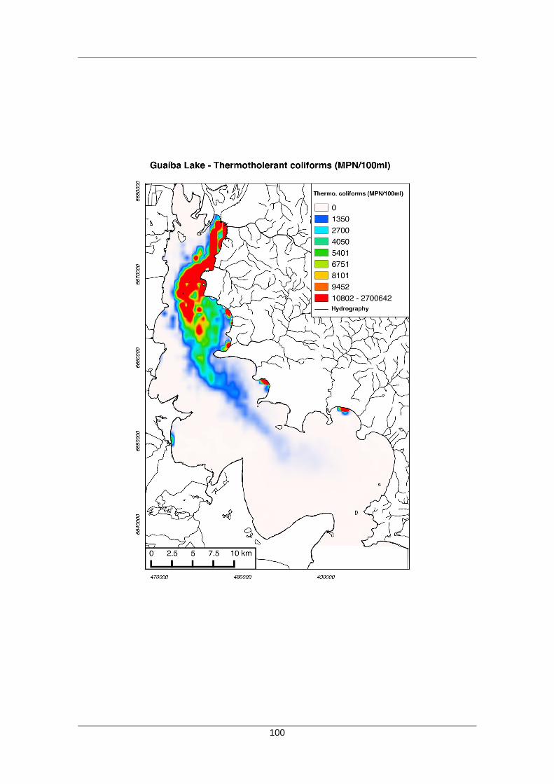
100

101

102
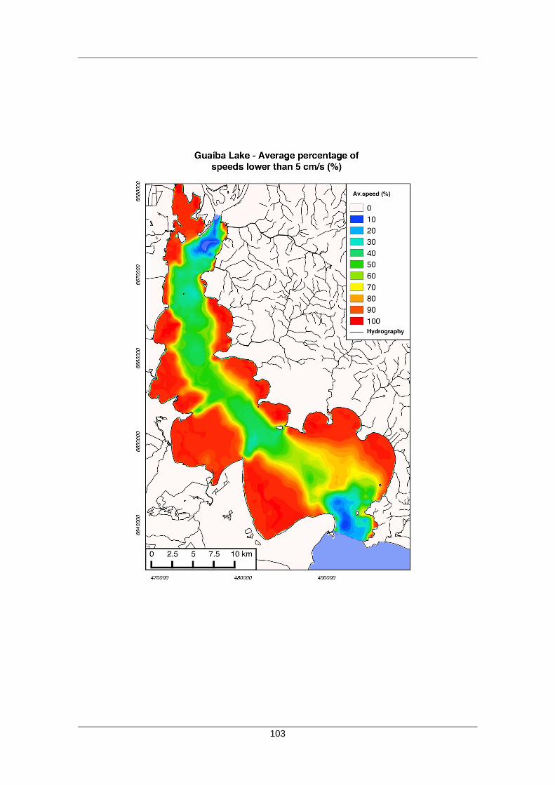
103

104
ANEXO 2: TABELA DE OCORRÊNCIAS DAS ESPÉCIES ANALIZADAS E PREDITORES

105
x y C. fluminea (ind/m2) L. anus P. nigribarbis P. pintado Pc.sand OM Depth Av.gran Season D.channel D.margin Het.gran NMP Speed.av
467478 6686346 4.4 0 0 0 97.131 1.002 2.8 0.231 sum 0.0 0.0 0.859 6.217 57.5
477823 6679509 30.8 5 7 3 61.048 14.801 1.5 0.627 sum 0.0 0.0 0.731 6.217 95.0
469137 6657724 26.4 0 0 5 98.948 0.341 1.5 0.735 sum 0.0 0.0 1.424 0.000 92.5
476790 6666481 0 1 0 9 91.858 3.114 2.3 0.627 aut 1100.2 60.0 1.549 6.909 92.5
474497 6658852 22 13 10 8 68.392 12.055 4 0.574 aut 4620.4 2313.1 0.785 6.909 47.5
476871 6676147 4.4 6 120 24 72.250 12.650 5.5 0.561 aut 480.9 234.3 0.832 9.210 82.5
473593 6683076 22 1 8 14 82.351 4.823 1.4 0.597 aut 0.0 0.0 0.682 2.398 12.5
469137 6657724 8.8 1 0 0 99.926 0.286 1.5 0.919 aut 0.0 0.0 1.423 0.000 92.5
472655 6666517 26.4 1 2 41 68.163 9.561 2.6 0.662 aut 2614.3 1273.5 0.726 6.909 35.0
487827 6642543 79.2 0 0 6 99.986 0.420 1.25 0.253 win 9991.0 1124.5 0.513 0.000 77.5
493487 6642625 105.6 6 0 33 96.203 2.783 2.6 0.227 win 5408.3 510.0 0.605 0.000 35.0
470995 6679649 57.2 1 0 7 90.353 3.547 1.6 0.364 win 582.5 134.2 0.568 0.000 92.5
477426 6662793 4.4 1 12 13 79.366 6.081 3.6 0.580 win 1348.3 174.9 0.749 6.217 95.0
497950 6648047 0 0 27 2 98.286 0.498 1.5 0.352 win 1263.2 67.1 1.103 0.000 95.0
468230 6686794 30.8 2 14 1 98.377 1.980 4.7 0.423 win 0.0 0.0 1.400 6.217 2.5
470050 6659043 4.4 10 40 7 99.570 3.480 2 0.631 spr 1677.1 566.0 1.535 6.909 95.0
475220 6672074 26.4 13 9 25 98.918 2.321 4.3 0.197 spr 934.3 706.1 0.777 8.517 40.0
478501 6654670 4.4 26 15 16 95.930 12.584 3.8 0.325 spr 5218.4 2885.6 1.053 6.217 42.5
497388 6650089 0 0 4 0 98.128 0.865 1.25 0.438 spr 218.4 150.0 1.287 0.000 95.0
495884 6646380 4.4 1 2 1 99.752 3.797 2.9 0.182 spr 2018.0 1043.6 0.749 0.000 87.5
476040 6652095 22 0 5 1 90.735 4.900 2.8 0.564 spr 5395.4 2747.6 1.028 0.000 92.5
476656 6645486 0 2 25 3 98.180 3.450 1.25 0.446 spr 863.8 182.5 1.352 0.000 92.5
485748 6647301 8.8 13 8 11 96.372 8.926 4 0.355 spr 7536.2 4243.2 1.171 2.398 70.0
477096 6683387 52.8 6 8 1 96.023 3.834 2.66 0.261 sum 0.0 0.0 0.485 4.615 65.0
470259 6670092 308 2 3 3 99.899 0.660 0.9 0.503 aut 391.2 30.0 1.456 2.398 97.5
474362 6688923 48.4 0 2 1 97.444 5.512 4.2 0.334 aut 0.0 0.0 0.921 6.217 5.0
472003 6655681 193.6 0 0 1 99.818 0.364 1.9 0.228 aut 3278.7 150.0 0.942 0.000 85.0
490581 6648770 17.6 2 0 13 98.680 9.944 3.6 0.353 aut 4905.8 3635.0 1.181 2.398 75.0
494774 6650794 4.4 0 0 5 94.451 0.914 2.9 0.398 aut 1783.2 300.0 1.186 0.000 95.0
484697 6651779 26.4 2 0 2 99.630 3.959 2.2 0.175 aut 2943.8 256.3 0.669 2.398 77.5
472253 6669981 30.8 1 0 5 99.045 10.450 4 0.598 aut 2229.9 1855.4 1.358 6.217 40.0
470029 6668140 35.2 0 3 1 99.834 0.632 1.5 0.250 win 1470.0 120.0 0.978 0.000 95.0

106
x y C. fluminea (ind/m2) L. anus P. nigribarbis P. pintado Pc.sand OM Depth Av.gran Season D.channel D.margin Het.gran NMP Speed.av
481392 6655452 4.4 0 0 0 99.777 1.014 3 0.838 win 2629.9 234.3 1.388 2.398 92.5
468830 6663407 0 0 4 4 96.313 3.780 1.75 0.505 win 0.0 0.0 1.404 6.217 95.0
470200 6673254 0 0 1 3 98.651 2.840 2.35 0.374 win 2153.5 30.0 1.253 2.398 95.0
473941 6668013 0 1 1 5 98.453 2.950 3.1 0.458 win 3702.7 815.0 1.395 6.217 32.5
483979 6644646 13.2 0 1 6 99.046 2.131 3.9 0.261 spr 8177.8 4039.4 1.099 0.000 93.5
473030 6647411 8.8 1 0 3 99.997 1.082 1.4 1.212 spr 3054.8 169.7 1.423 0.000 92.5
472104 6661456 1289.2 0 2 5 99.979 2.060 1.5 0.289 spr 3405.2 1726.8 1.011 2.398 55.0
481518 6684665 0 0 0 0 87.383 16.099 1.5 0.416 spr 0.0 0.0 0.777 13.816 100.0
477754 6665898 26.4 13 38 3 96.500 1.418 1.4 0.258 spr 123.7 67.1 0.690 13.816 67.5
475384 6675750 1650 4 2 3 97.489 1.740 0.7 0.211 spr 543.3 192.1 0.627 4.615 40.0
492717 6639658 246.4 2 8 6 100.000 0.247 3.5 0.268 sum 4388.8 1872.8 0.871 0.000 17.5
492274 6645440 202.4 1 29 16 99.870 0.470 2.9 0.256 sum 5741.0 3529.6 0.657 0.000 62.5
493435 6653352 4.4 0 4 0 98.858 1.688 1.8 0.583 sum 335.4 84.9 1.449 0.000 92.5
480209 6646740 140.8 0 6 6 99.441 0.440 2.3 0.314 sum 4649.5 450.0 0.802 0.000 92.5
480081 6649633 338.8 12 21 5 99.948 0.423 1.7 0.268 sum 6153.1 1426.2 0.629 0.000 52.5
476493 6672937 96.8 5 2 2 96.238 2.700 3 0.475 sum 846.9 84.9 1.467 6.909 72.5
474125 6673553 224.4 0 3 1 75.952 5.087 1.6 0.418 sum 2462.9 1320.0 0.598 4.615 17.5
477765 6660219 167.2 0 2 0 54.289 8.004 2.5 0.674 sum 1491.9 42.4 0.999 4.615 87.5
472605 6652095 52.8 1 0 3 99.646 1.192 1.8 0.565 sum 2696.7 499.3 1.539 2.398 92.5
475150 6654396 48.4 6 2 13 97.813 1.126 2.4 0.345 sum 6081.8 1667.1 1.017 0.000 62.5
476738 6657146 48.4 7 2 7 50.112 7.196 4 0.703 sum 4744.4 2973.8 0.625 6.909 52.5
469139 6655439 8.8 0 0 0 99.479 1.318 1.1 0.378 sum 2105.4 241.9 1.367 0.000 95.0