Embed Size (px)
Citation preview

POPULATION AND HEALTH IN
DEVELOPING COUNTRIES
V O L U M E 1


POPULATION AND HEALTH IN
DEVELOPING COUNTRIES
V O L U M E 1
Population, Health, and Survival
at INDEPTH Sites
INTERNATIONAL DEVELOPMENT RESEARCH CENTREOttawa • Cairo • Dakar • Montevideo • Nairobi • New Delhi • Singapore

Published by the International Development Research CentrePO Box 8500, Ottawa, ON, Canada K1G 3H9http://www.idrc.ca
© INDEPTH Network 2002
National Library of Canada cataloguing in publication data
Main entry under title :Population and health in developing countries. Volume 1. Population, health, and survival atINDEPTH sites
Includes bibliographical references.INDEPTH : International Network for the continuous Demographic Evaluation ofPopulations and their Health.ISBN 0-88936-948-8
1. Public health surveillance — Developing countries.2. Public health surveillance — Africa.3. Health planning — Developing countries.4. Public health — Developing countries — Statistics.5. Public health — Africa — Statistics.6. Developing countries — Population — Statistics.7. Health status indicators.I. INDEPTH Network.II. International Development Research Centre (Canada)
RA652.2.P82.P66 2001 614.4’22724 C2001-980345-1
All rights reserved. No part of this publication may be reproduced, stored in a retrieval system, or transmitted,in any form or by any means, electronic, mechanical, photocopying, or otherwise, without the prior permissionof the International Development Research Centre. Mention of a proprietary name does not constitute endorse-ment of the product and is given only for information.
IDRC Books endeavours to produce environmentally friendly publications. All paper used is recycled as wellas recyclable. All inks and coatings are vegetable-based products. The full catalogue of IDRC Books is availableat http://www.idrc.ca/booktique.

CONTENTS
Foreword . . . . . . . . . . . . . . . . . . . . . . . . . . . . . . . . . . . . . . . . . . . . . . . . . . . . . . . . . . . . . . . . . . .ixPreface . . . . . . . . . . . . . . . . . . . . . . . . . . . . . . . . . . . . . . . . . . . . . . . . . . . . . . . . . . . . . . . . . . . .xiAcknowledgments . . . . . . . . . . . . . . . . . . . . . . . . . . . . . . . . . . . . . . . . . . . . . . . . . . . . . . . . . .xiiiIntroduction . . . . . . . . . . . . . . . . . . . . . . . . . . . . . . . . . . . . . . . . . . . . . . . . . . . . . . . . . . . . . . . . .1
PART I. DSS CONCEPTS AND METHODS
Chapter 1. Core Concepts of DSS
Introduction . . . . . . . . . . . . . . . . . . . . . . . . . . . . . . . . . . . . . . . . . . . . . . . . . . . . . . . . . . . . . . . .7Demographic surveillance systems . . . . . . . . . . . . . . . . . . . . . . . . . . . . . . . . . . . . . . . . . . . . . .7Demographic surveillance area . . . . . . . . . . . . . . . . . . . . . . . . . . . . . . . . . . . . . . . . . . . . . . . . .8Longitudinality . . . . . . . . . . . . . . . . . . . . . . . . . . . . . . . . . . . . . . . . . . . . . . . . . . . . . . . . . . . . . .8Primary DSS subjects . . . . . . . . . . . . . . . . . . . . . . . . . . . . . . . . . . . . . . . . . . . . . . . . . . . . . . . . .9Eligibility . . . . . . . . . . . . . . . . . . . . . . . . . . . . . . . . . . . . . . . . . . . . . . . . . . . . . . . . . . . . . . . . . .11Residency and membership . . . . . . . . . . . . . . . . . . . . . . . . . . . . . . . . . . . . . . . . . . . . . . . . . . .12Core DSS events . . . . . . . . . . . . . . . . . . . . . . . . . . . . . . . . . . . . . . . . . . . . . . . . . . . . . . . . . . . .12Episodes . . . . . . . . . . . . . . . . . . . . . . . . . . . . . . . . . . . . . . . . . . . . . . . . . . . . . . . . . . . . . . . . . .14Other events . . . . . . . . . . . . . . . . . . . . . . . . . . . . . . . . . . . . . . . . . . . . . . . . . . . . . . . . . . . . . . .15
Chapter 2. DSS-generated Mortality Rates and Measures
Introduction . . . . . . . . . . . . . . . . . . . . . . . . . . . . . . . . . . . . . . . . . . . . . . . . . . . . . . . . . . . . . . .17Rates and ratios . . . . . . . . . . . . . . . . . . . . . . . . . . . . . . . . . . . . . . . . . . . . . . . . . . . . . . . . . . . . .17Standardization . . . . . . . . . . . . . . . . . . . . . . . . . . . . . . . . . . . . . . . . . . . . . . . . . . . . . . . . . . . . .20Confidence intervals for rates . . . . . . . . . . . . . . . . . . . . . . . . . . . . . . . . . . . . . . . . . . . . . . . . .20
Chapter 3. DSS Methods of Data Collection
Introduction . . . . . . . . . . . . . . . . . . . . . . . . . . . . . . . . . . . . . . . . . . . . . . . . . . . . . . . . . . . . . . .21Establishing the monitored population . . . . . . . . . . . . . . . . . . . . . . . . . . . . . . . . . . . . . . . . .22Planning for data collection . . . . . . . . . . . . . . . . . . . . . . . . . . . . . . . . . . . . . . . . . . . . . . . . . .23Initial census . . . . . . . . . . . . . . . . . . . . . . . . . . . . . . . . . . . . . . . . . . . . . . . . . . . . . . . . . . . . . . .23Update rounds . . . . . . . . . . . . . . . . . . . . . . . . . . . . . . . . . . . . . . . . . . . . . . . . . . . . . . . . . . . . .23Recording demographic events . . . . . . . . . . . . . . . . . . . . . . . . . . . . . . . . . . . . . . . . . . . . . . . .26Monitoring mortality . . . . . . . . . . . . . . . . . . . . . . . . . . . . . . . . . . . . . . . . . . . . . . . . . . . . . . . .27Tracking migrants . . . . . . . . . . . . . . . . . . . . . . . . . . . . . . . . . . . . . . . . . . . . . . . . . . . . . . . . . .28
v

Additional rounds of data collection . . . . . . . . . . . . . . . . . . . . . . . . . . . . . . . . . . . . . . . . . . . .29Geographic information systems . . . . . . . . . . . . . . . . . . . . . . . . . . . . . . . . . . . . . . . . . . . . . . .29Conclusion . . . . . . . . . . . . . . . . . . . . . . . . . . . . . . . . . . . . . . . . . . . . . . . . . . . . . . . . . . . . . . . .30
Chapter 4. Processing DSS Data
Introduction . . . . . . . . . . . . . . . . . . . . . . . . . . . . . . . . . . . . . . . . . . . . . . . . . . . . . . . . . . . . . . .31Background . . . . . . . . . . . . . . . . . . . . . . . . . . . . . . . . . . . . . . . . . . . . . . . . . . . . . . . . . . . . . . .32The INDEPTH concept of a data core . . . . . . . . . . . . . . . . . . . . . . . . . . . . . . . . . . . . . . . . . .33The reference data model . . . . . . . . . . . . . . . . . . . . . . . . . . . . . . . . . . . . . . . . . . . . . . . . . . . .35The role of the reference data model in maintaining data integrity . . . . . . . . . . . . . . . . . .39Extending the core . . . . . . . . . . . . . . . . . . . . . . . . . . . . . . . . . . . . . . . . . . . . . . . . . . . . . . . . . .40Conclusion . . . . . . . . . . . . . . . . . . . . . . . . . . . . . . . . . . . . . . . . . . . . . . . . . . . . . . . . . . . . . . .41
Chapter 5. Assessing the Quality of DSS Data
Introduction . . . . . . . . . . . . . . . . . . . . . . . . . . . . . . . . . . . . . . . . . . . . . . . . . . . . . . . . . . . . . . .43Assessing data quality in the field . . . . . . . . . . . . . . . . . . . . . . . . . . . . . . . . . . . . . . . . . . . . . .43Assessing data quality at the data centre . . . . . . . . . . . . . . . . . . . . . . . . . . . . . . . . . . . . . . . . .44Conclusion . . . . . . . . . . . . . . . . . . . . . . . . . . . . . . . . . . . . . . . . . . . . . . . . . . . . . . . . . . . . . . .47
PART II. MORTALITY AT INDEPTH SITES
Chapter 6. Comparing Mortality Patterns at INDEPTH Sites
Abstract . . . . . . . . . . . . . . . . . . . . . . . . . . . . . . . . . . . . . . . . . . . . . . . . . . . . . . . . . . . . . . . . . . .51Introduction . . . . . . . . . . . . . . . . . . . . . . . . . . . . . . . . . . . . . . . . . . . . . . . . . . . . . . . . . . . . . . .51Age-specific mortality rates and life tables . . . . . . . . . . . . . . . . . . . . . . . . . . . . . . . . . . . . . . .52Crude death rate . . . . . . . . . . . . . . . . . . . . . . . . . . . . . . . . . . . . . . . . . . . . . . . . . . . . . . . . . . . .53Child mortality . . . . . . . . . . . . . . . . . . . . . . . . . . . . . . . . . . . . . . . . . . . . . . . . . . . . . . . . . . . . .57Adult mortality . . . . . . . . . . . . . . . . . . . . . . . . . . . . . . . . . . . . . . . . . . . . . . . . . . . . . . . . . . . . .59Discussion . . . . . . . . . . . . . . . . . . . . . . . . . . . . . . . . . . . . . . . . . . . . . . . . . . . . . . . . . . . . . . . . .61Annex: Life tables . . . . . . . . . . . . . . . . . . . . . . . . . . . . . . . . . . . . . . . . . . . . . . . . . . . . . . . . . . .63
Chapter 7. INDEPTH Mortality Patterns for Africa
Abstract . . . . . . . . . . . . . . . . . . . . . . . . . . . . . . . . . . . . . . . . . . . . . . . . . . . . . . . . . . . . . . . . . . .83Mortality models and Africa . . . . . . . . . . . . . . . . . . . . . . . . . . . . . . . . . . . . . . . . . . . . . . . . . . .83Principal-components analysis . . . . . . . . . . . . . . . . . . . . . . . . . . . . . . . . . . . . . . . . . . . . . . . . .87Principal components of INDEPTH mortality data . . . . . . . . . . . . . . . . . . . . . . . . . . . . . . . .89INDEPTH mortality patterns . . . . . . . . . . . . . . . . . . . . . . . . . . . . . . . . . . . . . . . . . . . . . . . . . .96Demonstration of the HIV–AIDS model life-table system . . . . . . . . . . . . . . . . . . . . . . . . . .111Conclusion . . . . . . . . . . . . . . . . . . . . . . . . . . . . . . . . . . . . . . . . . . . . . . . . . . . . . . . . . . . . . . .114Annex: AIDS-decremented model life tables . . . . . . . . . . . . . . . . . . . . . . . . . . . . . . . . . . . .115
vi ✦ Contents
PART III. INDEPTH DSS SITE PROFILES
Introduction . . . . . . . . . . . . . . . . . . . . . . . . . . . . . . . . . . . . . . . . . . . . . . . . . . . . . . . . . . . . . .129
Chapter 8. Butajira DSS, Ethiopia . . . . . . . . . . . . . . . . . . . . . . . . . . . . . . . . . . . . . . . . . . . .135
Chapter 9. Dar es Salaam DSS, Tanzania . . . . . . . . . . . . . . . . . . . . . . . . . . . . . . . . . . . . . .143
Chapter 10. Hai DSS, Tanzania . . . . . . . . . . . . . . . . . . . . . . . . . . . . . . . . . . . . . . . . . . . . . . .151
Chapter 11. Ifakara DSS, Tanzania . . . . . . . . . . . . . . . . . . . . . . . . . . . . . . . . . . . . . . . . . . . .159
Chapter 12. Morogoro DSS, Tanzania . . . . . . . . . . . . . . . . . . . . . . . . . . . . . . . . . . . . . . . . . .165
Chapter 13. Rufiji DSS, Tanzania . . . . . . . . . . . . . . . . . . . . . . . . . . . . . . . . . . . . . . . . . . . . .173
Chapter 14. Gwembe DSS, Zambia . . . . . . . . . . . . . . . . . . . . . . . . . . . . . . . . . . . . . . . . . . . .183
Chapter 15. Manhiça DSS, Mozambique . . . . . . . . . . . . . . . . . . . . . . . . . . . . . . . . . . . . . . .189
Chapter 16. Agincourt DSS, South Africa . . . . . . . . . . . . . . . . . . . . . . . . . . . . . . . . . . . . . . .197
Chapter 17. Dikgale DSS, South Africa . . . . . . . . . . . . . . . . . . . . . . . . . . . . . . . . . . . . . . . . .207
Chapter 18. Hlabisa DSS, South Africa . . . . . . . . . . . . . . . . . . . . . . . . . . . . . . . . . . . . . . . . .213
Chapter 19. Nouna DSS, Burkina Faso . . . . . . . . . . . . . . . . . . . . . . . . . . . . . . . . . . . . . . . . .221
Chapter 20. Oubritenga DSS, Burkina Faso . . . . . . . . . . . . . . . . . . . . . . . . . . . . . . . . . . . . .227
Chapter 21. Farafenni DSS, The Gambia . . . . . . . . . . . . . . . . . . . . . . . . . . . . . . . . . . . . . . . .235
Chapter 22. Navrongo DSS, Ghana . . . . . . . . . . . . . . . . . . . . . . . . . . . . . . . . . . . . . . . . . . . .247
Chapter 23. Bandim DSS, Guinea-Bissau . . . . . . . . . . . . . . . . . . . . . . . . . . . . . . . . . . . . . . .257
Chapter 24. Bandafassi DSS, Senegal . . . . . . . . . . . . . . . . . . . . . . . . . . . . . . . . . . . . . . . . .263
Chapter 25. Mlomp DSS, Senegal . . . . . . . . . . . . . . . . . . . . . . . . . . . . . . . . . . . . . . . . . . . . .271
Chapter 26. Niakhar DSS, Senegal . . . . . . . . . . . . . . . . . . . . . . . . . . . . . . . . . . . . . . . . . . . .279
Chapter 27. Matlab DSS, Bangladesh . . . . . . . . . . . . . . . . . . . . . . . . . . . . . . . . . . . . . . . . .287
Chapter 28. ORP DSS, Bangladesh . . . . . . . . . . . . . . . . . . . . . . . . . . . . . . . . . . . . . . . . . . . .297
Chapter 29. FilaBavi DSS, Viet Nam . . . . . . . . . . . . . . . . . . . . . . . . . . . . . . . . . . . . . . . . . . .305
Contents ✦ vii

viii ✦ Contents
Appendix 1. Working Examples of DSS Forms
Example 1. DSS Baseline Form (Rufiji DSS) . . . . . . . . . . . . . . . . . . . . . . . . . . . . . . . . . . .312Example 2. Household Registration Book (HRB) (Rufiji DSS) . . . . . . . . . . . . . . . . . . . .313Example 3. Pregnancy Outcome / Birth Form (Rufiji DSS) . . . . . . . . . . . . . . . . . . . . . . .315Example 4. Death Registration Form (Navrongo DSS) . . . . . . . . . . . . . . . . . . . . . . . . . . .316Example 5. Marital Status Form (Butajira DSS) . . . . . . . . . . . . . . . . . . . . . . . . . . . . . . . . .316Example 6. VA Form: Deaths of Children from Day 31 to 5 Years (Morogoro DSS) . . . .318Example 7. In-migration Form (Navrongo DSS) . . . . . . . . . . . . . . . . . . . . . . . . . . . . . . . .320Example 8. Out-migration Form (Navrongo DSS) . . . . . . . . . . . . . . . . . . . . . . . . . . . . . . .321
Appendix 2. Acronyms and Abbreviations . . . . . . . . . . . . . . . . . . . . . . . . . . . . . . . . . . . . . . .323
Appendix 3. Glossary . . . . . . . . . . . . . . . . . . . . . . . . . . . . . . . . . . . . . . . . . . . . . . . . . . . . . . .327
Appendix 4. Bibliography . . . . . . . . . . . . . . . . . . . . . . . . . . . . . . . . . . . . . . . . . . . . . . . . . . .333

ix
FOREWORD
Traditional sources of health information collected from health facilities often serve asthe basis for health-services planning and allocation of resources in many parts of thedeveloping world. Yet, health-facility-based data provide only fragmentary and biasedinformation. Not all population groups have geographic or economic access to healthfacilities. Those that do have such access are usually self-selected and are often thosewho visit health-care centres only when they suffer from a serious illness. A greatmajority of poor people may have less access to health-care facilities than those whoare better off, and poor people often treat themselves or use nontraditional healthcare. Women may suffer gender disparities as well, with time and cultural constraintson the use of health-care facilities, particularly in rural settings. Services for childrenare also severely constrained. Thus, health-facility-based data are not representative ofthe health problems of all rural and urban communities and do not therefore reflecttheir health status.
This void of valid health information for a large segment of the world’s popula-tion makes it difficult for policymakers to formulate rational health policies toimprove the health of these people. As the authors of this book argue, “the need toestablish a reliable information base to support health development has never beengreater” (INDEPTH Coordinating Committee, this volume, p. 1). Ideally, reliablehealth information should be population and community based, inclusive of allgroups, and collected prospectively and continuously. Such an ideal is best metthrough demographic and health surveillance systems collecting demographic andhealth data on selected population samples. Often, randomly selected cross-sectionalhousehold surveys every few years complement these methods of research.
Demographic and health surveillance systems serve a number of functions:
• They provide health information that more accurately reflects the prevailingdisease burden of populations;
• They assist in monitoring and tracking new health threats, such as emergingand reemerging infectious disease and drug resistance, and alert the healthcommunity to prepare a response; and
• They can serve as a platform for action-oriented research to test and evaluatehealth interventions, such as new vaccines or drugs, health-education messages,and the cost-effectiveness of initiatives.
The premier example of such a system is the Health and DemographicSurveillance System (formerly known as the Demographic Surveillance System) ofMatlab, Bangladesh, which started operations in 1963 as a major component of the

x ✦ Foreword
field research program of the International Centre for Diarrhoeal Disease Research,Bangladesh. It is recognized as the largest and longest sustained prospective longitudi-nal demographic and health surveillance of any population in the world. It has madesignificant contributions to health development in both Bangladesh and the rest ofthe world. The high cost of running such a system has delayed replication in otherparts of the developing world. However, thanks to the fast-paced development of user-friendly computers, this constraint has been partially overcome.
Over the last decade, a growing number of community-based field stations haveevolved in Asia and sub-Saharan Africa and started to generate reliable longitudinalpopulation-based health and demographic data. This bodes well for countries withsuch stations, as it marks the first step toward rational health planning and meaningfulhealth programs for the people of these countries. Recently, these stations joined toform a network called the International Network for the continuous DemographicEvaluation of Populations and Their Health in developing countries (INDEPTH), cre-ating “a trans-continental resource of robust, longitudinal, health and demographicdata in some of the most information deprived settings in the world” (INDEPTHFounding Document; http://www.indepth-network.org). In the span of a few years,INDEPTH has matured rapidly, succeeding in strengthening the capabilities of mem-ber sites and developing strategies to harness their potential to redress long-standinginequities in health. This development has been possible because of the dedicationand hard work of a few individuals, and this monograph is clearly an indication of thehigh quality of the network’s work.
The emergence of INDEPTH should be welcome news to the donor commu-nity, where people often, and rightly, complain that the programs they fund in low-income countries are not usually based on the real needs of the people. By the sametoken, donors should come out strongly in support of INDEPTH, because they will beinvesting in an initiative that directly addresses one of the major constraints of devel-opment assistance. Researchers in program countries should also take advantage ofthe INDEPTH sites to promote essential national health research. The domination ofhealth-facility-based biomedical research should give way to policy-relevant researchwith the likelihood of a more immediate effect on the health of the people in thecountries in the program.
Demissie HabteWorld BankWashington, DC1 June 2001

PREFACE
This monograph is the first in a series from the International Network for the continu-ous Demographic Evaluation of Populations and Their Health in developing countries(INDEPTH). It seeks to do several things. First, it seeks to compile, for both easy refer-ence and comparative purposes, and in detailed and summary formats, the essentialcharacteristics of each participating demographic surveillance system (DSS) site.Second, it seeks to present, for the first time, the mortality structure of each of thesesites in a coherent and comparative format. Third, based on a network-wide analysis ofthe African site data, it proposes a methodology to generate, again for the first time,African model life tables that are based on objective empirical data.
The focus of this volume is the structures of populations at INDEPTH sites andthe characteristics of their health and survival. The monograph is divided into threeparts: Part I discusses core concepts and methods used in DSSs; Part II provides a com-parison of mortality patterns in INDEPTH sites; and Part III presents profiles ofINDEPTH sites.
As this is the first publication of its kind on DSSs in Africa and Asia, we thoughtit would be expedient to discuss core concepts and methods commonly used in mostof the sites. Among the concepts discussed in Chapter 1 are the DSS area, longitudi-nality, DSS subjects, residency and membership, and core DSS events. Rates and mea-sures generated using DSS are discussed in Chapter 2, with specific emphasis on theuse of person–years lived in calculating rates. Chapter 3 discusses the DSS methods ofdata collection, starting with the initial census to establish the DSS population. Thischapter discusses initial censuses, update rounds, and the vital events-registration sys-tem. It also puts emphasis on mortality monitoring and the tracking of migrants. Theprocessing of DSS data is the main focus of Chapter 4. This chapter treats the impor-tant issues of quality assurance and control at the data-processing level. In Chapter 5,Part I ends with a discussion of the quality of DSS data, both in the field and at thedata centre. This chapter then provides a detailed discussion of statistical and demo-graphic techniques for analysis of DSS data.
Part II presents a comparison of mortality patterns of INDEPTH sites for the1995–99 period. Chapter 6 starts with a discussion of crude overall mortality atINDEPTH sites. This chapter presents an INDEPTH population-age standard for sub-Saharan Africa (SSA) for the standardization of mortality rates, and it gives the reasonfor using this new standard instead of the United Nations models.
The INDEPTH age standard for SSA typifies the population in developingcountries, with its very young age structure. INDEPTH sites have used this standard tocompare mortality in SSA. This comparison highlights age-specific mortality, consider-ing mortality in infancy, childhood, and adulthood. This discussion compares theINDEPTH standard for SSA with the Segi population and the new World Health
xi

xii ✦ Preface
Organization standard population. The chapter ends with a presentation of basic life-table indicators for INDEPTH sites, based on their age-specific mortality rates over the1995–99 period. Part II ends with Chapter 7, which analyzes more than 6.4 millionperson–years of observation at the African INDEPTH sites to identify mortality pat-terns. The emergent patterns are demonstrated to be substantially different from con-ventionally used model mortality patterns applied in Africa.
Part III presents profiles of 22 INDEPTH sites. The profiles are listed in alpha-betical order, first according to region, and then according to country. These profilesare expected to stand for some time as the main reference source for basic detailsabout INDEPTH sites and their DSS operations. Based on a structured template, eachprofile provides a site description, including the physical geography and populationcharacteristics. It discusses DSS procedures at the site, including data collection andprocessing. Finally, each profile presents basic outputs, including demographic indica-tors. A summary matrix of all the DSS sites, presented in the introduction to Part III,provides the core details for each site.
INDEPTH monograph editorial team for Volume 1:
Osman A. Sankoh (University of Heidelberg, Germany, and Nouna DSS,Burkina Faso)
Kathleen Kahn (Agincourt DSS, South Africa)Eleuther Mwageni (Rufiji DSS, Tanzania)Pierre Ngom (Nairobi DSS, Kenya)Philomena Nyarko (Navrongo DSS, Ghana)
1 June 2001
ACKNOWLEDGMENTS
This volume is an outgrowth of the efforts of many people, both INDEPTH membersand its collaborators, who gave of their time and expertise to writing these chapters.We would like to particularly thank the following for their invaluable contributions tothe corresponding chapters:
• Pierre Ngom, Justus Benzler, Geoff Solarsh, and Vicky Hosegood (Chapter 1);
• Rose Nathan, Heiko Becher, and Abdur Razzaque (Chapter 2);
• Eleuther Mwageni and Robert Mswia (Chapter 3);
• Peter Wontuo, Noah Kiwanuka, and Jim Phillips (Chapter 4)1;
• Philomena Nyarko, Fred Binka, and Mark Collinson (Chapter 5);
• Sam Clark and Pierre Ngom (Chapter 6);
• Sam Clark (Chapter 7); and
• DSS site teams (Chapters 8–29).
We would also like to thank INDEPTH site members, whose names are men-tioned in the site profiles, for coordinating the writing of their site’s profile. Specialthanks go to Rose Lusinde and Don de Savigny for producing the map panels for thesite locations and particularly to Kathleen Kahn and Don de Savigny for coordinatingthe formatting and editing of the 22 site-profile chapters making up Part III of themonograph.
The INDEPTH coordinators would like to express their gratitude to theINDEPTH editorial committee, led by Osman A. Sankoh, for its outstanding work incompiling this first monograph. We acknowledge with pleasure the willingness of indi-vidual site teams and their leaders to collaborate in sharing such rich data sets andexperiences. We also recognize the contributions of all our investment partners —local communities, public-sector services, academic and research institutions, anddonors — all of whom, often over prolonged periods, continue to support and sustainour efforts. We express particular thanks and appreciation to the many sponsors ofINDEPTH, including the Rockefeller Foundation, the Navrongo Health ResearchCentre, the Population Council, the World Health Organization, and the Andrew W.
xiii
1 Based on Benzler, J.; Herbst, A.J.; MacLeod, B. (in alphabetical order): A reference data model for demographic surveillance systems.INDEPTH 1999, http://www.indepth-network.org.

xiv ✦ Acknowledgements
Mellon Foundation, for providing the funds needed to enable INDEPTH networkingactivities to function. We look forward to attracting new partners to join with us inadvancing our mission, goals, activities, and products.
Finally, we thank internal and external reviewers for their invaluable com-ments, which increased the validity and clarity of many sections of the monograph.
INDEPTH Coordinating Committee
Fred Binka, Chair (Ghana, 1998–2001)Steve Tollman, Deputy Chair (South Africa, 1998–2001)Pedro Alonso, Member (Mozambique, 1998–2000)Yemane Berhane, Member (Ethiopia, 1998–2001)Chuc N.T.K., Member (Viet Nam, 2000–)Don de Savigny, Member (Tanzania, 1998–2001)Bocar Kouyaté, Member (Burkina Faso, 2000–)Boubakar Sow, Member (Mali, 1998–1999) Siswanto Wilopo, Member (Indonesia, 1998–2001)
1 June 2001

INTRODUCTION
As we enter the new millennium, with the revolution of the information age still gain-ing speed, it seems inconceivable that large parts of the Earth’s population remaindevoid of vital health information. For 1 billion people living in the world’s poorestcountries, where the burden of disease is highest, no one registers those who are bornor who die or ascertains the causes of their deaths. From the limited data available, thehealth profile of these populations can be likened to an iceberg: the bulk of reliabledata on trends in age, gender, geographic variations, and burden of disease remainshidden. This great void in population-based information constitutes a major and long-standing constraint on the articulation of effective policies and programs to improvethe health of the poor and thus perpetuates profound inequities in health. The needto establish a reliable information base to support health development has never beengreater.
Recently, experience has emerged from a growing number of community-basedfield stations that have continuous monitoring systems for geographically defined pop-ulations. These field stations generate high-quality, population-based, longitudinalhealth and demographic data with the potential to fill this information void in thedeveloping world. Since 1997 a number of organizations have made a systematic effortto harness and make more readily available the products of these disparate initiatives.A series of meetings were convened by the University of Witwatersrand (South Africa)(Agincourt Health and Population Programme); Department of Tropical Hygiene andPublic Health, University of Heidelberg (Germany); the Rockefeller Foundation(Bellagio, Italy); and the Ministry of Health (Navrongo, Ghana) to examine the poten-tial for harnessing these sites through a network. These activities culminated in ameeting convened in Dar es Salaam, Tanzania, 9–12 November 1998, to establish sucha network.
Seventeen field sites drawn from 13 countries in Africa and Asia participated inthis founding meeting. The name adopted for the network was the InternationalNetwork for the continuous Demographic Evaluation of Populations and Their Healthin developing countries (INDEPTH). Network membership has increased steadilysince then and currently stands at 29 health and demographic evaluation sites in16 countries (the 13 countries whose sites are profiled in this volume are shown inFigure I.1). The network’s founding document and constitution are available on theINDEPTH website (www.INDEPTH-network.org).
1

Figure I.1 Countries with DSS field sites participating in the INDEPTH network.
The defining characteristics of an INDEPTH field site are the following:
• A geographically defined population is under continuous demographic moni-toring, with timely production of data on all births, deaths, and migrations —sometimes called a demographic surveillance system (DSS); and
• This monitoring system provides a platform for a wide range of health-systeminnovations, as well as social, economic, behavioural, and health interventions,all closely associated with research activities.
The vision and goals of the network are
• To enhance substantially the capabilities of INDEPTH sites through technicalstrengthening, methodological development, widened applications to policyand practice, and increased interaction of site leaders, researchers, and man-agers; and thus
• To realize their potential to generate the information needed to– Set health priorities,– Allocate resources more efficiently and equitably,– Inform the development, implementation, and evaluation of health inter-
ventions and other social-sector programs,– Strengthen the decision-making capability of information systems,– Define a highly relevant research and development agenda,– Augment national research capacity, and thereby– Fulfill developing-country potential to redress long-standing inequities in
health.
2 ✦ Introduction

To achieve these goals and facilitate the effective interaction of INDEPTH sites,the network has identified the concept of flexible working groups focused on specificscientific issues or topics as a key mechanism. Seven working groups were initiallyestablished, with a focus on
• Comparative assessments of mortality;
• Analysis and capacity-strengthening;
• Technical support for field sites;
• Reproductive health;
• Malaria;
• Information and publications; or
• Applications to policy and practice.
Two further working groups have since been formed, focusing on adult healthand ethical practice. Thus, through active and concerted efforts, the network is encom-passing a critical agenda founded on traditional strengths in research on infectiousdiseases and nutrition, with a growing emphasis on reproductive health, and the net-work is extending this emphasis to chronic disease, injury, and related social phenom-ena such as rapid urbanization. A central objective is to use network sites to train localscientists in research and research management.
This monograph is the foundation for an INDEPTH series on various themes,including model life tables for Africa and Asia; cause-specific mortality in developingcountries; migration patterns; trends in fertility; reproductive health (includingHIV–AIDS); and health equity.
INDEPTH Coordinating CommitteeAccra, GhanaJune 2001
Introduction ✦ 3


P A R T I
DSS CONCEPTS AND METHODS


Chapter 1
CORE CONCEPTS OF DSS
Introduction
During the past 30 years, demographic surveillance systems (DSSs) have been estab-lished in a number of field research sites in various parts of the developing worldwhere routine vital-registration systems were poorly developed or nonexistent.Although these systems may have been developed differently in terms of their initialrationale, they are all required to track a limited and common set of key variablesdetermining population dynamics and demographic trends. DSSs have similarapproaches to defining key variables and their relationships and to developing systemsfor collection, storage, and analysis of these data. The core concepts presented heredraw directly from the ideas and experiences emerging from INDEPTH DSS sites inAfrica and Asia. It should be emphasized, however, that even though an effort hasbeen made to standardize the definitions, many DSS sites still define some of the con-cepts differently.
Demographic surveillance systems
A DSS is a set of field and computing operations to handle the longitudinal follow-upof well-defined entities or primary subjects (individuals, households, and residentialunits) and all related demographic and health outcomes within a clearly circum-scribed geographic area. Unlike a cohort study, a DSS follows up the entire populationof such a geographic area.
In such a system, an initial census defines and registers the target population.Regular subsequent rounds of data collection at prescribed intervals make it possibleto register all new individuals, households, and residential units and to update keyvariables and attributes of existing subjects. The core system provides for monitoringof population dynamics through routine collection and processing of information onbirths, deaths, and migrations — the only demographic events leading to any changein the initial size of the resident population. This core system is often complementedby various other data sets that provide important social and economic correlates ofpopulation and health dynamics. These may include information on events such ashousehold formation and dissolution, acquisition and loss of economic assets, andgrowth or depletion of income.
7

8 ✦ DSS Concepts and Methods
In many population sites, the DSS may also provide a platform for other studieswithin the same geographic area. This support varies from one study to another andmay include the provision of an initial sampling frame, adjustment for confoundingvariables, provision of additional explanatory variables, and measurement of thedemographic impact of interventions.
Demographic surveillance area
The demographic surveillance area (DSA) is an area with clearly and fairly permanentdelineated boundaries, preferably recognizable on the ground (for example, rivers,roads, and clearly demarcated administrative boundaries). The clear delineation ofboundaries enables an unambiguous distinction to be made between individuals,households, and residential units to include in the DSS and those to exclude.
The area of a DSS site depends mainly on the size of the population requiredfor demographic surveillance and related research activities (for a typical example, see“Establishing the monitored population” in Chapter 3). The size is also influenced bypragmatic considerations, such as the cost to the research centre and its capacity tomanage the associated logistics and human resources. The DSA may expand or shrinkover time in response to changing research needs or sources of funding. Thesechanges usually introduce additional complexity, as they alter eligibility criteria andmay make it difficult to maintain consistent definitions of internal and external migra-tions over the period of transition.
Longitudinality
Longitudinal measurement of demographic and health variables is one of the keycharacteristics of a DSS. This is achieved through repeated visits at more or less regu-lar intervals to all residential units in the DSA to collect a prescribed set of attributedata on registered subjects, who are consistently and uniquely identified. This andrecording events affecting these subjects during the interval between visits allow one toconstruct their history and differentiate DSS data from data collected in multiroundsurveys and other prospective studies that allow comparison over time only on anaggregated level.
Visits
DSSs collect data during rounds, or cycles, of visits to registered residential units in theDSA. The interval between visits depends on the frequency of the changes in the phe-nomena under study and on the length of recall intervals for the collected data, andthus on the research focus of each field site. However, like the size of the DSA andobserved population, it also depends on funding and logistics. This interval variesfrom one site to another, ranging from 1 week to 1 year. However, for the majority ofDSSs, observations are made at 3- or 4-month intervals. This is widely considered anappropriate interval to ensure comprehensive recording of births, deaths, and migra-tions, which is the minimum requirement for maintaining the coherence of any DSS .

Core Concepts of DSS ✦ 9
When intervals between visits are long (a year or more), researchers commonlyignore migration events and instead conduct a full census at each new round. In- andout-migration flows are then inferred through reconciliation of unlinked censusrecords after account is taken of births and deaths between censuses.
Data collected during each fieldwork round are not restricted to key demo-graphic events but may also include the various attributes of the primary subjects.These attributes may be fixed (for example, ethnicity, gender) or changing over time(for example, marital or residential status).
Unique identifiers
Unique identifiers for primary subjects are an indispensable element of DSSs. All sys-tems invariably formulate rules for assigning unique identifiers at the start of the DSS,but their methods for assigning these identifiers to DSS subjects may vary from onesite to another. There are two main approaches. One common strategy is to transpar-ently link the subjects in a single residential unit through a hierarchical system ofunique numbers. These are built up from a unique number for the residential unit,followed by serial numbers for each of the households within it (where the notion ofhouseholds applies) and then for each of the enumerated individuals within eachhousehold. In this system, the unique number for each individual in the DSS is a com-posite of the numbers for the residential unit, household, and household member.This may involve creating complex hierarchies, in which the unique number of theresidential unit itself is a composite reflecting allocation to regions, areas, and villages(where they exist). This system requires thorough mapping of the DSA beforeenumeration. It also requires proper training of enumerators to avoid confusion inassigning identifiers. When mapping of the DSA is coupled with georeferencing of res-idential units, using geographic information system (GIS) technology, global position-ing system (GPS) coordinates are assigned as location attributes of the residentialunits within the database.
The other strategy for assigning identifiers to individuals is to avoid any fixedlink to residential units and households. In this system, identifiers for each subject aresimply serial numbers incremented each time a new DSS subject is registered. This sys-tem requires providing field staff with block allocations of ID numbers with enoughlatitude to register new subjects. This approach should be coupled with computergeneration of the identifiers to safeguard against the assignment of the same ID to mul-tiple subjects on the ground. This strategy helps to preserve people’s anonymity outsidetheir residential units, or when their attribute data are accessed through the database.
Primary DSS subjects
DSSs are typically structured around three main subjects (Figure 1.1) within the DSA.These subjects have both a conceptual and a logistical rationale. From a logisticalpoint of view, it is not feasible to interview all individuals directly, and for this reasonindividuals are put in groups with physical and social meaning, and information is col-lected from credible and informed respondents within these groups. The reasons todistinguish between these subjects from a conceptual point of view will be dealt with ingreater detail in the following subsections. The three main subjects are (Figure 1.1) asfollows:

Figure 1.1. The three main DSS subjects.
• Residential units — These are the places where individuals live. They are definedin physical and geographic terms.
• Households — These are the groups to which individual members belong. Theyare often defined as social subunits of the residential unit.
• Individuals — These are the people who are living in the residential units andhouseholds. They are the subject of main interest in any DSS.
Residential units
All DSSs identify residential units as a primary subject of interest, although they vary inthe terms they use for these units (for example, compounds or homesteads) and may alsodiffer slightly in their definition of them. Residency, or physical presence within a DSAat a fixed place of abode and for a sufficiently long period, is an essential prerequisitefor the enumeration of individuals at risk for demographic events or disease exposure.
In most systems a distinction is made between places of residence and otherstructures, such as clinics, schools, churches, and stores. Identifying a unifying termfor all these structural units may have conceptual merit, and some systems haveattempted to do this, as these structural units share many characteristics and thisapproach simplifies the database hierarchy for handling this concept. In this system aninclusive term such as bounded structure may be used at a higher level and compounds(or homesteads) and facilities at the more specific level.
Households
Households may be variably defined in one or more of the following ways:
• A group of people who consume or make some contribution to food and othershared resources;
10 ✦ DSS Concepts and Methods
Residential Unit
part of / resident at resident at
member ofHousehold Individual

• A group of people who have a common allegiance to an acknowledged head ofa household;
• A group of people, each of whom is recognized by other members of the house-hold as belonging to a social group; or
• A group of people linked through ties of kinship.
The definition of household and its applicability both as a concept and as a sepa-rate DSS subject may vary greatly from one DSS to another. Households may simply beseen as fixed social subunits within residential units. In more complex systems, theymay be seen as independent subjects able to change their place of residence while pre-serving their social identity, and they may have members who are resident elsewhere.In such a system, a clear distinction would be needed between residency, whichdefines the state of being physically present in a given residential unit for a definedthreshold of time, and membership, which defines the state of belonging to a socialgroup irrespective of physical presence. These concepts have a clear overlap with therelated concepts of de facto population (persons who are physically present in a place)and de jure population (persons who usually reside in a given place), respectively. Theconcepts of residency and membership are discussed later in this chapter.
Individuals
The individuals are people of various ages, sex, and other personal characteristics whoare residents or members of the DSS residential units or households, respectively.Their personal characteristics may be fixed (sex, date of birth) or change over time(age, marital status). Unless their changes are predictable (like the yearly incrementof age), changing characteristics will need to be recorded repeatedly — or theirchanges will need to be recorded as events — to produce longitudinal trends.
Eligibility
Every DSS is required to define the population under surveillance. As most individualswithin any population have places of residence and attachments to social groups, thetask of defining the population begins with the identification of the residential units,households (where applicable), and individuals that will be visited and observed.Thereafter, a set of inclusion criteria must be applied to distinguish eligible from ineli-gible individuals or subjects within each subject category.
As residential units have fixed geographical positions in all DSSs, there are con-sistent and simple rules for their inclusion: they are included if they are situated in theDSA. In DSSs that deal with households as distinct (and potentially mobile) subjects,these households are eligible if (and while) they are situated in the DSA. This is whatis referred to as household residency.
Rules for individuals, particularly in highly mobile populations, are more com-plex. The most typical approach is to simply base their eligibility on residence, that is,physical presence. Individuals are eligible if (and while) they are resident at eligibleresidential units. This is what is referred to as individual residency. Another approach,
Core Concepts of DSS ✦ 11

based on social linkages, rules that individuals are eligible if (and while) they aremembers of eligible households. This requires careful and consistent definitions ofhousehold and membership and can allow individuals who are not resident to remain asmembers of the household and therefore to qualify for observation.
Residency and membership
Clear geographical boundaries for the DSA and well-defined physical boundaries forresidential units are minimal prerequisites for following up DSS subjects consistentlyand arriving at numerators and denominators for rate calculations. In systems whereresidential units and households are separate subjects and there is a separate relation-ship between individuals and each of those subjects — expressed as residency andmembership, respectively — these concepts become substantially more complex.
Observing an individual’s presence in, or absence from, a specific residentialunit requires clear rules for residency status. The physical presence of an individualfor a very short time may not be taken into account when the amount of time spent inthe residential unit is computed. Conversely, the noncontinuous presence of an indi-vidual, with short periods of absence, may be considered continuous residency if he orshe meets a threshold for inclusion.
Residency and membership statuses are assigned at the start of the DSS, basedon prescribed eligibility rules. Thereafter, new residency episodes may commence as aresult of births or in-migrations exceeding a prescribed threshold of duration, andcurrent residency may end because of deaths or out-migrations, again exceeding a pre-scribed threshold of duration. New membership episodes may commence as a resultof events that initiate a social relationship with a household, such as birth, marriage,adoption, or household formation, and may be terminated by events that end such arelationship, such as death, divorce, or household dissolution.
Core DSS events
To know the size of the registered resident population at any time, a DSS collectsinformation about three core events that alter this size, namely, births, deaths, andmigrations. These events are described by the following fundamental demographicequation:
Pt1= Pt0
+ Bt0,t1
– D t0,t1
+ I t0,t1
– O t0,t1
[1.1]
where P is the population; B is the number of births; D is the number of deaths; I isthe number of in-migrants; O is the number of out-migrants; and t0, t1 is the timeinterval of their occurrence.
An underlying principle for recording events in a DSS is that of a populationat risk. Mortality, fertility, and migration rates are calculated by counting the numberof deaths, births, or migrations occurring within a registered population exposed tothe risk. For example, an individual who is not resident within the DSA is not consid-ered at risk of dying within the area. Consequently, most DSSs do not observe non-resident individuals or households and do not record their events.
12 ✦ DSS Concepts and Methods
Births and fertility
Pregnancies and their outcomes for all women registered in the DSS are recordedregardless of the place of occurrence of such events. The recording of births has twopurposes: for estimating fertility and for identifying a criterion for registering an indi-vidual. To estimate fertility, a DSS should record all pregnancy outcomes, includingmiscarriages (<28 weeks), induced abortions, stillbirths (≥28 weeks), and live births.All live births are then registered as individual members of the DSS, independent ofsubsequent survival. In some DSSs, fieldworkers take note of live births to visitors tothe DSA to alert the data collector in the next round to register the mother (if shebecomes eligible) and her child. This procedure is very helpful, as it greatly improvesthe accuracy of dates of birth of newly born babies and increases reporting of birthsfrom eligible mothers with frequent in- and out-migration.
Although most DSSs will report their estimates of the fertility of a specific agegroup of women, usually 15–49 years, they should also record births to women outsidethis age group.
The underreporting of pregnancies and their outcomes is a major problemacross all DSSs. Some DSSs have used the recording of pregnancies during routineupdate visits to improve birth coverage. Pregnancy observation has also been used toincrease the reporting of other pregnancy outcomes, particularly miscarriages,induced abortions, and stillbirths. However, this requires an update-visit interval of<5 months so that a notification of pregnancy can be obtained in one round, followedby the recording of the pregnancy outcome in the next visit.
Deaths and mortality
Deaths of all registered and eligible individuals are recorded, regardless of the placeof death. It may be impossible to record the deaths of previously eligible individualswho then out-migrated. In this case, observation of their survival is censored at thetime of migration. Information about the death of visitors to the DSA is sometimes col-lected, but it is only used in mortality estimates if a de facto population estimate is avail-able for each day.
Underreporting of deaths is typically less of a problem than that of births,because a death is widely known and remembered. Exceptions are the deaths of young(and yet unregistered) infants, particularly perinatal deaths, if cultural beliefs or griefhinders reporting.
Some DSSs collect more detailed information about deaths to establish thecause of death, generally through the so-called verbal autopsies (VAs).
Migrations and mobility
Two types of migration events occur:
• External migration — where residence changes between a residential unit in theDSA and one outside it; and
• Internal migration — where residence changes from one residential unit toanother in the same DSA.
Core Concepts of DSS ✦ 13

Where nonresident household members are ignored, only external migrationaffects the size of the population, resulting in either the registration of a new in-migrant or the termination of follow-up of an out-migrant. However, recording inter-nal migration is very important to ensure the accuracy and validity of DSS data. TheDSS needs to identify internal migrations and migrants and collect supporting infor-mation to avoid double counting of individuals and to ensure that their exposure tothe social and physical environment is correctly apportioned. Migrations influence theregistration of births and deaths; for example, a death would not be recorded for anindividual who out-migrated before his or her death.
Defining the circumstances under which a migration is acknowledged to haveoccurred is notoriously difficult, not only for DSSs, but even for vital-registration sys-tems and censuses. Different DSSs have different criteria. One approach, generallyknown as the “50% rule,” considers individuals resident if they have spent most of thetime between two data-collection visits within the DSA. Any former resident who hasnot spent at least 50% of the time in the DSA would be recorded as having out-migrated.
However, many rural communities have individuals who regularly and pre-dictably change residence for seasonal work, employment, or educational opportuni-ties. The terms circular and pendular migration are often used. In the Hlabisa DSS, anewly established system in an area of very high population mobility, individual resi-dency has been replaced with household residency as a registration criterion.Consequently, although out-migrations are recorded, the fieldworkers do not auto-matically terminate follow-up observations.
Migration is a repeatable event — an individual may make several migrationsover time, both internally and externally. To maintain longitudinal integrity of dataconcerning individuals, a DSS should establish whether an external in-migrant haspreviously been registered in the DSS. The individual’s current and previous recordsshould be matched so that he or she is not handled as a new individual in the systembut as an individual under observation for several periods.
Episodes
Episodes are a logical complement to events. They are meaningful and identifiablesegments of time started and ended by events. The life of an individual, for instance,can be understood as an episode that started with the individual’s birth and endedwith his or her death. In the same way, residential units or households can be said tobe episodes that start when they are formed and end when they are dissolved.
The usefulness of the concept of episodes is not limited to primary subjects. Itapplies equally to associations between them and therefore provides a useful frame-work for handling residency, membership, marital status, and many other concepts.Episodes also make it much easier to formulate and implement validation rulesregarding events.
14 ✦ DSS Concepts and Methods

Other events
In addition to births, deaths, and migrations, other events are of interest for ourunderstanding of demographic, health, and social dynamics. One event on which dataare commonly collected relates to nuptiality or marital status. Most DSSs collect infor-mation about events such as marriage, defined as an event that starts a marital rela-tionship, and divorce, that is, an event that ends a marital union. Other eventsrecorded by DSSs depend on their complexity and research interests but may includethe change of a head of household, a household’s formation or dissolution, or theconstruction or destruction of building structures.
Nuptiality and conjugal relationships
DSSs collect data on nuptiality primarily because of the important influence of maritalpatterns on fertility. Marriage as a start of an episode is easily identified, although aperiod of sexual union may have preceded marriage. The ending of a conjugalrelationship can be less clearly marked, because it may not always be the death of oneof the partners or a divorce, but a period of separation. In DSAs where the nonmaritalfertility rate is high, other conjugal relationships become important, and the systemsrecord informal relationships as well as formal marriages. However, in taking on thisbroader approach to sexual relationships, the DSSs must overcome two hurdles:
• The difficulty of establishing the starting and ending events of conjugal rela-tionships that are not marked by official ceremonies; and
• The difficulty of establishing the link between two or more partners (in poly-gamous relationships, for example). For nonmarital conjugal relationships,where the partners often do not cohabit, greater efforts are needed to establishthis link in a database than is the case for marital unions.
Construction and disintegration of residential units
At any given time, new residential units may be under construction and other residen-tial units may be at various stages of disrepair following natural disasters or abandon-ment. The physical state may be distinct from the functionality of the residential unit;that is, it is possible that a residential unit is physically intact but long abandoned, andapparently broken-down units may still have households and individuals living inthem. It is also possible that broken-down or destroyed units may subsequently berebuilt, when the owner returns.
As the state of the residential unit is often — if not always — a good indicationof its functionality, a DSS should make provision to track both its physical state andfunction.
Core Concepts of DSS ✦ 15

Events occurring in households
Similarly, households can go through important changes affecting their compositionand socioeconomic and health conditions. New households may form within an exist-ing residential unit when, for example, a son takes a wife and establishes a family of hisown or when a polygynous man takes another wife. Separate households may merge toform a new household, or a complete household may move to settle at another resi-dential unit. Households may lose one or more members over time and decrease insize, or they may completely dissolve through a process of slow attrition or a majorenvironmental or social disaster.
In environments with substantial social flux and instability, it is important tokeep track of these events and their effects on the formation and dissolution of house-holds. This is essential if DSSs have conceptualized households as subjects in their ownright. Because they also influence patterns of individual presence at a residential unit,these household changes have important implications for the composition of the resi-dential unit as a whole.
16 ✦ DSS Concepts and Methods

Chapter 2
DSS-GENERATED MORTALITY RATES
AND MEASURES
Introduction
This chapter provides definitions and explanations of key DSS-generated mortalityrates and measures, as well as describing the methodology employed in calculatingthem. It is intended for readers unfamiliar with these rates and measures. Their calcu-lation is basic, and the various formulas can be found in standard textbooks (see forexample, Shryock and Siegel 1976; Kpedekpo 1982; Newell 1994). These measureshave been briefly discussed in this chapter for quick reference, as they form the basisfor standardizing the results across DSS sites. Perhaps the most important reason fordiscussing them is the opportunity it affords to discuss the classic controversy overwhether to define some of them as rates or ratios (for example, infant mortality,under-five mortality, and maternal mortality). Furthermore, this chapter provides anexplanation of the need for a standard population and introduces the INDEPTH stan-dard population for Africa south of the Sahara, discussed in greater detail in Part II.
Rates and ratios
Rates and ratios are frequently used in measuring demographic events. Rate refers tothe frequency of events. A rate is estimated by taking the number of events in a givenperiod and dividing it by the population at risk during that period. Pressat (1985,p. 194) stated that the term rate
is also used more loosely to refer to the ratio between a sub-populationand the total. … In many other uses of rate, the measure in questionwould be better termed a ratio, proportion, or probability. The term canbe justified only when a dynamic process is being measured, not a staticdescription of a population at a given date, although its use in the lattersense is widespread. In general the word ratio is preferable to rate whenthe measure is not one relating events to a population at risk.
A ratio is the proportion between a numerator and a denominator that are related(for example, under-five child deaths per 1000 under-five person–years lived in a givenyear).
17

Crude death rate
The crude death rate (CDR) is defined as the number of deaths in a given perioddivided by the total population. Although the CDR can be computed for any segmentof time, the period usually used is a year, and the denominator used in the rate calcu-lation is the midyear population. The midyear population is the size of the population(or any specified group within the population) at the midpoint of a calendar year.This midpoint is often calculated as the arithmetic mean of the size of the populationat the beginning and end of the year. Conventionally, the rate is expressed as a num-ber per 1000 individuals.
In the case of a population under continuous surveillance, with possibly highin- and out-migration rates that may yield a strong variation in population size, the useof exact person–years lived is preferred. Person–years is the sum, expressed in years, ofthe time spent by all individuals in a given category of the population (Pressat 1985).Specifically, these years express the periods that eligible individuals spent in the DSA.Times or periods spent outside the DSA due to migration or death are excluded.
Age-specific death rate and ratio
Because of the differentials in exposure to the risk of dying, epidemiologists anddemographers often use age-specific death rates (ASDRs) and sex-specific death rates,instead of the CDR. ASDRs are the most commonly used. The ASDR for an age groupis defined as the number of deaths in the age group in a specific period divided by thetotal number of person–years lived in that age group during that period and multi-plied by 1000. Demographers often use a slightly different notation. They express theASDR of a particular age group as the deaths among individuals in that age group inthe year, divided by the mid-year population of that age group and then multiplied by1000. Five-year age groups are common, although age categories vary according to thepurpose of study.
The following discussion of infant, under-five, and maternal mortality measureshighlights the classic controversy over whether to define these measures as rates orratios. The denominator used in calculating a measure determines whether it is a rateor a ratio. As stated earlier, the measure is a rate when the total number of individualsat risk is used as the denominator, and it is a ratio when some other event is used asthe denominator.
Infant mortality
It is usually difficult to estimate the number of person–years lived for children <1 yearold (infants). Consequently, the total number of live births is often used as thedenominator to calculate the infant mortality rate. The total number of deaths amongchildren <1 year old in a calendar year is divided by the live births in the same year,multiplied by 1000. Calculating the infant mortality rate in this way makes it moreappropriately referred to as a ratio.
Infant deaths are unevenly distributed through the first year of life. A high pro-portion of infant deaths usually occurs in the first month of life. Of these deaths, ahigh proportion occurs during the first week of life; and of these, a high proportion
18 ✦ DSS Concepts and Methods

occurs during the first day. The conventional infant mortality rate or ratio may use-fully be broken up into rates or ratios covering the early stages of life and a rate orratio for the remainder of the year. The one for the first period is called the neonatalmortality rate or ratio, and that for the second period is called the postneonatal mor-tality rate or ratio. These concepts are briefly defined in the following paragraphs.
Neonatal mortality is defined as the number of deaths of infants <4 weeks old(or <1 month old) during a year. It is calculated by dividing the deaths of infants<28 days old during a year by the live births in the same year and multiplying by 1000.Early neonatal mortality is calculated by dividing the deaths of infants <7 days old dur-ing a year by live births in the same year and multiplying by 1000. Late neonatal mor-tality is calculated by dividing the deaths of infants 7–28 days old in a year by live birthsin the same year and multiplying by 1000. Postneonatal mortality is calculated by divid-ing the deaths of infants 4–51 weeks old during a year by live births in the same yearand multiplying by 1000.
Infant mortality can also be expressed as a probability of dying before reachingthe age of 1 year. Perinatal mortality is calculated by dividing the sum of stillbirths inthe year and the deaths of infants <7 days old during the year by the sum of stillbirthsin the year and live births in the same year.
Under-five mortality
Some consider the under-five mortality as a ratio expressing the number of deaths ofchildren <5 years old divided by the number of live births in a year and then multi-plied by 1000. Others treat it as a rate, calculating it by dividing the number of deathsof children <5 years old by the total number of person–years of children <5 years oldand multiplying by 1000. When under-five mortality is presented as a probability ofdying before age 5, it is expressed as 5q0.
Maternal mortality rate and ratio
Most DSSs record all pregnancies and their outcomes as well as deaths. As such, theyhave the potential to provide accurate, up-to-date estimates of maternal mortality ratesand ratios. The maternal mortality ratio is conventionally defined as the number ofdeaths due to puerperal (pregnancy-related) factors per 100 000 live births. But strictlyspeaking, this is referred to as a ratio because the denominator is not the persons atrisk of experiencing the event. In view of this, the following are the methods for esti-mating maternal mortality ratios and rates. The maternal mortality ratio is calculatedby dividing the number of pregnancy-related deaths in a specified period by that oflive births in the same period and multiplying by 100 000. The maternal mortality rateis calculated by dividing the number of pregancy-related deaths in a specified periodby person–years lived by women of childbearing age and multiplying by 1000.
Maternal mortality can also be estimated by relating maternal deaths to womenof reproductive age or to all pregnancies, including stillbirths and abortions.
DSS-generated Mortality Rates and Measures ✦ 19
Standardization
Age-standardized death rate
Crude mortality rates are inappropriate for comparing different populations withinthe DSS sites because of the different age structures within the sites. On the otherhand, a single parameter is required for simple comparison. Therefore, standardizedrates are used, in which the age-specific mortality rates are combined using a standardpopulation. An INDEPTH standard population for sub-Saharan Africa (SSA) has beendeveloped (see Table 6.2). More details on the INDEPTH standard population areprovided in Chapter 6. The Segi (1960) and the new World Health Organization(WHO) standard age distributions are also shown in Table 6.2.
Age-specific rates are weighted averages of rates, where the weights areobtained as a proportion of the standard population in the respective age group. Thesummation goes over all age groups.
Confidence intervals for rates
Estimates of the mean and standard deviation of a population are usually needed if itis impossible to deal with the entire population. The standard deviation of a distribu-tion of sample means is referred to as the standard error of the sample. It measureshow precisely the sample mean estimates the population mean. For example, with a95% confidence interval, about 95% of the sample means obtained by repeated sam-pling would lie within two standard errors below or above the population mean. Basedon the sample mean and its standard error, a range of likely values can be constructedfor a population mean that is not known. This range is referred to as a confidenceinterval. More precisely, there is a 95% probability that a particular sample mean lieswithin 1.96 standard errors above or below the population mean.
Confidence intervals can be calculated for the ASDRs. The variance of theCDRs or the ASDRs is used instead of the means. Estève et al. (1994) discussed themethod in detail. For a small number of deaths or for small populations, however,confidence intervals for ASDRs are not reliable, because the formula used to calculatethem is too imprecise. The question is then one of how large the numbers of deathsand populations must be to give reliable results. It is difficult to supply a rule ofthumb, and as Estève et al. (1994, p. 58) noted,
It is however difficult to tell what “sufficiently large” means in the pres-ent context because the numerator of a standardised rate is no longer aPoisson variable. Its variance depends not only on the total number ofobserved cases but also weighting scheme and the accuracy of the age-specific rates.
20 ✦ DSS Concepts and Methods

Chapter 3
DSS METHODS OF DATA COLLECTION
Introduction
Knowledge of the methods for collecting or compiling data at the DSS sites is essentialbecause these methods influence the ways that data are processed, analyzed, and inter-preted. The most common demographic methods used in data collection are cen-suses, sample surveys, and vital-events registration systems. The last method, however,is nonexistent or only partially applied in many developing countries. Given thepaucity of vital-events registration and knowledge on population or health-statustrends in such settings, demographic and health surveys have been introduced forhealth planning, practice, evaluation, and allocation of resources. Demographic esti-mates undertaken in developing countries have employed both indirect and directmethods, using retrospective single-round surveys and prospective multiround ones(Tablin 1984).
Indirect estimation methods rely on information obtained from subjects notdirectly at risk of a particular demographic phenomenon. The indirect methods canbe used to estimate levels and trends of fertility, mortality, and migration where datasources are defective or incomplete. An example of an indirect method is the estima-tion of infant and child mortality from proportions of surviving children or the estima-tion of adult mortality from those orphaned. Indirect estimation methods are alsoused to assess data collected using conventional methods. Such data are comparedwith other information to infer a certain pattern, on the basis of certain assumptions.If this pattern is reproduced then data can be further inferred. Indirect estimationmay, in addition, involve fitting of demographic models to fragmentary and incom-plete data (Pressat 1985). The results obtained are used to estimate a particularparameter.
Direct methods use data on the people at risk to establish a demographic meas-ure and pattern. These methods rely on data obtained from censuses, surveys, andrecorded data on the components of change — that is, births, deaths, and migration.Data obtained from these methods are used directly to provide estimates of demo-graphic phenomena, such as fertility, mortality, and migration. An example of a directmethod is the use of the number of children born to women of a particular age groupto estimate age-specific fertility rates.
In single-round surveys, a population is enumerated once during a survey, andretrospective data are gathered on past events (Kpedekpo 1982; Tablin 1984; Newell
21

1994), such as a birth or death that occurred in the last year (or a life and maternityhistory). This method may result in overestimation or underestimation of events, as aresult of memory lapse. Respondents may exclude events from the reference period. Ithas been argued that an underestimation of 30–40% is likely using this method(Tablin 1984). Some examples of single-round surveys are the World Fertility Surveyand the Demographic and Health Surveys.
Prospective surveys involve repeat visits (longitudinal data collection) to thesame respondents or the same study area (Pressat 1985). All DSS sites employ thismethod of data collection. This does not mean, however, that the methodologicalapproach is the same across all sites. Sites each have unique features, as shown in thevarious site chapters of this monograph. The purpose of this chapter is therefore toprovide a general description of the data-collection methods used by the DSS sites.The data-collection methods are described to provide a quick reference for thereader, rather than describing experiences with data collection. Periodically, specificexamples are provided from sites for clarification.
Establishing the monitored population
Selection and establishment of the DSA are prerequisites of any DSS site, but no spe-cific sampling method has to be employed in the selection of an area. Depending onthe nature of the study, sites employ probability or nonprobability sampling methods,or both, in drawing their sample population. Once an area has been selected the com-munity has to be mobilized to prepare it to participate in the research and ensure itscompliance. Mobilization activities involve conducting sensitization meetings withinfluential opinion leaders, such as councillors and village, hamlet, or religious lead-ers. During these meetings, the DSS staff presents and clarifies the project’s objectivesand expected output and outlines its anticipated activities. Other sensitization meth-ods include drama and sports activities involving the project staff and the community.
As DSSs are longitudinal studies, staff also have to maintain the community’scompliance with DSS activities longitudinally, and this means that mobilization of thecommunity is not limited to the initial stages but has to be a continuous process.Compliance is maintained in a variety of ways across sites, including giving feedback tothe community through presentation of results in simple tables or graphics, produc-tion and circulation of a newsletter, meetings with the key informants at regular inter-vals, and presentations of findings to health-management teams.
In terms of the minimum and maximum population size under DSS, there isno consensus. DSS sites can have a variety of population sizes under surveillance. Forexample, Butajira DSS (Ethiopia) began with a sample of 28 616 people (Berhane etal. 1999), whereas Navrongo DSS (Ghana) and Rufiji DSS (Tanzania) had, respec-tively, 124 857 and 85 102 people 1 year after they began operations (Binka et al. 1999;Mwageni and Irema 1999). The Adult Morbidity and Mortality Project (AMMP,Tanzania) has three sites and more than 300 000 people under surveillance (TMH1997). The site chapters give more details on the sample sizes of the various DSS sites.
22 ✦ DSS Concepts and Methods

Planning for data collection
Any data-collection exercise requires advance planning and recruitment and trainingof field staff, such as enumerators and supervisors. It also involves the designing andprinting of DSS forms and the preparation of field or training manuals. DSS enumera-tors are normally recruited from among those local individuals who meet minimumqualifications set for specific projects. Training focuses on proper ways to use DSSforms, conduct interviews, and handle various field forms. Field or interview manualsare used for training and are eventually provided to all field staff as reference materi-als during data collection. The training manuals clearly indicate the duties andresponsibilities of the field staff. In addition, the staff may receive training on how touse or operate field equipment, such as motorcycles. The field staff are given periodictraining on field operations to keep up to date on data-collection techniques.
Initial census
Data collection to establish the baseline population begins with a census, conductedby trained enumerators living in the study area. As stated earlier, they are trained onhow to use DSS forms and conduct interviews. The initial census establishes the foun-dation for a longitudinal surveillance system and helps obtain background data on thesubjects. Data are collected using standard questionnaires, with closed- or open-endedquestions, or both. Separate questionnaires are used to collect household and individ-ual data. The structured questionnaires comprise at least two sections: the header, forrecording the unit of interest; and the main part, for recording basic information (seeexample 1 in Appendix 1).
The type of data collected during the initial censuses depends on the specificobjectives of the site. In many sites, data are collected on variables such as householdcomposition (household head, relation to household head, etc.), culture (religionand ethnicity), demographic data (age, sex, marital status), and socioeconomic data(education, occupation, etc.). In addition, the DSS can collect data on behaviouralissues (alcohol consumption, smoking, etc.), housing, health-care use, and environ-mental conditions (source of drinking water, sanitation facility, etc.).
For identification purposes, each household and individual registered isassigned a unique number within its village and his or her household, respectively. Aseries of numbers for each individual may be used to identify the village, the house-hold, and the individual within the household. The number allocated to the individ-ual is permanent. In some systems, if an individual moves to a new area, the number isstill used to identify that person. In this way, it is possible to monitor migrants, as willbe shown.
Update rounds
The longitudinal system of data collection continues then with periodic visits to regis-tered households. The purpose of the visits is to record vital changes or events sincethe previous visit. These may include births or other pregnancy outcomes, marital sta-tus (marriages, divorces, separations, reconciliations), deaths, and migrations. Regulardata collection is undertaken to maintain accurate denominators for estimation of
DSS Methods of Data Collection ✦ 23

age-, sex-, and cause-specific death rates. The DSS approach has no specific interval forperiodic visits to the registered households (Indome et al. 1995). Yet, it is important toensure that the interval chosen between interview rounds is consistent for any givenhousehold or area. Provided they are consistent, periodic-visit cycles may range from 1to 12 months.
During the periodic visits or updates, the status of each individual is verifiedusing the household-registration or -record books (see example 2 in Appendix 1) orforms. The registration books are computer printouts of information on householdsand their members collected in the initial census. They are systematically arranged byhousehold to facilitate further visits or household contacts. These books can beprinted in rows and columns to maintain several rounds of data collection. The infor-mation on rows may correspond to individual members, as well as details of a house-hold, whereas the columns have spaces for filling in vital events detected in each DSSround. However, all vital events have to be registered on specific event forms. Theseforms may include observation of pregnancies, births, deaths, and marital changes(see examples 3–5 in Appendix 1). These are forms used in the Butajira, Navrongo,and Rufiji DSSs.
All errors that the interviewers note during update rounds they correctaccordingly in the respective book, along with filling out the changes form. Thechanges form requires the unique number of the household or individual, the changeto be made, the original information, and the correction. Corrections that mayrequire filling in the changes form include those for age, name, sex, missed membersof a household, and relationship to the head of household. Eventually, these forms aretaken to the data centre for correction of databases. This means that in DSS sites dataare collected in conjunction with data-management operations (details on data man-agement are provided later in this monograph). In most cases, the fieldwork and com-puter cycles coincide. Figure 3.1 summarizes the linkage between field and computeroperations in Rufiji DSS. This linkage aims at maintaining the integrity of data, as wellas ensuring timely reporting of findings. Upon completion of interviews in the house-hold (during the initial census or updates), the forms are taken to the computer cen-tre for data entry. Errors noted during quality control (for details, see Chapter 5) ordata entry are verified, reported to the field staff for diagnosis, and later corrected inboth the household-registration book and the computer databases.
Updating of vital events is not the only activity carried out during these peri-odic visits. During update rounds, enumerators register new people or households.These include the migrants, the newly married, and any individuals missed during theinitial census. The longitudinal system allows individuals to enter or exit the DSS atany time. They enter through births or in-migration and exit through deaths or out-migration (Figure 3.2). As these individuals are under surveillance, it is possible toestimate the total time spent by each individual in the study population. This timecontribution is called person–years of observation and is used as a denominator to esti-mate rates of events (such as fertility, mortality, and migration). Details on the uses ofperson–years of observation appear elsewhere in this monograph.
The periodic visits to registered households make DSS self-checking, allowingdata collected in one round to be checked and corrected in successive rounds. Thisreduces the risk of omitting, forgetting, or misreporting variables or events. Duringthe rounds it is also possible to select subsamples (nested studies) on which to collect
24 ✦ DSS Concepts and Methods

Figure 3.2. Prospective monitoring of demographic events.
Source: After Berhane et al. (1999).
DSS Methods of Data Collection ✦ 25
A. Household visitation and
updating of HRB
F. Field verification and
correction of the HRB
G. Correction of database
H. Archiving of database
I. Printing of HRB and
report generation
B. Quality control
(5% sample)
DEATH OUT-MIGRATION
BIRTH IN-MIGRATION
C. Data entry with
on-line editingD. Error printing
E. Errors reported to
the supervisor
Field
Operations
Computer
Operations
EXIT
ENTER
INITIAL
CENSUSDYNAMIC COHORT (updated through cycles of enumeration)
Figure 3.1. The linkage between field and computer operations at the Rufiji DSS site, Tanzania.
Source: After Binka et al. (1999). Note: HRB, household-registration book.
data on specific items at marginal extra cost and without disturbing the originalpurpose of the surveillance. However, where the population is very mobile, a majorproblem of multiround surveillance is tracking subjects.

Recording demographic events
Monitoring of births and deaths in developing countries is very crucial, as these twoevents are easily omitted from routine statistical records and systems (Binka et al.1999). This can lead researchers to underestimate their occurrence. A good recordingsystem is needed to capture such events. Key informants can do this. Key informantsare usually senior or respected members of the community (such as village or hamletleaders) within the DSA. Key informants fill in their registers whenever an event hasoccurred, and they report this to the supervisors who visit them on regular basis.Ideally, being part of the community themselves, these people should not be individu-als who have to find out about these pregnancies, births, and deaths but those whowould hear about them in their course of normal life. As an incentive, a commonpractice is to pay key informants token fees for reporting such events, once they areconfirmed by the system. An example of the system for recording events, as practicedin the Rufiji DSS, is summarized in Figure 3.3.
26 ✦ DSS Concepts and Methods
Figure 3.3. Vital-events reporting system at the Rufiji DSS site, Tanzania. Source: After TEHIP (1996).
KEY INFORMANT
(Monitors births and deaths)
KEY-INFORMANT
SUPERVISOR
CONDUCTS INTERVIEW
VERIFIES EVENT IN
HOUSEHOLD
ENUMERATOR
(Visits each household every
120 days; records pregnan-
cies, births, and deaths)
COMPUTER CENTRE
(Checks on status of all
respondents for pregnancies,
births, and deaths)
CONFIRMS WITH
COMPUTER CENTRE
(Checks residence status)
DATABASE UPDATED
(Adds births and deaths)
DEATHS COUNTED
Key:
Primary
Secondary

In the vital-events reporting system of the Rufiji DSS, key informants observeand record any birth or death occurring in the study area. This information is passedon to the DSS key-informant supervisor (or enumerator, who informs the key-informant supervisor). Within 2 weeks, the key-informant supervisor visits thehouseholds where a birth or death has been reported and contacts the data centre forverification of the event. If the information is correct, the key informant is paid atoken fee. The key-informant supervisor then administers a verbal autopsy (VA) withone of the deceased’s relatives (who is well informed of the trend of illness of thedeceased) for all reported deaths. Enumerators also check births and deaths duringfixed enumeration rounds.
Monitoring mortality
Documentation of causes of death has contributed to progress in knowledge of epi-demiology and public health. Such documentation allows researchers and policymak-ers to assess the health status of a population, assign health priorities, study timetrends in mortality from specific causes, and evaluate health interventions.Documenting deaths is a common practice in developed countries, where most deathsoccur in a medical environment, postmortem autopsies are both feasible and cultur-ally accepted, and vital-events registration is mandatory and complete. In developingcountries, however, many deaths occur in the home, with limited or no medical atten-dance, and postmortem autopsies are rarely possible or complete and vital-events reg-istration is impractical. To assess the cause of death, one must rely on an alternativesource of information, that is, an attending relative’s description of symptoms andevents preceding death.
The VA is an indirect method employed in DSS sites to ascertain the causes ofdeath from close associates whom the DSS interviewers question regarding theirknowledge of the symptoms, signs, and circumstances leading to the death.Retrospective interviews of individuals who were there and can describe what hap-pened during the hours, days, or months preceding a death are done, and then a mostlikely cause of death is inferred from the sequence and combination of symptoms andevents. Specially designed forms (questionnaires) are used to suit the population ofinterest (TMH 1997). For example, if the study of interest is the mortality patterns ofchildren <5 years old, then a form is designed and structured to cover all signs andsymptoms of illnesses that affect mostly children of this age (see example 6 inAppendix 1). There are also special interview forms for deaths of children <31 daysold and for deaths of those ≥5 years old. The DSSs use trained medical personnel orlaypeople to conduct VAs.
VAs are used in health-care projects involved in research and evaluation ofhealth services. As earlier described, key informants record deaths that occur in theirarea in a mortality register; this is reported to the interviewers who will conduct theVA. The interviewers make appointments to visit the houses of the bereaved families.On the appointment day, an interviewer visits the house and administers a VA with thecaretaker or a close family member of the deceased. The VA questionnaires aredesigned to suit the settings of the area under surveillance (TMH 1997). Such infor-mation as name, age, sex, occupation, and other risk factors is usually collected, inaddition to an open history of events leading to the death, previously diagnosed med-ical conditions, and signs and symptoms that appeared before death. The interviewer
DSS Methods of Data Collection ✦ 27

can use the questionnaires to record information on use of health facilities before thedeath, reasons for using or not using a particular health facility, the caretaker’s per-ception of cause of death, and confirmatory evidence of a cause of death (if available).The cause of death is determined from a combination of these signs and symptoms.
Causes of death from the VA questionnaires can be reached by either askingphysicians or using computer algorithms, depending on the design and structure ofthe questions. If physicians are asked to do this, then usually two physicians independ-ently code the VA forms and determine the cause of death, using some kind of agreedclassification (for example, the WHO International Classification of Diseases [ICD]for causes of diseases). In the case of discrepancies, a third physician is asked to codethe forms. Computer algorithms are based strongly on the checklist of signs and symp-toms recorded on the form. If discrepancies are noted at this level, then the cause ofdeath is categorized as unknown. Discrepant VA forms produced by the algorithm aretaken to physicians for diagnosis and coding. Usually, forms with discrepancies arefewer than others.
Tracking migrants
Migration is a complex subject, with a variety of definitions (Pressat 1985; Newell1994). As such, the definition relies more on the way data are collected and the pur-pose for which they are collected. Generally, migration refers to movement of people(groups or individuals) that involves a permanent or temporal change of their usualplace of residence (Pressat 1985). Migrants are therefore people who change theirusual place of residence. According to Kpedekpo (1982), classification of migrants canbe based on the following criteria:
• Those who are enumerated in a place different from where they were born;
• Those who resided in the place of enumeration for a period less than their ownage; and
• Those who resided (for a fixed period) in a place different from their resi-dence at the time of data collection.
Data on migration can be collected in several ways. Censuses, sample surveys,and continuous population registers are the most common (Shryock and Siegel 1976).Censuses and surveys can provide migration data directly (by asking questions about,for example, the number of moves, duration of residence, date of exit or entry, andprevious residence) or indirectly (by estimating migration from total counts of popula-tion and natural increase of two censuses or counts). The problem with these methodsis their failure to detect multiple moves or those that people cannot remember. Inaddition, past migrants are grouped together with most recent ones. Also, the indirectmethod requires very accurate data for the two censuses.
A migration history is another way to collect data on migrants. DSS sites collect-ing migration data employ this method. This is a continuous way of giving data on pre-vious residence of individuals with dates of their moving out and in. In this way,migrants are linked to the database. Special in- or out-migration forms are used totrack down migrants (see examples 7 and 8 in Appendix 1). The in-migration formrequires more details than that for out-migration. In addition to personal particulars
28 ✦ DSS Concepts and Methods

of an in-migrant (sex, date of birth, education, occupation, etc.), information on thedate of and reasons for the migration and the place of origin are also gathered. If in-migration involves a household, a household questionnaire is also used to recordhousehold characteristics. On the out-migration form, information is recorded on thedate of and reasons for the migration and the destination.
DSS sites do not record all the moves but only those within a certain period.For example, the Navrongo DSS considers an individual an in-migrant if this person isin the same place of residence for 3 months (Binka et al. 1994), whereas Rufiji DSSuses a 4-month criterion for the same purpose (TEHIP 1996). The opposite applies toan out-migrant. The purpose of setting these criteria is to find a proxy to determinethe residency status of individuals. This status enables estimation of the individual’soverall time contribution to supply denominators for calculation of other demo-graphic measures, such as mortality and fertility.
Additional rounds of data collection
The previous sections have focused on collection of data for demographic variables —mainly, births, deaths, and migrations. All these can be considered extradynamicevents, as they change frequently within a year. Other variables are constant or changeslowly, such as socioeconomic aspects like education, occupation, housing conditions(floor, roofing material), health-care use (like vaccination), and environmental condi-tions (like source of drinking water and sanitation facilities). Such information can becollected once in a year, preferably at the beginning of each calendar year.
A DSS can have other nested studies to capitalize on its population databaseand organizational infrastructure. Such studies employ a variety of designs, such ascohort, cross-sectional, and case referent, depending on the specific primary purposeof each study, and these studies are usually linked to the longitudinal surveillance sys-tem. The Butajira DSS, for example, used its database as a sampling frame for a studypopulation and used the routine surveillance to follow subjects in various studies ofacute respiratory infections (Berhane et al. 1999). In Tanzania, a new study aimed atmonitoring a program for antimalarial combination therapy uses the Ifakara,Morogoro (AMMP), and Rufiji DSAs.
Such nested studies in the DSS sites take advantage of the existing infrastruc-ture and field organization for data collection. Sometimes these new studies mayemploy supplementary personnel trained to collect information specific to each study.As a result, many DSS sites become pools of trained field staff.
Geographic information systems
A GIS is a computer-assisted information-management system for geographically refer-enced data. It integrates the management (that is, acquisition, storage), analysis, anddisplay (mapping) of geographic data (Loslier 1995). The GIS contains two integrateddatabases, namely, spatial (location information) and attribute (characteristics of thespatial features). The spatial database comprises digital coordinates obtained frommaps, using GPS. These coordinates can take a variety of forms, such as points (dis-pensaries, hospitals, schools, households), lines (roads, railways, rivers), or polygons(wards, towns, villages, hamlets). The attribute database can include information such
DSS Methods of Data Collection ✦ 29
as population size or density and number of health facilities or personnel. The GIScan create a link between spatial data and their associated descriptive information. Itsstrength lies in its capacity for integration and analysis of data from many sources,such as population, topography, climate, vegetation, transportation network, socialservices, and epidemiological characteristics.
Many DSS sites use GPS to determine locations and boundaries of phenomenaof interest, including boundaries of settlements, households, and villages, and to maphealth services in terms of access and coverage. Thus, Navrongo DSS used GPS coordi-nates to assess the child-mortality impact of insecticide-treated bednets in 96 clustersof contiguous compounds (Binka et al. 1996). The data collected using GPS arejoined to spatial imagery with GIS. In this way, it is possible to combine and analyzethe occurrence of features with various locations. Nouna DSS in Burkina Faso has aGIS with data on all households in 49 villages and information on such features ashealth facilities, sources of water, roads, schools, and religious places (Sauerborn andKouyaté 20001).
Conclusion
This chapter has presented a general picture of the major data-collection activities atthe DSS sites. The data-collection process has been presented in terms of sequence ofevents carried out in DSS sites. It discussed the people involved in data collection andthe tools used in obtaining information. (Part III will describe specific data-collectionmethods the DSS sites employ, including sampling procedures, type of informationgathered, and key functions and responsibilities of the staff.) This chapter has alsoshown the potential of DSS sites to contribute reliable demographic and health-related data. Given developing countries’ lack of complete vital-events registration sys-tems and the costs of and long intervals between national censuses, the DSS approachis probably one of the best options for improving the quality of data. The DSS data-collection procedures are linked to data-management and quality-control procedures,which are the items discussed in detail in the next two chapters.
1 Sauerborn, R.; Kouyaté, B., ed. 2000. Nouna Research Centre, a platform for interdisciplinary field research in Burkina Faso, WestAfrica. Internal report.
30 ✦ DSS Concepts and Methods

Chapter 4
PROCESSING DSS DATA
Introduction
Compiling longitudinal population information poses unique data-management chal-lenges. Projects must maintain changing individual-level information on the composi-tion and household structure of a large, geographically defined population. Eventsthat arise — births, deaths, migrations, etc. — must be linked to individuals and otherentities at risk of these events. These events affect not only demographic rates, forinstance, but also relationships within and between households. As event historiesgrow, records of new events must be logically consistent with those of events in thepast. Seemingly obvious checks on data to meet minimal standards of integrity canresult in hundreds of lines of code.
Relating critically needed auxiliary data to dynamic population registers posesfurther challenges. Morbidity and cause-of-death data must be entered, linked, andstored. Most DSS projects also maintain socioeconomic data such as on marriage,family relationships, and economic conditions, owing to the strong correlationbetween health and socioeconomic status. These must be logically consistent withother longitudinal data on the population at risk and relationships among individualsunder surveillance. Moreover, projects are often launched to assess the impacts ofhealth technologies, service strategies, or policies, and this necessitates data entry,management, and checking procedures for the internal consistency of service infor-mation, as well as procedures to link this information to demographic histories.Variance in exposure to interventions must be monitored at the individual level, inconjunction with precise registration of demographic events and individual risk.Maintaining a detailed record of demographic events, relationships, and exposure torisks or interventions requires complex data-management operations, with a carefullycontrolled field-operation infrastructure to oversee and support data collection andentry, and a comprehensive computer system for the data-management operation.
Data-management systems required for this operation typically encompassthousands of lines of computer code. A key contribution of the INDEPTH network hasbeen technology-sharing to offset the complexity of developing a data system andcreating a reference data model for storage of DSS data. This generic model for datastorage facilitates cross-site comparative analyses of the type described in this volume,as it standardizes data rules and concepts across sites. Future work of the network willaddress the need for generic analytical and data-management software compatiblewith the reference data model.
31
This chapter outlines features of this reference data model that pertain to theINDEPTH DSSs. In the not-too-distant past, developing DSS software was difficult,time-consuming, and prone to conceptual and programmatic errors. Software genera-tors and object-oriented tools for software development greatly simply the task ofdeveloping a complex system, once common principles of software structure areinstantiated in a common applications framework. The mechanisms of INDEPTHhave marshalled these software innovations to meet the collective needs of memberstations. The reference data model will facilitate exchange of information, swift formu-lation of site-specific data management software and common software for data analy-sis, and simplified technical assistance and capacity-building operations.
Background
The work of the INDEPTH Technical Working Group (TWG) has been informed bythe achievements, limitations, and future needs of projects in Bangladesh, BurkinaFaso, Ghana, Indonesia, Mali, Senegal, South Africa, Tanzania, and Uganda. One ofthe earlier systems, the Bangladesh DSS in Matlab District, was developed in the 1960sand has since been used for a wide range of studies of demographic dynamics, familyplanning, epidemiology, health-services research, and other issues (Rahman andD’Souza 1981; D’Souza 1984). Although the Bangladesh DSS has redeveloped its com-puter operations several times, its field operations have provided a model for a widerange of DSS applications in developing countries. The Bangladesh DSS preciselydefined eligibility rules for members of a population under study; this, combined witha data system with rigorous logical-consistency checks, has provided high-quality datafor many research papers. A number of software systems have been written, based onexperiences with the Bangladesh DSS, including the Sample Registration System(Leon 1986a, b, 1987; Phillips et al. 1988; Mozumdar et al. 1990) and the IndramayuChild Survival Project of the University of Indonesia (Utomo et al. 1990). The DSS inNiakhar, Senegal, most recently described in Garenne (1997), has also influenced thetechnical design of a number of systems, including those of PRAPASS in Nouna,Burkina Faso (Sauerborn et al. 1996), and Agincourt, South Africa (Tollman et al.1995). Garenne (1997) described the concept of entry–exit files (similar to the con-cept of “episodes” described here) as a means of modeling both intervals of residenceat a location and intervals of relationships. Garenne also provided useful observationsregarding the implementation of field and software systems for longitudinal popula-tion studies.
To develop its data model, TWG synthesized the experience of these disparateapplications. The model specifies a demographic “core” common to field stationsdoing longitudinal research on populations (MacLeod et al. 1991; Phillips et al. 1991).Sites have developed software systems to manage this demographic core, maintain aconsistent record of significant demographic events in the population of a fixed geo-graphic region, generate registration books that the fieldworkers use, and computebasic demographic rates, such as birth, mortality, and total fertility. These core capa-bilities establish a computational framework to which projects add their site-specificdata and consistency specifications. The concept of a core also entails some genericprinciples of data collection and management that apply to all INDEPTH sites.
32 ✦ DSS Concepts and Methods

The INDEPTH concept of a data core
All participating sites in INDEPTH collect and maintain a common core of data.Attempts to standardize data processing have led to the concept of a “core system” thatprovides many of the common software requirements of field research laboratoriesand can be extended and modified to tailor software to various specifications. Thisconcept is based on the principle that certain characteristics of households, householdmembers, relationships, and demographic events are common to all longitudinal stud-ies of human populations, and software required to collect, enter, and manage datacan therefore be generic to a family of applications. TWG has identified these featuresof a core system common to all DSS operations. In this framework, the core systemmaintains a consistent record of baseline and longitudinal data on all households,household members, and their relationships in a geographically defined population,including births, deaths, migrations, and marriages. The core system maintains infor-mation on events and observation dates to give each entity in the study corresponding“person-day” counts of risk for demographic events. Core computer operations struc-ture data and maintain logical integrity on the following basic elements of a house-hold unit:
• All households have defined members at any given point in time (rules unam-biguously exclude nonmembers);
• All households have a single head at a given point in time, and members relateto one another and to the head in definable ways;
• Members have names, dates of birth, and other characteristics that do notchange over time;
• Events can occur to members, such as death, birth, in- and out-migration, andmarital-status change (attempts to enter event data on nonmembers arerejected at the point of data entry);
• Events change household membership and relationships according to fixedrules; and
• Episodes (such as pregnancies, conjugal relationships, or residencies) are asso-ciated with individuals at risk (that is, active members) and must follow simplelogical rules.
Although these are seemingly trivial items, mundane relationships tend tobecome complex and unwieldy when arrayed as a logical system of longitudinal popu-lation data; and portraying even simple relationships requires rigorous standards toavoid error. For example, to be counted as a death in a resident population, a con-cerned household member must be resident in the study area at the time of death; alive birth to a woman 5 months after she gave birth to another child would be aninconsistent event. A central contribution of TWG has been to clarify such minimalsystem logic so that the system prevents errors resulting in violation of business rulesand rendering data useless.
Processing DSS Data ✦ 33

All INDEPTH computer systems maintain standard DSS-processing operations:
• Data entry — Software allows for entry, deletion, and editing of the baseline andlongitudinal data. Baseline household information includes the householdlocation, individuals within the household, relationships between individuals,and familial social groups. Longitudinal information includes basic informa-tion on pregnancies and their outcomes, deaths, migrations in and out of thestudy area, marriages, and any other measures the investigators specify.
• Validation — Software checks for the logical consistency of data.
Most INDEPTH sites have also developed software for reporting outcomes andmanaging data:
• Reports and output — Routine software calculates and displays demographicrates and life tables and can compute age-specific and overall rates.
• Visitation register — Software prints the household-registration book, which isused by the fieldworkers to update and record information during householdinterviews.
• Utilities — This option is primarily used by the system administrator. It includescapabilities for adding new user IDs, setting interview-round information, andgenerating reconciliation reports to help track down unreported pregnancyoutcomes and unmatched internal migrants.
Tailoring the core system
Given the basic core model for data structure, each site has developed site-specificapplications using building blocks of the core framework, which allow software devel-opers to construct additional modules for project-specific data. At nine INDEPTHsites, standard tools of database-management packages have been used for anINDEPTH product known as the household-registration system (HRS) for the corespecification.1 Other INDEPTH sites have developed project-specific core capabilitiesto maintain the logical integrity of birth, death, migration, and marriage data overtime and in a format consistent with the reference data model. Each site modifies thecore to accommodate new cross-sectional data, special longitudinal modules, or vari-able classes or labels investigators want to add to field registers, along with logic tomaintain the integrity of new variables.
The tools of commercially available database packages greatly facilitate theprocess of core modification. Standard features of commercially available database sys-tems include those for easily adding data to the core system. For example, the HRS isbuilt from the form menu (data-entry screen) and database builders of the MicrosoftFoxPro system. These builders encourage and facilitate an object-oriented software-development approach through easily understandable mouse and menu procedures.To make changes to the core, a programmer locates the database table, menu, or form
34 ✦ DSS Concepts and Methods
1 The HRS formed the basis for INDEPTH software systems in The Gambia, Ghana (Binka et al. 1995), Indonesia, Mali, Mozambique,Tanzania (three sites), and Uganda. Applications involve a wide range of INDEPTH studies, including family-planning research,malaria interventions, child and maternal health, and correlates of HIV transmission. The current INDEPTH data model improves onthe original HRS and other INDEPTH systems by allowing investigators to track nonresident individuals; include more generalrelationships, rather than just marital relationships; and separate membership in social groups (such as the household or family) fromthe location.

object to be changed, then works with the small pieces of code, called code snippets,which are “attached” to the object. Some code snippets control the timing of the entryof data for a variable; others enforce rules of consistency. Some INDEPTH sites, suchas Hlabisa, are developing similar capabilities, using systems in SQL Server and Access.
The reference data model
As explained in Chapter 3, a DSS tracks the presence of individuals in a defined studyarea. These individuals can enter and leave the study area in a small set of well-definedways (for example, entering through birth or in-migration and leaving through deathor out-migration). The INDEPTH reference model uses events to record the waysindividuals enter (or return to) and leave the study area over time. Thus, eventsbracket the residency of any individual in the study area. In general, they occur inpairs, with one event (such as presence in the study area) initiating a state andanother event (such as migrating out or death) terminating that state. Use of episodesin the reference model makes this pairing of initiating and terminating eventsexplicit. The concept of episodes is diagramed in the centre section of Figure 4.1.
When a DSS tracks episodes, the concept of the “time resolution” of this track-ing is very important. Below a certain time threshold, movements into or out of a par-ticular place are not recorded. If a person leaves the physical location in the morningto go to the market and returns in the afternoon, this is not reflected in the DSS. Ifthis period of absence increases beyond a certain threshold (6 weeks, 3 months, orsome other period), it turns into an episode to be recorded in the DSS. This thresholdvaries from project to project, but the project always makes it explicit. The time resolu-tion for “in” episodes should be consistent with the time resolution for “out” episodes,that is, the time before a visit becomes residency or the time after which an absencebecomes an out-migration.
DSSs are concerned not only with the physical location or residence of individ-uals but also with their membership in social groups (such as households) and theirrelationships with other individuals (such as marital unions or parenthood). ManyDSSs also need to reconstruct genealogies and to record isolated events, such as preg-nancy outcomes or births and deaths external to the study area.
To support field operations and routine cleaning of data, a DSS must also keeptrack of where, when, and by whom a particular event was recorded. In this respect,the reference model provides a number of fields to facilitate construction of a good-quality data set. Another challenge for demographic field operations is to correctlyidentify migrating individuals. To resolve this problem, the reference data modelincludes fields to designate the place a migrant is moving to or coming from.
The INDEPTH reference model meets these requirements through its use ofthe following entities and the relationships between them (see Figure 4.1):
• Physical location — This entity records the physical locations where individualscan stay, either singly or in groups, such as a homestead, stand, or plot. At sev-eral INDEPTH sites, it is possible to pinpoint this location by using coordi-nates, such as latitudes and longitudes. This feature is easily linked to a GIS.External IDs, such as stand number or address, can be stored in addition to theunique location ID value. An individual is associated with a physical location ata given time through a “resident episode.”
Processing DSS Data ✦ 35

36 ✦ DSS Concepts and Methods
Ob
se
rva
tio
n
Ob
se
rva
tio
n I
DL
oca
tio
n I
DCe
nsus
roun
dD
ate
Ob
se
rve
r ID
Obs
erva
tion
type
Ph
ys
ica
l L
oca
tio
n
Lo
cati
on
ID
Exte
rnal
iden
tific
atio
nPo
siti
on
Bir
th
Epis
ode
IDB
irth
wei
ght
Apg
ar
De
ath
Ep
iso
de
ID
De
ath
ca
us
eD
eath
loca
tion
In-m
igra
tio
n
Ep
iso
de
ID
Ori
gin
Rea
son
Po
int
Even
t ID
Indi
vidu
al ID
Sta
tus
Even
t ID
(Val
ue/s
)
Dat
eEv
ent t
ype
Obs
erva
tion
ID
Ou
t-m
igra
tio
n
Ep
iso
de
ID
De
sti
na
tio
nR
easo
n
Au
dit
Sta
mp
Da
te V
alu
es
S
tan
da
rd V
alu
es
Pe
rio
d V
alu
es
Re
lati
on
s
Re
sid
en
t E
pis
od
e
Ep
iso
de
ID
In
div
idu
al
IDL
oca
tio
n I
DD
urat
ion
Re
lati
on
sh
ip E
pis
od
e
Ep
iso
de
ID
In
div
idu
al
IDR
ela
tio
ns
hip
ty
pe
Pe
rso
n o
f re
fere
nce
ID
Dur
atio
n
Sta
rt d
ate
Init
iati
ng
ev
en
t ty
pe
Sta
rt o
bs
erv
ati
on
ID
En
d d
ate
Te
rmin
ati
ng
ev
en
t ty
pe
La
st
ob
se
rva
tio
n I
D
En
d d
ate
Te
rmin
ati
ng
ev
en
t ty
pe
La
st
ob
se
rva
tio
n I
D
Sta
rt d
ate
Init
iati
ng
ev
en
t ty
pe
Sta
rt o
bs
erv
ati
on
ID
Me
mb
ers
hip
Ep
iso
de
Ep
iso
de
ID
In
div
idu
al
IDS
oci
al
gro
up
IDD
urat
ion
En
d d
ate
Te
rmin
ati
ng
ev
en
t ty
pe
La
st
ob
se
rva
tio
n I
D
Sta
rt d
ate
Init
iati
ng
ev
en
t ty
pe
Sta
rt o
bs
erv
ati
on
ID
Pre
gn
an
cy E
pis
od
e
Epis
ode
ID
Indi
vidu
al ID
Dur
atio
n
End
date
Term
inat
ing
even
t typ
eLa
st o
bser
vati
on ID
# St
illbo
rn#
Live
bor
nB
irth
att
enda
ntB
irth
loca
tion
Star
t dat
e (L
MP)
Star
t obs
erva
tion
ID
So
cia
l G
rou
p
So
cia
l g
rou
p I
D
Exte
rnal
iden
tific
atio
nSo
cial
gro
up ty
pe
Ob
ject
sE
pis
od
es
Ev
en
tsE
pis
od
e i
nit
iati
ng
Ep
iso
de
te
rmin
ati
ng
Dat
e
Ope
rato
r Q
ualit
y Ch
eck
Dat
e
Prec
isio
n
Ver
sion
3.0
28
Mar
ch 1
998
Dur
atio
n
Prec
isio
n
Nev
er e
nter
edTo
be
conf
irm
edN
ot a
pplic
able
Out
of r
ange
Unk
now
n
One
Man
yO
ne
O
ne/z
ero
Fig
ure
4.1
. R
efe
ren
ce D
em
og
rap
hic
Su
rve
illa
nce
Da
ta M
od
el.
Not
e: L
MP,
last
men
stru
al p
erio
d. M
anda
tory
fiel
ds a
nd e
ntit
ies
are
in b
old.
Ind
ivid
ua
l
Ind
ivid
ua
l ID
N
am
eG
en
de
rD
OB
Bir
thpl
ace
Mot
her I
DFa
ther
ID

• Individual — This entity contains a record for every individual who has everresided in the study area. Optionally, this entity may record individuals whoseresidence in the study area has not been recorded but is required to complete agenealogy or relationship record. Records are uniquely identified through anindividual ID value. Genealogical linkages can be established by storing the IDsof the individual’s father and mother. This information (mother’s and father’sID) can also be useful for identification purposes, especially where name anddate of birth are not clearly defined, as is often the case in SSA.
• Social group — This entity stores information on a defined social group, such asa household. An individual is associated with one or more social groups,through one or more membership episodes.
• Observation — The observation entity stores the information that a particularphysical location has been observed at a given time. This entity can also storeinformation on the person making the observation and optional information,such as the census round. The observation entity is linked to all the eventsrecorded during the observation.
• Events — The events entity may indicate a change in the state of an individual(for example, from resident to nonresident, in the case of an out-migration).Events that initiate and terminate a particular state of interest (for example, res-idency) are combined and recorded as an episode (for example, residentepisode). These types of events are known as “paired events.” Events that donot record the start or end of a particular state are known as “point events.”The information common to all events (such as date of occurrence, type ofevent, and ID of the observation during which the event was recorded) is storedas part of the episode that this event initiates or ends (in the case of pairedevents) or as part of the point-event table (in the case of point events).Additional data associated with an event are stored in a separate entity. The fol-lowing event types are noted in Figure 4.1:– Birth — This event type records all live births to residents (stillbirths are
recorded as a pregnancy-outcome event). The event is linked to the resi-dent episode it initiates — it also initiates social-group membership andrelationship episodes.
– Death — This event type records all deaths of residents. A death event willterminate all open episodes belonging to the individual. The death-eventrecord is linked to the resident episode that the event terminates and con-tains additional data, such as the location and cause of death.
– Relationship start — This event type records the start of a relationship of oneindividual to another. By convention, relationship events are linked to thefemale in cases of heterosexual relationships and to the younger individualin cases of same-sex relationships. In the case of caretaking relationships,the relationship events are linked to the person receiving care.
– Relationship end — This event type records the end of a relationship betweentwo individuals.
– Membership start — This event type records the start of an individual’s mem-bership in a social group.
– Membership end — This event type records the end of an individual’s mem-bership in a social group.
Processing DSS Data ✦ 37

– In-migration — An in-migration event initiates a new or changed physicallocation for an individual. It records the start of a new residence episode foran individual and can originate within or outside the study area. Additionaldata, such as origin, are usually stored in a separate entity linked to theepisode via the episode ID.
– Out-migration — An out-migration event terminates a residence episode at aphysical location for an individual. The destination of an out-migration canbe within or outside the study area. Additional data, such as destination, areusually stored in a separate entity linked to the episode via the episode ID.
– Status observation — Any number of optional events can be defined to recordstatus information observed for individuals, such as socioeconomic, nutri-tional, educational, or immunization status. Repeated status observationsmake no assumptions about the value of observed attributes during theobservation interval, even if subsequent observations measure the samevalues.
• Episodes — As Figure 4.1 shows, episodes can occur to residents, relationships,pregnancies, and memberships in social groups:– Resident episode — A resident episode records the stay of an individual at a
physical location. A resident episode can be initiated only by a DSS entry, abirth, or an in-migration event. It can be terminated only by a DSS exit, adeath, or an out-migration event.
– Relationship episode — A relationship episode records a time-dependent rela-tionship, such as a marital union, between two individuals. The episode isstarted by a relationship-start event and concluded by a relationship-endevent, a death, or a DSS exit. The relationship episode records the IDs ofthe two individuals involved in the relationship, but the events initiatingand terminating the episode are linked to only one of the individuals, asdescribed above.
– Pregnancy episode — Pregnancy is recorded as an episode, with certain attri-butes recorded on the first observation of the pregnancy and othersrecorded when the outcome of the pregnancy is known. One lesson we havelearned is that if you want to do a good job in child registration, you have toregister pregnancies first. However, if a pregnancy is not observed, but onlythe outcome, the start of the pregnancy episode is still recorded as the dateof the last menstrual period before the pregnancy. In this case the start andlast observation IDs will point to the same observation instances. If a preg-nancy is terminated by the woman’s death or out-migration, the reason fortermination is recorded as the terminating-event type, and the episode isconcluded. In the normal course of events, the pregnancy outcome couldbe recorded in the terminating-event type as spontaneous abortion,induced abortion, normal delivery, assisted delivery, or caesarean section.The “birth location” field refers to the delivery environment (for example,the name of a hospital or clinic where the delivery took place).
– Membership episode — A membership episode records the membership of anindividual in a particular social group. A membership episode can be initi-ated only by a DSS entry, a birth, or a membership start event. It can be ter-minated only by a DSS exit, a death, or a membership end event.
38 ✦ DSS Concepts and Methods

In summary, Figure 4.1 illustrates the entities and relationships of theINDEPTH reference data model. Mandatory fields and entities are displayed in boldtype, whereas optional fields and entities are displayed in normal (nonbold) type.
The role of the reference data model in
maintaining data integrity
As explained in Chapter 3, any DSS must maintain a large volume of data over anextended period. Unless specific measures are taken, the integrity of the data will suf-fer, along with the accuracy and reliability of the information in the system. INDEPTHhas taken steps to foster common standards for data integrity, based on a well-definedrelational model. Although not all systems have the same measures to protect dataquality, the following have been proposed or used at one or more INDEPTH site:
• “Audit stamp” — The audit stamp is part of every record in the database. Theaudit stamp records the operator and the date and time of the last update tothe record. In addition, a quality-check indicator may record whether therecord has been verified (for example, through a double-entry process).
• Standard values — Standard values should be used consistently throughout thedatabase to indicate the status of a particular data value. The following stan-dard values (and their meanings) are proposed:– “Never entered” — This is the default value for all data fields in a newly cre-
ated record.– “To be confirmed” — This indicates a need to query the value as it appears on
the input document and to take follow-up action.– “Not applicable” — Given the data in related fields or records, a value for this
data field is not applicable. – “Out of range” — The value on the input document is out of range and
could not be entered. Follow-up action yielded no better information or isnot applicable.
– “Unknown” — The value is not known. Follow-up action yielded no betterinformation or is not applicable.
(The actual values used to indicate the standard values depend on the data typeof the field and the natural value range for the data item. Care should be takento exclude these values from quantitative analysis of the data.)
• Date values — Date values are of particular importance in a DSS, and it is prefer-able to record the precision of date values in addition to the dates themselves.Each date or duration field should have an associated precision field forrecording the precision of the date value (for example, minutes, hours, days,weeks, months, quarters, semesters, years, decades).
Processing DSS Data ✦ 39

Extending the core
Although the INDEPTH reference data model covers aspects common to allINDEPTH DSSs, it makes no attempt to specify all site-specific needs. However, it isdesigned to accommodate new components to meet the needs of a wide spectrum oflongitudinal studies, without losing its clear overall structure. Several ways are pre-sented in this section:
• Adding fields to existing entities — The simplest core extension is to add a datafield for a fixed-in-time attribute of objects, events, or episodes already imple-mented. Examples of this type of core modification are inauguration date of aphysical location, membership in an ethnic group, an individual’s Rh factor,the weaning age of a registered or member child, or the presence of a supervi-sor during an observation.
• Defining new types of social groups and relationships — Whenever the interaction ofindividuals can be formalized to permit specification of a start and an endpoint of this interaction, it can be expressed in terms of social-group member-ship (interaction with all other individuals being members of the same socialgroup at the same time) or of a relationship to just one other individual.INDEPTH data systems have specified a wide variety of such relationships andepisodes. For example, membership might be in a social group (such as a lin-eage), in a health-insurance scheme, or in any other type of group that suits theneeds of a study. A relationship can also be of a patient to a health-careprovider or of a tenant to a landowner. Membership is not always limited tosocial groups but sometimes involves a “membership” in a category of chroni-cally ill individuals or “membership” in a nested cohort study (where fulfill-ment of some predefined criteria might be the start events; and of others, theend events).
• Adding new types of episodes or events — As illustrated in Figure 4.1, the systemrecords four minimal, “predefined” types of episodes, and these can be adaptedto various purposes. New event types are sometimes specified to facilitate stor-age of supplemental information (applicable only under specific conditions)while keeping the corresponding episode record as parsimonious as possible.
• Defining events and episodes for physical locations and social groups — Althoughevents and episodes always refer to individuals, they sometimes relate individualsto other operations. An extended model can define additional events andepisodes with reference to physical locations or social groups. Point events andstatus observations can be defined to record information collected or observa-tions made about physical locations (such as housing type, water supply, numberof rooms), social groups (such as ID of household chief, monthly householdincome, agricultural production), or other nonconstant attributes.
40 ✦ DSS Concepts and Methods

Social groups can be related to other social groups, or “first-level” social groupslike households can be members of “second-level” social groups like clans or othertypes of networks. DSSs designed to track the interaction of households might definerelationship and membership episodes for social groups, to store information aboutthis topic.
Households are normally associated with only one homestead, even if the mem-bers of the household reside in more than one physical location. When social groupsare used to record households, this association can be depicted by an episode thatrecords the start and termination of occupation at a physical location. Householdsalso normally have a head of household. This head may change with time, but thehousehold will still retain its identity, and head of household can be recorded eitheras an updatable attribute (“Current head of household”) or as a member of the socialgroup. If the temporal dimension is important, the extension can be specified as anepisode linking the household to an acting head of household.
In summary, the reference data model provides a structure to accommodategreat flexibility in the design of longitudinal studies, and for this reason, INDEPTHincludes sites engaged in various study designs, with a wide range of data-managementneeds. Despite this diversity, the model has a core of logic and structure lendingintegrity to operations and providing a crucial foundation for technical collaborationamong sites.
Conclusion
This chapter has described the data model that INDEPTH has developed as the guid-ing framework for processing data at member sites. It makes attributes common tomost health and family-planning studies explicit. As well, it serves as a structural frame-work for the addition of project-specific data. Much work still needs to be done todevelop this model and a common data-processing system for INDEPTH core opera-tions. However, the common framework for data management has already facilitateddata sharing within the network, and nearly one-half of all INDEPTH sites use a com-mon software system for core operations. If this use of generic software is morebroadly accepted, the INDEPTH data model could serve as the basis for sharing systemdevelopment, capacity-building, and collaborative research.
Processing DSS Data ✦ 41


Chapter 5
ASSESSING THE QUALITY OF DSS DATA
Introduction
In a DSS, errors occur at all stages of the operation. These may take the form of cover-age errors, resulting from omission or repeated counting of persons, or contenterrors, arising from incorrect reporting of the characteristics of respondents. To estab-lish whether the data are of reasonable quality, INDEPTH sites use a variety of evalua-tion procedures at the field, data-processing, and analysis stages.
Assessing data quality in the field
It is important to note, at the outset, that however comprehensive the data-checkingprocedure is, it cannot substitute for careful, methodological, and conscientious inter-viewing (Shackleton 1998). During training, fieldworkers are made to understand thatit is their primary responsibility to ensure accuracy and completeness of data. In addi-tion, field monitoring of data quality is ensured through regular supervisory visits,form checking, and reinterviews.
Supervised visits
The field supervisor’s role is to ensure that each fieldworker conducts interviews ofoptimum quality. An effective way for a field supervisor to do this is to join up with thefieldworker and observe one or more of the fieldworker’s interviews. The frequency ofthe supervisory visits varies from site to site and may be daily, weekly, or fortnightly.Such visits are normally unannounced. They are intended to help monitor the per-formance of the fieldworker from several perspectives. The first is to check whetherthe fieldworker is actually making the field visits. The supervisor then observes inter-views and discusses defects in interviewing techniques. Where necessary, a supervisormakes an effort to help resolve any problems the fieldworker may have. Supervisorspay particular attention to the sequence of the interview process, to prevent omissionof questions and make sure fieldworkers follow a logical and systematic format forinterviews.
43

Form checking
First and foremost, fieldworkers are expected to check their own work as part of theirdaily routine. Ideally, they should do this before leaving the site of an interview so thatthey can correct errors immediately. Key checks at this stage are to verify the numberof event forms, ensure no omission of questions, and provide valid codes for ques-tions. At some sites, each fieldworker gives completed forms to another team memberto check before handing them over to the supervisor at the data centre. In addition toobserving field interviews during visits, supervisors review samples of completed fieldquestionnaires to identify inconsistencies and assess their completeness. They pointout any obvious error for correction. In DSS activities, there is generally a high proba-bility of obtaining missing information on a revisit. Therefore, to maximize the chanceof identifying errors before the form leaves the field and minimize the effort requiredto do the revisit, the team supervisor carefully checks each form again. Here, thechecking is more comprehensive and includes validity of dates, consistency of house-hold relationships, and sensibleness of linked fields. Any error detected is returned tothe fieldworker for correction, and if needed the fieldworker does a revisit to makecorrections.
Duplicate visits
To further check on the reliability of the information, supervisors also carry out ran-dom field checks on compounds or households. On these visits, they re-administerportions of the questionnaires. The responses are compared with those obtained bythe fieldworker, to provide an idea of the degree of accuracy of the data. At some sites,those responsible for the spot checks also ensure that all neighbouring households areregistered. In addition to making random field visits, quality-control supervisors rein-terview a 3–15% sample of all compounds or households at the site. They compare thedata obtained from the re-enumeration with those of the fieldworker to determinewhether the original interview was actually conducted. This also helps to reveal any sys-tematic errors made by the interviewer and provides data for calculating error rates. Itmust be emphasized, however, that not all errors are completely attributable to thefieldworker, as they may arise if, for example, a different member of the compound orhousehold serves as the respondent. At some DSS sites, efforts to improve on coverageinclude an independent annual listing of all households, which is then cross-checkedagainst DSS households.
Assessing data quality at the data centre
General procedures
At the data centre, some sites have a second level of supervision: field headquarters’staff (senior supervisors) thoroughly examine completed questionnaires to identifyerrors missed by both interviewers and supervisors and ensure that data for individualrespondents are consistent. The next stage involves computer editing, using computerprograms with built-in checks to assess the validity of responses, either during or fol-lowing data entry. These built-in consistency checks help to flush out illogical
44 ✦ DSS Concepts and Methods

responses, invalid codes, double entries, and items with missing values. Verification ofdata is also carried out to detect systematic data-entry errors. This procedure helps toassess the performance of individual data-entry clerks and determine whether the gen-eral error rate of data entry is within acceptable limits. At the beginning of each data-collection and data-processing cycle, a verifier repeats the work of a data-entry clerk,until the clerk is qualified in terms of the maximum allowable error rate. Thereafter,only a sample of the work is verified to ensure that the clerk keeps up an acceptablelevel of accuracy.
Statistical techniques
Matching of records
The statistical procedure to determine the completeness of coverage and reliability ofthe data is to reinterview and to match individual records case-by-case from two datasources. To evaluate net coverage error, events from the DSS are matched one-on-onewith corresponding records from the re-enumeration of 3–15% of the original popula-tion. The proportion of records in the re-enumerated sample that were missed in theregistration process provides an estimate of the overall coverage error. To assess theaccuracy of the data, records from the two data sources are matched, based on a cen-tral variable, such as age. By matching individual records from the reinterview withthose from the DSS, it is possible to determine the number of individuals omittedfrom, or erroneously included in, each age group in the DSS. The assumption is thatthe probability of event omission from the quality-control sample is much lower than,and independent of, the probability of omission from the DSS, although surveys dohave correlation biases. Another statistical approach for evaluating coverage and con-tent errors is to compare both absolute and relative numbers from successive periodsof the DSS to identify deviations from expected patterns. Occasionally, aggregate fig-ures from the DSS are also compared with those from an independent source to testfor consistency.
Population pyramid
The population pyramid is a graphic representation of a population’s age–sex distri-bution. It is another method to assess the quality of age reporting and is used to give adetailed picture of the age–sex structure of the population. The basic form shows barscorresponding to age groups or single-year age distributions in ascending order, fromyoungest to oldest. These distributions may be in either absolute numbers or percent-ages calculated from the grand total for the population. In growing populations, thepyramid is expected to be triangular, with concave sides (that is, it narrows rapidlyfrom the base up). Thus, the shape of the pyramid helps to reveal irregularities, suchas age shifting and age heaping, in the age–sex structure of the population.
Alternative techniques
Undercounts and misplacements of events are very often encountered in DSS activi-ties. Other errors resulting in the misclassification of population characteristics alsooccur. Even with the best quality assurance, it is impossible to overcome all these
Assessing the Quality of DSS Data ✦ 45

errors in the field and at the data centre. Several standard statistical and demographicmethods are available to DSS sites for evaluating the accuracy of data.
Age preference
The degree of age preference can be used to test for deficiencies in the DSS data.Although age is the most important variable in demographic analysis, it is typicallyprone to errors of recall and other types of biases. Age misreporting takes two basicforms: “heaping,” or digit preference, and “shifting.” In less literate populations, thereporting of events, especially births, is usually clustered at certain preferred digits, asa result of ignorance, genuine reporting errors, or deliberate misreporting. Thus, it iscommon to find concentrations of people at ages with numbers ending in digits 0 and5 and, to a lesser extent, 4, 6, or 9. Indexes such as Whipple’s index and Myers’blended index have been developed to statistically assess the extent of age preference,based on the assumption that the population is rectangularly distributed over someage range (Shryock and Siegel 1976). Whereas Whipple’s index is a measure of prefer-ence for ages ending in 0 and 5, Myers’ index provides an overall measure of ageheaping, as well as an index of preference for other terminal digits.
To measure the extent of heaping on digits 0 and 5, Whipple’s index employsthe assumption of rectangularity over a 10-year range and compares the populationreporting ages ending in 0 and 5 in the range 23–62 years. The index varies between100, indicating no preference for digits ending in 0 or 5, and 500, indicating that onlydigits ending in 0 or 5 were reported. A United Nations-developed scale can be usedto evaluate the reliability of any data set based on the estimated Whipple’s index, asfollows: <105 = highly accurate; 105–109 = fairly accurate; 110–124 = approximate;125–174 = rough; 175� = very rough.
The Myers’ blended index involves determining 10 times the proportion of thepopulation reporting in each terminal digit for any 10-year age group. This yields anindex of preference for each terminal digit representing the deviation from 10% ofthe total population reporting the particular digit. The overall index is derived as halfthe sum of the absolute deviations from 10% and is interpreted as the minimum pro-portion of individuals for whom an age with an incorrect final digit is reported. Theindex is 0 when no age heaping occurs and 90 when all age reports have the same ter-minal digit.
Sex ratios
Another way to appraise the accuracy of data is to examine the general and the age-specific sex composition of the population. The measure usually examined is the sexor masculinity ratio, which is expressed by the following equation:
Sex ratio = Pm � 100 [5.1]Pf
where Pm and Pf are the number of males and females, respectively. The point of bal-ance for this measure is 100 and is interpreted as the number of males per 100females. In real life, however, most vital events can be predictably proportionedbetween males and females. Generally, males outnumber females at birth, but higherrates of male mortality with advancing age offset this pattern. A sex ratio at birth,
46 ✦ DSS Concepts and Methods

therefore, usually ranges between 95 and 102. Thus, failure to observe these typical sexdistributions may signify either errors in the data or unusual population characteris-tics. To obtain a more accurate assessment, researchers normally compare the sexratio estimated from the data with that obtained in previous years.
Age ratios
Another way to evaluate DSS data is to compare age ratios with expected or standardvalues. Age ratios are defined here as the ratio of the population in a given age groupto one-third the sum of the populations in that age group and in the preceding andfollowing groups, multiplied by 100. The age ratio is expressed for a 5-year age groupas follows:
Age ratio = 5 Pa � 100 [5.2]1/3(5 Pa�5 + 5 Pa + 5 Pa+5)
where 5Pa is the population in the given age group; 5Pa�5 is the population in the pre-ceding age group; and 5Pa+5 is the population in the following age group. In theabsence of extreme fluctuations in the past vital events, the age ratios should be aboutequal to 100, based on the assumption that coverage errors are about the same for allage groups and that complementary errors in adjacent age groups offset age-reportingerrors. The average absolute deviation from 100 of the age ratios, over all ages, givesthe age-accuracy index, or overall measure of the accuracy of the age distribution: thelower the age-accuracy index, the more accurate the age data.
Comparison with population models
Yet another way to assess DSS data is to compare the actual percentage distribution ofthe population by age with an expected age distribution corresponding to a popula-tion model, such as that of the “stable population.” With negligible migration andfairly constant fertility and mortality, the age distribution of a population will assume adefinite, unchanging form. Thus, the percentage age distribution of a population witha fairly stable structure can be used to evaluate the accuracy of the reported age distri-butions. For each age group, an index may be calculated by dividing the percentage inthe age group in a given country by the corresponding percentage in the stable popu-lation. Deviations from 100 signify under- or over-enumeration of the relative agegroups. The stable-population model (with zero population growth) and the quasi-stable population model (similar to the stable-population model but with moderatelydeclining mortality) may also be used to assess DSS population age–sex structures.
Conclusion
Right from the start of data collection, the DSS sites use various procedures to ensuresound data, including thorough, manual editing of the questionnaires in the field andat the data centre, partial or complete reinterviewing of a sample of respondents, andcomputer checks. At the analysis stage, depending on data requirements, specific tech-niques are applied to assess whether the data conform to an acceptable pattern. It isworth noting here that not all DSS sites have daily work routines. A few sites carry outonly annual censuses. However, evaluations of DSS data at many sites suggest that thedata are of reasonable quality and that they indicate an improvement over time.
Assessing the Quality of DSS Data ✦ 47


P A R T I I
MORTALITY AT INDEPTH SITES


Chapter 6
COMPARING MORTALITY PATTERNS
AT INDEPTH SITES
AbstractEmpirical mortality life tables are chronically lacking for Africa. This chapter pres-ents such tables for 19 INDEPTH sites for the 1995–99 period, with 17 of these inAfrica. The data compiled for the calculations represent 4 194 627 person–yearsof exposure and 56 977 deaths. To compare the overall levels of mortality at thevarious sites, an INDEPTH population standard was developed and used to stan-dardize observed crude death rates for Africa. Finally, the age- and sex-specificpatterns and rates of infant, child, and adult mortality are provided for each DSSsite, and mortality clusters are identified.
Introduction
Mortality data from Africa
Accurate data on mortality in Africa are still scarce. Until recently, the main tools forovercoming this shortcoming have been indirect demographic-estimation techniquesand model age-specific mortality schedules produced by Brass et al. (1973) (the Brassrelational system); Coale and Demeny (1966) (the CD model life-table system); andthe United Nations (1982) (the UN model life-table system). The Brass relational sys-tem is based on empirical data collected in West Africa during the middle of the 20thcentury. In contrast, neither the CD nor the UN model life-table system is built usingsignificant amounts of data collected from Africa. Moreover, all three of the systemsare based on data that are 30–50 years old. Given the dramatic demographic changesthat have affected Africa in the past 20–30 years and the fact that two of the systemsare based largely on data collected from other regions and the third is based on datafrom only one region of Africa, it may be problematic to use them in the currentAfrican context. No doubt, the World Fertility Survey (WFS) and the Demographicand Health Surveys (DHS) have remedied in part the above situation by increasingour knowledge of the level trends and differentials in infant and child mortality in thedeveloping world (Cleland and Scott 1987). However, complete mortality life tables
51

cannot be constructed from WFS and DHS data without relying on indirect methods.Finally, several African countries have since independence undertaken national cen-suses, but mortality data from these sources are often plagued with underreportingand need to be adjusted using hypotheses that are not always realistic.
Mortality data from INDEPTH sites
Data collected at DSS sites are often dismissed because they are collected from smallareas, a fact presumed to make the resulting mortality measures neither accurate norrepresentative. The modest population size of a DSS site does not really constitute amajor flaw, however, as even sites monitoring small populations can produce robustmeasures of age-specific mortality when data are aggregated over several years.Moreover, data collected over long periods from the same population living in thesame area can reveal important age-specific trends in the risk of death. Furthermore,when data from a number of widely dispersed sites are brought together, they providea measure both geographically and temporally representative of mortality conditions.Currently, only DSS sites provide data of use in depicting the temporal and geo-graphic contours of mortality patterns in Africa.
Each DSS site monitors a well-defined, prospectively linked population over aperiod of years. The longitudinal nature of the DSS ensures that demographic events(such as births, deaths, and migrations) and person–years of exposure are accuratelyrecorded. Keeping the data-collection rounds short, usually 3–4 months, minimizesthe likelihood of “losing” a respondent or failing to observe an event. Consequently,the data presented here are of unusually high quality with respect to coverage, com-pleteness, and accuracy of age.
This chapter presents data for age-specific counts of deaths and person–years ofexposure at 19 INDEPTH sites in the period 1995–99. The data are used to constructlife tables describing the mortality conditions at each of the sites in this period. Thelevels of child, adult, and overall mortality are compared across the sites, and standard-ized CDRs are presented for wider comparison. The next chapter presents a detailedexamination of the age patterns of mortality revealed in these data.
Age-specific mortality rates and life tables
Data
The data used in this chapter come from sites for which information on mortality wasavailable for at least a full year during the 1995–99 period (Table 6.1). The overallaverage length of the observation period for the contributing sites is 3.7 years. In total,the data yield 4 194 627 person–years of exposure, during which 56 977 deathsoccurred. An average of 16% of the person–years exposed were lived at ages youngerthan 5 years old, and an average of 37% of the deaths also occurred between birth and5 years of age. The CDR for both sexes combined ranges from a low of 7 per 1000 inAgincourt, South Africa, to 39 per 1000 in Bandim, Guinea-Bissau.
52 ✦ Mortality at INDEPTH Sites

Table 6.1. Summary of mortality data from 19 INDEPTH sites, 1995–99.
Reporting Period Observed Observed % deaths % PYs
DSS site period (years) deaths PYs CDR < age 5 < age 5
Agincourt, South Africa 1995–99 5 1 738 304 530 7.11 15.54 13.79Bandafassi, Senegal 1995–99 5 901 41 286 33.57 53.16 19.86Bandim, Guinea-Bissau 1995–97 3 1 830 64 434 38.65 56.01 27.69Butajira, Ethiopia 1995–96 2 834 72 873 19.20 41.49 16.94Dar es Salaam, Tanzania 1994/95–1998/99a 5 4515 354 041 21.75 27.44 13.87Farafenni, The Gambia 1995–99 5 1 201 81 872 21.23 45.05 17.12Gwembe, Zambia 1991–95 5 576 37 089 26.89 59.72 19.37Hai, Tanzania 1994/95–1998/99a 5 8 106 746 864 16.09 23.14 14.30Ifakara, Tanzania 1997–99 3 1 812 159 639 20.28 41.17 16.23Manhiça, Mozambique 1998–99 2 973 67 344 20.97 35.66 17.06Matlab comp.,b Bangladesh 1998 1 857 105 900 16.16 31.39 12.27Matlab treat.,c Bangladesh 1998 1 764 109 573 12.45 24.74 11.37Mlomp, Senegal 1995–99 5 374 37 051 13.75 20.59 10.80Morogoro, Tanzania 1994/95–1998/99a 5 9 548 538 286 30.01 29.03 13.01Navrongo, Ghana 1995–99 5 11 278 691 679 27.72 34.46 14.10Niakhar, Senegal 1995–98 4 1 993 116 133 24.30 51.03 18.05Nouna, Burkina Faso 1995–98 4 1 650 117 156 17.00 40.48 18.24Oubritenga, Burkina Faso 1995–98 4 6 967 478 315 24.83 49.63 17.40Rufiji, Tanzania 1999 1 1 060 70 563 33.96 35.47 16.32Average 3.68 13.58 37.64 16.20
Note: CDR, crude death rate (actual number of deaths per 1000 population); PY, person–years.a Reporting in midyear to midyear annual periods resulted in a 5-year reporting period running from 15 July 1994 to
15 July 1998.b Comparison area.c Treatment area.
Method of analysis
Although many sites reported data for longer periods, the following analysis isrestricted to the 1995–99 period. The aim here is to present the mortality profile ofthe INDEPTH sites for a recent period for which there was a maximum number ofcontributing sites.
Life tables were constructed in the standard fashion (Preston et al. 2001). Foreach site, nMx , the age-specific mortality rates for the age group x,x +n were calculatedas the ratio of deaths, nDx , to person–years exposed, nPYx , in the same age group.When calculating nqx , the probability of dying in age group x,x+n, one assumes thatthe average age at death, nax , equals half of the age interval, except for ages <5 years.In the age intervals 0–<1 and 1–4 years, the values of nax are calculated using the rela-tionships developed by Coale and Demeny, based on the their West model life-tablesystem (Preston et al. 2001). The open age interval encompassing ages ≥85 years isclosed in the usual way, by letting nL85 equal the ratio of l 85 to ∞M85. Standard errorsare calculated using formulae developed by Chiang (1984).
Crude death rate
To examine the overall level of mortality reported at each site and to compare thoseacross sites, we calculated the age-standardized crude death rate (ASCDR) and lifeexpectancy at birth. The CDR is the overall death rate obtained by taking the ratio ofthe total deaths in the population to the total person–years of exposure over a givenperiod. Life expectancy at birth is the number of years a newborn is expected to live if
Comparing Mortality Patterns at INDEPTH Sites ✦ 53

at each age he or she is subjected to the age-specific mortality rates under considera-tion. Both measures reflect the total risk of death faced by the population as a whole.
The CDR can also be expressed as the age-weighted average of age-specificmortality rates. As a result, the CDR is a function of both the age structure of the pop-ulation and its age-specific mortality rates, and variations in either schedule, from onesite to another, may yield spurious differences in CDRs. Because diverse populationsmay have significantly different age distributions, the CDR cannot be directly com-pared across different populations. To remove the influence of the age structure andmake such a comparison possible, it is necessary to substitute a standard age distribu-tion in place of the population’s true age distribution when calculating the CDR. Theresult is an ASCDR. There are several widely used standard age distributions, includ-ing the Segi and WHO standard age distributions (see Segi 1960; Estève et al. 1994).Both of these standards reflect populations with fairly low fertility and mortality.Consequently, they give significant weight to the middle years of life. All of theINDEPTH sites record information from fairly young populations with high fertilityand mortality. Under those conditions, the population has proportionally more youngpeople, giving it a “younger” age distribution. When the Segi or WHO standard agedistributions are applied to the INDEPTH data, they give too much weight to the highmortality rates prevailing at middle and older ages and too little to mortality atyounger ages. Consequently, the absolute level of the ASCDRs produced using thosestandards significantly overestimates the true level of mortality at the INDEPTH sites.
To address this problem and create ASCDRs that more accurately reflect thetrue level of mortality at the INDEPTH sites, we calculated the INDEPTH standardage distribution. We constructed an average age distribution for each site over theperiod 1995–99 by taking the weighted average of the person–years of exposure in
54 ✦ Mortality at INDEPTH Sites
Table 6.2. Standard age distributions.
Age group (years) INDEPTHa Segib WHOc
0–4 0.149 418 0.120 0 0.088 65–9 0.142 497 0.100 0 0.086 910–14 0.131 040 0.090 0 0.086 015–19 0.104 564 0.090 0 0.084 720–24 0.078 289 0.080 0 0.082 225–29 0.063 646 0.080 0 0.079 330–34 0.057 554 0.060 0 0.076 135–39 0.054 802 0.060 0 0.071 540–44 0.043 456 0.060 0 0.065 945–49 0.036 307 0.060 0 0.060 450–54 0.033 110 0.050 0 0.053 755–59 0.030 741 0.040 0 0.045 560–64 0.025 024 0.040 0 0.037 265–69 0.019 660 0.030 0 0.029 670–74 0.013 432 0.020 0 0.022 175–79 0.008 473 0.010 0 0.015 280–84 0.004 740 0.005 0 0.009 1≥85 0.003 246 0.005 0 0.006 4
a Standard age distribution proposed by INDEPTH for sub-SaharanAfrica.
b Standard age distribution proposed by Segi (1960).c Standard global age distribution proposed by WHO (see Estève et
al. 1994).

each age group across all of the years for which data had been reported. The weightfor each year is the total number of person–years reported for all ages during thatyear. We calculated the INDEPTH standard age distribution by taking the weightedaverage of the individual site average age distributions in each age group. In this case,the weights are the total number of person–years in each of the individual site averageage distributions. The result is displayed in Table 6.2, along with Segi and WHO stan-dards.
In Figure 6.1, the younger age distribution of the INDEPTH standard, which istypical of developing countries, is contrasted with the much older population struc-tures of the Segi and WHO standards.
Figure 6.1. CDR and life expectancy at birth. Source: Segi and WHO standards (see Segi 1960; Estève et al. 1994). Note: WHO, World Health Organization.
Table 6.3 displays the CDR for each site and the ASCDRs calculated using boththe INDEPTH and Segi standard age distributions along with the values for lifeexpectancy at birth taken from Tables 6A.1–6A.19 (see Annex). Differences in theASCDRs are the result of differences in the underlying age-specific mortality schedulesmeasured at each site. Because they control for the age distribution of the population,both of the ASCDRs may be directly compared across the sites.
The INDEPTH standardized CDRs range from about 7 to about 33 per 1000 formales and from about 5 to about 27 per 1000 for females, revealing a very wide rangeof mortality at the INDEPTH sites. The figures for life expectancy at birth vary in a
0-4 5-910
-1415
-1920-2
4
40-44
30-34
25-29
35-39
45-49
50-54
55-59
60-64
80-84
70-74
65-69
75-79
85+
0.16
0.14
0.12
00.1
0.08
0.06
0.04
0.02
0
Age group (years)
Pe
rce
nt
of
tota
l p
op
ula
tio
n
INDEPTH Segi WHO
Comparing Mortality Patterns at INDEPTH Sites ✦ 55

relationship that is loosely inverse to the values of the CDR (Figure 6.2), and theycover a similarly wide range: from 66 to 39 years for males and from 74 to 40 years forfemales. The data from Bandim are anomalous and reflect some unresolved questionsabout the way in which they were collected and reported.
Some geographic clustering occurs. Agincourt, in South Africa, is grouped withthe two sites in Bangladesh: the Matlab comparison and treatment areas. Also togetherat the low end of the spectrum are three rural sites in Tanzania: Hai, Rufiji, andIfakara; and one site in Senegal: Mlomp. In the middle of the pack are three sites inWest Africa: Nouna, Oubritenga, and Farafenni. At the high end is a mixture of sitesfrom West, East, and southern Africa. The absolute level of mortality varies consider-ably over space, with sites located close to each other having similar levels of mortality,but with a wide range of mortality levels measured in all major regions of Africa.
Table 6.3. Crude death rates and life expectancies at birth for 19 INDEPTH sites, 1995–99.
Male Female
DSS site CDR ASCDRa ASCDRb e0 (years) CDR ASCDRa ASCDRb e0 (years)
Agincourt, South Africa 5.93 7.42 9.43 66.12 4.65 4.90 5.90 74.38Matlab treat.,c Bangladesh 7.30 7.60 9.20 66.93 6.66 7.70 8.93 67.02Matlab comp.,d Bangladesh 8.70 9.58 11.24 63.40 7.50 9.14 10.37 64.87Mlomp, Senegal 10.35 10.80 12.51 60.46 9.83 8.59 9.68 64.78Hai, Tanzania 12.33 11.56 13.49 56.26 9.49 8.65 9.74 62.80Rufiji, Tanzania 14.67 12.19 13.57 53.40 15.35 12.61 13.28 52.18Ifakara, Tanzania 11.70 12.45 13.98 55.73 11.01 11.37 12.28 58.22Butajira, Ethiopia 11.65 12.50 13.79 55.81 11.25 12.44 13.50 56.68Nouna, Burkina Faso 13.74 13.62 14.46 54.20 14.42 14.41 15.71 53.06Oubritenga, Burkina Faso 15.68 14.93 15.95 51.63 13.58 13.05 13.53 55.08Farafenni, The Gambia 16.24 15.84 17.47 50.83 13.17 13.56 14.08 55.05Dar es Salaam, Tanzania 12.84 17.15 20.52 50.32 12.66 16.45 19.42 49.76Niakhar, Senegal 18.45 17.45 18.26 48.80 15.89 14.40 14.81 53.59Manhiça, Mozambique 17.00 17.50 20.11 47.47 12.41 11.36 12.60 58.12Navrongo, Ghana 17.66 18.07 20.42 47.22 15.10 15.82 17.66 51.39Gwembe, Zambia 18.69 19.27 21.89 47.32 16.82 17.95 19.67 53.66Morogoro, Tanzania 18.70 19.27 21.90 44.44 16.82 17.95 19.67 46.11Bandafassi, Senegal 23.49 20.62 21.62 44.74 20.36 18.30 18.71 47.54Bandim, Guinea-Bissau 31.35 32.86 38.63 35.86 25.65 27.48 31.42 38.91
Note: ASCDR, age-standardized crude death rate; CDR, crude death rate (actual number of deaths per 1000 population); e0, life expectancy at birth.a Standardized with INDEPTH standard age structure.b Standardized with Segi standard age structure (see Segi 1960).c Treatment area.d Comparison area.
For the most part the sex differentials are small, but they generally favourfemales, as expected. Two of the sites in southern Africa with significant male migra-tion — Agincourt, South Africa, and Manhiça, Mozambique — register substantial sexdifferentials, standing out in contrast to the rest of the sites. Bandim, in West Africa,also records a very substantial sex differential, but as noted above there may be amethodological explanation for this.
56 ✦ Mortality at INDEPTH Sites

Figure 6.2. ASCDR and life expectancy at birth. Note: ASCDR, age-standardized crude death rate; comp., comparison area; e0, life expectancy at birth; treat., treatmentarea.
Child mortality
The measures of child mortality displayed in Table 6.4 are the life-table probabilitiesof dying in a specified age group: 1q0 for ages 0–<1 year, 4q1 for ages 1–4 years, and 5q0
for ages 0–<5 years — all taken from the life tables in Tables 6A.1–6A.19 (see Annex).The conventional infant mortality rate is also included. The life-table measures repre-sent the probability that a child who survives to the beginning of the specified ageinterval will die before reaching the end of that interval. A value of 0.1 for 1q0 indicatesthat 10% of newborns will die before their first birthday, and correspondingly a valueof 0.25 for 4q 1 indicates that 25% of the children reaching their first birthday will diebefore reaching their fifth birthday. We chose to present these measures because theyare intuitive and powerful and represent the fundamental probability of death, ratherthan a potentially ambiguously defined and difficult-to-interpret rate or ratio to livebirths, which would be affected by differentials in fertility between sites.
As shown in Figure 6.3, a wide range occurs in the level of child mortality. Theprobability that a newborn dies before reaching its fifth birthday ranges from 32 to255 per 1000 for males and from 34 to 217 per 1000 for females. The Agincourt site inSouth Africa has recorded a comparatively very low level of child mortality. In anothercluster, composed of the Matlab sites in Bangladesh, Mlomp in Senegal, and Hai inTanzania, all have reported low levels of child mortality, but not nearly as low as thelevel reported from the South Africa site. The next higher cluster is composed of sites
Aginco
urtM
atla
b trea
t.
Mlo
mp Hai
Rufiji
Oubriten
ga
Butajir
a
Ifaka
ra
Nouna
Fara
fenni
Dar es
Sal
aam
Niakh
arM
anhiça
Bandaf
assi
Gwembe
Moro
goro
Bandim
35.0
32.5
30.0
27.5
25.0
22.5
20.0
17.5
15.0
12.5
10.0
7.5
5.0
2.5
0.0
Male ASCDR Female ASCDR Male e0 Female e0
807570656055
35302520151050
Mat
lab co
mp.
AS
CD
R
e0
(y
ea
rs)
Comparing Mortality Patterns at INDEPTH Sites ✦ 57

from various regions of Africa, including Dar es Salaam, Tanzania; Butajira, Ethiopia;Ifakara, Tanzania; Nouna, Burkina Faso; and Manhiça, Mozambique. Following after,with 5q 0 very close to 175 per 1000 for males and females, are Farafenni, The Gambia;Rufiji, Tanzania; Navrongo, Ghana; Gwembe, Zambia; Morogoro, Tanzania; andOubritenga, Burkina Faso. The three remaining sites — Niakhar, Senegal; Bandim,Guinea-Bissau; and Bandafassi, Senegal — all have substantially higher values of 5q 0,closer to 225 per 1000. A wide range occurs in the level of child mortality, but exceptat the very lowest and very highest levels, no geographical clustering is apparent. Thelowest levels are definitely found in South Africa and Asia, and the highest levels arereported from West Africa.
It is also worth noting the very high levels of 1q0 reported from Rufiji,1
Tanzania, and Bandafassi, Senegal. Both of those values are extraordinarily high andindicate that the conditions for infants in those areas are among the mostunfavourable anywhere on the globe. Table 6.4 also displays the ratio of 1q0 to 4q1, toelucidate the changing risk of death children face before and after their first birthday.This ratio reveals that children in Rufiji who survive to age 1 year face a probability ofdeath improved by nearly a factor of four, whereas children in Bandafassi face a nearlyconstant probability of dying throughout the first 5 years of life.
Sex differentials in child mortality are fairly small and do not appear to consis-tently favour one sex over the other. Interestingly, this pattern is broken by four sites:Manhiça, Mozambique; Rufiji, Tanzania; Niakhar, Senegal; and Bandafassi, Senegal.In the last two cases, there is a clear differential favouring females, as there is inManhiça. In contrast, Rufiji records a substantial differential favouring males.
58 ✦ Mortality at INDEPTH Sites
Table 6.4. Infant and child mortality at 19 INDEPTH sites, 1995–99.
Male (per 1000) Female (per 1000)
DSS Site IMR per 10001q
0 4q
1 5q
0 1q
0/
4q
1 1q
0 4q
1 5q
0 1q
0/
4q
1
Agincourt, South Africa 16.93 15.06 17.52 32.32 0.86 16.63 17.35 33.69 0.96Matlab treat.,a Bangladesh 50.58 47.38 15.92 62.54 2.98 59.88 20.88 79.51 2.87Matlab comp.,b Bangladesh 70.05 65.96 23.67 88.08 2.79 80.24 21.64 100.15 3.71Mlomp, Senegal 45.18 48.24 42.61 88.80 1.13 49.42 51.74 98.60 0.96Hai, Tanzania 67.13 66.78 26.73 91.73 2.50 56.54 26.68 81.71 2.12Dar es Salaam, Tanzania 71.13 66.38 50.86 113.86 1.30 67.20 52.49 116.16 1.28Butajira, Ethiopia 67.82 65.62 57.73 119.56 1.14 71.09 62.20 128.87 1.14Ifakara, Tanzania 93.22 76.12 52.23 124.37 1.46 86.09 50.27 132.03 1.71Nouna, Burkina Faso 40.85 34.31 107.53 138.15 0.32 42.71 106.82 144.97 0.40Manhiça, Mozambique 72.65 85.75 68.91 148.75 1.24 59.37 60.41 116.19 0.98Farafenni, The Gambia 74.65 68.04 110.47 171.00 0.62 66.46 109.12 168.32 0.61Rufiji, Tanzania 143.00 147.54 37.54 179.55 3.93 175.60 33.10 202.88 5.31Navrongo, Ghana 109.59 106.58 83.54 181.21 1.28 102.96 73.23 168.65 1.41Gwembe, Zambia NA 105.24 87.26 183.32 1.21 111.94 78.78 181.90 1.42Morogoro, Tanzania 116.73 105.24 87.26 183.32 1.21 111.94 78.78 181.90 1.42Oubritenga, Burkina Faso 96.49 102.25 95.97 188.41 1.07 91.88 104.84 187.09 0.88Niakhar, Senegal NA 89.80 146.84 223.45 0.61 72.16 129.14 191.98 0.56Bandim, Guinea-Bissau NA 112.37 129.78 227.57 0.87 101.52 128.31 216.80 0.79Bandafassi, Senegal 124.88 138.60 134.59 254.54 1.03 116.43 114.29 217.42 1.02
Note: IMR, infant mortality rate (number of deaths of infants <1 year old per 1000 live births in a given year); NA, not available; 1q0 , probability that a newborn will die before reaching its 1st birthday; 4q1, probability that a childthat has reached its 1st birthday will die before its reaching its 5th birthday; 5q0, probability that a newborn will diebefore reaching its 5th birthday; 1q0/4q1, ratio of probability of death faced by children before and after their 1stbirthday.a Treatment area.b Comparison area.

Adult mortality
In keeping with the life-table treatment of child mortality, the index chosen for adultmortality, 30 q 20 , is the probability that a person who has survived to age 20 will diebefore his or her 50th birthday. Values for 30 q 20 taken from Tables 6A.1–6A.19 (seeAnnex) are displayed in Table 6.5 along with values of 5q 0 and the ratio of 5q 0 to 30 q 20 .The information on child mortality is included to allow the calculation and display ofthe relationship between child and adult mortality for each site, embodied in the ratioof 5q 0 to 30 q 20 .
Very substantial ranges occur in the level of adult mortality: 63–501 per 1000for males and 59–421 per 1000 for females. A value of 500 per 1000 for 30q 20 indicatesthat fully half of the people who survive to age 20 do not live to reach their 50th birth-day. Additionally, a number of sites record substantial sex differentials in adult mortal-ity — Mlomp, Senegal; Agincourt, South Africa; Navrongo, Ghana; Hai, Tanzania; andManhiça, Mozambique, in particular. Also apparent is the opposite differential, inwhich female rates exceed those of males in two sites: Rufiji, Tanzania, and Dar esSalaam, Tanzania. HIV–AIDS and maternal mortality may play roles. Without moreinformation from the sites, we are unable to explain these differentials.
For the first time, Agincourt, South Africa, does not define the low end of therange. Where adult mortality is concerned, the Matlab sites in Bangladesh clearlystand out, with substantially lower risks of death than anywhere else, and in both thesesites a very small sex differential favours females. In both cases, nearly 95% of adults
Comparing Mortality Patterns at INDEPTH Sites ✦ 59
1 Rufiji is the newest INDEPTH site and is reporting data for its first year of operation (see Table 7.2). The apparent high risk of deathfor infants revealed by the data from Rufiji may be in part an artifact, resulting from an age-reporting bias for an infant’s date of birthin first-year DSSs. This is due to the fact that in the first year of any DSS, unlike subsequent years, a large portion of the infants wouldbe born before the DSS started and their birth dates would be subject to maternal recall error. These errors decrease for infants bornduring the DSS, as such infants become registered soon after birth. This start-up bias would have less of an effect on under-five mortal-ity rates.
Figure 6.3. Child mortality. Note: Cont., control area; 5q0, probablity of dying between birth and <5 years of age; treat., treatment area.
Aginco
urtM
atla
b trea
t.
Mlo
mp
Hai
Rufiji
Oubriten
ga
Butajir
aIfa
kara
Nouna
Fara
fenni
Dar es
Sal
aam
Niakh
ar
Man
hiça
Bandaf
assi
Gwembe
Navro
ngo
Moro
goro
Bandim
275
250
225
200
175
150
125
100
75
50
25
0
Mat
lab co
mp.
Male Female
5q
0 p
er
100
0

60 ✦ Mortality at INDEPTH Sites
reaching age 20 years survive to their 50th birthday. The next cluster appears atbetween 150 and 200 per 1000 and includes sites ranging from Mlomp in Senegal toRufiji in Tanzania (Figure 6.4). In all of these cases, the sex differential is small,except for Agincourt, South Africa, and favours females in all cases except for Rufiji,Tanzania. The last cluster covers a wide range: about 250–475 per 1000. This groupincludes the remainder of the sites and is marked by the very high risk of adult mortal-ity in Bandim and the substantial sex differentials in Navrongo, Ghana; Hai, Tanzania;and Manhiça, Mozambique.
As was the case with child mortality, the geographic clustering clearly separatesthe Asian sites from the African sites, but beyond that, there does not appear to be anysubstantial geographical clustering of similar risk of adult mortality within Africa. Thecluster with moderate risk includes sites from all major regions of Africa, as does thehigh-risk cluster.
The relationship between child and adult mortality reveals three distinctgroups: sites in Asia, sites in West Africa, and sites in the rest of Africa. The Asian andsome of the West African sites clearly record levels of child mortality that are higherthan the corresponding levels of adult mortality. Mortality at all ages is relatively low inAsia, so this finding is primarily the result of exceptionally low adult mortality. In fourWest African sites — Niakhar and Bandafassi, Senegal; Farafenni, The Gambia; andOubritenga, Burkina Faso — this is the result of unusually high child mortality, cou-pled with substantial adult mortality. It is our guess that in these cases malaria is theprimary reason why child mortality is so high, but this must be confirmed with moreinformation from those sites.
Table 6.5. Adult mortality and child–adult mortality ratio at 19 INDEPTH sites, 1995–99.
Male (per 1000) Female (per 1000)
DSS site5q
0 30q
20 5q
0/
30q
20 5q
0 30q
20 5q
0/
30q
20
Matlab treat,a Bangladesh 62.54 63.45 0.9856 79.51 59.43 1.3378Matlab comp.,b Bangladesh 88.08 72.35 1.2173 100.15 60.28 1.6614Mlomp, Senegal 88.80 159.03 0.5584 98.60 111.51 0.8842Niakhar, Senegal 223.45 165.25 1.3522 191.98 141.86 1.3533Agincourt, South Africa 32.32 196.35 0.1646 33.69 100.77 0.3344Nouna, Burkina Faso 138.15 199.93 0.6910 144.97 184.51 0.7857Farafenni, The Gambia 171.00 205.13 0.8336 168.32 149.88 1.1231Oubritenga, Burkina Faso 188.41 210.62 0.8945 187.09 157.60 1.1871Bandafassi, Senegal 254.54 226.27 1.1249 217.42 200.42 1.0848Butajira, Ethiopia 119.56 227.19 0.5263 128.87 193.86 0.6648Rufiji, Tanzania 179.55 236.29 0.7599 202.88 259.63 0.7814Ifakara, Tanzania 124.37 240.09 0.5180 132.03 185.07 0.7135Navrongo, Ghana 181.21 298.01 0.6081 168.65 188.86 0.8930Hai, Tanzania 91.73 304.77 0.3010 81.71 229.38 0.3562Dar es Salaam, Tanzania 113.86 331.46 0.3435 116.16 369.74 0.3142Manhiça, Mozambique 148.75 382.13 0.3893 116.19 197.39 0.5887Gwembe, Zambia 183.32 408.82 0.4484 181.90 372.81 0.4879Morogoro, Tanzania 183.32 409.03 0.4482 181.90 372.81 0.4879Bandim, Guinea-Bissau 227.57 500.75 0.4545 216.80 421.42 0.5145
Note: 5q0, probability that a newborn will die before reaching its 5th birthday; 30q20, probability that an adult whohas survived to age 20 will die before reaching his or her 50th birthday; 5q0/30q20, ratio of the probability that anewborn will die before reaching its 5th birthday to the probability that an adult who has survived to age 20 will diebefore reaching his or her 50th birthday.a Treatment area.b Comparison area.

Discussion
The data presented here are the first large compilation of high-quality data collectedover a large area of Africa at intensively operated longitudinal field sites. In light ofthe general lack of high-quality information describing contemporary mortality inAfrica, this is a unique and useful collection of data. The level of mortality varies con-siderably across the sites that have produced these data, and all but one or two appearto have produced very reasonable age-specific mortality schedules. A great deal ofadditional analysis will be applied to these data in the near future. The first extensionof the basic description of the levels and age patterns of mortality presented here isthe identification and thorough examination of the common underlying age patternsof mortality embodied in these data, presented in the following chapter.
Comparing Mortality Patterns at INDEPTH Sites ✦ 61
Figure 6.4. Adult mortality. Note: Cont., control area; 30q20, probability of dying between ages 20 and 50 years; treat., treatment area.
Aginco
urt
Mat
lab tr
eat.
Mlo
mp
Hai
Rufiji
Oubriten
ga
Butajir
a
Ifaka
ra
NounaFa
rafe
nni
Dar es
Sal
aam
Niakh
ar
Man
hiça
Bandaf
assi
Gwembe
Navro
ngo
Moro
goro
Bandim
550
500
450
400
350
300
250
200
150
100
50
0
Mat
lab co
mp.
Male Female
30
q2
0 p
er
100
0


ANNEX: LIFE TABLES

64 ✦ Mortality at INDEPTH Sites
Ta
ble
6A
.1.
Lif
e t
ab
le f
or
the
Ag
inco
urt
DS
S s
ite
, S
ou
th A
fric
a,
199
5–
99
.
Ag
e (
ye
ars
)n
Dx
nP
Yx
nM
xS
EnM
xn
qx
SE
nqx
l xS
El x
nd
xn
Lx
Tx
ex
(ye
ars
)S
Ee
x(y
ea
rs)
Ma
le
<159
3 87
70.
015
218
0.00
1 96
60.
015
064
0.00
1 94
610
0 00
00.
000
01
506
98 9
916
611
576
66.1
20.
639
91–
476
17 1
470.
004
432
0.00
0 50
40.
017
522
0.00
1 99
298
494
0.37
8 8
1 72
638
9 37
06
512
585
66.1
20.
626
65–
914
23 1
750.
000
604
0.00
0 16
10.
003
016
0.00
0 80
596
768
0.75
0 7
292
483
110
6 12
3 21
563
.28
0.61
3 1
10–1
414
20 1
190.
000
696
0.00
0 18
60.
003
473
0.00
0 92
796
476
0.80
6 8
335
481
542
5 64
0 10
558
.46
0.61
1 2
15–1
916
17 7
410.
000
902
0.00
0 22
50.
004
499
0.00
1 12
296
141
0.88
1 1
433
479
623
5 15
8 56
353
.66
0.60
9 2
20–2
432
14 0
140.
002
283
0.00
0 40
10.
011
352
0.00
1 99
595
708
0.98
9 6
1 08
647
5 82
64
678
940
48.8
90.
606
625
–29
4611
122
0.00
4 13
60.
000
604
0.02
0 46
90.
002
987
94 6
221.
332
01
937
468
267
4 20
3 11
544
.42
0.60
0 0
30–3
453
9 02
70.
005
871
0.00
0 79
50.
028
933
0.00
3 91
692
685
2.07
6 8
2 68
245
6 72
13
734
847
40.3
00.
587
735
–39
617
198
0.00
8 47
40.
001
062
0.04
1 49
30.
005
201
90 0
033.
275
93
735
440
681
3 27
8 12
636
.42
0.57
0 4
40–4
444
5 63
40.
007
810
0.00
1 15
50.
038
303
0.00
5 66
386
269
5.20
1 2
3 30
442
3 08
42
837
445
32.8
90.
545
945
–49
694
559
0.01
5 13
30.
001
754
0.07
2 90
90.
008
451
82 9
657.
196
96
049
399
701
2 41
4 36
129
.10
0.52
3 6
50–5
448
3 32
20.
014
448
0.00
2 01
10.
069
724
0.00
9 70
776
916
11.1
01 8
5 36
337
1 17
12
014
661
26.1
90.
483
455
–59
562
697
0.02
0 76
50.
002
634
0.09
8 70
00.
012
522
71 5
5315
.181
67
062
340
109
1 64
3 48
922
.97
0.44
4 4
60–6
441
1 98
00.
020
706
0.00
3 07
00.
098
435
0.01
4 59
764
491
20.3
59 9
6 34
830
6 58
31
303
381
20.2
10.
395
165
–69
561
733
0.03
2 31
10.
003
982
0.14
9 48
10.
018
422
58 1
4225
.410
48
691
268
984
996
798
17.1
40.
349
170
–74
581
352
0.04
2 88
90.
005
057
0.19
3 68
00.
022
836
49 4
5129
.853
99
578
223
312
727
814
14.7
20.
296
575
–79
701
021
0.06
8 56
60.
006
892
0.29
2 66
20.
029
419
39 8
7432
.162
311
669
170
194
504
502
12.6
50.
242
180
–84
2941
50.
069
925
0.01
0 88
20.
297
600
0.04
6 31
528
204
29.8
52 1
8 39
412
0 03
733
4 30
811
.85
0.17
3 9
≥85
2729
20.
092
455
NA
1.00
0 00
0N
A19
811
31.7
91 8
19 8
1121
4 27
121
4 27
110
.82
NA
Fe
ma
le
<165
3 86
60.
016
813
0.00
2 06
80.
016
631
0.00
2 04
610
0 00
00.
000
01
663
98 9
197
438
159
74.3
80.
645
51–
475
17 0
930.
004
388
0.00
0 50
20.
017
350
0.00
1 98
698
337
0.41
8 5
1 70
638
8 84
57
339
240
74.6
30.
626
95–
919
23 0
020.
000
826
0.00
0 18
90.
004
122
0.00
0 94
496
631
0.78
5 5
398
482
158
6 95
0 39
571
.93
0.60
9 7
10–1
412
19 9
430.
000
602
0.00
0 17
30.
003
004
0.00
0 86
696
232
0.86
2 1
289
480
440
6 46
8 23
767
.21
0.60
6 4
15–1
918
17 4
940.
001
029
0.00
0 24
20.
005
131
0.00
1 20
695
943
0.92
6 4
492
478
486
5 98
7 79
862
.41
0.60
4 0
20–2
430
15 0
980.
001
987
0.00
0 36
10.
009
886
0.00
1 79
695
451
1.05
0 9
944
474
896
5 50
9 31
257
.72
0.60
0 0
25–2
930
12 3
560.
002
428
0.00
0 44
10.
012
067
0.00
2 19
094
507
1.32
4 1
1 14
046
9 68
65
034
416
53.2
70.
592
330
–34
3610
365
0.00
3 47
30.
000
574
0.01
7 21
70.
002
845
93 3
671.
720
61
608
462
816
4 56
4 72
948
.89
0.58
2 7
35–3
937
8 57
20.
004
316
0.00
0 70
20.
021
351
0.00
3 47
291
759
2.36
7 3
1 95
945
3 90
04
101
913
44.7
00.
569
040
–44
367
025
0.00
5 12
40.
000
843
0.02
5 29
70.
004
163
89 8
003.
282
52
272
443
322
3 64
8 01
340
.62
0.55
2 2
45–4
920
5 11
10.
003
913
0.00
0 86
60.
019
375
0.00
4 29
087
529
4.51
5 8
1 69
643
3 40
43
204
691
36.6
10.
532
550
–54
223
572
0.00
6 15
90.
001
293
0.03
0 32
60.
006
367
85 8
335.
752
62
603
422
657
2 77
1 28
832
.29
0.51
6 2
55–5
919
3 28
50.
005
784
0.00
1 30
80.
028
507
0.00
6 44
683
230
8.39
5 3
2 37
341
0 21
82
348
631
28.2
20.
488
260
–64
483
132
0.01
5 32
60.
002
129
0.07
3 80
30.
010
252
80 8
5710
.801
75
968
389
367
1 93
8 41
323
.97
0.46
7 0
65–6
963
3 35
10.
018
800
0.00
2 26
00.
089
779
0.01
0 79
174
890
16.1
37 6
6 72
435
7 64
01
549
046
20.6
80.
425
770
–74
662
086
0.03
1 64
10.
003
598
0.14
6 60
90.
016
671
68 1
6619
.901
49
994
315
847
1 19
1 40
617
.48
0.39
3 9
75–7
965
1 58
30.
041
055
0.00
4 59
40.
186
167
0.02
0 83
158
172
27.4
07 7
10 8
3026
3 78
887
5 55
915
.05
0.33
9 6
80–8
433
507
0.06
5 14
90.
009
622
0.28
0 11
90.
041
373
47 3
4332
.837
413
262
203
559
611
772
12.9
20.
283
6≥8
540
479
0.08
3 48
9N
A1.
000
000
NA
34 0
8155
.382
534
081
408
212
408
212
11.9
8N
A
Not
e: n
D x, o
bser
ved
deat
hs
betw
een
age
s x
and
x+n
; nd x
, num
ber
dyin
g be
twee
n a
ges
xan
d x+
n; e
x, e
xpec
tati
on o
f lif
e at
age
xfo
r th
e lif
e-ta
ble
popu
lati
on; l
x, n
umbe
r of
sur
vivo
rs a
t age
x
in th
e lif
e-ta
ble
popu
lati
on; n
Lx,p
erso
n–y
ears
live
d by
the
life-
tabl
e po
pula
tion
bet
wee
n a
ges
xan
d x
+n; n
Mx, o
bser
ved
mor
talit
y ra
te fo
r ag
es x
to x
+n; N
A, n
ot a
pplic
able
; nPY
x, o
bser
ved
pers
on–y
ears
bet
wee
n a
ges
xan
d x
+n; n
q x, p
roba
bilit
y of
dyi
ng
betw
een
age
s x
and
x+n
; SE
l x, s
tan
dard
err
or in
l x; S
E nMx, s
tan
dard
err
or in
nM
x; S
Enq
x, sta
nda
rd e
rror
in n
q x; S
Ee x, s
tan
dard
erro
r in
ex; T
x, p
erso
n–y
ears
live
d by
the
life-
tabl
e po
pula
tion
at a
ges
olde
r th
an x
.

Comparing Mortality Patterns at INDEPTH Sites ✦ 65
Ta
ble
6A
.2.
Lif
e t
ab
le f
or
the
Ba
nd
afa
ss
i D
SS
sit
e,
Se
ne
ga
l, 1
99
5–
99
.
Ag
e (
ye
ars
)n
Dx
nP
Yx
nM
xS
EnM
xn
qx
SE
nqx
l xS
El x
nd
xn
Lx
Tx
ex
(ye
ars
)S
Ee
x(y
ea
rs)
Ma
le
<114
594
90.
152
785
0.01
1 77
60.
138
597
0.01
0 68
310
0 00
00.
000
013
860
90 7
144
473
789
44.7
41.
254
61–
411
83
192
0.03
6 96
70.
003
166
0.13
4 59
30.
011
526
86 1
4011
.411
611
594
313
631
4 38
3 07
550
.88
1.12
7 3
5–9
123
304
0.00
3 63
30.
001
039
0.01
7 99
90.
005
149
74 5
4618
.404
61
342
369
378
4 06
9 44
454
.59
0.97
3 4
10–1
46
1 63
20.
003
677
0.00
1 48
70.
018
217
0.00
7 36
973
205
19.2
21 3
1 33
436
2 68
93
700
067
50.5
40.
951
915
–19
101
936
0.00
5 16
40.
001
612
0.02
5 49
30.
007
958
71 8
7121
.437
51
832
354
775
3 33
7 37
746
.44
0.91
4 6
20–2
410
1 63
30.
006
125
0.00
1 90
80.
030
165
0.00
9 39
470
039
23.6
29 9
2 11
334
4 91
22
982
603
42.5
80.
877
425
–29
494
70.
004
222
0.00
2 08
90.
020
891
0.01
0 33
667
926
26.5
54 8
1 41
933
6 08
32
637
690
38.8
30.
834
230
–34
786
30.
008
114
0.00
3 00
50.
039
761
0.01
4 72
766
507
30.3
85 7
2 64
432
5 92
42
301
607
34.6
10.
792
535
–39
1183
10.
013
236
0.00
3 86
10.
064
062
0.01
8 68
763
863
37.6
10 1
4 09
130
9 08
51
975
683
30.9
40.
721
740
–44
662
80.
009
548
0.00
3 80
60.
046
626
0.01
8 58
659
771
47.1
87 1
2 78
729
1 89
01
666
597
27.8
80.
624
045
–49
879
60.
010
051
0.00
3 46
50.
049
024
0.01
6 90
256
985
55.2
30 7
2 79
427
7 93
91
374
707
24.1
20.
549
550
–54
1280
30.
014
953
0.00
4 15
80.
072
069
0.02
0 04
154
191
59.2
25 2
3 90
526
1 19
11
096
768
20.2
40.
503
955
–59
1554
60.
027
487
0.00
6 62
50.
128
598
0.03
0 99
650
285
62.7
90 9
6 46
723
5 26
183
5 57
716
.62
0.45
9 2
60–6
412
407
0.02
9 45
00.
007
897
0.13
7 15
00.
036
777
43 8
1971
.972
86
010
204
070
600
316
13.7
00.
383
565
–69
2839
80.
070
370
0.01
1 13
30.
299
211
0.04
7 33
637
809
79.5
54 2
11 3
1316
0 76
339
6 24
610
.48
0.32
1 4
70–7
426
265
0.09
7 97
30.
014
964
0.39
3 48
60.
060
098
26 4
9671
.101
010
426
106
416
235
483
8.89
0.24
8 6
75–7
910
125
0.07
9 99
20.
020
654
0.33
3 30
40.
086
061
16 0
7051
.511
95
356
66 9
6112
9 06
78.
030.
183
580
–84
1149
0.22
3 15
90.
035
843
0.71
6 21
80.
115
038
10 7
1442
.023
67
674
34 3
8662
106
5.80
0.14
3 2
≥85
327
0.10
9 68
5N
A1.
000
000
NA
3 04
018
.575
23
040
27 7
2027
720
9.12
NA
Fe
ma
le
<112
095
30.
125
969
0.01
0 80
90.
116
435
0.00
9 99
110
0 00
00.
000
011
643
92 4
324
754
185
47.5
41.
280
81–
496
3 10
60.
030
903
0.00
2 96
80.
114
292
0.01
0 97
888
357
9.98
2 1
10 0
9832
6 77
64
661
753
52.7
61.
164
45–
925
3 42
30.
007
303
0.00
1 43
40.
035
859
0.00
7 04
278
258
17.2
39 5
2 80
638
4 27
54
334
977
55.3
91.
019
310
–14
122
368
0.00
5 06
70.
001
444
0.02
5 01
80.
007
131
75 4
5219
.062
31
888
372
540
3 95
0 70
252
.36
0.97
3 4
15–1
910
2 21
30.
004
519
0.00
1 41
30.
022
343
0.00
6 98
673
564
21.0
15 6
1 64
436
3 71
13
578
163
48.6
40.
933
720
–24
71
095
0.00
6 39
00.
002
377
0.03
1 44
70.
011
697
71 9
2022
.728
32
262
353
948
3 21
4 45
144
.69
0.90
1 7
25–2
912
1 59
90.
007
503
0.00
2 12
60.
036
824
0.01
0 43
369
659
28.3
98 7
2 56
534
1 88
12
860
503
41.0
60.
823
830
–34
882
90.
009
645
0.00
3 32
90.
047
090
0.01
6 25
267
094
31.6
27 1
3 15
932
7 57
02
518
622
37.5
40.
770
735
–39
101
129
0.00
8 86
10.
002
741
0.04
3 34
40.
013
406
63 9
3440
.608
52
771
312
743
2 19
1 05
334
.27
0.65
8 2
40–4
44
888
0.00
4 50
40.
002
227
0.02
2 26
80.
011
009
61 1
6344
.511
11
362
302
410
1 87
8 30
930
.71
0.59
3 5
45–4
98
1 02
20.
007
825
0.00
2 71
30.
038
373
0.01
3 30
459
801
47.0
84 9
2 29
529
3 26
81
575
899
26.3
50.
560
850
–54
1171
50.
015
387
0.00
4 46
40.
074
084
0.02
1 49
457
506
49.8
70 5
4 26
027
6 88
11
282
631
22.3
00.
524
955
–59
1572
30.
020
740
0.00
5 08
40.
098
589
0.02
4 16
853
246
58.0
32 7
5 24
925
3 10
61
005
750
18.8
90.
453
560
–64
1559
50.
025
231
0.00
6 11
60.
118
670
0.02
8 76
547
997
63.7
14 1
5 69
622
5 74
375
2 64
315
.68
0.38
8 4
65–6
925
549
0.04
5 50
20.
008
118
0.20
4 27
10.
036
443
42 3
0168
.550
78
641
189
902
526
900
12.4
60.
329
070
–74
2036
20.
055
206
0.01
0 74
40.
242
553
0.04
7 20
333
660
67.1
70 1
8 16
414
7 88
933
6 99
810
.01
0.26
6 5
75–7
922
212
0.10
3 60
20.
016
945
0.41
1 44
50.
067
297
25 4
9663
.781
510
490
101
253
189
109
7.42
0.21
5 0
80–8
414
680.
204
614
0.03
1 08
70.
676
841
0.10
2 83
315
006
51.5
32 4
10 1
5649
637
87 8
565.
850.
160
2≥8
513
102
0.12
6 87
7N
A1.
000
000
NA
4 84
929
.192
04
849
38 2
2038
220
7.88
NA
Not
e: n
D x, o
bser
ved
deat
hs
betw
een
age
s x
and
x+n
; nd x
, num
ber
dyin
g be
twee
n a
ges
xan
d x+
n; e
x, e
xpec
tati
on o
f lif
e at
age
xfo
r th
e lif
e-ta
ble
popu
lati
on; l
x, n
umbe
r of
sur
vivo
rs a
t age
x
in th
e lif
e-ta
ble
popu
lati
on; n
Lx,p
erso
n–y
ears
live
d by
the
life-
tabl
e po
pula
tion
bet
wee
n a
ges
xan
d x
+n; n
Mx, o
bser
ved
mor
talit
y ra
te fo
r ag
es x
to x
+n; N
A, n
ot a
pplic
able
; nPY
x, o
bser
ved
pers
on–y
ears
bet
wee
n a
ges
xan
d x
+n; n
q x, p
roba
bilit
y of
dyi
ng
betw
een
age
s x
and
x+n
; SE
l x, s
tan
dard
err
or in
l x; S
E nMx, s
tan
dard
err
or in
nM
x; S
Enq
x, sta
nda
rd e
rror
in n
q x; S
Ee x, s
tan
dard
erro
r in
ex; T
x, p
erso
n–y
ears
live
d by
the
life-
tabl
e po
pula
tion
at a
ges
olde
r th
an x
.

66 ✦ Mortality at INDEPTH Sites
Ta
ble
6A
.3.
Lif
e t
ab
le f
or
the
Ba
nd
im D
SS
sit
e,
Gu
ine
a-B
iss
au
, 19
95
–9
7.
Ag
e (
ye
ars
)n
Dx
nP
Yx
nM
xS
EnM
xn
qx
SE
nqx
l xS
El x
nd
xn
Lx
Tx
ex
(ye
ars
)S
Ee
x(y
ea
rs)
Ma
le
030
62
518
0.12
1 52
10.
006
545
0.11
2 37
20.
006
052
100
000
0.00
0 0
11 2
3792
471
3 58
5 68
635
.86
0.73
3 7
1–4
236
6 64
40.
035
521
0.00
2 15
70.
129
784
0.00
7 88
188
763
3.66
2 9
11 5
2032
4 31
83
493
215
39.3
50.
692
55–
947
3 70
20.
012
697
0.00
1 79
40.
061
530
0.00
8 69
577
243
7.66
7 3
4 75
337
4 33
23
168
897
41.0
30.
621
410
–14
213
153
0.00
6 66
00.
001
429
0.03
2 75
60.
007
030
72 4
9011
.263
22
374
356
514
2 79
4 56
538
.55
0.55
6 9
15–1
915
2 83
10.
005
298
0.00
1 35
00.
026
145
0.00
6 66
270
116
13.1
34 3
1 83
334
5 99
52
438
051
34.7
70.
523
520
–24
172
441
0.00
6 96
40.
001
660
0.03
4 22
60.
008
158
68 2
8214
.638
22
337
335
569
2 09
2 05
630
.64
0.50
0 1
25–2
929
2 27
80.
012
731
0.00
2 29
00.
061
693
0.01
1 09
765
945
16.7
56 2
4 06
831
9 55
61
756
487
26.6
40.
473
030
–34
302
094
0.01
4 32
70.
002
524
0.06
9 15
90.
012
182
61 8
7720
.107
84
279
298
687
1 43
6 93
123
.22
0.43
4 0
35–3
927
1 67
60.
016
108
0.00
2 97
70.
077
420
0.01
4 31
157
598
23.1
04 8
4 45
927
6 84
01
138
244
19.7
60.
400
240
–44
411
163
0.03
5 25
10.
005
040
0.16
1 97
90.
023
158
53 1
3826
.460
38
607
244
174
861
404
16.2
10.
369
345
–49
4177
20.
053
121
0.00
7 25
90.
234
469
0.03
2 03
944
531
33.7
25 3
10 4
4119
6 55
361
7 23
013
.86
0.30
9 6
50–5
425
581
0.04
3 00
60.
007
721
0.19
4 15
60.
034
858
34 0
9040
.119
66
619
153
903
420
677
12.3
40.
225
955
–59
3450
10.
067
799
0.00
9 79
80.
289
863
0.04
1 89
127
471
40.1
74 0
7 96
311
7 44
926
6 77
49.
710.
173
160
–64
2927
60.
105
107
0.01
4 91
30.
416
177
0.05
9 05
019
508
33.5
03 1
8 11
977
244
149
325
7.65
0.12
7 7
65–6
929
195
0.14
8 69
90.
018
687
0.54
2 00
60.
068
114
11 3
8924
.689
86
173
41 5
1472
081
6.33
0.07
7 3
70–7
417
104
0.16
3 78
10.
025
712
0.58
1 00
90.
091
214
5 21
611
.197
23
031
18 5
0530
567
5.86
0.04
2 0
75–7
919
106
0.17
8 70
90.
025
353
0.61
7 61
40.
087
618
2 18
64.
229
51
350
7 55
312
062
5.52
0.01
7 6
80–8
47
400.
176
584
0.04
1 54
60.
612
519
0.14
4 11
183
60.
985
151
22
899
4 50
95.
400.
009
0≥8
55
250.
201
146
NA
1.00
0 00
0N
A32
40.
293
032
41
610
1 61
04.
97N
A
Fe
ma
le
<126
42
429
0.10
8 68
70.
006
341
0.10
1 51
50.
005
922
100
000
0.00
0 0
10 1
5293
402
3 89
0 96
938
.91
0.80
6 9
1–4
219
6 24
90.
035
045
0.00
2 21
10.
128
314
0.00
8 09
589
848
3.50
7 3
11 5
2932
8 96
93
797
567
42.2
70.
765
95–
940
3 91
90.
010
206
0.00
1 57
30.
049
762
0.00
7 67
078
320
7.95
5 3
3 89
738
1 85
53
468
598
44.2
90.
685
610
–14
173
561
0.00
4 77
30.
001
144
0.02
3 58
50.
005
652
74 4
2210
.791
71
755
367
723
3 08
6 74
341
.48
0.63
2 7
15–1
910
3 45
60.
002
893
0.00
0 90
80.
014
363
0.00
4 50
972
667
12.0
58 2
1 04
436
0 72
62
719
020
37.4
20.
610
020
–24
273
613
0.00
7 47
20.
001
411
0.03
6 67
70.
006
928
71 6
2312
.788
02
627
351
549
2 35
8 29
432
.93
0.59
8 8
25–2
931
2 72
30.
011
384
0.00
1 98
70.
055
343
0.00
9 66
168
996
14.3
29 2
3 81
833
5 43
62
006
745
29.0
80.
578
030
–34
292
065
0.01
4 04
30.
002
518
0.06
7 83
20.
012
161
65 1
7817
.230
24
421
314
837
1 67
1 30
925
.64
0.54
6 7
35–3
924
1 64
30.
014
609
0.00
2 87
50.
070
469
0.01
3 86
860
757
21.2
55 0
4 28
129
3 08
01
356
472
22.3
30.
510
040
–44
291
046
0.02
7 71
60.
004
802
0.12
9 59
90.
022
452
56 4
7525
.464
67
319
264
079
1 06
3 39
218
.83
0.47
7 3
45–4
928
822
0.03
4 07
00.
005
912
0.15
6 97
80.
027
238
49 1
5635
.370
27
716
226
490
799
313
16.2
60.
413
850
–54
2353
80.
042
718
0.00
8 00
20.
192
979
0.03
6 14
841
440
43.0
64 4
7 99
718
7 20
657
2 82
313
.82
0.35
1 4
55–5
932
455
0.07
0 31
80.
010
407
0.29
9 02
40.
044
257
33 4
4350
.486
610
000
142
213
385
617
11.5
30.
281
660
–64
2428
20.
085
044
0.01
3 98
90.
350
667
0.05
7 68
023
443
46.7
13 7
8 22
196
661
243
403
10.3
80.
207
265
–69
1324
00.
054
234
0.01
3 12
30.
238
791
0.05
7 78
315
222
37.9
79 4
3 63
567
023
146
742
9.64
0.12
6 5
70–7
417
140
0.12
1 46
40.
021
530
0.46
5 85
80.
082
577
11 5
8729
.743
25
398
44 4
4179
719
6.88
0.09
5 9
75–7
911
720.
152
210
0.03
0 74
20.
551
276
0.11
1 34
36
189
17.6
41 2
3 41
222
416
35 2
785.
700.
055
280
–84
942
0.21
4 27
20.
039
274
0.69
7 64
50.
127
871
2 77
78.
301
01
938
9 04
212
862
4.63
0.02
5 0
≥85
836
0.21
9 83
0N
A1.
000
000
NA
840
2.02
0 0
840
3 82
03
820
4.55
NA
Not
e: n
D x, o
bser
ved
deat
hs
betw
een
age
s x
and
x+n
; nd x
, num
ber
dyin
g be
twee
n a
ges
xan
d x+
n; e
x, e
xpec
tati
on o
f lif
e at
age
xfo
r th
e lif
e-ta
ble
popu
lati
on; l
x, n
umbe
r of
sur
vivo
rs a
t age
x
in th
e lif
e-ta
ble
popu
lati
on; n
Lx,p
erso
n–y
ears
live
d by
the
life-
tabl
e po
pula
tion
bet
wee
n a
ges
xan
d x
+n; n
Mx, o
bser
ved
mor
talit
y ra
te fo
r ag
es x
to x
+n; N
A, n
ot a
pplic
able
; nPY
x, o
bser
ved
pers
on–y
ears
bet
wee
n a
ges
xan
d x
+n; n
q x, p
roba
bilit
y of
dyi
ng
betw
een
age
s x
and
x+n
; SE
l x, s
tan
dard
err
or in
l x; S
E nMx, s
tan
dard
err
or in
nM
x; S
Enq
x, sta
nda
rd e
rror
in n
q x; S
Ee x, s
tan
dard
erro
r in
ex; T
x, p
erso
n–y
ears
live
d by
the
life-
tabl
e po
pula
tion
at a
ges
olde
r th
an x
.

Comparing Mortality Patterns at INDEPTH Sites ✦ 67
Ta
ble
6A
.4.
Lif
e t
ab
le f
or
the
Bu
taji
ra D
SS
sit
e,
Eth
iop
ia,
199
5–
96
.
Ag
e (
ye
ars
)n
Dx
nP
Yx
nM
xS
EnM
xn
qx
SE
nqx
l xS
El x
nd
xn
Lx
Tx
ex
(ye
ars
)S
Ee
x(y
ea
rs)
Ma
le
<192
1 34
00.
068
633
0.00
6 91
70.
065
616
0.00
6 61
310
0 00
00.
000
06
562
95 6
045
581
033
55.8
11.
204
21–
473
4 86
30.
015
011
0.00
1 70
50.
057
732
0.00
6 55
993
438
4.37
2 8
5 39
435
9 36
25
485
429
58.7
11.
138
45–
938
5 60
80.
006
776
0.00
1 08
10.
033
317
0.00
5 31
488
044
7.63
8 5
2 93
343
2 88
75
126
067
58.2
21.
075
510
–14
164
944
0.00
3 23
60.
000
802
0.01
6 05
00.
003
980
85 1
119.
327
01
366
422
138
4 69
3 18
055
.14
1.04
1 2
15–1
918
4 29
20.
004
194
0.00
0 97
80.
020
753
0.00
4 84
183
745
10.1
77 6
1 73
841
4 37
84
271
042
51.0
01.
025
320
–24
203
464
0.00
5 77
40.
001
273
0.02
8 45
90.
006
272
82 0
0711
.402
72
334
404
199
3 85
6 66
447
.03
1.00
5 4
25–2
914
2 08
20.
006
726
0.00
1 76
80.
033
073
0.00
8 69
279
673
13.4
08 8
2 63
539
1 77
63
452
465
43.3
30.
977
430
–34
71
448
0.00
4 83
50.
001
806
0.02
3 88
70.
008
920
77 0
3817
.332
21
840
380
588
3 06
0 68
939
.73
0.93
2 6
35–3
911
1 54
10.
007
137
0.00
2 11
40.
035
057
0.01
0 38
375
198
21.2
36 2
2 63
636
9 39
72
680
101
35.6
40.
895
040
–44
171
436
0.01
1 84
00.
002
788
0.05
7 49
60.
013
538
72 5
6125
.869
64
172
352
377
2 31
0 70
431
.84
0.85
3 9
45–4
920
1 31
40.
015
221
0.00
3 27
60.
073
313
0.01
5 78
168
389
32.6
30 1
5 01
432
9 41
21
958
327
28.6
30.
797
250
–54
1296
00.
012
494
0.00
3 49
60.
060
578
0.01
6 94
963
376
39.6
68 9
3 83
930
7 28
01
628
915
25.7
00.
736
855
–59
1174
70.
014
719
0.00
4 27
80.
070
982
0.02
0 62
859
536
46.5
46 9
4 22
628
7 11
71
321
635
22.2
00.
687
460
–64
1651
40.
031
111
0.00
7 19
50.
144
329
0.03
3 37
755
310
55.2
56 7
7 98
325
6 59
41
034
518
18.7
00.
636
265
–69
1445
90.
030
480
0.00
7 54
70.
141
609
0.03
5 06
547
327
74.5
37 9
6 70
221
9 88
277
7 92
416
.44
0.53
1 5
70–7
417
298
0.05
7 04
70.
011
985
0.24
9 63
30.
052
446
40 6
2582
.462
210
141
177
774
558
042
13.7
40.
458
275
–79
715
90.
044
025
0.01
4 89
90.
198
300
0.06
7 10
930
484
91.8
27 2
6 04
513
7 30
838
0 26
812
.47
0.32
8 8
80–8
45
980.
050
782
0.01
9 98
90.
225
306
0.08
8 68
624
439
100.
870
35
506
108
429
242
960
9.94
0.20
8 2
≥85
750
0.14
0 73
2N
A1.
000
000
NA
18 9
3310
7.51
3 2
18 9
3313
4 53
113
4 53
17.
11N
A
Fe
ma
le
<110
41
395
0.07
4 53
90.
007
045
0.07
1 09
40.
006
719
100
000
0.00
0 0
7 10
995
379
5 66
7 96
956
.68
1.21
6 3
1–4
774
748
0.01
6 21
60.
001
790
0.06
2 20
30.
006
865
92 8
914.
514
55
778
356
314
5 57
2 59
059
.99
1.14
6 0
5–9
345
613
0.00
6 05
70.
001
023
0.02
9 83
60.
005
040
87 1
138.
036
42
599
429
065
5 21
6 27
659
.88
1.07
4 4
10–1
414
5 13
00.
002
729
0.00
0 72
40.
013
552
0.00
3 59
784
513
9.49
1 5
1 14
541
9 70
44
787
211
56.6
41.
042
615
–19
164
380
0.00
3 65
30.
000
905
0.01
8 09
80.
004
483
83 3
6810
.160
31
509
413
069
4 36
7 50
752
.39
1.02
9 1
20–2
411
3 32
00.
003
313
0.00
0 99
10.
016
431
0.00
4 91
381
859
11.1
92 9
1 34
540
5 93
43
954
438
48.3
11.
011
425
–29
112
345
0.00
4 69
10.
001
398
0.02
3 18
30.
006
908
80 5
1412
.445
81
867
397
905
3 54
8 50
444
.07
0.99
3 9
30–3
414
2 02
20.
006
925
0.00
1 81
90.
034
036
0.00
8 94
078
648
14.9
69 3
2 67
738
6 54
73
150
599
40.0
60.
965
335
–39
122
171
0.00
5 52
90.
001
574
0.02
7 26
60.
007
763
75 9
7118
.911
72
071
374
676
2 76
4 05
236
.38
0.92
5 8
40–4
411
1 60
40.
006
859
0.00
2 03
30.
033
718
0.00
9 99
373
899
21.3
72 7
2 49
236
3 26
82
389
376
32.3
30.
902
745
–49
231
458
0.01
5 77
30.
003
162
0.07
5 87
30.
015
209
71 4
0825
.409
75
418
343
494
2 02
6 10
828
.37
0.87
3 5
50–5
47
853
0.00
8 21
10.
003
040
0.04
0 22
80.
014
896
65 9
9033
.494
22
655
323
313
1 68
2 61
425
.50
0.81
8 8
55–5
917
728
0.02
3 35
40.
005
342
0.11
0 32
70.
025
239
63 3
3540
.516
16
988
299
207
1 35
9 30
221
.46
0.78
4 2
60–6
412
457
0.02
6 25
80.
007
098
0.12
3 20
10.
033
302
56 3
4857
.621
76
942
264
383
1 06
0 09
518
.81
0.70
6 4
65–6
914
389
0.03
6 03
50.
008
799
0.16
5 28
50.
040
359
49 4
0679
.510
78
166
226
613
795
712
16.1
10.
614
070
–74
1427
80.
050
445
0.01
1 87
70.
223
978
0.05
2 73
341
240
95.1
57 5
9 23
718
3 10
656
9 09
913
.80
0.52
1 0
75–7
912
194
0.06
1 81
40.
015
270
0.26
7 70
20.
066
131
32 0
0310
4.59
6 5
8 56
713
8 59
638
5 99
312
.06
0.41
3 7
80–8
48
890.
089
878
0.02
5 28
30.
366
939
0.10
3 22
223
436
100.
881
48
599
95 6
7924
7 39
710
.56
0.30
7 9
≥85
882
0.09
7 78
8N
A1.
000
000
NA
14 8
3698
.948
514
836
151
718
151
718
10.2
3N
A
Not
e: n
D x, o
bser
ved
deat
hs
betw
een
age
s x
and
x+n
; nd x
, num
ber
dyin
g be
twee
n a
ges
xan
d x+
n; e
x, e
xpec
tati
on o
f lif
e at
age
xfo
r th
e lif
e-ta
ble
popu
lati
on; l
x, n
umbe
r of
sur
vivo
rs a
t age
x
in th
e lif
e-ta
ble
popu
lati
on; n
Lx,p
erso
n–y
ears
live
d by
the
life-
tabl
e po
pula
tion
bet
wee
n a
ges
xan
d x
+n; n
Mx, o
bser
ved
mor
talit
y ra
te fo
r ag
es x
to x
+n; N
A, n
ot a
pplic
able
; nPY
x, o
bser
ved
pers
on–y
ears
bet
wee
n a
ges
xan
d x
+n; n
q x, p
roba
bilit
y of
dyi
ng
betw
een
age
s x
and
x+n
; SE
l x, s
tan
dard
err
or in
l x; S
E nMx, s
tan
dard
err
or in
nM
x; S
Enq
x, sta
nda
rd e
rror
in n
q x; S
Ee x, s
tan
dard
erro
r in
ex; T
x, p
erso
n–y
ears
live
d by
the
life-
tabl
e po
pula
tion
at a
ges
olde
r th
an x
.

68 ✦ Mortality at INDEPTH Sites
Ta
ble
6A
.5.
Lif
e t
ab
le f
or
the
Da
r e
s S
ala
am
DS
S s
ite
, T
an
zan
ia,
199
4/
95
–19
98
/9
9.a
Ag
e (
ye
ars
)n
Dx
nP
Yx
nM
xS
EnM
xn
qx
SE
nqx
l xS
El x
nd
xn
Lx
Tx
ex
(ye
ars
)S
Ee
x(y
ea
rs)
Ma
le
035
85
154
0.06
9 46
50.
003
547
0.06
6 37
50.
003
390
100
000
0.00
0 0
6 63
895
553
5 03
1 98
250
.32
0.42
4 7
1–4
258
19 6
020.
013
162
0.00
0 79
80.
050
862
0.00
3 08
593
362
1.14
9 0
4 74
936
0 78
14
936
429
52.8
70.
384
05–
980
20 2
890.
003
943
0.00
0 43
70.
019
522
0.00
2 16
188
614
1.86
4 6
1 73
043
8 74
44
575
648
51.6
40.
350
710
–14
4216
686
0.00
2 51
70.
000
386
0.01
2 50
70.
001
918
86 8
842.
159
31
087
431
703
4 13
6 90
347
.61
0.33
7 3
15–1
936
17 9
500.
002
006
0.00
0 33
30.
009
978
0.00
1 65
585
797
2.38
3 3
856
426
846
3 70
5 20
143
.19
0.32
8 6
20–2
497
20 6
720.
004
692
0.00
0 47
10.
023
190
0.00
2 32
784
941
2.53
7 5
1 97
041
9 78
13
278
355
38.6
00.
323
425
–29
184
20 4
950.
008
978
0.00
0 64
70.
043
903
0.00
3 16
582
971
2.81
1 9
3 64
340
5 75
02
858
574
34.4
50.
315
030
–34
170
15 4
020.
011
038
0.00
0 82
30.
053
706
0.00
4 00
779
329
3.25
9 9
4 26
038
5 99
22
452
824
30.9
20.
302
535
–39
201
12 3
570.
016
267
0.00
1 10
20.
078
155
0.00
5 29
375
068
3.92
9 5
5 86
736
0 67
42
066
831
27.5
30.
287
140
–44
165
9 41
60.
017
523
0.00
1 30
60.
083
940
0.00
6 25
469
201
4.91
8 0
5 80
933
1 48
51
706
157
24.6
50.
266
045
–49
150
6 82
20.
021
987
0.00
1 69
90.
104
206
0.00
8 05
363
393
6.00
0 3
6 60
630
0 44
81
374
673
21.6
90.
244
650
–54
107
4 80
40.
022
274
0.00
2 03
70.
105
496
0.00
9 64
656
787
7.42
0 9
5 99
126
8 95
71
074
224
18.9
20.
218
855
–59
653
262
0.01
9 92
70.
002
351
0.09
4 90
50.
011
199
50 7
968.
938
04
821
241
928
805
268
15.8
50.
194
360
–64
103
2 00
90.
051
263
0.00
4 44
00.
227
199
0.01
9 68
045
975
10.5
58 1
10 4
4520
3 76
256
3 34
012
.25
0.17
5 3
65–6
962
1 19
70.
051
796
0.00
5 77
50.
229
288
0.02
5 56
435
530
14.4
91 8
8 14
715
7 28
235
9 57
810
.12
0.13
3 0
70–7
474
765
0.09
6 72
70.
008
786
0.38
9 45
70.
035
375
27 3
8316
.857
910
665
110
254
202
296
7.39
0.09
8 0
75–7
957
384
0.14
8 38
70.
013
313
0.54
1 17
70.
048
554
16 7
1915
.667
69
048
60 9
7492
042
5.51
0.06
0 0
80–8
436
157
0.22
9 38
70.
019
905
0.72
8 92
20.
063
252
7 67
19.
887
75
591
24 3
7631
068
4.05
0.02
7 7
≥85
3511
30.
310
697
NA
1.00
0 00
0N
A2
079
3.08
0 8
2 07
96
693
6 69
33.
22N
A
Fe
ma
le
<136
25
151
0.07
0 27
20.
003
567
0.06
7 20
20.
003
411
100
000
0.00
0 0
6 72
095
632
4 97
6 32
749
.76
0.47
3 4
1–4
261
19 2
030.
013
592
0.00
0 81
90.
052
485
0.00
3 16
293
280
1.16
3 7
4 89
636
0 19
94
880
695
52.3
20.
437
55–
954
21 1
300.
002
556
0.00
0 34
60.
012
697
0.00
1 71
788
384
1.91
4 9
1 12
243
9 11
44
520
496
51.1
50.
407
810
–14
3118
767
0.00
1 65
20.
000
295
0.00
8 22
50.
001
471
87 2
622.
096
871
843
4 51
44
081
382
46.7
70.
400
815
–19
6522
735
0.00
2 85
90.
000
352
0.01
4 19
40.
001
748
86 5
442.
227
31
228
429
649
3 64
6 86
742
.14
0.39
6 7
20–2
414
425
522
0.00
5 64
20.
000
464
0.02
7 81
90.
002
286
85 3
162.
393
42
373
420
645
3 21
7 21
837
.71
0.39
2 0
25–2
926
820
169
0.01
3 28
80.
000
785
0.06
4 30
30.
003
800
82 9
422.
642
45
333
401
378
2 79
6 57
333
.72
0.38
5 6
30–3
424
914
022
0.01
7 75
80.
001
076
0.08
5 01
80.
005
154
77 6
093.
306
66
598
371
549
2 39
5 19
530
.86
0.37
1 0
35–3
917
69
564
0.01
8 40
30.
001
325
0.08
7 96
60.
006
332
71 0
114.
368
06
247
339
437
2 02
3 64
628
.50
0.34
9 7
40–4
412
56
710
0.01
8 62
80.
001
590
0.08
8 99
50.
007
598
64 7
645.
655
35
764
309
412
1 68
4 20
926
.01
0.32
5 3
45–4
985
4 58
20.
018
549
0.00
1 92
10.
088
634
0.00
9 17
859
001
7.11
4 6
5 22
928
1 92
91
374
797
23.3
00.
299
550
–54
732
870
0.02
5 43
50.
002
793
0.11
9 57
10.
013
131
53 7
718.
841
56
429
252
782
1 09
2 86
820
.32
0.27
2 9
55–5
938
2 00
90.
018
914
0.00
2 92
60.
090
299
0.01
3 97
147
342
11.8
39 2
4 27
522
6 02
184
0 08
717
.75
0.23
2 4
60–6
450
1 34
40.
037
203
0.00
4 79
30.
170
186
0.02
1 92
443
067
14.1
72 4
7 32
919
7 01
061
4 06
614
.26
0.20
4 3
65–6
932
970
0.03
3 00
60.
005
372
0.15
2 45
20.
024
811
35 7
3718
.674
45
448
165
066
417
056
11.6
70.
154
470
–74
7475
50.
098
077
0.00
8 87
70.
393
822
0.03
5 64
430
289
21.2
76 4
11 9
2912
1 62
425
1 99
08.
320.
120
975
–79
4458
90.
074
721
0.00
9 32
40.
314
798
0.03
9 28
418
361
19.4
73 8
5 78
077
353
130
366
7.10
0.06
2 3
80–8
453
240
0.22
0 87
90.
016
296
0.71
1 50
50.
052
494
12 5
8114
.345
48
951
40 5
2553
013
4.21
0.03
9 2
≥85
5117
50.
290
648
NA
1.00
0 00
0N
A3
629
5.55
5 4
3 62
912
488
12 4
883.
44N
A
Not
e: n
D x, o
bser
ved
deat
hs
betw
een
age
s x
and
x+n
; nd x
, num
ber
dyin
g be
twee
n a
ges
xan
d x+
n; e
x, e
xpec
tati
on o
f lif
e at
age
xfo
r th
e lif
e-ta
ble
popu
lati
on; l
x, n
umbe
r of
sur
vivo
rs a
t age
x
in th
e lif
e-ta
ble
popu
lati
on; n
Lx,p
erso
n–y
ears
live
d by
the
life-
tabl
e po
pula
tion
bet
wee
n a
ges
xan
d x
+n; n
Mx, o
bser
ved
mor
talit
y ra
te fo
r ag
es x
to x
+n; N
A, n
ot a
pplic
able
; nPY
x, o
bser
ved
pers
on–y
ears
bet
wee
n a
ges
xan
d x
+n; n
q x, p
roba
bilit
y of
dyi
ng
betw
een
age
s x
and
x+n
; SE
l x, s
tan
dard
err
or in
l x; S
E nMx, s
tan
dard
err
or in
nM
x; S
Enq
x, sta
nda
rd e
rror
in n
q x; S
Ee x, s
tan
dard
erro
r in
ex; T
x, p
erso
n–y
ears
live
d by
the
life-
tabl
e po
pula
tion
at a
ges
olde
r th
an x
.a
Dat
a w
ere
repo
rted
from
mid
year
to m
idye
ar.

Comparing Mortality Patterns at INDEPTH Sites ✦ 69
Ta
ble
6A
.6.
Lif
e t
ab
le f
or
the
Fa
rafe
nn
i D
SS
sit
e,
Th
e G
am
bia
, 19
95
–9
9.
Ag
e (
ye
ars
)n
Dx
nP
Yx
nM
xS
EnM
xn
qx
SE
nqx
l xS
El x
nd
xn
Lx
Tx
ex
(ye
ars
)S
Ee
x(y
ea
rs)
Ma
le
<111
31
585
0.07
1 29
30.
006
475
0.06
8 04
30.
006
179
100
000
0.00
0 0
6 80
495
441
5 08
3 04
750
.83
0.95
6 5
1–4
185
6 20
50.
029
815
0.00
2 06
70.
110
474
0.00
7 66
093
196
3.81
8 4
10 2
9634
5 31
54
987
606
53.5
20.
895
95–
940
7 28
40.
005
491
0.00
0 85
60.
027
085
0.00
4 22
482
900
8.11
8 2
2 24
540
8 88
64
642
290
56.0
00.
792
010
–14
255
645
0.00
4 42
90.
000
876
0.02
1 90
10.
004
332
80 6
558.
910
71
766
398
857
4 23
3 40
452
.49
0.76
8 2
15–1
910
4 34
80.
002
300
0.00
0 72
30.
011
434
0.00
3 59
578
888
9.74
5 4
902
392
186
3 83
4 54
748
.61
0.74
7 2
20–2
411
2 83
80.
003
876
0.00
1 15
70.
019
195
0.00
5 73
277
986
10.3
28 2
1 49
738
6 18
83
442
361
44.1
40.
735
425
–29
31
848
0.00
1 62
40.
000
934
0.00
8 08
60.
004
650
76 4
8911
.933
561
938
0 90
03
056
173
39.9
60.
710
530
–34
91
517
0.00
5 93
20.
001
948
0.02
9 22
80.
009
599
75 8
7113
.006
12
218
373
810
2 67
5 27
335
.26
0.69
7 7
35–3
915
1 58
50.
009
465
0.00
2 38
70.
046
232
0.01
1 65
873
653
17.5
61 0
3 40
535
9 75
32
301
464
31.2
50.
653
040
–44
191
420
0.01
3 38
10.
002
969
0.06
4 74
00.
014
364
70 2
4823
.347
54
548
339
870
1 94
1 71
127
.64
0.59
9 5
45–4
914
1 20
40.
011
626
0.00
3 01
80.
056
490
0.01
4 66
565
700
30.6
03 3
3 71
131
9 22
21
601
840
24.3
80.
534
650
–54
261
071
0.02
4 26
60.
004
478
0.11
4 38
90.
021
112
61 9
8936
.526
57
091
292
217
1 28
2 61
820
.69
0.48
5 7
55–5
919
954
0.01
9 91
80.
004
347
0.09
4 86
40.
020
705
54 8
9845
.774
45
208
261
470
990
401
18.0
40.
404
560
–64
3591
30.
038
335
0.00
5 88
60.
174
913
0.02
6 85
649
690
50.4
22 1
8 69
122
6 72
272
8 93
114
.67
0.35
4 3
65–6
936
635
0.05
6 72
90.
008
197
0.24
8 41
30.
035
893
40 9
9952
.133
710
185
179
532
502
210
12.2
50.
294
670
–74
2842
40.
066
069
0.01
0 56
90.
283
516
0.04
5 35
330
814
51.1
04 7
8 73
613
2 23
032
2 67
810
.47
0.22
4 4
75–7
927
296
0.09
1 15
50.
013
911
0.37
1 18
50.
056
646
22 0
7845
.764
58
195
89 9
0219
0 44
88.
630.
161
880
–84
2014
70.
135
962
0.02
1 33
90.
507
357
0.07
9 62
813
883
33.7
36 2
7 04
451
805
100
547
7.24
0.10
6 4
≥85
1510
70.
140
318
NA
1.00
0 00
0N
A6
839
20.4
08 1
6 83
948
741
48 7
417.
13N
A
Fe
ma
le
<110
41
497
0.06
9 45
80.
006
581
0.06
6 45
80.
006
296
100
000
0.00
0 0
6 64
695
680
5 50
5 05
055
.05
1.05
7 3
1–4
139
4 72
90.
029
395
0.00
2 35
30.
109
117
0.00
8 73
693
354
3.96
4 6
10 1
8634
6 53
55
409
370
57.9
40.
990
85–
940
5 85
20.
006
835
0.00
1 06
20.
033
601
0.00
5 22
383
168
9.79
7 1
2 79
540
8 85
25
062
835
60.8
80.
844
710
–14
145
730
0.00
2 44
30.
000
649
0.01
2 14
10.
003
225
80 3
7311
.036
597
639
9 42
64
653
983
57.9
00.
802
915
–19
154
525
0.00
3 31
50.
000
849
0.01
6 43
90.
004
210
79 3
9711
.442
11
305
393
724
4 25
4 55
753
.59
0.78
9 6
20–2
413
2 94
90.
004
408
0.00
1 20
90.
021
800
0.00
5 98
078
092
12.1
86 1
1 70
238
6 20
43
860
833
49.4
40.
770
325
–29
102
378
0.00
4 20
60.
001
316
0.02
0 81
00.
006
512
76 3
9013
.841
31
590
377
974
3 47
4 62
945
.49
0.73
7 0
30–3
414
2 20
50.
006
349
0.00
1 67
00.
031
249
0.00
8 22
074
800
15.7
45 7
2 33
736
8 15
63
096
655
41.4
00.
703
935
–39
122
239
0.00
5 35
80.
001
526
0.02
6 43
80.
007
530
72 4
6318
.557
61
916
357
523
2 72
8 49
837
.65
0.65
9 2
40–4
411
2 32
70.
004
726
0.00
1 40
80.
023
356
0.00
6 95
970
547
20.5
67 0
1 64
834
8 61
52
370
975
33.6
10.
629
045
–49
121
616
0.00
7 42
50.
002
104
0.03
6 44
90.
010
328
68 8
9922
.027
82
511
338
217
2 02
2 36
029
.35
0.60
9 3
50–5
413
1 42
50.
009
122
0.00
2 47
30.
044
593
0.01
2 08
966
388
25.5
15 3
2 96
032
4 53
81
684
142
25.3
70.
576
155
–59
201
269
0.01
5 76
60.
003
389
0.07
5 84
00.
016
303
63 4
2729
.731
44
810
305
111
1 35
9 60
421
.44
0.54
3 1
60–6
435
1 37
20.
025
510
0.00
4 04
50.
119
904
0.01
9 01
458
617
36.0
84 9
7 02
827
5 51
41
054
493
17.9
90.
500
165
–69
2775
00.
036
000
0.00
6 33
00.
165
138
0.02
9 03
851
589
40.3
71 9
8 51
923
6 64
577
8 97
915
.10
0.46
0 0
70–7
424
444
0.05
4 06
60.
009
633
0.23
8 14
20.
042
430
43 0
6950
.580
510
257
189
706
542
333
12.5
90.
400
675
–79
2329
80.
077
259
0.01
3 24
80.
323
761
0.05
5 51
532
813
62.7
52 8
10 6
2413
7 50
535
2 62
810
.75
0.31
9 2
80–8
414
135
0.10
3 78
10.
021
269
0.41
2 00
70.
084
436
22 1
8961
.879
29
142
88 0
9121
5 12
39.
690.
229
3≥8
511
107
0.10
2 70
8N
A1.
000
000
NA
13 0
4756
.496
413
047
127
032
127
032
9.74
NA
Not
e: n
D x, o
bser
ved
deat
hs
betw
een
age
s x
and
x+n
; nd x
, num
ber
dyin
g be
twee
n a
ges
xan
d x+
n; e
x, e
xpec
tati
on o
f lif
e at
age
xfo
r th
e lif
e-ta
ble
popu
lati
on; l
x, n
umbe
r of
sur
vivo
rs a
t age
x
in th
e lif
e-ta
ble
popu
lati
on; n
Lx,p
erso
n–y
ears
live
d by
the
life-
tabl
e po
pula
tion
bet
wee
n a
ges
xan
d x
+n; n
Mx, o
bser
ved
mor
talit
y ra
te fo
r ag
es x
to x
+n; N
A, n
ot a
pplic
able
; nPY
x, o
bser
ved
pers
on–y
ears
bet
wee
n a
ges
xan
d x
+n; n
q x, p
roba
bilit
y of
dyi
ng
betw
een
age
s x
and
x+n
; SE
l x, s
tan
dard
err
or in
l x; S
E nMx, s
tan
dard
err
or in
nM
x; S
Enq
x, sta
nda
rd e
rror
in n
q x; S
Ee x, s
tan
dard
erro
r in
ex; T
x, p
erso
n–y
ears
live
d by
the
life-
tabl
e po
pula
tion
at a
ges
olde
r th
an x
.

Ta
ble
6A
.7.
Lif
e t
ab
le f
or
the
Gw
em
be
DS
S s
ite
, Z
am
bia
, 19
91–
95
.
Ag
e (
ye
ars
)n
Dx
nP
Yx
nM
xS
EnM
xn
qx
SE
nqx
l xS
El x
nd
xn
Lx
Tx
ex
(ye
ars
)S
Ee
x(y
ea
rs)
Ma
le
<197
853
0.11
3 71
60.
010
919
0.10
5 66
60.
010
146
100
000
0.00
0 0
10 5
6792
920
4 73
1 88
347
.32
1.61
9 7
1–4
902
795
0.03
2 20
00.
003
187
0.11
8 60
70.
011
737
89 4
3310
.294
310
607
329
420
4 63
8 96
251
.87
1.52
9 4
5–9
122
665
0.00
4 50
30.
001
285
0.02
2 26
30.
006
355
78 8
2619
.016
31
755
389
743
4 30
9 54
254
.67
1.40
6 0
10–1
411
2 15
30.
005
109
0.00
1 52
10.
025
224
0.00
7 50
977
071
20.6
88 4
1 94
438
0 49
53
919
799
50.8
61.
380
315
–19
51
848
0.00
2 70
60.
001
202
0.01
3 43
70.
005
969
75 1
2723
.006
81
010
373
111
3 53
9 30
447
.11
1.35
0 2
20–2
43
1 81
40.
001
654
0.00
0 95
10.
008
235
0.00
4 73
574
118
24.4
03 5
610
369
062
3 16
6 19
342
.72
1.33
4 8
25–2
911
1 34
90.
008
154
0.00
2 40
90.
039
956
0.01
1 80
473
507
25.2
34 7
2 93
736
0 19
32
797
131
38.0
51.
327
230
–34
191
096
0.01
7 33
60.
003
808
0.08
3 07
80.
018
251
70 5
7030
.787
35
863
338
193
2 43
6 93
834
.53
1.28
7 8
35–3
915
751
0.01
9 97
30.
004
906
0.09
5 11
70.
023
362
64 7
0742
.472
46
155
308
149
2 09
8 74
432
.43
1.20
6 6
40–4
410
586
0.01
7 06
50.
005
171
0.08
1 83
30.
024
796
58 5
5257
.629
04
792
280
784
1 79
0 59
530
.58
1.09
8 1
45–4
95
461
0.01
0 84
60.
004
721
0.05
2 79
80.
022
980
53 7
6169
.663
02
838
261
709
1 50
9 81
128
.08
1.00
4 3
50–5
48
386
0.02
0 72
50.
006
957
0.09
8 52
20.
033
072
50 9
2277
.764
25
017
242
070
1 24
8 10
324
.51
0.94
7 2
55–5
97
264
0.02
6 51
50.
009
378
0.12
4 33
40.
043
975
45 9
0591
.559
05
708
215
258
1 00
6 03
321
.92
0.85
3 3
60–6
49
253
0.03
5 57
30.
010
846
0.16
3 33
90.
049
802
40 1
9811
0.95
8 6
6 56
618
4 57
579
0 77
419
.67
0.72
6 5
65–6
91
141
0.00
7 09
20.
006
968
0.03
4 84
30.
034
231
33 6
3211
7.74
8 1
1 17
216
5 23
060
6 20
018
.02
0.59
9 2
70–7
43
880.
034
091
0.01
8 07
10.
157
068
0.08
3 25
832
460
122.
939
45
098
149
555
440
970
13.5
80.
569
975
–79
344
0.06
8 18
20.
033
140
0.29
1 26
20.
141
568
27 3
6216
0.39
0 4
7 96
911
6 88
529
1 41
510
.65
0.44
5 5
80–8
40
140.
000
000
0.00
0 00
00.
000
000
0.00
0 00
019
392
230.
609
30
96 9
6117
4 53
09.
000.
000
0≥8
54
160.
250
000
NA
1.00
0 00
0N
A19
392
230.
609
319
392
77 5
6977
569
4.00
NA
Fe
ma
le
<182
794
0.10
3 27
50.
010
839
0.09
6 70
50.
010
150
100
000
0.00
0 0
9 67
093
638
5 36
5 52
553
.66
1.77
7 9
1–4
752
741
0.02
7 36
20.
002
994
0.10
2 08
90.
011
170
90 3
3010
.301
89
222
337
021
5 27
1 88
758
.36
1.67
3 9
5–9
92
782
0.00
3 23
50.
001
070
0.01
6 04
60.
005
305
81 1
0818
.486
71
301
402
286
4 93
4 86
660
.84
1.54
6 5
10–1
45
2 35
30.
002
125
0.00
0 94
50.
010
569
0.00
4 70
179
806
19.7
49 9
843
396
924
4 53
2 58
056
.79
1.52
5 3
15–1
95
2 34
70.
002
130
0.00
0 94
80.
010
595
0.00
4 71
378
963
20.7
42 4
837
392
723
4 13
5 65
652
.37
1.51
1 3
20–2
411
1 98
10.
005
553
0.00
1 65
10.
027
384
0.00
8 14
378
126
21.6
90 3
2 13
938
5 28
33
742
933
47.9
11.
499
725
–29
111
585
0.00
6 94
00.
002
057
0.03
4 10
90.
010
107
75 9
8724
.565
62
592
373
455
3 35
7 65
044
.19
1.47
0 0
30–3
412
1 21
00.
009
917
0.00
2 79
30.
048
387
0.01
3 62
673
395
28.8
16 9
3 55
135
8 09
72
984
194
40.6
61.
432
135
–39
889
90.
008
899
0.00
3 07
70.
043
526
0.01
5 05
069
844
36.0
97 3
3 04
034
1 61
92
626
097
37.6
01.
374
840
–44
668
00.
008
824
0.00
3 52
40.
043
165
0.01
7 23
866
804
44.0
72 5
2 88
432
6 81
02
284
478
34.2
01.
319
645
–49
449
60.
008
065
0.00
3 95
20.
039
526
0.01
9 36
863
920
53.6
10 3
2 52
631
3 28
51
957
668
30.6
31.
263
250
–54
1149
50.
022
222
0.00
6 33
80.
105
263
0.03
0 02
161
394
64.7
83 2
6 46
229
0 81
21
644
383
26.7
81.
210
155
–59
339
20.
007
653
0.00
4 33
50.
037
547
0.02
1 26
754
931
85.8
33 0
2 06
226
9 50
01
353
571
24.6
41.
101
960
–64
433
00.
012
121
0.00
5 88
00.
058
824
0.02
8 53
452
869
93.1
55 8
3 11
025
6 56
91
084
072
20.5
01.
068
665
–69
624
20.
024
793
0.00
9 51
30.
116
732
0.04
4 78
849
759
105.
275
45
808
234
273
827
503
16.6
31.
028
970
–74
712
10.
057
851
0.01
8 90
20.
252
708
0.08
2 56
943
950
131.
797
711
107
191
985
593
230
13.5
00.
965
175
–79
137
0.02
7 02
70.
025
259
0.12
6 58
20.
118
300
32 8
4420
5.29
2 2
4 15
715
3 82
540
1 24
512
.22
0.80
3 9
80–8
42
190.
105
263
0.05
6 84
90.
416
667
0.22
5 02
628
686
307.
573
011
953
113
550
247
420
8.63
0.67
7 8
≥85
18
0.12
5 00
0N
A1.
000
000
NA
16 7
3452
1.35
1 4
16 7
3413
3 87
013
3 87
08.
00N
A
Not
e: n
D x, o
bser
ved
deat
hs
betw
een
age
s x
and
x+n
; nd x
, num
ber
dyin
g be
twee
n a
ges
xan
d x+
n; e
x, e
xpec
tati
on o
f lif
e at
age
xfo
r th
e lif
e-ta
ble
popu
lati
on; l
x, n
umbe
r of
sur
vivo
rs a
t age
x
in th
e lif
e-ta
ble
popu
lati
on; n
Lx,p
erso
n–y
ears
live
d by
the
life-
tabl
e po
pula
tion
bet
wee
n a
ges
xan
d x
+n; n
Mx, o
bser
ved
mor
talit
y ra
te fo
r ag
es x
to x
+n; N
A, n
ot a
pplic
able
; nPY
x, o
bser
ved
pers
on–y
ears
bet
wee
n a
ges
xan
d x
+n; n
q x, p
roba
bilit
y of
dyi
ng
betw
een
age
s x
and
x+n
; SE
l x, s
tan
dard
err
or in
l x; S
E nMx, s
tan
dard
err
or in
nM
x; S
Enq
x, sta
nda
rd e
rror
in n
q x; S
Ee x, s
tan
dard
erro
r in
ex; T
x, p
erso
n–y
ears
live
d by
the
life-
tabl
e po
pula
tion
at a
ges
olde
r th
an x
.
70 ✦ Mortality at INDEPTH Sites

Ta
ble
6A
.8.
Lif
e t
ab
le f
or
the
Ha
i D
SS
sit
e,
Ta
nza
nia
, 19
94
/9
5–
199
8/
99
.a
Ag
e (
ye
ars
)n
Dx
nP
Yx
nM
xS
EnM
xn
qx
SE
nqx
l xS
El x
nd
xn
Lx
Tx
ex
(ye
ars
)S
Ee
x(y
ea
rs)
Ma
le
<169
99
999
0.06
9 90
60.
002
554
0.06
6 77
80.
002
440
100
000
0.00
0 0
6 67
895
526
5 62
6 25
456
.26
0.34
9 4
1–4
297
43 6
480.
006
804
0.00
0 39
00.
026
733
0.00
1 53
093
322
0.59
5 4
2 49
536
6 63
35
530
728
59.2
60.
317
35–
916
154
209
0.00
2 97
00.
000
232
0.01
4 74
10.
001
153
90 8
270.
767
91
339
450
790
5 16
4 09
556
.86
0.30
5 7
10–1
479
48 6
420.
001
624
0.00
0 18
20.
008
088
0.00
0 90
689
489
0.85
5 1
724
445
634
4 71
3 30
552
.67
0.30
0 2
15–1
994
36 7
380.
002
559
0.00
0 26
20.
012
712
0.00
1 30
388
765
0.90
7 1
1 12
844
1 00
34
267
671
48.0
80.
297
420
–24
110
25 6
820.
004
283
0.00
0 40
40.
021
189
0.00
1 99
987
636
1.01
7 9
1 85
743
3 54
03
826
668
43.6
70.
292
625
–29
164
22 0
760.
007
429
0.00
0 56
90.
036
467
0.00
2 79
585
780
1.28
2 1
3 12
842
1 07
73
393
128
39.5
60.
283
130
–34
252
20 5
180.
012
282
0.00
0 75
00.
059
579
0.00
3 64
082
651
1.76
5 2
4 92
440
0 94
62
972
050
35.9
60.
267
735
–39
272
18 0
680.
015
054
0.00
0 87
90.
072
541
0.00
4 23
677
727
2.46
6 0
5 63
837
4 54
02
571
104
33.0
80.
245
440
–44
236
14 7
250.
016
027
0.00
1 00
20.
077
047
0.00
4 81
872
089
3.20
5 3
5 55
434
6 55
82
196
564
30.4
70.
220
145
–49
215
12 2
190.
017
595
0.00
1 14
80.
084
270
0.00
5 50
066
534
3.93
6 8
5 60
731
8 65
51
850
006
27.8
10.
193
350
–54
197
10 8
770.
018
111
0.00
1 23
30.
086
632
0.00
5 89
960
928
4.64
0 2
5 27
829
1 44
21
531
351
25.1
30.
164
755
–59
154
10 0
840.
015
271
0.00
1 18
40.
073
547
0.00
5 70
555
649
5.16
2 8
4 09
326
8 01
51
239
909
22.2
80.
138
560
–64
221
10 0
480.
021
995
0.00
1 40
00.
104
244
0.00
6 63
751
556
5.43
9 1
5 37
424
4 34
697
1 89
418
.85
0.12
0 8
65–6
921
17
186
0.02
9 36
10.
001
878
0.13
6 76
80.
008
748
46 1
825.
534
96
316
215
120
727
548
15.7
50.
103
470
–74
247
5 91
70.
041
743
0.00
2 39
20.
188
993
0.01
0 83
039
866
5.75
6 6
7 53
418
0 49
351
2 42
812
.85
0.08
2 8
75–7
922
53
867
0.05
8 18
80.
003
351
0.25
3 99
20.
014
625
32 3
315.
650
28
212
141
127
331
935
10.2
70.
061
780
–84
182
2 40
70.
075
623
0.00
4 62
90.
317
997
0.01
9 46
624
120
5.38
0 4
7 67
010
1 42
319
0 80
87.
910.
037
3≥8
541
22
239
0.18
4 03
0N
A1.
000
000
NA
16 4
504.
707
016
450
89 3
8589
385
5.43
NA
Fe
ma
le
<158
710
000
0.05
8 70
00.
002
353
0.05
6 54
30.
002
267
100
000
0.00
0 0
5 65
496
325
6 28
0 02
062
.80
0.35
9 9
1–4
293
43 1
600.
006
789
0.00
0 39
10.
026
677
0.00
1 53
894
346
0.51
3 9
2 51
737
0 74
16
183
695
65.5
40.
327
15–
911
853
555
0.00
2 20
30.
000
202
0.01
0 95
60.
001
003
91 8
290.
697
21
006
456
629
5 81
2 95
463
.30
0.31
2 8
10–1
461
47 6
420.
001
280
0.00
0 16
30.
006
382
0.00
0 81
490
823
0.76
6 9
580
452
665
5 35
6 32
558
.98
0.30
7 6
15–1
956
38 4
530.
001
456
0.00
0 19
40.
007
255
0.00
0 96
690
243
0.81
1 8
655
449
579
4 90
3 66
054
.34
0.30
4 8
20–2
415
031
591
0.00
4 74
80.
000
383
0.02
3 46
30.
001
893
89 5
880.
876
12
102
442
687
4 45
4 08
149
.72
0.30
1 3
25–2
923
627
682
0.00
8 52
50.
000
543
0.04
1 73
80.
002
660
87 4
861.
123
13
651
428
304
4 01
1 39
445
.85
0.29
0 0
30–3
426
825
263
0.01
0 60
80.
000
631
0.05
1 67
20.
003
074
83 8
351.
572
74
332
408
345
3 58
3 09
042
.74
0.27
0 2
35–3
921
121
215
0.00
9 94
60.
000
668
0.04
8 52
30.
003
258
79 5
032.
078
43
858
387
871
3 17
4 74
539
.93
0.24
7 1
40–4
417
118
479
0.00
9 25
40.
000
691
0.04
5 22
20.
003
379
75 6
452.
552
73
421
369
675
2 78
6 87
436
.84
0.22
5 1
45–4
912
613
965
0.00
9 02
20.
000
786
0.04
4 11
70.
003
843
72 2
252.
980
43
186
353
157
2 41
7 20
033
.47
0.20
5 4
50–5
410
512
920
0.00
8 12
70.
000
777
0.03
9 82
40.
003
808
69 0
383.
493
42
749
338
318
2 06
4 04
329
.90
0.18
4 7
55–5
911
511
229
0.01
0 24
20.
000
931
0.04
9 93
00.
004
538
66 2
893.
912
03
310
323
170
1 72
5 72
526
.03
0.16
8 8
60–6
412
210
030
0.01
2 16
30.
001
068
0.05
9 02
10.
005
183
62 9
794.
436
13
717
305
602
1 40
2 55
622
.27
0.15
1 4
65–6
913
37
266
0.01
8 30
50.
001
516
0.08
7 51
90.
007
249
59 2
624.
993
65
187
283
343
1 09
6 95
318
.51
0.13
5 0
70–7
414
65
879
0.02
4 83
60.
001
932
0.11
6 91
90.
009
093
54 0
756.
003
36
322
254
571
813
610
15.0
50.
112
075
–79
145
3 85
90.
037
575
0.00
2 84
00.
171
742
0.01
2 98
047
753
7.09
9 4
8 20
121
8 26
255
9 03
911
.71
0.08
7 6
80–8
416
12
867
0.05
6 15
60.
003
842
0.24
6 21
60.
016
847
39 5
528.
712
29
738
173
413
340
777
8.62
0.05
4 1
≥85
474
2 66
10.
178
136
NA
1.00
0 00
0N
A29
813
9.39
0 2
29 8
1316
7 36
416
7 36
45.
61N
A
Not
e: n
D x, o
bser
ved
deat
hs
betw
een
age
s x
and
x+n
; nd x
, num
ber
dyin
g be
twee
n a
ges
xan
d x+
n; e
x, e
xpec
tati
on o
f lif
e at
age
xfo
r th
e lif
e-ta
ble
popu
lati
on; l
x, n
umbe
r of
sur
vivo
rs a
t age
x
in th
e lif
e-ta
ble
popu
lati
on; n
Lx,p
erso
n–y
ears
live
d by
the
life-
tabl
e po
pula
tion
bet
wee
n a
ges
xan
d x
+n; n
Mx, o
bser
ved
mor
talit
y ra
te fo
r ag
es x
to x
+n; N
A, n
ot a
pplic
able
; nPY
x, o
bser
ved
pers
on–y
ears
bet
wee
n a
ges
xan
d x
+n; n
q x, p
roba
bilit
y of
dyi
ng
betw
een
age
s x
and
x+n
; SE
l x, s
tan
dard
err
or in
l x; S
E nMx, s
tan
dard
err
or in
nM
x; S
Enq
x, sta
nda
rd e
rror
in n
q x; S
Ee x, s
tan
dard
erro
r in
ex; T
x, p
erso
n–y
ears
live
d by
the
life-
tabl
e po
pula
tion
at a
ges
olde
r th
an x
.a
Dat
a w
ere
repo
rted
from
mid
year
to m
idye
ar.
Comparing Mortality Patterns at INDEPTH Sites ✦ 71

Ta
ble
6A
.9.
Lif
e t
ab
le f
or
the
Ifa
ka
ra D
SS
sit
e,
Ta
nza
nia
, 19
97–
99
.
Ag
e (
ye
ars
)n
Dx
nP
Yx
nM
xS
EnM
xn
qx
SE
nqx
l xS
El x
nd
xn
Lx
Tx
ex
(ye
ars
)S
Ee
x(y
ea
rs)
Ma
le
<121
82
718
0.08
0 20
60.
005
221
0.07
6 11
60.
004
955
100
000
0.00
0 0
7 61
294
900
5 57
3 48
655
.73
0.74
8 4
1–4
133
9 83
00.
013
530
0.00
1 14
20.
052
235
0.00
4 40
992
388
2.45
5 3
4 82
635
6 67
95
478
586
59.3
00.
686
95–
929
11 5
250.
002
516
0.00
0 46
40.
012
503
0.00
2 30
787
563
3.86
5 1
1 09
543
5 07
65
121
907
58.4
90.
640
110
–14
1210
368
0.00
1 15
70.
000
333
0.00
5 77
00.
001
661
86 4
684.
177
249
943
1 09
24
686
831
54.2
00.
629
815
–19
199
180
0.00
2 07
00.
000
472
0.01
0 29
50.
002
350
85 9
694.
335
488
542
7 63
24
255
739
49.5
00.
625
420
–24
256
385
0.00
3 91
50.
000
775
0.01
9 38
70.
003
840
85 0
844.
654
61
650
421
295
3 82
8 10
844
.99
0.61
8 0
25–2
932
5 23
70.
006
110
0.00
1 06
40.
030
092
0.00
5 23
983
434
5.54
3 2
2 51
141
0 89
43
406
813
40.8
30.
601
530
–34
474
492
0.01
0 46
30.
001
487
0.05
0 98
20.
007
244
80 9
237.
125
24
126
394
303
2 99
5 91
837
.02
0.57
6 2
35–3
946
3 89
60.
011
807
0.00
1 69
00.
057
342
0.00
8 20
976
798
9.85
4 0
4 40
437
2 98
02
601
615
33.8
80.
535
340
–44
363
182
0.01
1 31
40.
001
833
0.05
5 01
20.
008
913
72 3
9412
.730
53
983
352
014
2 22
8 63
530
.78
0.49
2 4
45–4
929
2 56
90.
011
288
0.00
2 03
80.
054
893
0.00
9 91
068
412
15.5
31 7
3 75
533
2 66
91
876
621
27.4
30.
453
050
–54
362
225
0.01
6 18
00.
002
590
0.07
7 75
40.
012
445
64 6
5618
.469
35
027
310
713
1 54
3 95
123
.88
0.41
6 2
55–5
951
1 85
40.
027
508
0.00
3 59
60.
128
690
0.01
6 82
159
629
22.1
83 4
7 67
427
8 96
11
233
238
20.6
80.
372
060
–64
371
754
0.02
1 09
50.
003
290
0.10
0 19
00.
015
624
51 9
5526
.901
55
205
246
763
954
278
18.3
70.
307
665
–69
361
315
0.02
7 37
60.
004
260
0.12
8 11
40.
019
938
46 7
5028
.370
55
989
218
776
707
515
15.1
30.
272
270
–74
4481
30.
054
121
0.00
7 12
10.
238
353
0.03
1 36
040
761
30.2
54 7
9 71
517
9 51
448
8 73
811
.99
0.23
6 4
75–7
947
677
0.06
9 42
40.
008
498
0.29
5 78
40.
036
206
31 0
4533
.889
99
183
132
269
309
224
9.96
0.17
4 6
80–8
419
214
0.08
8 78
50.
016
253
0.36
3 28
90.
066
504
21 8
6329
.440
87
942
89 4
5717
6 95
58.
090.
127
7≥8
521
132
0.15
9 09
1N
A1.
000
000
NA
13 9
2033
.074
813
920
87 4
9887
498
6.29
NA
Fe
ma
le
<125
82
829
0.09
1 19
80.
005
428
0.08
6 09
50.
005
124
100
000
0.00
0 0
8 60
994
404
5 82
2 13
658
.22
0.76
9 8
1–4
137
10 5
400.
012
998
0.00
1 08
20.
050
268
0.00
4 18
591
391
2.62
5 6
4 59
435
3 43
85
727
733
62.6
70.
698
05–
939
11 6
570.
003
346
0.00
0 53
10.
016
589
0.00
2 63
486
797
3.83
1 4
1 44
043
0 38
35
374
294
61.9
20.
652
910
–14
169
995
0.00
1 60
10.
000
399
0.00
7 97
20.
001
985
85 3
574.
228
168
042
5 08
24
943
911
57.9
20.
638
115
–19
228
119
0.00
2 71
00.
000
574
0.01
3 45
70.
002
850
84 6
764.
448
11
140
420
532
4 51
8 83
053
.37
0.63
1 1
20–2
429
7 01
40.
004
135
0.00
0 76
00.
020
461
0.00
3 76
183
537
4.91
1 4
1 70
941
3 41
04
098
298
49.0
60.
618
725
–29
375
940
0.00
6 22
90.
001
008
0.03
0 66
70.
004
964
81 8
275.
699
32
509
402
863
3 68
4 88
845
.03
0.60
0 4
30–3
439
4 76
80.
008
180
0.00
1 28
30.
040
078
0.00
6 28
879
318
7.00
4 9
3 17
938
8 64
23
282
025
41.3
80.
573
335
–39
264
249
0.00
6 11
90.
001
182
0.03
0 13
40.
005
820
76 1
398.
941
92
294
374
959
2 89
3 38
238
.00
0.53
6 6
40–4
429
3 49
50.
008
298
0.00
1 50
90.
040
645
0.00
7 39
373
845
10.3
74 9
3 00
136
1 72
02
518
423
34.1
00.
511
545
–49
222
762
0.00
7 96
50.
001
665
0.03
9 04
90.
008
161
70 8
4312
.528
72
766
347
300
2 15
6 70
430
.44
0.47
8 8
50–5
426
2 54
20.
010
228
0.00
1 95
50.
049
866
0.00
9 53
368
077
14.9
12 0
3 39
533
1 89
81
809
404
26.5
80.
448
355
–59
282
226
0.01
2 57
90.
002
304
0.06
0 97
60.
011
166
64 6
8217
.673
23
944
313
551
1 47
7 50
622
.84
0.41
7 1
60–6
438
1 97
00.
019
289
0.00
2 98
20.
092
010
0.01
4 22
360
738
20.8
00 4
5 58
828
9 71
91
163
955
19.1
60.
386
665
–69
371
517
0.02
4 39
00.
003
772
0.11
4 94
30.
017
777
55 1
5024
.611
36
339
259
901
874
236
15.8
50.
352
670
–74
4279
70.
052
698
0.00
7 12
20.
232
816
0.03
1 46
648
811
28.8
90 8
11 3
6421
5 64
361
4 33
512
.59
0.32
0 1
75–7
935
507
0.06
9 03
40.
009
802
0.29
4 36
50.
041
797
37 4
4740
.593
011
023
159
676
398
692
10.6
50.
248
480
–84
1822
00.
081
818
0.01
5 67
10.
339
623
0.06
5 05
126
424
44.7
09 0
8 97
410
9 68
323
9 01
69.
050.
170
4≥8
517
126
0.13
4 92
1N
A1.
000
000
NA
17 4
5049
.043
717
450
129
332
129
332
7.41
NA
Not
e: n
D x, o
bser
ved
deat
hs
betw
een
age
s x
and
x+n
; nd x
, num
ber
dyin
g be
twee
n a
ges
xan
d x+
n; e
x, e
xpec
tati
on o
f lif
e at
age
xfo
r th
e lif
e-ta
ble
popu
lati
on; l
x, n
umbe
r of
sur
vivo
rs a
t age
x
in th
e lif
e-ta
ble
popu
lati
on; n
Lx,p
erso
n–y
ears
live
d by
the
life-
tabl
e po
pula
tion
bet
wee
n a
ges
xan
d x
+n; n
Mx, o
bser
ved
mor
talit
y ra
te fo
r ag
es x
to x
+n; N
A, n
ot a
pplic
able
; nPY
x, o
bser
ved
pers
on–y
ears
bet
wee
n a
ges
xan
d x
+n; n
q x, p
roba
bilit
y of
dyi
ng
betw
een
age
s x
and
x+n
; SE
l x, s
tan
dard
err
or in
l x; S
E nMx, s
tan
dard
err
or in
nM
x; S
Enq
x, sta
nda
rd e
rror
in n
q x; S
Ee x, s
tan
dard
erro
r in
ex; T
x, p
erso
n–y
ears
live
d by
the
life-
tabl
e po
pula
tion
at a
ges
olde
r th
an x
.
72 ✦ Mortality at INDEPTH Sites

Ta
ble
6A
.10
. L
ife
ta
ble
fo
r th
e M
an
hiç
a D
SS
sit
e,
Mo
zam
biq
ue
, 19
98
–9
9.
Ag
e (
ye
ars
)n
Dx
nP
Yx
nM
xS
EnM
xn
qx
SE
nqx
l xS
El x
nd
xn
Lx
Tx
ex
(ye
ars
)S
Ee
x(y
ea
rs)
Ma
le
<111
91
308
0.09
0 97
90.
007
974
0.08
5 75
20.
007
516
100
000
0.00
0 0
8 57
594
255
4 74
6 75
347
.47
1.09
0 4
1–4
814
486
0.01
8 05
60.
001
936
0.06
8 90
50.
007
388
91 4
255.
649
46
300
348
893
4 65
2 49
950
.89
1.01
9 2
5–9
114
561
0.00
2 41
20.
000
723
0.01
1 98
60.
003
592
85 1
259.
459
51
020
423
075
4 30
3 60
650
.56
0.95
3 7
10–1
412
4 42
90.
002
709
0.00
0 77
70.
013
456
0.00
3 85
884
105
10.1
69 3
1 13
241
7 69
53
880
531
46.1
40.
942
115
–19
123
828
0.00
3 13
50.
000
898
0.01
5 55
20.
004
454
82 9
7310
.950
41
290
411
640
3 46
2 83
641
.73
0.93
1 1
20–2
46
1 99
10.
003
014
0.00
1 22
10.
014
955
0.00
6 06
081
683
11.9
78 5
1 22
240
5 36
03
051
196
37.3
50.
919
325
–29
131
357
0.00
9 58
00.
002
594
0.04
6 77
90.
012
667
80 4
6114
.072
73
764
392
896
2 64
5 83
732
.88
0.90
2 5
30–3
425
1 12
80.
022
163
0.00
4 19
30.
104
998
0.01
9 86
776
697
23.1
74 9
8 05
336
3 35
32
252
941
29.3
70.
842
035
–39
221
257
0.01
7 50
20.
003
572
0.08
3 84
10.
017
109
68 6
4441
.780
75
755
328
833
1 88
9 58
827
.53
0.70
6 9
40–4
430
1 20
40.
024
917
0.00
4 27
40.
117
279
0.02
0 11
762
889
48.8
61 9
7 37
629
6 00
61
560
755
24.8
20.
629
945
–49
1789
30.
019
037
0.00
4 40
20.
090
861
0.02
1 01
255
513
54.0
79 4
5 04
426
4 95
71
264
749
22.7
80.
542
650
–54
2073
00.
027
397
0.00
5 72
00.
128
205
0.02
6 76
750
469
58.3
04 4
6 47
023
6 17
199
9 79
219
.81
0.47
6 1
55–5
932
777
0.04
1 18
40.
006
566
0.18
6 69
80.
029
764
43 9
9962
.562
48
215
199
459
763
621
17.3
60.
393
460
–64
2666
40.
039
157
0.00
6 96
10.
178
326
0.03
1 70
135
784
58.5
32 6
6 38
116
2 96
956
4 16
315
.77
0.31
2 3
65–6
927
627
0.04
3 06
20.
007
438
0.19
4 38
40.
033
577
29 4
0352
.387
25
716
132
727
401
194
13.6
40.
252
970
–74
1426
20.
053
435
0.01
2 48
50.
235
690
0.05
5 07
023
688
43.7
47 2
5 58
310
4 48
126
8 46
711
.33
0.21
2 9
75–7
915
199
0.07
5 37
70.
016
083
0.31
7 12
50.
067
664
18 1
0542
.572
25
741
76 1
7016
3 98
69.
060.
150
380
–84
994
0.09
5 74
50.
025
003
0.38
6 26
60.
100
868
12 3
6334
.859
14
776
49 8
7787
816
7.10
0.09
3 5
≥85
1785
0.20
0 00
0N
A1.
000
000
NA
7 58
828
.682
07
588
37 9
3937
939
5.00
NA
Fe
ma
le
<177
1 24
70.
061
748
0.00
6 82
50.
059
365
0.00
6 56
110
0 00
00.
000
05
937
96 1
415
811
687
58.1
21.
094
01–
470
4 45
00.
015
730
0.00
1 82
20.
060
413
0.00
6 99
994
063
4.30
5 2
5 68
336
1 25
75
715
546
60.7
61.
017
15–
915
4 54
70.
003
299
0.00
0 84
50.
016
359
0.00
4 18
988
381
8.13
5 4
1 44
643
8 28
95
354
289
60.5
80.
928
110
–14
64
201
0.00
1 42
80.
000
581
0.00
7 11
60.
002
895
86 9
359.
242
261
943
3 12
84
916
000
56.5
50.
901
915
–19
114
068
0.00
2 70
40.
000
810
0.01
3 42
90.
004
022
86 3
169.
744
41
159
428
683
4 48
2 87
251
.94
0.89
1 5
20–2
423
3 46
00.
006
647
0.00
1 36
30.
032
694
0.00
6 70
585
157
10.6
89 6
2 78
441
8 82
54
054
188
47.6
10.
874
325
–29
172
321
0.00
7 32
40.
001
744
0.03
5 96
40.
008
564
82 3
7313
.262
02
962
404
459
3 63
5 36
344
.13
0.83
2 8
30–3
415
2 05
00.
007
317
0.00
1 85
50.
035
928
0.00
9 10
879
411
17.3
01 9
2 85
338
9 92
03
230
904
40.6
90.
775
135
–39
91
908
0.00
4 71
70.
001
554
0.02
3 31
00.
007
679
76 5
5821
.312
71
785
378
326
2 84
0 98
437
.11
0.72
0 2
40–4
411
1 76
50.
006
232
0.00
1 85
00.
030
683
0.00
9 10
874
773
23.7
86 7
2 29
436
8 12
92
462
657
32.9
40.
689
445
–49
171
449
0.01
1 73
20.
002
763
0.05
6 99
00.
013
422
72 4
7926
.987
84
131
352
067
2 09
4 52
828
.90
0.65
5 4
50–5
416
1 29
80.
012
327
0.00
2 98
80.
059
791
0.01
4 49
468
348
33.4
63 5
4 08
733
1 52
41
742
461
25.4
90.
596
255
–59
341
279
0.02
6 58
30.
004
265
0.12
4 63
30.
019
998
64 2
6239
.395
08
009
301
285
1 41
0 93
721
.96
0.54
4 7
60–6
425
1 04
10.
024
015
0.00
4 52
30.
113
276
0.02
1 33
356
252
46.7
02 3
6 37
226
5 33
21
109
652
19.7
30.
463
865
–69
2088
50.
022
599
0.00
4 77
50.
106
952
0.02
2 60
049
880
51.1
22 5
5 33
523
6 06
584
4 32
016
.93
0.40
1 0
70–7
428
554
0.05
0 54
20.
008
412
0.22
4 35
90.
037
342
44 5
4653
.480
19
994
197
742
608
256
13.6
50.
357
275
–79
3253
20.
060
150
0.00
9 13
80.
261
438
0.03
9 71
834
551
59.8
44 0
9 03
315
0 17
441
0 51
311
.88
0.26
5 3
80–8
417
207
0.08
2 12
60.
016
173
0.34
0 68
10.
067
092
25 5
1851
.475
78
694
105
858
260
339
10.2
00.
200
0≥8
522
202
0.10
8 91
1N
A1.
000
000
NA
16 8
2551
.688
716
825
154
481
154
481
9.18
NA
Not
e: n
D x, o
bser
ved
deat
hs
betw
een
age
s x
and
x+n
; nd x
, num
ber
dyin
g be
twee
n a
ges
xan
d x+
n; e
x, e
xpec
tati
on o
f lif
e at
age
xfo
r th
e lif
e-ta
ble
popu
lati
on; l
x, n
umbe
r of
sur
vivo
rs a
t age
x
in th
e lif
e-ta
ble
popu
lati
on; n
Lx,p
erso
n–y
ears
live
d by
the
life-
tabl
e po
pula
tion
bet
wee
n a
ges
xan
d x
+n; n
Mx, o
bser
ved
mor
talit
y ra
te fo
r ag
es x
to x
+n; N
A, n
ot a
pplic
able
; nPY
x, o
bser
ved
pers
on–y
ears
bet
wee
n a
ges
xan
d x
+n; n
q x, p
roba
bilit
y of
dyi
ng
betw
een
age
s x
and
x+n
; SE
l x, s
tan
dard
err
or in
l x; S
E nMx, s
tan
dard
err
or in
nM
x; S
Enq
x, sta
nda
rd e
rror
in n
q x; S
Ee x, s
tan
dard
erro
r in
ex; T
x, p
erso
n–y
ears
live
d by
the
life-
tabl
e po
pula
tion
at a
ges
olde
r th
an x
.
Comparing Mortality Patterns at INDEPTH Sites ✦ 73

Ta
ble
6A
.11.
Lif
e t
ab
le f
or
the
co
mp
ari
so
n a
rea
of
the
Ma
tla
b D
SS
sit
e,
Ba
ng
lad
es
h,
199
8.
Ag
e (
ye
ars
)n
Dx
nP
Yx
nM
xS
EnM
xn
qx
SE
nqx
l xS
El x
nd
xn
Lx
Tx
ex
(ye
ars
)S
Ee
x(y
ea
rs)
Ma
le
<198
1 42
00.
069
014
0.00
6 73
80.
065
964
0.00
6 44
010
0 00
00.
000
06
596
95 5
806
339
807
63.4
00.
810
71–
431
5 15
50.
006
014
0.00
1 06
70.
023
674
0.00
4 20
193
404
4.14
7 2
2 21
136
7 71
56
244
227
66.8
50.
684
25–
99
7 27
40.
001
237
0.00
0 41
10.
006
167
0.00
2 04
991
192
5.49
3 1
562
454
556
5 87
6 51
264
.44
0.63
1 5
10–1
49
7 29
50.
001
234
0.00
0 41
00.
006
150
0.00
2 04
490
630
5.77
4 9
557
451
756
5 42
1 95
659
.83
0.62
0 6
15–1
97
6 14
60.
001
139
0.00
0 42
90.
005
679
0.00
2 14
090
073
6.04
7 1
511
449
084
4 97
0 20
055
.18
0.61
1 4
20–2
43
4 09
50.
000
733
0.00
0 42
20.
003
656
0.00
2 10
789
561
6.35
0 2
327
446
987
4 52
1 11
650
.48
0.60
2 8
25–2
95
3 24
30.
001
542
0.00
0 68
70.
007
679
0.00
3 42
189
234
6.66
0 0
685
444
455
4 07
4 12
945
.66
0.59
5 9
30–3
44
2 94
90.
001
356
0.00
0 67
60.
006
759
0.00
3 36
888
548
7.49
0 0
599
441
246
3 62
9 67
440
.99
0.58
0 9
35–3
912
3 27
90.
003
660
0.00
1 04
70.
018
132
0.00
5 18
787
950
8.27
8 6
1 59
543
5 76
23
188
429
36.2
50.
569
340
–44
112
506
0.00
4 38
90.
001
309
0.02
1 70
90.
006
474
86 3
5510
.062
01
875
427
089
2 75
2 66
631
.88
0.54
7 3
45–4
96
1 79
60.
003
341
0.00
1 35
30.
016
565
0.00
6 70
784
480
12.7
55 5
1 39
941
8 90
42
325
577
27.5
30.
520
950
–54
141
613
0.00
8 67
90.
002
270
0.04
2 47
60.
011
108
83 0
8115
.546
43
529
406
583
1 90
6 67
422
.95
0.50
0 5
55–5
928
1 47
60.
018
970
0.00
3 41
90.
090
556
0.01
6 32
079
552
22.7
71 2
7 20
437
9 75
01
500
091
18.8
60.
460
160
–64
431
442
0.02
9 82
00.
004
220
0.13
8 75
40.
019
637
72 3
4835
.689
910
039
336
644
1 12
0 34
115
.49
0.39
6 4
65–6
944
1 01
60.
043
307
0.00
5 85
60.
195
382
0.02
6 42
162
309
46.6
56 7
12 1
7428
1 11
278
3 69
712
.58
0.33
3 6
70–7
436
647
0.05
5 64
10.
008
062
0.24
4 23
30.
035
387
50 1
3557
.308
812
245
220
065
502
585
10.0
20.
262
275
–79
4440
60.
108
374
0.01
2 37
40.
426
357
0.04
8 68
237
891
64.2
10 1
16 1
5514
9 06
628
2 52
07.
460.
193
880
–84
2519
00.
131
579
0.01
8 70
00.
495
050
0.07
0 35
621
736
55.1
54 5
10 7
6081
778
133
454
6.14
0.11
0 2
≥85
2411
30.
212
389
NA
1.00
0 00
0N
A10
975
37.4
48 9
10 9
7551
676
51 6
764.
71N
A
Fe
ma
le
<111
21
323
0.08
4 65
60.
007
672
0.08
0 24
10.
007
271
100
000
0.00
0 0
8 02
494
784
6 48
6 85
064
.87
0.82
0 4
1–4
285
101
0.00
5 48
90.
001
026
0.02
1 64
30.
004
046
91 9
765.
287
41
991
362
650
6 39
2 06
669
.50
0.64
2 5
5–9
57
268
0.00
0 68
80.
000
307
0.00
3 43
40.
001
533
89 9
856.
445
630
944
9 15
46
029
415
67.0
00.
588
010
–14
76
915
0.00
1 01
20.
000
382
0.00
5 04
90.
001
903
89 6
766.
591
745
344
7 25
05
580
261
62.2
30.
581
115
–19
45
438
0.00
0 73
60.
000
367
0.00
3 67
10.
001
832
89 2
246.
816
732
844
5 29
95
133
012
57.5
30.
572
020
–24
104
470
0.00
2 23
70.
000
703
0.01
1 12
30.
003
498
88 8
967.
034
098
944
2 00
84
687
713
52.7
30.
564
925
–29
44
037
0.00
0 99
10.
000
494
0.00
4 94
20.
002
465
87 9
077.
845
343
443
8 45
04
245
705
48.3
00.
542
330
–34
93
885
0.00
2 31
70.
000
768
0.01
1 51
60.
003
817
87 4
738.
237
41
007
434
845
3 80
7 25
543
.53
0.53
3 1
35–3
96
3 36
00.
001
786
0.00
0 72
60.
008
889
0.00
3 61
386
465
9.16
3 3
769
430
405
3 37
2 41
039
.00
0.51
4 8
40–4
49
2 55
10.
003
528
0.00
1 16
60.
017
486
0.00
5 77
785
697
9.97
6 9
1 49
842
4 73
82
942
004
34.3
30.
501
745
–49
31
904
0.00
1 57
60.
000
906
0.00
7 84
70.
004
513
84 1
9812
.082
466
141
9 34
02
517
266
29.9
00.
475
450
–54
151
982
0.00
7 56
80.
001
917
0.03
7 13
80.
009
409
83 5
3813
.337
33
102
409
932
2 09
7 92
725
.11
0.46
3 7
55–5
913
1 84
20.
007
058
0.00
1 92
30.
034
676
0.00
9 44
980
435
18.5
43 4
2 78
939
5 20
31
687
995
20.9
90.
425
360
–64
261
512
0.01
7 19
60.
003
230
0.08
2 43
50.
015
486
77 6
4623
.056
36
401
372
228
1 29
2 79
216
.65
0.39
9 7
65–6
928
1 03
80.
026
975
0.00
4 76
50.
126
354
0.02
2 31
971
245
33.8
70 3
9 00
233
3 72
192
0 56
412
.92
0.35
4 0
70–7
436
595
0.06
0 50
40.
008
658
0.26
2 77
40.
037
604
62 2
4351
.136
916
356
270
326
586
843
9.43
0.29
9 0
75–7
936
388
0.09
2 78
40.
012
210
0.37
6 56
90.
049
555
45 8
8782
.576
017
280
186
237
316
516
6.90
0.20
2 5
80–8
428
144
0.19
4 44
40.
021
609
0.65
4 20
60.
072
702
28 6
0883
.802
818
715
96 2
5013
0 27
94.
550.
123
5≥8
525
860.
290
698
NA
1.00
0 00
0N
A9
892
53.2
77 0
9 89
234
030
34 0
303.
44N
A
Not
e: n
D x, o
bser
ved
deat
hs
betw
een
age
s x
and
x+n
; nd x
, num
ber
dyin
g be
twee
n a
ges
xan
d x+
n; e
x, e
xpec
tati
on o
f lif
e at
age
xfo
r th
e lif
e-ta
ble
popu
lati
on; l
x, n
umbe
r of
sur
vivo
rs a
t age
x
in th
e lif
e-ta
ble
popu
lati
on; n
Lx,p
erso
n–y
ears
live
d by
the
life-
tabl
e po
pula
tion
bet
wee
n a
ges
xan
d x
+n; n
Mx, o
bser
ved
mor
talit
y ra
te fo
r ag
es x
to x
+n; N
A, n
ot a
pplic
able
; nPY
x, o
bser
ved
pers
on–y
ears
bet
wee
n a
ges
xan
d x
+n; n
q x, p
roba
bilit
y of
dyi
ng
betw
een
age
s x
and
x+n
; SE
l x, s
tan
dard
err
or in
l x; S
E nMx, s
tan
dard
err
or in
nM
x; S
Enq
x, sta
nda
rd e
rror
in n
q x; S
Ee x, s
tan
dard
erro
r in
ex; T
x, p
erso
n–y
ears
live
d by
the
life-
tabl
e po
pula
tion
at a
ges
olde
r th
an x
.
74 ✦ Mortality at INDEPTH Sites

Ta
ble
6A
.12
. L
ife
ta
ble
fo
r th
e t
rea
tme
nt
are
a o
f th
e M
atl
ab
DS
S s
ite
, B
an
gla
de
sh
, 19
98
.
Ag
e (
ye
ars
)n
Dx
nP
Yx
nM
xS
EnM
xn
qx
SE
nqx
l xS
El x
nd
xn
Lx
Tx
ex
(ye
ars
)S
Ee
x(y
ea
rs)
Ma
le
<164
1 30
80.
048
930
0.00
5 97
00.
047
377
0.00
5 78
010
0 00
00.
000
04
738
96 8
266
692
804
66.9
30.
818
91–
420
4 97
30.
004
022
0.00
0 89
20.
015
916
0.00
3 53
195
262
3.34
0 9
1 51
637
7 00
46
595
978
69.2
40.
712
35–
99
6 39
70.
001
407
0.00
0 46
70.
007
010
0.00
2 32
893
746
4.36
6 6
657
467
088
6 21
8 97
466
.34
0.67
3 4
10–1
44
6 87
00.
000
582
0.00
0 29
10.
002
907
0.00
1 45
193
089
4.78
2 0
271
464
768
5 75
1 88
661
.79
0.65
8 6
15–1
95
6 16
60.
000
811
0.00
0 36
20.
004
046
0.00
1 80
692
818
4.93
6 8
376
463
153
5 28
7 11
856
.96
0.65
3 7
20–2
43
4 90
80.
000
611
0.00
0 35
20.
003
052
0.00
1 75
992
443
5.17
7 9
282
461
509
4 82
3 96
552
.18
0.64
7 3
25–2
92
3 61
40.
000
553
0.00
0 39
10.
002
763
0.00
1 95
192
161
5.41
0 8
255
460
167
4 36
2 45
647
.34
0.64
2 2
30–3
44
3 17
20.
001
261
0.00
0 62
90.
006
285
0.00
3 13
391
906
5.70
4 3
578
458
086
3 90
2 28
942
.46
0.63
7 1
35–3
94
3 67
50.
001
088
0.00
0 54
30.
005
427
0.00
2 70
691
328
6.46
1 8
496
455
403
3 44
4 20
337
.71
0.62
6 4
40–4
412
2 77
90.
004
318
0.00
1 23
30.
021
360
0.00
6 10
090
833
7.00
2 8
1 94
044
9 31
32
988
800
32.9
00.
620
345
–49
112
084
0.00
5 27
80.
001
571
0.02
6 04
80.
007
751
88 8
939.
776
72
315
438
674
2 53
9 48
728
.57
0.59
5 9
50–5
420
1 78
90.
011
179
0.00
2 43
10.
054
377
0.01
1 82
486
577
14.0
21 0
4 70
842
1 11
62
100
813
24.2
70.
566
755
–59
341
678
0.02
0 26
20.
003
303
0.09
6 42
70.
015
720
81 8
6923
.016
97
894
389
610
1 67
9 69
720
.52
0.51
5 4
60–6
439
1 55
70.
025
048
0.00
3 76
70.
117
860
0.01
7 72
673
975
35.3
54 3
8 71
934
8 07
81
290
086
17.4
40.
447
065
–69
411
166
0.03
5 16
30.
005
028
0.16
1 60
80.
023
110
65 2
5644
.705
610
546
299
916
942
009
14.4
40.
387
970
–74
3976
10.
051
248
0.00
7 21
40.
227
140
0.03
1 97
554
710
54.1
65 9
12 4
2724
2 48
464
2 09
311
.74
0.32
3 1
75–7
933
454
0.07
2 68
70.
010
529
0.30
7 54
90.
044
550
42 2
8362
.956
813
004
178
906
399
609
9.45
0.24
6 3
80–8
426
247
0.10
5 26
30.
015
767
0.41
6 66
70.
062
411
29 2
7965
.671
812
200
115
897
220
703
7.54
0.15
7 8
≥85
2213
50.
162
963
NA
1.00
0 00
0N
A17
079
55.7
38 3
17 0
7910
4 80
610
4 80
66.
14N
A
Fe
ma
le
<179
1 26
80.
062
303
0.00
6 79
70.
059
878
0.00
6 53
210
0 00
00.
000
05
988
96 1
086
701
577
67.0
20.
827
61–
426
4 91
20.
005
293
0.00
1 02
70.
020
881
0.00
4 05
294
012
4.26
6 7
1 96
337
0 86
86
605
470
70.2
60.
685
85–
93
6 21
10.
000
483
0.00
0 27
90.
002
412
0.00
1 39
192
049
5.54
1 6
222
459
691
6 23
4 60
167
.73
0.63
1 3
10–1
46
6 78
40.
000
884
0.00
0 36
00.
004
412
0.00
1 79
791
827
5.67
8 8
405
458
123
5 77
4 91
162
.89
0.62
5 7
15–1
94
5 41
50.
000
739
0.00
0 36
90.
003
687
0.00
1 84
091
422
5.90
1 2
337
456
267
5 31
6 78
858
.16
0.61
7 6
20–2
47
5 12
30.
001
366
0.00
0 51
50.
006
809
0.00
2 56
591
085
6.14
0 7
620
453
874
4 86
0 52
153
.36
0.61
0 4
25–2
94
4 49
70.
000
889
0.00
0 44
40.
004
438
0.00
2 21
490
465
6.60
3 1
401
451
320
4 40
6 64
748
.71
0.59
8 6
30–3
412
4 46
20.
002
689
0.00
0 77
10.
013
357
0.00
3 83
090
063
6.94
5 7
1 20
344
7 30
93
955
327
43.9
20.
591
335
–39
83
850
0.00
2 07
80.
000
731
0.01
0 33
60.
003
635
88 8
607.
951
391
844
2 00
53
508
018
39.4
80.
573
340
–44
72
827
0.00
2 47
60.
000
930
0.01
2 30
40.
004
622
87 9
428.
831
31
082
437
004
3 06
6 01
334
.86
0.56
0 5
45–4
96
2 17
80.
002
755
0.00
1 11
70.
013
680
0.00
5 54
686
860
10.2
67 4
1 18
843
1 32
82
629
009
30.2
70.
544
450
–54
122
213
0.00
5 42
30.
001
544
0.02
6 75
00.
007
618
85 6
7212
.309
42
292
422
628
2 19
7 68
125
.65
0.52
7 3
55–5
923
2 04
10.
011
269
0.00
2 28
40.
054
801
0.01
1 10
983
380
15.9
19 2
4 56
940
5 47
61
775
052
21.2
90.
503
960
–64
251
608
0.01
5 54
70.
002
991
0.07
4 82
80.
014
395
78 8
1122
.802
45
897
379
310
1 36
9 57
617
.38
0.46
9 1
65–6
942
1 07
90.
038
925
0.00
5 44
80.
177
365
0.02
4 82
372
913
32.3
87 5
12 9
3233
2 23
699
0 26
713
.58
0.43
2 1
70–7
437
735
0.05
0 34
00.
007
292
0.22
3 56
50.
032
386
59 9
8154
.674
713
410
266
381
658
031
10.9
70.
356
875
–79
3837
40.
101
604
0.01
2 71
30.
405
117
0.05
0 68
846
571
70.6
95 3
18 8
6718
5 69
039
1 65
08.
410.
287
080
–84
1617
00.
094
118
0.01
8 51
30.
380
952
0.07
4 93
327
705
80.7
42 7
10 5
5411
2 13
720
5 96
07.
430.
165
5≥8
517
930.
182
796
NA
1.00
0 00
0N
A17
150
74.0
39 2
17 1
5093
823
93 8
235.
47N
A
Not
e: n
D x, o
bser
ved
deat
hs
betw
een
age
s x
and
x+n
; nd x
, num
ber
dyin
g be
twee
n a
ges
xan
d x+
n; e
x, e
xpec
tati
on o
f lif
e at
age
xfo
r th
e lif
e-ta
ble
popu
lati
on; l
x, n
umbe
r of
sur
vivo
rs a
t age
x
in th
e lif
e-ta
ble
popu
lati
on; n
Lx,p
erso
n–y
ears
live
d by
the
life-
tabl
e po
pula
tion
bet
wee
n a
ges
xan
d x
+n; n
Mx, o
bser
ved
mor
talit
y ra
te fo
r ag
es x
to x
+n; N
A, n
ot a
pplic
able
; nPY
x, o
bser
ved
pers
on–y
ears
bet
wee
n a
ges
xan
d x
+n; n
q x, p
roba
bilit
y of
dyi
ng
betw
een
age
s x
and
x+n
; SE
l x, s
tan
dard
err
or in
l x; S
E nMx, s
tan
dard
err
or in
nM
x; S
Enq
x, sta
nda
rd e
rror
in n
q x; S
Ee x, s
tan
dard
erro
r in
ex; T
x, p
erso
n–y
ears
live
d by
the
life-
tabl
e po
pula
tion
at a
ges
olde
r th
an x
.
Comparing Mortality Patterns at INDEPTH Sites ✦ 75

Ta
ble
6A
.13
. L
ife
ta
ble
fo
r th
e M
lom
p D
SS
sit
e,
Se
ne
ga
l, 1
99
5–
99
.
Ag
e (
ye
ars
)n
Dx
nP
Yx
nM
xS
EnM
xn
qx
SE
nqx
l xS
El x
nd
xn
Lx
Tx
ex
(ye
ars
)S
Ee
x(y
ea
rs)
Ma
le
<118
361
0.04
9 85
60.
011
464
0.04
8 24
50.
011
094
100
000
0.00
0 0
4 82
496
768
6 04
5 56
260
.46
1.47
9 1
1–4
171
551
0.01
0 96
30.
002
602
0.04
2 60
60.
010
111
95 1
7612
.307
04
055
369
884
5 94
8 79
462
.50
1.30
2 5
5–9
72
097
0.00
3 33
90.
001
251
0.01
6 55
60.
006
206
91 1
2020
.541
21
509
451
831
5 57
8 91
061
.23
1.14
8 3
10–1
44
2 29
80.
001
741
0.00
0 86
70.
008
666
0.00
4 31
489
612
23.0
64 2
777
446
118
5 12
7 08
057
.21
1.09
7 5
15–1
95
2 41
70.
002
069
0.00
0 92
00.
010
291
0.00
4 57
988
835
24.1
60 9
914
441
891
4 68
0 96
252
.69
1.07
6 5
20–2
44
2 09
70.
001
907
0.00
0 94
90.
009
490
0.00
4 72
287
921
25.3
20 6
834
437
519
4 23
9 07
148
.21
1.05
6 6
25–2
95
1 88
40.
002
653
0.00
1 17
90.
013
180
0.00
5 85
587
087
26.5
66 2
1 14
843
2 56
43
801
552
43.6
51.
039
130
–34
31
187
0.00
2 52
60.
001
449
0.01
2 55
30.
007
202
85 9
3928
.470
61
079
426
997
3 36
8 98
939
.20
1.01
7 1
35–3
98
824
0.00
9 70
90.
003
350
0.04
7 39
30.
016
354
84 8
6031
.590
94
022
414
246
2 94
1 99
134
.67
0.99
0 7
40–4
42
558
0.00
3 58
30.
002
511
0.01
7 75
60.
012
444
80 8
3847
.927
91
435
400
603
2 52
7 74
631
.27
0.87
2 9
45–4
97
491
0.01
4 25
30.
005
198
0.06
8 81
10.
025
097
79 4
0356
.359
95
464
383
355
2 12
7 14
326
.79
0.82
1 6
50–5
45
484
0.01
0 33
40.
004
503
0.05
0 36
70.
021
950
73 9
3988
.582
83
724
360
385
1 74
3 78
823
.58
0.63
6 3
55–5
99
719
0.01
2 51
40.
004
043
0.06
0 67
40.
019
602
70 2
1510
6.22
5 0
4 26
034
0 42
41
383
403
19.7
00.
524
460
–64
1066
40.
015
067
0.00
4 58
80.
072
600
0.02
2 10
965
955
112.
668
44
788
317
803
1 04
2 97
915
.81
0.45
9 9
65–6
920
509
0.03
9 29
30.
007
962
0.17
8 89
20.
036
247
61 1
6611
8.16
6 2
10 9
4227
8 47
772
5 17
611
.86
0.40
9 5
70–7
425
408
0.06
1 26
70.
010
500
0.26
5 64
50.
045
529
50 2
2412
8.82
6 0
13 3
4221
7 76
744
6 69
98.
890.
322
375
–79
3022
10.
135
983
0.01
7 42
50.
507
415
0.06
5 01
936
882
121.
760
318
715
137
625
228
933
6.21
0.25
3 4
80–8
47
380.
182
547
0.04
2 15
40.
626
720
0.14
4 72
418
168
87.0
51 5
11 3
8662
373
91 3
075.
030.
177
9≥8
59
380.
234
385
NA
1.00
0 00
0N
A6
782
81.2
62 4
6 78
228
934
28 9
344.
27N
A
Fe
ma
le
<119
372
0.05
1 05
80.
011
420
0.04
9 41
80.
011
054
100
000
0.00
0 0
4 94
296
788
6 47
8 38
864
.78
1.52
3 5
1–4
231
717
0.01
3 39
30.
002
719
0.05
1 74
20.
010
506
95 0
5812
.218
14
919
367
253
6 38
1 60
167
.13
1.32
6 6
5–9
72
076
0.00
3 37
30.
001
264
0.01
6 72
20.
006
267
90 1
4020
.960
41
507
446
930
6 01
4 34
866
.72
1.13
1 3
10–1
41
2 20
90.
000
453
0.00
0 45
20.
002
261
0.00
2 25
888
632
23.4
56 8
200
442
661
5 56
7 41
862
.81
1.06
9 5
15–1
90
2 48
80.
000
000
0.00
0 00
00.
000
000
0.00
0 00
088
432
23.7
51 5
044
2 16
05
124
757
57.9
51.
062
620
–24
41
943
0.00
2 05
90.
001
024
0.01
0 24
10.
005
094
88 4
3223
.751
590
643
9 89
64
682
597
52.9
51.
062
625
–29
31
438
0.00
2 08
70.
001
199
0.01
0 38
00.
005
962
87 5
2625
.297
190
843
5 36
04
242
701
48.4
71.
037
530
–34
198
20.
001
018
0.00
1 01
50.
005
077
0.00
5 06
486
618
27.4
97 3
440
431
990
3 80
7 34
143
.96
1.00
8 8
35–3
92
630
0.00
3 17
50.
002
227
0.01
5 74
90.
011
048
86 1
7829
.143
01
357
427
497
3 37
5 35
239
.17
0.99
2 1
40–4
42
491
0.00
4 07
50.
002
853
0.02
0 17
20.
014
119
84 8
2137
.297
61
711
419
826
2 94
7 85
534
.75
0.92
6 5
45–4
96
534
0.01
1 23
00.
004
458
0.05
4 61
50.
021
679
83 1
1050
.150
34
539
404
201
2 52
8 02
830
.42
0.83
8 5
50–5
41
524
0.00
1 90
80.
001
899
0.00
9 49
60.
009
451
78 5
7177
.285
074
639
0 98
82
123
827
27.0
30.
648
055
–59
766
50.
010
530
0.00
3 87
70.
051
299
0.01
8 88
577
825
81.3
38 5
3 99
237
9 14
21
732
839
22.2
70.
621
460
–64
1362
00.
020
958
0.00
5 51
60.
099
575
0.02
6 20
673
832
94.8
09 1
7 35
235
0 78
21
353
696
18.3
30.
540
765
–69
556
90.
008
791
0.00
3 84
60.
043
010
0.01
8 81
766
480
114.
304
32
859
325
254
1 00
2 91
515
.09
0.42
0 2
70–7
420
433
0.04
6 22
70.
009
204
0.20
7 19
20.
041
252
63 6
2112
0.33
1 7
13 1
8228
5 15
167
7 66
110
.65
0.38
6 6
75–7
922
293
0.07
5 05
70.
013
235
0.31
5 99
30.
055
718
50 4
3914
4.51
2 8
15 9
3821
2 35
039
2 51
07.
780.
276
980
–84
2314
30.
160
789
0.02
1 89
70.
573
439
0.07
8 09
334
501
146.
595
019
784
123
044
180
160
5.22
0.17
1 9
≥85
2078
0.25
7 66
3N
A1.
000
000
NA
14 7
1799
.265
214
717
57 1
1657
116
3.88
NA
Not
e: n
D x, o
bser
ved
deat
hs
betw
een
age
s x
and
x+n
; nd x
, num
ber
dyin
g be
twee
n a
ges
xan
d x+
n; e
x, e
xpec
tati
on o
f lif
e at
age
xfo
r th
e lif
e-ta
ble
popu
lati
on; l
x, n
umbe
r of
sur
vivo
rs a
t age
x
in th
e lif
e-ta
ble
popu
lati
on; n
Lx,p
erso
n–y
ears
live
d by
the
life-
tabl
e po
pula
tion
bet
wee
n a
ges
xan
d x
+n; n
Mx, o
bser
ved
mor
talit
y ra
te fo
r ag
es x
to x
+n; N
A, n
ot a
pplic
able
; nPY
x, o
bser
ved
pers
on–y
ears
bet
wee
n a
ges
xan
d x
+n; n
q x, p
roba
bilit
y of
dyi
ng
betw
een
age
s x
and
x+n
; SE
l x, s
tan
dard
err
or in
l x; S
E nMx, s
tan
dard
err
or in
nM
x; S
Enq
x, sta
nda
rd e
rror
in n
q x; S
Ee x, s
tan
dard
erro
r in
ex; T
x, p
erso
n–y
ears
live
d by
the
life-
tabl
e po
pula
tion
at a
ges
olde
r th
an x
.
76 ✦ Mortality at INDEPTH Sites

Comparing Mortality Patterns at INDEPTH Sites ✦ 77
Ta
ble
6A
.14
. L
ife
ta
ble
fo
r th
e M
oro
go
ro D
SS
sit
e,
Ta
nza
nia
, 19
94
/9
5–
199
8/
99
.a
Ag
e (
ye
ars
)n
Dx
nP
Yx
nM
xS
EnM
xn
qx
SE
nqx
l xS
El x
nd
xn
Lx
Tx
ex
(ye
ars
)S
Ee
x(y
ea
rs)
Ma
le
<172
56
403
0.11
3 22
60.
003
978
0.10
5 24
20.
003
697
100
000
0.00
0 0
10 5
2492
949
4 44
4 44
644
.44
0.36
1 9
1–4
648
27 9
740.
023
164
0.00
0 86
90.
087
265
0.00
3 27
589
476
1.36
6 9
7 80
833
7 07
24
351
497
48.6
30.
312
75–
922
737
856
0.00
5 99
60.
000
392
0.02
9 53
90.
001
931
81 6
681.
997
52
412
402
307
4 01
4 42
549
.16
0.27
3 3
10–1
491
34 9
250.
002
606
0.00
0 27
10.
012
944
0.00
1 34
879
255
2.13
0 0
1 02
639
3 71
23
612
118
45.5
80.
262
615
–19
104
29 7
810.
003
492
0.00
0 33
90.
017
309
0.00
1 68
378
229
2.18
9 4
1 35
438
7 76
23
218
406
41.1
40.
258
420
–24
127
20 8
140.
006
102
0.00
0 53
30.
030
050
0.00
2 62
676
875
2.28
7 5
2 31
037
8 60
12
830
644
36.8
20.
253
225
–29
239
17 2
890.
013
824
0.00
0 86
40.
066
812
0.00
4 17
574
565
2.55
9 7
4 98
236
0 37
12
452
043
32.8
80.
242
930
–34
246
16 4
420.
014
962
0.00
0 91
90.
072
111
0.00
4 42
969
583
3.19
8 1
5 01
833
5 37
22
091
671
30.0
60.
220
735
–39
249
13 7
950.
018
051
0.00
1 09
30.
086
356
0.00
5 23
164
566
3.70
3 2
5 57
630
8 88
91
756
299
27.2
00.
200
840
–44
262
10 8
640.
024
117
0.00
1 40
30.
113
729
0.00
6 61
558
990
4.23
1 9
6 70
927
8 17
81
447
410
24.5
40.
178
945
–49
273
9 73
50.
028
044
0.00
1 58
20.
131
031
0.00
7 39
352
281
4.84
6 6
6 85
024
4 27
91
169
232
22.3
60.
150
350
–54
232
8 66
60.
026
770
0.00
1 64
40.
125
455
0.00
7 70
345
431
5.15
3 5
5 70
021
2 90
492
4 95
320
.36
0.12
1 6
55–5
920
68
002
0.02
5 74
40.
001
682
0.12
0 93
50.
007
900
39 7
315.
166
04
805
186
643
712
048
17.9
20.
098
460
–64
244
7 06
60.
034
530
0.00
2 02
70.
158
929
0.00
9 33
134
926
4.97
7 3
5 55
116
0 75
452
5 40
515
.04
0.08
1 5
65–6
926
85
304
0.05
0 52
70.
002
718
0.22
4 30
10.
012
067
29 3
754.
583
06
589
130
405
364
651
12.4
10.
065
470
–74
272
4 32
90.
062
829
0.00
3 25
20.
271
501
0.01
4 05
122
787
4.01
4 2
6 18
798
466
234
246
10.2
80.
047
275
–79
210
2 61
60.
080
284
0.00
4 52
00.
334
319
0.01
8 82
316
600
3.15
5 5
5 55
069
126
135
780
8.18
0.03
2 6
80–8
413
11
238
0.10
5 79
70.
007
050
0.41
8 33
80.
027
876
11 0
502.
374
64
623
43 6
9466
654
6.03
0.01
8 7
≥85
177
632
0.27
9 94
8N
A1.
000
000
NA
6 42
81.
752
26
428
22 9
6022
960
3.57
NA
Fe
ma
le
<179
56
585
0.12
0 72
30.
004
035
0.11
1 93
90.
003
741
100
000
0.00
0 0
11 1
9492
724
4 61
0 91
846
.11
0.37
5 0
1–4
604
29 0
750.
020
774
0.00
0 81
10.
078
775
0.00
3 07
688
806
1.39
9 7
6 99
633
6 76
34
518
194
50.8
80.
321
65–
921
037
882
0.00
5 54
30.
000
377
0.02
7 33
90.
001
861
81 8
101.
934
32
237
403
460
4 18
1 43
251
.11
0.28
6 1
10–1
484
34 0
640.
002
466
0.00
0 26
70.
012
254
0.00
1 32
979
574
2.06
1 7
975
395
431
3 77
7 97
147
.48
0.27
5 8
15–1
911
728
958
0.00
4 04
00.
000
370
0.02
0 00
00.
001
830
78 5
992.
123
31
572
389
063
3 38
2 54
043
.04
0.27
1 6
20–2
422
024
299
0.00
9 05
40.
000
597
0.04
4 26
70.
002
918
77 0
272.
246
23
410
376
609
2 99
3 47
738
.86
0.26
5 0
25–2
933
419
878
0.01
6 80
20.
000
882
0.08
0 62
50.
004
230
73 6
172.
556
85
935
353
246
2 61
6 86
735
.55
0.25
0 8
30–3
431
316
906
0.01
8 51
40.
000
999
0.08
8 47
40.
004
775
67 6
823.
130
85
988
323
438
2 26
3 62
133
.45
0.22
4 5
35–3
927
014
413
0.01
8 73
30.
001
088
0.08
9 47
30.
005
196
61 6
943.
645
65
520
294
668
1 94
0 18
331
.45
0.19
5 8
40–4
418
312
606
0.01
4 51
70.
001
035
0.07
0 04
20.
004
993
56 1
744.
049
93
934
271
032
1 64
5 51
629
.29
0.16
7 2
45–4
917
811
389
0.01
5 62
90.
001
127
0.07
5 20
70.
005
421
52 2
394.
289
13
929
251
374
1 37
4 48
426
.31
0.14
6 4
50–5
414
910
869
0.01
3 70
90.
001
085
0.06
6 27
20.
005
246
48 3
104.
470
23
202
233
548
1 12
3 11
023
.25
0.12
7 0
55–5
914
58
392
0.01
7 27
90.
001
374
0.08
2 81
70.
006
587
45 1
094.
539
73
736
216
204
889
563
19.7
20.
113
860
–64
178
7 34
50.
024
233
0.00
1 70
90.
114
242
0.00
8 05
941
373
4.70
1 7
4 72
719
5 04
867
3 35
916
.28
0.09
9 2
65–6
919
45
125
0.03
7 85
30.
002
472
0.17
2 90
30.
011
290
36 6
464.
800
46
336
167
391
478
310
13.0
50.
084
670
–74
179
3 22
10.
055
579
0.00
3 61
20.
243
993
0.01
5 85
730
310
4.99
5 6
7 39
513
3 06
231
0 91
910
.26
0.06
6 1
75–7
913
52
049
0.06
5 88
80.
004
802
0.28
2 84
90.
020
615
22 9
155.
165
26
481
98 3
7017
7 85
77.
760.
043
980
–84
160
984
0.16
2 53
90.
008
349
0.57
7 87
60.
029
682
16 4
334.
888
19
496
58 4
2579
487
4.84
0.02
7 0
≥85
169
513
0.32
9 35
8N
A1.
000
000
NA
6 93
73.
250
26
937
21 0
6221
062
3.04
NA
Not
e: n
D x, o
bser
ved
deat
hs
betw
een
age
s x
and
x+n
; nd x
, num
ber
dyin
g be
twee
n a
ges
xan
d x+
n; e
x, e
xpec
tati
on o
f lif
e at
age
xfo
r th
e lif
e-ta
ble
popu
lati
on; l
x, n
umbe
r of
sur
vivo
rs a
t age
x
in th
e lif
e-ta
ble
popu
lati
on; n
Lx,p
erso
n–y
ears
live
d by
the
life-
tabl
e po
pula
tion
bet
wee
n a
ges
xan
d x
+n; n
Mx, o
bser
ved
mor
talit
y ra
te fo
r ag
es x
to x
+n; N
A, n
ot a
pplic
able
; nPY
x, o
bser
ved
pers
on–y
ears
bet
wee
n a
ges
xan
d x
+n; n
q x, p
roba
bilit
y of
dyi
ng
betw
een
age
s x
and
x+n
; SE
l x, s
tan
dard
err
or in
l x; S
E nMx, s
tan
dard
err
or in
nM
x; S
Enq
x, sta
nda
rd e
rror
in n
q x; S
Ee x, s
tan
dard
erro
r in
ex; T
x, p
erso
n–y
ears
live
d by
the
life-
tabl
e po
pula
tion
at a
ges
olde
r th
an x
.a
Dat
a w
ere
repo
rted
from
mid
year
to m
idye
ar.

78 ✦ Mortality at INDEPTH Sites
Ta
ble
6A
.15
. L
ife
ta
ble
fo
r th
e N
av
ron
go
DS
S s
ite
, G
ha
na
, 19
95
–9
9.
Ag
e (
ye
ars
)n
Dx
nP
Yx
nM
xS
EnM
xn
qx
SE
nqx
l xS
El x
nd
xn
Lx
Tx
ex
(ye
ars
)S
Ee
x(y
ea
rs)
Ma
le
<11
160
10 1
070.
114
772
0.00
3 18
50.
106
577
0.00
2 95
810
0 00
00.
000
010
658
92 8
594
721
624
47.2
20.
324
81–
485
838
795
0.02
2 11
60.
000
723
0.08
3 53
60.
002
730
89 3
420.
874
87
463
337
458
4 62
8 76
551
.81
0.28
5 3
5–9
243
51 6
440.
004
705
0.00
0 29
80.
023
253
0.00
1 47
481
879
1.32
9 7
1 90
440
4 63
54
291
307
52.4
10.
251
710
–14
164
50 0
350.
003
278
0.00
0 25
40.
016
255
0.00
1 25
979
975
1.41
4 3
1 30
039
6 62
53
886
671
48.6
00.
244
015
–19
117
37 9
260.
003
085
0.00
0 28
30.
015
307
0.00
1 40
478
675
1.47
0 1
1 20
439
0 36
53
490
046
44.3
60.
239
420
–24
8722
522
0.00
3 86
30.
000
410
0.01
9 13
00.
002
031
77 4
711.
547
51
482
383
649
3 09
9 68
140
.01
0.23
4 8
25–2
999
15 4
150.
006
422
0.00
0 63
50.
031
604
0.00
3 12
675
989
1.73
6 5
2 40
237
3 94
02
716
032
35.7
40.
226
930
–34
145
14 6
690.
009
885
0.00
0 80
10.
048
232
0.00
3 90
873
587
2.19
2 6
3 54
935
9 06
32
342
092
31.8
30.
211
835
–39
172
15 0
060.
011
462
0.00
0 84
90.
055
714
0.00
4 12
870
038
2.81
3 1
3 90
234
0 43
51
983
028
28.3
10.
192
340
–44
227
12 1
380.
018
702
0.00
1 18
50.
089
331
0.00
5 65
866
136
3.34
4 3
5 90
831
5 91
01
642
594
24.8
40.
175
345
–49
255
12 5
020.
020
397
0.00
1 21
40.
097
036
0.00
5 77
460
228
4.17
3 8
5 84
428
6 52
91
326
684
22.0
30.
149
450
–54
286
11 0
990.
025
768
0.00
1 42
90.
121
043
0.00
6 71
054
384
4.61
2 5
6 58
325
5 46
11
040
155
19.1
30.
129
155
–59
385
11 4
090.
033
745
0.00
1 58
00.
155
600
0.00
7 28
747
801
4.89
5 2
7 43
822
0 41
078
4 69
416
.42
0.10
9 1
60–6
434
87
522
0.04
6 26
40.
002
208
0.20
7 34
00.
009
895
40 3
634.
703
78
369
180
893
564
284
13.9
80.
092
765
–69
404
6 81
20.
059
307
0.00
2 54
10.
258
246
0.01
1 06
631
994
4.55
0 7
8 26
213
9 31
538
3 39
111
.98
0.07
2 5
70–7
425
33
869
0.06
5 39
20.
003
486
0.28
1 01
70.
014
981
23 7
323.
757
26
669
101
986
244
076
10.2
80.
056
675
–79
293
2 72
80.
107
405
0.00
4 76
50.
423
349
0.01
8 78
117
063
3.20
6 2
7 22
467
255
142
089
8.33
0.04
1 5
80–8
411
51
076
0.10
6 87
70.
007
579
0.42
1 70
90.
029
905
9 83
92.
093
14
149
38 8
2374
834
7.61
0.02
6 0
≥85
149
943
0.15
8 00
6N
A1.
000
000
NA
5 69
01.
565
75
690
36 0
1136
011
6.33
NA
Fe
ma
le
<11
130
10 2
410.
110
341
0.00
3 10
90.
102
957
0.00
2 90
110
0 00
00.
000
010
296
93 3
085
138
770
51.3
90.
312
51–
473
838
364
0.01
9 23
70.
000
682
0.07
3 23
00.
002
595
89 7
040.
841
56
569
341
482
5 04
5 46
256
.25
0.26
5 4
5–9
197
49 6
620.
003
967
0.00
0 28
00.
019
639
0.00
1 38
583
135
1.26
4 6
1 63
341
1 59
54
703
981
56.5
80.
226
810
–14
122
45 3
850.
002
688
0.00
0 24
20.
013
351
0.00
1 20
181
503
1.34
8 1
1 08
840
4 79
34
292
386
52.6
70.
217
715
–19
7632
598
0.00
2 33
10.
000
266
0.01
1 59
00.
001
322
80 4
141.
408
193
239
9 74
23
887
593
48.3
40.
211
920
–24
9723
960
0.00
4 04
80.
000
407
0.02
0 03
90.
002
014
79 4
831.
488
61
593
393
431
3 48
7 85
143
.88
0.20
6 1
25–2
913
222
666
0.00
5 82
40.
000
500
0.02
8 70
10.
002
462
77 8
901.
685
92
235
383
860
3 09
4 42
039
.73
0.19
4 7
30–3
416
721
913
0.00
7 62
10.
000
579
0.03
7 39
30.
002
839
75 6
541.
958
22
829
371
199
2 71
0 56
035
.83
0.18
0 3
35–3
913
723
658
0.00
5 79
10.
000
488
0.02
8 54
10.
002
403
72 8
252.
275
82
079
358
930
2 33
9 36
132
.12
0.16
4 2
40–4
415
018
833
0.00
7 96
50.
000
637
0.03
9 04
60.
003
125
70 7
472.
454
12
762
346
828
1 98
0 43
127
.99
0.15
5 3
45–4
919
518
382
0.01
0 60
80.
000
740
0.05
1 67
10.
003
603
67 9
842.
755
03
513
331
140
1 63
3 60
324
.03
0.14
3 8
50–5
431
318
091
0.01
7 30
10.
000
937
0.08
2 92
00.
004
488
64 4
723.
077
85
346
308
993
1 30
2 46
220
.20
0.13
2 6
55–5
944
316
672
0.02
6 57
10.
001
181
0.12
4 58
20.
005
538
59 1
263.
425
97
366
277
213
993
469
16.8
00.
120
360
–64
339
9 51
30.
035
635
0.00
1 77
00.
163
602
0.00
8 12
651
760
3.69
7 7
8 46
823
7 62
871
6 25
613
.84
0.10
7 8
65–6
947
98
024
0.05
9 69
60.
002
347
0.25
9 71
90.
010
210
43 2
924.
355
911
244
188
349
478
628
11.0
60.
091
470
–74
320
3 52
20.
090
857
0.00
4 03
10.
370
199
0.01
6 42
332
048
4.34
0 9
11 8
6413
0 58
029
0 27
99.
060.
075
875
–79
279
2 55
80.
109
070
0.00
4 93
60.
428
506
0.01
9 39
420
184
4.49
2 1
8 64
979
297
159
699
7.91
0.05
2 4
80–8
410
174
30.
135
935
0.00
9 49
40.
507
283
0.03
5 43
111
535
2.99
9 4
5 85
143
046
80 4
026.
970.
037
1≥8
510
367
70.
152
142
NA
1.00
0 00
0N
A5
683
2.39
8 5
5 68
337
356
37 3
566.
57N
A
Not
e: n
Dx, o
bser
ved
deat
hs
betw
een
age
s x
and
x+n
; nd
x, n
umbe
r dy
ing
betw
een
age
s x
and
x+n
; ex, e
xpec
tati
on o
f lif
e at
age
xfo
r th
e lif
e-ta
ble
popu
lati
on; l
x, n
umbe
r of
sur
vivo
rs a
t age
x
in th
e lif
e-ta
ble
popu
lati
on; n
Lx,p
erso
n–y
ears
live
d by
the
life-
tabl
e po
pula
tion
bet
wee
n a
ges
xan
d x
+n; n
Mx, o
bser
ved
mor
talit
y ra
te fo
r ag
es x
to x
+n; N
A, n
ot a
pplic
able
; nPY
x, o
bser
ved
pers
on–y
ears
bet
wee
n a
ges
xan
d x
+n; n
qx, p
roba
bilit
y of
dyi
ng
betw
een
age
s x
and
x+n
; SE
l x, s
tan
dard
err
or in
lx; S
E nMx, s
tan
dard
err
or in
nM
x; S
Enq
x, sta
nda
rd e
rror
in n
q x; S
Ee x
, sta
nda
rder
ror
in e
x; T
x, p
erso
n–y
ears
live
d by
the
life-
tabl
e po
pula
tion
at a
ges
olde
r th
an x
.

Comparing Mortality Patterns at INDEPTH Sites ✦ 79
Ta
ble
6A
.16
. L
ife
ta
ble
fo
r th
e N
iak
ha
r D
SS
sit
e,
Se
ne
ga
l, 1
99
5–
98
.
Ag
e (
ye
ars
)n
Dx
nP
Yx
nM
xS
EnM
xn
qx
SE
nqx
l xS
El x
nd
xn
Lx
Tx
ex
(ye
ars
)S
Ee
x(y
ea
rs)
Ma
le
<122
32
334
0.09
5 54
40.
006
104
0.08
9 79
60.
005
737
100
000
0.00
0 0
8 98
093
984
4 87
9 77
348
.80
0.80
3 1
1–4
334
8 20
70.
040
697
0.00
2 05
70.
146
844
0.00
7 42
291
020
3.29
1 1
13 3
6632
8 42
44
785
790
52.5
80.
742
75–
972
9 28
10.
007
758
0.00
0 89
70.
038
051
0.00
4 39
877
655
6.95
8 8
2 95
538
0 88
64
457
366
57.4
00.
622
010
–14
328
313
0.00
3 84
90.
000
674
0.01
9 06
40.
003
338
74 7
007.
605
81
424
369
939
4 07
6 48
054
.57
0.59
0 7
15–1
921
6 78
70.
003
094
0.00
0 67
00.
015
352
0.00
3 32
473
276
7.94
0 2
1 12
536
3 56
63
706
542
50.5
80.
575
720
–24
154
344
0.00
3 45
30.
000
884
0.01
7 11
70.
004
382
72 1
518.
291
61
235
357
666
3 34
2 97
646
.33
0.56
3 3
25–2
915
2 69
20.
005
572
0.00
1 41
90.
027
478
0.00
6 99
770
916
9.00
9 7
1 94
934
9 70
72
985
309
42.1
00.
545
330
–34
82
517
0.00
3 17
80.
001
115
0.01
5 76
70.
005
530
68 9
6710
.983
11
087
342
117
2 63
5 60
238
.22
0.50
6 5
35–3
922
2 62
30.
008
387
0.00
1 75
10.
041
075
0.00
8 57
667
880
12.0
94 2
2 78
833
2 42
82
293
485
33.7
90.
487
340
–44
162
312
0.00
6 92
00.
001
700
0.03
4 01
40.
008
358
65 0
9214
.509
62
214
319
923
1 96
1 05
730
.13
0.44
8 7
45–4
914
1 62
60.
008
610
0.00
2 25
20.
042
143
0.01
1 02
362
878
16.4
98 7
2 65
030
7 76
31
641
134
26.1
00.
420
950
–54
231
342
0.01
7 13
90.
003
424
0.08
2 17
20.
016
415
60 2
2819
.941
64
949
288
766
1 33
3 37
122
.14
0.38
4 7
55–5
923
1 41
20.
016
289
0.00
3 26
10.
078
258
0.01
5 66
655
279
26.5
73 0
4 32
626
5 57
81
044
605
18.9
00.
321
360
–64
391
192
0.03
2 71
80.
004
827
0.15
1 22
10.
022
309
50 9
5330
.076
57
705
235
501
779
026
15.2
90.
282
065
–69
471
011
0.04
6 48
90.
006
034
0.20
8 24
10.
027
028
43 2
4834
.588
79
006
193
723
543
526
12.5
70.
224
070
–74
4268
80.
061
047
0.00
8 07
70.
264
817
0.03
5 03
634
242
35.3
46 2
9 06
814
8 53
934
9 80
310
.22
0.16
7 5
75–7
941
484
0.08
4 71
10.
010
670
0.34
9 53
10.
044
026
25 1
7433
.497
38
799
103
872
201
264
7.99
0.11
0 5
80–8
436
302
0.11
9 20
50.
014
611
0.45
9 18
40.
056
281
16 3
7526
.456
37
519
63 0
7697
393
5.95
0.05
8 8
≥85
4015
50.
258
065
NA
1.00
0 00
0N
A8
856
16.2
31 2
8 85
634
316
34 3
163.
88N
A
Fe
ma
le
<117
32
285
0.07
5 71
10.
005
545
0.07
2 16
00.
005
285
100
000
0.00
0 0
7 21
695
310
5 35
9 09
353
.59
0.81
6 2
1–4
287
8 13
20.
035
293
0.00
1 94
40.
129
143
0.00
7 11
492
784
2.79
2 7
11 9
8233
9 51
55
263
783
56.7
30.
757
85–
969
9 38
60.
007
351
0.00
0 86
90.
036
094
0.00
4 26
680
802
6.47
4 6
2 91
639
6 71
74
924
269
60.9
40.
631
010
–14
237
155
0.00
3 21
50.
000
665
0.01
5 94
50.
003
298
77 8
857.
203
81
242
386
321
4 52
7 55
258
.13
0.59
5 4
15–1
915
5 11
10.
002
935
0.00
0 75
20.
014
567
0.00
3 73
476
643
7.63
5 7
1 11
638
0 42
64
141
230
54.0
30.
577
420
–24
164
298
0.00
3 72
30.
000
922
0.01
8 44
20.
004
568
75 5
278.
233
81
393
374
152
3 76
0 80
549
.79
0.55
7 6
25–2
914
3 21
90.
004
349
0.00
1 15
00.
021
512
0.00
5 68
774
134
9.12
3 1
1 59
536
6 68
33
386
652
45.6
80.
532
330
–34
92
949
0.00
3 05
20.
001
010
0.01
5 14
40.
005
010
72 5
3910
.512
41
099
359
950
3 01
9 96
941
.63
0.49
8 7
35–3
911
3 20
80.
003
429
0.00
1 02
50.
016
999
0.00
5 08
271
441
11.5
16 9
1 21
435
4 16
82
660
019
37.2
30.
477
440
–44
152
474
0.00
6 06
30.
001
542
0.02
9 86
30.
007
594
70 2
2612
.446
62
097
345
889
2 30
5 85
232
.83
0.45
9 8
45–4
919
1 90
40.
009
979
0.00
2 23
30.
048
681
0.01
0 89
368
129
14.5
58 8
3 31
733
2 35
41
959
963
28.7
70.
428
550
–54
171
793
0.00
9 48
10.
002
246
0.04
6 30
90.
010
968
64 8
1318
.683
33
001
316
560
1 62
7 60
825
.11
0.37
6 3
55–5
926
1 82
90.
014
215
0.00
2 69
00.
068
638
0.01
2 99
161
811
22.0
46 6
4 24
329
8 45
01
311
049
21.2
10.
336
560
–64
281
525
0.01
8 36
10.
003
314
0.08
7 77
40.
015
843
57 5
6925
.571
75
053
275
211
1 01
2 59
917
.59
0.29
5 3
65–6
936
1 22
20.
029
460
0.00
4 56
10.
137
195
0.02
1 23
952
516
29.5
98 3
7 20
524
4 56
673
7 38
914
.04
0.25
3 8
70–7
451
994
0.05
1 30
80.
006
315
0.22
7 37
40.
027
986
45 3
1134
.475
210
302
200
797
492
823
10.8
80.
205
375
–79
3749
20.
075
203
0.01
0 22
10.
316
510
0.04
3 01
835
008
36.6
59 8
11 0
8014
7 34
029
2 02
68.
340.
152
580
–84
4837
90.
126
649
0.01
3 17
00.
480
962
0.05
0 01
423
928
39.8
06 1
11 5
0890
868
144
686
6.05
0.08
1 8
≥85
3615
60.
230
769
NA
1.00
0 00
0N
A12
419
25.0
45 1
12 4
1953
818
53 8
184.
33N
A
Not
e: n
D x, o
bser
ved
deat
hs
betw
een
age
s x
and
x+n
; nd x
, num
ber
dyin
g be
twee
n a
ges
xan
d x+
n; e
x, e
xpec
tati
on o
f lif
e at
age
xfo
r th
e lif
e-ta
ble
popu
lati
on; l
x, n
umbe
r of
sur
vivo
rs a
t age
x
in th
e lif
e-ta
ble
popu
lati
on; n
Lx,p
erso
n–y
ears
live
d by
the
life-
tabl
e po
pula
tion
bet
wee
n a
ges
xan
d x
+n; n
Mx, o
bser
ved
mor
talit
y ra
te fo
r ag
es x
to x
+n; N
A, n
ot a
pplic
able
; nPY
x, o
bser
ved
pers
on–y
ears
bet
wee
n a
ges
xan
d x
+n; n
q x, p
roba
bilit
y of
dyi
ng
betw
een
age
s x
and
x+n
; SE
l x, s
tan
dard
err
or in
l x; S
E nMx, s
tan
dard
err
or in
nM
x; S
Enq
x, sta
nda
rd e
rror
in n
q x; S
Ee x, s
tan
dard
erro
r in
ex; T
x, p
erso
n–y
ears
live
d by
the
life-
tabl
e po
pula
tion
at a
ges
olde
r th
an x
.

80 ✦ Mortality at INDEPTH Sites
Ta
ble
6A
.17.
Lif
e t
ab
le f
or
the
No
un
a D
SS
sit
e,
Bu
rkin
a F
as
o,
199
5–
98
.
Ag
e (
ye
ars
)n
Dx
nP
Yx
nM
xS
EnM
xn
qx
SE
nqx
l xS
El x
nd
xn
Lx
Tx
ex
(ye
ars
)S
Ee
x(y
ea
rs)
Ma
le
<178
2 22
10.
035
116
0.00
3 90
70.
034
309
0.00
3 81
710
0 00
00.
000
03
431
97 7
015
419
511
54.2
00.
873
71–
423
88
218
0.02
8 96
00.
001
773
0.10
7 53
10.
006
585
96 5
691.
457
310
384
358
573
5 32
1 80
955
.11
0.84
7 4
5–9
859
408
0.00
9 03
50.
000
958
0.04
4 17
70.
004
685
86 1
855.
204
33
807
421
406
4 96
3 23
657
.59
0.75
5 8
10–1
430
7 48
40.
004
009
0.00
0 72
50.
019
844
0.00
3 58
782
378
6.38
4 7
1 63
540
7 80
14
541
830
55.1
30.
719
115
–19
215
791
0.00
3 62
60.
000
784
0.01
7 96
80.
003
886
80 7
437.
006
91
451
400
087
4 13
4 02
951
.20
0.70
1 4
20–2
427
4 30
40.
006
273
0.00
1 18
90.
030
883
0.00
5 85
179
292
7.74
1 6
2 44
939
0 33
83
733
942
47.0
90.
683
925
–29
203
632
0.00
5 50
70.
001
215
0.02
7 16
20.
005
991
76 8
439.
423
22
087
378
998
3 34
3 60
343
.51
0.64
9 7
30–3
421
3 13
50.
006
698
0.00
1 43
70.
032
939
0.00
7 06
974
756
11.0
37 3
2 46
236
7 62
42
964
605
39.6
60.
620
135
–39
182
688
0.00
6 69
50.
001
552
0.03
2 92
60.
007
632
72 2
9413
.114
42
380
355
518
2 59
6 98
035
.92
0.58
5 9
40–4
419
2 15
40.
008
820
0.00
1 97
90.
043
148
0.00
9 68
369
913
15.3
09 1
3 01
734
2 02
52
241
463
32.0
60.
554
045
–49
211
979
0.01
0 61
20.
002
255
0.05
1 68
90.
010
984
66 8
9718
.599
33
458
325
839
1 89
9 43
728
.39
0.51
3 0
50–5
414
1 65
90.
008
439
0.00
2 20
80.
041
325
0.01
0 81
463
439
22.1
25 6
2 62
231
0 64
01
573
598
24.8
00.
472
255
–59
241
359
0.01
7 66
30.
003
450
0.08
4 58
10.
016
519
60 8
1725
.041
05
144
291
226
1 26
2 95
820
.77
0.44
4 4
60–6
435
1 17
00.
029
906
0.00
4 69
00.
139
130
0.02
1 82
055
673
31.0
76 8
7 74
625
9 00
297
1 73
117
.45
0.39
6 6
65–6
929
977
0.02
9 68
50.
005
117
0.13
8 17
20.
023
819
47 9
2837
.788
16
622
223
082
712
729
14.8
70.
335
870
–74
3865
10.
058
336
0.00
8 17
10.
254
555
0.03
5 65
341
305
41.0
99 6
10 5
1418
0 24
048
9 64
711
.85
0.29
3 1
75–7
931
411
0.07
5 38
70.
011
189
0.31
7 16
20.
047
072
30 7
9144
.526
09
766
129
540
309
407
10.0
50.
227
480
–84
3022
90.
131
216
0.01
7 04
10.
494
022
0.06
4 15
821
025
41.7
67 8
10 3
8779
159
179
867
8.55
0.16
1 4
≥85
1211
40.
105
634
NA
1.00
0 00
0N
A10
638
28.8
89 4
10 6
3810
0 70
910
0 70
99.
47N
A
Fe
ma
le
<111
02
504
0.04
3 92
60.
004
098
0.04
2 70
70.
003
984
100
000
0.00
0 0
4 27
197
224
5 30
6 16
953
.06
0.80
5 2
1–4
242
8 42
30.
028
731
0.00
1 74
50.
106
823
0.00
6 49
095
729
1.58
7 3
10 2
2635
5 93
05
208
945
54.4
10.
774
85–
967
9 59
30.
006
984
0.00
0 83
80.
034
321
0.00
4 12
085
503
5.12
5 9
2 93
542
0 18
04
853
015
56.7
60.
681
310
–14
317
829
0.00
3 96
00.
000
704
0.01
9 60
40.
003
486
82 5
696.
021
21
619
408
797
4 43
2 83
553
.69
0.65
1 9
15–1
930
5 90
40.
005
081
0.00
0 91
60.
025
088
0.00
4 52
380
950
6.61
6 1
2 03
139
9 67
34
024
038
49.7
10.
634
320
–24
204
544
0.00
4 40
10.
000
973
0.02
1 76
80.
004
814
78 9
197.
628
61
718
390
301
3 62
4 36
645
.93
0.60
9 0
25–2
925
3 73
60.
006
691
0.00
1 31
60.
032
907
0.00
6 47
277
201
8.74
3 6
2 54
037
9 65
53
234
065
41.8
90.
585
230
–34
163
230
0.00
4 95
30.
001
223
0.02
4 46
10.
006
040
74 6
6110
.674
21
826
368
738
2 85
4 41
038
.23
0.54
8 7
35–3
915
2 83
20.
005
296
0.00
1 34
90.
026
135
0.00
6 65
972
834
12.1
92 0
1 90
435
9 41
42
485
671
34.1
30.
523
240
–44
222
219
0.00
9 91
50.
002
062
0.04
8 37
50.
010
061
70 9
3113
.915
53
431
346
077
2 12
6 25
829
.98
0.49
8 9
45–4
919
1 99
30.
009
532
0.00
2 13
50.
046
548
0.01
0 42
767
500
17.6
94 5
3 14
232
9 64
31
780
181
26.3
70.
454
450
–54
241
727
0.01
3 89
70.
002
740
0.06
7 15
40.
013
239
64 3
5821
.039
64
322
310
984
1 45
0 53
822
.54
0.41
8 8
55–5
930
1 42
20.
021
090
0.00
3 65
30.
100
168
0.01
7 34
860
036
25.5
68 8
6 01
428
5 14
51
139
554
18.9
80.
376
760
–64
351
144
0.03
0 59
60.
004
790
0.14
2 10
90.
022
249
54 0
2231
.550
37
677
250
918
854
409
15.8
20.
324
965
–69
471
016
0.04
6 25
70.
006
007
0.20
7 31
00.
026
923
46 3
4537
.666
39
608
207
706
603
491
13.0
20.
266
070
–74
3665
60.
054
903
0.00
7 97
00.
241
384
0.03
5 04
036
737
39.2
36 7
8 86
816
1 51
739
5 78
510
.77
0.20
8 1
75–7
944
439
0.10
0 28
90.
011
702
0.40
0 92
60.
046
782
27 8
7039
.151
711
174
111
414
234
268
8.41
0.15
3 6
80–8
421
227
0.09
2 45
00.
015
943
0.37
5 46
90.
064
750
16 6
9631
.049
86
269
67 8
0812
2 85
47.
360.
084
1≥8
525
132
0.18
9 42
3N
A1.
000
000
NA
10 4
2723
.797
610
427
55 0
4755
047
5.28
NA
Not
e: n
D x, o
bser
ved
deat
hs
betw
een
age
s x
and
x+n
; nd x
, num
ber
dyin
g be
twee
n a
ges
xan
d x+
n; e
x, e
xpec
tati
on o
f lif
e at
age
xfo
r th
e lif
e-ta
ble
popu
lati
on; l
x, n
umbe
r of
sur
vivo
rs a
t age
x
in th
e lif
e-ta
ble
popu
lati
on; n
Lx,p
erso
n–y
ears
live
d by
the
life-
tabl
e po
pula
tion
bet
wee
n a
ges
xan
d x
+n; n
Mx, o
bser
ved
mor
talit
y ra
te fo
r ag
es x
to x
+n; N
A, n
ot a
pplic
able
; nPY
x, o
bser
ved
pers
on–y
ears
bet
wee
n a
ges
xan
d x
+n; n
q x, p
roba
bilit
y of
dyi
ng
betw
een
age
s x
and
x+n
; SE
l x, s
tan
dard
err
or in
l x; S
E nMx, s
tan
dard
err
or in
nM
x; S
Enq
x, sta
nda
rd e
rror
in n
q x; S
Ee x, s
tan
dard
erro
r in
ex; T
x, p
erso
n–y
ears
live
d by
the
life-
tabl
e po
pula
tion
at a
ges
olde
r th
an x
.

Comparing Mortality Patterns at INDEPTH Sites ✦ 81
Ta
ble
6A
.18
. L
ife
ta
ble
fo
r th
e O
ub
rite
ng
a D
SS
sit
e,
Bu
rkin
a F
as
o,
199
5–
98
.
Ag
e (
ye
ars
)n
Dx
nP
Yx
nM
xS
EnM
xn
qx
SE
nqx
l xS
El x
nd
xn
Lx
Tx
ex
(ye
ars
)S
Ee
x(y
ea
rs)
Ma
le
<188
28
035
0.10
9 77
40.
003
502
0.10
2 25
30.
003
262
100
000
0.00
0 0
10 2
2593
149
5 16
3 35
851
.63
0.43
4 4
1–4
876
34 1
750.
025
633
0.00
0 82
30.
095
968
0.00
3 08
389
775
1.06
4 2
8 61
533
6 11
45
070
209
56.4
80.
392
35–
918
938
961
0.00
4 85
10.
000
349
0.02
3 96
50.
001
722
81 1
591.
635
81
945
400
934
4 73
4 09
558
.33
0.35
4 2
10–1
482
35 8
570.
002
287
0.00
0 25
10.
011
369
0.00
1 24
879
214
1.75
3 7
901
393
820
4 33
3 16
154
.70
0.34
5 0
15–1
962
25 3
990.
002
441
0.00
0 30
80.
012
131
0.00
1 53
178
314
1.81
1 8
950
389
193
3 93
9 34
150
.30
0.34
1 0
20–2
439
14 1
170.
002
763
0.00
0 43
90.
013
719
0.00
2 18
277
364
1.91
1 9
1 06
138
4 16
43
550
148
45.8
90.
336
125
–29
7210
603
0.00
6 79
00.
000
787
0.03
3 38
50.
003
868
76 3
022.
144
72
547
375
143
3 16
5 98
441
.49
0.32
7 8
30–3
488
10 3
020.
008
542
0.00
0 89
10.
041
816
0.00
4 36
373
755
2.87
5 0
3 08
436
1 06
42
790
841
37.8
40.
305
435
–39
778
098
0.00
9 50
80.
001
058
0.04
6 43
80.
005
168
70 6
713.
675
33
282
345
149
2 42
9 77
734
.38
0.28
1 4
40–4
457
6 69
20.
008
518
0.00
1 10
40.
041
702
0.00
5 40
767
389
4.67
5 7
2 81
032
9 91
92
084
627
30.9
30.
253
545
–49
706
265
0.01
1 17
40.
001
299
0.05
4 35
00.
006
317
64 5
795.
621
63
510
314
119
1 75
4 70
827
.17
0.22
9 3
50–5
467
5 33
00.
012
571
0.00
1 48
80.
060
940
0.00
7 21
561
069
6.69
1 3
3 72
229
6 04
11
440
589
23.5
90.
203
155
–59
874
671
0.01
8 62
70.
001
906
0.08
8 99
20.
009
106
57 3
477.
841
85
103
273
978
1 14
4 54
819
.96
0.17
7 3
60–6
494
4 53
10.
020
746
0.00
2 03
20.
098
615
0.00
9 65
752
244
9.23
5 5
5 15
224
8 33
987
0 57
016
.66
0.14
6 4
65–6
918
54
483
0.04
1 26
50.
002
735
0.18
7 03
10.
012
398
47 0
9210
.049
18
808
213
440
622
231
13.2
10.
123
170
–74
169
3 09
60.
054
588
0.00
3 66
00.
240
166
0.01
6 10
438
284
10.0
50 6
9 19
516
8 43
540
8 79
110
.68
0.09
6 0
75–7
917
32
032
0.08
5 14
20.
005
215
0.35
0 99
80.
021
498
29 0
909.
603
710
210
119
922
240
356
8.26
0.06
9 4
80–8
414
71
127
0.13
0 47
00.
007
671
0.49
1 90
20.
028
920
18 8
797.
956
19
287
71 1
7912
0 43
46.
380.
041
7≥8
510
151
90.
194
755
NA
1.00
0 00
0N
A9
593
5.03
4 9
9 59
349
254
49 2
545.
13N
A
Fe
ma
le
<176
57
829
0.09
7 71
40.
003
367
0.09
1 87
80.
003
166
100
000
0.00
0 0
9 18
894
028
5 50
7 75
155
.08
0.42
0 2
1–4
935
33 2
060.
028
158
0.00
0 87
10.
104
841
0.00
3 24
490
812
1.00
2 1
9 52
133
8 12
35
413
723
59.6
10.
374
45–
914
538
667
0.00
3 75
00.
000
309
0.01
8 57
60.
001
528
81 2
911.
670
81
510
402
681
5 07
5 60
062
.44
0.32
1 6
10–1
461
33 9
280.
001
798
0.00
0 22
90.
008
949
0.00
1 14
179
781
1.76
3 7
714
397
121
4 67
2 91
858
.57
0.31
2 5
15–1
994
26 5
820.
003
536
0.00
0 36
20.
017
526
0.00
1 79
279
067
1.81
5 1
1 38
639
1 87
24
275
797
54.0
80.
308
220
–24
8320
811
0.00
3 98
80.
000
433
0.01
9 74
40.
002
146
77 6
821.
952
71
534
384
573
3 88
3 92
550
.00
0.29
9 1
25–2
978
15 5
420.
005
019
0.00
0 56
10.
024
782
0.00
2 77
176
148
2.15
4 2
1 88
737
6 02
13
499
351
45.9
50.
288
030
–34
7813
805
0.00
5 65
00.
000
631
0.02
7 85
80.
003
110
74 2
612.
494
02
069
366
132
3 12
3 33
042
.06
0.27
2 2
35–3
964
11 4
830.
005
573
0.00
0 68
70.
027
484
0.00
3 38
872
192
2.89
0 4
1 98
435
6 00
02
757
198
38.1
90.
255
540
–44
689
590
0.00
7 09
00.
000
845
0.03
4 83
50.
004
150
70 2
083.
331
92
446
344
925
2 40
1 19
934
.20
0.23
9 2
45–4
959
8 45
80.
006
976
0.00
0 89
20.
034
281
0.00
4 38
667
762
3.95
2 7
2 32
333
3 00
42
056
274
30.3
50.
219
250
–54
818
364
0.00
9 68
40.
001
050
0.04
7 27
60.
005
127
65 4
394.
569
63
094
319
462
1 72
3 27
026
.33
0.20
1 8
55–5
964
6 00
00.
010
666
0.00
1 29
80.
051
945
0.00
6 32
262
346
5.27
3 5
3 23
930
3 63
11
403
808
22.5
20.
183
560
–64
875
571
0.01
5 61
70.
001
610
0.07
5 15
30.
007
749
59 1
076.
293
54
442
284
430
1 10
0 17
718
.61
0.16
3 5
65–6
915
35
550
0.02
7 56
70.
002
080
0.12
8 94
90.
009
730
54 6
657.
480
77
049
255
702
815
747
14.9
20.
142
870
–74
226
4 42
60.
051
061
0.00
2 98
70.
226
403
0.01
3 24
647
616
8.50
4 6
10 7
8021
1 12
956
0 04
411
.76
0.12
0 9
75–7
916
92
283
0.07
4 01
20.
004
721
0.31
2 28
10.
019
921
36 8
369.
067
711
503
155
420
348
915
9.47
0.09
4 5
80–8
410
41
169
0.08
8 95
70.
006
957
0.36
3 86
50.
028
458
25 3
339.
673
29
218
103
619
193
495
7.64
0.05
8 2
≥85
136
759
0.17
9 30
1N
A1.
000
000
NA
16 1
159.
111
516
115
89 8
7689
876
5.58
NA
Not
e: n
D x, o
bser
ved
deat
hs
betw
een
age
s x
and
x+n
; nd x
, num
ber
dyin
g be
twee
n a
ges
xan
d x+
n; e
x, e
xpec
tati
on o
f lif
e at
age
xfo
r th
e lif
e-ta
ble
popu
lati
on; l
x, n
umbe
r of
sur
vivo
rs a
t age
x
in th
e lif
e-ta
ble
popu
lati
on; n
Lx,p
erso
n–y
ears
live
d by
the
life-
tabl
e po
pula
tion
bet
wee
n a
ges
xan
d x
+n; n
Mx, o
bser
ved
mor
talit
y ra
te fo
r ag
es x
to x
+n; N
A, n
ot a
pplic
able
; nPY
x, o
bser
ved
pers
on–y
ears
bet
wee
n a
ges
xan
d x
+n; n
q x, p
roba
bilit
y of
dyi
ng
betw
een
age
s x
and
x+n
; SE
l x, s
tan
dard
err
or in
l x; S
E nMx, s
tan
dard
err
or in
nM
x; S
Enq
x, sta
nda
rd e
rror
in n
q x; S
Ee x, s
tan
dard
erro
r in
ex; T
x, p
erso
n–y
ears
live
d by
the
life-
tabl
e po
pula
tion
at a
ges
olde
r th
an x
.

Ta
ble
6A
.19
. L
ife
ta
ble
fo
r th
e R
ufi
ji D
SS
sit
e,
Ta
nza
nia
, 19
99
.
Ag
e (
ye
ars
)n
Dx
nP
Yx
nM
xS
EnM
xn
qx
SE
nqx
l xS
El x
nd
xn
Lx
Tx
ex
(ye
ars
)S
Ee
x(y
ea
rs)
Ma
le
<113
079
40.
163
728
0.01
3 25
80.
147
543
0.01
1 94
810
0 00
00.
000
014
754
90 1
155
339
664
53.4
01.
242
41–
449
5 09
00.
009
627
0.00
1 34
90.
037
543
0.00
5 26
285
246
14.2
74 7
3 20
033
2 44
55
249
550
61.5
80.
995
25–
916
5 37
60.
002
976
0.00
0 73
90.
014
771
0.00
3 66
582
045
15.2
34 7
1 21
240
7 19
74
917
105
59.9
30.
954
810
–14
64
861
0.00
1 23
40.
000
502
0.00
6 15
30.
002
504
80 8
3315
.692
449
740
2 92
44
509
908
55.7
90.
938
515
–19
73
615
0.00
1 93
60.
000
728
0.00
9 63
50.
003
624
80 3
3615
.909
677
439
9 74
64
106
984
51.1
20.
932
220
–24
22
339
0.00
0 85
50.
000
603
0.00
4 26
60.
003
010
79 5
6216
.452
233
939
6 96
23
707
238
46.6
00.
921
225
–29
62
000
0.00
3 00
00.
001
216
0.01
4 88
80.
006
033
79 2
2316
.885
71
179
393
164
3 31
0 27
641
.78
0.91
5 1
30–3
415
1 55
30.
009
659
0.00
2 43
40.
047
155
0.01
1 88
578
043
18.6
70 8
3 68
038
1 01
52
917
112
37.3
80.
895
035
–39
171
415
0.01
2 01
40.
002
828
0.05
8 31
90.
013
726
74 3
6325
.554
64
337
360
973
2 53
6 09
634
.10
0.82
8 1
40–4
410
912
0.01
0 96
50.
003
374
0.05
3 36
20.
016
418
70 0
2633
.079
03
737
340
789
2 17
5 12
331
.06
0.75
4 0
45–4
915
862
0.01
7 40
10.
004
302
0.08
3 38
00.
020
611
66 2
9042
.860
95
527
317
630
1 83
4 33
427
.67
0.66
9 4
50–5
413
826
0.01
5 73
80.
004
197
0.07
5 71
30.
020
189
60 7
6254
.679
94
601
292
310
1 51
6 70
424
.96
0.55
4 4
55–5
918
836
0.02
1 53
10.
004
809
0.10
2 15
70.
022
816
56 1
6261
.761
35
737
266
466
1 22
4 39
421
.80
0.46
7 4
60–6
425
884
0.02
8 28
10.
005
269
0.13
2 06
60.
024
607
50 4
2466
.206
06
659
235
474
957
928
19.0
00.
377
665
–69
1772
90.
023
320
0.00
5 33
50.
110
175
0.02
5 20
643
765
65.2
69 7
4 82
220
6 77
172
2 45
416
.51
0.29
4 9
70–7
425
706
0.03
5 41
10.
006
481
0.16
2 65
50.
029
768
38 9
4363
.849
56
334
178
881
515
683
13.2
40.
238
475
–79
3552
20.
067
050
0.00
9 56
90.
287
121
0.04
0 97
732
609
58.2
06 8
9 36
313
9 63
833
6 80
210
.33
0.18
6 3
80–8
428
328
0.08
5 36
60.
012
989
0.35
1 75
90.
053
522
23 2
4647
.435
28
177
95 7
8919
7 16
38.
480.
114
8≥8
566
444
0.14
8 64
9N
A1.
000
000
NA
15 0
6935
.413
315
069
101
375
101
375
6.73
NA
Fe
ma
le
<115
678
70.
198
221
0.01
4 41
00.
175
597
0.01
2 76
510
0 00
00.
000
017
560
88 5
865
217
766
52.1
81.
250
21–
441
4 84
70.
008
459
0.00
1 29
90.
033
097
0.00
5 08
382
440
16.2
94 7
2 72
832
2 56
15
129
179
62.2
20.
958
65–
911
5 16
40.
002
130
0.00
0 63
90.
010
594
0.00
3 17
779
712
16.9
89 7
844
396
448
4 80
6 61
960
.30
0.92
1 6
10–1
412
4 34
80.
002
760
0.00
0 79
10.
013
705
0.00
3 92
978
867
17.2
73 0
1 08
139
1 63
54
410
171
55.9
20.
909
715
–19
73
448
0.00
2 03
00.
000
763
0.01
0 10
00.
003
798
77 7
8617
.763
178
638
6 96
84
018
536
51.6
60.
894
120
–24
182
804
0.00
6 41
90.
001
489
0.03
1 59
00.
007
327
77 0
0118
.278
92
432
378
923
3 63
1 56
747
.16
0.88
1 9
25–2
926
2 67
60.
009
716
0.00
1 86
00.
047
428
0.00
9 07
874
568
20.3
25 5
3 53
736
4 00
13
252
644
43.6
20.
842
730
–34
211
862
0.01
1 27
80.
002
393
0.05
4 84
50.
011
635
71 0
3223
.025
83
896
345
420
2 88
8 64
440
.67
0.79
0 4
35–3
922
1 59
50.
013
793
0.00
2 84
10.
066
667
0.01
3 73
167
136
27.3
99 9
4 47
632
4 49
12
543
224
37.8
80.
716
540
–44
121
117
0.01
0 74
30.
003
019
0.05
2 31
00.
014
700
62 6
6032
.366
93
278
305
107
2 21
8 73
335
.41
0.62
5 4
45–4
910
1 22
60.
008
157
0.00
2 52
70.
039
968
0.01
2 38
459
383
37.5
54 1
2 37
329
0 97
91
913
625
32.2
30.
537
550
–54
131
235
0.01
0 52
60.
002
844
0.05
1 28
20.
013
854
57 0
0940
.020
12
924
277
737
1 62
2 64
628
.46
0.48
6 9
55–5
914
933
0.01
5 00
50.
003
863
0.07
2 31
40.
018
615
54 0
8642
.258
33
911
260
650
1 34
4 90
924
.87
0.43
6 2
60–6
413
1 07
80.
012
059
0.00
3 24
50.
058
532
0.01
5 75
250
174
46.5
03 9
2 93
724
3 53
01
084
259
21.6
10.
362
565
–69
281
030
0.02
7 18
40.
004
799
0.12
7 27
30.
022
470
47 2
3847
.465
56
012
221
158
840
729
17.8
00.
325
070
–74
2477
20.
031
088
0.00
5 87
00.
144
231
0.02
7 23
541
226
47.4
18 1
5 94
619
1 26
361
9 57
115
.03
0.26
6 5
75–7
924
527
0.04
5 54
10.
008
292
0.20
4 42
90.
037
220
35 2
8047
.332
87
212
158
367
428
308
12.1
40.
209
880
–84
3141
40.
074
879
0.01
1 12
80.
315
361
0.04
6 86
628
067
47.2
01 0
8 85
111
8 20
926
9 94
09.
620.
136
8≥8
577
608
0.12
6 64
5N
A1.
000
000
NA
19 2
1639
.427
519
216
151
732
151
732
7.90
NA
Not
e: n
D x, o
bser
ved
deat
hs
betw
een
age
s x
and
x+n
; nd x
, num
ber
dyin
g be
twee
n a
ges
xan
d x+
n; e
x, e
xpec
tati
on o
f lif
e at
age
xfo
r th
e lif
e-ta
ble
popu
lati
on; l
x, n
umbe
r of
sur
vivo
rs a
t age
x
in th
e lif
e-ta
ble
popu
lati
on; n
Lx,p
erso
n–y
ears
live
d by
the
life-
tabl
e po
pula
tion
bet
wee
n a
ges
xan
d x
+n; n
Mx, o
bser
ved
mor
talit
y ra
te fo
r ag
es x
to x
+n; N
A, n
ot a
pplic
able
; nPY
x, o
bser
ved
pers
on–y
ears
bet
wee
n a
ges
xan
d x
+n; n
q x, p
roba
bilit
y of
dyi
ng
betw
een
age
s x
and
x+n
; SE
l x, s
tan
dard
err
or in
l x; S
E nMx, s
tan
dard
err
or in
nM
x; S
Enq
x, sta
nda
rd e
rror
in n
q x; S
Ee x, s
tan
dard
erro
r in
ex; T
x, p
erso
n–y
ears
live
d by
the
life-
tabl
e po
pula
tion
at a
ges
olde
r th
an x
.
82 ✦ Mortality at INDEPTH Sites

Chapter 7
INDEPTH MORTALITY PATTERNS
FOR AFRICA
AbstractMortality data from Africa compiled by the INDEPTH Network and includingover 6.4 million person–years of exposure are used to identify new mortalitypatterns. Seven age patterns of mortality emerge from these data, two of whichclearly show excess mortality due to HIV–AIDS. The emergent patterns arecompared with the existing model mortality patterns produced by Coale andDemeny (CD) and the United Nations (UN) and are demonstrated to be sub-stantially different. The principal-components technique is used to calculate15 principal components that account for all of the variation in the data. It isdemonstrated that the components are sufficiently general to accurately repro-duce the existing CD and UN model mortality patterns. The resulting compo-nent model of mortality is demonstrated through the construction of a hypo-thetical set of life tables combining the HIV–AIDS pattern of mortality with anunderlying pattern of mortality that is not affected by HIV–AIDS. This generaltechnique yields mortality patterns that might prevail if the populationdescribed by the underlying mortality pattern were infected with HIV–AIDS.
Mortality models and Africa
An individual’s probability of dying depends primarily on sex, age, health, geneticendowment, and the environment, all of which determine the risk of falling victim toillness or accident. The primary determinants of mortality interact in complex waysand depend in turn on a large and variable set of complex social determinants. As aresult, it has not been possible to formulate a general, theory-driven model of individ-ual risk of death. In lieu of a good general model, two widely used sets of model lifetables are the CD model, created by Coale and Demeny (1966), and the later UNmodel (United Nations 1982). In both cases, a large set of empirical mortality rates aresummarized to yield a small number of characteristic age patterns of mortality. Coaleand Demeny identified four patterns, which they called North, South, East, and Westto reflect the fact that each pattern is representative of the mortality pattern in a
83

particular region of Europe. For a similar reason, the UN’s patterns also bear regionalnames: Latin America, Chile, Far East, South Asia, and General. The UN General pat-tern is, as its name suggests, a general pattern that is not specific to a single location.
Each of the eight existing model mortality patterns (excluding the UN Generalpattern) results from the characteristic epidemiological profile of the region it repre-sents. For example, the UN South Asia pattern describes an age pattern of mortalitywith “very high rates under age fifteen and very high rates again at the oldest ages,with correspondingly lower mortality for the prime age groups.” This pattern isascribed to “high incidences of infectious, parasitic and diarrheal diseases at theyoungest ages and high mortality from diarrheal and respiratory diseases at the oldestages” (United Nations 1982, p. 13).
For large areas of the developing world, accurate information describing themortality of the population is not available because vital registration systems areincomplete and inaccurate. Where that is true, model mortality patterns are used tosubstitute for real information. Two important examples are population projectionsand estimates of child mortality. All population projections must include both existingmortality conditions and educated estimates of future mortality regimes. The Brassestimators of child mortality (United Nations 1983), widely used in areas where accu-rate data on child mortality are unavailable, rely on estimates of the age pattern ofchild mortality, and in most cases a model mortality pattern is used for that purpose.Moreover, model mortality patterns are used to evaluate data, to produce smoothed orcorrected versions of faulty data, and to extend or fill in the age range of incompletedata. Demographers working in regions where mortality data are inaccurate or incom-plete depend heavily on model mortality patterns to allow them to evaluate the datathey have and to make reasonable estimates and predictions.
None of the data used to create either of the widely used collections of modelmortality patterns came from sub-Saharan Africa. Consequently, it is not evident thatthe existing model mortality patterns adequately describe the age patterns of mortalityin Africa, and it is only because there is nothing else that they are applied to Africanpopulations at all. Furthermore, the emergence of the HIV–AIDS pandemic in Africahas radically altered the age pattern of mortality in large areas of the continent.Because the existing model mortality patterns do not contain an AIDS pattern of mor-tality, they are no longer appropriate under any circumstance where AIDS is a signifi-cant cause of death or where AIDS is anticipated as a significant cause of death in thenear future. This is an even more serious problem than it might first appear becauseof the crucial role that model mortality patterns play in routine demographic work inAfrica — precisely because of the substantial lack of comprehensive, accurate mortal-ity data.
This chapter presents seven age patterns of mortality derived almost exclusivelyfrom data collected in Africa, including two patterns resulting from excess mortalitycaused by AIDS. A 15-factor model is constructed to summarize the data, and that
84 ✦ Mortality at INDEPTH Sites

model is used to isolate the AIDS-related component of mortality in the AIDS pattern.Last, the AIDS component is superimposed in various amounts on one of the patternsto generate a coarse set of model life tables that illustrates the effects of AIDS mortality.
Mortality data
To allow maximum flexibility in analysis, individual sites provided counts of deathsand person–years observed in standard 0 to 85+ age groups by sex for single years ofobservation for as many years of observation as possible. The majority of sites wereable to provide data in this format, although one or two provided time-aggregateddata. Table 7.1 summarizes the data for this work.
The overall aim of this work is to identify age patterns of mortality for Africaand Asia using longitudinal data from INDEPTH field sites. To adequately capture thevariation in mortality over time, the data from each site are grouped into 3-year inter-vals, or as close to 3-year intervals as possible and practical, to yield 70 site–periods.The annual data in each of those periods is aggregated to yield 70 site–period data setsfor each sex: 140 site–period data sets in all. Table 7.2 shows the periods chosen foreach site.
Table 7.1. Temporal aspects of INDEPTH mortality data.
Period of data Total years Aggregated Total person–years
DSS site collection of data years observed
Agincourt, South Africa 1992–99 8 — 405 311.46Bandafassi, Senegal 1980–99 14 — 144 475.61Bandim, Guinea-Bissau 1990–97 8 — 193 832.91Butajira, Ethiopia 1987–96 10 — 336 075.71Dar es Salaam, Tanzania 1992–99 8 — 485 446.30Farafenni, The Gambia 1990–99 10 — 98 073.70Gwembe, Zambia 1956–95 39 — 187 034.00Hai, Tanzania 1992–99 8 — 1 045 152.69Ifakara, Tanzania 1997–99 3 — 159 639.00Manhiça, Mozambique 1998–99 2 — 67 344.00Matlab comp.,a Bangladesh NA 2 1988, 1998 203 744.00Matlab treat.,b Bangladesh NA 2 1988, 1998 211 770.00Mlomp, Senegal 1985–99 14 — 106 593.48Morogoro, Tanzania 1992–99 8 — 741 412.41Navrongo, Ghana 1993–99 7 — 930 187.50Niakhar, Senegal 1985–98 14 1985–89, 1990–94, 1995–98 372880.00Nouna, Burkina Faso 1993–98 6 — 174 689.62Oubritenga, Burkina Faso 1994–98 5 — 482 100.40Rufiji, Tanzania 1999–99 1 — 67 842.50
Note: NA, not applicable.a Comparison area.b Treatment area.
INDEPTH Mortality Patterns for Africa ✦ 85

86 ✦ Mortality at INDEPTH Sites
Ta
ble
7.2
. P
eri
od
s c
ho
se
n f
or
an
aly
sis
fro
m e
ach
sit
e:
sit
e–
pe
rio
ds
.
DS
Ss
ite
195
0–
7919
80
198
119
82
198
319
84
198
519
86
198
719
88
198
919
90
199
119
92
199
319
94
199
519
96
199
719
98
199
9
Agi
ncou
rt, S
outh
Afr
ica
12
34
Ban
dafa
ssi,
Sene
gal
12
34
56
Ban
dim
, Gui
nea-
Bis
sau
12
34
But
ajir
a, E
thio
pia
12
34
Dar
es
Sala
am, T
anza
nia
12
34
56
7
Fara
fenn
i, Th
e G
ambi
a1
23
Gw
embe
, Zam
bia
12
34
56
Hai
, Tan
zani
a1
23
45
67
Ifaka
ra, T
anza
nia
1
Man
hiça
, Moz
ambi
que
1
Mat
lab
com
p.,a
Ban
glad
esh
12
Mat
lab
trea
t.,b
Ban
glad
esh
12
Mlo
mp,
Sen
egal
12
34
5
Mor
ogor
o, T
anza
nia
12
34
56
7
Nav
rong
o, G
hana
12
3
Nia
khar
, Sen
egal
12
3
Nou
na, B
urki
na F
aso
12
Oub
rite
nga,
Bur
kina
Fas
o1
2
Ruf
iji, T
anza
nia
1
Not
e: N
umer
als
labe
l th
e pe
riod
s ch
osen
at e
ach
sit
e. O
bser
vati
ons
at th
e A
MM
P si
tes
in T
anza
nia
— D
ar e
s Sa
laam
, Hai
, an
d M
orog
oro
— g
o fr
om m
idye
arto
mid
year
an
d ar
e re
port
ed in
mid
year
to m
idye
ar in
terv
als
inst
ead
of c
alen
dar-
year
inte
rval
s. I
n e
ach
of t
hes
e ca
ses,
sev
en 1
-yea
r pe
riod
s ar
e re
port
ed.
aC
ompa
riso
n a
rea.
bT
reat
men
t are
a.

Principal-components analysis
Data summary
The goal is to identify a compact representation of the information contained in alarge set of observations of similar items. Principal-components analysis transforms theobservations to produce an equal number of components. These can reproduce all ofthe original observations when combined in the appropriate proportions. The compo-nents differ from the original observations in that they capture as much variation aspossible in as few components as possible. The first component accounts for the maxi-mum variation that one component can account for. After the analyst removes thevariation associated with the first component, the second component accounts for asmuch of the remaining variation as can be accounted for with one component. Theanalyst continues this process until all the variation in the original data set has beenaccounted for and the number of components equals the number of original observa-tions. The important consequence is that the majority of the variation in the data set isaccounted for in the first few components.
In this way a large set of observations may be summarized using a small numberof components. After deciding how much of the original variation must be retained,the analyst may choose to discard the higher order components accounting for theresidual variation.
Component model of mortality
The component model of mortality constructed here makes no substantive assump-tions regarding the underlying form of the age-specific mortality schedule. The modelmakes the general assumption that an arbitrary age-specific mortality schedule can bedecomposed into a small number of individual components and a negligible residualterm. Additionally, it is assumed that a small number of components together form auniversal set of age-specific mortality components and that, when combined in theappropriate proportions, they can reproduce any age-specific mortality schedule. Forthe purposes of this work, these assumptions encompass only the complete set of mor-tality data examined here; however, it has been demonstrated that the “universal” mor-tality components generated from the INDEPTH data are capable of reproducing allof the CD and UN model life-table mortality schedules to within a very small tolerance.
Assume there are n separate components of the age-specific mortality scheduleand g age groups. Let m represent the g � 1 vector of age-specific logit (nqx) values,and let C represent the g � n matrix whose i th column is the g � 1 vector containingthe i th component of mortality. Let a be an n � 1 vector of coefficients that deter-mines how much of each component is used to generate the mortality schedule, andlet r be a g � 1 vector of residuals, one for each age. Then equation [7.1] is a compactrepresentation of the full-component model of mortality:
m = Ca + r [7.1]
where m , C, a, and r are as defined above. Expanding this around the row for the20–24 age group reveals
INDEPTH Mortality Patterns for Africa ✦ 87

. . . .. . . .. . . .
logit(5q20) = 5C20. ai + ... + 5C20
. an + r20. . . .. . . .. . . .
where 5C20 is the value of the i th component for the 20–24 age group; ai is the value ofthe coefficient on the i th component; and r20 is the value of the residual for the 20–24age group. Each of the column vectors contains g elements, one for each age group.
Once the matrix C has been identified through principal-components analysis(described below), the model may be used in many ways. First, it is informative toexamine the shape of the components themselves. The primary component (account-ing for the bulk of the variation in the data) represents the common underlying shapeof the schedule as a function of age. The second and higher order components defineage-specific variations on the basic shape. Moreover, it may be possible to associatecertain substantive interpretations with the components; for example, one may appearto affect the balance between child and adult mortality, and one may appear to con-tribute to or remove from a particular age group affected by a specific condition, suchas maternal or AIDS-related mortality.
Estimates of the coefficients a that transform the components into a given mor-tality schedule may be obtained through an ordinary linear least-squares regression ofthe mortality schedule against the components C . The residual identified in theregression is equivalent to r, and the regression coefficients are the elements of thevector a with the addition of an extra element to store the constant estimated in theregression. Let a� be the (n + 1) � 1 coefficient vector with the additional element tostore the constant generated in the regression model, and let C � be the g � (n + 1)matrix of components with one additional column containing all ones to accommo-date the constant in a�. The constant is interpreted as a measure of the overall level ofthe mortality schedule, whereas the coefficients indicate how much of each age pat-tern (component) is necessary to reproduce the overall age pattern in the originaldata. Interpreted in this way, the regression controls for level and provides an estimateof how much of each component is contained within the data, or how important eachindividual age pattern is in generating the age pattern observed in the data. Equation[7.2] represents the regression component model of mortality:
m = C�a� [7.2]
where m , C �, and a� are defined as above. Expanding this around the row for the20–24-year age group reveals
. . . .. . . .. . . .
logit(5q20) = 5C 20. ai + ... + 5C 20
. an + 1 . ac. . . .. . . .. . . .
88 ✦ Mortality at INDEPTH Sites
ni
n
i
i

where 5C20 is the value of the i th component for the 20–24 age group; ai is the value ofthe coefficient estimated on the i th component; and ac is the constant term estimatedin the regression, taking the same value for all age groups. Each of the column vectorscontains g elements, one for each age group.
Ignoring the residual and postmultiplying C � by a� (equation [7.2]) yields theoriginal mortality schedule purged of the residual r. Together withC �, the (n + 1) � 1vector a� contains all the information needed to reproduce the original mortalityschedule to within r. In most cases the number of components (n + 1) necessary toadequately encode the mortality schedule is much less than g, the number of agegroups. As a result, a� is a compact representation of the mortality schedule thatencodes the fundamental shape of the schedule without the “noise” associated withthe high-order components and the residual term. Additionally, by adjusting the con-stant term contained in the last element of a�, it is possible to arbitrarily set the levelof the mortality schedule without affecting its age pattern.
The individual coefficient vectors associated with each mortality schedule rep-resent the most important dimensions of the mortality schedules and can be com-pared and grouped without worrying about the high-order noise associated with theindividual schedules. Moreover, by comparing only the coefficients corresponding tothe components and ignoring the constant, it is possible to compare individual mortal-ity schedules based only on their individual age patterns and not on differences intheir level. Correspondingly, by comparing only the constants associated with two mor-tality schedules, the influence of the age pattern is effectively removed (controlledfor), and it is possible to compare the mortality schedules based only on their level.
Principal components of INDEPTH mortality data
For each sex, logit (nqx) values are calculated for the standard 0–85 age groups (18 inall)1 in each of the site–periods according to equations [7.3] and [7.4]. This yields a70 � 18 data set consisting of one column for each site–period and one row for eachage group, with each cell containing a value of logit (nqx) corresponding to the speci-fied site–period and age group.
Equation [7.3] gives nqx as a function of nMx:
nq x = nMx [5.1]1 + n(1 – nax)nMx
where nqx is the life-table probability of death between ages x and x + n for those whosurvive to age x; n M x is the observed mortality rate (the ratio of deaths toperson–years lived) for those between ages x and x + n; and nax is the average propor-tion of years between ages x and x + n lived by those who die in that age interval.2
1 0, 1–4, 5–9, 10–14, 15–19, 20–24, 25–29, 30–34, 35–39, 40–44, 45–49, 50–54, 55–59, 60–64, 65–69, 70–74, 75–79, 80–84.
2 Without substantially more data tabulated by single year of age it is impossible to directly calculate or estimate the values of nax.Moreover, except for the youngest ages, the value of nax is always near 0.5. At the youngest ages, the values are much closer to 0.25.Additionally, the life table is not highly sensitive to the exact values chosen as long as they are close to 0.25 for ages <5 years and closeto 0.5 for ages >5 years. In this work, the value of nax used for ages >5 years is 0.5. For ages <5 years, the values for nax are for males0.33 for ages 0–1 years and 0.25 for ages 1–4 years; and for females, 0.35 for ages 0–1 years and 0.25 for ages 1–4 years. These areloosely adapted from the CD West model life-table system (Coale and Demeny 1966).
INDEPTH Mortality Patterns for Africa ✦ 89
i

90 ✦ Mortality at INDEPTH Sites
Ta
ble
7.3
. F
irs
t 15
pri
nci
pa
l co
mp
on
en
ts o
f IN
DE
PT
H m
ale
mo
rta
lity
.
Ag
e (
ye
ars
)P
C1
PC
2P
C3
PC
4P
C5
PC
6P
C7
PC
8P
C9
PC
10P
C11
PC
12P
C13
PC
14P
C15
03.
5206
–0.9
092
–0.5
861
0.79
08–0
.951
7–0
.134
1–0
.081
80.
0137
–0.0
715
–0.0
257
–0.0
624
0.02
75–0
.093
9–0
.077
3–0
.005
6
1–4
2.10
60–1
.326
3–0
.416
20.
2302
–0.0
323
0.10
09–0
.010
4–0
.026
30.
0459
–0.0
008
0.03
71–0
.016
00.
0626
0.04
890.
0025
5–9
–0.6
237
–1.3
939
–0.2
097
–0.2
409
0.36
000.
1113
0.04
200.
0000
–0.0
094
–0.0
129
–0.0
139
0.00
89–0
.044
3–0
.034
60.
0001
10–1
4–3
.891
3–0
.667
20.
2893
–0.2
781
–0.2
373
–0.2
707
–0.0
414
0.07
90–0
.113
70.
0415
–0.0
198
0.01
000.
0234
0.01
620.
0013
15–1
9–4
.230
00.
2142
0.51
400.
2019
–0.1
094
0.00
910.
1223
–0.1
077
0.21
74–0
.026
00.
0616
–0.0
360
–0.0
171
–0.0
103
–0.0
055
20–2
4–2
.970
11.
0178
0.28
720.
5311
0.26
050.
2447
–0.0
343
0.01
51–0
.097
5–0
.036
9–0
.138
90.
0622
0.01
850.
0144
0.00
03
25–2
9–1
.363
31.
5292
–0.2
994
0.28
270.
2560
–0.0
229
–0.2
078
0.17
04–0
.158
50.
0290
0.18
27–0
.038
9–0
.023
7–0
.008
20.
0135
30–3
4–0
.010
11.
6798
–0.8
204
–0.1
323
0.17
90–0
.311
1–0
.109
3–0
.143
10.
1191
0.12
15–0
.116
1–0
.086
20.
0321
–0.0
231
–0.0
333
35–3
91.
1271
1.54
42–0
.570
1–0
.367
0–0
.074
5–0
.213
70.
0288
–0.0
588
0.13
46–0
.133
10.
0150
0.13
68–0
.056
60.
0521
0.06
74
40–4
42.
0278
1.47
49–0
.260
0–0
.366
3–0
.240
50.
1735
0.38
230.
1487
–0.0
608
–0.1
717
0.03
950.
0461
0.08
52–0
.035
8–0
.086
3
45–4
92.
9895
1.16
390.
0904
–0.3
435
–0.3
401
0.40
710.
3410
0.15
76–0
.082
90.
0946
–0.0
489
–0.1
475
–0.0
459
0.00
310.
0489
50–5
43.
9242
0.77
640.
4165
–0.2
790
–0.2
578
0.43
80–0
.007
4–0
.206
4–0
.061
30.
2585
–0.0
078
0.03
70–0
.020
20.
0447
0.03
90
55–5
95.
0339
0.42
220.
6651
–0.3
319
–0.1
043
0.17
33–0
.377
6–0
.337
0–0
.092
80.
0997
0.11
430.
1160
–0.0
040
–0.0
381
–0.0
896
60–6
46.
4716
0.17
050.
9022
–0.2
772
–0.0
053
–0.0
324
–0.4
303
–0.1
194
–0.0
338
–0.3
066
–0.0
430
–0.1
138
0.10
70–0
.085
30.
1084
65–6
98.
2046
–0.0
280
0.88
17–0
.113
40.
1607
–0.1
749
–0.3
034
0.19
800.
0741
–0.2
004
–0.0
884
–0.1
207
–0.1
348
0.12
84–0
.112
1
70–7
49.
9266
–0.0
834
0.96
520.
1994
0.32
52–0
.293
9–0
.049
90.
5487
0.38
290.
1610
–0.0
376
0.06
41–0
.038
10.
0069
–0.0
222
75–7
911
.709
7–0
.098
41.
0259
0.54
810.
5681
–0.6
360
0.45
030.
3546
0.26
990.
3511
0.02
970.
1869
0.14
76–0
.130
40.
0800
80–8
413
.769
0–0
.106
71.
0401
1.08
221.
0750
–1.5
415
1.42
84–0
.888
8–0
.918
9–0
.106
70.
0850
–0.1
085
–0.0
877
0.07
480.
0021
Var
.a0.
8712
0.08
890.
0153
0.00
770.
0062
0.00
370.
0024
0.00
140.
0012
0.00
070.
0004
0.00
030.
0002
0.00
010.
0001
Cum
. var
.b0.
8712
0.96
010.
9755
0.98
320.
9894
0.99
310.
9955
0.99
690.
9981
0.99
880.
9992
0.99
950.
9997
0.99
980.
9999
Not
e:U
nit
s of
logi
t (nq x
).a
Perc
ent o
f var
ian
ce e
xpla
ined
by
the
com
pon
ent.
bC
umul
ativ
e pe
rcen
t of v
aria
nce
exp
lain
ed b
y th
e co
mpo
nen
t(s)
.

INDEPTH Mortality Patterns for Africa ✦ 91
Equation [7.4] shows the calculation for logit (nqx):
logit (nqn) = [7.4]
The factor3 and score routines provided with the STATA statistical softwarepackage release 5.0 (StataCorp 1997)4 are used to calculate the principal componentsof the 70 � 18 covariance matrix5 associated with the data set described above. Eachage group (row) in the data set is given a weight equal to the total number ofperson–years of observation for the age group summed across all site–periods. Fifteenof the resulting 70 principal components are retained, and for both males and femalesthose 15 components account for greater than 99.99% of the variation in the data.
Male
The first 15 principal components of INDEPTH male mortality are contained inTable 7.3, and the first 5 components are shown in Figure 7.1. The primary (first)component, PC1, obviously represents the underlying age pattern of mortality, andtogether PC2–PC4 modify the age pattern in a way that is consistent with mortalitycaused by AIDS. PC2 in particular has the shape necessary to account for increasedmortality between the ages of 20 and 64 years. PC3 and PC4 allow modificationsbetween the ages of 20 and 49 years and during childhood.
Figure 7.1. First five principal components of INDEPTH male mortality. The first five principal components explain 98.94% of total variance.
3 The factor routine is used with the options [pc] to request principal-components analysis; [covariance], to specify that the covariancematrix is analyzed; and [weight], to specify the weighting.
4 Mention of a proprietary name does not constitute endorsement of the product and is given only for information.
5 The covariance matrix is used so that the observations are not standardized before the calculation. The resulting principal compo-nents refer to the unstandardized observations and can be directly recombined to produce age-specific mortality schedules that needno further transformation, except for the inverse logit, to produce values of nqx.
0-4 5-910
-1415
-1920-2
4
40-44
30-34
25-29
35-39
45-49
50-54
55-59
60-64
80-84
70-74
65-69
75-79
1514131211109876543210-1-2-3-4-5
Co
mp
on
en
t va
lue
[lo
git
(n
qx)]
0
xxxxxxxxxxxxxxxxxxxxxxxxxxxxxxxxxxxxxxxxxxxxxxxxxxxxxx
xx
1 2 3 4xx 5
1 2 ln nqx
1 � nqx( )

92 ✦ Mortality at INDEPTH Sites
Ta
ble
7.4
. F
irs
t 15
pri
nci
pa
l co
mp
on
en
ts o
f IN
DE
PT
H f
em
ale
mo
rta
lity
.
Ag
e (
ye
ars
)P
C1
PC
2P
C3
PC
4P
C5
PC
6P
C7
PC
8P
C9
PC
10P
C11
PC
12P
C13
PC
14P
C15
03.
5313
–0.4
696
–0.2
823
0.98
370.
6458
–0.4
557
–0.5
026
–0.2
507
0.03
75–0
.081
5–0
.051
6–0
.024
50.
0183
–0.0
096
–0.1
023
1–4
2.38
01–1
.157
0–0
.388
60.
3453
–0.0
051
–0.1
870
–0.0
543
0.08
99–0
.027
60.
0054
0.03
760.
0227
–0.0
123
0.00
750.
0693
5–9
–0.3
553
–1.5
460
–0.4
143
–0.1
775
–0.3
376
0.05
980.
0976
0.05
63–0
.025
00.
0135
–0.0
422
–0.0
158
0.00
03–0
.002
8–0
.046
7
10–1
4–3
.959
7–1
.097
20.
1003
–0.2
918
0.24
690.
2186
–0.0
422
–0.2
020
0.08
55–0
.011
20.
0366
0.00
760.
0187
0.00
380.
0187
15–1
9–3
.819
90.
0125
0.60
530.
2285
0.32
22–0
.085
40.
1449
0.17
22–0
.156
9–0
.014
7–0
.034
10.
0008
–0.0
486
–0.0
082
–0.0
065
20–2
4–2
.231
21.
0535
0.27
880.
5568
–0.3
124
–0.1
589
0.16
210.
0696
0.22
58–0
.041
80.
0319
–0.0
306
0.07
16–0
.006
2–0
.001
4
25–2
9–0
.890
21.
6924
–0.1
814
0.51
57–0
.290
90.
3444
–0.0
841
–0.1
418
–0.0
648
0.13
000.
0070
0.09
48–0
.052
70.
0294
–0.0
112
30–3
4–0
.114
11.
8996
–0.6
129
–0.0
698
0.05
840.
3515
–0.1
415
0.00
30–0
.099
4–0
.044
6–0
.062
0–0
.135
00.
0061
–0.0
375
0.03
14
35–3
90.
3159
1.73
25–0
.698
9–0
.700
40.
3716
–0.0
558
–0.0
309
0.23
63–0
.015
2–0
.094
10.
0901
0.07
430.
0619
0.03
60–0
.030
6
40–4
40.
7540
1.28
76–0
.214
8–0
.725
40.
0605
–0.5
754
0.12
12–0
.097
30.
2371
0.12
48–0
.047
30.
0139
–0.1
273
–0.0
655
0.00
98
45–4
91.
4083
0.80
070.
4921
–0.5
216
–0.2
276
–0.5
815
0.10
42–0
.242
7–0
.202
30.
0497
–0.0
439
–0.0
532
0.05
210.
1314
0.00
18
50–5
42.
4523
0.25
820.
7844
–0.3
784
–0.4
306
–0.1
563
–0.2
427
–0.1
569
–0.2
432
–0.0
833
0.03
090.
0400
0.07
73–0
.111
80.
0475
55–5
93.
8123
–0.0
959
1.05
71–0
.410
4–0
.433
40.
2157
–0.4
918
0.14
460.
0872
–0.2
270
0.11
35–0
.007
7–0
.120
10.
0071
–0.0
628
60–6
45.
4730
–0.2
709
0.90
26–0
.279
30.
2074
0.46
06–0
.368
50.
2549
0.29
400.
1110
–0.2
140
–0.0
096
0.02
050.
0886
0.06
37
65–6
97.
4297
–0.1
483
0.65
62–0
.133
00.
3840
0.30
410.
2144
0.09
73–0
.026
00.
3456
–0.0
498
0.09
830.
1588
–0.0
981
–0.0
650
70–7
49.
2290
–0.1
971
0.48
280.
1217
0.42
320.
3758
0.52
58–0
.054
4–0
.040
50.
2968
0.23
71–0
.138
7–0
.009
3–0
.019
3–0
.031
9
75–7
911
.208
10.
0265
0.23
090.
2767
0.36
490.
4929
0.87
47–0
.256
20.
0128
–0.1
368
0.23
13–0
.168
0–0
.143
60.
0685
–0.0
035
80–8
413
.498
60.
8028
–0.0
993
0.31
200.
2427
0.66
511.
5584
–0.5
054
0.09
02–0
.987
3–0
.383
20.
2796
–0.0
119
–0.0
200
0.04
03V
ar.a
0.82
490.
1176
0.01
910.
015
0.00
740.
0063
0.00
40.
0019
0.00
140.
001
0.00
040.
0003
0.00
030.
0002
0.00
01Cu
m v
ar.b
0.82
490.
9425
0.96
160.
9766
0.98
400.
9903
0.99
440.
9963
0.99
770.
9987
0.99
910.
9994
0.99
960.
9998
0.99
99
Not
e:U
nit
s of
logi
t (nq
x).
aPe
rcen
t of v
aria
nce
exp
lain
ed b
y th
e co
mpo
nen
t.b
Cum
ulat
ive
perc
ent o
f var
ian
ce e
xpla
ined
by
the
com
pon
ent(
s).

INDEPTH Mortality Patterns for Africa ✦ 93
Figure 7.2. First five principal components of INDEPTH female mortality. The first five principal components explain 98.40% of total variance.
The primary component crosses the x -axis between ages 5 and 9 years andagain between ages 30 and 34 years, with the result that as the coefficient of the pri-mary component increases, child and adult mortality increases while the mortality ofteenagers and young adults decreases. Consequently, the first coefficient determinesthe ratio of child and adult mortality to teenage and young-adult mortality. This islikely due to the fact that mortality of the very young and elderly is more sensitive toadverse (or advantageous) conditions than the mortality of the generally healthy androbust teenagers and young adults.6 Naturally then, this balance accounts for a greatdeal of the variation in the data and is therefore encoded in the first component.Remember that the overall level of mortality is governed by the value of the constantterm in equation [7.2], so the coefficient of the first component is really only respon-sible for the age balance, not for the absolute level of mortality at any age.
Female
The first 15 principal components of INDEPTH female mortality are contained inTable 7.4, and the first 5 components are shown in Figure 7.2. In broad terms they arevery similar to the male components. However, the primary component contains asignificant positive bulge between ages 20 and 44 years, which is absent on the maleprimary component (see Figure 7.3). The most likely explanation for this is that itaccounts for the maternal mortality experienced in the female population.Additionally, the second component describes a somewhat narrower, younger patternof deviation that at its peak is of slightly greater magnitude than that for the males (seeFigure 7.4). This likely results from the general fact that the effect of AIDS on femalemortality occurs at a younger and more focused age than its effect on male mortality.
1 2 3 4xx 5
xxxx
xxxxxxxx xxxx xxx xxxxxx
xxx xx xx xx xx xxx xxx xxxxxx
0-4 5-910
-1415
-1920-2
4
40-44
30-34
25-29
35-39
45-49
50-54
55-59
60-64
80-84
70-74
65-69
75-79
151413121110987
54
2
0-1-2-3-4-5
Co
mp
on
en
t va
lue
[lo
git
(n
qx)]
0
6 It is also worth noting that the impact of the first component is not constant with age: when the value of the first component is close tozero, the absolute impact is much smaller than when the value of the first component is more distant from zero. An examination ofthe curve reveals that the absolute effect of the first component increases significantly with age past 39 years.

The third and fourth components are virtually identical for males and females, exceptat older ages. The data for older ages will not be interpreted, because they are morelikely to be inaccurate and the differences are large only for the oldest ages.
Male and female principal components contrasted
Figures 7.3–7.6 plot the first four principal components of INDEPTH mortality for themales and females together, to clearly demonstrate the differences between the maleand female components. These differences are discussed briefly above.
To examine the generality of the INDEPTH components of mortality, the exist-ing CD and UN model mortality patterns (at levels corresponding to a life expectancyat birth of 55 years) were regressed against the INDEPTH components of mortality ina simple linear ordinary least-squares regression. The regressions were run against all15 of the INDEPTH components, the first 10, and finally the first 5. In each case, thefit statistics were examined and the predicted mortality patterns were calculated andvisually compared with the fit patterns. Table 7.5 displays the R 2 fit statistic for thoseregressions. Using all 15 components produces near-perfect fits that are able to faith-fully reproduce the existing patterns in all respects. Reducing the number of compo-nents used has the expected effect of reducing the quality of the overall fit and failingto correctly model the high-frequency variation in the model patterns. Using 10 com-ponents still produces a very reasonable fit, and using 5 or 6 components is acceptablein most circumstances; however, with a small number of components, a substantial“smoothing” occurs, as a result of the lack of high-frequency components. This is actu-ally useful if the aim is to capture the fundamental shape of the mortality curve or ifthe data are “dirty” and the analyst needs the data to fit the basic shape but can ignorethe smaller bumps and dips, which may be meaningless.
Figure 7.3. First principal component of INDEPTH male mortality and female mortality contrasted. Thefirst principal component explains 87.12% (male) and 82.49% (female) of the total variance.
1-4 5-910
-1415
-1920-2
4
40-44
30-34
25-29
35-39
45-49
50-54
55-59
60-64
80-84
70-74
65-69
75-79
1514131211109876543210-1
-3-4-5
Co
mp
on
en
t va
lue
[lo
git
(n
qx)]
0
Male
Age group (years)
Female
94 ✦ Mortality at INDEPTH Sites

Figure 7.4. Second principal component of INDEPTH male mortality and female mortality contrasted. The second principal component explains 8.89% (male) and 11.76% (female) of the total variance.
Figure 7.5. Third principal component of INDEPTH male mortality and female mortality contrasted. The third principal component explains 1.53% (male) and 1.91% (female) of the total variance.
1-4 5-910
-1415
-1920-2
4
40-44
30-34
25-29
35-39
45-49
50-54
55-59
60-64
80-84
70-74
65-69
75-79
2.0
1.5
1.0
0.5
0.0
-0.5
-1.0
-1.5
-2.0
Co
mp
on
en
t va
lue
[lo
git
(n
qx)]
0
Age group (years)
Male Female
1-4 5-910
-1415
-1920-2
4
40-44
30-34
25-29
35-39
45-49
50-54
55-59
60-64
80-84
70-74
65-69
75-79
2.0
1.5
1.0
0.5
0.0
-0.5
-1.0
-1.5
-2.0
Co
mp
on
en
t va
lue
[lo
git
(n
qx)]
0
Male
Age group (years)
Female
INDEPTH Mortality Patterns for Africa ✦ 95

Figure 7.6. Fourth principal component of INDEPTH male mortality and female mortality contrasted. The fourth principal component explains 0.77% (male) and 1.50% (female) of the total variance.
INDEPTH mortality patterns
The overall aim of this work is to identify common age patterns of mortality in theINDEPTH data. The resulting patterns provide a distilled representation of the impor-tant mortality conditions experienced by the populations from which the data werecollected. Moreover, some understanding of the age patterns of mortality in Africa,based on empirical data from Africa, is invaluable to demographers and planners ofall kinds, who must account for present and future mortality in much of their work.
Component-clustering method
The most critical task in identifying the common underlying mortality patterns is toidentify clusters of similar patterns — in this case, clusters of site–periods with similarage patterns of mortality. This is a particularly difficult exercise that necessarilyinvolves some subjective input from the analyst.
A given age pattern of mortality can be observed at various levels resulting fromthe fact that there may be causes of mortality that affect all ages in roughly the sameway and consequently do not produce an age pattern. Given that, mortality schedulesmay cluster along two dimensions: age pattern and level. The age pattern of a mortal-ity schedule contains a lot of information regarding the epidemiological profile of thepopulation and is consequently of primary interest here.
One of the substantial advantages of the component model of mortality is thedistilled, parsimonious representation of a mortality pattern that results from regress-ing it on the components. The vector of regression coefficients contains independentinformation on the age pattern and level of the mortality schedule. That fact allowsthe creation of clusters of age patterns without respect to level.
1-4 5-910
-1415
-1920-2
4
40-44
30-34
25-29
35-39
45-49
50-54
55-59
60-64
80-84
70-74
65-69
75-79
2.0
1.5
1.0
0.5
0.0
-0.5
-1.0
-1.5
-2.0
Co
mp
on
en
t va
lue
[lo
git
(n
qx)]
0
Age group (years)
Male Female
96 ✦ Mortality at INDEPTH Sites

To create the age-pattern clusters, all 70 of the INDEPTH mortality schedulesfor both males and females are regressed against the appropriate sex-specific compo-nents of INDEPTH mortality. The coefficients corresponding to the first 4 principalcomponents are retained, and the other 11 plus the constant are discarded. The firstfour principal components account for 98.32% of the variation in the male data and97.66% of the variation in the female data, making them sufficient to capture all butthe finest nuances in the age pattern of mortality. These form a collection of 70 4 � 1coefficient vectors for each sex.
The agglomerative hierarchical clustering algorithm provided with the S-PLUS2000 Professional statistical software package (release 3) is used to identify clusters ofsimilar coefficient vectors for each sex.7 The Ward method used here is described bythe provider of the software as follows (MathSoft Inc. 1999, p. 102):
The basic hierarchical agglomerative algorithm starts with each object ina separate group. At each iteration it merges two groups to form a newgroup; the merger chosen is the one that leads to the smallest increasein the sum of within-group sums of squares. The number of iterations isequal to the number of objects minus one, and at the end all the objectsare together in a single group.
INDEPTH Mortality Patterns for Africa ✦ 97
Table 7.5. The R2 values from linear regressions of existing model mortality patterns on the INDEPTH components.
Model Male Female
Fit with first 15 componentsNorth 0.999 999 77 0.999 956 79South 0.999 429 47 0.999 041 30East 0.999 991 92 0.999 997 87West 0.999 935 68 0.999 872 75Latin America 0.999 711 66 0.999 081 25Chile 0.999 993 61 0.999 869 67South Asia 0.999 841 72 0.999 336 33Far East 0.999 977 82 0.999 998 68General 0.999 950 98 0.999 775 79
Fit with first 10 components
North 0.999 855 85 0.998 970 05South 0.996 437 55 0.993 827 83East 0.999 569 20 0.999 577 40West 0.999 556 50 0.997 920 47Latin America 0.998 883 54 0.995 959 77Chile 0.999 496 56 0.999 092 39South Asia 0.998 156 76 0.996 751 65Far East 0.999 651 67 0.999 109 22General 0.999 659 60 0.998 246 04
Fit with first 5 components
North 0.998 866 69 0.996 337 04South 0.993 827 70 0.988 258 46East 0.996 563 74 0.994 030 00West 0.996 784 75 0.994 526 55Latin America 0.994 807 25 0.988 185 31Chile 0.994 486 95 0.980 204 60South Asia 0.992 722 03 0.983 421 85Far East 0.996 987 49 0.995 609 08General 0.996 377 00 0.994 121 56
Source: CD model (North, South, East, West) is from Coale and Demeny (1966); UN model (Latin America, Chile, South Asia, Far East, General)is from United Nations (1982).
7 S-Plus’s “agnes” routine was used with options: metric = euclidean, standardize = true, and linkage type = word.
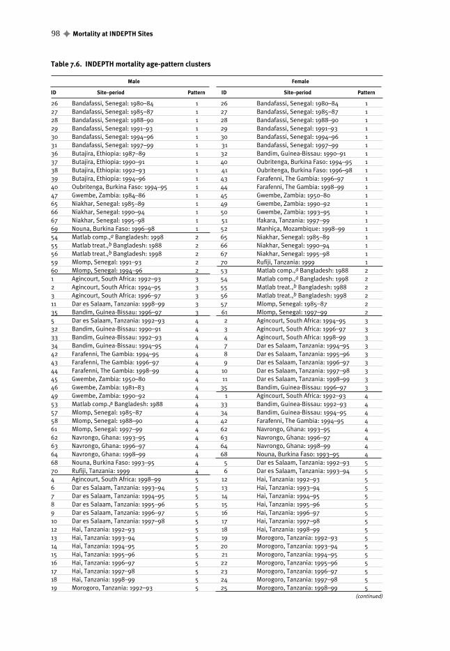
98 ✦ Mortality at INDEPTH Sites
Table 7.6. INDEPTH mortality age-pattern clusters
Male Female
ID Site–period Pattern ID Site–period Pattern
26 Bandafassi, Senegal: 1980–84 1 26 Bandafassi, Senegal: 1980–84 127 Bandafassi, Senegal: 1985–87 1 27 Bandafassi, Senegal: 1985–87 128 Bandafassi, Senegal: 1988–90 1 28 Bandafassi, Senegal: 1988–90 129 Bandafassi, Senegal: 1991–93 1 29 Bandafassi, Senegal: 1991–93 130 Bandafassi, Senegal: 1994–96 1 30 Bandafassi, Senegal: 1994–96 131 Bandafassi, Senegal: 1997–99 1 31 Bandafassi, Senegal: 1997–99 136 Butajira, Ethiopia: 1987–89 1 32 Bandim, Guinea-Bissau: 1990–91 137 Butajira, Ethiopia: 1990–91 1 40 Oubritenga, Burkina Faso: 1994–95 138 Butajira, Ethiopia: 1992–93 1 41 Oubritenga, Burkina Faso: 1996–98 139 Butajira, Ethiopia: 1994–96 1 43 Farafenni, The Gambia: 1996–97 140 Oubritenga, Burkina Faso: 1994–95 1 44 Farafenni, The Gambia: 1998–99 147 Gwembe, Zambia: 1984–86 1 45 Gwembe, Zambia: 1950–80 165 Niakhar, Senegal: 1985–89 1 49 Gwembe, Zambia: 1990–92 166 Niakhar, Senegal: 1990–94 1 50 Gwembe, Zambia: 1993–95 167 Niakhar, Senegal: 1995–98 1 51 Ifakara, Tanzania: 1997–99 169 Nouna, Burkina Faso: 1996–98 1 52 Manhiça, Mozambique: 1998–99 154 Matlab comp.,a Bangladesh: 1998 2 65 Niakhar, Senegal: 1985–89 155 Matlab treat.,b Bangladesh: 1988 2 66 Niakhar, Senegal: 1990–94 156 Matlab treat.,b Bangladesh: 1998 2 67 Niakhar, Senegal: 1995–98 159 Mlomp, Senegal: 1991–93 2 70 Rufiji, Tanzania: 1999 160 Mlomp, Senegal: 1994–96 2 53 Matlab comp.,a Bangladesh: 1988 21 Agincourt, South Africa: 1992–93 3 54 Matlab comp.,a Bangladesh: 1998 22 Agincourt, South Africa: 1994–95 3 55 Matlab treat.,b Bangladesh: 1988 23 Agincourt, South Africa: 1996–97 3 56 Matlab treat.,b Bangladesh: 1998 211 Dar es Salaam, Tanzania: 1998–99 3 57 Mlomp, Senegal: 1985–87 235 Bandim, Guinea-Bissau: 1996–97 3 61 Mlomp, Senegal: 1997–99 25 Dar es Salaam, Tanzania: 1992–93 4 2 Agincourt, South Africa: 1994–95 332 Bandim, Guinea-Bissau: 1990–91 4 3 Agincourt, South Africa: 1996–97 333 Bandim, Guinea-Bissau: 1992–93 4 4 Agincourt, South Africa: 1998–99 334 Bandim, Guinea-Bissau: 1994–95 4 7 Dar es Salaam, Tanzania: 1994–95 342 Farafenni, The Gambia: 1994–95 4 8 Dar es Salaam, Tanzania: 1995–96 343 Farafenni, The Gambia: 1996–97 4 9 Dar es Salaam, Tanzania: 1996–97 344 Farafenni, The Gambia: 1998–99 4 10 Dar es Salaam, Tanzania: 1997–98 345 Gwembe, Zambia: 1950–80 4 11 Dar es Salaam, Tanzania: 1998–99 346 Gwembe, Zambia: 1981–83 4 35 Bandim, Guinea-Bissau: 1996–97 349 Gwembe, Zambia: 1990–92 4 1 Agincourt, South Africa: 1992–93 453 Matlab comp.,a Bangladesh: 1988 4 33 Bandim, Guinea-Bissau: 1992–93 457 Mlomp, Senegal: 1985–87 4 34 Bandim, Guinea-Bissau: 1994–95 458 Mlomp, Senegal: 1988–90 4 42 Farafenni, The Gambia: 1994–95 461 Mlomp, Senegal: 1997–99 4 62 Navrongo, Ghana: 1993–95 462 Navrongo, Ghana: 1993–95 4 63 Navrongo, Ghana: 1996–97 463 Navrongo, Ghana: 1996–97 4 64 Navrongo, Ghana: 1998–99 464 Navrongo, Ghana: 1998–99 4 68 Nouna, Burkina Faso: 1993–95 468 Nouna, Burkina Faso: 1993–95 4 5 Dar es Salaam, Tanzania: 1992–93 570 Rufiji, Tanzania: 1999 4 6 Dar es Salaam, Tanzania: 1993–94 54 Agincourt, South Africa: 1998–99 5 12 Hai, Tanzania: 1992–93 56 Dar es Salaam, Tanzania: 1993–94 5 13 Hai, Tanzania: 1993–94 57 Dar es Salaam, Tanzania: 1994–95 5 14 Hai, Tanzania: 1994–95 58 Dar es Salaam, Tanzania: 1995–96 5 15 Hai, Tanzania: 1995–96 59 Dar es Salaam, Tanzania: 1996–97 5 16 Hai, Tanzania: 1996–97 510 Dar es Salaam, Tanzania: 1997–98 5 17 Hai, Tanzania: 1997–98 512 Hai, Tanzania: 1992–93 5 18 Hai, Tanzania: 1998–99 513 Hai, Tanzania: 1993–94 5 19 Morogoro, Tanzania: 1992–93 514 Hai, Tanzania: 1994–95 5 20 Morogoro, Tanzania: 1993–94 515 Hai, Tanzania: 1995–96 5 21 Morogoro, Tanzania: 1994–95 516 Hai, Tanzania: 1996–97 5 22 Morogoro, Tanzania: 1995–96 517 Hai, Tanzania: 1997–98 5 23 Morogoro, Tanzania: 1996–97 518 Hai, Tanzania: 1998–99 5 24 Morogoro, Tanzania: 1997–98 519 Morogoro, Tanzania: 1992–93 5 25 Morogoro, Tanzania: 1998–99 5
(continued)

Detailed discussions of clustering techniques and this particular algorithm arefound in Kaufman and Rousseeuw (1990), Struyf and Hubert (1997), and MathSoftInc. (1999).8 This routine was applied separately to the male and female data sets,each consisting of four columns (one for each coefficient described above) and70 rows (one for each site–period).
Clusters
The method described above identified five robust clusters in the male data and sevenrobust clusters in the female data, presented in Table 7.6. Because females are subjectto the additional risk of maternal mortality, their age patterns are always more com-plex, and so it is not surprising that two more clusters were identified in the femaledata. Categorizing the male data into the seven female clusters produces seven maleclusters that can be directly compared with the female clusters.
In many cases, periods from the same site are grouped in the same cluster,reassuring us that the clustering algorithm is identifying and grouping fundamentallysimilar mortality schedules. Where periods from the same site are assigned to variousclusters, mortality has been changing significantly over time, and the mortality sched-ules from two periods are substantially different.
Mortality patterns
After the clusters are identified, a characteristic age pattern of mortality is identifiedfor each cluster. In keeping with the use of the component model of mortality, wethen calculate, for each of the 15 coefficients derived from the regression of the indi-vidual site–period mortality schedules on the 15 components of INDEPTH mortality,the weighted average across the site–periods in each cluster. The weights used are theperson–years of observation in each site–period. This yields the average amount of
INDEPTH Mortality Patterns for Africa ✦ 99
Table 7.6. (concluded)
Male Female
ID Site–period Pattern ID Site–period Pattern
20 Morogoro, Tanzania: 1993–945 5 36 Butajira, Ethiopia: 1987–89 621 Morogoro, Tanzania: 1994–95 5 37 Butajira, Ethiopia: 1990–91 622 Morogoro, Tanzania: 1995–96 5 38 Butajira, Ethiopia: 1992–93 623 Morogoro, Tanzania: 1996–97 5 39 Butajira, Ethiopia: 1994–96 624 Morogoro, Tanzania: 1997–98 5 58 Mlomp, Senegal: 1988–90 625 Morogoro, Tanzania: 1998–99 5 69 Nouna, Burkina Faso: 1996–98 641 Oubritenga, Burkina Faso: 1996–98 5 46 Gwembe, Zambia: 1981–83 748 Gwembe, Zambia: 1987–89 5 47 Gwembe, Zambia: 1984–86 750 Gwembe, Zambia: 1993–95 5 48 Gwembe, Zambia: 1987–89 751 Ifakara, Tanzania: 1997–995 5 59 Mlomp, Senegal: 1991–93 752 Manhiça, Mozambique: 1998–99 5 60 Mlomp, Senegal: 1994–96 7
a Comparison area.b Treatment area.
8 A number of clustering techniques were applied to both the raw and the transformed data and to the coefficient vectors, includingagglomerative hierarchical clustering, partitioning around K-means, partitioning around K-medoids, fuzzy partitioning, and divisivehierarchical clustering. Three different statistical software packages — STATA (StataCorp 1997), S-PLUS (MathSoft Inc. 1999), andMVSP (Multi-Variate Statistical Package [KCS 1998]) — were used, and in each case all of their clustering routines were tried. All ofthe methods produced essentially the same clusters but differed in the clarity of their output and in how they managed ambiguouscases. The agglomerative hierarchical algorithm provided with S-PLUS was eventually chosen, based on its clear and robust theoreticalunderpinnings and the fact that its output is easily understood and interpreted. Moreover, it appeared to provide the most robust clus-ters and the most efficient means of categorizing ambiguous cases.
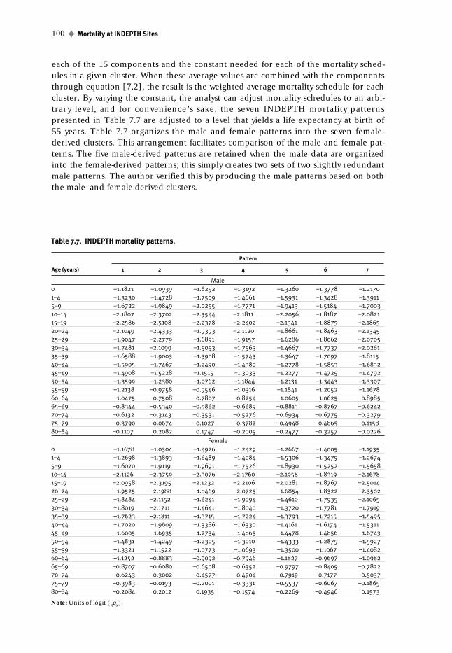
each of the 15 components and the constant needed for each of the mortality sched-ules in a given cluster. When these average values are combined with the componentsthrough equation [7.2], the result is the weighted average mortality schedule for eachcluster. By varying the constant, the analyst can adjust mortality schedules to an arbi-trary level, and for convenience’s sake, the seven INDEPTH mortality patternspresented in Table 7.7 are adjusted to a level that yields a life expectancy at birth of55 years. Table 7.7 organizes the male and female patterns into the seven female-derived clusters. This arrangement facilitates comparison of the male and female pat-terns. The five male-derived patterns are retained when the male data are organizedinto the female-derived patterns; this simply creates two sets of two slightly redundantmale patterns. The author verified this by producing the male patterns based on boththe male- and female-derived clusters.
100 ✦ Mortality at INDEPTH Sites
Table 7.7. INDEPTH mortality patterns.
Pattern
Age (years) 1 2 3 4 5 6 7
Male0 –1.1821 –1.0939 –1.6252 –1.3192 –1.3260 –1.3778 –1.21701–4 –1.3230 –1.4728 –1.7509 –1.4661 –1.5931 –1.3428 –1.39115–9 –1.6722 –1.9849 –2.0255 –1.7771 –1.9413 –1.5184 –1.700310–14 –2.1807 –2.3702 –2.3544 –2.1811 –2.2056 –1.8187 –2.082115–19 –2.2586 –2.5108 –2.2378 –2.2402 –2.1341 –1.8875 –2.186520–24 –2.1049 –2.4333 –1.9393 –2.1120 –1.8661 –1.8463 –2.134525–29 –1.9047 –2.2779 –1.6891 –1.9157 –1.6286 –1.8062 –2.070530–34 –1.7481 –2.1099 –1.5053 –1.7563 –1.4667 –1.7737 –2.026135–39 –1.6588 –1.9003 –1.3908 –1.5743 –1.3647 –1.7097 –1.811540–44 –1.5905 –1.7467 –1.2490 –1.4380 –1.2778 –1.5853 –1.683245–49 –1.4908 –1.5228 –1.1515 –1.3033 –1.2277 –1.4725 –1.479250–54 –1.3599 –1.2380 –1.0762 –1.1844 –1.2131 –1.3443 –1.330755–59 –1.2138 –0.9758 –0.9546 –1.0316 –1.1841 –1.2052 –1.167860–64 –1.0475 –0.7508 –0.7807 –0.8254 –1.0605 –1.0625 –0.898565–69 –0.8344 –0.5340 –0.5862 –0.6689 –0.8813 –0.8767 –0.624270–74 –0.6132 –0.3143 –0.3531 –0.5276 –0.6934 –0.6775 –0.327975–79 –0.3790 –0.0674 –0.1027 –0.3782 –0.4948 –0.4865 –0.115880–84 –0.1107 0.2082 0.1747 –0.2005 –0.2477 –0.3257 –0.0226
Female0 –1.1678 –1.0304 –1.4926 –1.2429 –1.2667 –1.4005 –1.19351–4 –1.2698 –1.3893 –1.6489 –1.4084 –1.5306 –1.3479 –1.26745–9 –1.6070 –1.9119 –1.9691 –1.7526 –1.8930 –1.5252 –1.565810–14 –2.1126 –2.3759 –2.3076 –2.1760 –2.1958 –1.8319 –2.167815–19 –2.0958 –2.3195 –2.1232 –2.2106 –2.0281 –1.8767 –2.501420–24 –1.9525 –2.1988 –1.8469 –2.0725 –1.6854 –1.8322 –2.350225–29 –1.8484 –2.1152 –1.6241 –1.9094 –1.4610 –1.7935 –2.106530–34 –1.8019 –2.1711 –1.4641 –1.8040 –1.3720 –1.7781 –1.791935–39 –1.7623 –2.1811 –1.3715 –1.7224 –1.3793 –1.7215 –1.549540–44 –1.7020 –1.9609 –1.3386 –1.6330 –1.4161 –1.6174 –1.531145–49 –1.6005 –1.6935 –1.2734 –1.4865 –1.4478 –1.4856 –1.674350–54 –1.4831 –1.4249 –1.2305 –1.3010 –1.4333 –1.2875 –1.592755–59 –1.3321 –1.1522 –1.0773 –1.0693 –1.3500 –1.1067 –1.408260–64 –1.1252 –0.8883 –0.9092 –0.7946 –1.1827 –0.9697 –1.098265–69 –0.8707 –0.6080 –0.6508 –0.6352 –0.9797 –0.8405 –0.782270–74 –0.6243 –0.3002 –0.4577 –0.4904 –0.7919 –0.7177 –0.503775–79 –0.3983 –0.0193 –0.2001 –0.3331 –0.5537 –0.6067 –0.186580–84 –0.2084 0.2012 0.1935 –0.1574 –0.2269 –0.4946 0.1573
Note: Units of logit (nqx).

Figures 7.7 and 7.8 plot the seven INDEPTH age patterns of mortality for malesand females, respectively. Figures 7.9–7.15 compare each of the seven INDEPTH agepatterns of mortality for males and females. The patterns are arbitrarily named 1–7,9
and a discussion of the patterns accompanies the plots.
Figure 7.7. Seven INDEPTH age patterns of mortality for males, adjusted to yield a life expectancy at birth of 55 years.
Figure 7.8. Seven INDEPTH age patterns of mortality for females, adjusted to yield a life expectancy at birth of 55 years.
1-4 5-910
-1415
-1920-2
4
40-44
30-34
25-29
35-39
45-49
50-54
55-59
60-64
80-84
70-74
65-69
75-79
Lo
git
of
the
pro
ba
bil
ity
of
dy
ing
: lo
git
(n
qx)
Age group (years)
0.50
0.25
0.00
-0.25
-0.50
-0.75
-1.00
-1.25
-1.50
-1.75
-2.00
-2.25
-2.50
-2.75
-3.00
0
xxxx
x
x
x
xxxx
xx
xxxx xxxxxxxxxxxxxxxxxxxxxxxxxxxxxxxx
xx
xxxxxxxx
xx
x
xx
1 3 5xx 7 4 62
1-4 5-910
-1415
-1920-2
4
40-44
30-34
25-29
35-39
45-49
50-54
55-59
60-64
80-84
70-74
65-69
75-79
0.50
0.25
0.00
-0.25
-0.50
-0.75
-1.00
-1.25
-1.50
-1.75
-2.00
-2.25
-2.50
-2.75
-3.00
Lo
git
of
the
pro
ba
bil
ity
of
dy
ing
: lo
git
(n
qx)
0
1 3 5xx 7 4 6
xxx
xxxxx
xxxxxxxx
xxxxxxxxxxxxxxxxxxxxxxxxxxxxx
xxx
xxx
xxxxxxx
xxxxx
xxx
xxx
x
x
2
22
INDEPTH Mortality Patterns for Africa ✦ 101
9 This is done to avoid the potential stigmatization from use of more descriptive names.

Figure 7.9. INDEPTH mortality pattern 1, adjusted to yield a life expectancy at birth of 55 years.
Pattern 1
The first pattern (Figure 7.9) is similar to the CD North and UN Latin Americanmodel life-table age patterns of mortality (see “Comparisons with the Coale andDemeny and United Nations model life tables,” below). There is no indication thatHIV–AIDS affects pattern 1, and the male and female age patterns are similar, withthe exception of a bulge in the female pattern during the reproductive years, presum-ably caused by maternal mortality. Pattern 1 is primarily derived from sites in WestAfrica over the entire period covered by the INDEPTH data set. HIV–AIDS has not yetbecome as significant a problem in West Africa as it is in Central and southern Africa,so a large impact of AIDS is not expected to be seen in the data from West Africa. It isworth noting that child mortality between the ages of 1 and 9 is significant and sub-stantially elevated above that shown by the most similar existing models, below. This isin keeping with the fact that malaria is a significant cause of death in West Africa, andit has a large impact on those age groups.
1-4 5-910
-1415
-1920-2
4
40-44
30-34
25-29
35-39
45-49
50-54
55-59
60-64
80-84
70-74
65-69
75-79
Age group (years)
0.50
0.25
0.00
-0.25
-0.50
-0.75
-1.00
-1.25
-1.50
-1.75
-2.00
-2.25
-2.50
-2.75
-3.00
0
Male Female
Lo
git
of
the
pro
ba
bil
ity
of
dy
ing
: lo
git
(n
qx)
102 ✦ Mortality at INDEPTH Sites

Figure 7.10. INDEPTH mortality pattern 2, adjusted to yield a life expectancy at birth of 55 years.
Pattern 2
Pattern 2 (Figure 7.10) is the only pattern to contain significant contributions fromAsia, and it is in fact dominated by data from the Matlab project, in Bangladesh. Theonly other site to contribute data to this pattern is the Mlomp site, in Senegal. Again,the male and female patterns are similar, with the exception of maternal mortality.However, pattern 2 is strikingly different from all of the others in that the mortality ofchildren, teenagers, and young adults is comparatively very low, and correspondinglythe mortality of older adults is comparatively high. In keeping with the fact that thedata contributing to this pattern come from Bangladesh and Senegal, it is not surpris-ing that there is no evidence at all of an HIV–AIDS impact. Pattern 2 is very similar tothe UN South Asia pattern, as it should be, coming largely from South Asia (seebelow).
1-4 5-910
-1415
-1920-2
4
40-44
30-34
25-29
35-39
45-49
50-54
55-59
60-64
80-84
70-74
65-69
75-79
Lo
git
of
the
pro
ba
bil
ity
of
dy
ing
: lo
git
(n
qx)
Age group (years)
0.50
0,25
0.00
-0.25
-0.50
-0.75
-1.00
-1.25
-1.50
-1.75
-2.00
-2.25
-2.50
-2.75
-3.00
0
Male Female
INDEPTH Mortality Patterns for Africa ✦ 103
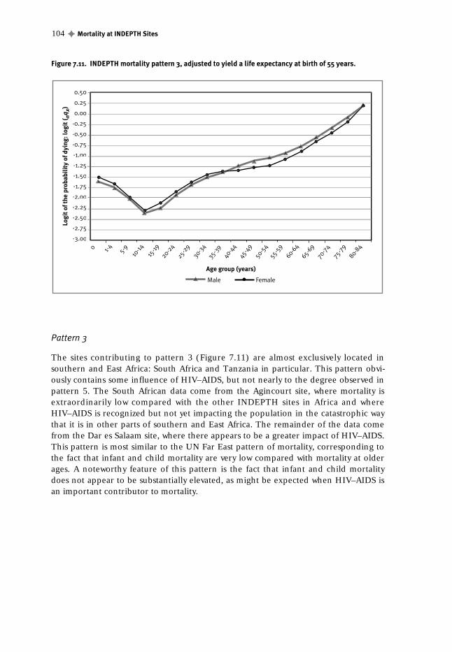
Figure 7.11. INDEPTH mortality pattern 3, adjusted to yield a life expectancy at birth of 55 years.
Pattern 3
The sites contributing to pattern 3 (Figure 7.11) are almost exclusively located insouthern and East Africa: South Africa and Tanzania in particular. This pattern obvi-ously contains some influence of HIV–AIDS, but not nearly to the degree observed inpattern 5. The South African data come from the Agincourt site, where mortality isextraordinarily low compared with the other INDEPTH sites in Africa and whereHIV–AIDS is recognized but not yet impacting the population in the catastrophic waythat it is in other parts of southern and East Africa. The remainder of the data comefrom the Dar es Salaam site, where there appears to be a greater impact of HIV–AIDS.This pattern is most similar to the UN Far East pattern of mortality, corresponding tothe fact that infant and child mortality are very low compared with mortality at olderages. A noteworthy feature of this pattern is the fact that infant and child mortalitydoes not appear to be substantially elevated, as might be expected when HIV–AIDS isan important contributor to mortality.
1-4 5-910
-1415
-1920-2
4
40-44
30-34
25-29
35-39
45-49
50-54
55-59
60-64
80-84
70-74
65-69
75-79
Lo
git
of
the
pro
ba
bil
ity
of
dy
ing
: lo
git
(n
qx)
Age group (years)
0.50
0.25
0.00
-0.25
-0.50
-0.75
-1.00
-1.25
-1.50
-1.75
-2.00
-2.25
-2.50
-2.75
-3.00
0
Male Female
104 ✦ Mortality at INDEPTH Sites

Figure 7.12. INDEPTH mortality pattern 4, adjusted to yield a life expectancy at birth of 55 years.
Pattern 4
Pattern 4 (Figure 7.12) is a variation on pattern 1, with the important difference mani-fested in the 35-69 years age range. At all other ages, patterns 1 and 4 are negligiblydifferent, except that infant and child mortality in pattern 4 is consistently slightlylower than in pattern 1. But between ages 35 and roughly 69 years, pattern 4 revealssignificantly higher mortality than pattern 1. This pattern is most similar to the UNGeneral pattern for females and UN Latin America for males. As was the case with pat-tern 1, most of the data contributing to pattern 4 come from West Africa.
1-4 5-910
-1415
-1920-2
4
40-44
30-34
25-29
35-39
45-49
50-54
55-59
60-64
80-84
70-74
65-69
75-79
Lo
git
of
the
pro
ba
bil
ity
of
dy
ing
: lo
git
(n
qx)
Age group (years)
0.50
0.25
0.00
-0.25
-0.50
-0.75
-1.00
-1.25
-1.50
-1.75
-2.00
-2.25
-2.50
-2.75
-3.00
0
Male Female
INDEPTH Mortality Patterns for Africa ✦ 105

Figure 7.13. INDEPTH mortality pattern 5, adjusted to yield a life expectancy at birth of 55 years.
Pattern 5
The HIV–AIDS pattern of mortality is most clearly visible in pattern 5 (Figure 7.13).The data contributing to pattern 5 are derived from the three Tanzanian sites run bythe Adult Morbidity and Mortality Project in Dar es Salaam, Hai, and Morogoro. Avery striking bulge appears in the mortality of males between the ages of 20 and 54years and for females between the ages of 15 and 49 years. Additionally, the femalebulge is significantly narrower and more pronounced, corresponding to the fact thatthe female population is infected earlier and within a tighter age range. This pattern isnot particularly similar to any of the existing model patterns, but it is most closelymatched with the UN General (female) and UN Latin American (male) model pat-terns. Pattern 5 differs from pattern 3 mainly in the shape of the HIV–AIDS impact.The effect is more diffuse with age in pattern 3, meaning that mortality is elevatedthrough a broader age range, the magnitude of the elevation is more consistent, andthe differences between the sexes are less apparent. Pattern 3 is derived largely fromthe Dar es Salaam data, and this may reflect the fact that the epidemic is more maturein Dar es Salaam and has consequently had enough time to infect a wider age range ofpeople of both sexes. As with pattern 3, it is worth noting that infant and child mortal-ity do not appear to be substantially affected in a manner comparable to adult mortal-ity, and this is in contradiction to what is known about HIV prevalence and verticaltransmission. Further investigation is needed to determine why this effect is notprominently measured in these data.
1-4 5-910
-1415
-1920-2
4
40-44
30-34
25-29
35-39
45-49
50-54
55-59
60-64
80-84
70-74
65-69
75-79
Lo
git
of
the
pro
ba
bil
ity
of
dy
ing
: lo
git
(n
qx)
Age group (years)
0.50
0.25
0.00
-0.25
-0.50
-0.75
-1.00
-1.25
-1.50
-1.75
-2.00
-2.25
-2.50
-2.75
-3.00
0
Male Female
106 ✦ Mortality at INDEPTH Sites

Figure 7.14. INDEPTH mortality pattern 6, adjusted to yield a life expectancy at birth of 55 years.
Pattern 6
Pattern 6 (Figure 7.14) is one of the two additional patterns identified in the femaledata. It is an interesting pattern that reveals very high mortality of children andteenagers, together with comparatively low mortality of infants and adults of all ages.This pattern is exhibited at sites in northeast and West Africa, with most of the datacoming from Ethiopia. Without additional information, it is impossible to speculateon what may be producing this unique pattern. The male pattern is most similar to theCD North model pattern, and the female pattern is closest to the CD West model,both of which embody high mortality in the same age ranges. They deviate from thosepatterns in that infant mortality is substantially lower than would be found in eithermodel pattern, and child and adolescent mortality is significantly higher: this might becalled the “Super North” pattern.
1-4 5-910
-1415
-1920-2
4
40-44
30-34
25-29
35-39
45-49
50-54
55-59
60-64
80-84
70-74
65-69
75-79
Lo
git
of
the
pro
ba
bil
ity
of
dy
ing
: lo
git
(n
qx)
Age group (years)
0.50
0.25
0.00
-0.25
-0.50
-0.75
-1.00
-1.25
-1.50
-1.75
-2.00
-2.25
-2.50
-2.75
-3.00
0
Male Female
INDEPTH Mortality Patterns for Africa ✦ 107

Figure 7.15. INDEPTH mortality pattern 7, adjusted to yield a life expectancy at birth of 55 years.
Pattern 7
Pattern 7 (Figure 7.15), the other additional pattern identified in the female data, isalso of interest. It is derived from two sites in Central and West Africa. The reason whyit was identified in the female data is obvious: a very substantial bulge appears in thefemale age pattern between ages 25 and 44 years. This most likely results from veryserious maternal mortality, the risk of which increases with age. The site in Zambia is arural site without easy access to modern medical facilities, and this may contribute toan unusual risk of maternal mortality. The corresponding male pattern is similar topattern 6, and both are similar to the CD North model pattern. The CD North modelpattern contains higher child and teenage mortality, coupled with comparatively lowmortality at older ages. This is consistent with the fact that malaria is an importantcontributor to mortality at both sites.
Comparisons with the Coale and Demeny and
United Nations model life tables
The INDEPTH mortality patterns are explicitly compared with the existing CD and UNmodels to ensure that they are indeed new patterns and to demonstrate exactly howthey differ from the existing model mortality patterns. The method used is a simpleminimum sum of squared differences. Each INDEPTH mortality pattern is comparedwith all of the existing CD and UN model mortality patterns: CD patterns North,South, East, and West; and UN patterns Latin America, Chile, South Asia, Far East,and General. For each pair of patterns, the difference between the two is calculated
1-4 5-910
-1415
-1920-2
4
40-44
30-34
25-29
35-39
45-49
50-54
55-59
60-64
80-84
70-74
65-69
75-79
Lo
git
of
the
pro
ba
bil
ity
of
dy
ing
: lo
git
(n
qx)
Age group (years)
0.50
0.25
0.00
-0.25
-0.50
-0.75
-1.00
-1.25
-1.50
-1.75
-2.00
-2.25
-2.50
-2.75
-3.00
0
Male Female
108 ✦ Mortality at INDEPTH Sites

for each age group, and those differences are squared and summed to yield the sum(over all ages) of the squared differences (SSD) between the two patterns. For eachINDEPTH pattern, the SDDs derived from the seven comparisons are ranked, and themembers of the pair with the smallest SDD are considered to be most similar. All of themortality patterns used in the comparisons are adjusted to a level corresponding to anlife expectancy at birth of 55 years.10 The SDDs are presented in Table 7.8, where boththe minimum and the next greater SDDs for each comparison are identified.
For each INDEPTH pattern, the age-specific deviations from the closest fitexisting model pattern are calculated and presented in Figures 7.16 and 7.17. Thosefigures clearly reveal that all of the INDEPTH patterns are systematically differentfrom the existing model mortality patterns. Both figures reveal clear peaks in the devi-ations for children (1-14 years) and young to middle-aged adults (25-49 years).Interestingly, infant and child mortality between the ages of 1 and 4 years is generallylower than the corresponding pattern. The peak in the deviations during childhoodmay be due to malaria and other diseases that have a large impact on children inAfrica but not elsewhere in the world, and it is clear that continued investigation isneeded to identify all of the factors contributing to childhood deviations. The peakduring the adult years is most pronounced for patterns 3 and 5, which are the two pat-terns affected by HIV–AIDS, and it is reasonable to assume that this peak is primarilydue to the impact of HIV–AIDS. It is curious to note that infant and child mortality inpatterns 3 and 5 does not appear to be elevated in a manner corresponding to theincrease in adult mortality. This suggests that the HIV–AIDS epidemic does not havean enormous impact on infant and child mortality or that all of the data used to gen-erate patterns 3 and 5 are defective with regard to infants and children. It seemsunlikely that all the data would be defective, along with being defective to the samedegree, and this points to the need for considerable investigation of the impact ofHIV–AIDS on infant and child mortality.
INDEPTH Mortality Patterns for Africa ✦ 109
Table 7.8. Sum of squared differences comparing INDEPTH and existing mortality patterns.
Model
Pattern North South East West LA CH SA FE GL
Male1 0.2670 0.5550 0.7599 0.6035 0.3111 1.1682 0.8744 1.6724 0.64582 1.3819 0.6787 0.6538 0.9190 0.8760 1.0439 0.2265 1.1394 0.69183 1.1060 1.6448 1.2875 0.8313 1.0938 0.9075 2.3094 0.5066 0.7774
4 0.4041 0.7742 0.7219 0.4561 0.3640 0.8273 1.0159 0.9664 0.43445 0.6760 1.4443 1.3789 0.8996 0.7961 1.1767 2.3346 1.6279 1.02656 0.5118 1.4451 1.6459 1.2315 0.9998 2.2118 2.1365 2.5333 1.44867 0.4017 0.4548 0.5344 0.4985 0.4233 1.1231 0.5451 1.1824 0.4866
Female1 0.1763 0.4823 0.4573 0.3666 0.1727 0.6523 0.6724 1.0096 0.34282 1.4695 1.0966 0.8080 1.2731 1.0356 1.0373 0.4703 1.4209 0.97443 1.4447 2.2012 1.5312 1.0859 1.3253 1.1886 2.4018 0.4426 0.9283
4 0.4823 1.0188 0.7003 0.4749 0.3982 0.6471 1.0570 0.6098 0.3752
5 0.7861 1.5676 1.2496 0.7118 0.8045 0.9274 2.1636 0.7916 0.7728
6 0.3860 1.1897 1.2256 0.7723 0.7730 1.4854 1.7386 1.6242 0.93207 0.3837 0.5397 0.4040 0.4859 0.3905 0.7709 0.4704 1.0079 0.4050
Source: CD model (North, South, East, West) is from Coale and Demeny (1966); UN model (Latin America, Chile, South Asia, Far East, General) is from United Nations (1982).Note: CH, Chile; FE, Far East; GL, General; LA, Latin America; SA, South Asia. Bold, minimum; italic, next best.
10 The level of the INDEPTH patterns is set by adjusting the constant term in the component model of morality, and the CD- and UN-model mortality patterns used in the comparisons are generated by the United Nation’s computer program for the analysis of mor-tality data, MortPak-Lite (United Nations 1988), at a level corresponding to a life expectancy at birth of 55 years.

Figure 7.16. Age-specific deviations of INDEPTH male mortality patterns from those of best-fit existingmodels [logit (nqx)], adjusted to yield a life expectancy at birth of 55 years.
Figure 7.17. Age-specific deviations of INDEPTH female mortality patterns from those of best-fit existing models [logit ( nqx)], adjusted to yield a life expectancy at birth of 55 years.
1-4 5-910
-1415
-1920-2
4
40-44
30-34
25-29
35-39
45-49
50-54
55-59
60-64
80-84
70-74
65-69
75-79
De
via
tio
n i
n l
og
it (
nq
x)
valu
es
0.8
0.7
0.6
0.5
0.4
0.3
0.2
0.1
-0.2
-0.3
-0.4
-0.5
-0.6
0
P1–North – P3–Far East x P4–Latin America
xx
xxxxxxx
xx xx x x
xxx
x
x
xxxxx
xx P6–NorthP5–North P7–North
xxx
xx
xxxx
xx xxxx
xx xxx xxxx
xxxx xx
xx
xx
xx
x
x
xxx
xxxx xxxxxxxx
xx
xxxxxx
xxx
xxxxxxxxxx
xxxx
xxx
x
xxx
x
xxxxxx
x
xx
xxxxxxxxxxxx xx
xxx
x
x
xxxx
xxxx
xxxxxxxxx
1-4 5-910
-1415
-1920-2
4
40-44
30-34
25-29
35-39
45-49
50-54
55-59
60-64
80-84
70-74
65-69
75-79
De
via
tio
n i
n l
og
it (
nq
x)
valu
es
0.8
0.7
0.6
0.5
0.4
0.3
0.2
0.1
0.0
-0.1
-0.2
-0.3
-0.4
-0.5
-0.6
0
P1–North P2–South Asia –Far East x P4–Latin America
xx
xx
xxxx
xxx
xxxxxxxxxxxx
xxxxx
xxxx xx xxxx
xxx xxxxxxxx
xxxxxx
xx
xx P6–NorthP5–North P7–North
x
xxx
xxxxxxxx
xx xx
xx
xxxxxx xxxxxxxxxxxx xxxxxxxxxxxxx xxxxx xxxxxxxxxxxxxxxxxxx xxxxxx
xxxxxxxxxxxxxxxxxxxxxxxxxxx
xxxxxxx
xxxxx
110 ✦ Mortality at INDEPTH Sites

Demonstration of the HIV–AIDS model life-table system
Model life-table construction
The component model of mortality is capable of generating (and fitting) a very widerange of arbitrary mortality patterns. This makes it particularly well-suited for the cre-ation of model life tables. To demonstrate how the component model can be used tocreate a set of model life tables, we use the INDEPTH mortality components to isolate(in a set of coefficient deviations) the general age pattern of the impact of HIV–AIDS,and then add that impact in increasing quantities to the INDEPTH pattern-1 mortalityschedule, thus creating a set of life tables with decreasing life expectancies at birth cor-responding to an increasing impact of HIV. The result is a set of life tables with theunderlying age pattern defined by INDEPTH pattern 1 but with various levels ofHIV–AIDS mortality added to that.
Figures 7.18 and 7.19 display the male and female INDEPTH pattern-5 mortal-ity schedules with and without what is presumed to be the increase in mortality due toHIV–AIDS. Figure 7.20 presents the male INDEPTH pattern-1 mortality with and with-out an increase in mortality over the infant and childhood ages.11 In each case, the dif-ference between the two curves is fitted against the first 15 components of mortality(for the appropriate sex) to yield the coefficients presented in Table 7.9.
Figure 7.18. INDEPTH male mortality pattern 5, without and with the presumed increase in mortality due to HIV–AIDS (the HIV–AIDS bulge).
1-4 5-910
-1415
-1920-2
4
40-44
30-34
25-29
35-39
45-49
50-54
55-59
60-64
80-84
70-74
65-69
75-79
Lo
git
of
the
pro
ba
bil
ity
of
dy
ing
: lo
git
(n
qx)
0.50
0.25
0.00
-0.25
-0.50
-0.75
-1.00
-1.25
-1.50
-1.75
-2.00
-2.25
-2.50
-2.75
-3.00
0
Age group (years)
Without HIV–AIDSWith HIV–AIDS
INDEPTH Mortality Patterns for Africa ✦ 111
11 There is no empirical pattern used to create the increase in infant and child mortality. It is simply created so that it could be includedin the model life tables.

Figure 7.19. INDEPTH female mortality pattern 5, without and with the presumed increase in mortalitydue to HIV–AIDS (the HIV–AIDS bulge).
Figure 7.20. INDEPTH male mortality pattern 1, with and without HIV–AIDS mortality for infants and children.
1-4 5-910
-1415
-1920-2
4
40-44
30-34
25-29
35-39
45-49
50-54
55-59
60-64
80-84
70-74
65-69
75-79
Lo
git
of
the
pro
ba
bil
ity
of
dy
ing
: lo
git
(n
qx)
0.50
0.25
0.00
-0.25
-0.50
-0.75
-1.00
-1.25
-1.50
-1.75
-2.00
-2.25
-2.50
-2.75
-3.00
0
Age group (years)
Without HIV–AIDSWith HIV–AIDS
1-4 5-910
-1415
-1920-2
4
40-44
30-34
25-29
35-39
45-49
50-54
55-59
60-64
80-84
70-74
65-69
75-79
Lo
git
of
the
pro
ba
bil
ity
of
dy
ing
: lo
git
(n
qx)
0.50
0.25
0.00
-0.25
-0.50
-0.75
-1.00
-1.25
-1.50
-1.75
-2.00
-2.25
-2.50
-2.75
-3.00
0
Age group (years)
Without HIV–AIDSWith HIV–AIDS
112 ✦ Mortality at INDEPTH Sites

The model life tables are constructed to produce a family of life tables with theunderlying mortality of INDEPTH pattern-1 mortality. The HIV–AIDS pattern of mor-tality is added to each of the members of the family in amounts sufficient to reducethe life expectancy at birth in 5-year increments. Equation [7.5] is a simple extensionof the component model of mortality that describes the relationship used to accom-plish this. In this case, the (n + 1) � 1 vector d� of HIV–AIDS coefficient deviations ismultiplied by � and added to the (n + 1) � 1 vector of coefficients, a�.12 The scalingfactor � determines how much of the HIV–AIDS pattern to add to the basic pattern ofmortality represented by the vector of coefficients, a�. Once that addition has beenaccomplished, the resulting vector is premultiplied by the matrix of components C �
to yield the logit-transformed probabilities of dying, logit (nq x). The relationship gov-erning the HIV-augmented model life table is given by the following equation:
m = C�(a� + �d�) [7.5]
where m , C�, a� , �, and d� are as defined above. Expanding this around the row forthe 20–24 age group reveals
. . . .. . . .. . . .
logit(5q20) = 5C20. (ai + � . di) + ... + 5C20
. (an + � . dn ) + 1.(ac + � . dc ). . . .. . . .. . . .
INDEPTH Mortality Patterns for Africa ✦ 113
Table 7.9. Coefficient values estimated in fit of HIV-derived
deviations in logit (nqx) on the mortality
components.
Fit of adult deviations Fit of child deviations
Component Male Female Male Female
1 0.001 794 –0.004 217 –0.002 822 –0.003 9262 0.069 515 0.086 812 0.030 939 0.024 0633 –0.087 825 –0.093 468 0.048 722 0.046 5464 –0.046 538 0.007 340 –0.030 034 –0.033 0625 0.014 998 –0.053 602 –0.002 600 0.017 2916 0.007 024 0.071 480 –0.042 015 0.044 1767 0.057 843 –0.026 918 –0.001 601 0.029 7698 0.067 342 0.011 817 0.015 266 –0.036 0319 –0.035 387 0.055 790 –0.012 263 0.029 19910 –0.030 752 0.070 519 0.028 062 0.006 90311 –0.048 241 0.037 762 –0.013 452 0.043 73612 0.040 329 –0.028 917 –0.001 339 –0.004 03113 0.003 209 0.082 885 0.032 003 0.025 62114 0.091 293 0.089 362 0.050 373 –0.013 28715 0.126 678 –0.048 030 –0.008 452 0.030 330
Constant 0.062 364 0.079 854 –0.030 420 –0.028 344
12 Remember that the prime (�) indicates that the matrices and vectors include the column and row needed to store the constant and itscoefficient. Also, n is the number of components used, and g is the number of age groups.
ni

where 5C20 is the value of the i th component for the 20–24 age group; a i is the valueof the coefficient on the i th component; � is a single scalar applied to the vector ofcoefficient deviations; d i is the coefficient deviation for the i th component; a c is theconstant term, which takes the same value for all age groups; and d c is the deviationfor the constant term. Each of the column vectors contains g elements, one for eachage group.
Once the logit (nq x) values have been calculated, the inverse logit produces val-ues for nq x to be substituted into a life table and used to calculate its other columns,including life expectancy. The model life tables are calculated through an iterative,target-seeking process that varies � until the desired value for the life expectancy isattained (see Figures 7A.1–7A6 and Tables 7A.1–7A.4 in the Annex).
Conclusion
Data describing mortality at 19 sites in Africa and Asia are used to identify seven newage patterns of mortality, six of which originate solely from Africa. A componentmodel of mortality is constructed from the raw data and used to identify clusters ofsimilar age patterns of mortality, and these patterns are compared with the existingCD and UN model life-table age patterns of mortality and demonstrated to be system-atically and individually different from the existing models. This finding supports thenotion that unique age patterns of mortality occur in Africa and that routine demo-graphic and epidemiological estimations calculated from African data must take thisinto account. To make these data useful to practicing demographers and epidemiolo-gists, a set of model life tables based on these patterns must be constructed. INDEPTHis pursuing the construction of a set of INDEPTH model life tables for Africa, usingthe component model of mortality and based on the age patterns of mortality pre-sented here.
114 ✦ Mortality at INDEPTH Sites
i

ANNEX: AIDS-DECREMENTED MODEL LIFE TABLES
Figure 7A.1. Male life-table probability of dying (nqx), decreased by AIDS mortality in 5-year increments(initial life expectancy at birth, 45 years).
Figure 7A.2. Female life-table probability of dying (nqx), decreased by AIDS mortality in 5-year increments (initial life expectancy at birth, 45 years).
1-4 5-9
20-24
40-44
30-34
25-29
35-39
45-49
50-54
55-59
60-64
80-84
70-74
65-69
75-79
Lif
e-t
ab
le p
rob
ab
ilit
y o
f d
yin
g,
nq
x
Age group (years)
0.700.650.600.550.500.450.400.350.300.250.200.150.100.050.00
0
e0 = 45 xxe0 = 40 e0 = 35 e0 = 30 e0 = 25
xxxxxxxxxxxxxx
xxxxxxxxxxxxxx xxxxxx
xx
xxx
xx
xxx
xxx
xxxxxxxxxxxxxxxxx xxxxxxxxxxxx
xxxxxxxxxxx
xxx
xxxxxx
xxxx
xx
xxxxxx
1-4 5-9
40-44
30-34
25-29
35-39
45-49
50-54
55-59
60-64
80-84
70-74
65-69
75-79
Lif
e-t
ab
le p
rob
ab
ilit
y o
f d
yin
g,
nq
x
Age group (years)
0.700.650.600.550.500.450.400.350.300.250.200.150.100.050.00
0
e0 = 45 xxe0 = 40 e0 = 35 e0 = 30 e0 = 25
xxxxxxxx
xxxxxxxx
xxxxxxxxxxx
xxxxxx
xxxxxxxx
x
x
xxx
x
xx
xxxxxxxxxxxxxxxxxxx
xxxxxxxxxx
xx
xx
xxxxx
xxxxxxxx
xxxxxxxxx
xx
xx
xxxxx
INDEPTH Mortality Patterns for Africa ✦ 115

Figure 7A.3. Male life-table probability of surviving (Px), decreased by AIDS mortality in 5-yearincrements (initial life expectancy at birth, 45 years).
Figure 7A.4. Female life-table probability of surviving (Px), decreased by AIDS mortality in 5-yearincrements (initial life expectancy at birth, 45 years).
1-4 5-910
-1415
-1920-2
4
40-44
30-34
25-29
35-39
45-49
50-54
55-59
60-64
80-84
70-74
65-69
75-79
Lif
e-t
ab
le p
rob
ab
ilit
y o
f s
urv
ivin
g, P
x
Age group (years)
1.0
0.9
0.8
0.7
0.6
0.5
0.4
0.3
0.2
0.1
0.0
0
e0 = 45 xxe0 = 40 e0 = 35 e0 = 30 e0 = 25
xxxxxxxxxxxxxxxxxx
xxx
xx
xx
xxxxxxxxxxxxx
xx
xxxxxxxxx
1-4 5-910
-1415
-1920-2
4
40-44
30-34
25-29
35-39
45-49
50-54
55-59
60-64
80-84
Lif
e-t
ab
le p
rob
ab
ilit
y o
f s
urv
ivin
g, P
x
Age group (years)
1.0
0.9
0.8
0.7
0.6
0.5
0.4
0.3
0.2
0.1
0.0
0
e0 = 45 xxe0 = 40 e0 = 35 e0 = 30 e0 = 25
xxxxx
xxx
xxxx xx xx
xxxx
xxx
xxxxxxxxxxxx
xx
xx xx xx xx xxxx
xxx
xx xxx
xxxxx
116 ✦ Mortality at INDEPTH Sites

Figure 7A.5. Male life expectancy (ex, or average remaining lifetime for a person who survives to the beginning of the indicated age interval), decreased by AIDS mortality in 5-year increments (initial life expectancy at birth, 45 years).
Figure 7A.6. Female life expectancy (ex, or average remaining lifetime for a person who survives to the beginning of the indicated age interval), decreased by AIDS mortality in 5-yearincrements (initial life expectancy at birth, 45 years).
1-4 5-910
-1415
-1920-2
4
40-44
30-34
25-29
35-39
45-49
50-54
55-59
60-64
80-84
70-74
65-69
75-79
Lif
e e
xp
ect
an
cy,
ex (
ye
ars
)
Age group (years)
65
60
55
50
45
40
35
30
25
20
15
10
5
0
0
e0 = 45 xxe0 = 40 e0 = 35 e0 = 30 e0 = 25
xxxxxxxxxxxxxxxx
xxxxxxxxxxxxxxxxxxxxxxxxxxxx
xxxxxxxxxxxxxxxxxxxxxxx
xxxxxxxxxxxxxxxxx
xxxxxxxx
xxxxx
xxxxxxx
xxxxxxxx
1-4 5-910
-1415
-1920-2
4
40-44
30-34
25-29
35-39
45-49
50-54
55-59
60-64
80-84
70-74
65-69
75-79
Lif
e e
xp
ect
an
cy,
ex (
ye
ars
)
Age group (years)
65
60
55
50
45
40
35
30
25
20
15
10
5
0
0
e0 = 45 xxe0 = 40 e0 = 35 e0 = 30 e0 = 25
xxxxxxxxxxxxx
xxxxxxxxxxxxxxxxxxxxxxxxxxxxxxxxxxxxxx
xxxxxxxxxxx
xxxx
xxxx
xxxxxxxxx
xxxxxxx
INDEPTH Mortality Patterns for Africa ✦ 117

118 ✦ Mortality at INDEPTH Sites
Ta
ble
7A
.1.
Mo
de
l li
fe t
ab
les
fo
r IN
DE
PT
H p
att
ern
1:
life
ex
pe
cta
ncy
of
60
.0 y
ea
rs d
ecr
em
en
ted
by
HIV
–A
IDS
mo
rta
lity
.
Re
du
ctio
n i
n e
0(y
ea
rs)
Ma
leF
em
ale
Ag
e (
ye
ars
)0
.05
.010
.015
.02
0.0
0.0
5.0
10.0
15.0
20
.0
nq
x
00.
068
354
0.07
6 01
30.
081
963
0.08
7 23
00.
092
413
0.07
0 64
80.
076
841
0.08
1 02
50.
084
427
0.08
7 54
6
1–4
0.05
1 41
40.
055
626
0.05
8 83
50.
061
634
0.06
4 35
50.
057
153
0.06
1 25
00.
063
991
0.06
6 20
40.
068
222
5–9
0.02
6 08
50.
027
408
0.02
8 39
40.
029
240
0.03
0 05
10.
030
118
0.03
1 52
30.
032
448
0.03
3 18
70.
033
854
10–1
40.
010
159
0.01
0 16
20.
010
164
0.01
0 16
50.
010
167
0.01
1 86
20.
011
849
0.01
1 84
00.
011
834
0.01
1 82
8
15–1
90.
008
511
0.00
9 05
70.
009
469
0.00
9 82
50.
010
169
0.01
1 45
20.
012
871
0.01
3 86
10.
014
683
0.01
5 45
0
20–2
40.
011
362
0.01
5 59
10.
019
531
0.02
3 53
70.
027
986
0.01
5 35
90.
027
156
0.03
8 81
80.
051
094
0.06
4 94
4
25–2
90.
016
697
0.03
0 94
90.
047
772
0.06
8 06
10.
093
905
0.01
8 94
70.
048
985
0.08
7 58
90.
134
870
0.19
3 18
5
30–3
40.
022
747
0.04
9 92
00.
085
953
0.13
2 37
20.
193
248
0.02
1 03
80.
059
561
0.11
1 71
00.
176
657
0.25
6 09
6
35–3
90.
027
520
0.06
1 02
00.
105
336
0.16
1 76
20.
234
230
0.02
2 69
40.
054
981
0.09
4 38
00.
140
965
0.19
6 94
3
40–4
40.
031
406
0.06
8 63
10.
117
010
0.17
7 53
80.
253
830
0.02
5 47
20.
045
196
0.06
4 55
20.
084
710
0.10
7 14
9
45–4
90.
038
409
0.06
9 16
00.
103
772
0.14
3 42
80.
191
043
0.03
0 37
10.
038
020
0.04
3 80
20.
048
876
0.05
3 82
9
50–5
40.
048
610
0.06
4 73
70.
079
184
0.09
3 38
10.
108
628
0.03
8 94
60.
041
139
0.04
2 59
20.
043
757
0.04
4 81
3
55–5
90.
063
546
0.06
8 23
00.
071
772
0.07
4 84
60.
077
819
0.05
1 95
80.
051
479
0.05
1 17
80.
050
944
0.05
0 73
8
60–6
40.
087
337
0.08
7 15
60.
087
026
0.08
6 91
90.
086
818
0.07
6 85
90.
076
105
0.07
5 63
00.
075
262
0.07
4 93
7
65–6
90.
129
704
0.13
0 24
90.
130
641
0.13
0 96
70.
131
271
0.12
1 95
10.
120
671
0.11
9 86
50.
119
240
0.11
8 69
0
70–7
40.
186
536
0.18
5 70
70.
185
117
0.18
4 62
60.
184
170
0.18
0 79
20.
175
174
0.17
1 68
10.
168
998
0.16
6 65
3
75–7
90.
265
402
0.26
2 57
40.
260
564
0.25
8 90
00.
257
356
0.25
4 47
30.
251
341
0.24
9 36
80.
247
837
0.24
6 48
9
80–8
40.
384
085
0.38
5 58
50.
386
658
0.38
7 55
10.
388
385
0.34
3 50
90.
361
047
0.37
2 37
60.
381
299
0.38
9 26
3
Px
01.
000
000
1.00
0 00
01.
000
000
1.00
0 00
01.
000
000
1.00
0 00
01.
000
000
1.00
0 00
01.
000
000
1.00
0 00
0
1–4
0.93
1 64
60.
923
987
0.91
8 03
70.
912
770
0.90
7 58
70.
929
352
0.92
3 15
90.
918
975
0.91
5 57
30.
912
454
5–9
0.88
3 74
70.
872
589
0.86
4 02
40.
856
513
0.84
9 18
00.
876
236
0.86
6 61
60.
860
169
0.85
4 95
80.
850
205
10–1
40.
860
695
0.84
8 67
30.
839
491
0.83
1 46
80.
823
661
0.84
9 84
60.
839
297
0.83
2 25
80.
826
585
0.82
1 42
2
15–1
90.
851
951
0.84
0 04
90.
830
959
0.82
3 01
60.
815
287
0.83
9 76
50.
829
352
0.82
2 40
30.
816
803
0.81
1 70
7
20–2
40.
844
700
0.83
2 44
10.
823
091
0.81
4 93
00.
806
996
0.83
0 14
80.
818
677
0.81
1 00
40.
804
810
0.79
9 16
6
25–2
90.
835
103
0.81
9 46
20.
807
015
0.79
5 74
90.
784
412
0.81
7 39
70.
796
445
0.77
9 52
30.
763
690
0.74
7 26
5
30–3
40.
821
160
0.79
4 10
00.
768
462
0.74
1 59
00.
710
751
0.80
1 91
00.
757
431
0.71
1 24
60.
660
691
0.60
2 90
5
35–3
90.
802
481
0.75
4 45
90.
702
410
0.64
3 42
40.
573
400
0.78
5 03
90.
712
318
0.63
1 79
30.
543
975
0.44
8 50
3
40–4
40.
780
396
0.70
8 42
10.
628
421
0.53
9 34
20.
439
092
0.76
7 22
30.
673
154
0.57
2 16
40.
467
294
0.36
0 17
3
45–4
90.
755
887
0.65
9 80
20.
554
890
0.44
3 58
90.
327
637
0.74
7 68
10.
642
730
0.53
5 23
00.
427
709
0.32
1 58
1
50–5
40.
726
854
0.61
4 17
00.
497
308
0.37
9 96
60.
265
045
0.72
4 97
30.
618
293
0.51
1 78
60.
406
804
0.30
4 27
1
55–5
90.
691
522
0.57
4 41
10.
457
929
0.34
4 48
40.
236
253
0.69
6 73
90.
592
857
0.48
9 98
80.
389
004
0.29
0 63
6

INDEPTH Mortality Patterns for Africa ✦ 119
60–6
40.
647
578
0.53
5 21
80.
425
062
0.31
8 70
10.
217
868
0.66
0 53
70.
562
337
0.46
4 91
20.
369
186
0.27
5 88
9
65–6
90.
591
020
0.48
8 57
10.
388
071
0.29
1 00
00.
198
953
0.60
9 76
90.
519
541
0.42
9 75
10.
341
401
0.25
5 21
5
70–7
40.
514
363
0.42
4 93
50.
337
373
0.25
2 88
90.
172
837
0.53
5 40
80.
456
847
0.37
8 23
90.
300
692
0.22
4 92
4
75–7
90.
418
415
0.34
6 02
10.
274
920
0.20
6 19
90.
141
005
0.43
8 61
00.
376
819
0.31
3 30
20.
249
876
0.18
7 44
0
80–8
40.
307
367
0.25
5 16
50.
203
285
0.15
2 81
40.
104
717
0.32
6 99
60.
282
109
0.23
5 17
50.
187
947
0.14
1 23
8
ex
(yea
rs)
060
.00
55.0
050
.00
45.0
040
.00
60.0
055
.00
50.0
045
.00
40.0
0
1–4
63.3
758
.48
53.4
248
.25
43.0
263
.52
58.5
453
.36
48.1
042
.79
5–9
62.6
957
.81
52.6
347
.29
41.8
463
.25
58.2
352
.88
47.3
741
.78
10–1
459
.30
54.3
749
.10
43.6
438
.06
60.1
455
.04
49.5
743
.91
38.1
5
15–1
954
.89
49.9
044
.58
39.0
633
.43
55.8
350
.67
45.1
339
.41
33.5
8
20–2
450
.34
45.3
339
.98
34.4
328
.75
51.4
546
.30
40.7
334
.96
29.0
7
25–2
945
.89
41.0
135
.73
30.1
924
.50
47.2
142
.52
37.2
731
.71
25.9
1
30–3
441
.62
37.2
432
.39
27.2
221
.78
43.0
839
.58
35.6
131
.26
26.5
2
35–3
937
.53
34.0
730
.20
25.9
921
.40
38.9
536
.93
34.7
732
.43
29.7
9
40–4
433
.52
31.1
228
.47
25.5
222
.18
34.7
933
.93
33.1
432
.34
31.4
8
45–4
929
.53
28.2
326
.91
25.4
923
.88
30.6
430
.42
30.2
530
.10
29.9
6
50–5
425
.61
25.1
424
.73
24.3
423
.92
26.5
226
.52
26.5
226
.52
26.5
2
55–5
921
.79
21.7
121
.64
21.5
921
.54
22.4
922
.55
22.5
922
.62
22.6
4
60–6
418
.10
18.1
118
.13
18.1
318
.14
18.5
918
.64
18.6
818
.70
18.7
2
65–6
914
.59
14.6
114
.61
14.6
214
.63
14.9
314
.97
15.0
015
.02
15.0
4
70–7
411
.40
11.4
211
.44
11.4
511
.46
11.6
511
.68
11.7
011
.71
11.7
2
75–7
98.
448.
458.
468.
478.
488.
678.
648.
618.
598.
57
80–8
45.
585.
575.
575.
565.
565.
785.
695.
645.
595.
55
Not
e: e
0, li
fe e
xpec
tan
cy a
t bir
th (
num
ber
of y
ears
a c
hild
is e
xpec
ted
to li
ve a
s ca
lcul
ated
at t
he
tim
e of
bir
th);
ex,
life
expe
ctan
cy a
t age
x; P
x, p
roba
bilit
y of
sur
vivi
ng
at a
ge x
; nq x
,pr
obab
ility
of d
yin
g be
twee
n a
ges
xan
d x+
n.

120 ✦ Mortality at INDEPTH Sites
Ta
ble
7A
.2.
Mo
de
l li
fe t
ab
les
fo
r IN
DE
PT
H p
att
ern
1:
life
ex
pe
cta
ncy
of
55
.0 y
ea
rs d
ecr
em
en
ted
by
HIV
–A
IDS
mo
rta
lity
.
Re
du
ctio
n i
n e
0(y
ea
rs)
Ma
leF
em
ale
Ag
e (
ye
ars
)0
.05
.010
.015
.02
0.0
0.0
5.0
10.0
15.0
20
.0
nq
x
00.
086
457
0.09
5 21
10.
102
372
0.10
9 00
00.
115
902
0.08
8 79
20.
095
816
0.10
0 83
50.
105
077
0.10
9 14
2
1–4
0.06
5 34
50.
070
215
0.07
4 13
20.
077
708
0.08
1 39
00.
072
101
0.07
6 78
60.
080
106
0.08
2 89
60.
085
555
5–9
0.03
3 39
40.
034
950
0.03
6 17
60.
037
278
0.03
8 39
80.
038
281
0.03
9 91
60.
041
057
0.04
2 00
60.
042
903
10–1
40.
013
065
0.01
3 06
90.
013
071
0.01
3 07
40.
013
076
0.01
5 15
50.
015
139
0.01
5 12
90.
015
120
0.01
5 11
2
15–1
90.
010
951
0.01
1 59
90.
012
116
0.01
2 58
50.
013
065
0.01
4 63
30.
016
296
0.01
7 52
20.
018
584
0.01
9 62
2
20–2
40.
014
608
0.01
9 56
50.
024
393
0.02
9 53
50.
035
628
0.01
9 60
30.
033
111
0.04
6 93
30.
062
021
0.07
9 91
4
25–2
90.
021
433
0.03
7 84
40.
057
782
0.08
2 83
60.
116
851
0.02
4 15
80.
057
774
0.10
1 61
70.
156
753
0.22
7 43
5
30–3
40.
029
149
0.06
0 01
70.
101
670
0.15
7 11
40.
233
660
0.02
6 80
90.
069
618
0.12
8 09
50.
202
532
0.29
6 50
3
35–3
90.
035
218
0.07
3 10
50.
123
957
0.19
0 61
30.
280
180
0.02
8 90
60.
065
058
0.10
9 89
00.
164
281
0.23
2 14
2
40–4
40.
040
146
0.08
2 14
80.
137
483
0.20
8 61
60.
302
143
0.03
2 41
80.
054
837
0.07
7 53
90.
101
974
0.13
0 43
2
45–4
90.
048
998
0.08
3 89
30.
124
091
0.17
1 65
80.
231
688
0.03
8 60
00.
047
420
0.05
4 42
50.
060
814
0.06
7 34
5
50–5
40.
061
832
0.08
0 30
70.
097
550
0.11
5 19
90.
135
262
0.04
9 38
10.
051
917
0.05
3 69
90.
055
186
0.05
6 59
7
55–5
90.
080
487
0.08
5 86
50.
090
160
0.09
4 06
10.
098
056
0.06
5 64
10.
065
090
0.06
4 72
00.
064
421
0.06
4 14
6
60–6
40.
109
876
0.10
9 66
90.
109
513
0.10
9 37
70.
109
242
0.09
6 43
20.
095
576
0.09
5 00
10.
094
538
0.09
4 11
0
65–6
90.
161
244
0.16
1 84
90.
162
310
0.16
2 71
20.
163
110
0.15
1 12
80.
149
709
0.14
8 75
80.
147
989
0.14
7 28
1
70–7
40.
228
271
0.22
7 37
90.
226
704
0.22
6 11
60.
225
538
0.22
0 51
10.
214
469
0.21
0 45
90.
207
246
0.20
4 30
4
75–7
90.
317
886
0.31
4 96
90.
312
765
0.31
0 85
10.
308
969
0.30
4 36
50.
301
131
0.29
8 95
80.
297
202
0.29
5 58
3
80–8
40.
445
796
0.44
7 24
70.
448
348
0.44
9 30
90.
450
256
0.40
1 45
80.
418
649
0.43
0 37
20.
439
940
0.44
8 83
5
Px
01.
000
000
1.00
0 00
01.
000
000
1.00
0 00
01.
000
000
1.00
0 00
01.
000
000
1.00
0 00
01.
000
000
1.00
0 00
0
1–4
0.91
3 54
30.
904
789
0.89
7 62
80.
891
000
0.88
4 09
80.
911
208
0.90
4 18
40.
899
165
0.89
4 92
30.
890
858
5–9
0.85
3 84
70.
841
259
0.83
1 08
50.
821
762
0.81
2 14
10.
845
509
0.83
4 75
50.
827
136
0.82
0 73
80.
814
640
10–1
40.
825
334
0.81
1 85
80.
801
020
0.79
1 12
80.
780
957
0.81
3 14
20.
801
435
0.79
3 17
60.
786
262
0.77
9 69
0
15–1
90.
814
550
0.80
1 24
80.
790
549
0.78
0 78
50.
770
745
0.80
0 81
90.
789
302
0.78
1 17
70.
774
374
0.76
7 90
7
20–2
40.
805
630
0.79
1 95
40.
780
971
0.77
0 95
90.
760
675
0.78
9 10
10.
776
440
0.76
7 48
90.
759
983
0.75
2 83
9
25–2
90.
793
862
0.77
6 45
90.
761
920
0.74
8 18
80.
733
573
0.77
3 63
20.
750
731
0.73
1 46
80.
712
848
0.69
2 67
7
30–3
40.
776
846
0.74
7 07
50.
717
895
0.68
6 21
10.
647
854
0.75
4 94
20.
707
358
0.65
7 13
80.
601
107
0.53
5 13
8
35–3
90.
754
202
0.70
2 23
80.
644
907
0.57
8 39
80.
496
476
0.73
4 70
30.
658
114
0.57
2 96
20.
479
363
0.37
6 46
8
40–4
40.
727
641
0.65
0 90
10.
564
966
0.46
8 14
80.
357
374
0.71
3 46
60.
615
298
0.51
0 00
00.
400
613
0.28
9 07
4
45–4
90.
698
429
0.59
7 43
00.
487
293
0.37
0 48
50.
249
396
0.69
0 33
70.
581
556
0.47
0 45
50.
359
761
0.25
1 37
0
50–5
40.
664
207
0.54
7 31
00.
426
824
0.30
6 88
80.
191
614
0.66
3 69
00.
553
979
0.44
4 85
00.
337
882
0.23
4 44
1
55–5
90.
623
138
0.50
3 35
70.
385
187
0.27
1 53
50.
165
696
0.63
0 91
60.
525
218
0.42
0 96
20.
319
236
0.22
1 17
2

INDEPTH Mortality Patterns for Africa ✦ 121
60–6
40.
572
984
0.46
0 13
70.
350
459
0.24
5 99
40.
149
448
0.58
9 50
20.
491
032
0.39
3 71
80.
298
670
0.20
6 98
5
65–6
90.
510
027
0.40
9 67
40.
312
079
0.21
9 08
80.
133
122
0.53
2 65
50.
444
101
0.35
6 31
40.
270
435
0.18
7 50
6
70–7
40.
427
788
0.34
3 36
80.
261
426
0.18
3 44
00.
111
409
0.45
2 15
60.
377
615
0.30
3 31
00.
230
413
0.15
9 89
0
75–7
90.
330
137
0.26
5 29
40.
202
159
0.14
1 96
10.
086
282
0.35
2 45
10.
296
628
0.23
9 47
50.
182
661
0.12
7 22
3
80–8
40.
225
191
0.18
1 73
40.
138
931
0.09
7 83
20.
059
623
0.24
5 17
70.
207
304
0.16
7 88
20.
128
374
0.08
9 61
8
ex
(yea
rs)
055
.00
50.0
045
.00
40.0
035
.00
55.0
050
.00
45.0
040
.00
35.0
0
1–4
59.1
654
.21
49.0
843
.83
38.5
259
.31
54.2
548
.99
43.6
438
.23
5–9
59.1
554
.15
48.8
443
.36
37.7
659
.76
54.5
949
.08
43.4
037
.62
10–1
456
.11
51.0
245
.58
39.9
434
.17
57.0
451
.76
46.0
840
.19
34.1
9
15–1
951
.82
46.6
641
.15
35.4
329
.59
52.8
847
.51
41.7
535
.77
29.6
8
20–2
447
.37
42.1
836
.63
30.8
524
.94
48.6
343
.26
37.4
531
.40
25.2
2
25–2
943
.03
37.9
732
.48
26.7
220
.77
44.5
539
.66
34.1
728
.31
22.1
9
30–3
438
.92
34.3
729
.32
23.9
018
.19
40.5
936
.93
32.7
528
.11
22.9
9
35–3
935
.01
31.4
127
.36
22.8
917
.98
36.6
434
.51
32.1
929
.62
26.6
3
40–4
431
.20
28.6
825
.87
22.7
019
.00
32.6
631
.74
30.8
629
.95
28.9
2
45–4
927
.40
26.0
324
.60
23.0
221
.14
28.6
728
.43
28.2
428
.07
27.8
9
50–5
423
.68
23.1
822
.73
22.2
721
.77
24.7
224
.72
24.7
224
.72
24.7
2
55–5
920
.08
19.9
919
.92
19.8
519
.78
20.8
820
.94
20.9
921
.02
21.0
5
60–6
416
.62
16.6
316
.64
16.6
516
.66
17.1
717
.23
17.2
617
.30
17.3
2
65–6
913
.36
13.3
713
.38
13.3
913
.40
13.7
313
.78
13.8
113
.84
13.8
6
70–7
410
.45
10.4
710
.49
10.5
010
.52
10.7
310
.77
10.7
910
.81
10.8
3
75–7
97.
807.
827.
837.
847.
858.
068.
038.
007.
987.
96
80–8
45.
275.
265.
265.
255.
255.
495.
415.
355.
305.
26
Not
e: e
0, li
fe e
xpec
tan
cy a
t bir
th (
num
ber
of y
ears
a c
hild
is e
xpec
ted
to li
ve a
s ca
lcul
ated
at t
he
tim
e of
bir
th);
ex,
life
exp
ecta
ncy
at a
ge x
; Px,
pro
babi
lity
of s
urvi
vin
g at
age
x; n
q x,
prob
abili
ty o
f dyi
ng
betw
een
age
s x
and
x+n
.

122 ✦ Mortality at INDEPTH Sites
Ta
ble
7A
.3.
Mo
de
l li
fe t
ab
les
fo
r IN
DE
PT
H p
att
ern
1:
life
ex
pe
cta
ncy
of
50
.0 y
ea
rs d
ecr
em
en
ted
by
HIV
–A
IDS
mo
rta
lity
.
Re
du
ctio
n i
n e
0(y
ea
rs)
Ma
leF
em
ale
Ag
e (
ye
ars
)0
.05
.010
.015
.02
0.0
0.0
5.0
10.0
15.0
20
.0
nq
x
00.
107
006
0.11
7 04
20.
125
659
0.13
4 05
80.
143
537
0.10
9 19
50.
117
155
0.12
3 13
50.
128
417
0.13
3 79
9
1–4
0.08
1 32
30.
086
976
0.09
1 75
90.
096
363
0.10
1 50
30.
089
043
0.09
4 40
30.
098
400
0.10
1 91
20.
105
474
5–9
0.04
1 91
00.
043
748
0.04
5 27
60.
046
726
0.04
8 32
20.
047
685
0.04
9 59
00.
050
992
0.05
2 21
20.
053
439
10–1
40.
016
485
0.01
6 49
00.
016
493
0.01
6 49
60.
016
499
0.01
8 99
00.
018
971
0.01
8 95
80.
018
947
0.01
8 93
6
15–1
90.
013
826
0.01
4 60
10.
015
253
0.01
5 87
70.
016
571
0.01
8 33
80.
020
296
0.02
1 81
60.
023
193
0.02
4 63
0
20–2
40.
018
424
0.02
4 30
10.
030
294
0.03
7 05
10.
045
852
0.02
4 53
60.
040
164
0.05
6 74
50.
075
678
0.09
9 80
2
25–2
90.
026
984
0.04
6 17
70.
070
323
0.10
2 35
00.
150
137
0.03
0 20
20.
068
421
0.11
9 27
90.
185
467
0.27
5 13
3
30–3
40.
036
623
0.07
2 31
30.
121
688
0.19
0 36
00.
292
481
0.03
3 49
20.
081
882
0.14
8 95
50.
236
782
0.35
2 65
7
35–3
90.
044
177
0.08
7 77
00.
147
553
0.22
9 00
80.
345
758
0.03
6 09
20.
077
161
0.12
9 13
70.
194
322
0.28
0 15
2
40–4
40.
050
293
0.09
8 47
70.
163
232
0.24
9 52
80.
370
014
0.04
0 44
20.
066
165
0.09
3 07
40.
123
237
0.16
0 73
8
45–4
90.
061
241
0.10
1 34
40.
148
810
0.20
7 37
40.
286
862
0.04
8 07
80.
058
291
0.06
6 78
30.
074
881
0.08
3 71
7
50–5
40.
077
021
0.09
8 34
20.
119
063
0.14
1 34
80.
168
860
0.06
1 33
70.
064
274
0.06
6 44
90.
068
348
0.07
0 26
6
55–5
90.
099
771
0.10
5 96
60.
111
170
0.11
6 15
10.
121
678
0.08
1 19
80.
080
563
0.08
0 11
30.
079
733
0.07
9 36
1
60–6
40.
135
167
0.13
4 93
20.
134
744
0.13
4 57
20.
134
388
0.11
8 36
20.
117
392
0.11
6 70
30.
116
122
0.11
5 55
2
65–6
90.
195
759
0.19
6 42
90.
196
968
0.19
7 46
40.
197
994
0.18
2 97
70.
181
413
0.18
0 30
30.
179
365
0.17
8 44
7
70–7
40.
272
473
0.27
1 51
70.
270
753
0.27
0 05
20.
269
305
0.26
2 46
20.
256
013
0.25
1 47
70.
247
668
0.24
3 96
0
75–7
90.
371
096
0.36
8 10
50.
365
717
0.36
3 52
60.
361
195
0.35
5 00
40.
351
692
0.34
9 33
80.
347
346
0.34
5 39
2
80–8
40.
504
579
0.50
5 97
50.
507
094
0.50
8 12
20.
509
220
0.45
7 62
30.
474
353
0.48
6 32
20.
496
497
0.50
6 50
8
Px
01.
000
000
1.00
0 00
01.
000
000
1.00
0 00
01.
000
000
1.00
0 00
01.
000
000
1.00
0 00
01.
000
000
1.00
0 00
0
1–4
0.89
2 99
40.
882
958
0.87
4 34
10.
865
942
0.85
6 46
30.
890
805
0.88
2 84
50.
876
865
0.87
1 58
30.
866
201
5–9
0.82
0 37
30.
806
162
0.79
4 11
20.
782
497
0.76
9 52
90.
811
486
0.79
9 50
20.
790
581
0.78
2 75
80.
774
839
10–1
40.
785
991
0.77
0 89
30.
758
158
0.74
5 93
40.
732
344
0.77
2 79
00.
759
855
0.75
0 26
80.
741
889
0.73
3 43
2
15–1
90.
773
034
0.75
8 18
20.
745
654
0.73
3 62
90.
720
261
0.75
8 11
50.
745
440
0.73
6 04
40.
727
832
0.71
9 54
4
20–2
40.
762
346
0.74
7 11
20.
734
280
0.72
1 98
10.
708
326
0.74
4 21
20.
730
310
0.71
9 98
70.
710
952
0.70
1 82
2
25–2
90.
748
301
0.72
8 95
60.
712
036
0.69
5 23
10.
675
847
0.72
5 95
20.
700
978
0.67
9 13
10.
657
148
0.63
1 77
8
30–3
40.
728
108
0.69
5 29
50.
661
963
0.62
4 07
40.
574
378
0.70
4 02
70.
653
016
0.59
8 12
50.
535
269
0.45
7 95
5
35–3
90.
701
443
0.64
5 01
60.
581
411
0.50
5 27
50.
406
383
0.68
0 44
80.
599
546
0.50
9 03
10.
408
527
0.29
6 45
4
40–4
40.
670
455
0.58
8 40
30.
495
622
0.38
9 56
40.
265
873
0.65
5 88
90.
553
284
0.44
3 29
70.
329
142
0.21
3 40
2
45–4
90.
636
736
0.53
0 45
90.
414
720
0.29
2 35
60.
167
496
0.62
9 36
40.
516
676
0.40
2 03
80.
288
579
0.17
9 10
0
50–5
40.
597
741
0.47
6 70
00.
353
006
0.23
1 72
90.
119
448
0.59
9 10
50.
486
559
0.37
5 18
80.
266
970
0.16
4 10
6
55–5
90.
551
703
0.42
9 82
00.
310
976
0.19
8 97
50.
099
278
0.56
2 35
80.
455
286
0.35
0 25
70.
248
723
0.15
2 57
5

INDEPTH Mortality Patterns for Africa ✦ 123
60–6
40.
496
659
0.38
4 27
40.
276
405
0.17
5 86
40.
087
198
0.51
6 69
50.
418
607
0.32
2 19
70.
228
892
0.14
0 46
7
65–6
90.
429
527
0.33
2 42
30.
239
161
0.15
2 19
70.
075
480
0.45
5 53
80.
369
466
0.28
4 59
60.
202
312
0.12
4 23
5
70–7
40.
345
443
0.26
7 12
50.
192
054
0.12
2 14
40.
060
535
0.37
2 18
50.
302
440
0.23
3 28
20.
166
025
0.10
2 06
6
75–7
90.
251
319
0.19
4 59
60.
140
055
0.08
9 15
90.
044
233
0.27
4 50
00.
225
011
0.17
4 61
70.
124
906
0.07
7 16
6
80–8
40.
158
056
0.12
2 96
40.
088
834
0.05
6 74
70.
028
256
0.17
7 05
20.
145
877
0.11
3 61
70.
081
520
0.05
0 51
3
ex
(yea
rs)
050
.00
45.0
040
.00
35.0
030
.00
50.0
045
.00
40.0
035
.00
30.0
0
1–4
54.9
349
.90
44.6
839
.34
33.9
455
.07
49.9
144
.55
39.0
833
.56
5–9
55.6
250
.46
44.9
939
.32
33.5
556
.25
50.9
045
.19
39.2
933
.28
10–1
452
.94
47.6
642
.00
36.1
330
.13
53.9
548
.42
42.4
836
.32
30.0
2
15–1
948
.79
43.4
137
.67
31.6
925
.59
49.9
444
.31
38.2
631
.97
25.5
5
20–2
444
.43
39.0
233
.21
27.1
620
.98
45.8
340
.18
34.0
527
.67
21.1
3
25–2
940
.22
34.9
329
.17
23.1
116
.87
41.9
236
.76
30.9
524
.73
18.1
9
30–3
436
.27
31.5
026
.19
20.4
614
.41
38.1
534
.27
29.8
124
.79
19.1
5
35–3
932
.55
28.7
624
.47
19.6
914
.33
34.3
832
.10
29.5
926
.71
23.2
2
40–4
428
.94
26.2
923
.27
19.7
915
.59
30.5
829
.58
28.6
027
.55
26.2
9
45–4
925
.34
23.8
822
.32
20.5
418
.27
26.7
626
.50
26.2
826
.07
25.8
4
50–5
421
.83
21.3
020
.79
20.2
619
.61
22.9
822
.98
22.9
822
.98
22.9
7
55–5
918
.44
18.3
518
.26
18.1
818
.09
19.3
219
.39
19.4
419
.48
19.5
2
60–6
415
.21
15.2
215
.23
15.2
415
.25
15.8
115
.87
15.9
215
.95
15.9
9
65–6
912
.20
12.2
112
.22
12.2
212
.23
12.6
012
.65
12.6
912
.72
12.7
5
70–7
49.
569.
589.
609.
629.
639.
869.
909.
939.
959.
98
75–7
97.
207.
227.
237.
257.
267.
477.
457.
427.
417.
39
80–8
44.
984.
974.
964.
964.
955.
215.
135.
075.
024.
97
Not
e: e
0, li
fe e
xpec
tan
cy a
t bir
th (
num
ber
of y
ears
a c
hild
is e
xpec
ted
to li
ve a
s ca
lcul
ated
at t
he
tim
e of
bir
th);
ex,
life
expe
ctan
cy a
t age
x; P
x, p
roba
bilit
y of
sur
vivi
ng
at a
ge x
; nq x
,pr
obab
ility
of d
yin
g be
twee
n a
ges
xan
d x+
n.

124 ✦ Mortality at INDEPTH Sites
Ta
ble
7A
.4.
Mo
de
l li
fe t
ab
les
fo
r IN
DE
PT
H p
att
ern
1:
life
ex
pe
cta
ncy
of
45
.0 y
ea
rs d
ecr
em
en
ted
by
HIV
–A
IDS
mo
rta
lity
.
Re
du
ctio
n i
n e
0(y
ea
rs)
Ma
leF
em
ale
Ag
e (
ye
ars
)0
.05
.010
.015
.02
0.0
0.0
5.0
10.0
15.0
20
.0
nq
x
00.
130
408
0.14
2 00
00.
152
464
0.16
3 36
50.
177
364
0.13
2 22
80.
141
286
0.14
8 42
90.
155
094
0.16
2 57
5
1–4
0.09
9 73
50.
106
357
0.11
2 25
60.
118
335
0.12
6 06
00.
108
342
0.11
4 50
50.
119
334
0.12
3 81
90.
128
833
5–9
0.05
1 90
30.
054
101
0.05
6 02
90.
057
987
0.06
0 44
00.
058
597
0.06
0 83
30.
062
566
0.06
4 16
00.
065
927
10–1
40.
020
546
0.02
0 55
10.
020
555
0.02
0 56
00.
020
565
0.02
3 49
80.
023
475
0.02
3 45
90.
023
444
0.02
3 42
7
15–1
90.
017
243
0.01
8 18
30.
019
017
0.01
9 87
40.
020
961
0.02
2 69
50.
025
023
0.02
6 92
40.
028
750
0.03
0 86
1
20–2
40.
022
951
0.03
0 03
50.
037
641
0.04
6 91
00.
061
008
0.03
0 31
90.
048
669
0.06
8 95
90.
093
586
0.12
8 83
1
25–2
90.
033
543
0.05
6 42
90.
086
545
0.12
9 66
30.
204
725
0.03
7 27
00.
081
539
0.14
2 10
90.
224
795
0.34
6 98
8
30–3
40.
045
415
0.08
7 53
10.
147
904
0.23
7 25
50.
386
298
0.04
1 29
70.
097
061
0.17
6 08
70.
283
708
0.43
5 64
5
35–3
90.
054
680
0.10
5 83
70.
178
214
0.28
2 34
30.
446
914
0.04
4 47
60.
091
937
0.15
3 65
80.
234
709
0.35
0 95
4
40–4
40.
062
155
0.11
8 48
30.
196
399
0.30
5 59
70.
472
510
0.04
9 78
30.
079
693
0.11
2 15
80.
150
603
0.20
3 71
9
45–4
90.
075
480
0.12
2 29
80.
179
636
0.25
4 61
50.
368
924
0.05
9 07
40.
071
008
0.08
1 40
30.
091
897
0.10
4 60
1
50–5
40.
094
559
0.11
9 44
30.
144
724
0.17
3 77
80.
214
795
0.07
5 12
70.
078
551
0.08
1 21
80.
083
682
0.08
6 42
3
55–5
90.
121
807
0.12
8 99
60.
135
355
0.14
1 86
70.
150
082
0.09
8 98
20.
098
248
0.09
7 69
90.
097
209
0.09
6 68
2
60–6
40.
163
599
0.16
3 33
00.
163
104
0.16
2 88
10.
162
612
0.14
3 01
90.
141
916
0.14
1 09
10.
140
355
0.13
9 56
1
65–6
90.
233
495
0.23
4 23
90.
234
870
0.23
5 49
20.
236
244
0.21
7 77
00.
216
044
0.21
4 75
40.
213
601
0.21
2 35
8
70–7
40.
319
129
0.31
8 10
60.
317
242
0.31
6 39
30.
315
369
0.30
6 69
50.
299
831
0.29
4 73
00.
290
194
0.28
5 33
5
75–7
90.
424
780
0.42
1 72
00.
419
136
0.41
6 59
90.
413
540
0.40
6 24
20.
402
864
0.40
0 33
20.
398
063
0.39
5 61
4
80–8
40.
560
367
0.56
1 71
10.
562
846
0.56
3 96
30.
565
311
0.51
1 91
80.
528
150
0.54
0 31
20.
551
190
0.56
2 90
0
Px
01.
000
000
1.00
0 00
01.
000
000
1.00
0 00
01.
000
000
1.00
0 00
01.
000
000
1.00
0 00
01.
000
000
1.00
0 00
0
1–4
0.86
9 59
20.
858
000
0.84
7 53
60.
836
635
0.82
2 63
60.
867
772
0.85
8 71
40.
851
571
0.84
4 90
60.
837
425
5–9
0.78
2 86
30.
766
745
0.75
2 39
60.
737
631
0.71
8 93
40.
773
756
0.76
0 38
80.
749
949
0.74
0 29
10.
729
537
10–1
40.
742
231
0.72
5 26
40.
710
240
0.69
4 85
80.
675
482
0.72
8 41
60.
714
131
0.70
3 02
80.
692
793
0.68
1 44
1
15–1
90.
726
981
0.71
0 35
90.
695
641
0.68
0 57
20.
661
591
0.71
1 30
00.
697
367
0.68
6 53
60.
676
552
0.66
5 47
7
20–2
40.
714
445
0.69
7 44
20.
682
412
0.66
7 04
60.
647
724
0.69
5 15
70.
679
916
0.66
8 05
10.
657
101
0.64
4 94
0
25–2
90.
698
048
0.67
6 49
50.
656
725
0.63
5 75
50.
608
207
0.67
4 08
00.
646
825
0.62
1 98
30.
595
605
0.56
1 85
1
30–3
40.
674
634
0.63
8 32
10.
599
888
0.55
3 32
20.
483
692
0.64
8 95
80.
594
084
0.53
3 59
40.
461
716
0.36
6 89
6
35–3
90.
643
995
0.58
2 44
80.
511
163
0.42
2 04
30.
296
843
0.62
2 15
70.
536
422
0.43
9 63
50.
330
724
0.20
7 06
0
40–4
40.
608
781
0.52
0 80
30.
420
067
0.30
2 88
20.
164
180
0.59
4 48
60.
487
104
0.37
2 08
10.
253
100
0.13
4 39
1
45–4
90.
570
942
0.45
9 09
70.
337
566
0.21
0 32
20.
086
603
0.56
4 89
10.
448
285
0.33
0 35
00.
214
982
0.10
7 01
3
50–5
40.
527
848
0.40
2 95
10.
276
927
0.15
6 77
10.
054
653
0.53
1 52
00.
416
454
0.30
3 45
80.
195
226
0.09
5 81
9
55–5
90.
477
935
0.35
4 82
10.
236
849
0.12
9 52
80.
042
914
0.49
1 58
90.
383
741
0.27
8 81
20.
178
889
0.08
7 53
8

INDEPTH Mortality Patterns for Africa ✦ 125
60–6
40.
419
719
0.30
9 05
00.
204
790
0.11
1 15
20.
036
473
0.44
2 93
10.
346
039
0.25
1 57
20.
161
500
0.07
9 07
5
65–6
90.
351
053
0.25
8 57
30.
171
388
0.09
3 04
70.
030
542
0.37
9 58
30.
296
931
0.21
6 07
80.
138
832
0.06
8 03
9
70–7
40.
269
084
0.19
8 00
50.
131
134
0.07
1 13
60.
023
327
0.29
6 92
10.
232
780
0.16
9 67
40.
109
178
0.05
3 59
1
75–7
90.
183
212
0.13
5 01
90.
089
533
0.04
8 62
90.
015
970
0.20
5 85
70.
162
986
0.11
9 66
60.
077
495
0.03
8 29
9
80–8
40.
105
387
0.07
8 07
90.
052
006
0.02
8 37
00.
009
366
0.12
2 22
90.
097
325
0.07
1 76
00.
046
647
0.02
3 14
8
ex
(yea
rs)
045
.00
40.0
035
.00
30.0
025
.00
45.0
040
.00
35.0
030
.00
25.0
0
1–4
50.6
745
.54
40.2
134
.76
29.2
850
.78
45.5
040
.01
34.4
228
.76
5–9
52.0
746
.72
41.0
435
.16
29.2
252
.71
47.1
241
.16
35.0
028
.71
10–1
449
.78
44.2
538
.32
32.1
725
.94
50.8
345
.01
38.7
432
.22
25.5
6
15–1
945
.77
40.1
234
.08
27.7
921
.43
47.0
041
.04
34.6
227
.94
21.1
2
20–2
441
.53
35.8
229
.69
23.3
016
.83
43.0
337
.03
30.5
023
.69
16.7
1
25–2
937
.45
31.8
525
.75
19.3
312
.76
39.3
033
.79
27.5
820
.88
13.8
1
30–3
433
.66
28.6
122
.96
16.8
310
.41
35.7
231
.57
26.7
321
.21
14.8
2
35–3
930
.14
26.1
121
.51
16.2
910
.38
32.1
529
.69
26.9
123
.62
19.3
3
40–4
426
.74
23.9
120
.63
16.7
211
.76
28.5
327
.45
26.3
425
.09
23.4
3
45–4
923
.35
21.7
820
.06
17.9
815
.05
24.9
024
.61
24.3
624
.10
23.7
9
50–5
420
.05
19.4
718
.90
18.2
617
.38
21.3
021
.30
21.2
921
.29
21.2
8
55–5
916
.88
16.7
716
.68
16.5
816
.45
17.8
317
.90
17.9
518
.00
18.0
5
60–6
413
.88
13.8
913
.90
13.9
113
.92
14.5
114
.58
14.6
314
.67
14.7
2
65–6
911
.10
11.1
111
.12
11.1
211
.13
11.5
211
.58
11.6
211
.66
11.7
0
70–7
48.
728.
758.
768.
788.
809.
039.
089.
119.
149.
18
75–7
96.
646.
666.
676.
696.
716.
926.
896.
886.
866.
84
80–8
44.
704.
694.
694.
684.
674.
944.
864.
804.
744.
69
Not
e: e
0, li
fe e
xpec
tan
cy a
t bir
th (
num
ber
of y
ears
a c
hild
is e
xpec
ted
to li
ve a
s ca
lcul
ated
at t
he
tim
e of
bir
th);
ex,
life
expe
ctan
cy a
t age
x; P
x, p
roba
bilit
y of
sur
vivi
ng
at a
ge x
; nq x
,pr
obab
ility
of d
yin
g be
twee
n a
ges
xan
d x+
n.