Embed Size (px)
Citation preview

Pore-morphology based simulations in porous media
Gredičak, Viktor
Master's thesis / Diplomski rad
2021
Degree Grantor / Ustanova koja je dodijelila akademski / stručni stupanj: University of Zagreb, Faculty of Mining, Geology and Petroleum Engineering / Sveučilište u Zagrebu, Rudarsko-geološko-naftni fakultet
Permanent link / Trajna poveznica: https://urn.nsk.hr/urn:nbn:hr:169:352800
Rights / Prava: In copyright
Download date / Datum preuzimanja: 2021-12-01
Repository / Repozitorij:
Faculty of Mining, Geology and Petroleum Engineering Repository, University of Zagreb

UNIVERSITY OF ZAGREB FACULTY OF MINING, GEOLOGY AND PETROLEUM ENGINEERING
Master study of Petroleum Engineering
PORE-MORPHOLOGY BASED SIMULATIONS IN POROUS MEDIA Master thesis
Viktor Gredičak
N321
Zagreb, 2021

University of Zagreb Master thesis Faculty of Mining, Geology and Petroleum Engineering
PORE-MORPHOLOGY BASED SIMULATIONS IN POROUS MEDIA
VIKTOR GREDIČAK Thesis completed in: University of Zagreb Faculty of Mining, Geology and Petroleum Engineering Department for Petroleum and Gas Engineering and Energy Pierottijeva 6, 10 000 Zagreb
Abstract
The aim of this thesis is to present an overview of the scientific work done on the pore-morphology-based simulations. Techniques that will be covered here include the Navier-Stokes (NS), lattice-Boltzmann (LB), Pore Network Modeling (PNM), and Full Pore-Morphology (FM) approach. Classic experimental porous media analyses, Routine Core Analyses (RCAL) and Special Core Analyses (SCAL), are subject to many technical and financial dilemmas, making Digital Rock Physics (DRP) alternatives more attractive options as technology advances rapidly with time. The significance of pore-scale simulation for the oil and gas industry is in understanding physics that is happening on a small scale to provide necessary input for large reservoir-scale simulations to predict the behavior of processes like Carbon Capture and Sequestration (CCS), Enhanced Oil Recovery (EOR), and many more. It is expected that in the future computational fluid dynamics (CFD) will fully replace lab measurements as science and technology (imaging technology and computational resources) will become calibrated and capable of capturing and reproducing all relevant phenomena related to the fluid flow in porous media. Key words: digital rock physics, numerical simulations, pore- morphology Thesis consists of: 68 pages, 28 figures, 1 table and 103 references Thesis archived: Library of Faculty of Mining, Geology and Petroleum Engineering Pierottijeva 6, Zagreb
Supervisor: PhD Luka Perković, associate professor
Co-supervisor: PhD Cyprien Soulaine, associate professor
Reviewers: PhD Luka Perković, associate professor
PhD Domagoj Vulin, full professor
PhD Tomislav Kurevija, full professor
Date of defense: 10th September 2021, Faculty of Mining, Geology and Petroleum Engineering,
University of Zagreb

Sveučilište u Zagrebu Diplomski rad Rudarsko-geološko-naftni fakultet
SIMULACIJE BAZIRANE NA MORFOLOGIJI PORA
VIKTOR GREDIČAK Završni rad je izrađen: Sveučilište u Zagrebu Rudarsko-geološko-naftni fakultet Zavod za naftno-plinsko inženjerstvo i energetiku Pierottijeva 6, 10 000 Zagreb
Sažetak
Cilj ovog diplomskog rada jest predstaviti pregled znanstvenih dostignuća na području računalnih simulacija koje uzimaju u obzir morfološke karakteristike pora. Metode koje će ovdje biti obrađene ukljućuju Navier-Stokes (NS), lattice-Boltzmann (LB), Pore Network Modeling (PNM) i potpuni poromorfološki pristup (FM). Klasične eksperimentalne analize pornog prostora koje ukljućuju RCAL i SCAL, predmet su mnogih tehnoekonomskih dilema što s napretkom tehnologije sve više pogoduje pristupima digitalne fizike stijena. Značaj simulacija na pornoj razini za nafno-plinsku industriju krije se u razrješavanju problema i razumijevanju procesa koji se ovijaju na pornoj razini kako be se utvrdio relevantan set ulaznih podataka za velike ležišne simulacije inženjerskih poduhvata kao što su skladištenje CO2 (engl. CCS), poboljšanje iscrpka nafte (engl. EOR) i mnogo drugih. Za očekivati je da će računalna dinamika fluida (engl. CFD) u relativno daljoj budućnosti u potpunosti zamijeniti eksperimentalne pristupe kako otkrića u znanosti zajedno s napretcima tehnologiji budu omogućavali vjerodostojnu reprodukciju svih relevantnih procesa vezanih za ponašanje fluida u poroznoj sredini.
Ključne riječi: digitalna fizika stijena, numeričke simulacije, morfologija pora Završni rad sadrži: 68 stranica, 28 slika, 1 tablicu i 103 reference Završni rad pohranjen: Knjižnica Rudarsko-geološko-naftnog fakulteta Pierottijeva 6, Zagreb
Mentor: dr. sc. Luka Perković dipl. ing., izvanredni profesor RGNF-a
Komentor: PhD Cyprien Soulaine
Ocjenjivači: dr. sc. Luka Perković dipl. ing., izvanredni profesor RGNF-a
dr. sc. Domagoj Vulin dipl. ing., redoviti profesor RGNF-a
dr. sc. Tomislav Kurevija dipl. ing., redoviti profesor RGNF-a
Datum obrane: 10. rujna 2021., Rudarsko-geološko-naftni fakultet, Sveučilište u Zagrebu

Live the dreams - everything is possible and you can make it come true!

CONTENTS
I. LIST OF FIGURES .................................................................................................... i
II. LIST OF TABLES ................................................................................................... iv
III. LIST OF ABBREVIATIONS ................................................................................... v
1. INTRODUCTION .............................................................................................................. 1
2. PORE-SPACE RECONSTRUCTION ................................................................................ 5
2.1 X-RAY COMPUTERIZED TOMOGRAPHY (CT) .................................................... 5
2.2 OTHER IMAGING TECHNIQUES .......................................................................... 11
2.3 IMAGE PROCESSING .............................................................................................. 11
3. NUMERICAL SIMULATIONS ....................................................................................... 15
3.1 NAVIER-STOKES TECHNIQUE ............................................................................. 24
3.1.1 OPENFOAM® AND PARIS .............................................................................. 31
3.2 LATTICE-BOLTZMANN TECHNIQUE ................................................................. 33
3.3 PORE NETWORK MODELING ............................................................................... 41
3.4 FULL PORE-MORPHOLOGY (FM) TECHNIQUE ................................................ 48
3.4.1 DYNAMIC MORPHOLOGY ASSISTED SIMULATION (DYMAS) ............. 56
4. CONCLUSION ................................................................................................................. 58
5. REFERENCES .................................................................................................................. 59

i
I. LIST OF FIGURES
Figure 2-1. Multiscale imaging from core to pore ..................................................................... 5
Figure 2-2. Phoenix nanotom CT device located in ISTO, France operated with General Electric
(GE) acquisition and reconstruction software. ............................................................................ 6
Figure 2-3. The effect of variation of sample size with resolution kept constant for Fully
Penetrable Spheres (FPS) model. ............................................................................................... 8
Figure 2-4. The effect of a resolution for a constant sample size on FPS model. ..................... 8
Figure 2-5. Digital rock cubes scaled numerically [(b), (c), (d)] and with micro-CT [(f), (g), (h)]
for scaling factors 0.75, 0.5 and 0.25 ....................................................................................... 10
Figure 2-6. Comparison of relative error evolution between numerical and micro-CT scaling
for porosity (left) and specific surface area (right) ................................................................... 10
Figure 2-7. Image segmentation methods ................................................................................ 13
Figure 2-8. PerGeos – integrated High-Performance Computing (HPC) software ................. 14
Figure 3-1. Schematic depiction of a no-slip, partial-slip and a full-slip of the fluid at the solid
wall boundary with different surface characteristics ............................................................... 18
Figure 3-2. Finite volume (top), the finite difference (middle), finite element (bottom)
approximation of the problem solution. Faded line is the actual solution while points and fully
red line are the simulation output on discretized space. ............................................................ 20
Figure 3-3. Illustration of the methods for interface modeling. Abbreviations IR-VOF, CF-VOF
and C-LS denote interface reconstruction - the volume of fluid, color function- volume of fluid
and conservative level set method, respectively ....................................................................... 28
Figure 3-4. Evolution of dispersion coefficient with increasing Peclet number in a study by
Ortega-Ramírez and Oxarango, 2021 ........................................................................................ 30
Figure 3-5. Evolution of dispersion coefficient with increasing Peclet number in a study by
Soulaine et al., 2021 .................................................................................................................. 30

ii
Figure 3-6. Verification of dispersionEvaluationFoam in the cylindrical model against the
Taylor-Aris law with closure parameter B and dispersion coefficient D* normalized against
diffusion coefficient DA . ........................................................................................................... 31
Figure 3-7. Comparison of relative permeability results for steady-state experimental setup and
simulations on Berea (right column) and Bentheimer (left column) sandstone in drainage (first
row) and imbibition mode (second row) .................................................................................. 36
Figure 3-8. a) sample is saturated with oil and water to one of the predefined levels of oil
saturation. b) simulation of CO2 injection to intermediate stage. c) defining the initial stage for
three-phase permeability calculation by removing the buffer layers and mirroring the whole
model in the captured condition. Red, blue and green are CO2, oil and water phase, respectively.
................................................................................................................................................... 38
Figure 3-9. Three-phase saturation pathways .......................................................................... 39
Figure 3-10. Comparison of relative permeability calculation between empirical models (Stone
and Baker) and LB simulations for all three phases (water, supercritical CO2 and oil) ........... 41
Figure 3-11. Left: Digital representation of the pore network of Ketton limestone scanned with
micro-CT; Right: Digital representation of the pore network of Mount Gambier carbonate
scanned with synchrotron. ........................................................................................................ 42
Figure 3-12. Running time results for different numerical solvers with the specification of the
computational platform ............................................................................................................ 43
Figure 3-13. Network model of a sandstone (first), carbonate (middle) and fractured shale
(bottom). The network is shown as a set of spheres and cylinders; however, the actual network
includes the elements of other cross-sections with adjusted shape factors .............................. 45
Figure 3-14. Results for capillary pressure (left) and relative permeabilities (right). Sandstone
(top), carbonate (middle)and fractured shale sample (bottom) ................................................ 47
Figure 3-15. Extended FM model applied for calculation of contact angle (left). Capillary
pressure curves normalized by the inverse of cos θ (right). ..................................................... 51

iii
Figure 3-16. Vertically separated partially and fully wetting disks (left) and random distribution
with same statistics (50%) of wetting disks (right). Gray disks are fully wetting (θ=0°), and
black ones are partially wetting with a contact angle of 60°. ................................................... 52
Figure 3-17. Capillary pressure results for the second scenario and intercomparison with a
single wetting state medium with a contact angle of 40°. ......................................................... 53
Figure 3-18. Intercomparison between CT scan (far left and right) and FM simulation results
(middle color images). Black and white on CT scans represent the non-wetting and wetting
phase while in FM simulations red is the non-wetting and blue wetting phase. ...................... 54
Figure 3-19. 3D rendering of the grains (gray) and water-occupied porous space (blue) at initial
conditions (top); gas hydrate distribution evolution (middle), and hydrate free space for the state
of 37 % hydrate saturation (SH) (bottom). ................................................................................ 56
Figure 3-20. DyMAS algorithm for multiscale simulation ..................................................... 57

iv
II. LIST OF TABLES
Table 3-1. Absolute permeability results for sandstone, carbonate and fractured shale sample.
Results are expressed in the Darcy units. ................................................................................. 46

v
III. LIST OF ABBREVIATIONS
ADR Advection Diffusion Reaction
AI Artificial Intelligence
BC Boundary Condition
BEM Boundary Element Method
Ca Capillary number
CCS Carbon Capture and Storage
CFD Computational Fluid Dynamics
CF-VOF Color Function-Volume of Fluid
C-LS Conservative Level Set
CPU Central Processing Unit
CST Continuum Species Transfer
CT Computer Tomography
CTRW Continuous Time Random Walk
Da Damköhler number
DPD Dissipative Particle Dynamics

vi
DRP Digital Rock Physics
DyMAS Dynamic Morphology Assisted Simulations
EGS Enhanced Geothermal Systems
EOR Enhanced Oil Recovery
EoS Equation of State
FDM Finite Difference Method
FE Free Energy
FEM Finite Element Method
FIB Focused Ion Beam
FM Full pore-Morphology
FPS Fully Penetrable Spheres
FVM Finite Volume Method
GAMG Geometric agglomerated Algebraic MultiGrid
preconditioner
GPU Graphics Processing Unit
HPC High Performance Computing

vii
IMEX IMplicit-Explicit
IR-VOF Interface Reconstruction - the Volume of Fluid
JBN Johnson-Bossler-Naumann
LB Lattice-Boltzmann
LBM Lattice-Boltzmann Method
MD Molecular Dynamics
MICP Mercury Injection Capillary Pressure
MIP Mercury Intrusion Porosimetry
MPI Message Passing Interface
MRI Magnetic Resonance Imaging
MUMPS MUltifrontal Massively Parallel Solver
NMR Nuclear Magnetic Resonance
NS Navier-Stokes
OpenFOAM Open Field Operation And Manipulation
PARIS PArallel Robust Interface Simulator

viii
PC Personal Computer
PDE Partial Differential Equations
Pe Peclet number
PEBI PErpendicular Bisector
PIMPLE Pressure Implicit Method for Pressure-Linked Equations
PISO Pressure Implicit with Splitting of Operator
PNM Pore Network Modeling
Re Reynolds number
REV Representative Elementary Volume
RK Rothman-Keller
SAGD Steam Assisted Gravity Drainage
SC Shan-Chen
SEM Scanning Electron Microscope
SIMPLE Semi-Implicit Method for Pressure-Linked Equations
SPH Smoothed Particle Hydrodynamics

ix
TDRW Time Domain Random Walk
TEM Transmission Electron Microscope
USBM United States Bureau of Mines

1
1. INTRODUCTION
Natural rocks are complex porous structures composed of organic and inorganic matter. This is
true for both the solid phase as well as for the fluids which fill up the voids within the rocks.
The inherited diversity of these systems, interpreted as heterogeneity, is present at all scales and
complicates the description and understanding of the processes which happen within them. With
the interplay of 3 major forces, namely gravitational, capillary and viscous force, science and
engineering are trying to explain the static and dynamic phenomena of multiphase flow in
porous media. Energy in the form of heat sometimes cannot be forgotten, especially for systems
undertaking the phase transition, but also those which properties are particularly sensitive to
changes in temperature. Chemical reactions between the solid phase and fluids, or between
multiple fluids, also play an important role in total system behavior. Furthermore, merely trying
to understand the mechanical and chemical aspects of the biological action, additionally
complicates the understanding of processes that happen below the Earth’s surface and without
our direct insight.
With the technical and technological advancement in high-resolution imaging, the ability to
generate a detailed 3D pore-level representation of the reservoir samples has opened the door to
further digitalization of the oil industry. Experimental laboratory approaches still very present
in the industry but due to the time and resources required, they are also frequently used for
complementing, calibrating and validating computer simulation models especially in vast
sensitivity analyses. X-ray CT scanners, and associated processing software, nowadays offer
resolutions of a few microns or even nanometers per voxel (volumetric pixel) which enable
high-quality simulations with low uncertainty and error margins from the technical point of
view. Despite all advancements in the imaging and every other part of the normal Digital Rock
Physics (DRP) workflow (the image acquisition and reconstruction, processing, segmentation,
and numerical simulation), there are still many challenges awaiting to be solved and allowing
room for improvement (Saxena et al., 2017). Within the scope of this thesis, every step of the
DRP workflow will be addressed to some extent with the emphasis on the simulations. The
description of the physical concepts assisted by mathematical principles for equation
manipulation, and all the ‘machinery’ behind the numerical simulation and associated software
are going to be discussed below.

2
A major portion of the research and application of the numerical modeling of the porous media
is still dedicated to the macroscopic (Darcy scale) multiphase flow equations founded on a
continuum approach despite the fact that the pore-scale analyses are needed to capture important
geometrical properties of porous media and distribution of fluid phases. It is however recognized
that fluid-fluid and solid-fluid interfacial areas portray a very important role in numerous
processes such as mass transfer, volatilization, and dissolution (Chan and Govindaraju, 2011).
The shape and topology of the pore structure may also have a significant impact on the
constitutive relationships used in macro-scale continuum models (Chan and Govindaraju, 2011).
Owing to its hysteretic nature, the relationship between capillary pressure (Pc) and saturation
(Sw) is not a single curve but a family of curves that consists of an envelope made by primary
drainage, imbibition curve, and scanning curves. Hysteresis is predominantly caused by pore
geometry i.e., different pore structures relevant for drainage and imbibition; hysteresis of contact
angle i.e., advancing and receding contact angle; and other factors like phase entrapment and
ink-bottle effect (Chan and Govindaraju, 2011). A Pc-Sw relationship is of great importance for
predicting phase distribution and flow behavior in the reservoir (Ahrenholz et al., 2008). The
classical theory of contact angle is based on a continuum approach and macroscopic observation
in experiments like pendant drop, Amott and USBM. Since this Darcy scale approach does not
take into the account molecular nature of the fluids, a microscopic description might not fully
reflect nature and therefore might not provide the right mathematical tool for simulation. It is
known that both chemical and physical variations on the surface of the porous media are causing
hysteresis and complex contact line geometries (Meakin and Tartakovsky, 2009). Those factors
can be taken into account with various numerical techniques. Lattice-Boltzmann for example
enables fully resolved dynamic multiphase simulation with tracking of interface evolution in the
porous media (Chan and Govindaraju, 2011). The pore-network technique has also shown
success in modeling hysteresis of capillary pressure however, tunning can be problematic due
to the difficulties with transfer and reconstruction of the actual porous media onto the theoretical
network as a representative substitute (Chan and Govindaraju, 2011).
The same level of significance is given to the research of relative permeability. Relative
permeability governs the macroscopic description of multiphase flow, and it is necessary for
reservoir simulators (Wang and Killough, 2009). The concept of relative permeability has been

3
used predominantly for 2-phase flow, however, there are studies, mostly with the outcome of
experimental models, which extend it to the 3-phase flow (Pejic and Maini, 2003). Due to shear
complexity and challenges encountered in the 2-phase flow, the 3-phase relative permeability
studies in DRP have started only recently (Jiang and Tsuji, 2017). Similarly to capillary
pressure, relative permeability, especially in a 3-phase case, exhibits hysteresis as it depends on
the saturation history (Spiteri et al., 2005). The implication of hysteresis in the practical
engineering world is estimating flow potential and phase trapping which may be of great
significance for geological CO2 sequestration (Spiteri et al., 2005) and enhanced oil recovery
(EOR) (Jiang and Tsuji, 2017). Since empirical models are quite simplistic and do not consider
factors like pore morphology, wettability trends and similar, they usually fail to reproduce new
experimental data (Jiang and Tsuji, 2017). An alternative to empirical models are numerical
models where flow is simulated on a digital representation of the porous space. Pore network
modeling is one of the applicable numerical techniques, however, associated limitations like
network extraction and negligence of viscous forces due to quasi-static assumption make it less
suitable (Jiang and Tsuji, 2017). The Navier-Stokes technique, coupled with some of the
interface tracking schemes, pays a toll of high computational demand due to the complexity of
natural pore space (Jiang and Tsuji, 2017). The lattice-Boltzmann technique accounts for all the
above-mentioned issues as they make it simple to track interface and deal with complex
boundaries (Ramstad et al., 2012).
The dispersion coefficient is another parameter recently gaining more attention in the area of
numerical simulation. The dispersion coefficient is a second-order tensor that combines the
effects of mechanical/hydrodynamic dispersion and molecular diffusion (Bear, 1988). The
hydrodynamic dispersion is a property that describes the spreading of the solute caused by the
heterogeneity of the local velocity field i.e., due to the advection (Soulaine et al., 2021). For low
Peclet (Pe) numbers i.e., diffusion dominated regime, hydrodynamic dispersion can be left out
and dispersion coefficient becomes an effective diffusion coefficient (Ortega-Ramírez and
Oxarango, 2021; Soulaine et al., 2021). On the contrary, in case of high Pe numbers and
advection-dominated regimes, a hydrodynamic component can achieve values even orders of
magnitude higher than the diffusion part (Ortega-Ramírez and Oxarango, 2021; Soulaine et al.,
2021). The determination of dispersion coefficient remains challenging to this day, especially
for large-scale models due to issues with making it time and space independent (Bijeljic et al.,

4
2013; Blunt et al., 2013). It is, however, a necessary parameter to describe a solute transport
(Bear, 1988).
In addition to the capillary pressure, relative permeabilities and dispersion, parameters like
absolute permeability, porosity and other morphological parameters are also being studied and
analyzed with the help of images and numerical simulations (Song et al., 2019; Ortega-Ramírez
and Oxarango, 2021). Besides all the above-mentioned areas of research that fall into the
subdomain of DRP called ‘computational microfluidics’ (Soulaine et al., 2021a),
geomechanical, electrical and thermal properties of the porous media may be studied as well
(Mohammadmoradi et al. 2016; Mohammadmoradi et al., 2017).
Given the fact that many petroleum systems are fractured (naturally or artificially), it is
important to mention research conducted on fractures. The value of accurate description of the
fracture-network morphology for flow simulation and fracking evaluation had been described
in a recent study by Hui et al., 2021. They proposed a new fracture-network morphology
inversion method based on the lightning breakdown. The method was compared to existing
approaches in numerical simulations, and the authors stressed the importance of selecting the
right representative volume to improve calculation efficiency on the premise of ensuring the
accuracy of simulation results (Hui et al., 2021). Since the primary area of interest for this thesis
is porous media, the fractured medium will be only briefly presented in chapters 3.3 and 3.4.

5
2. PORE-SPACE RECONSTRUCTION
The first step in performing simulation with any of the simulation techniques is acquiring the
digital representation of the pore system. There are several ways to do so. Imaging techniques
are the most suitable for pore-morphology-based simulations since they are mostly non-
destructive and allow visualization and quantification of internal rock structures (Figure 2-1).
Mercury intrusion porosimetry (MIP) and gas adsorption are two other techniques that generate
pore size distribution and surface area, but they do not show actual connections and morphology
of the system. With the help of Monte Carlo algorithms, multiple realizations of the pore
morphologies with the same effective properties can be created. Based on a 2D image analysis,
statistical methods can be used to construct three-dimensional representations of the pore space
at multiple scales offering greater spatial range than any single direct imaging technology on its
own (Blunt et al., 2013).
Figure 2-1. Multiscale imaging from core to pore (Thermo Fisher Scientific, 2021)
2.1 X-RAY COMPUTERIZED TOMOGRAPHY (CT)
The most popular imaging technique is X-ray computed micro-tomography or micro-CT (µCT)
for short. This technique is used in all studies that will be discussed in the following chapters.
Imaging of small rock samples at the micro-scale is done with the help of three types of micro-
CT systems- medical CT, industrial X-ray generation tube (Figure 2-2), and synchrotron micro-

6
tomography (Xiong et al., 2016). The main difference between the three is in the source and
power of X-rays, detector geometry, and ways of manipulating the geological sample (Xiong et
al., 2016).
Figure 2-2. Phoenix nanotom CT device located in ISTO, France operated with General Electric (GE) acquisition and reconstruction software.
The best option from a standpoint of quality and image resolution is synchrotron CT, however,
it is also the most expensive and not so widely available option. On the other hand, medical-
grade CT systems are the most abundant and cheapest but offer the lowest spatial resolution out
of the three. Industrial grade CTs are then of course somewhere in between. Quantitatively, this
means between 200 and 500 μm for medical-grade, 50 to 100 μm for industrial systems, and 50
μm to nanometer scale for synchrotron-based CT systems in lateral resolution (Xiong et al.,
2016). Voxel resolution is also a very important parameter and ranges in order from a few to 0,3
microns (Brunke et al., 2011). Generally, the better the resolution the smaller the sample. If the
sample is too small, statistical representation of the bulk material may not be adequate i.e., the
volume of investigation becomes unrepresentative, and the results are not suitable for upscaling.
An adequate minimum volume is defined through the concept of Representative Elementary
Volume (REV) (Bear, 1988). The resolution largely affects morphological properties like
porosity, specific area, pore size distribution, tortuosity, pore connectivity which then change
fluid behavior in terms of capillary pressure, relative permeability, flow rate, etc. One of the

7
resolution quality criteria in use is the ratio of medium grain diameter (d50) and the voxel size.
Different authors suggest different values ranging from 10 (Lehmann et al., 2006), 14-20
(Ortega Ramírez et al., 2019) to over 25 (Al-Raoush et al., 2003). This criterion and displayed
values are also dependent on the property in question. For example, earlier mentioned values
are relevant to pore size distribution. The permeability calculation requires median pore size
(D50) to be larger or equal to 6 voxels, while to prevent numerical issues on the calculation of
flow rate with Stokes equations, characteristic size D25 should be 4 or more relative to the voxel
size (Ortega-Ramírez and Oxarango, 2021). Generally, it is important to have sufficient
resolution at the narrowest part in the fluid flow which is represented by the pore-throat. For a
single-phase flow simulation, it is suggested that typically 10 voxels should fit inside of a pore
throat for sufficient analysis (Saxena et al., 2018). The size of the sample and consequently the
volume that is simulated also portrays an important role. The volume that is being used for the
simulation needs to be representative for the unit of interest which is typically much larger than
a core sample. With the right choice of the smallest representative unit of volume, results are
relevant and suitable for upscaling in order to be used for large reservoir-scale models. The
effect of the sample size and voxel resolution in the simulation of capillary pressure can be seen
in Figure 2-3 and Figure 2-4. In the drainage mode and under the constant voxel resolution
(Figure 2-3a), a larger sample results in a much flatter curve in the middle region and better-
defined entry pressure. The imbibition or wetting curves (Figure 2-3b) are less affected but show
similar, more gradual change of pressure with the saturation change. When comparing
resolution effects under constant sample size (Figure 2-4), one can notice the number of data
points proportionally increasing with resolution. A larger number of data points is crucial around
the inflection point where saturation varies significantly for a minor variation in capillary
pressure. In drainage mode (Figure 2-4a) curves are not as affected by the resolution. In the
imbibition mode (Figure 2-4b), the effect of resolution can be clearly seen in the dry portion
where, as the resolution increases, smaller pores (pore throats) are better resolved showing
longer tailing and higher endpoint value of the pressure.

8
Figure 2-3. The effect of variation of sample size with resolution kept constant for Fully Penetrable Spheres (FPS) model. (Chan and Govindaraju, 2011)
Figure 2-4. The effect of a resolution for a constant sample size on FPS model. (Chan and Govindaraju, 2011)
When the device limitations of resolution are reached, we are presented with two possible
solutions. The first one is to change hardware, to use CT systems with better resolution (nano-
CT) or to change to one of the imaging techniques (FIB, TEM, SEM, or NMR) that will be

9
discussed in the following subchapter. The second option, in case that geometrical structures of
the sub-voxel resolution cannot be explicitly represented in the images, is to model properties
on the available image resolution with different tools. Soulaine et al., 2016 analyzed the
influence of the sub-resolution porosity on the pore-scale flow simulation and showed that even
2% of the microporous region that is below the image resolution can affect the flow in the porous
media with substantial consequences on the computed permeability tensor. Saxena et al., 2021
also investigated the limits of DRP with respect to sub-resolution pore volume inaccessible to
direct numerical simulations, to determine the true residual saturation and better understand
drainage and imbibition processes. To derive meaningful endpoints of saturation, authors stated
that results should at least be corrected for the missing volume. To do so they are used concepts
of capillary physics (MICP) and newly developed transforms to avoid the need for higher
resolution images. In case that coarsening of the pore space is required, scaling can be done with
the CT device itself, or by a means of numerical rescaling with image processing software
(Figure 2-5). Even though at first glance, one might be a bit more confident in the actual scaling
of hardware, the sensitivity analysis for all morphological parameters indicates a lower relative
error in numerical rescaling (Figure 2-6) (NOTE: all properties are always compared to the
simulation on the finest device resolution) (Ortega-Ramírez and Oxarango, 2021).

10
Figure 2-5. Digital rock cubes scaled numerically [(b), (c), (d)] and with micro-CT [(f), (g), (h)] for scaling factors 0.75, 0.5 and 0.25 (Ortega-Ramírez and Oxarango, 2021)
Figure 2-6. Comparison of relative error evolution between numerical and micro-CT scaling for porosity (left) and specific surface area (right) (Ortega-Ramírez and Oxarango, 2021)
More about CT imaging systems, technology and techniques used, along with comparison and
examples, one can find in the Brunke et al., 2008, Brunke et al. 2011 and Ketcham and Carlson,
2001.

11
2.2 OTHER IMAGING TECHNIQUES
The second imaging technique available on the market is a coupling of Focused Ion Beam (FIB)
and electron microscopy. Different configurations and coupling between FIB, SEM (Scanning
Electron Microscope), and TEM (Transmission Electron Microscopy) exist but they serve the
same purpose - imaging. Couplings are mostly done to compensate for the drawbacks of one
technique with advantages of the other. In that sense, FIB offers an outstanding imaging
resolution which goes down to less than 1 nm, however the method is also destructive and time-
consuming, hence only small sample areas are usually investigated (Xiong et al., 2016). SEM
technology, on the other hand, offers great resolution for the 2D imaging purposes of pore-scale
systems (1 -20 nm) but does not provide a third spatial component of a sample (Xiong et al.,
2016). Therefore, the combination of FIB and SEM allows the investigation of a sufficient range
of pore sizes with voxel size in the order of nanometers, and practical measuring time of volumes
few tens’ microns in size. The combination of all three (FIB, SEM and TEM) is for example
especially suitable for carbonates due to their multi-modal pore structure ranging from
nanometer to centimeter scale (Xiong et al., 2016).
Lastly, the third option is Nuclear Magnetic Resonance (NMR) also used as Magnetic
Resonance Imaging (MRI). NMR allows imaging of the internal rock’s features with spatial
distribution across a large scale. A special technique called NMR cryoporometry is suitable for
measuring pore sizes in the range of 2 nm - 1 μm, depending on the absorbate (Mitchell, Webber
and Strange, 2008). Generally, the main advantage of NMR compared to the other previously
mentioned techniques is the short measurement time which allows for the analysis of the larger
number of samples (Xiong et al., 2016).
2.3 IMAGE PROCESSING
After we obtain the 2D image sequence, the very next phase is to make a 3D representation and
perform segmentation to define the rock’s internal structure (solid phase and ‘void space’). The
first step consists of preprocessing of the obtained images to get rid of the artifacts that come
from the device and imaging procedure (Elotmani et al., 2016 & Ketcham and Carlson, 2001).
Some of the preprocessing tasks involve smoothing, noise reduction, removing the artifacts like
concentric shadows, or just the aligning of the image position (Andrä et al., 2013). After

12
successful preparation of images, 3D reconstruction is performed using one of the two
techniques – isocontouring or volume rendering, both with associated internal pros and cons
(Ketcham and Carlson, 2001). Going more in detail, one can find numerous algorithms for 3D
reconstruction that can be used – e.g., marching cube algorithm by Lorensen and Cline, 1987 or
cone-beam algorithm proposed by Feldkamp et al., 1984. Aside from already mentioned
techniques and algorithms, there are numerous other geostatistical, stochastic, modified, and
combined approaches (Zhao and Zhou, 2019) (Hajizadeh and Farhadpour, 2012) – e.g., Multiple
Point Statistics (MPS).
Before 3D volume is ready for a simulation, segmentation is performed to complete the digital
representation of the porous medium. The segmentation is a process that aims to convert grey
scale images/volume into distinct phases, so each phase is defined by a single integer depending
on the intensity values (Soulaine et al., 2016). In simpler words, the goal of segmentation is to
identify different segments of the object that were imaged. Depending on the complexity of the
investigation, segmentation can distinguish 2 or 3 phases, and even multiple components of a
heterogeneous rock which include pores, fractures, different minerals (da Wang et al., 2020),
microporous space (Soulaine et al., 2016), organic matter (Zhang et al., 2017), etc. An inventory
of the major image segmentation methods can be seen in Figure 2-7, still, thresholding with the
help of histogram data is still one of the most repeatedly used segmentation techniques. The
choice of the exact algorithm and threshold value influences morphological description of the
porous media leading to a variation in property that is being simulated. In the scientific
community, ImageJ (https://imagej.net) is a popular open-source software for processing and
analyzing scientific images. With plug-ins like MultiThresholder
(https://imagej.nih.gov/ij/plugins/multi-thresholder.html), ImageJ provides a very convenient
software for image segmentation. Other than ImageJ, there are numerous projects at various
universities where software is being developed from scratch. One such example is Mango from
Australian National University (more information about the project and software is available at:
https://physics.anu.edu.au/appmaths/capabilities/mango.php). With the help of software lot of
rock image segmentation is done automatically or semi-automatically due to the sheer size and
complexity of images taken on geological samples, however, segmentation is a tough challenge
and still relies on human eyes. The image segmentation on its own is a very broad area of

13
research, finding application in many modern technologies but within the scope of this thesis it
will not be further discussed.
All previously mentioned image processing tools, techniques and algorithms are applicable not
only to the X-ray CT but, also other imaging techniques as well. Nowadays, there are also
software, such as PerGeos from Thermo Fisher, that integrate and provide full service, from
image processing to simulation of relative permeabilities and capillary pressure in a single
program (Figure 2-8).
Figure 2-7. Image segmentation methods (Arganda-Carreras, 2016)

14
Figure 2-8. PerGeos – integrated High-Performance Computing (HPC) software (Thermo Fisher Scientific, 2021)

15
3. NUMERICAL SIMULATIONS
After the completion of the imaging process, one can move to the compute part of the ‘image
and compute’ paradigm of DRP (Saxena et al., 2017). Numerical simulations are generally
divided into two other groups. The first group performs simulations on the topologically
representative network extracted from the original image (Blunt et al., 2013). With this
approach, it is theoretically possible to achieve infinite resolution by increasing the number of
network elements (Blunt et al., 2013). The second group is comprised of all techniques that
perform simulations directly on the digital representation of the pore space honoring the real
geometry to the limit of imaging technique (Blunt et al., 2013). Since it is impossible to make
an infinite number of realizations for solution (continuum), the volume interest is being
constrained with boundaries, meshed (discretized) and defined with initial conditions. In the
case of a transient problem, time discretization is defined as well.
A prerequisite for meaningful results is the right choice of the domain of interest. It should be
selected at minimum as Representative Elementary Volume (REV) as mentioned earlier.
Selected volume is then being discretized. Discretization can be achieved with voxels or with
finer computational/simulation mesh/grid. The problem with voxel grid might be the inability
to provide satisfying resolution for the simulation of flow in narrow parts of the model i.e., pore
throats. Without the refinement of the voxel grid, studies report errors in simulated absolute
permeabilities from 22 (Soulaine et al., 2016) to around 50 % (Guibert et al., 2015a), namely,
the permeability decreases with increased refinement. However, there is always a trade-off
between the accuracy of results and computational cost, aiming for a good balance between the
two. Simulation grids are generally divided into three major groups – structured, unstructured,
and, of course, the combination of the two in the form of hybrid grids. Unstructured grids
preserve the natural shape of boundaries but due to the arbitrary arrangement cells cannot be
indexed. This might translate into higher demands of memory and CPU resources. They are also
characterized by irregular connectivity which may cause issues during simulations. All of this
is contrary to the characteristics of the structured grids. Examples of well-known unstructured
grids are Delaunay and Voronoi/PEBI (Heinemann et al., 1989). In simulations, grids can have
static or dynamic behavior. A normal static grid is present in most simulations concerning
porous media; however, some problems require a more dynamic approach (re-mashing) (Jasak,

16
2009; Noiriel and Soulaine, 2021). To perform meshing task there are many integrated but also
meshing-specialized commercial and open-source software. Examples of the free, meshing
specialized software are Blender, Gmsh, Salome, Distmesh, Netgen, but the list with many more
can be found at: http://www.robertschneiders.de/meshgeneration/software.html. When
assessing the quality of a mesh I would like to paraphrase a sentence of my university professor
Dr. Petr Vita who says that it is simple to recognize a bad mesh, however, hard to judge a good
one. To give some help, there are guidelines, metrics and assessment tools one can use. The care
should be taken about mesh resolution but also about the number of cells to balance it both. The
goal is to capture relevant features with the minimum number of cells. To find minimal mesh
resolution suitable for the simulation, one can use the Courant number. The Courant number is
a measure of how fast the information spreads through the mesh and it is traditionally used to
define time step in simulations (Ferziger and Perić, 2002). The stability criterium regarding the
Courant number is given at the value of 1 (Ferziger and Perić, 2002), but there are algorithms
(e.g., PIMPLE) that may bypass this value by several orders of magnitude and still enable stable
simulations. Smoothness, skewness, and aspect ratio are some of the parameters used to
geometrically characterize and evaluate mesh quality. Meshing/gridding is a vast area of
research with many papers, books and courses being available today.
After gridding is finished, one can take a look at options for mathematical description of a
problem. Before all, the interest problem needs to be physically defined and characterized as
2D, 2,5D or 3D (even before the gridding stage); compressible or incompressible; turbulent,
laminar or creeping flow; steady-state or transient; single-phase, two-phase or multiphase;
miscible, immiscible or reactive; etc. Each choice brings its assumptions, approximations and
defines how the mathematical model resembles nature. Main part of machinery for simulators
are of course equations. Depending on the problem, different equations will be used, derived
and solved differently using numerical methods (Ferziger and Perić, 2002; Ramezani et al.,
2016). To be solved, governing Partial Differential Equations (PDEs) that describe the problem
are transformed into the set of algebraic equations and enclosed with constitutive relations (like
the equation of state (EoS)), boundary conditions, and other assumptions. Depending on the
problem, governing equations can be written in differential or integral form. The differential in
PDE imposes the existence of derivatives and the form is usually regarded as a “strong form”.
For some problems, however (e.g., shock waves), solution function may not be differentiable

17
everywhere. Governing equations are then rewritten with help of integrals, to its integral-, or so-
called “weak form”. Also, the problem of interest is approached either from the Eulerian or
Lagrangian point of view, sometimes even combined. Eulerian point of view focuses on the
description of a property in time for a specific position in space, while Lagrangian tries to follow
a specific part of the volume as it moves in space and time. All numerical modeling techniques
can rewrite their equations to suit chosen description. In most cases problem of pore-scale fluid
flow modeling is done within the Eulerian framework. Time discretization of governing
equations is typically defined through implicit and/or explicit scheme. If the future solution is
determined only as a function of a current one (the one that is already known), the governing
equations are defined explicitly. On the contrary, if parameters are dependent on each other at
the same time level, equations are discretized in a fully implicit scheme. Explicit schemes are
simple to implement but less suitable for so-called “stiff problems” where a small difference in
input parameters generates a huge variation in the solution (Hirsch, 2007). They are
computationally more efficient since no matrix needs to be solved (Hirsch, 2007). On the other
hand, implicit schemes are harder to implement but they are numerically unconditionally stable
(Hirsch, 2007). Due to matrix inversion, the computational cost is also higher and with the
increasing size of the time step, the accuracy of the solution will decrease. An example for an
explicit scheme would be forward Euler and for implicit (A-stable) backward Euler (Hirsch,
2007). There are also combined implicit-explicit (IMEX) schemes like Crank-Nicholson (Crank
and Nicolson, 1947) which try to combine the best of both approaches. Crank-Nicholson is a
specific case of implicit scheme where the value of the weight parameter ‘f’ is 0.5.
𝜑𝜑𝑛𝑛+1 − 𝜑𝜑𝑛𝑛
∆𝑡𝑡= 𝑓𝑓 ∙ 𝐹𝐹(𝜑𝜑𝑛𝑛+1) + (1 − 𝑓𝑓) ∙ 𝐹𝐹(𝜑𝜑𝑛𝑛)
(3-
1.)
Equation (3-1) is general discretized equation where “φ” represents a scalar quantity, “n + 1”
future time step, “n” current time step, and F a function. When a value of parameter f is 1 the
scheme is fully implicit. Contrary when the value of parameter f is 0 the scheme is fully explicit.
Next important topic in the world of numerical simulations are boundary conditions (BC). To
characterize the behavior of boundaries and to define the solution in the first cells next to them,
certain rules called boundary conditions are applied. Common boundaries are inlet, outlet,

18
impermeable wall, symmetry plane and others, each having appropriate boundary condition
assigned to it (Ferziger and Perić, 2002). There are 3 general types of boundary conditions:
Dirichlet (fixed value), Neumann (fixed gradient) and Robin (mixed between Dirichlet and
Neumann, used for reactive flux and heat transfer) (Ferziger and Perić, 2002; Chai et al., 2021).
Depending on how the condition is imposed, boundary conditions are titled as physical or
numerical. If information is defined from the outside and propagates inwards of the
computational domain, the boundary condition is named physical (Hirsch, 2007). If, on the other
hand, information propagation has a direction from inside towards the boundary, it is expressed
numerically, hence it is named numerical boundary condition (Hirsch, 2007). Boundary
conditions are specified for mass, momentum, and energy equations (Guo et al., 2016). For
example, the momentum equation has 3 well-known types of boundary conditions for the solid
wall boundary. These are namely slip, no-slip and partial slip condition, depicted in Figure 3-1
(Hirsch, 2007). The most difficult one to simulate in the NS approach is slip (Song et al., 2019)
and no-slip in LB (Yang et al., 2015). For the energy equation, BCs are following - adiabatic
(no heat flux), isothermal (the constant temperature at the wall) and boundary with imposed heat
flux (fixed value of the heat flux) (Hirsch, 2007).
Figure 3-1. Schematic depiction of a no-slip, partial-slip and a full-slip of the fluid at the solid wall boundary with different surface characteristics (Nania and Shaw, 2015)
Other than previously mentioned, there are two more boundary conditions worth mentioning
here. The first one is the periodic boundary condition used when periodicity is observed in the
geometry of the domain (Hirsch, 2007). This is usually the case in problems where the flow
does not very much in a given direction (Hirsch, 2007). The second and last boundary condition

19
to be mentioned here is the so-called “immersed” boundary condition. The name for it comes
from the fact that boundary condition is immersed or embedded within the source term of
governing PDE instead of being imposed directly on the edge of the computational domain
(Soulaine et al., 2017). It is commonly used for the fluid-fluid interface and for the reactive mass
transfer on the solid surface (Soulaine et al., 2017). All in all, the right choice and formulation
of boundary conditions is still one of the greatest challenges in numerical simulations with many
discussions and research surrounding the topic (Hirsch, 2007).
Once the equations are selected and properly manipulated along with chosen boundary
conditions, equations are then solved for each cell of the chosen domain using finite volume,
finite difference or finite element approach, respectively (Figure 3-2). Each of these approaches
defines how the solution of PDEs will be expressed in the space. In the finite volume method
(FVM), the average value over the volume of a cell is taken as a representative and usually
stored in the cell centroids (Ramezani et al., 2016). The starting point for FVM is the integral
form of governing equations (Ferziger and Perić, 2002). The finite difference method (FDM)
calculates solution only for distinct points, while the solution between the points is being
calculated using difference quotients (Ramezani et al., 2016). The finite difference may also be
used for time discretization. The initial form of conservation equation for FDM is differential
form. Lastly, the finite element method (FEM) solves equations in discrete points located in cell
nodes and tries to approximate the solution within the cell using shape functions (Ramezani et
al., 2016). The weighted integral is the starting form of equations for this method (Ferziger and
Perić, 2002). In addition to the three main methods, there is the boundary element method
(BEM) which solves equations on the boundary surface only (Costabel, 1986). There are also
several other less-used methods, however, FVM is accounted for the most simulation cases in
CFD (Bakker, 2002). None of the space discretization methods gives a perfect solution but
brings its own pros and cons which make one or the other method more suitable for a specific
task.

20
Figure 3-2. Finite volume (top), the finite difference (middle), finite element (bottom) approximation of the problem solution. Faded line is the actual solution while points and fully red line are the simulation output on discretized space.

21
One needs to be aware that all this effort to describe the problem that occurs in the actual
physical world and to find a solution by a means of equations solving is creating errors. Errors
first occur due to approximations of the actual physical world (e.g., dimension reduction,
material property idealization, intentional or non-intentional geometry simplification,
model/physics limitation, etc), then due to mathematical/numerical manipulation of equations
(e.g., derivation, discretization, etc) and lastly due to practical engineering limitations (e.g.,
mesh quality, residuals, time, etc) (Cadence PCB solutions, 2020). Therefore, errors are
systematically divided into 3 groups. The difference between the real problem and description
with selected equations is referred to as a ‘model error’ (Ferziger and Perić, 2002; Ramezani et
al., 2016). The difference between the exact solution of the chosen model and the exact solution
of a discretized system is defined as a ‘discretization error’ (Ferziger and Perić, 2002; Ramezani
et al., 2016). And lastly, the difference between the exact solution on the discretized system
compared to the solution obtained iteratively is denoted as a ‘convergence error’ or an ‘iteration
error’ (Ferziger and Perić, 2002; Ramezani et al., 2016). In addition to the 3 main error groups,
there are also errors classified as truncation or round-off errors (Meakin and Tartakovsky, 2009).
Moreover, it is worthy of mention that the fundamental difference between the numerical and
analytical techniques is in the exact solution provided by the analytical technique and only
approximation with a finite amount of residual in case of the numerical one.
Now, when the important general background is explained, it is time to be more specific and
discuss about simulation techniques used to tackle the problem. There are numerous numerical
techniques, methods and even more specific algorithms and models that are being used
nowadays. In this paragraph, I will mention ones of the most relevance for pore-morphology-
based simulations and in further subchapters discuss only and a handful of them. As a part of
the Eulerian framework, classic Navier-Stokes (NS) technique dominates the world of
simulation on geologic porous media. NS simulations can be quite challenging and
computationally expensive in complex morphologies and/or on large domains of investigation,
even with today’s advancement in computational power. They are capable of handling larger
viscosity ratios in two-phase flow simulations; however, formulation of surface tension and
interface tracking is still the main weakness (Arrufat et al., 2014). An alternative to the classic

22
NS CFD modeling technique are the lattice-Boltzmann methods (LBM) which can better handle
the complex morphologies in both single and two-phase flows but require some numerical
assumptions which are not yet fully understood (Chan and Govindaraju, 2011). The background
of LB simulations is the Boltzmann equation, which is interderivable from NS equations in the
case of incompressible medium (Yu and Fan, 2010; Heubes et al., 2013). Unlike NS, LBMs
solve equations for the particle distribution functions, which are then converted to macroscopic
quantities like velocity, pressure and density (Yu and Fan, 2010). A precursor of lattice-
Boltzmann is a lattice-gas technique (Heubes et al., 2013; Zhang et al., 2019). Lattice-gas
models are quite simple, and numerically stable due to their discrete nature (Meakin and
Tartakovsky, 2009).
Other particle techniques include molecular dynamics (MD), dissipative particle dynamics
(DPD), and smoothed particle hydrodynamics (SPH). Molecular dynamics (MD) looks at the
problem in question from a very small scale i.e., particles as small as atoms or molecules. It is
more applied to chemical and material science since domains of investigations are small and
very short instances can be simulated (Meakin and Tartakovsky, 2009). In theory, all difficulties
and errors related to a physical description of a problem can be removed with this method
(Meakin and Tartakovsky, 2009). In practice, however, the scale of investigation and
consequently upscaling issues, are preventing its application in geological porous media
(Meakin and Tartakovsky, 2009). A slightly larger scale is provided with dissipative particle
dynamics (DPD) which describes fluid through assemblies of particles and its movement as a
consequence of combined forces exerted on it (Meakin and Tartakovsky, 2009). The last of the
particle techniques that will be mentioned here is the smoothed particle hydrodynamics (SPH).
The SPH is a technique originally developed for the field of astrophysical fluid dynamics
(neglectable effect of viscosity) however it has found its way to other scientific areas like
reservoir engineering and medicine (Dal Ferro et al., 2015; Nasar, 2016). The idea behind this
technique is that continuum is represented as a set of superimposed smoothing functions
bringing together the contribution of every particle for the calculation of the property of interest
- e.g., the contribution of the mass of each particle to define density in the volume of interest
(Meakin and Tartakovsky, 2009). The SPH is a technique well defined within the Lagrangian
framework meaning that it supports a high flow rate as there is no non-linear term in momentum

23
equation and it also allows modeling of moving and deformable boundaries without using
complex tracking algorithms (Soulaine et al., 2021b).
The Monte Carlo technique, as a representative of stochastic approaches, is present in DRP from
the reconstruction of the pore space to the actual simulations but will not be discussed here any
further (Jain et al., 2003; Mukerji, 2007; Xu et al., 2013; Noetinger et al., 2016).
The Pore Network Modeling (PNM) is one of the least computationally intensive and one of the
longest-researched simulation techniques for porous media (Fatt, 1956). Despite not being the
most accurate and the best technique there is, it is convenient and relatively simple to use even
for non-professionals and without extensive computational resources (Arrufat et al., 2014). The
extent of its use, considering both the positive and negative traits are well understood.
Some other techniques, like the full pore-morphology technique (FM), are gaining the attention
of top researchers nowadays. The advantages of the full pore-morphology-based technique over
other two-phase flow simulation techniques are moderate to low computational time and
memory required, with the ability to process a large number of binary images (Schulz et al.,
2015). The application of this technique is commonly reserved, but not restricted, for the
determination of the macro-scale constitutive relationship between capillary pressure and
saturation (Schulz et al., 2015). The beginnings were limited to the fully wetting media with
constant contact angle (Hilpert and Miller, 2001). Recent advancements made it more
applicable, still, the full range of possible realizations is still not promised due to the artifacts
that become more pronounced at higher contact angles (Schulz et al., 2015).
In the case of solute transport, modeling and simulations are done with the help of a general
Advection-Diffusion-Reaction (ADR) equation (Soulaine et al., 2021b). Here it is given in its
general differential form (3-2) (Parkhurst and Appelo, 1999; Rubio et al., 2008):
𝜕𝜕𝜕𝜕𝜕𝜕𝜕𝜕
= −∇. (𝑣𝑣𝜕𝜕) + ∇. (𝐷𝐷∇𝜕𝜕) + 𝜔𝜔(𝜕𝜕) (3-2.)
where C represents the concentration of the species of interest, t is time, ν is velocity, D is a
dispersion-diffusion tensor and ω(C) is reaction source or sink term. The first and the only term

24
on the left side of the equation is the accumulation term while on the right side, terms go in
order of a name of equation - advection, diffusion and reaction. The equation can also be found
in its dimensionless form expressed with the help of Peclet (Pe) and the second Damköhler
number (DaII). The thermal equivalent of the equation describing heat transfer (conduction and
convection) is very much used as well (Parkhurst and Appelo, 1999).
The Darcy law in form of the Darcy-Brinkman equation also comes incorporated within some
simulation models (Soulaine et al., 2016, 2017). It is useful for the description of multiscale
problems in a way that sub-resolution scale is described through the classical concepts of relative
permeability and capillary pressure, while the Young-Laplace equation is used on a pore level
(Soulaine et al., 2021b).
More details on numerical techniques for modeling and simulation of pore-scale multiphase
fluid flow as well as reactive transport in both fractured and porous media can be found in papers
written by Meakin and Tartakovsky, 2009; Wörner, 2012; and Soulaine et al., 2021a as they
were the large resource of information for this chapter. For further reading about the above-
mentioned topics and many more, I recommend the following books: ‘Numerical Computation
of Internal and External Flows’ written by Hirsch, 2007 and ‘Computational Methods for Fluid
Dynamics’ by Ferziger and Perić, 2002.
3.1 NAVIER-STOKES TECHNIQUE
Navier-Stokes technique is a well-established CFD approach based on a system of non-linear,
second-order partial differential equations (PDEs) used to solve problems on a continuum level
(Ferziger and Perić, 2002). Navier-Stokes' set of equations possess all three types of PDEs,
namely parabolic, hyperbolic and elliptic (Ferziger and Perić, 2002; Tryggvason, 2017).
Equations solution is formulated mostly in a numerical way, however, for very simple problems
with very limited application, analytical formulations exist as well (Ferziger and Perić, 2002).
The system of Navier-Stokes’s equations is constituted out of three principal conservation laws.
These are namely conservation of mass, momentum, and energy. In their differential form,
equations are written as seen down below.

25
𝜕𝜕𝜕𝜕𝜕𝜕𝜕𝜕
+ ∇. (𝜕𝜕𝒗𝒗) = 0 (3-3.)
Conservation of mass (3-3) is usually referred to as the continuity equation. For incompressible
flow where density ρ is assumed to be constant with respect to the time t, general continuity
equation (3-3) further reduces to its simple form that can be seen in equation 3-4.
∇.𝒗𝒗 = 0 (3-4.)
In the equations, ∇. represents divergence operator and v represents the velocity.
𝜕𝜕𝜕𝜕𝜕𝜕
(𝜕𝜕𝒗𝒗) + ∇. (𝜕𝜕𝒗𝒗𝒗𝒗) = ∇.𝜎𝜎 + 𝜕𝜕𝒃𝒃 (3-5.)
Cauchy momentum equation (3-5) describes the rate of change of momentum (ρv) on
infinitesimally small volume (left side of the equation), as a sum of surface (first term on the
right side of the equation) and body forces applied to it (second term on the right side of the
equation). By multiplying the whole equation with position vector r, the conservation of linear
momentum transforms into the conservation of angular momentum. In equation 3-5, σ and b
represent total stress tensor, and body force per unit of mass, respectively. In the Eulerian frame,
with the assumption of incompressible Newtonian fluid (viscosity µ is constant) in constant
gravity field g, the Cauchy momentum equation rewrites to the following form (3-6).
𝜕𝜕 �𝜕𝜕𝒗𝒗𝜕𝜕𝜕𝜕
+ 𝒗𝒗 ∙ ∇𝒗𝒗� = −∇𝑝𝑝 + 𝜕𝜕𝒈𝒈 + 𝜇𝜇∇2𝒗𝒗 (3-6.)
The left side of equation 3-6 represents orderly a pressure gradient, gravity, and viscous force
term. A gradient of a property in question is denoted with ∇, while ∇2 is the Laplacian operator
being a combination of divergence and gradient operators.

26
𝜕𝜕𝜕𝜕𝜕𝜕
(𝜕𝜕𝜌𝜌) + ∇. (𝜕𝜕𝒗𝒗𝜌𝜌) = −∇.𝒒𝒒 + 𝜕𝜕𝜌𝜌 + ∇. (𝜎𝜎 ∙ 𝒗𝒗) + 𝜕𝜕𝒃𝒃 ∙ 𝒗𝒗 (3-7.)
Energy conservation is given with equation 3-7, with e being total specific energy, q, heat flux
and Q, volumetric energy source. The right side of the equation represents the rate of change of
energy in the control volume. The first and the second term on the left side represent the net rate
of heat added to the volume, and the third and fourth term, display the net rate of work done on
the control volume.
By making the right assumptions, several simplifications to the Navier-Stokes equations can be
implemented for a specific problem. Some assumptions have already been mentioned while
presenting the equations themselves. One of the first assumptions is of the Newtonian behavior
of the fluid which implies constant viscosity under isothermal conditions. The second mentioned
assumption is the assumption of incompressible flow, meaning that density is being kept
constant. This assumption is valid for the liquids where compressibility can be neglected, but
also for the gasses with Mach number (speed relative to the speed of sound) below 0,3 (Ferziger
and Perić, 2002; Meakin and Tartakovsky, 2009). These conditions are usually met in systems
under (close to) isothermal conditions and the simplification is named Boussinesq
approximation (Ferziger and Perić, 2002). The two mentioned assumptions greatly simplify
solving the continuity and momentum equation (Ferziger and Perić, 2002). If the viscosity of
the fluid can be neglected altogether, NS equations are reduced to so-called Euler equations
(Ferziger and Perić, 2002). The flow is then denoted as inviscid flow; however, it is not of great
relevance for the flow in porous media simulations. When the flow velocity decreases, with
Reynolds number (Re) typically smaller than 1, inertial forces and unsteady terms can be
neglected (Soulaine et al., 2021a). This assumption provides a great simplification since the
advection of velocity by itself in the momentum equation is hard to derive. With the
implementation of this assumption, Navier-Stokes’s equations are being reduced to the Stoke’s
equations and the flow is named a “creeping flow”. The Navier-Stokes’s equation can also be
written with the help of dimensionless parameters or within the Lagrangian framework and can
be used to describe compressible and non-Newtonian fluid flow behavior (Ferziger and Perić,
2002; Soulaine et al., 2021a). It is important to note that all recently mentioned equations (2-6)
are describing a single-phase flow. The modeling of multiphase flow and other multiphase

27
phenomena is rather complex and approximations that are being applied introduce errors in
numerical solutions. The two primary challenges in modeling multiphase flow in the porous
media with the NS approach are: the difficulty of capturing/tracking the complex nature of the
fluid-fluid interfaces and coupling of the contact angle / contact line model with CFD
simulations (Meakin and Tartakovsky, 2009). If the system is found under the phase transition,
the modeling becomes even more challenging. One of the reasons why interface modeling is so
challenging is because of the occurrence of parasitic velocities near the interface due to
inaccurate computation of interface curvature (Graveleau et al., 2017). Additionally, ensuring
the right description of the concentration field for the interface at thermodynamic equilibrium
is not as straightforward as it might seem from Henry and Raoult’s law (Graveleau et al., 2017).
Methods used for modeling the boundary between two fluids are classified into zero and finite
thickness approaches (Wörner, 2012). In zero thickness approaches, the interface is sharp and
physical quantities like density and viscosity are discontinuous (Wörner, 2012). In finite
thickness approach, the interface is of a finite thickness and physical quantities are continuous
(Wörner, 2012). Within the scope of this thesis, I will briefly explain two commonly used
methods (volume of fluid and level set), however, the list goes on even beyond what one can
see in Figure 3-3. A frequent tool for capturing the interface is the indicator function. One of the
methods that take advantage of the concept of indicator function is the level set (LS) method
(Meakin and Tartakovsky, 2009). After the velocity field has been calculated with the NS
equations, the level set method makes the boundary between the two fluids based on the results
of the indicator function. If the indicator function shows positive values, the region is occupied
by one phase, and if it shows negative values, the region is saturated with the remaining phase.
The strengths of the LS method are observed in handling topological changes like coalescence
and fragmentation, but also in describing interface with a subgrid-level accuracy (Meakin and
Tartakovsky, 2009). On the list of weaknesses of the LS method is often a significant violation
of the mass conservation law (Meakin and Tartakovsky, 2009). In the volume of fluid (VOF)
method, the indicator function is used to determine volume fractions of the fluids in every cell
of the grid. Volume fractions are also referred to as color functions. Since the information about
the volume fractions of fluids in a single cell is not sufficient for reconstruction of the interface,
to locate the position of the interface, the influence of the neighboring cell needs to be
considered. Contrary to LS, one of the main strengths of the VOF method is the conservation of

28
mass (Wörner, 2012). Since there are many extensions of the VOF method, specifics of each
will not be discussed here.
Figure 3-3. Illustration of the methods for interface modeling. Abbreviations IR-VOF, CF-VOF and C-LS denote interface reconstruction - the volume of fluid, color function- volume of fluid and conservative level set method, respectively (Wörner, 2012)
NS equations are frequently coupled with other equations and techniques to gain accuracy,
performance and extend the volume of problems they can tackle. One of the couplings utilized
to help with interface description is done between NS and ADR equations (Jacqmin, 1999;
Graveleau et al., 2017). The concept is called continuum species transfer (CST) and it is
developed under VOF formulation of interface description (Haroun, Legendre and Raynal,
2010; Graveleau et al., 2017). An example by Soulaine et al., 2016 demonstrates the coupling
of Darcy law and Stoke’s equations in complementing manner for modeling porous media with
bimodal porosity distribution (micro and macro pores). In their research, Darcy-Brinkman's

29
formulation of Darcy law was used to simulate flow on microporous space and Stoke’s
equations were utilized to simulate macroporous space.
To make an example of research done using the NS technique, I am going to present a
calculation of the earlier-mentioned dispersion coefficient, however many other parameters can
be calculated with the help of this technique. Dispersion coefficient is one of the essential
parameters in describing solute transport and various approaches for its determination exist.
Probabilistic (Monte Carlo) approaches are based on the probability that fluid particles will go
through one pore or the other on their way through porous media (Carbonell and Whitaker,
1983). The probability of passing through a specific pore is proportional to the flow rate of the
pore in question. Here, probabilistic methods like continuous time random walk (CTRW) and
time domain random walk (TDRW) take advantage of ADR equation for description of solute
transport and NS technique for calculating velocity field (Noetinger et al., 2016). Capturing the
wide range of velocities in natural samples is the key to capturing transport correctly (Bijeljic
et al., 2013). This approach is useful when analyzing the sensitivity of the dispersion coefficient
to the parameters describing porous media (Carbonell and Whitaker, 1983). Another approach
for determining dispersion coefficient is founded on volume averaging (Carbonell and
Whitaker, 1983). For a given flow rate and steady-state conditions, the dispersion tensor is
calculated by volume-averaging solutions of the closure problem (Soulaine et al., 2021). And
the last of the three approaches tackles dispersion with the help of geometric models and many
models have been developed so far (Carbonell and Whitaker, 1983).
In the research by Ortega-Ramírez and Oxarango, 2021 they analyzed the dispersion coefficient
as a function of Peclet number. For velocity field calculation they used Stoke’s equations.
Advection and diffusion term in the ADR equation were solved separately taking advantage of
MUMPS (MUltifrontal Massively Parallel Solver) solver package. Their results are depicted in
the graph with a log-log scale in Figure 3-4.

30
Figure 3-4. Evolution of dispersion coefficient with increasing Peclet number in a study by Ortega-Ramírez and Oxarango, 2021
In the study done by Soulaine et al., 2021, with a slightly different approach, results were found
to have similar behavior (Figure 3-5).
Figure 3-5. Evolution of dispersion coefficient with increasing Peclet number in a study by Soulaine et al., 2021
Results from both studies (Figure 3-4 & Figure 3-5) indicate two-slope behavior. First slope, in
the region of low Peclet numbers (Pe < 1), is dominated by the diffusion component of the

31
dispersion tensor. Contrary, the region with high Peclet numbers is having a much steeper slope
indicating the prevalence of the hydrodynamic component of dispersion tensor. This is
following the empirical measurements which suggest power-law relation between dispersion
coefficient and Peclet number with exponents ranging from 0,5 to 2 (Soulaine et al., 2021).
For the computation of the dispersion coefficient, Soulaine et al., 2021 made their own
OpenFOAM® solver called dispersionEvaluationFoam (available at:
https://github.com/csoulain/dispersionEvaluationFoam) having a base in the research of
Carbonell and Whitaker, 1983. In their work, before dispersion computation, flow simulation
was performed in OpenFOAM® with the Stoke’s equations in the background of the solver
(GAMG solver and SIMPLE pressure-velocity coupling). The credibility of
dispersionEvaluationFoam was verified on a simple cylindrical model (Figure 3-6) against
Taylor-Aris law and later used for simulation of µCT imaged sand pack (Figure 3-5). The
power-law exponent they obtained on a sand pack was 1,25 which is within the previously stated
range.
Figure 3-6. Verification of dispersionEvaluationFoam in the cylindrical model against the Taylor-Aris law with closure parameter B and dispersion coefficient D* normalized against diffusion coefficient DA (Soulaine et al., 2021).
3.1.1 OPENFOAM® AND PARIS
Open Field Operation And Manipulation or OpenFOAM® is, as the name suggests, an open-
source platform for CFD simulations (https://www.OpenFOAM.com). It was created and

32
developed by Henry Weller from Imperial College London and Hrvoje Jasak, a professor at the
University of Zagreb. It was first released as open-source software in 2004, however, the project
had started 15 years prior (Soulaine, 2018). Since then, OpenFOAM® has become the leading
open-source software for computational fluid dynamics. A wide audience of users covers
students and academia, scientists, industry, and other individuals interested in CFD. The large
community is supported by the authors and their respective companies which provide courses
and technical support, but also universities, forums, YouTube tutorials and so on. The fact that
the code is free to modify and numerous developers have made many plug-ins for specific
applications, is at the same time one of the biggest strengths and weaknesses of the
OpenFOAM®. Namely, it contributes to the versatility and applicability of the tool but at the
same time fragmentation gives a rise to numerous forked projects. Until recently there was no
graphical interface and one had to navigate the terminal to be able to use the software. The
software does not have an integrated post-processor; however, it supports many output formats
and is often used in conjunction with ParaView®, also an open-source software (Vita, 2020).
Except for simulations, OpenFOAM® offers meshing tools (pre-processing), so it is possible to
construct models and mesh them without leaving the software package (Soulaine, 2018).
Numerous libraries and solvers (vanilla solvers) offer nowadays multi-physics capabilities.
Some of these include; computational fluid dynamics (e.g., multiphase and turbulence
modeling), thermophysical models, stress and deformations analyses, conjugate heat transfer,
fluid-structure interaction, combustion and chemical reactions, particle methods and Lagrange
particle tracking, etc (Vita, 2020). Depending on the solver, governing equations in the
background can be Navier-Stokes, ADR, heat equation or just simple continuity equation
(Soulaine, 2018). For solving the Navier-Stoke’s equations, the pressure-velocity coupling is
available with SIMPLE, PISO or PIMPLE algorithm (Soulaine, 2018). The default
discretization scheme is a finite volume method, however, the remaining two, finite difference
and finite volume, are available as well. The OpenFOAM® has been used extensively in the
area of digital rock physics and many researchers base their work on this platform (Bijeljic et
al., 2013; Guibert et al., 2015b; Horgue et al., 2015; Soulaine et al., 2016, 2021; Graveleau et
al., 2017; Verri et al., 2017; Gackiewicz et al., 2021). A good overview of problems that can be
solved with OpenFOAM® along with detailed explanations and code examples can be found in
the book ‘Fluid Mechanics and Its Applications The Finite Volume Method in Computational

33
Fluid Dynamics - An Advanced Introduction with OpenFOAM® ® and Matlab®’ by
Moukalled et al., 2016.
PArallel Robust Interface Simulator, or Paris for short, is another free software used in CFD
simulation (http://www.ida.upmc.fr/~zaleski/paris/). Many contributors helped in developing
the code; however, it was mainly built at the Université Pierre et Marie Curie in Paris by
Stephane Zaleski. Similarly, to OpenFOAM®, Paris is based on Navier-Stokes or Euler
equations with a finite volume discretization scheme. It is specialized for multiphase flow
problems. The volume of fluid (VOF) and front tracking methods are implemented in the
software for a description of interfacial fluid flow (Aniszewski et al., 2021). Combined with a
balanced continuous surface force algorithm, Paris is also able to compute capillary and surface
tension forces (Aniszewski et al., 2021). Lagrangian description, a thermal module with the
ability to simulate phase change and a free-surface code for prevalent static conditions are
options that this software supports on top of what is already mentioned (Aniszewski et al., 2021).
Taking advantage of the message passing interface (MPI) libraries allows it to run easily in
parallel environments which speed up the simulations (Arrufat et al., 2014). Since software is
relatively new, not many studies are reporting the use of this tool (Arrufat et al., 2014). A good
review of the background of Paris software can be found in the article by Aniszewski et al.,
2021.
Other open-source software like Surfer, Gerris and Basilisk are also available for direct Navier-
Stoke’s simulations. Likewise, one can write his/her own code in Matlab ® or other programing
languages and platforms. Given the fact that there are many commercial and open-source
software, with entire departments and whole communities of people that have been developing
them for decades, new solo attempts that try to start from the scratch might not have a greater
application other than demonstration purposes. Building extensions and plug-ins on the
mentioned platforms might be a wiser and more effective choice.
3.2 LATTICE-BOLTZMANN TECHNIQUE
The lattice Boltzmann technique is one the most popular approaches for a direct flow simulation
on pore-space images. It is a particle-based group of methods that simulates the movement and

34
collision of particles on a computational grid (Blunt et al., 2013; Tanwar, 2018). Meshless
approaches are also suggested and may improve the accuracy of standard lattice-Boltzmann
models for complex fluid setup (Tanwar, 2018). Lattice-Boltzmann solvers are generally easier
to code compared to Navier- Stokes solvers, with the core part of the code that can take less than
one page of space (Heubes et al., 2013). Even with massive parallelization, one of the key
features of this technique, computational efficiency is not exceptional (Blunt et al., 2013; Song
et al., 2019). With the advancement in computational resources, especially developments in
GPUs, simulations are being sped up, however, run times may still be significant (Ramstad et
al., 2012). Compared to the NS, LB can increase the memory expenses up to 2,5 times (Yang et
al., 2015).
As mentioned earlier, mathematical background of LB techniques is the Boltzmann equation
(3-8). Short derivation and description of the equation is available in the following text,
however, for a full inside, I recommend reading Heubes et al., 2013 where these equations are
sourced from, but also reading a description of a mathematical model of each scientific work is
neccessary as some differences may be observed for each model.
𝜕𝜕𝜕𝜕(𝒙𝒙, 𝜕𝜕)𝜕𝜕𝜕𝜕
+ 𝒗𝒗 ∙ ∇𝜕𝜕(𝒙𝒙, 𝜕𝜕) = 𝜌𝜌(𝜕𝜕) (3-8.)
Equation 3-8 is a basic Boltzmann equation without additional forces included. f(x,t) represents
a function of single-particle distribution with a velocity v in three-dimensional space x and time
t. The Q(f) is a so-called collision term that represents the change of particle’s distribution f due
to collision with other particles. To derive the collision term there are assumptions to be made.
Only two particles can have a collision at the same point in space and time, collision time is
negligible, and collision itself is perfectly elastic meaning that momentum and energy are
conserved (Heubes et al., 2013). Approximation of the collision term is possible through a single
(BGK) and multiple relaxation time scheme (Bhatnagar et al., 1954; Heubes et al., 2013).
Macroscopic parameters like density ρ (3-9), velocity u (3-10) and temperature T (3-11) are
mathematically expressed as functions of a single particle distribution f. The same can be done
for pressure, viscosity, and other parameters.

35
𝜕𝜕(𝒙𝒙, 𝜕𝜕) = ∫ 𝜕𝜕(𝒙𝒙,𝒗𝒗, 𝜕𝜕) 𝑑𝑑𝒗𝒗 (3-9.)
𝜕𝜕(𝒙𝒙, 𝜕𝜕)𝒖𝒖(𝒙𝒙, 𝜕𝜕) = ∫ 𝒗𝒗𝜕𝜕(𝒙𝒙,𝒗𝒗, 𝜕𝜕) 𝑑𝑑𝒗𝒗 (3-10.)
𝜕𝜕(𝒙𝒙, 𝜕𝜕)
32𝑘𝑘𝐵𝐵𝑇𝑇(𝒙𝒙, 𝜕𝜕)
𝑚𝑚= ∫
|𝒗𝒗 − 𝒖𝒖(𝒙𝒙, 𝜕𝜕)|2
2𝜕𝜕(𝒙𝒙,𝒗𝒗, 𝜕𝜕) 𝑑𝑑𝒗𝒗
(3-11.)
When describing a problem of the porous media, lattice Boltzmann models have difficulties
capturing capillary controlled displacement on sufficiently large volumes which creates
problems in making reliable predictions of relative permeability (Blunt et al., 2013). Before the
simulation of two-phase flow, parameters need to be calibrated in order to give meaningful
results. The LB technique is therefore better optimized for the calculation of the single-phase
flow properties such as absolute permeability, dispersion coefficient and reaction rates (Blunt
et al., 2013). This however did not stop the researchers from improving and creating new models
for both single-component and multi-component multiphase flow. Confirmation for that is also
a relatively new LB model for 3-phase relative permeability by (Jiang and Tsuji, 2017). The
models are generally classified and named in a way that includes dimensionality of the system
(x) and the number of lattice velocity vectors (y) – DxQy (Heubes et al., 2013). There are three
standard LB models available for the simulation of two-phase systems - the free energy (FE)
approach, the Rothman-Keller/Gunstensen (RK) model and the Shan-Chen (SC) model. The
main benefit of the Rothman-Keller model is the local mass conservation of each phase but also
the possibility to adjust surface tension and the ratio of viscosities and densities independently
(Ahrenholz et al., 2008). The advantage of the Shan-Chen model is in the ability to work with
high density ratios, however, surface tension and the ratio of viscosities and densities cannot be
modified independently (Ahrenholz et al., 2008). The principal shortcoming of the free energy

36
approach is the invariance for the viscous terms in the Navier–Stoke’s equations (Ahrenholz et
al., 2008).
In the research study done by Ramstad et al., 2012 the LB technique was used to mimic the
steady and the unsteady state laboratory experiments for measuring relative permeability. Micro
CT images were taken on Bentheimer and Berea sandstone samples with well-sorted grains of
quartz and feldspar, water-wet behavior and contact angle of 35°. Simulations and laboratory
experiments for steady-state were performed with capillary numbers (Ca) of 2·10-6 (Bentheimer)
and 1·10-6 (Berea). Results of the steady-state for both approaches can be seen in Figure 3-7.
Figure 3-7. Comparison of relative permeability results for steady-state experimental setup and simulations on Berea (right column) and Bentheimer (left column) sandstone in drainage (first row) and imbibition mode (second row) (Ramstad et al., 2012)
As it may be seen, results show fair to good agreement with experimental data for both wetting
and non-wetting phase in drainage and imbibition except for the slight overprediction of kr,w

37
which was attributed to the resolution issues making wetting films thicker than they are in the
real sample (Ramstad et al., 2012). Unsteady state results will not be graphically presented here,
however, authors used JBN analysis (Johnson et al., 1959) in simulations, and compared them
with the previously mentioned experimental steady-state results. In reasoning for comparison of
two different approaches (unsteady and steady-state), authors declare the superiority of steady-
state technique in the description of a reservoir without transient/boundary effects, and
shortcoming of indirect calculation of relative permeabilities with JBN method. Simulation
results for both drainage and imbibition mode show straight-line behavior and large over-
prediction in relative permeability especially in the case of the non-wetting curve. The authors
assigned it to the larger Ca number used (10-4) and transient viscous instabilities in the flow. In
conclusion, the authors recommend the LB technique as a versatile tool to compute multiphase
flow properties and study the effects of different flow conditions.
Another study by Jiang and Tsuji, 2017 explored the implementation of three-phase relative
permeability with the LB technique. LB was employed on the digital representation of Berea
sandstone, with periodic boundary condition and relatively high Ca number (10-4) as a
compromise between experimental values and simulation efficiency but also due to issues with
spurious velocity in LB models (Jiang and Tsuji, 2017). The simulation procedure went in three
steps, a) to c), depicted in Figure 3-8.

38
Figure 3-8. a) sample is saturated with oil and water to one of the predefined levels of oil saturation. b) simulation of CO2 injection to intermediate stage. c) defining the initial stage for three-phase permeability calculation by removing the buffer layers and mirroring the whole model in the captured condition. Red, blue and green are CO2, oil and water phase, respectively. (Jiang and Tsuji, 2017)
Simulations for three different cases of initial oil saturations (So1 = 0,3; So2 = 0,7; So3 = 0,9) in
water-oil system were performed. Results for saturation pathway behavior are shown in a form
of a ternary diagram (Figure 3-9). Regardless of saturation history, all simulation cases show
converging residual oil saturation to a value between 0,1 and 0,17. This indicates that residual
oil clusters occupy the same pore space, and that residual oil saturation is not very dependent
on initial saturation distribution, contrary to what was previously thought (Jiang and Tsuji,
2017).

39
Figure 3-9. Three-phase saturation pathways (Jiang and Tsuji, 2017)
Results of relative permeability were displayed against empirical models (Figure 3-10). Both
Stone’s and Baker's experimental model failed to accurately describe the three-phase relative
permeability which is in accordance with some previous studies (Jiang and Tsuji, 2017). To be
able to consider factors like pore geometry, wetting conditions, capillary number and many
others, authors stated that it is necessary to perform experiments or use numerical tools like this
one.

40

41
Figure 3-10. Comparison of relative permeability calculation between empirical models (Stone and Baker) and LB simulations for all three phases (water, supercritical CO2 and oil) (Jiang and Tsuji, 2017)
3.3 PORE NETWORK MODELING
The Pore Network Modeling (PNM) is a technique developed to simplify the complexity given
by natural pore morphology for easier determination of capillary pressure, absolute and relative
permeabilities, and so much more. It was first introduced by Fatt in 1956 and since then it has
been widely used and upgraded by many researchers and industry (Monajemi and
Rakhshandehroo, 2013). The idea behind PNM is to represent real porous media as a simplified
and idealized network of pore bodies connected with throats as shown in the Figure 3-11
(Gackiewicz et al., 2021). One of the divisions within the technique is based right on the network
depiction. One group of models uses only pore throats and the other one has a network made
from both pore throats and pore bodies (Monajemi and Rakhshandehroo, 2013). Conventional
network depiction is via spheres representing pore bodies and circular tubes mimicking pore
throats. Other cross-sections of the tubes like triangular, rectangular and ‘grain boundary’ cross-
sections are also in use. The shape of network elements can change flow behavior substantially,
hence non-spherical/circular geometries should be used to account for natural pore media
heterogeneity (Mohammadmoradi et al., 2017). The starting point for the network generation
are usually 3D images produced by some of the imaging techniques (mostly CT) described in
chapter 2. Since the mid-1990s, network extraction algorithms have made substantial progress
starting with multi-orientation scanning algorithm (Zhao et al., 1994), morphological thinning
algorithm (Baldwin et al., 1996) and medial axis transformation algorithm (Lindquist and
Venkatarangan, 1999) to the maximal ball algorithm (Silin et al., 2003) which is nowadays one
of the most developed algorithms (Al-Raoush and Willson, 2005; Su et al., 2010; Zheng and
Reza, 2019). A recent modification of the maximal ball code has extended the capabilities of
the algorithm to extremely small pores only several voxels in size. This modification is
supporting network extraction and characterization of pore throats and pore bodies even in
unconventional formations like shales (Zheng and Reza, 2019). In the case of statistical
reconstruction, which also works with PNM, a network is created by a computer algorithm to
meet the effective properties of real porous media (Gackiewicz et al., 2021).

42
Figure 3-11. Left: Digital representation of the pore network of Ketton limestone scanned with micro-CT; Right: Digital representation of the pore network of Mount Gambier carbonate scanned with synchrotron. (Blunt et al., 2013)
Pore network generation out of 3D scans is the most time-consuming part of this technique.
According to the Gackiewicz et al., 2021, it takes between 10 to 30 hours for a specific case to
generate the network. The equivalent of network generation in classic NS simulation is gridding
for which authors claim that the time required was in the order of 5 to 55 hours what makes it
comparable. The real difference appears in the simulation time itself where the classic NS
approach took roughly one hour, while PNM needed only minutes. The results for both
approaches are relatively close (KsatPN/KsatNS = 0,927) justifying the use of the PNM approach
in numerical simulations. In the study by Song et al., 2019, a total of 9 rock samples (sandstones
and carbonates) were imaged with a µCT scanner. Voxel-based (VBS) NS, LB and PNM
simulations were carried out on computational platform typically available in today’s PC
stations and laptops. Running time results along with the specification of the hardware and
specifics of the simulation can be seen in Figure 3-12.

43
Figure 3-12. Running time results for different numerical solvers with the specification of the computational platform (Song et al., 2019)
Since the introduction of the first network model in 1956, the sophistication has continued to
the point where PNM models can handle: ‘irregular lattices, wetting layer flow, arbitrary
wettability and any sequence of displacement in two and three-phase flow, as well as a variety
of different physical processes, including phase exchange, non-Newtonian displacement, non-
Darcy flow, reactive transport and thermodynamically consistent oil layers’ (quoted by Xiong
et al., 2016). There are two major approaches within the PNM technique – the dynamic and the
quasi-static (Joekar-Niasar and Hassanizadeh, 2012). In dynamic approaches, both viscous and
capillary forces play an important role making them suitable for the description of transient
problems (Joekar-Niasar and Hassanizadeh, 2012). The nonlinear coupling between the two
forces makes simulations more computationally intensive, however, that is still less than NS and
LB (Joekar-Niasar and Hassanizadeh, 2012). In the quasi-static approach, displacement is
dominated by capillary forces and the flow is modeled only in (near) equilibrium states (Joekar-
Niasar and Hassanizadeh, 2012; Mohammadmoradi et al., 2017). The comparison to
experimental results confirms that this approach is suitable as a predictive tool for capillary
pressure and relative permeability (Joekar-Niasar and Hassanizadeh, 2012). The mathematical
and physical base for the solver of typical PNM is Hagen-Poiseuille law which further derives
into the Laplace equation (Monajemi and Rakhshandehroo, 2013). The Laplace equation is a
well-known equation that governs steady-state flow in the saturated porous media. To be ready
for the simulator, the Laplace flow equation is discretized into n-linear equations. For the
calculation of absolute permeability, the basic Darcy equation is sufficient (Song et al., 2019).

44
Detailed technique description along with mathematical background, flow equation
discretization, formulation of the problems with examples and intercomparison with different
models can be found in the Monajemi and Rakhshandehroo, 2013.
In the study by Mohammadmoradi et al., 2017, PNM and full pore-morphology-based (FM)
simulations were performed on carbonate, sandstone samples and fractured shale sample. Both
drainage and imbibition modes were simulated, and results were presented for relative
permeabilities and capillary pressure. A sample of the sandstone was imaged in 4 μm/voxel
resolution with a total size of 3003 voxels which was sufficient to capture all important elements
and surface geometry of porous space in case of FM simulations. By applying a modified
maximal ball algorithm, the pore network was constructed out of the CT scans. Larger elements
in the porous media i.e., pores were represented as spheres and smaller ones i.e., small pores
and pore throats as cylinders. This accounted for a total of 521 pore representations and 906
pore throat representations in the network. In the same manner, imaging and network extraction
were performed for carbonate and fractured shale medium. Voxel resolutions were 5,3 μm/voxel
creating a total of 5123 voxels for carbonate and 15 nm/voxel and a total of 600x200x600 voxels
for fractured medium. In the case of the carbonate sample, there was approximately 3x as many
network elements (pore throat and pore body representations) compared to the sandstone.
Network models of all three media can be seen in Figure 3-13.

45
Figure 3-13. Network model of a sandstone (first), carbonate (middle) and fractured shale (bottom). The network is shown as a set of spheres and cylinders; however, the actual network includes the elements of other cross-sections with adjusted shape factors (Mohammadmoradi et al., 2017)
Within the study, two schemes of boundaries were used. The first boundary configuration was
the classical single inlet and single outlet along with impermeable wall, which better represents
experiments in core holders. The second one was the ‘soaked medium’ configuration where all
faces of the rectangular sample represent either inlet or outlet depending on the injection mode.
The second boundary configuration recreates the natural reservoir environment more genuinely
having in mind that the simulated medium is part of a much larger volume that interacts with its
constituents.

46
Absolute permeability (kabs) was calculated with both PNM and FM technique and the results
show a noticeable difference (Table 3-1). The authors concluded that there is a slight
underestimation of the permeability calculated with the PNM model what could be assigned to
imperfections in the network generating process. This is especially true in the case of fractured
media where the relative error is more than 50 % in comparison to the FM model.
Table 3-1. Absolute permeability results for sandstone, carbonate and fractured shale sample. Results are expressed in the Darcy units. (Mohammadmoradi et al., 2017)
Sample / Model
permeability
kPNM (D) kFM (D)
Sandstone 4,4 5,4
Carbonate 7,7 8,3
Fractured shale 0,5 1,1
When it comes to results of capillary pressure and relative permeabilities (Figure 3-14), in the
case of PNM, capillary pressure is shown as a continuous line due to many data points. Both
PNM and FM technique (FM in the graphs is referred to as PM) show a good trend, only in the
case of entry pressure results for PNM look somewhat “artificial”. Relative permeability curves
have the gap between the two techniques which is a bit more pronounced for the non-wetting
phase. PNM results of relative permeability for all three samples are generally higher and create
a steplike behavior compared to the relatively smooth results of the FM technique. Contrary to
relative permeability, capillary pressure portraits much better overall concurrence between the
models especially in the case of fractured media.

47
Figure 3-14. Results for capillary pressure (left) and relative permeabilities (right). Sandstone (top), carbonate (middle)and fractured shale sample (bottom) (Mohammadmoradi et al., 2017)
Based on the observations, the authors concluded the following (Mohammadmoradi et al.,
2017):

48
1. Pore size distribution affects network’s element representation in PNM and thus has a
great influence on the trend and accuracy of relative permeability curves. For the same
reason entry pressure in the capillary curves is affected.
2. In the PNM simulations, most of the fluid storage is in the pore body representations and
pore throats are the main source of the flow resistance. Nevertheless, in the case of
partially saturated conditions, pore bodies may also substantially contribute to the
resistance. Passing over this fact might lead to overestimations in the relative
permeabilities.
3. PNM generally creates more data points for the same resolution compared to FM
models.
4. Absolute permeabilities are comparable to FM models when the medium is large
enough.
3.4 FULL PORE-MORPHOLOGY (FM) TECHNIQUE
The pure pore-morphology-based technique is one of the DRP techniques that exploits
principles from mathematical morphology to perform series of operations to mimic processes
happening in the porous media (Chan and Govindaraju, 2011). The idea behind the
mathematical morphology is to probe an image with a simple predefined shape, leading to
conclusions on how the shape (mis)fits shapes in the image of interest. The ‘probe’ is officially
recognized under the term ‘structuring element’ and in the binary image, it represents a subset
of the image space. Two fundamental operations in mathematical morphology are erosion and
dilation of an image by structuring element (Chan and Govindaraju, 2011). The mathematical
morphology is predominantly connected to the field of image and video processing despite early
ties to engineering areas like hydrology and geotechnics. Since the recent reintroduction to
engineering, new algorithms have been developed for the purpose of 3D image analysis. When
stepping into the mathematical background of full pore-morphology-based modeling, one can
find terms such as Minkowski addition (⊕) and Minkowski subtraction (⊖). Minkowski
addition and subtraction are mathematical operations used in digital image processing.
Minkowski addition is equivalent to a morphological dilation of the image and Minkowski
subtraction is an equivalent to a morphological erosion of the image (Schulz et al., 2015). To
know more about Minkowski functions, general application in physics, more specifically about

49
the application in porous media, I recommend reading an article by Armstrong et al., 2019,
particularly chapter 4. More on mathematical morphology can be found in the free materials
for the course available on the page behind the following link: http://www.cmm.mines-
paristech.fr/~serra/cours/index.htm.
FM is a direct geometrical approach meaning it does not require network extraction, but most
assumptions that are valid for PNM are valid for this technique as well (Chan and Govindaraju,
2011; Yang et al., 2015). This quasi-static modeling approach does not use Navier-Stokes or
similar conservation equations but only a simple Young-Laplace equation for capillary pressure
calculation after mathematical morphology operations have been performed on the acquired
image (Yang et al., 2015). Despite that, FM can be coupled with dynamic techniques resulting
in better description and extended capabilities in the complex multiscale systems (Chan and
Govindaraju, 2011). An example of such coupling is called DyMAS and it will be further
explained in the following subchapter. Simulations in FM are voxel-based, and the workflow
consists of pre-processing, processing, and post-processing part as usual (Chan and
Govindaraju, 2011). The results obtained from this technique are comparable to all previously
mentioned techniques with some key advantages. These are namely low memory requirements
and exceptionally low calculation times (Schulz et al., 2015). Compared to PNM, no
transformation of the real pore network into the idealized one is required, meaning that
simulations can be applied directly to any given binary representation of the structure of interest,
regardless of the porosity and shape of the pore space (Schulz et al., 2015). Nowadays, processed
gray-level scans are also being used in the case of more complex samples like shale with pores
partially filled with kerogen (Chan and Govindaraju, 2011).
The groundwork for this technique is research by Hilpert and Miller, 2001 where they improve
ideas from the work done by Hazlett, 1995. Hilpert and Miller, 2001 have proposed and tested
capabilities of this technique for capillary pressure prediction in drainage mode using two
different media (a model of a random synthetic sphere packing based on the grain-size statistics
of an experimental porous media, and sand). In their mathematical model, assumptions of a
totally wet system i.e., zero-degree contact angle, and no residual saturation were made. Those
assumptions imply the existence of wet films however the algorithm does not resolve film flow

50
and similar phenomena which might be an issue. The general workflow goes as follows (Hilpert
and Miller, 2001):
1. After the image has been taken, classic image processing is performed and porous space
is discretized into the voxels.
2. Initially, the model is fully saturated with the wetting phase and Pc is assumed to be
zero.
3. The pore space is then eroded (Minkowski subtraction) by a spherical structuring
element SE (disk in 2D and sphere in 3D) of a certain diameter D. As capillary pressure
and diameter are inversely proportional, larger-diameter spheres are initially used and
their size is then incrementally reduced in the subsequent steps.
4. After each erosion step, morphological dilation (Minkowski addition) is performed
allowing the non-wetting phase to invade the pore space from the reservoir ℛ outside of
the pore space.
5. Taking into account interfacial tension γ, capillary pressures are then computed using
the Laplace equation (3-12). Corresponding saturation of the non-wetting phase (Snw) is
calculated as a volume (Vol) ratio of the dilated pore space and the entire pore space as
seen in equation (3-13).
𝑝𝑝𝐶𝐶 = 4𝛾𝛾/𝐷𝐷 (3-12.)
𝑆𝑆𝑛𝑛𝑛𝑛 =
𝑉𝑉𝑉𝑉𝑉𝑉[ℛ[𝑃𝑃 ⊖ 𝑆𝑆𝐸𝐸(𝐷𝐷)]⨁𝑆𝑆𝐸𝐸(𝐷𝐷)]𝑉𝑉𝑉𝑉𝑉𝑉[𝑃𝑃]
(3-13.)
Extension of the model to partially non-wetting media was done in the paper of Schulz et al.,
2015. At first, they suggested the concept of scaling of capillary pressure with cos θ in the post-
processing part when simulating uniform, but not fully wetting conditions. Later, they applied
the concept of scaling by cos θ directly to the structural element in the erosion phase, also
51
making a modification to Minkowski addition. The second concept allowed the simulation of
uniform partially wetting porous media, but also local variations of the contact angle and thus
wetting conditions within the pore itself. Both uniform and locally varying contact angle
scenarios were simulated on a synthetic bead model using the latter concept. The scenario with
uniform partially wetting porous media had four cases with contact angles ranging between 0°
and 60°. As expected, contact angle influenced mostly the shift of the curves but not the shape
itself which became visible when results were scaled with the inverse of cosine θ (Figure 3-15).
This confirmed that in the scenario of uniform wetting conditions, scaling of the capillary
pressure in the post-processing with cos θ factor is sufficient as suggested in the earlier concept.
Figure 3-15. Extended FM model applied for calculation of contact angle (left). Capillary pressure curves normalized by the inverse of cos θ (right). (Schulz et al., 2015)
The second scenario of locally varying contact angle provides more freedom in simulation to
account for the heterogeneity in natural samples. The examination of the second scenario was
done with two cases (Figure 3-16), one being vertically separated and the other one being
uniformly distributed partially wetting disks.

52
Figure 3-16. Vertically separated partially and fully wetting disks (left) and random distribution with same statistics (50%) of wetting disks (right). Gray disks are fully wetting (θ=0°), and black ones are partially wetting with a contact angle of 60°. (Schulz et al., 2015)
The drainage of both cases was performed from top to bottom of the media, and results can be
seen in Figure 3-17. As anticipated, in drainage experiments and for the model with vertical disk
separation, the non-wetting phase protruded deeper, sooner, and faster in the region with
partially wet disks. The right portion of a model, where disks are partially wet, yielded a
capillary entry pressure of around 6 Pa like in the case of medium with a constant contact angle
of 60°. On the other hand, in the left portion of the model where disks are fully wet, non-wetting
fluid starts filling the model for pressure values larger than 10 Pa, as in the case of a completely
wet medium. A clear jump in capillary pressure is observed at the point around 50 % saturation
on the non-wetting phase which resembles the behavior of Miller-similar medium (Schulz et al.,
2015). Interestingly, in case of randomly placed disks, the capillary pressure curve almost
perfectly resembles the medium with a constant contact angle of 40° which is close to the
average of the two cosine values (=41,41°).

53
Figure 3-17. Capillary pressure results for the second scenario and intercomparison with a single wetting state medium with a contact angle of 40°.(Schulz et al., 2015)
As can be seen from the presented results, Hilpert and Miller, 2001 model has been successfully
extended to partially wetting media with the conclusion that the behavior of capillary pressure
in simulations strongly depends on the wettability distribution. Moreover, Schulz et al., 2015
stated that modifications they made, extended the potential of the technique to be able to cope
with almost any number of contact angles in a single simulation. That would be the case if the
physical model was based on the image of a real rock sample. Each grayscale value would then
correspond to a distinct material with its wetting properties. One major drawback in the
extension of Hilpert and Miller, 2001 model are artifacts that seem to be more pronounced as
the contact angle approaches 90° which is happening due to the modification in Minkowski
addition (Schulz et al., 2015). This issue shall be the direction and the subject of future research.
In the paper written by Mohammadmoradi et al., 2017, FM simulations were compared to CT
scans on fractured core samples after laboratory experiments were performed to verify the value
of this technique. As it may be seen from Figure 3-18, the two approaches show good agreement
between each other confirming functionality and justifying the credibility of the FM technique
in multiphase problems even on the fractured medium.

54
Figure 3-18. Intercomparison between CT scan (far left and right) and FM simulation results (middle color images). Black and white on CT scans represent the non-wetting and wetting phase while in FM simulations red is the non-wetting and blue wetting phase. (Mohammadmoradi et al., 2017)
In the same study, also mentioned at the end of the previous subchapter (3.3), the FM technique
was compared to PNM on three different samples. Simulations were performed in both drainage
and imbibition mode and results were analyzed for capillary pressure, absolute and relative
permeabilities indicating supremacy of FM technique over PNM (look at the results in Figure
3-14 and Table 3-1). The authors also concluded that FM might be a better approach if rock’s
thermal and electrical properties need to be taken into the account.
Another study took the problem of methane hydrates. Methane hydrates are structures composed
of methane molecules trapped within the crystal cage of water molecules. They are abundantly
found in nature in places where thermodynamic conditions of pressure and temperature are
favorable for their formation. These conditions are typically found in deep lakes, continental
shelves, and permafrost (Lee and Holder, 2001). Methane hydrates are of great interest to the
petroleum industry since large reserves of methane are found in methane hydrate deposits. To
be more quantitative, it is estimated that over 50 % of all fossil fuel in the world (that includes
coal, oil and natural gas) is trapped within methane hydrates (Lee and Holder, 2001). To gain a
better understanding of the mechanisms and dynamics of methane hydrates, more
comprehensive pore-level simulation frameworks are needed. With the same methodology as in
their previous work (Mohammadmoradi et al., 2017), Mohammadmoradi and Kantzas, 2018
investigated processes of formation and disintegration of methane hydrates in the porous media.
They imaged 6 rock samples from Mallik gas hydrate deposit located in the Canadian arctic.
Using the concepts of the FM technique, they predicted void space occupancy by hydrates

55
(Figure 3-19) under capillary equilibrium conditions during the hydrate disintegration phase.
The results of the FM technique were then used to determine velocity field by steady-state NS
simulation, which was the input for permeability calculation with Darcy equation. Simple
tortuosity calculation was also performed based on results from the FM technique. With the
simulation roadmap that is presented, authors successfully reproduced experimental
observations of pore occupancy, permeability and tortuosity.
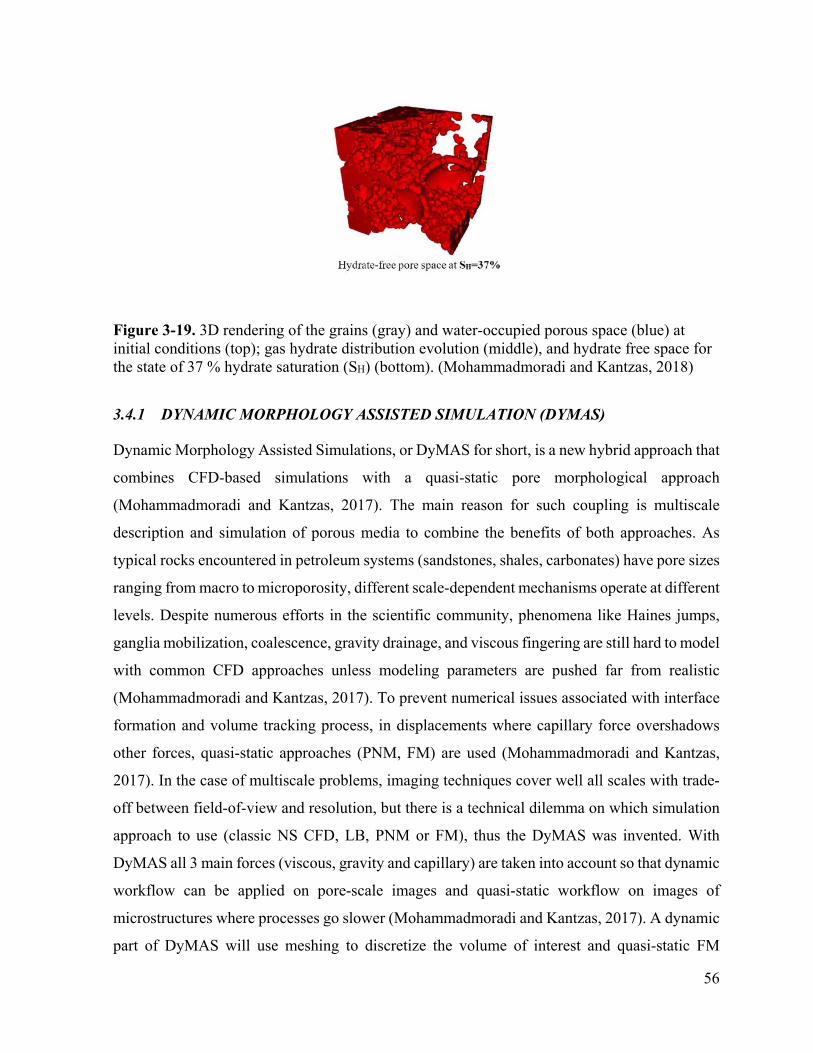
56
Figure 3-19. 3D rendering of the grains (gray) and water-occupied porous space (blue) at initial conditions (top); gas hydrate distribution evolution (middle), and hydrate free space for the state of 37 % hydrate saturation (SH) (bottom). (Mohammadmoradi and Kantzas, 2018)
3.4.1 DYNAMIC MORPHOLOGY ASSISTED SIMULATION (DYMAS)
Dynamic Morphology Assisted Simulations, or DyMAS for short, is a new hybrid approach that
combines CFD-based simulations with a quasi-static pore morphological approach
(Mohammadmoradi and Kantzas, 2017). The main reason for such coupling is multiscale
description and simulation of porous media to combine the benefits of both approaches. As
typical rocks encountered in petroleum systems (sandstones, shales, carbonates) have pore sizes
ranging from macro to microporosity, different scale-dependent mechanisms operate at different
levels. Despite numerous efforts in the scientific community, phenomena like Haines jumps,
ganglia mobilization, coalescence, gravity drainage, and viscous fingering are still hard to model
with common CFD approaches unless modeling parameters are pushed far from realistic
(Mohammadmoradi and Kantzas, 2017). To prevent numerical issues associated with interface
formation and volume tracking process, in displacements where capillary force overshadows
other forces, quasi-static approaches (PNM, FM) are used (Mohammadmoradi and Kantzas,
2017). In the case of multiscale problems, imaging techniques cover well all scales with trade-
off between field-of-view and resolution, but there is a technical dilemma on which simulation
approach to use (classic NS CFD, LB, PNM or FM), thus the DyMAS was invented. With
DyMAS all 3 main forces (viscous, gravity and capillary) are taken into account so that dynamic
workflow can be applied on pore-scale images and quasi-static workflow on images of
microstructures where processes go slower (Mohammadmoradi and Kantzas, 2017). A dynamic
part of DyMAS will use meshing to discretize the volume of interest and quasi-static FM

57
approach voxels to perform the simulations. The complete workflow of the DyMAS technique
can be seen in Figure 3-20.
Figure 3-20. DyMAS algorithm for multiscale simulation (Mohammadmoradi and Kantzas, 2017)
Moreover, Mohammadmoradi and Kantzas, 2017 stated that DyMAS is a very adaptable
technique capable of simulating classic imbibition and drainage processes, but also non-
isothermal cases with energy equation added to the simulator and minor modification in surface
tension description. As an example, a case study of SAGD (Steam Assisted Gravity Drainage)
was presented implying the potential application in EOR (Enhanced Oil Recovery) and
unconventional resources simulation. The key features of the DyMAS modeling approach are
numerical simplicity, reliability, range of application, memory expense and run time
(Mohammadmoradi and Kantzas, 2017).

58
4. CONCLUSION
To sum it all up, the goal of this thesis was to provide a review of digital rock physics with the
emphasis on the simulation of fluids in the porous media as an alternative to classical core
measurements in the lab. With all hardware novelties supported by numerous software
developments, both technical and financial factors are turning the balance in favor of digital
methods of investigation. A diversity of imaging techniques offers great flexibility in terms of
resolution. Innovative algorithms for image processing also improved capabilities of solid-void
space differentiating, particularly with the introduction of AI and machine learning. Four chosen
numerical simulation techniques were portrayed in the context of computational microfluidics.
Two out of the four techniques were characterized as dynamic and two of them as prevalently
quasi-static covering the nature of both types of processes. The first introduced was the classical
Navier-Stokes CFD approach which is also the most established technique. In favor of this
statement and as a confirmation of the efforts that the scientific community is investing in this
technique, the subchapter about OpenFOAM® and other open-source software packages was
presented. Navier-Stokes’ approach generally covers a wide range of problems and gives great
accuracy of the results. The second mentioned technique was lattice-Boltzmann, as an example
of a particle-based group of techniques. Lattice-Boltzmann's approach started gaining the
attention of researchers of the porous media mostly in the last two decades. Key features of this
technique are easy coding and the option of code parallelization which aims to reduce the run-
time of simulations. The fact that the lattice-Boltzmann technique is well known and used in
other scientific areas brings up the possibility of making correlations and analogies between the
problems. In the present moment PNM can be considered as a technique in the most advanced
state of development. Pore network models offer real simplification of the complex pore systems
present in rocks, however the simplification goes on the cost of inherited limitations which are
well understood and may be accounted for. The full pore-morphology approach is still relatively
new, unknown and fundamentally different comparing to the other techniques. Nevertheless,
the research is showing promising results. The main attributes of the full pore-morphology
approach are numerical simplicity, reliability, range of application, memory expense and run
time while at the same time being comparable to all other simulation and experimental
techniques for solving multiphase problems in porous media. In the end, the goal of numerical

59
simulations on pore scale and all mentioned research is to benefit and be applied in real-life,
large-scale engineering projects.
5. REFERENCES
1. AHRENHOLZ, B. et al. 2008. Prediction of capillary hysteresis in a porous material
using lattice-Boltzmann methods and comparison to experimental data and a
morphological pore network model, Advances in Water Resources, 31(9), pp. 1151–
1173. doi: 10.1016/j.advwatres.2008.03.009.
2. AL-RAOUSH, R. I. and WILLSON, C. S. 2005. Extraction of physically realistic pore
network properties from three-dimensional synchrotron X-ray microtomography images
of unconsolidated porous media systems, Journal of Hydrology, 300(1–4), pp. 44–64.
doi: 10.1016/j.jhydrol.2004.05.005.
3. AL-RAOUSH, R., THOMPSON, K. and WILLSON, C. S. 2003. Comparison of
Network Generation Techniques for Unconsolidated Porous Media, Soil Science Society
of America Journal, 67(6). doi: 10.2136/sssaj2003.1687.
4. ANDRÄ, H. et al. 2013. Digital rock physics benchmarks-Part I: Imaging and
segmentation, Computers and Geosciences, 50, pp. 25–32. doi:
10.1016/j.cageo.2012.09.005.
5. ANISZEWSKI, W., ARRUFAT, T. and CRIALESI-ESPOSITO, M. 2021.
Conservative Volume-of-Fluid method for free-surface simulations on Cartesian-grids,
Journal of Computational Physics, 263(8), p. 2021. doi: 10.17632/5cb2yrfx7r.1.
6. ARGANDA-CARRERAS, I. 2016. Introduction to Image Segmentation using
ImageJ/Fiji. Available at: https://imagej.net/media/arganda-carreras-segmentation-
bioimage-course-mdc-berlin-2016.pdf (Accessed: June 29, 2021).
7. ARMSTRONG, R. T. et al. 2019. Porous Media Characterization Using Minkowski
Functionals: Theories, Applications and Future Directions, Transport in Porous Media,
130(1), pp. 305–335. doi: 10.1007/s11242-018-1201-4.
8. ARRUFAT, T. et al. 2014. Developments on Relative Permeability Computation in 3D
Rock Images. Available at: http://parissimulator.sourceforge.net.
9. BAKKER, A. 2002. Lecture 5-Solution Methods Applied Computational Fluid
Dynamics. Available at: http://www.bakker.org.

60
10. BALDWIN, C. A. et al. 1996. Determination and Characterization of the Structure of
a Pore Space from 3D Volume Images, Journal of Colloid and Interface Science, 181(1).
doi: 10.1006/jcis.1996.0358.
11. BEAR, J. 1988. Dynamics of fluids in porous media. New York (N.Y.) : Dover.
Available at: http://lib.ugent.be/catalog/rug01:000487153.
12. BHATNAGAR, P. L., GROSS, E. P. and KROOK, M. 1954. A Model for Collision
Processes in Gases. I. Small Amplitude Processes in Charged and Neutral One-
Component Systems, Physical Review, 94(3). doi: 10.1103/PhysRev.94.511.
13. BIJELJIC, B. et al. 2013. Predictions of non-Fickian solute transport in different
classes of porous media using direct simulation on pore-scale images, Physical Review
E - Statistical, Nonlinear, and Soft Matter Physics, 87(1). doi:
10.1103/PhysRevE.87.013011.
14. BLUNT, M. J. et al. 2013. Pore-scale imaging and modelling, Advances in Water
Resources, 51, pp. 197–216. doi: 10.1016/j.advwatres.2012.03.003.
15. BRUNKE, O. et al. 2008. Comparison between x-ray tube-based and synchrotron
radiation-based μCT, in Stock, S. R. (ed.). doi: 10.1117/12.794789.
16. BRUNKE, O., NEUSER, E. and SUPPES, A. 2011. High Resolution Industrial CT
Systems: Advances and Comparison with Synchrotron-Based CT, Internal Symposium
on Digital Industrial Radiology and Computed Tomography, Berlin, Germany, June,
2011.
17. Cadence PCB solutions 2020. CFD Simulation Types: Discretization, Approximation,
and Algorithms. Available at: https://resources.pcb.cadence.com/blog/2020-cfd-
simulation-types-discretization-approximation-and-algorithms (Accessed: July 9,
2021).
18. CARBONELL, R. G. and WHITAKER, S. 1983. DISPERSION IN PULSED
SYSTEMS-II THEORETICAL DEVELOPM’ENTS FOR PASSIVE DISPERSION IN
POROUS MEDIA, Chtmiral EORiotenOR Sri .. ce.
19. CHAI, M. et al. 2021. Imposing mixed Dirichlet-Neumann-Robin boundary conditions
on irregular domains in a level set/ghost fluid based finite difference framework,
Computers and Fluids, 214. doi: 10.1016/j.compfluid.2020.104772.

61
20. CHAN, T. P. and GOVINDARAJU, R. S. 2011. Pore-morphology-based simulations
of drainage and wetting processes in porous media, Hydrology Research, 42(2–3), pp.
128–149. doi: 10.2166/nh.2011.058.
21. COSTABEL, M. 1986. Principles of Boundary Element Methods.
22. CRANK, J. and NICOLSON, P. 1947. A practical method for numerical evaluation of
solutions of partial differential equations of the heat-conduction type, Mathematical
Proceedings of the Cambridge Philosophical Society, 43(1), pp. 50–67. doi:
10.1017/S0305004100023197.
23. DAL FERRO, N. et al. 2015. Application of smoothed particle hydrodynamics (SPH)
and pore morphologic model 2 to predict saturated water conductivity from X-ray CT
imaging in a silty loam Cambisol. doi: 10.1016/j.geoderma.2015.04.019ï.
24. ELOTMANI, M. et al. 2016. DETECTION OF RING ARTIFACTS IN COMPUTED
TOMOGRAPHIC IMAGES, Journal of Theoretical and Applied Information
Technology, 94(1), pp. 84–94. Available at: https://hal.archives-ouvertes.fr/hal-
01998216.
25. FATT, I. 1956. The Network Model of Porous Media, Transactions of the AIME,
207(01). doi: 10.2118/574-G.
26. FELDKAMP, L. A., DAVIS, L. C. and KRESS, J. W. 1984. Practical cone-beam
algorithm, Journal of the Optical Society of America A, 1(6). doi:
10.1364/JOSAA.1.000612.
27. FERZIGER, J. H. and PERIĆ, M. 2002. Computational Methods for Fluid Dynamics.
28. GACKIEWICZ, B. et al. 2021. An intercomparison of the pore network to the Navier–
Stokes modeling approach applied for saturated conductivity estimation from X-ray CT
images, Scientific Reports, 11(1). doi: 10.1038/s41598-021-85325-z.
29. GRAVELEAU, M., SOULAINE, C. and TCHELEPI, H. A. 2017. Pore-Scale
Simulation of Interphase Multicomponent Mass Transfer for Subsurface Flow,
Transport in Porous Media, 120(2), pp. 287–308. doi: 10.1007/s11242-017-0921-1.
30. GUIBERT, R. et al. 2015a. Computational Permeability Determination from Pore-
Scale Imaging: Sample Size, Mesh and Method Sensitivities, Transport in Porous
Media, 107(3), pp. 641–656. doi: 10.1007/s11242-015-0458-0.

62
31. GUIBERT, R. et al. 2015b. Computational Permeability Determination from Pore-
Scale Imaging: Sample Size, Mesh and Method Sensitivities, Transport in Porous
Media, 107(3), pp. 641–656. doi: 10.1007/s11242-015-0458-0.
32. GUO, J., VERAN-TISSOIRES, S. and QUINTARD, M. 2016. Effective surface and
boundary conditions for heterogeneous surfaces with mixed boundary conditions,
Journal of Computational Physics, 305, pp. 942–963. doi: 10.1016/j.jcp.2015.10.050.
33. HAJIZADEH, A. and FARHADPOUR, Z. 2012. An Algorithm for 3D Pore Space
Reconstruction from a 2D Image Using Sequential Simulation and Gradual Deformation
with the Probability Perturbation Sampler, Transport in Porous Media, 94(3), pp. 859–
881. doi: 10.1007/s11242-012-0028-7.
34. HAROUN, Y., LEGENDRE, D. and RAYNAL, L. 2010. Volume of fluid method for
interfacial reactive mass transfer: Application to stable liquid film, Chemical
Engineering Science, 65(10), pp. 2896–2909. doi: 10.1016/j.ces.2010.01.012.
35. HAZLETT, R. D. 1995. Simulation of capillary-dominated displacements in
microtomographic images of reservoir rocks, Transport in Porous Media, 20(1–2). doi:
10.1007/BF00616924.
36. HEINEMANN, Z. E. et al. 1989. Modeling Reservoir Geometry with Irregular Grid.
37. HEUBES, D., BARTEL, A. and EHRHARDT, M. 2013. An Introduction to the Lattice
Boltzmann Method for Coupled Problems, in Heubes, D., Bartel, A., and Ehrhardt, M.
(eds) Progress in Computational Physics Volume 3: Novel Trends in Lattice-Boltzmann
Methods. BENTHAM SCIENCE PUBLISHERS. doi:
10.2174/9781608057160113030004.
38. HILPERT, M. and MILLER, C. T. 2001. Pore-morphology-based simulation of
drainage in totally wetting porous media, Advances in Water Resources, 24(3), pp. 243–
255. doi: https://doi.org/10.1016/S0309-1708(00)00056-7.
39. HIRSCH, C. 2007. Numerical Computation of Internal and External Flows -
Fundamentals of Computational Fluid Dynamics.
40. HORGUE, P. et al. 2015. An open-source toolbox for multiphase flow in porous media,
Computer Physics Communications, 187, pp. 217–226. doi: 10.1016/j.cpc.2014.10.005.

63
41. HUI, Z. et al. 2021. Application of Lightning Breakdown Simulation in Inversion of
Induced Fracture Network Morphology in Stimulated Reservoirs, in Day 1 Tue, March
23, 2021. IPTC. doi: 10.2523/IPTC-21157-MS.
42. JACQMIN, D. 1999. Calculation of Two-Phase Navier-Stokes Flows Using Phase-
Field Modeling, Journal of Computational Physics. Available at:
http://www.idealibrary.comon.
43. JAIN, S. et al. 2003. Monte Carlo simulation of flow of fluids through porous media,
Computers and Chemical Engineering, 27(3), pp. 385–400. doi: 10.1016/S0098-
1354(02)00211-9.
44. JASAK, H. 2009. Dynamic Mesh Handling in OpenFOAM.
45. JIANG, F. and TSUJI, T. 2017. Estimation of three-phase relative permeability by
simulating fluid dynamics directly on rock-microstructure images, Water Resources
Research, 53(1), pp. 11–32. doi: 10.1002/2016WR019098.
46. JOEKAR-NIASAR, V. and HASSANIZADEH, S. M. 2012. Analysis of Fundamentals
of Two-Phase Flow in Porous Media Using Dynamic Pore-Network Models: A Review,
Critical Reviews in Environmental Science and Technology, 42(18). doi:
10.1080/10643389.2011.574101.
47. JOHNSON, E. F., BOSSLER, D. P. and NAUMANN, V. O. 1959. Calculation of
Relative Permeability from Displacement Experiments, Transactions of the AIME,
216(01). doi: 10.2118/1023-G.
48. KETCHAM, R. A. and CARLSON, W. D. 2001. Acquisition, optimization and
interpretation of X-ray computed tomographic imagery: applications to the geosciences,
Computers & Geosciences.
49. LEE, S.-Y. and HOLDER, G. D. 2001. Methane hydrates potential as a future energy
source, Fuel Processing Technology. Available at: www.elsevier.comrlocaterfuproc.
50. LEHMANN, P. et al. 2006. Tomographical Imaging and Mathematical Description of
Porous Media Used for the Prediction of Fluid Distribution, Vadose Zone Journal, 5(1).
doi: 10.2136/vzj2004.0177.
51. LINDQUIST, W. B. and VENKATARANGAN, A. 1999. Investigating 3D geometry
of porous media from high resolution images, Physics and Chemistry of the Earth, Part
A: Solid Earth and Geodesy, 24(7). doi: 10.1016/S1464-1895(99)00085-X.

64
52. LORENSEN, W. E. and CLINE, H. E. 1987. Marching cubes: A high resolution 3D
surface construction algorithm, in Proceedings of the 14th Annual Conference on
Computer Graphics and Interactive Techniques, SIGGRAPH 1987. Association for
Computing Machinery, Inc, pp. 163–169. doi: 10.1145/37401.37422.
53. MEAKIN, P. and TARTAKOVSKY, A. M. 2009. Modeling and simulation of pore-
scale multiphase fluid flow and reactive transport in fractured and porous media,
Reviews of Geophysics. doi: 10.1029/2008RG000263.
54. MITCHELL, J., WEBBER, J. B. W. and STRANGE, J. H. 2008. Nuclear magnetic
resonance cryoporometry, Physics Reports, pp. 1–36. doi:
10.1016/j.physrep.2008.02.001.
55. MOHAMMADMORADI, P. et al. 2017. Pore Network and Morphological
Characterization of Pore-Level Structures.
56. MOHAMMADMORADI, P., BEHRANG, A. and KANTZAS, A. 2016. Effective
Thermal and Electrical Conductivity of Two-Phase Saturated Porous Media, in Day 2
Wed, June 08, 2016. SPE. doi: 10.2118/180740-MS.
57. MOHAMMADMORADI, P. and KANTZAS, A. 2017. DyMAS: A Direct Multi-Scale
Pore-Level Simulation Approach.
58. MOHAMMADMORADI, P. and KANTZAS, A. 2018. Direct geometrical simulation
of pore space evolution through hydrate dissociation in methane hydrate reservoirs,
Marine and Petroleum Geology, 89, pp. 786–798. doi:
10.1016/j.marpetgeo.2017.11.016.
59. MONAJEMI, P. and RAKHSHANDEHROO, G. 2013. Investigating Pore Network
Models as numerical tools to solve steady saturated groundwater flow, Scientia Iranica,
20, pp. 1662–1675.
60. MOUKALLED, F., MANGANI, L. and DARWISH, M. 2016. The Finite Volume
Method in Computational Fluid Dynamics. Cham: Springer International Publishing.
doi: 10.1007/978-3-319-16874-6.
61. MUKERJI, T. 2007. Linking Rock Physics and Geostatistics for Reservoir
Characterization, Petroleum Geostatistics.

65
62. NANIA, S. L. and SHAW, S. K. 2015. Analysis of fluid film behaviour using dynamic
wetting at a smooth and roughened surface, Analytical Methods, 7(17), pp. 7242–7248.
doi: 10.1039/c5ay00574d.
63. NASAR, A. M. 2016. Eulerian and Lagrangian Smoothed Particle Hydrodynamics as
Models for the Interaction of Fluids and Flexible Structures in Biomedical Flows.
64. NOETINGER, B. et al. 2016. Random Walk Methods for Modeling Hydrodynamic
Transport in Porous and Fractured Media from Pore to Reservoir Scale, Transport in
Porous Media, 115(2), pp. 345–385. doi: 10.1007/s11242-016-0693-z.
65. NOIRIEL, C. and SOULAINE, C. 2021. Pore-Scale Imaging and Modelling of
Reactive Flow in Evolving Porous Media: Tracking the Dynamics of the Fluid–Rock
Interface, Transport in Porous Media. doi: 10.1007/s11242-021-01613-2.
66. ORTEGA RAMÍREZ, M. P., OXARANGO, L. and GASTELUM STROZZI, A. 2019.
Effect of X-ray CT resolution on the quality of permeability computation for granular
soils: definition of a criterion based on morphological properties, Soil Research, 57(6).
doi: 10.1071/SR18189.
67. ORTEGA-RAMÍREZ, M. P. and OXARANGO, L. 2021. Effect of X-ray $$\mu$$CT
Resolution on the Computation of Permeability and Dispersion Coefficient for Granular
Soils, Transport in Porous Media, 137(2). doi: 10.1007/s11242-021-01557-7.
68. PARKHURST, D. and APPELO, T. 1999. User’s guide to PHREEQC version 3 - a
computer program for speciation, batch-reaction, one-dimensional transport, and inverse
geochemical calculations, Water Resources Research Investigations Report.
69. PEJIC, D. and MAINI, B. B. 2003. Three-Phase Relative Permeability of Petroleum
Reservoirs,” in All Days. SPE. doi: 10.2118/81021-MS.
70. RAMEZANI, A., STIPCICH, G. and GARCIA, I. 2016. Introduction to Computational
Fluid Dynamics by the Finite Volume Method.
71. RAMSTAD, T. et al. 2012. “Relative Permeability Calculations from Two-Phase Flow
Simulations Directly on Digital Images of Porous Rocks,” Transport in Porous Media,
94(2), pp. 487–504. doi: 10.1007/s11242-011-9877-8.
72. RUBIO, A. D., ZALTS, A. and EL HASI, C. D. 2008. “Numerical solution of the
advection-reaction-diffusion equation at different scales, Environmental Modelling and
Software, 23(1), pp. 90–95. doi: 10.1016/j.envsoft.2007.05.009.

66
73. SAXENA, N. et al. 2017. Effect of image segmentation & voxel size on micro-CT
computed effective transport & elastic properties, Marine and Petroleum Geology, 86,
pp. 972–990. doi: 10.1016/j.marpetgeo.2017.07.004.
74. SAXENA, N. et al. 2018. Imaging and computational considerations for image
computed permeability: Operating envelope of Digital Rock Physics, Advances in Water
Resources, 116, pp. 127–144. doi: 10.1016/j.advwatres.2018.04.001.
75. SAXENA, N. et al. 2021. Estimating Fluid Saturations from Capillary Pressure and
Relative Permeability Simulations Using Digital Rock, Transport in Porous Media,
136(3), pp. 863–878. doi: 10.1007/s11242-021-01543-z.
76. SCHULZ, V. P., WARGO, E. A. and KUMBUR, E. C. 2015. Pore-Morphology-Based
Simulation of Drainage in Porous Media Featuring a Locally Variable Contact Angle,
Transport in Porous Media, 107(1), pp. 13–25. doi: 10.1007/s11242-014-0422-4.
77. SILIN, D. B., JIN, G. and PATZEK, T. W. 2003. Robust Determination of the Pore
Space Morphology in Sedimentary Rocks, in All Days. SPE. doi: 10.2118/84296-MS.
78. SONG, R. et al. 2019. Comparative analysis on pore-scale permeability prediction on
micro-CT images of rock using numerical and empirical approaches, Energy Science
and Engineering, 7(6), pp. 2842–2854. doi: 10.1002/ese3.465.
79. SOULAINE, C. et al. 2016. The Impact of Sub-Resolution Porosity of X-ray
Microtomography Images on the Permeability, Transport in Porous Media, 113(1). doi:
10.1007/s11242-016-0690-2.
80. SOULAINE, C. et al. 2017. Mineral dissolution and wormholing from a pore-scale
perspective, Journal of Fluid Mechanics, 827, pp. 457–483. doi: 10.1017/jfm.2017.499.
81. SOULAINE, C. 2018. Introduction to open-source computational fluid dynamics using
OpenFOAM® technology. Cargèse. Available at:
https://www.cypriensoulaine.com/openfoam (Accessed: July 29, 2021).
82. SOULAINE, C. et al. 2021. Digital Rock Physics: computation of hydrodynamic
dispersion, Oil & Gas Science and Technology – Revue d’IFP Energies nouvelles, 76,
p. 51. doi: 10.2516/ogst/2021032.
83. SOULAINE, C., MAES, J. and ROMAN, S. 2021a. Computational Microfluidics for
Geosciences, Frontiers in Water, 3. doi: 10.3389/frwa.2021.643714.

67
84. SOULAINE, C., MAES, J. and ROMAN, S. 2021b. Computational Microfluidics for
Geosciences, Frontiers in Water, 3. doi: 10.3389/frwa.2021.643714.
85. SPITERI, E. et al. 2005. Relative-Permeability Hysteresis: Trapping Models and
Application to Geological CO2 Sequestration, in All Days. SPE. doi: 10.2118/96448-
MS.
86. SU, N. et al. 2010. Three-dimensional reconstruction of micro pore structure, in
Proceedings - 2010 International Conference on Computational and Information
Sciences, ICCIS 2010, pp. 120–123. doi: 10.1109/ICCIS.2010.332.
87. TANWAR, S. 2018. A Meshfree-Based Lattice Boltzmann Approach for Simulation
of Fluid Flows Within Complex Geometries, in. doi: 10.4018/978-1-5225-4760-
0.ch006.
88. Thermo Fisher Scientific 2021. PerGeos for Digital Rock Analysis. Available at:
https://www.thermofisher.com/fr/en/home/industrial/electron-microscopy/electron-
microscopy-instruments-workflow-solutions/3d-visualization-analysis-
software/pergeos-digital-rock-analysis.html (Accessed: June 28, 2021).
89. TRYGGVASON, G. 2017. Computational Fluid Dynamics -Theory of Partial
Differential Equations. Available at: http://www.nd.edu/~gtryggva/CFD-Course/.
90. VERRI, I. et al. 2017. Development of a Digital Rock Physics workflow for the
analysis of sandstones and tight rocks, Journal of Petroleum Science and Engineering,
156, pp. 790–800. doi: 10.1016/j.petrol.2017.06.053.
91. VITA, P. 2020. OpenFOAM. Leoben.
92. WANG, K. and KILLOUGH, J. E. 2009. A New Upscaling Method of Relative
Permeability Curves for Reservoir Simulation.
93. DA WANG, Y. et al. 2020. Physical Accuracy of Deep Neural Networks for 2D and
3D Multi-Mineral Segmentation of Rock micro-CT Images. Available at:
http://arxiv.org/abs/2002.05322.
94. WÖRNER, M. 2012. Numerical modeling of multiphase flows in microfluidics and
micro process engineering: A review of methods and applications, Microfluidics and
Nanofluidics, pp. 841–886. doi: 10.1007/s10404-012-0940-8.
95. XIONG, Q., BAYCHEV, T. G. and JIVKOV, A. P. 2016. Review of pore network
modelling of porous media: Experimental characterisations, network constructions and

68
applications to reactive transport, Journal of Contaminant Hydrology. Elsevier B.V., pp.
101–117. doi: 10.1016/j.jconhyd.2016.07.002.
96. XU, P. et al. 2013. Prediction of relative permeability in unsaturated porous media
with a fractal approach, International Journal of Heat and Mass Transfer, 64, pp. 829–
837. doi: 10.1016/j.ijheatmasstransfer.2013.05.003.
97. YANG, F. et al. 2015. Extraction of pore-morphology and capillary pressure curves of
porous media from synchrotron-based tomography data, Scientific Reports, 5(1). doi:
10.1038/srep10635.
98. YU, Z. and FAN, L. S. 2010. Lattice Boltzmann method for simulating particle-fluid
interactions, Particuology, 8(6), pp. 539–543. doi: 10.1016/j.partic.2010.07.012.
99. ZHANG, L. et al. 2019. The investigation of permeability calculation using digital core
simulation technology, Energies, 12(17). doi: 10.3390/en12173273.
100. ZHANG, PENGFEI et al. 2017. Multi-component segmentation of X-ray computed
tomography (CT) image using multi-Otsu thresholding algorithm and scanning electron
microscopy, 35(3), pp. 281–294. doi: 10.2307/90007496.
101. ZHAO, H. Q., MACDONALD, I. F. and KWIECIEN, M. J. 1994. Multi-Orientation
Scanning: A Necessity in the Identification of Pore Necks in Porous Media by 3-D
Computer Reconstruction from Serial Section Data, Journal of Colloid and Interface
Science, 162(2). doi: 10.1006/jcis.1994.1053.
102. ZHAO, Z. and ZHOU, X. P. 2019. An integrated method for 3D reconstruction model
of porous geomaterials through 2D CT images, Computers and Geosciences, 123, pp. 83–
94. doi: 10.1016/j.cageo.2018.11.012.
103. ZHENG, D. and REZA, Z. 2019. Pore-network extraction algorithm for shale
accounting for geometry-effect, Journal of Petroleum Science and Engineering, 176, pp.
74–84. doi: 10.1016/j.petrol.2019.01.046.

IZJAVA:
Izjavljujem da sam ovaj rad izradio samostalno na temelju znanja stečenih na Rudarsko-
geološko-naftnom fakultetu sužeći se navedenom literaturom.
Viktor Gredičak

KLASA: 602-04/21-01/235
URBROJ: 251-70-12-21-2
U Zagrebu, 6.9.2021.
Viktor Gredičak, student
(potpis) (potpis)
(titula, ime i prezime) (titula, ime i prezime)
(potpis) (potpis)
(titula, ime i prezime)
Oznaka: OB 8.5.-1 SRF-1-13/0 Stranica: 1/1 Čuvanje (godina) Trajno
PhD. Cyprien Soulaine
(titula, ime i prezime)
Izv.prof.dr.sc. Dalibor
Kuhinek
Prodekan za nastavu i studente:
OBRAZAC SUSTAVA UPRAVLJANJA KVALITETOM
Na temelju vašeg zahtjeva primljenog pod KLASOM 602-04/21-01/235, URBROJ: 251-70-12-21-1 od
6.9.2021. priopćujemo vam temu diplomskog rada koja glasi:
PORE-MORPHOLOGY BASED SIMULATIONS IN POROUS MEDIA
RJEŠENJE O ODOBRENJU TEME
Voditelj:
Izv.prof.dr.sc. Luka Perković Izv.prof.dr.sc. Vladislav Brkić
Za voditelja ovog diplomskog rada imenuje se u smislu Pravilnika o izradi i obrani diplomskog rada
Izv.prof.dr.sc. Luka Perković nastavnik Rudarsko-geološko-naftnog-fakulteta Sveučilišta u Zagrebu i
suvoditelja PhD. Cyprien Soulaine.
Predsjednik povjerenstva za
završne i diplomske ispite:
Suvoditelj


![Effect of the morphology and pore structure of porous ... · agents, cigarette smoke or building materials [2]. With the increasing concerns about the IAQ, different methods have](https://img.pdfslide.net/doc/110x75/5ede588dad6a402d6669aaf7/effect-of-the-morphology-and-pore-structure-of-porous-agents-cigarette-smoke.jpg)