Louisiana State UniversityLSU Digital Commons

LSU Doctoral Dissertations Graduate School

2014

Poroelastic Inhomogeneities: Applications inReservoir GeomechanicsHouman BedayatLouisiana State University and Agricultural and Mechanical College

Follow this and additional works at: https://digitalcommons.lsu.edu/gradschool_dissertations

Part of the Petroleum Engineering Commons

This Dissertation is brought to you for free and open access by the Graduate School at LSU Digital Commons. It has been accepted for inclusion inLSU Doctoral Dissertations by an authorized graduate school editor of LSU Digital Commons. For more information, please contactgradetd@lsu.edu.

Recommended CitationBedayat, Houman, "Poroelastic Inhomogeneities: Applications in Reservoir Geomechanics" (2014). LSU Doctoral Dissertations. 1803.https://digitalcommons.lsu.edu/gradschool_dissertations/1803

POROELASTIC INHOMOGENEITIES:

APPLICATIONS IN RESERVOIR GEOMECHANICS

A Dissertation

Submitted to the Graduate Faculty of theLouisiana State University and

Agricultural and Mechanical Collegein partial fulfillment of the

requirements for the degree ofDoctor of Philosophy

in

Craft & Hawkins Department of Petroleum Engineering

byHouman Bedayat

B.S., Sharif University of Technology, 2007M.S., Sharif University of Technology, 2010

December 2014

©Copyright by Houman Bedayat, 2014All Rights Reserved

ii

To may parents Ziba and Mahmoud

To my brothers Babak and Arash

&

To my forever love Paria

iii

Acknowledgments

This dissertation could not have been completed without the great support that I have

received from so many people over the years. I wish to offer my most genuine thanks to the

following people.

To my advisor, Dr. Arash Dahi Taleghani. I would like to express my deepest gratitude to

you. The door to your office was always open whenever I had a question about my research.

I am indebted for your constant assistance, encouragement and guidance throughout my

doctoral studies. Besides being my advisor,you are a good friend and I hope to have the

opportunity to work with you in the future again.

To Dr. Yuri A. Antipov. For your help and support and invaluable guidance throughout

the research.

To Dr. George Z. Voyiadjis. For your invaluable support. Your great personality is

cherished by me as well as all your other students. Thank you for accepting to be in my

committee.

To Dr. Karsten E. Thompson. For your comments and feedbacks and for being supportive

as the chairman of the department. You will constantly remind me one of the greatest

teachers throughout my life.

To Dr. Michael J. Martin and Dr. Shahab Mehraeen. For being in my committee and

your time and kind helps.

To the great faculty and friendly staff of PETE department at LSU, Dr. John Rogers

Smith, Dr. Richard Hughes, Dr. Mayank Tyagi, Dr. Christopher White, Dr. Dandina Rao,

iv

Andi Donmyer, Janet Dugas, Fenelon Nunes, and George Ohrberg. Special thanks to Dr.

Hughes Family for their very memorable thanksgiving dinner parties!

To my favorite authors, Dr. Emmanuel Detournay, Dr. Alexander H.-D. Cheng and Dr.

John Rudnicki. I learned a lot from your publications.

To American Association of Drilling Engineers (AADE), GDL Foundation, Petroleum

Engineering Department at LSU for your financial supports.

To my officemates. Through the years I was blessed with the greatest officemates, Wei

Wang, Siyamak Rostami, Denis Klimenko, Ping Puyang, Miguel Gonzalez-Chavez, Milad

Ahmadi, Chennv Fan, Negar Dahi, Juan Felipe Bautista, Mohammad Riyami, Louise M.

Smith, Abiola Olabode, Doguhan Yilmaz, Amir Shojaei, Mustafa Hakan Ozyurtkan, and

Mohamed Abdelrahim.

To my colleagues in PETE department. Thank you all for being a great friends. Ali

Takbiri, Amin Gharabati, Masoud Safari, Reza Rahmani, Azadeh Kafili, Ali Reza Edrisi,

Alireza Roostapour, Koray Kinic, Paulina Mwangi, Lawrence Dickerson, Atheer Al Attar,

Foad Haeri, Darko Kupresan, Amin Mirsaeidi, Esmaeil Ansari and Kahila Mokhtari.

To my friends in Baton Rouge. Life in Baton Rouge would have been unbearable without

you whom I will revere forever. My friends; Ashkan, Azadeh, Nima, Fatemeh, Ali, Kasra,

Raysan, Navid, Amirhossein, Sima, Yahya, Roghayeh, Hamidreza, Mohammad, Ehsan, Af-

shin, Jafar, Arian, Navid, Mohammad, Ali, Saman, Mahan, Samira, Parvaneh, Mahzad,

Misagh, Bruce, Debby, Vahid, Sareh, Sara, Fariborz, Maryam, Ava, Ata, Kristen, Pouya,

Saaed, Houman. To my roommates; Ali, Amenda, and Tracy. To the members of Iranian

Association at LSU; especially Somayeh, Mohsen, Naim and Parichehr.

To my lovely Mother. You mean the world to me, but I don’t tell you enough. This one

is for you مامان جان !

To my Father. You sacrificed your life for my brothers and myself and provided uncon-

ditional love and care. I would not have made it this far without you. Thank you جانبابا !

v

To my brothers, Babak & Arash. You are the people who I trust the most in my life. To

their family arinaz, Layli & Ario. Thank you for your kindness.

To Uncle Mahmoud, Aunt Farideh, Haley, Mehrak, Alireza, Amir, Shaliz & their lovely

kids. Thank you for all your support.

To my fiancee, Paria. I am lucky to have you in my life. I love you, and look forward to

our lifelong journey.

To many great people and places in Baton Rouge. Dr. Aghazadeh, CEBA, Union,

Starbucks, Perkin’s Rowe, Kona Grill, Hamid Agha, Almazze, Agha Mehdi, Agha Nader,

Marguerite Prince Acosta, Acha Bakery, Quad, Health center, Lady of the Lake, Embassy

Apartments, and Louisiana fire ants!.

To anyone that may I have forgotten. I apologize. Thank you as well.

vi

Table of Contents

Acknowledgments . . . . . . . . . . . . . . . . . . . . . . . . . . . . . . . . . . . . . iv

List of Tables . . . . . . . . . . . . . . . . . . . . . . . . . . . . . . . . . . . . . . . . x

List of Figures . . . . . . . . . . . . . . . . . . . . . . . . . . . . . . . . . . . . . . . xi

Abstract . . . . . . . . . . . . . . . . . . . . . . . . . . . . . . . . . . . . . . . . . . xv

1 Overview . . . . . . . . . . . . . . . . . . . . . . . . . . . . . . . . . . . . . . . . 11.1 Introduction . . . . . . . . . . . . . . . . . . . . . . . . . . . . . . . . . . . . 11.2 Outline . . . . . . . . . . . . . . . . . . . . . . . . . . . . . . . . . . . . . . . 31.3 References . . . . . . . . . . . . . . . . . . . . . . . . . . . . . . . . . . . . . 5

2 Interacting Double Poroelastic Inclusions . . . . . . . . . . . . . . . . . . . . . . 72.1 Introduction . . . . . . . . . . . . . . . . . . . . . . . . . . . . . . . . . . . . 72.2 Single Inclusion . . . . . . . . . . . . . . . . . . . . . . . . . . . . . . . . . . 11

2.2.1 Elastic inclusions . . . . . . . . . . . . . . . . . . . . . . . . . . . . . 112.2.2 Poroelastic inclusions . . . . . . . . . . . . . . . . . . . . . . . . . . . 12

2.3 Two Inclusions . . . . . . . . . . . . . . . . . . . . . . . . . . . . . . . . . . 142.4 Results and Discussions . . . . . . . . . . . . . . . . . . . . . . . . . . . . . 182.5 Summary . . . . . . . . . . . . . . . . . . . . . . . . . . . . . . . . . . . . . 212.6 Polynomial Eigenstrains . . . . . . . . . . . . . . . . . . . . . . . . . . . . . 242.7 References . . . . . . . . . . . . . . . . . . . . . . . . . . . . . . . . . . . . . 27

3 On the Inhomogeneous Anisotropic Poroelastic Inclusions . . . . . . . . . . . . . 313.1 Introduction . . . . . . . . . . . . . . . . . . . . . . . . . . . . . . . . . . . . 313.2 Anisotropic poroelastic constitutive equations . . . . . . . . . . . . . . . . . 363.3 Eshelby’s solution . . . . . . . . . . . . . . . . . . . . . . . . . . . . . . . . . 373.4 Poroelastic Inclusions . . . . . . . . . . . . . . . . . . . . . . . . . . . . . . . 403.5 Results and Discussions . . . . . . . . . . . . . . . . . . . . . . . . . . . . . 413.6 Conclusion . . . . . . . . . . . . . . . . . . . . . . . . . . . . . . . . . . . . . 473.7 Calculating Dijkl . . . . . . . . . . . . . . . . . . . . . . . . . . . . . . . . . 483.8 Results for Ellipsoidal Isotropic Poroelastic Inclusion . . . . . . . . . . . . . 493.9 A Discussion on the Effective Material Properties of the Medium . . . . . . . 503.10 References . . . . . . . . . . . . . . . . . . . . . . . . . . . . . . . . . . . . . 54

4 Eshelby Solution for Double Ellipsoidal Inhomogeneities: Applications in Geoscience 66

vii

4.1 Introduction . . . . . . . . . . . . . . . . . . . . . . . . . . . . . . . . . . . . 664.2 Theory . . . . . . . . . . . . . . . . . . . . . . . . . . . . . . . . . . . . . . . 68

4.2.1 Single inclusion . . . . . . . . . . . . . . . . . . . . . . . . . . . . . . 684.2.2 Single inhomogeneity . . . . . . . . . . . . . . . . . . . . . . . . . . . 694.2.3 Double interacting inclusions . . . . . . . . . . . . . . . . . . . . . . . 70

4.3 Formulation . . . . . . . . . . . . . . . . . . . . . . . . . . . . . . . . . . . . 714.4 Description of the Mathematica code . . . . . . . . . . . . . . . . . . . . . . 744.5 Verification and Numerical results . . . . . . . . . . . . . . . . . . . . . . . . 754.6 Conclusion . . . . . . . . . . . . . . . . . . . . . . . . . . . . . . . . . . . . . 804.7 Supplementary data . . . . . . . . . . . . . . . . . . . . . . . . . . . . . . . 804.8 Double inhomogeneity problem . . . . . . . . . . . . . . . . . . . . . . . . . 804.9 Detailed formulation of Eshelby tensor D . . . . . . . . . . . . . . . . . . . . 834.10 References . . . . . . . . . . . . . . . . . . . . . . . . . . . . . . . . . . . . . 87

5 Drainage of Poroelastic Fractures and Its Implications on the Performance ofNaturally Fractured Reservoirs . . . . . . . . . . . . . . . . . . . . . . . . . . . . 915.1 Introduction . . . . . . . . . . . . . . . . . . . . . . . . . . . . . . . . . . . . 925.2 Statement of the Problem & Assumptions . . . . . . . . . . . . . . . . . . . 975.3 Governing Equations . . . . . . . . . . . . . . . . . . . . . . . . . . . . . . . 98

5.3.1 Mode decomposition . . . . . . . . . . . . . . . . . . . . . . . . . . . 1005.3.2 Fundamental solutions . . . . . . . . . . . . . . . . . . . . . . . . . . 102

5.4 Results and Discussions . . . . . . . . . . . . . . . . . . . . . . . . . . . . . 1045.4.1 Numerical results . . . . . . . . . . . . . . . . . . . . . . . . . . . . . 105

5.5 Conclusion . . . . . . . . . . . . . . . . . . . . . . . . . . . . . . . . . . . . . 1105.6 References . . . . . . . . . . . . . . . . . . . . . . . . . . . . . . . . . . . . . 110

6 Pressurized Poroelastic Inclusions: Short-term and Long-term Asymptotic Solutions1156.1 Introduction . . . . . . . . . . . . . . . . . . . . . . . . . . . . . . . . . . . . 1166.2 Solution Methods . . . . . . . . . . . . . . . . . . . . . . . . . . . . . . . . . 118

6.2.1 General approach . . . . . . . . . . . . . . . . . . . . . . . . . . . . . 1186.2.2 Governing equations of poroelastic medium . . . . . . . . . . . . . . . 1196.2.3 Poroelastic inclusions . . . . . . . . . . . . . . . . . . . . . . . . . . . 121

6.3 Asymptotic Analysis . . . . . . . . . . . . . . . . . . . . . . . . . . . . . . . 1226.3.1 Mode (1) loading . . . . . . . . . . . . . . . . . . . . . . . . . . . . . 1226.3.2 Mode (2) loading . . . . . . . . . . . . . . . . . . . . . . . . . . . . . 125

6.4 Numerical Results . . . . . . . . . . . . . . . . . . . . . . . . . . . . . . . . . 1266.5 Summary and Conclusion . . . . . . . . . . . . . . . . . . . . . . . . . . . . 1276.6 Diffusion equation solution on an ellipsoidal surface . . . . . . . . . . . . . . 1306.7 Duhamel’s theorem . . . . . . . . . . . . . . . . . . . . . . . . . . . . . . . . 1326.8 References . . . . . . . . . . . . . . . . . . . . . . . . . . . . . . . . . . . . . 133

7 Summary and Future Works . . . . . . . . . . . . . . . . . . . . . . . . . . . . . 1357.1 Summary . . . . . . . . . . . . . . . . . . . . . . . . . . . . . . . . . . . . . 1357.2 Recommendations for Future Works . . . . . . . . . . . . . . . . . . . . . . . 138

viii

Appendix: Letters of Permission to Use Published Material . . . . . . . . . . . . . . 139

Vita. . . . . . . . . . . . . . . . . . . . . . . . . . . . . . . . . . . . . . . . . . . . . . . . . . . . . . . . . . . . . . . 142

ix

List of Tables

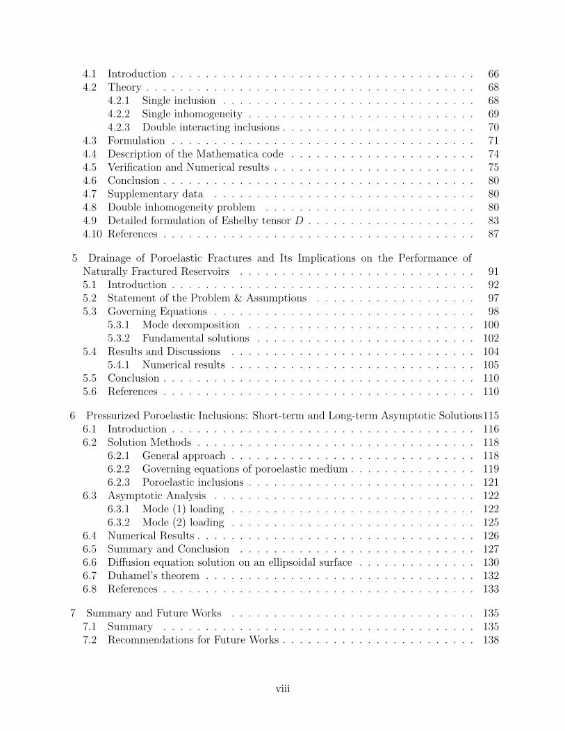
5.1 Different example descriptions for numerical analysis . . . . . . . . . . . . . 105

5.2 Input parameters . . . . . . . . . . . . . . . . . . . . . . . . . . . . . . . . . 106

6.1 The analogy between heat conduction and fluid diffusion equations . . . . . 130

6.2 Dimensionless conduction shape factors and blending coefficients for differentgeometries (from Yovanovich et al. (1995)) . . . . . . . . . . . . . . . . . . . 132

x

List of Figures

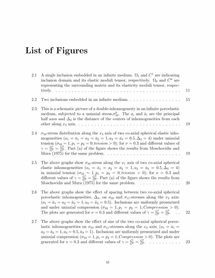
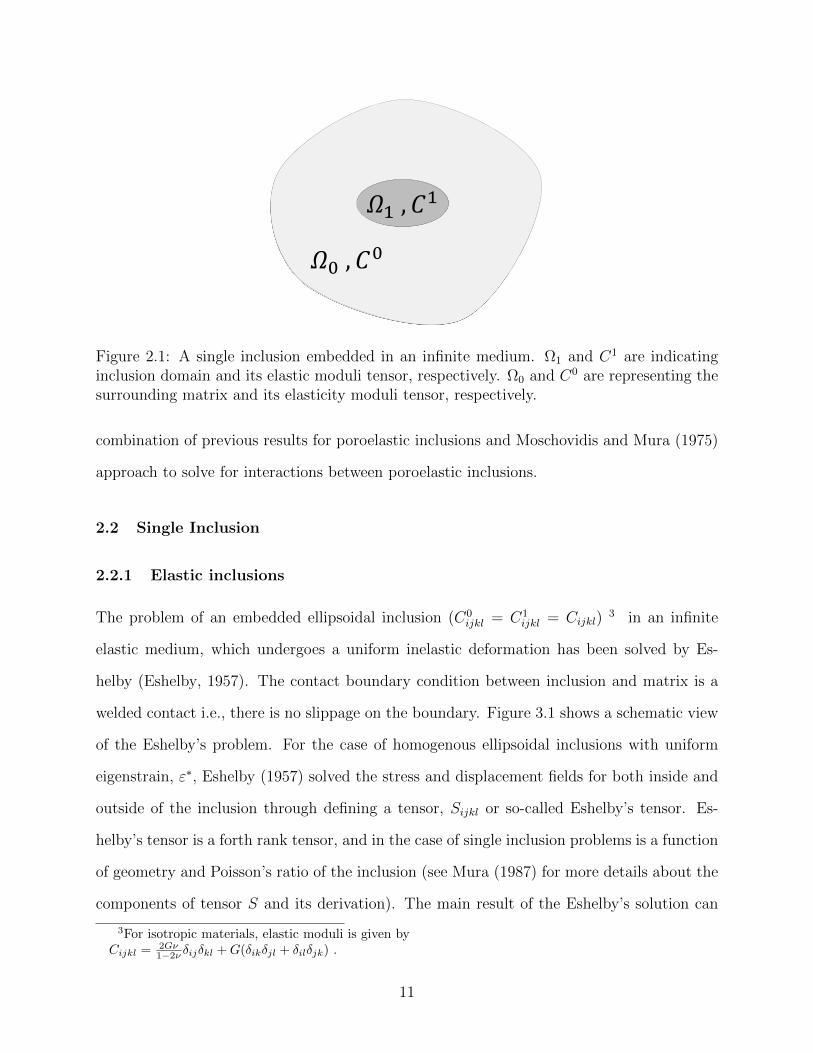
2.1 A single inclusion embedded in an infinite medium. Ω1 and C1 are indicatinginclusion domain and its elastic moduli tensor, respectively. Ω0 and C0 arerepresenting the surrounding matrix and its elasticity moduli tensor, respec-tively. . . . . . . . . . . . . . . . . . . . . . . . . . . . . . . . . . . . . . . . 11

2.2 Two inclusions embedded in an infinite medium. . . . . . . . . . . . . . . . . 15

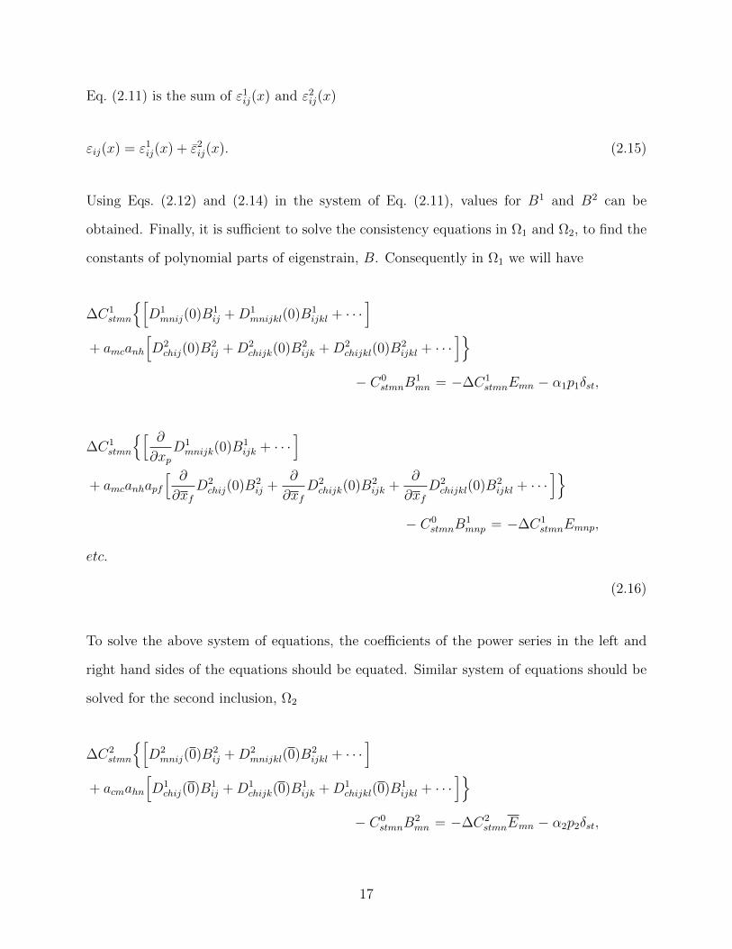
2.3 This is a schematic picture of a double-inhomogeneity in an infinite poroelasticmedium, subjected to a uniaxial stress,σ0

33. The ai and ai are the principalhalf axes and ∆3 is the distance of the centers of inhomogeneities from eachother along x3 axis. . . . . . . . . . . . . . . . . . . . . . . . . . . . . . . . . 19

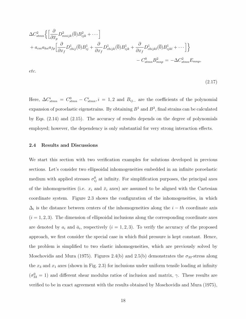
2.4 σ33-stress distribution along the x3 axis of two co-axial spherical elastic inho-mogeneities (a1 = a1 = a2 = a2 = 1, a3 = a3 = 0.5,∆3 = 4) under uniaxialtension (σ33 = 1, p1 = p2 = 0; tension > 0); for ν = 0.3 and different values ofγ = G1

G0 = G2

G0 . Part (a) of the figure shows the results from Moschovidis andMura (1975) for the same problem. . . . . . . . . . . . . . . . . . . . . . . . 19

2.5 The above graphs show σ33-stress along the x1 axis of two co-axial sphericalelastic inhomogeneities (a1 = a1 = a2 = a2 = 1, a3 = a3 = 0.5,∆3 = 4)in uniaxial tension (σ33 = 1, p1 = p2 = 0; tension > 0); for ν = 0.3 anddifferent values of γ = G1

G0 = G2

G0 . Part (a) of the figure shows the results fromMoschovidis and Mura (1975) for the same problem. . . . . . . . . . . . . . 20

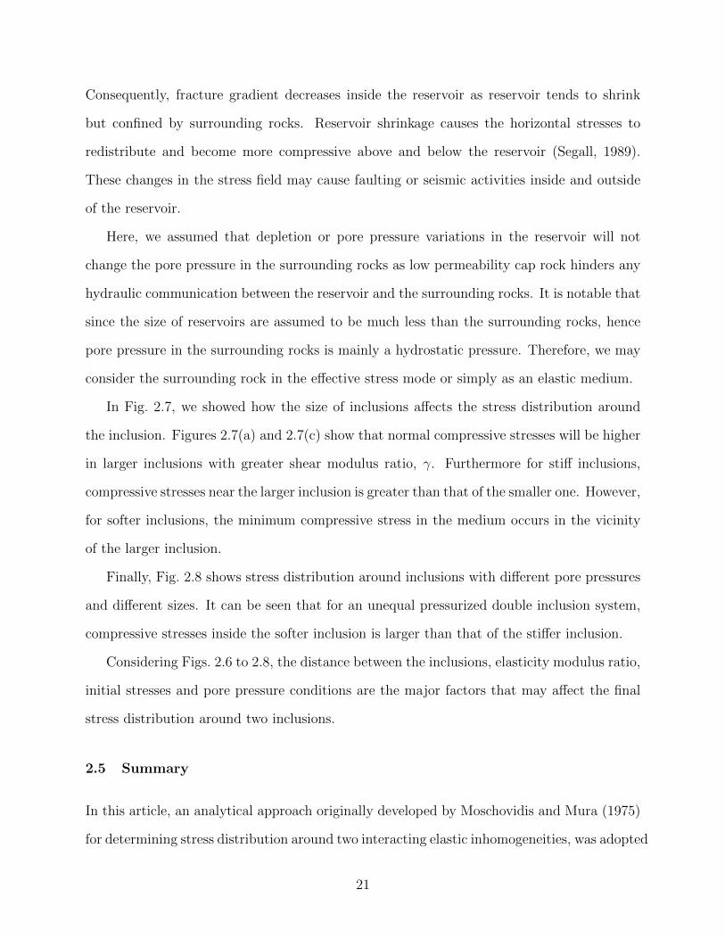
2.6 The above graphs show the effect of spacing between two co-axial sphericalporoelastic inhomogeneities, ∆3, on σ33 and σ11-stresses along the x3 axis;(a1 = a1 = a2 = a2 = 1, a3 = a3 = 0.5). Inclusions are uniformly pressurizedand under uniaxial compression (σ33 = 1, p1 = p2 = 1;Compression > 0).The plots are generated for ν = 0.3 and different values of γ = G1

G0 = G2

G0 . . . 22

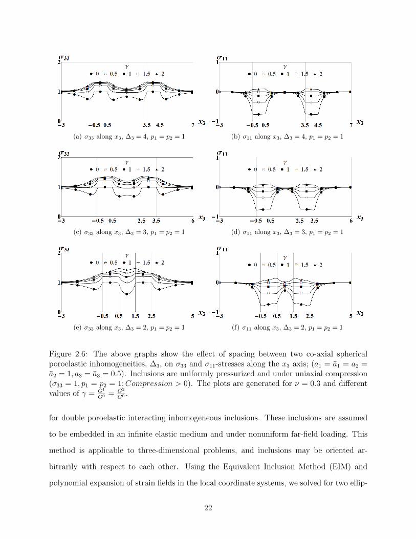
2.7 The above graphs show the effect of size of the two co-axial spherical poroe-lastic inhomogeneities on σ33 and σ11-stresses along the x3 axis; (a1 = a1 =a2 = a2 = 1, a3 = 0.5, a3 = 1). Inclusions are uniformly pressurized and underuniaxial compression (σ33 = 1, p1 = p2 = 1;Compression > 0). The plots aregenerated for ν = 0.3 and different values of γ = G1

G0 = G2

G0 . . . . . . . . . . . 23

xi

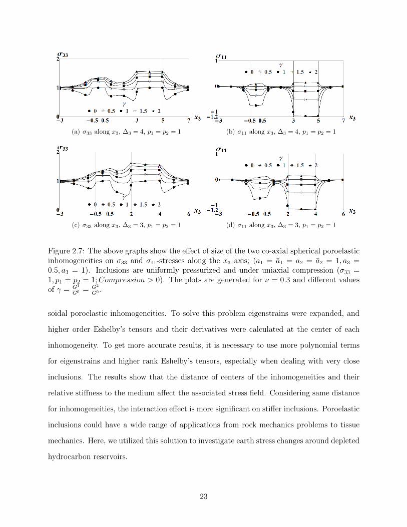
2.8 The above graphs show the effect of different pressure values inside the the twoco-axial spherical poroelastic inhomogeneities on σ33 and σ11-stresses alongthe x3 axis; (a1 = a1 = a2 = a2 = 1, a3 = a3 = 0.5). Inclusions are uni-formly pressurized and under uniaxial compression (σ33 = 1, p1 = 1, p2 =2;Compression > 0). The plots are generated for ν = 0.3 and differentvalues of γ = G1

G0 = G2

G0 . . . . . . . . . . . . . . . . . . . . . . . . . . . . . . . 24

3.1 A single inclusion embedded in an infinite medium. Ω∗ and C∗ are indicatinginclusion domain and its elastic moduli tensor, respectively. Ω and C are rep-resenting the surrounding matrix and its elasticity moduli tensor, respectively. 38

3.2 (a) Strain ratio; (b) Stress ratio due to pressure change inside an isotropicporoelastic inhomogeneity. Both graphs are plotted against the inhomogeneityaspect ratio, e. It is assumed g is shear modulus ratio, G∗/G; αij = δij(isotropic case); and ν0 = ν∗ = 0.2. However, the dependence of the solutionon ν0 is weak. These graphs are in exact agreement with Figs. 4 and 7 inRudnicki (2002a). . . . . . . . . . . . . . . . . . . . . . . . . . . . . . . . . . 41

3.3 A schematic figure of transversely isotropic material. Planes parrel to x − yare the planes of isotropy. . . . . . . . . . . . . . . . . . . . . . . . . . . . . 42

3.4 Stress ratio against inhomogeneity aspect ratio, e, for various shear modulusratio (g = G∗/G0) and Poisson’s ratio. The solid lines indicate vertical stressratio σ33/p, whereas the dotted lines indicate lateral stress ratio σ11/p. . . . 45

3.5 Stress ratio for different α33 values. g = G∗

G0 ; ν0 = ν∗ = 0.2; a1 = a2 = a3 = 1.(a) σ33/p if α33 = 0.1; (b) σ33/p if α33 = 1; (c)σd33/p, difference of part (a) and(b); (d) σ11/p if α33 = 0.1; (e) σ11/p if α33 = 1; (f)σd11/p, difference of part (d)and (e). . . . . . . . . . . . . . . . . . . . . . . . . . . . . . . . . . . . . . . 46

3.6 Vertical stress ratio σ33/p versus (a) horizontal (b) vertical distance from theinhomogeneity center due to pressure change inside the poroelastic inhomo-geneity, for different elastic and poroelastic anisotropic cases. Solid lines showtransverse isotropic case; dashed lines show isotropic elastic case. For theisotropic case we assumed ν0 = ν∗ = 0.2, g = 1, a1 = a2 = a3 = 1; Fortransverse isotropic case we used the results reported by (Pena, 1998, pp.33) for saturated sandstone cores from an oil reservoir in Budare, Venezuela(c11 = 3.6, c33 = 3.32, c44 = 0.99, c66 = 1.19, c12 = 1.29, c13 = 1.28). . . . . . 47

3.7 A medium consisted of pressurized poroelastic unidirectionally aligned inclu-sions embedded in an elastic matrix . . . . . . . . . . . . . . . . . . . . . . . 51

xii

3.8 Longitudinal Young’s modulus of the medium (E11)M to Young’s modulus ofthe matrix Em for σ0

11 = 1 and p = 1 and different inhomogeneity aspect ratiosR, and volume ratios β for different material properties ratio of the inhomo-geneities and the matrix (a) EI/Em = 0.1 (b) EI/Em = 1.0 (c) EI/Em = 2.0;(d) different p/σ0

11 ratios . . . . . . . . . . . . . . . . . . . . . . . . . . . . . 55

4.1 An ellipsoidal inclusion with principal axis parallel to Cartesian coordinatesystem (x1, x2, x3) . . . . . . . . . . . . . . . . . . . . . . . . . . . . . . . . . 69

4.2 Two ellipsoidal inhomogeneities . . . . . . . . . . . . . . . . . . . . . . . . . 71

4.3 (a, b) σ11 and σ33 vs x1, for a single void inhomogeneity for various values ofa3/a2, compare with Meng et al. (2012) and Healy (2009); (c) σ33 vs a2/a1 foran ellipsoidal inhomogeneity for various values of g = G∗

G0 , compare with Mura(1987). . . . . . . . . . . . . . . . . . . . . . . . . . . . . . . . . . . . . . . . 76

4.4 Stress vs x3 for two interacting ellipsoidal cavities with uniform unit internalpressure, compare with Moschovidis (1975). . . . . . . . . . . . . . . . . . . 77

4.5 (a) Schematic of an ellipsoidal inhomogeneity which models pore pressurechanges in a reservoir. This model calculates stress distribution inside andoutside of the reservoir, due to pore pressure changes inside the reservoirs.(b) Changes in σ11 = σ22 vs x3 (c) changes in σ33 vs x3 due to unit pressuredrop inside the reservoir. It is assumed g1 = G∗

G0 = 0.5 and a2/a1 = 1,a1/a3 = 3. x3 = 0 is center of the inhomogeneity. . . . . . . . . . . . . . . . 78

4.6 (a) Schematic of two ellipsoidal inhomogeneities which models pore pressurechanges in two adjacent reservoirs. This model calculates stress distributioninside and outside of two adjacent reservoir, due to pore pressure changesinside the reservoirs. (b) Changes in σ11 = σ22 vs x3 (c) changes in σ33 vsx3 due to unit pressure drop inside two adjacent reservoirs. It is assumedg1 = g2 = G∗

G0 = 0.5 and a2/a1 = 1, a1/a3 = 3. x3 = 0 and x3 = −3 are centersof the two ellipsoidal inhomogeneities. . . . . . . . . . . . . . . . . . . . . . . 79

5.1 Aperture size distribution in Groove Creek and Kinlaw formations followpower-law relations. Micro-fractures occur much more frequently than largesize fractures (Gale, 2002). . . . . . . . . . . . . . . . . . . . . . . . . . . . . 94

5.2 The schematic picture for a single crack in an infinite poroelastic medium. . 98

5.3 Volume changes of a single fracture due to production in a low confining stressversus dimensionless time. . . . . . . . . . . . . . . . . . . . . . . . . . . . . 107

5.4 Volume changes of a fracture due to production under large confining stressesversus dimensionless time. . . . . . . . . . . . . . . . . . . . . . . . . . . . . 108

xiii

5.5 Volume changes of a fracture due to production under large confining stressesversus dimensionless time. . . . . . . . . . . . . . . . . . . . . . . . . . . . . 109

5.6 Volume changes of a fracture due to production under large confining stressesversus dimensionless time. . . . . . . . . . . . . . . . . . . . . . . . . . . . . 109

6.1 An ellipsoidal poroelastic inclusion with principal axes (a1, a2, a3) along majorCartesian coordinate system axis. The fluid pore pressure inside the inclusionand the matrix are pI and p0, respectively (pI > p0). . . . . . . . . . . . . . . 117

6.2 (a) Mode 2 leak-off volume ratio (b) Mode 1 volume change ratio (c) Mode2 volume change ratio; for different inclusion ratios. The material propertiesare assumed to be ν = 0.2, νu = 0.4, α = 0.89 and B = 0.8. . . . . . . . . . . 128

6.3 (a) Mode 2 leak-off volume ratio (b) Mode 1 volume change ratio (c) Mode 2volume change ratio; assuming R = 10, and for different undrained Poisson’sratios . The material properties are assumed to be ν = 0.2, α = 1. . . . . . . 129

xiv

Abstract

The scarce amount of conventional hydrocarbon reservoirs and increase of fuel consumption

in the world have made production from unconventional hydrocarbon resources inevitable.

Because of the low permeability of unconventional formations, fractures are the main paths

for the fluid to flow. Therefore, detailed knowledge of the size, orientation, and permeability

of the fracture systems are essential for reservoir engineers. Permeability of the fractures

is function of their volume and opening, and stress and fluid pore pressure distribution in

the formation. Since reservoir pressure may change over the production life of the reservoir,

studying stress redistribution and mechanical behavior of the reservoirs due to the fluid

pressure alteration plays a critical role in successfully operating the hydrocarbon fields.

This research investigates the behavior of poroelastic inclusions or inhomogeneities due to

the pore pressure change, with applications in reservoir geomechanics. Considering different

material properties and different pressure/temperature of hydrocarbon bearing formations

in comparison to those of the surrounding geological structures, hydrocarbon reservoirs and

subsurface fractures can be considered as inhomogeneities embedded inside an infinite poroe-

lastic medium. Moreover, elliptic fractures are special cases of ellipsoidal inhomogeneities

when their elastic moduli are zero, and one of the principal axes of the ellipsoid approaches

zero.

This dissertation is concerned with these two topics: the thorough study of poroelastic

inclusions and their applications in reservoir geomechanics; and poroelastic fractures and

their implications on the performance of hydrocarbon reservoirs. Analytical solutions for

xv

applied stress and strain distribution around single and double inhomogeneous poroelastic

inclusions due to pore pressure changes in inclusions are derived, using Eshelby Equivalent

Method (EIM) and assuming no hydraulic communication between the inclusion and the

surrounding medium. This assumption is reasonable for modeling situations with large

discrepancy between the permeability of the inclusion and the matrix. Later, considering

hydraulic communication between the inclusion and the matrix, solution for the volume

change of ellipsoidal poroelastic inclusions are derived.

xvi

Chapter 1Overview

1.1 Introduction

The scarce amount of conventional hydrocarbon reservoirs and increase of fuel consumption

in the world have made production from unconventional hydrocarbon resources inevitable.

North America in particular has experienced a considerable increase in share of unconven-

tional resources to the total energy needs in the last two decades (MIT, 2011; OPEC, 2011).

Energy demand is projected to increase by 41% between 2012 and 2035, with growth averag-

ing 1.5% per annum. The corresponding rising supply to meet the demand growth will come

primarily from unconventional sources, by nonOPEC members, and is expected to increase

by 10.8 MBD. United States, will provide the largest increments of non-OPEC supply, 3.6

MBD, during this period (BP, 2014).

Large volumes of these unconventional hydrocarbon resources are stored in tight naturally

fractured reservoirs, such as tight sand, shale gas, shale oil and oil shale reservoirs (Holditch

and Ephen, 2006; MIT, 2011). Because of the low permeability of these tight formations,

fractures are the main paths for the fluid to flow. In other words, fractures and their

distribution determine overall permeability of the reservoir. Fractures are of paramount

importance for economic production from naturally fractured reservoirs and in their absence,

it is impossible to recover hydrocarbons from these reservoirs (Aguilera, 2008). Therefore,

detailed knowledge of the size, orientation, and permeability of the fracture systems are

essential for reservoir engineers.

1

On the other hand, the stress regime acting in a reservoir is one of the most important

parameters which controls the permeability of the fractured reservoirs. When depletion or

injection occurs, fluid pressure in the reservoir changes, which can lead to stress changes

in the formation. Length, aperture, and permeability of the fractures in the reservoir are

function of the stress distribution in the formation. Moreover, having the knowledge of stress

variations in a reservoir, has significant application in well bore stability and drilling wells in

depleted zones. Since reservoir pressure may change frequently over the life of hydrocarbon

fields, studying stress distribution and mechanical behavior of the reservoirs due to the fluid

pressure alteration plays a critical role in successfully operating the hydrocarbon fields.

This research investigates the behavior of poroelastic inclusions (or inhomogeneities) due

to change of the pore pressure, with concentration in the applications in reservoir geome-

chanics. An inclusion is defined as a finite sub-volume of a medium, which can be classified as

inhomogeneities, homogeneous inclusions, or inhomogeneous inclusions. An inhomogeneity

is a sub-volume of a medium, which has different material properties from the surround-

ing medium. Although homogeneous inclusions have the same material properties as their

surroundings, they may possess different strain status. Inhomogeneous inclusions are finite

sub-volumes of a medium, which are made of different materials and may experience different

strain status at the same time.

Considering different material properties and different pressure/temperature of hydro-

carbon bearing formations in comparison to those of the surrounding geological structures,

hydrocarbon reservoirs and subsurface fractures can be considered as inhomogeneities em-

bedded inside an infinite poroelastic medium. Moreover, elliptic fractures are special cases

of ellipsoidal inhomogeneities when their elastic moduli are zero, and one of the principal

axes of the ellipsoid approaches zero. The fact that most rocks, to some extent, are fractured

makes studying poroelastic inhomogeneities interesting for petroleum engineers.

2

1.2 Outline

This dissertation is concerned with these two topics: the thorough study of poroelastic

inclusions and their applications in reservoir geomechanics; and poroelastic fractures and

their implications on the performance of hydrocarbon reservoirs.

In Chapter 2, an analytical solution for applied stress and strain distribution around

double inhomogeneous poroelastic inclusions due to pore pressure changes in inclusions is

provided. To address the problem, an approximate analytical approach used for elastic inclu-

sions is modified for poroelastic inclusions. An application of this model in analyzing earth

stress changes around hydrocarbon reservoirs due to fluid withdrawal/injection is discussed

at the end of the chapter. This chapter is a modified text from Bedayat and Dahi Taleghani

(2013, 2014).

In Chapter 3, the anisotropic poroelastic properties of the rocks and their impact on the

stress changes due to pore pressure variations are studied using the Equivalent Inclusion

Method (EIM). EIM is used to solve for stress and strain distributions inside and outside

of an anisotropic poroelastic inhomogeneous inclusion. Further, the sensitivity of different

elastic and poroelastic parameters are analyzed and discussed.

Chapter 4 explains the numerical calculations used in Chapters 2 and 3. In this chapter,

the source code and detailed calculations of inside and outside of two interacting ellipsoidal

inhomogeneities with arbitrary orientation are presented. Assuming the same material prop-

erties for one of the inclusions and the surrounding matrix, this code can also be used for a

single inhomogeneity problem.

In Chapters 2 to 4, it is assumed that there is no hydraulic communication between the

inclusion and the surrounding medium. Therefore, the fluid pressure in the surrounding

rock will not change due to fluid pressure changes in the inclusion and there will be no

fluid leak-off from the inclusion. This assumption is reasonable for modeling situations such

as rock compaction-drive, gas expansion-drive hydrocarbon reservoirs, or geological carbon

3

sequestration (Rudnicki, 2002a,b; Chen, 2011; Soltanzadeh and Hawkes, 2012). The lack

of hydraulic communication could be thwarted by cap rock or faults. For example, high

permeability sandstone formations could be contained by extremely low permeability shale

layers. However, neglecting the hydraulic communication between the inclusion and the

matrix in the absence of an extremely low permeability matrix around the inclusion is not a

valid assumption. Therefore, Chapters 5 and 6 consider hydraulic communication between

the inclusion (or fracture) and the matrix.

Chapter 5 is on poroelastic fractures and their implications on the performance of hy-

drocarbon reservoirs. This chapter provides poroelastic analysis for a single micro-fracture

subject to fluid withdrawal (production) through the fracture assuming plain strain con-

dition. Formation is assumed to be a low permeable poroelastic medium. In this chapter

the role of natural fractures and their poroelastic properties to explain discrepancy in the

measured formation permeability by using different methods is investigated. To achieve this

goal, an analytical solution for fracture volume changes due to fluid withdrawal (produc-

tion) is derived. The roles of differential in-situ stress and formation pressure in determining

the crack volume changes are found to be significant. The results could be used to relate

the significant reduction in production from some of the shale gas wells to the closure of

microfractures or even larger non-propped fractures. This chapter is a modified text from

Bedayat and Dahi Taleghani (2012).

Chapter 6 provides the solution for the volume change of ellipsoidal poroelastic inclusions,

assuming hydraulic communication between the inclusion and the matrix. A good example

of this problem would be the mechanical behavior of a pressurized stationary fracture in a

reservoir.

Finally, Chapter 7 summarizes the main results presented in this dissertation and gives

recommendations for future works.

4

1.3 References

Aguilera, R., 2008. Role of natural fractures and slot porosity on tight gas sands, in: Pro-ceedings of SPE Unconventional Reservoirs Conference, Society of Petroleum Engineers.pp. 10–12. doi:10.2118/114174-MS.

Bedayat, H., Dahi Taleghani, A., 2012. Drainage of poroelastic fractures and its implica-tions on the performance of naturally fractured reservoirs, in: 46th US Rock Mechan-ics/Geomechanics Symposium, Chicago, IL, USA.

Bedayat, H., Dahi Taleghani, A., 2013. The equivalent inclusion method for poroelasticityproblems, in: Poromechanics V, American Society of Civil Engineers, Reston, VA. pp.1279–1288. doi:10.1061/9780784412992.153.

Bedayat, H., Dahi Taleghani, A., 2014. Interacting double poroelastic inclusions. Mechanicsof Materials 69, 204–212. doi:10.1016/j.mechmat.2013.10.006.

BP, 2014. BP energy outlook 2035. Technical Report January. BP.

Chen, Z.R., 2011. Poroelastic model for induced stresses and deformations in hydrocar-bon and geothermal reservoirs. Journal of Petroleum Science and Engineering 80, 41–52.doi:10.1016/j.petrol.2011.10.004.

Holditch, S., Ephen, 2006. Tight gas sands. Journal of Petroleum Technology 58. doi:10.2118/103356-MS.

MIT, 2011. The future of natural gas: an interdisciplinary MIT study. Technical Report.Massachusetts Institute of Technology.

OPEC, 2011. World oil outlook. Technical Report. Organization of the Petroleum ExportingCountries.

Rudnicki, J.W., 2002a. Alteration of regional stress by reservoirs and other inhomo- geneities:Stabilizing or destabilizing?, in: Vouille, G., Berest, P. (Eds.), Proc. 9th Int. Congr. RockMechanics,Vol. 3, Paris, Aug. 25-29, 1999, Paris, France. pp. 1629– 1637.

5

Rudnicki, J.W., 2002b. Eshelby transformations, pore pressure and fluid mass changes, andsubsidence, in: Poromechanics II, Proc. 2nd Biot Conference on Poromechanics, Grenoble,France.

Soltanzadeh, H., Hawkes, C.D., 2012. Evaluation of caprock integrity during pore pressurechange using a probabilistic implementation of a closed-form poroelastic model. Interna-tional Journal of Greenhouse Gas Control 7, 30–38. doi:10.1016/j.ijggc.2011.10.006.

6

Chapter 2Interacting Double Poroelastic Inclu-

sions 1, 2

In this paper, we provide Eshelby solution for applied stress and strain distribution around

double inhomogeneous poroelastic inclusions due to pore pressure changes in inclusions. To

address the problem, we modified an approximate analytical approach (Moschovidis and

Mura, 1975) for poroelastic inclusions. Inhomogeneous Inclusions are finite sub-volumes of

a medium, which are made of different materials and may experience different strain status

at the same time. This method could have a wide range of applications from rock mechanics

problems to tissue mechanics. An application of this model in analyzing earth stress changes

around hydrocarbon reservoirs due to fluid withdrawal/injection is discussed at the end of

the paper.

2.1 Introduction

Theory of inclusions (Eshelby, 1957, 1959) includes a broad range of problems in engineer-

ing. Micromechanics (Nemat-Nasser and Hori, 1999) and mechanics of composite materials

(Richard M. Christensen, 2012), damage mechanics (Voyiadjis and Kattan, 2006), miner-

alogy (Van der Molen and Van Roermund, 1986), biophysics (Marquez et al., 2005) and

2 Bedayat, H., & Dahi Taleghani, A., 2013. The Equivalent Inclusion Method for poroelasticityproblems. In Poromechanics V (pp. 12791288). Reston, VA: American Society of Civil Engineers.doi:10.1061/9780784412992.153

7

geomechanics (Rudnicki, 2011) are a few examples of the fields in which this theory is being

used.

An inclusion is defined as a finite sub-volume of a medium, which can be classified as

inhomogeneities, homogeneous inclusions, and inhomogeneous inclusions. An inhomogeneity

is a sub-volume of a medium, which has different material properties from the surrounding

medium. However, although homogeneous inclusions have same material properties with

their surrounding, they may possess different strain status. Inhomogeneous Inclusions are

finite sub-volumes of a medium, which are made of different materials and may experience

different strain status at the same time.

Elastic and plastic strains, thermal expansion, pressure difference, phase transformation,

initial strains, and misfit strains are different types of strain which could be referred to as

eigenstrains (Mura, 1987). Eshelby (1957, 1959) solved for stress distribution in an elastic

medium due to the presence of inclusions. Eshelby’s solution provides stress and strain

field around an inclusion in an infinite elastic medium,which undergoes a uniform strain.

Later, this technique has been extended to determine the stress and strain in regions with

different elastic properties from those of the surrounding material in presence of remote stress

boundary conditions. These solutions have had different applications in the last couple of

decades. An extended review of recent works in this subject may be found in Zhou et al.

(2013).

In this paper, we study stress and strain distribution around a single and double inho-

mogeneous poroelastic inclusions due to pore pressure changes in inclusions. This method

could have a wide range of applications from soil and rock mechanics problems to tissue

mechanics. Here, we are mainly interested in dealing with the application of this problem in

analyzing stress changes around hydrocarbon reservoirs due to fluid withdrawal or injection.

Rocks in the subsurface may be considered as uniform media with scattered inhomo-

geneities, different pore pressures or geological properties from the surrounding rocks. Biot

(1941) developed a general theory of three dimensional consolidation by solving coupled dif-

8

fusion and elasticity equations, and later added temperature effects into his theory (Biot,

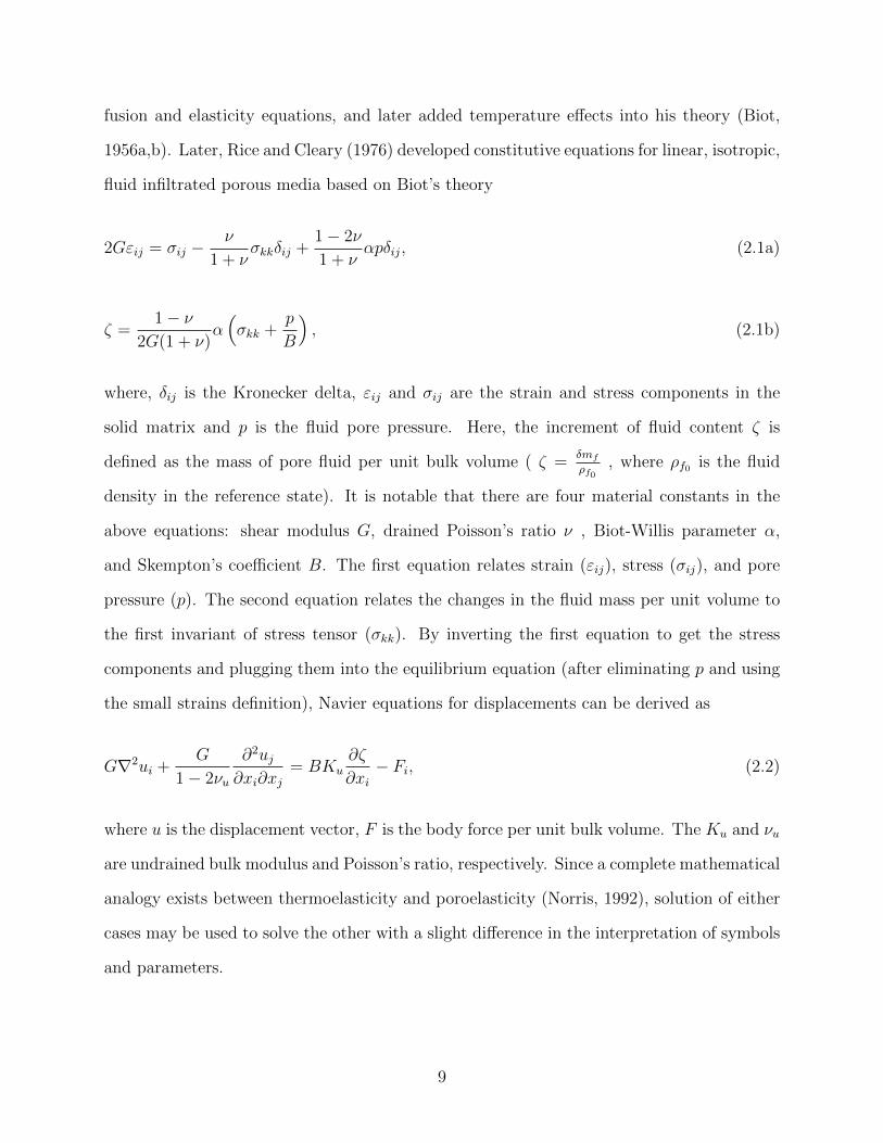
1956a,b). Later, Rice and Cleary (1976) developed constitutive equations for linear, isotropic,

fluid infiltrated porous media based on Biot’s theory

2Gεij = σij −ν

1 + νσkkδij +

1− 2ν

1 + ναpδij, (2.1a)

ζ =1− ν

2G(1 + ν)α(σkk +

p

B

), (2.1b)

where, δij is the Kronecker delta, εij and σij are the strain and stress components in the

solid matrix and p is the fluid pore pressure. Here, the increment of fluid content ζ is

defined as the mass of pore fluid per unit bulk volume ( ζ =δmf

ρf0, where ρf0 is the fluid

density in the reference state). It is notable that there are four material constants in the

above equations: shear modulus G, drained Poisson’s ratio ν , Biot-Willis parameter α,

and Skempton’s coefficient B. The first equation relates strain (εij), stress (σij), and pore

pressure (p). The second equation relates the changes in the fluid mass per unit volume to

the first invariant of stress tensor (σkk). By inverting the first equation to get the stress

components and plugging them into the equilibrium equation (after eliminating p and using

the small strains definition), Navier equations for displacements can be derived as

G∇2ui +G

1− 2νu

∂2uj∂xi∂xj

= BKu∂ζ

∂xi− Fi, (2.2)

where u is the displacement vector, F is the body force per unit bulk volume. The Ku and νu

are undrained bulk modulus and Poisson’s ratio, respectively. Since a complete mathematical

analogy exists between thermoelasticity and poroelasticity (Norris, 1992), solution of either

cases may be used to solve the other with a slight difference in the interpretation of symbols

and parameters.

9

Considering the small size of hydrocarbon reservoirs in comparison to the geological struc-

tures, one may consider reservoirs as inclusions embedded inside an infinite medium. This

assumption is made because reservoirs’ pore pressures may change due to production, and

they may not have similar lithology as the surrounding rocks. Reservoir subsidence, wellbore

stability, closure of natural fractures and seismic activities near the faults are some of the

negative consequences of the changes in stress and pore pressures in reservoirs. Each of

these issues may affect hydrocarbon production in a different way. Rudnicki (2002) modified

Eshelby‘s method to calculate stresses in poroelastic inclusions with different pore pressures,

temperatures or elastic moduli. Soltanzadeh et al. (2007) used Eshelby‘s method to provide

effective stress analysis for reservoir compaction due to hydrocarbon production, and found

stress changes induced by a uniform pressure change in an ellipsoidal reservoir embedded in

an infinite medium. Chen (2011) solved this problem for a single ellipsoidal poroelastic or

thermoelastic inclusion embedded in an infinite elastic body. He also considered double in-

clusion problem, using Hori and Nemat-Nasser (1993) method, in the case that one inclusion

encompasses the other one.

In the present work, the stress distribution in the presence of interacting poroelastic

inhomogeneities is studied. To have a better understanding of the presented solution, we

first briefly review Eshelby‘s problem in elasticity, and then we will go through required

modifications of this formula for poroelasticity. Problems involving interacting inclusions are

mostly studied using superposition of elastic fields. Moschovidis and Mura (1975) studied two

ellipsoidal non-intersecting inclusions by approximating equivalent eigenstrain using Taylor‘s

series expansions of Eshelby‘s tensors. Solutions derived using this method is confirmed

by numerical finite element calculations (Fond et al., 2001). Shodja et al. (2003) revised

this method to achieve a more computationally efficient one by eliminating unnecessary

evaluation of derivatives of Eshelby‘s tensors. Here, we extend the poroelastic solution for

a single inclusion to two interacting inclusions. The methodology used in this paper is a

10

00

11

Figure 2.1: A single inclusion embedded in an infinite medium. Ω1 and C1 are indicatinginclusion domain and its elastic moduli tensor, respectively. Ω0 and C0 are representing thesurrounding matrix and its elasticity moduli tensor, respectively.

combination of previous results for poroelastic inclusions and Moschovidis and Mura (1975)

approach to solve for interactions between poroelastic inclusions.

2.2 Single Inclusion

2.2.1 Elastic inclusions

The problem of an embedded ellipsoidal inclusion (C0ijkl = C1

ijkl = Cijkl)3 in an infinite

elastic medium, which undergoes a uniform inelastic deformation has been solved by Es-

helby (Eshelby, 1957). The contact boundary condition between inclusion and matrix is a

welded contact i.e., there is no slippage on the boundary. Figure 3.1 shows a schematic view

of the Eshelby’s problem. For the case of homogenous ellipsoidal inclusions with uniform

eigenstrain, ε∗, Eshelby (1957) solved the stress and displacement fields for both inside and

outside of the inclusion through defining a tensor, Sijkl or so-called Eshelby’s tensor. Es-

helby’s tensor is a forth rank tensor, and in the case of single inclusion problems is a function

of geometry and Poisson’s ratio of the inclusion (see Mura (1987) for more details about the

components of tensor S and its derivation). The main result of the Eshelby’s solution can

3For isotropic materials, elastic moduli is given byCijkl = 2Gν

1−2ν δijδkl +G(δikδjl + δilδjk) .

11

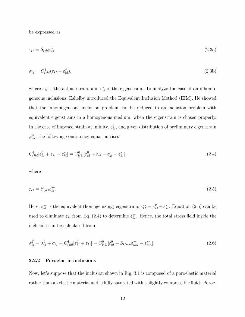
be expressed as

εij = Sijklε∗kl, (2.3a)

σij = C1ijkl(εkl − ε∗kl), (2.3b)

where εij is the actual strain, and ε∗kl is the eigenstrain. To analyze the case of an inhomo-

geneous inclusions, Eshelby introduced the Equivalent Inclusion Method (EIM). He showed

that the inhomogeneous inclusion problem can be reduced to an inclusion problem with

equivalent eigenstrains in a homogenous medium, when the eigenstrain is chosen properly.

In the case of imposed strain at infinity, ε0kl, and given distribution of preliminary eigenstrain

,εpkl, the following consistency equation rises

C1ijkl[ε

0kl + εkl − εpkl] = C0

ijkl[ε0kl + εkl − εpkl − ε

∗kl], (2.4)

where

εkl = Sijklε∗∗kl . (2.5)

Here, ε∗∗kl is the equivalent (homogenizing) eigenstrain, ε∗∗kl = εpkl + ε∗kl. Equation (2.5) can be

used to eliminate εkl from Eq. (2.4) to determine ε∗∗kl . Hence, the total stress field inside the

inclusion can be calculated from

σTij = σ0ij + σij = C1

ijkl[ε0kl + εkl] = C0

ijkl[ε0kl + Sklmnε

∗∗mn − ε∗∗mn]. (2.6)

2.2.2 Poroelastic inclusions

Now, let’s suppose that the inclusion shown in Fig. 3.1 is composed of a poroelastic material

rather than an elastic material and is fully saturated with a slightly compressible fluid. Poroe-

12

lastic inclusions may have different elastic or poroelastic properties, and even have different

fluid pressure from the surrounding medium. We further assume that there is no hydraulic

communication between the inclusion and the surrounding medium; therefore, the fluid pres-

sure in the surrounding rock will not change due to fluid pressure changes in the inclusion.

Hence, the surrounding medium may deform in drained conditions. These assumptions are

reasonable for modeling situations like rock compaction-drive and gas expansion-drive hy-

drocarbon reservoirs, or geological carbon sequestration (Rudnicki, 2011; Soltanzadeh and

Hawkes, 2012). The lack of hydraulic communication could be provided by a cap rock or

faults limiting the formation. For example, high permeability sandstone formations could

be contained by extremely low permeability shale layers.

Despite the popularity of Eshelby’s equivalent inclusion method in elasticity, this method

has not been fully developed for poroelasticity problems except for a few limited cases.

Rudnicki (2002) used the Eshelby’s equivalent inclusion method to calculate the alteration

of local stresses induced by a single inclusion with elastic moduli and pore pressure different

from those of the surrounding medium. Using basic linear poroelasticity principles, stress

inside the inhomogeneity can be written as (Rice and Cleary, 1976)

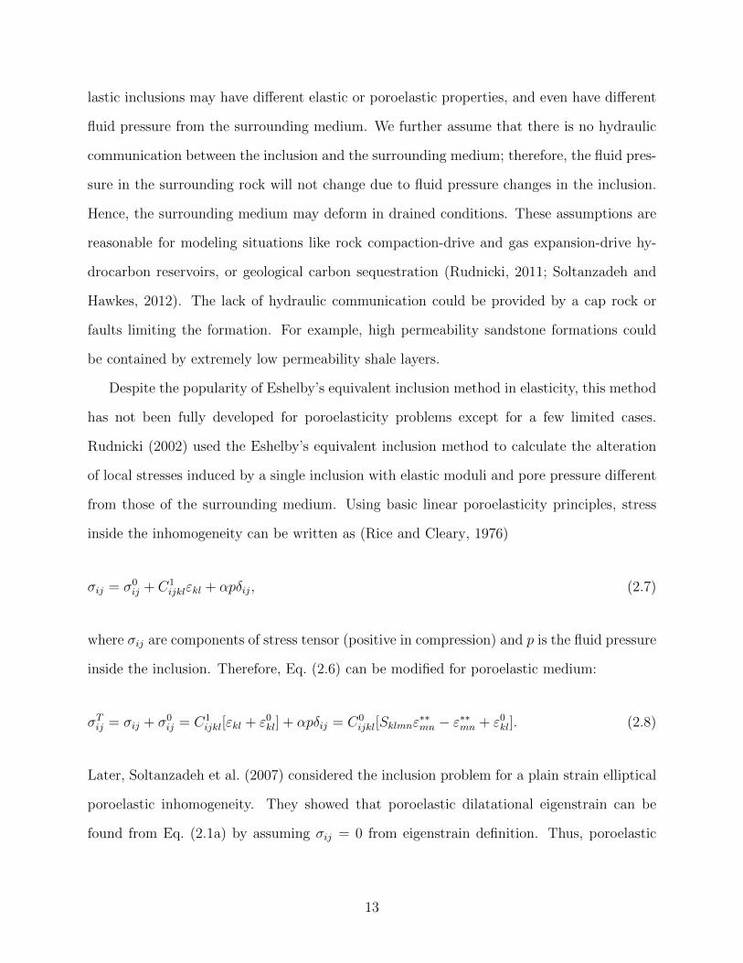
σij = σ0ij + C1

ijklεkl + αpδij, (2.7)

where σij are components of stress tensor (positive in compression) and p is the fluid pressure

inside the inclusion. Therefore, Eq. (2.6) can be modified for poroelastic medium:

σTij = σij + σ0ij = C1

ijkl[εkl + ε0kl] + αpδij = C0

ijkl[Sklmnε∗∗mn − ε∗∗mn + ε0

kl]. (2.8)

Later, Soltanzadeh et al. (2007) considered the inclusion problem for a plain strain elliptical

poroelastic inhomogeneity. They showed that poroelastic dilatational eigenstrain can be

found from Eq. (2.1a) by assuming σij = 0 from eigenstrain definition. Thus, poroelastic

13

eigenstrain can be expressed as

ε∗ij =α(1− 2ν)

2G(1 + ν)pδij. (2.9)

All previous methods result in uniform stress and strain distribution inside the inclusion,

when the medium is subjected to constant far-field stress and the fluid pressure is constant.

However, in the double inclusion case, due to interaction of the inhomogeneities, the stress

and strain fields inside the inclusions are no longer uniform, which was the main motivation

for studying interacting double poroelastic inclusions problem.

2.3 Two Inclusions

In most practical cases, inclusions are generally existing in large quantities. Existence of

multiple inclusions and their interactions affect the stress field in the medium. For instance,

uniform stress and strain inside the inclusion is no longer valid for multiple inclusions problem

(Shodja and Sarvestani, 2001). An easy approach to deal with this problem is superposing

elastic solutions for single inclusions; or in other words, ignoring the interaction between

inclusions (Nemat-Nasser and Hori, 1999). Although this method could be a good approx-

imation when inclusions are located far enough from each other, their interactions may not

be ignored when they are closely located.

In this section, we derive the stress field of two interacting poroelastic inclusions by

modifying Moschovidis and Mura (1975) solution for two interacting elastic inclusions.

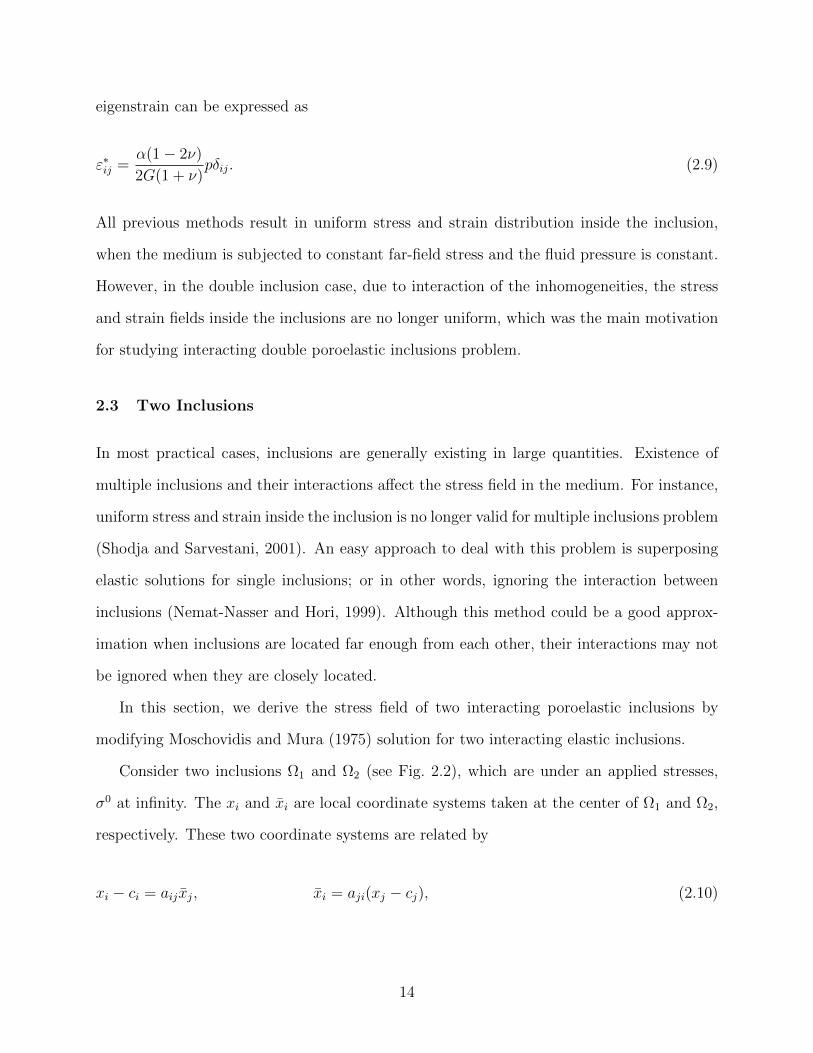
Consider two inclusions Ω1 and Ω2 (see Fig. 2.2), which are under an applied stresses,

σ0 at infinity. The xi and xi are local coordinate systems taken at the center of Ω1 and Ω2,

respectively. These two coordinate systems are related by

xi − ci = aijxj, xi = aji(xj − cj), (2.10)

14

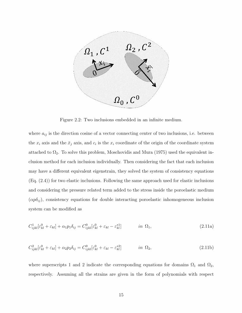
Figure 2.2: Two inclusions embedded in an infinite medium.

where aij is the direction cosine of a vector connecting center of two inclusions, i.e. between

the xi axis and the xj axis, and ci is the xi coordinate of the origin of the coordinate system

attached to Ω2. To solve this problem, Moschovidis and Mura (1975) used the equivalent in-

clusion method for each inclusion individually. Then considering the fact that each inclusion

may have a different equivalent eigenstrain, they solved the system of consistency equations

(Eq. (2.4)) for two elastic inclusions. Following the same approach used for elastic inclusions

and considering the pressure related term added to the stress inside the poroelastic medium

(αpδij), consistency equations for double interacting poroelastic inhomogeneous inclusion

system can be modified as

C1ijkl[ε

0kl + εkl] + α1p1δij = C0

ijkl[ε0kl + εkl − ε∗1kl ] in Ω1, (2.11a)

C2ijkl[ε

0kl + εkl] + α2p2δij = C0

ijkl[ε0kl + εkl − ε∗2kl ] in Ω2, (2.11b)

where superscripts 1 and 2 indicate the corresponding equations for domains Ω1 and Ω2,

respectively. Assuming all the strains are given in the form of polynomials with respect

15

to the local Cartesian coordinate system (see Section 2.6), the applied strain before the

disturbance (ε0ij(x) and ε0

ij(x)) can be written as

ε0ij(x) = Eij + Eijkxk + Eijklxkxl + · · · , (2.12a)

ε0ij(x) = Eij + Eijkxk + Eijklxkxl + · · · . (2.12b)

Here, Eij... are constants and the variables with a bar are defined with respect to second

inclusion coordination system. Analogously, equivalent eigenstrains (ε∗1ij (x) and ε∗2ij (x)) can

be defined as

ε∗1ij (x) = B1ij +B1

ijkxk +B1ijklxkxl + · · · , (2.13a)

ε∗2ij (x) = B2ij +B2

ijkxk +B2ijklxkxl + · · · , (2.13b)

where Bij... are constants. Using the concept of higher ranked Eshelby’s tensors (see Sec-

tion 2.6) and Eq. (2.3a), the strains associated with the eigenstrains will be equal to

ε1ij(x) = D1

ijkl(x)B1kl +D1

ijklq(x)B1klq +D1

ijklqr(x)B1klqr + · · · , (2.14a)

ε2ij(x) = D2

ijkl(x)B2kl +D2

ijklq(x)B2klq +D2

ijklqr(x)B2klqr + · · · . (2.14b)

In the above equations, D represents higher order Eshelby’s tensors. For x in Ω1, D1(x)

are polynomials of x in Ω1, and D2(x) are expanded by Taylor series around the origin of

the associated local coordinate system. Whereas, for x in Ω2, D2(x) are polynomials of x in

Ω2, and D1(x) are approximated by a Taylor expansion of x in Ω2. Then the strain, εkl, in

16

Eq. (2.11) is the sum of ε1ij(x) and ε2

ij(x)

εij(x) = ε1ij(x) + ε2

ij(x). (2.15)

Using Eqs. (2.12) and (2.14) in the system of Eq. (2.11), values for B1 and B2 can be

obtained. Finally, it is sufficient to solve the consistency equations in Ω1 and Ω2, to find the

constants of polynomial parts of eigenstrain, B. Consequently in Ω1 we will have

∆C1stmn

[D1mnij(0)B1

ij +D1mnijkl(0)B1

ijkl + · · ·]

+ amcanh

[D2chij(0)B2

ij +D2chijk(0)B2

ijk +D2chijkl(0)B2

ijkl + · · ·]

− C0stmnB

1mn = −∆C1

stmnEmn − α1p1δst,

∆C1stmn

[ ∂

∂xpD1mnijk(0)B1

ijk + · · ·]

+ amcanhapf

[ ∂

∂xfD2chij(0)B2

ij +∂

∂xfD2chijk(0)B2

ijk +∂

∂xfD2chijkl(0)B2

ijkl + · · ·]

− C0stmnB

1mnp = −∆C1

stmnEmnp,

etc.

(2.16)

To solve the above system of equations, the coefficients of the power series in the left and

right hand sides of the equations should be equated. Similar system of equations should be

solved for the second inclusion, Ω2

∆C2stmn

[D2mnij(0)B2

ij +D2mnijkl(0)B2

ijkl + · · ·]

+ acmahn

[D1chij(0)B1

ij +D1chijk(0)B1

ijk +D1chijkl(0)B1

ijkl + · · ·]

− C0stmnB

2mn = −∆C2

stmnEmn − α2p2δst,

17

∆C2stmn

[ ∂

∂xpD2mnijk(0)B2

ijk + · · ·]

+ acmahnafp

[ ∂

∂xfD1chij(0)B1

ij +∂

∂xfD1chijk(0)B1

ijk +∂

∂xfD1chijkl(0)B1

ijkl + · · ·]

− C0stmnB

2mnp = −∆C2

stmnEmnp,

etc.

(2.17)

Here, ∆Cistmn = C0

stmn − Cistmn, i = 1, 2 and Bij... are the coefficients of the polynomial

expansion of poroelastic eigenstrains. By obtaining B1 and B2, final strains can be calculated

by Eqs. (2.14) and (2.15). The accuracy of results depends on the degree of polynomials

employed; however, the dependency is only substantial for very strong interaction effects.

2.4 Results and Discussions

We start this section with two verification examples for solutions developed in previous

sections. Let’s consider two ellipsoidal inhomogeneities embedded in an infinite poroelastic

medium with applied stresses σ0ij at infinity. For simplification purposes, the principal axes

of the inhomogeneities (i.e. xi and xi axes) are assumed to be aligned with the Cartesian

coordinate system. Figure 2.3 shows the configuration of the inhomogeneities, in which

∆i is the distance between centers of the inhomogeneities along the i − th coordinate axis

(i = 1, 2, 3). The dimension of ellipsoidal inclusions along the corresponding coordinate axes

are denoted by ai and ai, respectively (i = 1, 2, 3). To verify the accuracy of the proposed

approach, we first consider the special case in which fluid pressure is kept constant. Hence,

the problem is simplified to two elastic inhomogeneities, which are previously solved by

Moschovidis and Mura (1975). Figures 2.4(b) and 2.5(b) demonstrates the σ33-stress along

the x3 and x1 axes (shown in Fig. 2.3) for inclusions under uniform tensile loading at infinity

(σ033 = 1) and different shear modulus ratios of inclusion and matrix, γ. These results are

verified to be in exact agreement with the results obtained by Moschovidis and Mura (1975),

18

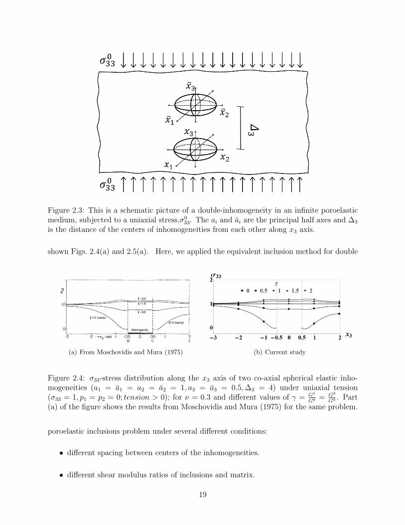
Figure 2.3: This is a schematic picture of a double-inhomogeneity in an infinite poroelasticmedium, subjected to a uniaxial stress,σ0

33. The ai and ai are the principal half axes and ∆3

is the distance of the centers of inhomogeneities from each other along x3 axis.

shown Figs. 2.4(a) and 2.5(a). Here, we applied the equivalent inclusion method for double

(a) From Moschovidis and Mura (1975) (b) Current study

Figure 2.4: σ33-stress distribution along the x3 axis of two co-axial spherical elastic inho-mogeneities (a1 = a1 = a2 = a2 = 1, a3 = a3 = 0.5,∆3 = 4) under uniaxial tension(σ33 = 1, p1 = p2 = 0; tension > 0); for ν = 0.3 and different values of γ = G1

G0 = G2

G0 . Part(a) of the figure shows the results from Moschovidis and Mura (1975) for the same problem.

poroelastic inclusions problem under several different conditions:

• different spacing between centers of the inhomogeneities.

• different shear modulus ratios of inclusions and matrix.

19

(a) From Moschovidis and Mura (1975) (b) Current study

Figure 2.5: The above graphs show σ33-stress along the x1 axis of two co-axial sphericalelastic inhomogeneities (a1 = a1 = a2 = a2 = 1, a3 = a3 = 0.5,∆3 = 4) in uniaxial tension(σ33 = 1, p1 = p2 = 0; tension > 0); for ν = 0.3 and different values of γ = G1

G0 = G2

G0 . Part(a) of the figure shows the results from Moschovidis and Mura (1975) for the same problem.

• different size of the inclusions.

• different pressure value inside the inclusions.

Due to the primary interest of the authors in subsurface problems, compressive stresses are

assumed to be positive, hereafter. Figure 2.6 shows the effect of distance between centers of

the two co-axial spherical poroelastic inhomogeneities and demonstrates how stress regime

changes when inclusions laying closer to each other. As inclusions become closer to each

other, they start interacting with each other, so stresses inside the inclusions become non-

uniform, especially in stiffer inclusions. Comparison of Figs. 2.4 and 2.6(a) shows more

compressive normal stresses near the pressurized inclusions as opposed to elastic inclusions,

especially in inclusions with elastic moduli lower than that of the medium. This trend

agrees with observations in depleted formations (Sayers et al., 2007). For example, lower

mud weights should be used to drill depleted formations to avoid lost circulation; or hydraulic

fracture jobs can be done more effective after depletion of a reservoir (Zoback, 2007). As a

reservoir depletes due to production, the total horizontal stress in the reservoir rock decreases.

20

Consequently, fracture gradient decreases inside the reservoir as reservoir tends to shrink

but confined by surrounding rocks. Reservoir shrinkage causes the horizontal stresses to

redistribute and become more compressive above and below the reservoir (Segall, 1989).

These changes in the stress field may cause faulting or seismic activities inside and outside

of the reservoir.

Here, we assumed that depletion or pore pressure variations in the reservoir will not

change the pore pressure in the surrounding rocks as low permeability cap rock hinders any

hydraulic communication between the reservoir and the surrounding rocks. It is notable that

since the size of reservoirs are assumed to be much less than the surrounding rocks, hence

pore pressure in the surrounding rocks is mainly a hydrostatic pressure. Therefore, we may

consider the surrounding rock in the effective stress mode or simply as an elastic medium.

In Fig. 2.7, we showed how the size of inclusions affects the stress distribution around

the inclusion. Figures 2.7(a) and 2.7(c) show that normal compressive stresses will be higher

in larger inclusions with greater shear modulus ratio, γ. Furthermore for stiff inclusions,

compressive stresses near the larger inclusion is greater than that of the smaller one. However,

for softer inclusions, the minimum compressive stress in the medium occurs in the vicinity

of the larger inclusion.

Finally, Fig. 2.8 shows stress distribution around inclusions with different pore pressures

and different sizes. It can be seen that for an unequal pressurized double inclusion system,

compressive stresses inside the softer inclusion is larger than that of the stiffer inclusion.

Considering Figs. 2.6 to 2.8, the distance between the inclusions, elasticity modulus ratio,

initial stresses and pore pressure conditions are the major factors that may affect the final

stress distribution around two inclusions.

2.5 Summary

In this article, an analytical approach originally developed by Moschovidis and Mura (1975)

for determining stress distribution around two interacting elastic inhomogeneities, was adopted

21

(a) σ33 along x3, ∆3 = 4, p1 = p2 = 1 (b) σ11 along x3, ∆3 = 4, p1 = p2 = 1

(c) σ33 along x3, ∆3 = 3, p1 = p2 = 1 (d) σ11 along x3, ∆3 = 3, p1 = p2 = 1

(e) σ33 along x3, ∆3 = 2, p1 = p2 = 1 (f) σ11 along x3, ∆3 = 2, p1 = p2 = 1

Figure 2.6: The above graphs show the effect of spacing between two co-axial sphericalporoelastic inhomogeneities, ∆3, on σ33 and σ11-stresses along the x3 axis; (a1 = a1 = a2 =a2 = 1, a3 = a3 = 0.5). Inclusions are uniformly pressurized and under uniaxial compression(σ33 = 1, p1 = p2 = 1;Compression > 0). The plots are generated for ν = 0.3 and differentvalues of γ = G1

G0 = G2

G0 .

for double poroelastic interacting inhomogeneous inclusions. These inclusions are assumed

to be embedded in an infinite elastic medium and under nonuniform far-field loading. This

method is applicable to three-dimensional problems, and inclusions may be oriented ar-

bitrarily with respect to each other. Using the Equivalent Inclusion Method (EIM) and

polynomial expansion of strain fields in the local coordinate systems, we solved for two ellip-

22

(a) σ33 along x3, ∆3 = 4, p1 = p2 = 1 (b) σ11 along x3, ∆3 = 4, p1 = p2 = 1

(c) σ33 along x3, ∆3 = 3, p1 = p2 = 1 (d) σ11 along x3, ∆3 = 3, p1 = p2 = 1

Figure 2.7: The above graphs show the effect of size of the two co-axial spherical poroelasticinhomogeneities on σ33 and σ11-stresses along the x3 axis; (a1 = a1 = a2 = a2 = 1, a3 =0.5, a3 = 1). Inclusions are uniformly pressurized and under uniaxial compression (σ33 =1, p1 = p2 = 1;Compression > 0). The plots are generated for ν = 0.3 and different valuesof γ = G1

G0 = G2

G0 .

soidal poroelastic inhomogeneities. To solve this problem eigenstrains were expanded, and

higher order Eshelby’s tensors and their derivatives were calculated at the center of each

inhomogeneity. To get more accurate results, it is necessary to use more polynomial terms

for eigenstrains and higher rank Eshelby’s tensors, especially when dealing with very close

inclusions. The results show that the distance of centers of the inhomogeneities and their

relative stiffness to the medium affect the associated stress field. Considering same distance

for inhomogeneities, the interaction effect is more significant on stiffer inclusions. Poroelastic

inclusions could have a wide range of applications from rock mechanics problems to tissue

mechanics. Here, we utilized this solution to investigate earth stress changes around depleted

hydrocarbon reservoirs.

23

(a) σ33 along x3, ∆3 = 4, p1 = 1, p2 = 2 (b) σ11 along x3, ∆3 = 4, p1 = 1, p2 = 2

(c) σ33 along x3, ∆3 = 3, p1 = 1, p2 = 2 (d) σ11 along x3, ∆3 = 3, p1 = 1, p2 = 2

Figure 2.8: The above graphs show the effect of different pressure values inside the thetwo co-axial spherical poroelastic inhomogeneities on σ33 and σ11-stresses along the x3 axis;(a1 = a1 = a2 = a2 = 1, a3 = a3 = 0.5). Inclusions are uniformly pressurized and underuniaxial compression (σ33 = 1, p1 = 1, p2 = 2;Compression > 0). The plots are generatedfor ν = 0.3 and different values of γ = G1

G0 = G2

G0 .

2.6 Polynomial Eigenstrains

The strain field can be expressed by a polynomial function of coordinates. Here, a short

derivation is presented. For Complete derivation and more details, the reader may check

Sendeckyj (1967), Moschovidis (1975), Moschovidis and Mura (1975), and Mura (1987).

Eshelby (1957), showed that the elastic field in the existence of an inclusion can be written

as

ui(x) = −∫

Ω

Cjkmnε∗mn(x′)Gij,k(x− x′) dx′, (2.18)

24

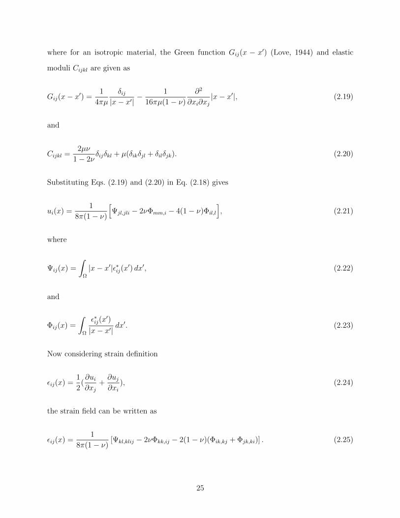
where for an isotropic material, the Green function Gij(x − x′) (Love, 1944) and elastic

moduli Cijkl are given as

Gij(x− x′) =1

4πµ

δij|x− x′|

− 1

16πµ(1− ν)

∂2

∂xi∂xj|x− x′|, (2.19)

and

Cijkl =2µν

1− 2νδijδkl + µ(δikδjl + δilδjk). (2.20)

Substituting Eqs. (2.19) and (2.20) in Eq. (2.18) gives

ui(x) =1

8π(1− ν)

[Ψjl,jli − 2νΦmm,i − 4(1− ν)Φil,l

], (2.21)

where

Ψij(x) =

∫Ω

|x− x′|ε∗ij(x′) dx′, (2.22)

and

Φij(x) =

∫Ω

ε∗ij(x′)

|x− x′|dx′. (2.23)

Now considering strain definition

εij(x) =1

2(∂ui∂xj

+∂uj∂xi

), (2.24)

the strain field can be written as

εij(x) =1

8π(1− ν)[Ψkl,klij − 2νΦkk,ij − 2(1− ν)(Φik,kj + Φjk,ki)] . (2.25)

25

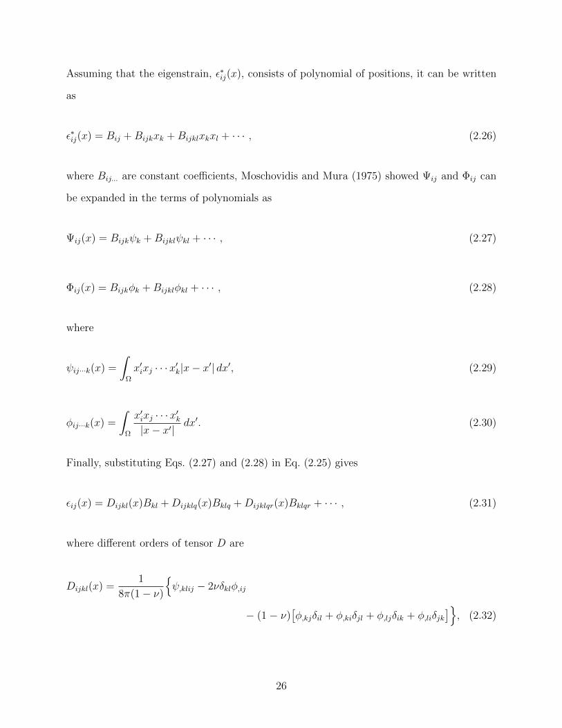
Assuming that the eigenstrain, ε∗ij(x), consists of polynomial of positions, it can be written

as

ε∗ij(x) = Bij +Bijkxk +Bijklxkxl + · · · , (2.26)

where Bij... are constant coefficients, Moschovidis and Mura (1975) showed Ψij and Φij can

be expanded in the terms of polynomials as

Ψij(x) = Bijkψk +Bijklψkl + · · · , (2.27)

Φij(x) = Bijkφk +Bijklφkl + · · · , (2.28)

where

ψij···k(x) =

∫Ω

x′ixj · · ·x′k|x− x′| dx′, (2.29)

φij···k(x) =

∫Ω

x′ixj · · ·x′k|x− x′|

dx′. (2.30)

Finally, substituting Eqs. (2.27) and (2.28) in Eq. (2.25) gives

εij(x) = Dijkl(x)Bkl +Dijklq(x)Bklq +Dijklqr(x)Bklqr + · · · , (2.31)

where different orders of tensor D are

Dijkl(x) =1

8π(1− ν)

ψ,klij − 2νδklφ,ij

− (1 − ν)[φ,kjδil + φ,kiδjl + φ,ljδik + φ,liδjk

], (2.32)

26

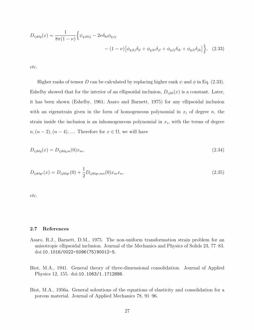
Dijklq(x) =1

8π(1− ν)

ψq,klij − 2νδklφq,ij

− (1 − ν)[φq,kjδil + φq,kiδjl + φq,ljδik + φq,liδjk

], (2.33)

etc.

Higher ranks of tensor D can be calculated by replacing higher rank ψ and φ in Eq. (2.33).

Eshelby showed that for the interior of an ellipsoidal inclusion, Dijkl(x) is a constant. Later,

it has been shown (Eshelby, 1961; Asaro and Barnett, 1975) for any ellipsoidal inclusion

with an eigenstrain given in the form of homogeneous polynomial in xi of degree n, the

strain inside the inclusion is an inhomogeneous polynomial in xi, with the terms of degree

n, (n− 2), (n− 4), .... Therefore for x ∈ Ω, we will have

Dijklq(x) = Dijklq,m(0)xm, (2.34)

Dijklqr(x) = Dijklqr(0) +1

2Dijklqr,mn(0)xmxn, (2.35)

etc.

2.7 References

Asaro, R.J., Barnett, D.M., 1975. The non-uniform transformation strain problem for ananisotropic ellipsoidal inclusion. Journal of the Mechanics and Physics of Solids 23, 77–83.doi:10.1016/0022-5096(75)90012-5.

Biot, M.A., 1941. General theory of three-dimensional consolidation. Journal of AppliedPhysics 12, 155. doi:10.1063/1.1712886.

Biot, M.A., 1956a. General soloutions of the equations of elasticity and consolidation for aporous material. Journal of Applied Mechanics 78, 91–96.

27

Biot, M.A., 1956b. Theory of deformation of a porous viscoelastic anisotropic solid. Journalof Applied Physics 27, 459. doi:10.1063/1.1722402.

Chen, Z.R., 2011. Poroelastic model for induced stresses and deformations in hydrocar-bon and geothermal reservoirs. Journal of Petroleum Science and Engineering 80, 41–52.doi:10.1016/j.petrol.2011.10.004.

Eshelby, J.D., 1957. The determination of the elastic field of an ellipsoidal inclusion, andrelated problems. Proceedings of the Royal Society A: Mathematical, Physical and Engi-neering Sciences 241, 376–396. doi:10.1098/rspa.1957.0133.

Eshelby, J.D., 1959. The elastic field outside an ellipsoidal inclusion, in: Proceedings of theRoyal Society of London. Series A, Mathematical and Physical, pp. 561–569.

Eshelby, J.D., 1961. Elastic inclusions and inhomogeneities, in: Sneddon, I.N., Hill, R.(Eds.), Progress in Solid Mechanics, Vol.2. North-Holland, Amsterdam, pp. 89–140.

Fond, C., Riccardi, A., Schirrer, R., Montheillet, F., 2001. Mechanical interaction betweenspherical inhomogeneities: an assessment of a method based on the equivalent inclu-sion. European Journal of Mechanics - A/Solids 20, 59–75. doi:10.1016/S0997-7538(00)01118-9.

Hori, M., Nemat-Nasser, S., 1993. Double-inclusion model and overall moduli of multi-phasecomposites. Mechanics of Materials 14, 189–206. doi:10.1016/0167-6636(93)90066-Z.

Love, A.E.H., 1944. A treatise on the mathematical theory of elasticity. Dover Publications,New York.

Marquez, J.P., Genin, G.M., Zahalak, G.I., Elson, E.L., 2005. Thin bio-artificial tissues inplane stress: the relationship between cell and tissue strain, and an improved constitutivemodel. Biophysical journal 88, 765–77. doi:10.1529/biophysj.104.040808.

Moschovidis, Z.A., 1975. Two ellipsoidal inhomogeneities and related problems treated bythe equivalent inclusion method. Ph.D. thesis. Northwestern University, Evanston.

Moschovidis, Z.A., Mura, T., 1975. Two-ellipsoidal inhomogeneities by the Equivalent In-clusion Method. Journal of Applied Mechanics 42, 847. doi:10.1115/1.3423718.

28

Mura, T., 1987. Micromechanics of defects in solids. Martinus Nijhoff Publishers.

Nemat-Nasser, S., Hori, M., 1999. Micromechanics: overall properties of heterogeneousmaterials. Elsevier, Amsterdam.

Norris, A., 1992. On the correspondence between poroelasticity and thermoelasticity. Journalof Applied Physics 71, 1138. doi:10.1063/1.351278.

Rice, J.R., Cleary, M.P., 1976. Some basic stress diffusion solutions for fluid-saturatedelastic porous media with compressible constituents. Reviews of Geophysics 14, 227.doi:10.1029/RG014i002p00227.

Richard M. Christensen, 2012. Mechanics of composite materials. Courier Dover Publica-tions.

Rudnicki, J.W., 2002. Alteration of regional stress by reservoirs and other inhomo- geneities:Stabilizing or destabilizing?, in: Vouille, G., Berest, P. (Eds.), Proc. 9th Int. Congr. RockMechanics,Vol. 3, Paris, Aug. 25-29, 1999, Paris, France. pp. 1629– 1637.

Rudnicki, J.W., 2011. Eshelbys technique for analyzing inhomogeneities in geomechanics,in: Leroy, Y.M., Lehner, F.K. (Eds.), Mechanics of Crustal Rocks. Springer Vienna, pp.43–72. doi:10.1007/978-3-7091-0939-7.

Sayers, C., Kisra, S., Tagbor, K., Adachi, J.I., Dahi Taleghani, A., 2007. Calibrating themechanical properties and in-situ stresses using acoustic radial profiles, in: Proceedingsof SPE Annual Technical Conference and Exhibition, Society of Petroleum Engineers. pp.1–8. doi:10.2118/110089-MS.

Segall, P., 1989. Earthquakes triggered by fluid extraction. Geology 17, 942–946. doi:10.1130/0091-7613(1989)017\%3C0942:ETBFE\%3E2.3.CO;2BFE>2.3.CO;2.

Sendeckyj, G., 1967. Ellipsoidal inhomogeneity problem. Ph.D. thesis. North Western Uni-versity, Evanston.

Shodja, H.M., Rad, I., Soheilifard, R., 2003. Interacting cracks and ellipsoidal inhomo-geneities by the equivalent inclusion method. Journal of the Mechanics and Physics ofSolids 51, 945–960. doi:10.1016/S0022-5096(02)00106-0.

29

Shodja, H.M., Sarvestani, a.S., 2001. Elastic fields in double inhomogeneity by the EquivalentInclusion Method. Journal of Applied Mechanics 68, 3. doi:10.1115/1.1346680.

Soltanzadeh, H., Hawkes, C.D., 2012. Evaluation of caprock integrity during pore pressurechange using a probabilistic implementation of a closed-form poroelastic model. Interna-tional Journal of Greenhouse Gas Control 7, 30–38. doi:10.1016/j.ijggc.2011.10.006.

Soltanzadeh, H., Hawkes, C.D., Sharma, J.S., 2007. poroelastic model for production-and injection-induced stresses in reservoirs with elastic properties different from the sur-rounding rock. International Journal of Geomechanics 7, 353–361. doi:10.1061/(ASCE)1532-3641(2007)7:5(353).

Van der Molen, I., Van Roermund, H., 1986. The pressure path of solid inclusionsin minerals: the retention of coesite inclusions during uplift. Lithos 19, 317–324.doi:10.1016/0024-4937(86)90030-7.

Voyiadjis, G.Z., Kattan, P.I., 2006. Advances in damage mechanics: metals and metal matrixcomposites with an introduction to fabric tensors, 2nd Edition, in: Advances in DamageMechanics: Metals and Metal Matrix Composites With an Introduction to Fabric Tensors,2nd Edition. second edi ed.. Elsevier Science Ltd, Oxford, p. 740.

Zhou, K., Hoh, H.J., Wang, X., Keer, L.M., Pang, J.H., Song, B., Wang, Q.J., 2013. Areview of recent works on inclusions. Mechanics of Materials 60, 144–158. doi:10.1016/j.mechmat.2013.01.005.

Zoback, M.D., 2007. Reservoir geomechanics. Cambridge University Press, New York.

30

Chapter 3On the Inhomogeneous Anisotropic Poroe-lastic Inclusions

Anisotropy in elastic properties has been studied extensively in the last century; however,

anisotropy in poroelastic properties, despite its potential importance in different engineer-

ing problems, has not been explored thoroughly. In this paper, we provide the Eshelby

solution for stress and strain inside and outside of an anisotropic poroelastic inhomogeneity

due to pore pressure changes inside the inhomogeneity. Here, the term anisotropic inhomo-

geneity, refers to an inhomogeneity with anisotropic poroelastic constants. To tackle this

problem, we use the Equivalent Inclusion Method (EIM). Due to the authors’ primary in-

terest in geomechanical problems, discussions and examples are chosen for applications in

fluid withdrawal/injection into hydrocarbon reservoirs with transverse isotropic properties.

However, the results may have applications in other type of anisotropic poroelastic materials,

for instance biological tissues. These analytical results could be used a benchmark to exam-

ine different numerical solutions obtained by discretization of governing partial differential

equations.

3.1 Introduction

Inclusions are defined as finite sub-volumes of the medium, which may possess different strain

status from that of the surrounding environment. On the other hand, an inhomogeneity is a

sub-volume of a medium that has different material properties from those of its surrounding.

31

If the inhomogeneity experiences different loading status at the same time, it is considered as

inhomogeneous inclusion. Eshelby (1957, 1959, 1961) solved for stress distribution induced by

an ellipsoidal inhomogeneity embedded in an infinite isotropic elastic medium, that undergoes

a uniform strain. Later, Eshelby’s method has been used to solve more complex problems like

inclusions in finite media (Li et al., 2007), interacting inclusions (Shodja et al., 2003; Zhou

et al., 2012), or non-ellipsoidal inclusions (Zou et al., 2010). Eshelby’s solution has played

a vital role in development of many micromechanical models in mechanics of composites ,

fractures, dislocations, and phase transformations (Voyiadjis and Kattan, 2006; Shodja and

Ojaghnezhad, 2007; Li and Wang, 2008). Mura (1987) and Nemat-Nasser and Hori (1999) are

two references for more detailed information about the classic problems in the subject. For a

review of recent works on inclusions and inhomogeneities see Zhou et al. (2013). Application

of Eshelby solution is also recently extended to fluid saturated porous materials.

Presence of pore fluid in the elastic solid porous materials and its coupling with material

deformations leads to different class of material behaviors known as the theory of poroe-

lasticity. Poroelasticity assumed the continuum media are consisted of elastic solid matrix

and interconnected fluid saturated pores. Poroelastic materials present in a wide range of

applications in geomechanics and biomechanics (Berryman, 1997; Wang, 2000; Levin and

Alvarez-Tostado, 2003; Dormieux et al., 2006). Rocks, soils, biological tissues, bones, foams,

spongy metal alloys, and ceramics are few examples of poroelastic materials. Consider-

ing different material properties and different pressure/temperature of hydrocarbon bearing

formations in comparison to those of the surrounding geological structures, hydrocarbon

reservoirs can be considered as inhomogeneities embedded inside an infinite medium. Rud-

nicki (2002a,b); Soltanzadeh et al. (2007); Chen (2011); Soltanzadeh and Hawkes (2012);

Bedayat and Dahi Taleghani (2013, 2014) used the concept of poroelastic inhomogeneities

to model stress alterations in the subsurface due to pore fluid pressure changes. Similarly,

biological tissues and bones can also be modeled as poroelastic composites consisted of com-

plicated inhomogeneities. Eshelby theorem has been used widely in biomechanics to model

32

biomaterials disregarding poroelastic parameters of the medium (Ferrari, 2000; Hellmich and

Ulm, 2002; Marquez et al., 2005; Khoshgofta et al., 2007; Malekmotiei et al., 2013);

The theory of linear poroelasticity is originally developed to analyze geomechanical prob-

lems (Biot, 1941, 1955). Land subsidence, determination of stresses and displacements associ-

ated to fluid withdrawal or fluid injection (Teklu et al., 2012), or determining the rock in-situ

stresses (Wang et al., 2007), wellbore stability (Abousleiman and Ekbote, 2005; Mehrabian

and Abousleiman, 2013), carbon geological sequestration (Rutqvist et al., 2002), naturally

fractured reservoirs (Zhou and Ghassemi, 2011; Bedayat and Dahi Taleghani, 2012; Dahi

Taleghani et al., 2014), hydraulic fracturing (Detournay and Cheng, 1991), and geothermal

reservoirs (Rawal and Ghassemi, 2014). Meanwhile, the theory of linear poroelasticity is

used in biomechanics (Cederbaum et al., 2000) to model different organic materials ranging

from human skulls (Nowinski and Davis, 1970; Cowin, 1999) to soft tissues like cartilage

(Wu et al., 1999; Li et al., 2003).

Under undrained conditions that excessive pore pressure is not allowed to dissipate,

the mechanical response of porous solid-fluid system is dominated by two mechanisms: (i)

an increase of pore pressure causes dilation of the solid matrix, and (ii) as the solid part

compresses, pore pressure increases. However, under drained conditions, extra pore pressure

induced by compression of the solid phase dissipates and secondary deformation of the solid

phase takes place. These two mechanisms were formulated by Biot (Biot, 1941) through

coupling of fluid diffusion and elasticity equations (see Verruijt (2014) for the earlier history

and recent progresses in the theory of linear poroelasticity). Later on, Rice and Cleary (1976)

reformulated Biot’s constitutive equations for isotropic poroelastic materials as

εij =1

2G

[σij −

(3K − 2G

9K

)σkkδij +

2G

3Kαpδij

], (3.1)

ζα

K

(σkk3

+p

B

), (3.2)

33

where δij is the Kronecker delta (δij = 1 for i = j, and δij = 0 for i 6= j), εij and σij are the

components of strain and stress tensor in the solid matrix, respectively; and p is the pore

fluid pressure. The increment of fluid content, ζ, is defined as the mass of pore fluid δmf ,

per unit bulk volume

ζ =δmf

ρf0, (3.3)

where ρf0 is the pore fluid density in the reference state. There are four material constants

in the above equations (compared to two for isotropic elastic materials; B is the Skempton’s

coefficient).

The Biot coefficient, α, represents the influence of pore fluid pressure on the elastic solid

matrix and is a function of solid constituent properties or more specifically pore geometries.

The Biot coefficient for isotropic materials is defined as

α = 1− K

Ks

, (3.4)

where Ks is bulk modulus of the solid material. It can be shown that the range of variation

for Biot coefficient is φ < α < 1 (Berryman, 1992), where φ is the material porosity.

Similar to the elasticity, most fundamental studies of poroelastic materials assumes

isotropic conditions for the medium. The material properties are considered to be isotropic,

if their values at a certain point are the same in all directions. In biomechanics, most

organic tissues are anisotropic due to their microstructures. For example, bones consid-

ered to be anisotropic due to the lamella structure (Turner et al., 1995; Cowin and Doty,

2007). Similarly, anisotropic properties may occur in rocks due to the microstructure geome-

tries (Hudson, 1981; Ghabezloo and Hemmati, 2011; Levasseur et al., 2013; He et al., 2013;

Ahmadi et al., 2014a) of the material, sedimentologic layering of rock or damage induced

isotropy in an initially isotropic material (Litewka, 2003; Shao et al., 2006; Ahmadi et al.,

2014b). Rock anisotropy occurs in different scales ranging from grain-size scale to the large

34

scale rock masses would show its consequences in engineering problems like drilling vertical

or horizontal wells (Aadnoy, 1988).

Poroelastic anisotropy is also utilize to study material behavior in other type of materials

as well (Bruschke and Advani, 1990; Shao, 1998; Kanj et al., 2003; Berryman, 2011) too.

There are some studies on assessing the impact of anisotropy on fluid flow in geological struc-

tures that show neglecting the effect of rock anisotropy may cause unexpected and unrealistic

results in failure analysis of geomaterials (Cui et al., 1996; Cheng et al., 1996). Borehole

stability analysis (Aoki et al., 1993), effective medium theory in seismology (Schoenberg and

Sayers, 1995; Sayers, 2005), hydraulic fracturing (Dahi Taleghani and Olson, 2011; Khan

et al., 2012; Shojaei et al., 2014), formation evaluation (Moran and Gianzero, 1979; Bang

et al., 2001), and fluid flow in porous media (Rickman, 2009) are some other examples that

considering rock anisotropy would have a significant role on the reliability of engineering

analyses.

For a poroelastic material, anisotropy could appear in mechanical properties like elastic

moduli and Poisson’s ratio, and hydraulic properties like permeability and relative perme-

ability, or poroelastic properties like Biot coefficient. In rock mechanics, pre-existing faults

and joints (Crampin, 1994; Mueller, 1991), microcracks (Hudson, 1981; Crampin, 1994), dif-

ferential stresses (Nur and Simmons, 1969), or even failure and damage in isotropic materials

may cause anisotropic behavior in the rock masses (Hu et al., 2013). For instance, in sedi-

mentary formations different physical and chemical processes during transportation, depo-

sition, compaction and cementation procedures (Amadei, 1996; Pollard and Fletcher, 2005),

or geologically driven phenomena like deposition and compaction may lead to anisotropic

properties. Laminated structure of Shales results in directional dependency of rock proper-

ties. Thus, major differences in mechanical and poroelastic properties along the direction

parallel and perpendicular to the deposition layers may be observed (Sayers, 1994; Khan

et al., 2011).

35

In this paper, we provide an Eshelby solution for stress and strain values inside and

outside of an anisotropic poroelastic inhomogeneity due to a pore pressure change inside the

inhomogeneity. To tackle the problem, we used Equivalent Inclusion Method (EIM). Here,

the term anisotropic inhomogeneity, means an inhomogeneous inclusion with anisotropic

poroelastic constants.

The outline of this paper is as follows: Sections 3.2 and 4.2.2 review anisotropic poroelas-

tic constitutive equations and Eshelby’s solution for elastic materials. Then in Section 6.2.3,

we describe our approach to solve the stress and strain in anisotropic poroelastic media.

Finally, some numerical examples for stress variations inside and outside of a an anisotropic

poroelastic inhomogeneity are provided and discussed in Section 3.5.

3.2 Anisotropic poroelastic constitutive equations

Similar to the isotropic condition, the stress σij, the strain εij, the fluid pore pressure p,

and the variation of fluid content ζ can be defined for anisotropic poroelastic medium. The

constitutive equations for anisotropic poroelastic medium are given as (Cheng, 1997)

σij = Cijklεkl − αijp, (3.5)

p = M(ζ − αijεij), (3.6)

where Cijkl is the drained elastic moduli; M is the combined fluid/solid compressibility

(Biot modulus); and αij is the Biot tensorial coefficient. Equations (3.5) and (3.6) contain

28 independent poroelastic constitutive constants: 21 drained elastic moduli, Cijkl; one Biot

modulus, M ; and six Biot coefficients, αij. The Biot coefficient is given by

αij = δij − CijklLsklmn, (3.7)

36

where Lsklmn is the compliance tensor of the grains or solid phase constituents. Tan and

Konietzky (2014) investigated the variation of the Biot coefficient in porous and cracked

rocks by a coupled numerical analysis. Their study shows that the distribution of fractures

are the most dominant factor in determining the Biot coefficient. In the case of parallel

ellipsoidal fractures, the direction of the lowest Biot coefficient is parallel to the fracture’s

direction. Therefore, in case of high differential stress σ33 σ11 and σ22, we expect lower

α33 than α11 and α22.

3.3 Eshelby’s solution

Let’s consider an ellipsoidal inclusion, which is embedded in a uniform infinite elastic solid.

The inclusion undergoes a change in size and shape that could be described by a uniform

transformation strain (eigenstrain) εTij, in the absence of the surrounding material; i.e., the

eigenstrain is a stress-free transformation strain. Elastic and plastic strains, thermal expan-

sion, pressure difference, phase transformation, initial strains, and misfit strains are different

types of strains which could be referred to as eigenstrains (Mura, 1987). Eshelby (1957,

1959) showed that in the presence of the constrained circumference, the actual strain and

stress inside the inclusion are uniform and given by

εij = SijklεTkl, (3.8)

σij = Cijkl[εkl − εTkl], (3.9)

where S is the Eshelby tensor. The Eshelby tensor is a fourth rank tensor which is a function

of geometry and Poisson’s ratio for an ellipsoidial inclusion. The expanded formula of the

Eshelby tensor for different shapes may be found in Mura (1987).

Later, Eshelby’s method has been extended to determine the stress and strain in inho-

mogeneous inclusions. Eshelby introduced the equivalent inclusion method (EIM) to sim-

37

∗ ∗

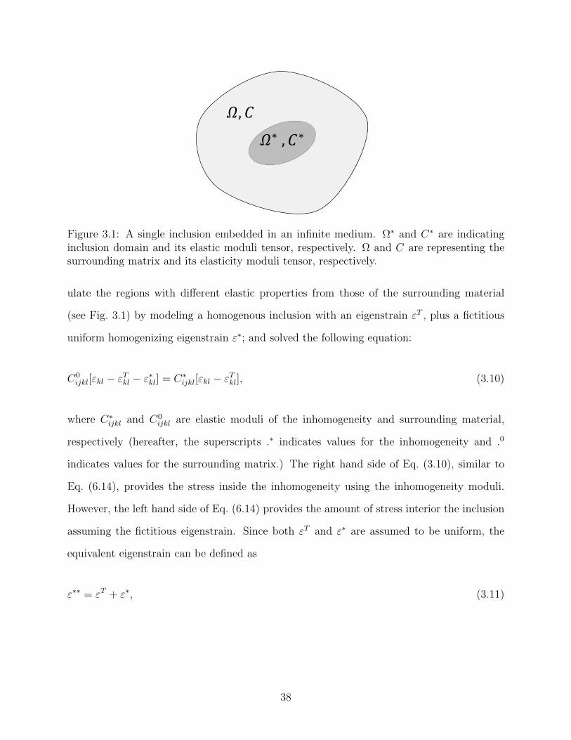
Figure 3.1: A single inclusion embedded in an infinite medium. Ω∗ and C∗ are indicatinginclusion domain and its elastic moduli tensor, respectively. Ω and C are representing thesurrounding matrix and its elasticity moduli tensor, respectively.

ulate the regions with different elastic properties from those of the surrounding material

(see Fig. 3.1) by modeling a homogenous inclusion with an eigenstrain εT , plus a fictitious

uniform homogenizing eigenstrain ε∗; and solved the following equation:

C0ijkl[εkl − εTkl − ε∗kl] = C∗ijkl[εkl − εTkl], (3.10)

where C∗ijkl and C0ijkl are elastic moduli of the inhomogeneity and surrounding material,

respectively (hereafter, the superscripts .∗ indicates values for the inhomogeneity and .0

indicates values for the surrounding matrix.) The right hand side of Eq. (3.10), similar to

Eq. (6.14), provides the stress inside the inhomogeneity using the inhomogeneity moduli.

However, the left hand side of Eq. (6.14) provides the amount of stress interior the inclusion

assuming the fictitious eigenstrain. Since both εT and ε∗ are assumed to be uniform, the

equivalent eigenstrain can be defined as

ε∗∗ = εT + ε∗, (3.11)

38

where for the interior points

εij = Sijklε∗∗kl , (3.12)

σij = C∗ijkl[εkl − εTkl]. (3.13)

By substituting Eq. (4.4) into Eq. (3.10), ε∗∗ can be determined from the following relation-

ship

C0ijkl[Sklmnε

∗∗mn − ε∗∗kl ] = C∗ijkl[Sklmnε

∗∗mn − εTkl]. (3.14)

Note that Eq. (4.6) consists of 6 linear equations containing six unknowns (ε∗∗). Solving

for ε∗∗ in Eq. (4.6), the stress and strain inside the inclusion can be calculated by Eqs. (4.4)

and (4.5). This method is valid for both isotropic and anisotropic inhomogeneous inclusions

embedded in an isotropic medium. Assuming anisotropic inhomogeneous inclusion, elastic

moduli C∗ijkl, C0ijkl and Sijkl in Eq. (4.6) are taken for the isotropic material (Mura, 1987).

Similar to Eq. (6.13), stress and strain for the exterior points can be calculated using the

fourth rank tensor Dijkl

εij(x) = Dijkl(x)ε∗kl, (3.15)

σij(x) = Cijklεkl(x), (3.16)

where ε∗ is determined from Eq. (3.10), and

Dijkl(x) =1

8π(1− ν)

ψ,klij − 2νδklφ,ij

− (1 − ν)[φ,kjδil + φ,kiδjl + φ,ljδik + φ,liδjk

]. (3.17)

39

Dijkl(x) is similar to the Eshelby’s tensor, but for the exterior points (Mura, 1987). Sec-

tion 3.9 provides the details of calculation for tensor D, ψ, and φ. If x ∈ Ω, then Dijkl(x) =

Sijkl.

3.4 Poroelastic Inclusions

Rudnicki (2002a) has solved the problem of an isotropic ellipsoidal poroelastic inhomogene-

ity embedded in an elastic medium, and presented numerical results to show the effect of

geometry and material properties on the stresses caused by a fluid pressure change in the

inclusion. Using Eqs. (6.8) and (6.14), he derived the relationship between the stress, strain

and pore pressure change inside the inclusion (see more details in Section 3.8). However,

this solution does not incorporate the possible anisotropy of poroelastic or elastic properties

of the inhomogeneity. Chen (2011) used EIM to model a hydrocarbon reservoir as an inho-

mogeneous isotropic poroelastic inclusion and investigated the the effect of change in pore

pressure and elastic properties of the reservoir on redistribution of stresses and deformation

within the reservoir.

We use a different approach to derive the stress and strain solution for anisotropic poroe-

lastic inclusions. According to the definition of eigenstrain as stress-free transformation

strain, poroelastic transformation strain due to the changes in pore pressure εT can be ob-

tained by setting σij = 0 in Eq. (3.5)

εTmn = C−1mnijαijp = Lmnijαijp, (3.18)

where Lmnij is the tensor of elastic compliances, inverse of Cmnij, is defined as the solution

of the following equation

LmnijCijkl =1

2(δmkδnl + δmlδnk). (3.19)

40

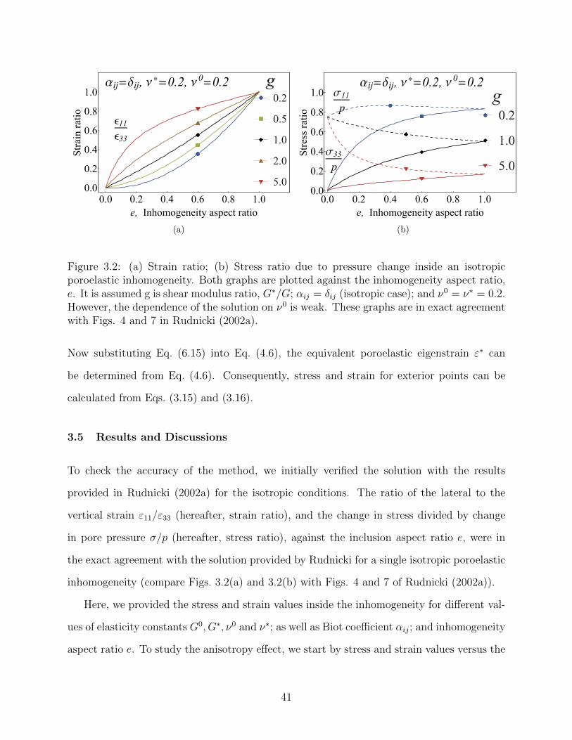
e11

e33

aij=dij, n*=0.2, n

0=0.2 g

0.2

0.5

1.0

2.0

5.0

0.0 0.2 0.4 0.6 0.8 1.0

0.0

0.2

0.4

0.6

0.8

1.0

e, Inhomogeneity aspect ratio

Str

ain

ratio

(a)

s33

p

s11

p

aij=dij, n*=0.2, n

0=0.2

g

0.2

1.0

5.0

0.0 0.2 0.4 0.6 0.8 1.00.0

0.2

0.4

0.6

0.8

1.0

e, Inhomogeneity aspect ratio

Str

ess

rati

o

(b)

Figure 3.2: (a) Strain ratio; (b) Stress ratio due to pressure change inside an isotropicporoelastic inhomogeneity. Both graphs are plotted against the inhomogeneity aspect ratio,e. It is assumed g is shear modulus ratio, G∗/G; αij = δij (isotropic case); and ν0 = ν∗ = 0.2.However, the dependence of the solution on ν0 is weak. These graphs are in exact agreementwith Figs. 4 and 7 in Rudnicki (2002a).

Now substituting Eq. (6.15) into Eq. (4.6), the equivalent poroelastic eigenstrain ε∗ can

be determined from Eq. (4.6). Consequently, stress and strain for exterior points can be

calculated from Eqs. (3.15) and (3.16).

3.5 Results and Discussions

To check the accuracy of the method, we initially verified the solution with the results

provided in Rudnicki (2002a) for the isotropic conditions. The ratio of the lateral to the

vertical strain ε11/ε33 (hereafter, strain ratio), and the change in stress divided by change

in pore pressure σ/p (hereafter, stress ratio), against the inclusion aspect ratio e, were in

the exact agreement with the solution provided by Rudnicki for a single isotropic poroelastic

inhomogeneity (compare Figs. 3.2(a) and 3.2(b) with Figs. 4 and 7 of Rudnicki (2002a)).

Here, we provided the stress and strain values inside the inhomogeneity for different val-

ues of elasticity constants G0, G∗, ν0 and ν∗; as well as Biot coefficient αij; and inhomogeneity

aspect ratio e. To study the anisotropy effect, we start by stress and strain values versus the

41

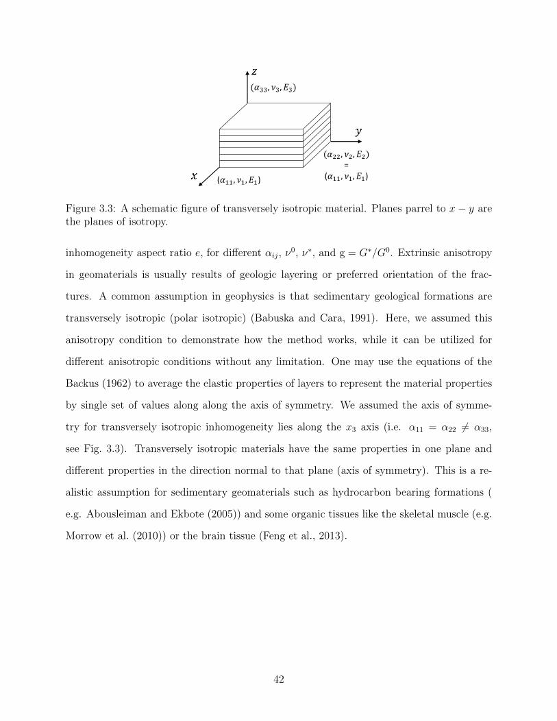
(𝛼33, 𝜈3, 𝐸3)

(𝛼22, 𝜈2, 𝐸2)=

(𝛼11, 𝜈1, 𝐸1)(𝛼11, 𝜈1, 𝐸1)

Figure 3.3: A schematic figure of transversely isotropic material. Planes parrel to x− y arethe planes of isotropy.

inhomogeneity aspect ratio e, for different αij, ν0, ν∗, and g = G∗/G0. Extrinsic anisotropy

in geomaterials is usually results of geologic layering or preferred orientation of the frac-

tures. A common assumption in geophysics is that sedimentary geological formations are

transversely isotropic (polar isotropic) (Babuska and Cara, 1991). Here, we assumed this

anisotropy condition to demonstrate how the method works, while it can be utilized for

different anisotropic conditions without any limitation. One may use the equations of the

Backus (1962) to average the elastic properties of layers to represent the material properties

by single set of values along along the axis of symmetry. We assumed the axis of symme-

try for transversely isotropic inhomogeneity lies along the x3 axis (i.e. α11 = α22 6= α33,

see Fig. 3.3). Transversely isotropic materials have the same properties in one plane and

different properties in the direction normal to that plane (axis of symmetry). This is a re-

alistic assumption for sedimentary geomaterials such as hydrocarbon bearing formations (

e.g. Abousleiman and Ekbote (2005)) and some organic tissues like the skeletal muscle (e.g.

Morrow et al. (2010)) or the brain tissue (Feng et al., 2013).

42

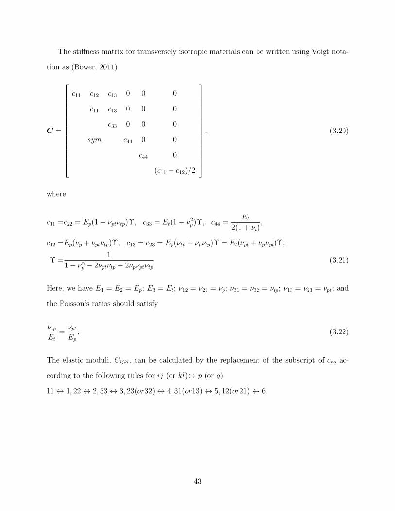
The stiffness matrix for transversely isotropic materials can be written using Voigt nota-

tion as (Bower, 2011)

C =

c11 c12 c13 0 0 0

c11 c13 0 0 0

c33 0 0 0

sym c44 0 0

c44 0

(c11 − c12)/2

, (3.20)

where

c11 =c22 = Ep(1− νptνtp)Υ, c33 = Et(1− ν2p)Υ, c44 =

Et2(1 + νt)

,

c12 =Ep(νp + νptνtp)Υ, c13 = c23 = Ep(νtp + νpνtp)Υ = Et(νpt + νpνpt)Υ,

Υ =1

1− ν2p − 2νptνtp − 2νpνptνtp

. (3.21)

Here, we have E1 = E2 = Ep; E3 = Et; ν12 = ν21 = νp; ν31 = ν32 = νtp; ν13 = ν23 = νpt; and

the Poisson’s ratios should satisfy

νtpEt

=νptEp. (3.22)

The elastic moduli, Cijkl, can be calculated by the replacement of the subscript of cpq ac-

cording to the following rules for ij (or kl)↔ p (or q)

11↔ 1, 22↔ 2, 33↔ 3, 23(or32)↔ 4, 31(or13)↔ 5, 12(or21)↔ 6.

43

For this materials Biot coefficient in the symmetry plane are equal, so the Biot coefficient

has the form

α =

α11 0 0

0 α11 0

0 0 α33

. (3.23)

Assuming isotropic elastic and transversely isotropic poroelastic conditions, the stress

ratio versus inhomogeneity aspect ratio, for various shear modulus ratios and different Pois-

son’s ratios are plotted in Fig. 3.4. The value of lateral and vertical stress ratio (σ11/p and

σ33/p) indicates how changes in pore fluid pressure may affect the total stress magnitude in

that direction. In transversely isotropic materials, the variation of the Biot coefficient in the

direction of the axis of symmetry α33, affects the vertical stress change more than lateral

stresses. Assuming the same values for Poisson’s ratio interior and exterior of the inhomo-

geneity to be ν0 = ν∗ = 0.2 (Figs. 3.4(a), 3.4(c) and 3.4(e)), the stress ratio in the lateral

direction is always higher than the stress ratio in the vertical direction (σ11/p > σ33/p).

However, by decreasing the anisotropy degree (as α33 → α11 = α22 = 1), the stress ratios

are approaching the same value for the spherical inhomogeneities (i.e. e = 1). Moreover, the

stress change ratio is higher in softer inhomogeneities. For example for a depleted aquifer,

the reduction in the total horizontal stress is more than reduction in the total vertical stress,

especially in softer inclusions.

The effect of Poisson’s ratio on the stress ratio is shown in Figs. 3.4(b), 3.4(d) and 3.4(e).

These plots show the weak dependency of vertical stress ratio to the Poisson’s ratio values,

whereas the lateral stress ratio decreases significantly for higher Poisson’s ratio values, which

is expected by intuition as materials with higher Poisson’s ratio are less compressible.

Figure 3.5 shows how anisotropy in the Biot coefficient changes the stress ratio distri-

bution inside and outside of the inclusion. For α33 < 1, we expect lower stress ratio since

lower Biot coefficient means less contribution of the pore pressure changes in the total stress

44

s33

p

s11

p

a11=a22=1, n*=0.2, n

0=0.2, g=0.2

a33

0.10 .25 0.50 .75 1.00

0.0 0.2 0.4 0.6 0.8 1.00.0

0.2

0.4

0.6

0.8

1.0

e, Inhomogeneity aspect ratio

Str

ess

rati

o

(a)

s33

p

s11

p

a11=a22=1, n0=0.2, n

*=0.4, g=0.2

a33

0.10 0.50 1.00

0.0 0.2 0.4 0.6 0.8 1.00.0

0.2

0.4

0.6

0.8

1.0

e, Inhomogeneity aspect ratio

Str

ess

rati

o

(b)

s33

p

s11

p

a11=a22=1, g=1

n*=0.2, n

0=0.2

a33

0.10 .25 0.50 .75 1.00

0.0 0.2 0.4 0.6 0.8 1.0

0.0

0.2

0.4

0.6

0.8

e, Inhomogeneity aspect ratio

Str

ess

rati

o

(c)

s33

p

s11

p

a11=a22=1, g=1

n0=0.2, n

*=0.4

a33

0.10 0.50 1.00

0.0 0.2 0.4 0.6 0.8 1.0

0.0

0.2

0.4

0.6

0.8

e, Inhomogeneity aspect ratio

Str

ess

rati

o

(d)

s33

p

s11

p

a11=a22=1, g=5

n*=0.2, n

0=0.2

a33

0.10 0.50 1.00

0.0 0.2 0.4 0.6 0.8 1.0

0.0

0.2

0.1

0.3

0.5

0.4

e, Inhomogeneity aspect ratio

Str

ess

rati

o

(e)

s33

p

s11

p

a11=a22=1, g=5

n0=0.2, n

*=0.4

a33

0.10 0.50 1.00

0.0 0.2 0.4 0.6 0.8 1.00.0

0.2

0.1

0.3

0.4

0.5

e, Inhomogeneity aspect ratio

Str

ess

rati

o

(f)

Figure 3.4: Stress ratio against inhomogeneity aspect ratio, e, for various shear modulusratio (g = G∗/G0) and Poisson’s ratio. The solid lines indicate vertical stress ratio σ33/p,whereas the dotted lines indicate lateral stress ratio σ11/p.

45

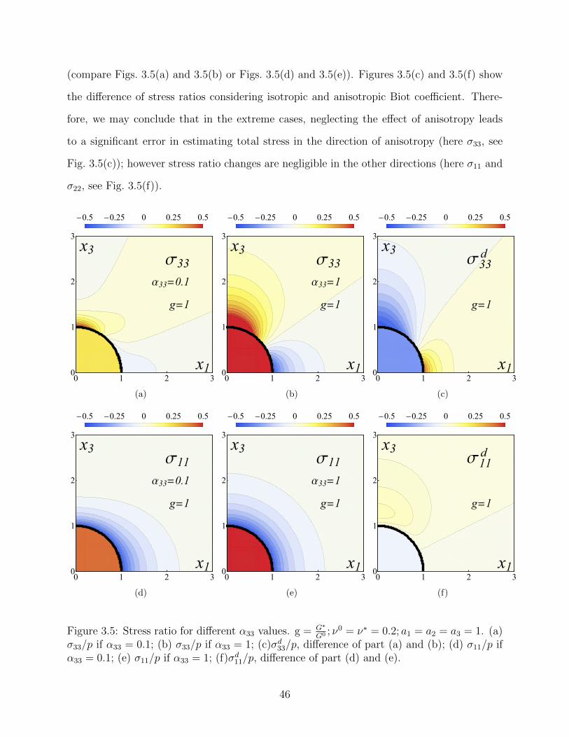
(compare Figs. 3.5(a) and 3.5(b) or Figs. 3.5(d) and 3.5(e)). Figures 3.5(c) and 3.5(f) show

the difference of stress ratios considering isotropic and anisotropic Biot coefficient. There-

fore, we may conclude that in the extreme cases, neglecting the effect of anisotropy leads

to a significant error in estimating total stress in the direction of anisotropy (here σ33, see

Fig. 3.5(c)); however stress ratio changes are negligible in the other directions (here σ11 and

σ22, see Fig. 3.5(f)).

-0.5 -0.25 0 0.25 0.5

s33

a33=0.1

g=1

x1

x3

0 1 2 30

1

2

3

(a)

-0.5 -0.25 0 0.25 0.5

s33

a33=1

g=1

x1

x3

0 1 2 30

1

2

3

(b)

-0.5 -0.25 0 0.25 0.5

s33

d

g=1

x1

x3

0 1 2 30

1

2

3

(c)

-0.5 -0.25 0 0.25 0.5

s11

a33=0.1

g=1

x1

x3

0 1 2 30

1

2

3

(d)

-0.5 -0.25 0 0.25 0.5

s11

a33=1

g=1

x1

x3

0 1 2 30

1

2

3

(e)

-0.5 -0.25 0 0.25 0.5

s11

d

g=1

x1

x3

0 1 2 30

1

2

3

(f)

Figure 3.5: Stress ratio for different α33 values. g = G∗

G0 ; ν0 = ν∗ = 0.2; a1 = a2 = a3 = 1. (a)σ33/p if α33 = 0.1; (b) σ33/p if α33 = 1; (c)σd33/p, difference of part (a) and (b); (d) σ11/p ifα33 = 0.1; (e) σ11/p if α33 = 1; (f)σd11/p, difference of part (d) and (e).

46

, , , , , , , , , , , , , , , , , , , , , , , , , , , , , , , ,

,

,

,

,

,

,

,

,

,,

,,

,,

,,

,,

, , , , , , , , , , , , , , , , , , , , , , , , , , , , , , , , , , , , , , , , , , , , , , , , ,

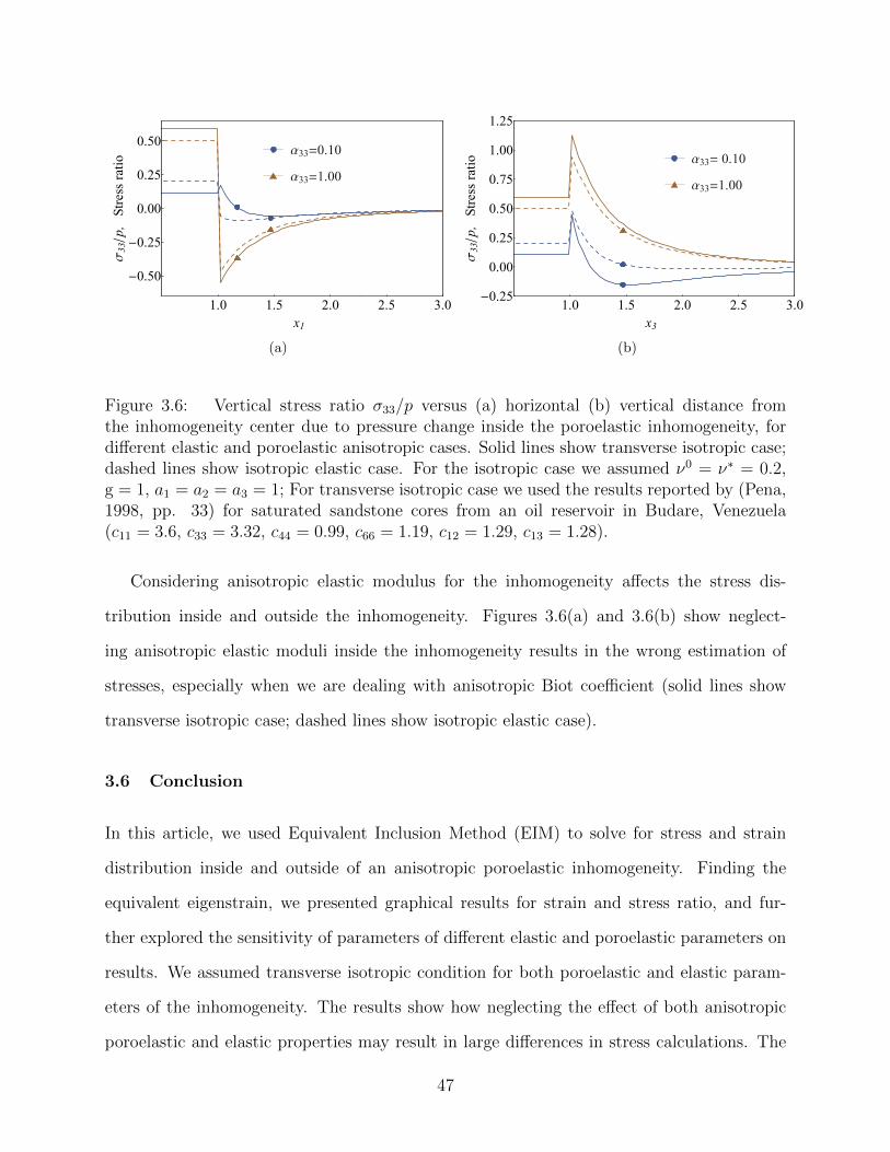
a11=a22=1, n*=0.2, n

0=0.2, g=1

a33=0.10

a33=1.00

1.0 1.5 2.0 2.5 3.0

0.00

-0.50

0.50

-0.25

0.25

x1

s33êp,

Str

ess

rati

o

(a)

, , , , , , , , , , , , , , , , , , , , , , , , , , , , , , , ,

,

,

,

,

,

,

,

,

,

,

,

,

,

,

,,

,,

,,

,,

,,

,,

, , , , , , , , , , , , , , , , , , , , , , , , , , , , , , , , , , , , , , , , ,

a33= 0.10

a33=1.00

1.0 1.5 2.0 2.5 3.0

0.00

1.00

0.50

-0.25

0.25

0.75

1.25

x3

s33êp,

Str

ess

rati

o

(b)

Figure 3.6: Vertical stress ratio σ33/p versus (a) horizontal (b) vertical distance fromthe inhomogeneity center due to pressure change inside the poroelastic inhomogeneity, fordifferent elastic and poroelastic anisotropic cases. Solid lines show transverse isotropic case;dashed lines show isotropic elastic case. For the isotropic case we assumed ν0 = ν∗ = 0.2,g = 1, a1 = a2 = a3 = 1; For transverse isotropic case we used the results reported by (Pena,1998, pp. 33) for saturated sandstone cores from an oil reservoir in Budare, Venezuela(c11 = 3.6, c33 = 3.32, c44 = 0.99, c66 = 1.19, c12 = 1.29, c13 = 1.28).

Considering anisotropic elastic modulus for the inhomogeneity affects the stress dis-

tribution inside and outside the inhomogeneity. Figures 3.6(a) and 3.6(b) show neglect-

ing anisotropic elastic moduli inside the inhomogeneity results in the wrong estimation of

stresses, especially when we are dealing with anisotropic Biot coefficient (solid lines show

transverse isotropic case; dashed lines show isotropic elastic case).

3.6 Conclusion

In this article, we used Equivalent Inclusion Method (EIM) to solve for stress and strain

distribution inside and outside of an anisotropic poroelastic inhomogeneity. Finding the

equivalent eigenstrain, we presented graphical results for strain and stress ratio, and fur-

ther explored the sensitivity of parameters of different elastic and poroelastic parameters on

results. We assumed transverse isotropic condition for both poroelastic and elastic param-

eters of the inhomogeneity. The results show how neglecting the effect of both anisotropic

poroelastic and elastic properties may result in large differences in stress calculations. The

47

stress ratio changes are much larger in the direction parallel to the axis of symmetry than

the directions in the plain of symmetry.

3.7 Calculating Dijkl

Suppose we have an ellipsoidal inhomogeneity Ω, with principal half axes a1, a2, and a3. The

strain and stress field at the point x = (x1, x2, x3), located outside of the inhomogeneity

(x ∈ D − Ω), can be expressed by

εij(x) = Dijkl(x)ε∗kl, (3.24)

σij(x) = Cijklεkl(x), (3.25)

where

Dijkl(x) =1

8π(1− ν)

ψ,klij − 2νδklφ,ij

− (1 − ν)[φ,kjδil + φ,kiδjl + φ,ljδik + φ,liδjk

], (3.26)

and ε∗ is homogenizing eigenstrain; Cijkl is elastic moduli of the surrounding medium; and

ν is the Poisson’s ratio of the inhomogeneity. For the complete derivation and more details

check Mura (1987).

In Eq. (3.26)

φ,ij = − δijII(λ)− xiII,J(λ) (3.27)

48

ψ,ijkl = − δijδkl[IK(λ)− a2IIIK(λ)]− (δikδjl + δjkδil)[IJ(λ)− a2

IIIJ(λ)]

− δijxk[IK(λ)− a2IIIK(λ)],l − (δikxj + δjkxi)[IJ(λ)− a2

IIIJ(λ)],l

− (δilxj + δjlxi)[IJ(λ)− a2IIIJ(λ)],k − xixj[IJ(λ)− a2

IIIJ(λ)],kl

(3.28)

where

Iij···(λ) = 2πa1a2a3

∫ ∞λ

ds

(a2i + s)(a2

j + s) · · ·∆(s)(3.29)

∆(s) =√

(a21 + s)(a2

2 + s)(a23 + s) (3.30)

and λ is the largest positive root of the equation

x21

a21 + λ

+x2

2

a22 + λ

+x2

3

a23 + λ

= 1. (3.31)

3.8 Results for Ellipsoidal Isotropic Poroelastic Inclusion

According to Rudnicki (2002a), if an isotropic solid is loaded by far field stresses σ∞ (or

strains, ε∞), the relation between the strains are

εImn + SmnkkεItt(k − g) + (g − 1)Smnklε

Ikl = ε∞mn −

1

3

αp

KSmnkk, (3.32)

where k = KI/K and g = GI/G; and superscripts and subscripts I designates the properties

of the inclusion.

In addition, the result for the stress relation can be rewritten by separating the stress

components to mean and deviatoric parts (σij = (σ/3)δij+qij) by the following two equations

49

qImn + (g − 1)

Smnkl −

Smnkl[(k − 1)Smnrr + δmn]

[3 + Srrtt(k − 1)]

qIkl

= gq∞mn −2GI

3K

[3Smnkk − Srrttδmn]

[3 + Srrtt(k − 1)](αp+ k − 1),

(3.33)

and

[1 +

Srrtt3

(k − 1)

]+ (g − 1)

KI

2GI

Smmklqkl = kσ∞ +

(1 +

Srrtt3αp

). (3.34)

3.9 A Discussion on the Effective Material Properties of the Medium

Methodology

Let’s assume that we have a medium consisted of poroelastic inclusions embedded in an

elastic matrix (see Fig. 3.7). Inclusions are assumed to have the same ellipsoidal shape and

material properties uniformly distributed in the medium; however, the material properties

of the inclusions could be different from that of the matrix. The ratio of the inclusions

volume VI to the total volume of the medium VM is supposed to be β (β = VI/VM). We

used the Eshelby technique (Eshelby, 1957, 1959) and the concept of average stress in the

matrix developed by Mori and Tanaka (1973) to determine the effective material properties

for this medium. We modified the existing methods available for elastic composites (Tandon

and Weng, 1984) and elastic porous materials (Zhao et al., 1989) to analyze the effective

material properties by adding the impact of poroelastic stress and strain caused by the pore

fluid pressure inside the inclusions.

Suppose that the medium is subjected to far-field stress σ0ij and excessive fluid pressure

p in the inclusions. The average elastic modulus of the medium (matrix with pressurized

inclusions) is represented by Cijkl; whereas C0ijkl and C1

ijkl are the matrix and inclusions

50

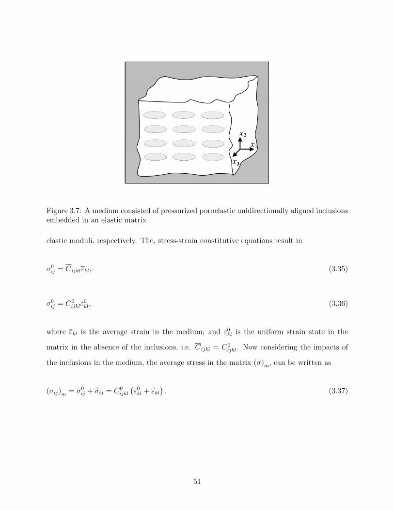
Figure 3.7: A medium consisted of pressurized poroelastic unidirectionally aligned inclusionsembedded in an elastic matrix

elastic moduli, respectively. The, stress-strain constitutive equations result in

σ0ij = Cijklεkl, (3.35)

σ0ij = C0

ijklε0kl, (3.36)

where εkl is the average strain in the medium; and ε0kl is the uniform strain state in the

matrix in the absence of the inclusions, i.e. Cijkl = C0ijkl. Now considering the impacts of

the inclusions in the medium, the average stress in the matrix (σ)m, can be written as

(σij)m = σ0ij + σij = C0

ijkl

(ε0kl + εkl

), (3.37)

51

where εij is the additional average perturbed strain from ε0ij caused by the presence of the

inclusions. Therefore, the corresponding stress σij can be written as

σij = C0ijklεkl. (3.38)

On the other hand, the total stress in the inclusions (σij)I , can be calculated by adding σpt

to (σ)m, where σpt is the perturbed stress component induced in the inclusion ( by pore

pressure and/or dissimilarity between material properties) from the average stress in the

matrix (σ)m. Based on these definitions, we have

(σij)I = (σij)m + σptij = σ0ij + σij + σptij . (3.39)

Using the equivalent inclusion method (EIM), the perturbed strain and stress components

in the inclusion may be calculated as (Eshelby, 1957)

εptij = Sijklε∗kl, (3.40)

σptij = C0ijkl[ε

ptkl − ε

∗kl], (3.41)

where Sijkl are the components of the Eshelby tensor. Here, ε∗ is the fictitious uniform

homogenizing eigenstrain and can be determined from solving the below system of equations

(σTij)I

= C1ijkl

(ε0kl + εkl + εptkl + εpkl

)= C0

ijkl

(ε0kl + εkl + εptkl − ε

∗kl

), (3.42)

52

where εp is the poroelastic transformation strain and can be obtained by setting σij = 0 in

the poroelastic constitutive equations

εpmn = −L1mnijα

1ijp. (3.43)

In Eq. (3.43), L1mnij is the elastic compliance tensor for the inclusions i.e. inverse of C1

mnij;

and α1ij is the Biot coefficient of the inclusion. Note that ε and ε∗kl are the only unknown

parameters in the system of Eq. (3.42). Considering the fact that the average stress over the

matrix and inclusion should be the same as the sum of the farfield stress σ0ij and the fluid

pore pressure in the inclusions, we have

σij + β(σptij + αpδij) = 0. (3.44)

Substituting Eqs. (3.40), (3.43) and (3.44) into Eq. (3.42), ε∗ can be determined from solving

the system of linear equations in Eq. (3.42). Finally, the average strain in the medium εkl,

can be calculated by volume averaging of the strain values in the inclusion and matrix.

Therefore, we have

εij = (1− β)(ε0ij + εij) + β(ε0

ij + εij + εptij )

= ε0ij + εij + βεptij .

(3.45)

Using Eqs. (3.36) and (3.45), the average elastic modulus of the medium Cijkl can be calcu-

lated from Eq. (3.35).

Numerical Results

To calculate the effective material constants of the medium, we applied the appropriate stress

at infinity and p inside the inclusions and calculated the corresponding average strains in

the medium.

53

Applying σ011 = 1 at infinity and p = 1 inside the inclusions, we calculated the average

directional Young modulus E11 as

σ011 = (E11)M ε11. (3.46)

Figure 3.8 shows the longitudinal Young’s modulus of the medium (E11)M ratio to Young’s

modulus of the matrix Em for different inhomogeneity aspect ratios R, volume ratios β

and material properties. Figures 3.8(a) to 3.8(c) are for the case of σ011 = p = 1. More-

over, Fig. 3.8(a) represents a case with softer inhomogeneities than the surrounding matrix,

whereas Fig. 3.8(c) represents a case with stiffer inhomogeneities. As we expect in the case

of no material properties discrepancy between the inclusions and the matrix, the inhomo-

geneity aspect ratio will not change the results. Figure 3.8(b) shows that the existence of

fluid pressure inside the inclusions causes decrease in longitudinal Young’s modulus.

The same approach can be used for determining other material constants for the trans-

verse isotopic poroelastic medium with pressurized inhomogeneities. For example similar to

(E11)M , the transverse Young’s modulus (E22)M can be determined as

σ022 = E22ε22. (3.47)

Since the fluid pore pressure impact is the same in all directions, substituting R with 1/R,

we will have (E22)M |R = (E11)M |1/R.

Figure 3.8(d) represents the impact of different fluid pressures in the inhomogeneities

(e.g. p = 0, 0.25, 0.75, 1 and 2). As shown in this figure, higher pore pressures , i.e. more

damage inside the medium, results in lower average stiffness.

3.10 References

Aadnoy, B., 1988. Modeling of the stability of highly inclined boreholes in anisotropic rockformations. SPE Drilling Engineering 3. doi:10.2118/16526-PA.

54

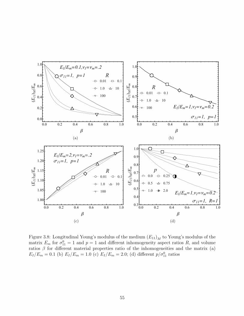
s11=1, p=1

EIêEm=0.1,nI=nm=.2

R

0.01 0.1

1.0 10

100

0.0 0.2 0.4 0.6 0.8 1.0

0.0

0.2

0.4

0.6

0.8

1.0

b

HE

11LM

êE

m

(a)

s11=1, p=1

EIêEm=1,nI=nm=0.2

R

0.01 0.1

1.0 10

100

0.0 0.2 0.4 0.6 0.8 1.0

0.5

0.6

0.7

0.8

0.9

1.0

bHE

11LM

êE

m

(b)

s11=1, p=1

EIêEm=2,nI=nm=.2

R

0.01 0.1

1.0 10

100

0.0 0.2 0.4 0.6 0.8 1.0

1.00

1.05

1.10

1.15

1.20

1.25

b

HE

11LM

êE

m

(c)

s11=1, R=1

EIêEm=1,nI=nm=0.2

p

0.0 0.25

0.5 0.75

1.0 2.0

0.0 0.2 0.4 0.6 0.8 1.00.3

0.4

0.5

0.6

0.7

0.8

0.9

1.0

b

HE

11LM

êE

m

(d)

Figure 3.8: Longitudinal Young’s modulus of the medium (E11)M to Young’s modulus of thematrix Em for σ0

11 = 1 and p = 1 and different inhomogeneity aspect ratios R, and volumeratios β for different material properties ratio of the inhomogeneities and the matrix (a)EI/Em = 0.1 (b) EI/Em = 1.0 (c) EI/Em = 2.0; (d) different p/σ0

11 ratios

55

Abousleiman, Y.N., Ekbote, S., 2005. Solutions for the inclined borehole in a porothermoe-lastic transversely isotropic medium. Journal of Applied Mechanics 72, 102. doi:10.1115/1.1825433.

Ahmadi, M., Dahi Taleghani, A., Sayers, C.M., 2014a. Direction dependence of frac-ture compliance induced by slickensides. GEOPHYSICS 79, C91–C96. doi:10.1190/geo2013-0227.1.

Ahmadi, M., Dahi Taleghani, A., Sayers, C.M., 2014b. Direction dependence of fracturecompliance ratio induced by slickensides. Accepted for Publication in Geophysics .

Amadei, B., 1996. Importance of anisotropy when estimating and measuring in situ stressesin rock. International Journal of Rock Mechanics and Mining Sciences & GeomechanicsAbstracts 33, 293–325. doi:10.1016/0148-9062(95)00062-3.

Aoki, T., Tan, C., Bamford, W., 1993. Effects of deformation and strength anisotropy onborehole failures in saturated shales. International Journal of Rock Mechanics and MiningSciences & Geomechanics Abstracts 30, 1031–1034. doi:10.1016/0148-9062(93)90067-N.

Babuska, V., Cara, M., 1991. Seismic anisotropy in the Earth. Springer.

Backus, G.E., 1962. Long-wave elastic anisotropy produced by horizontal layering. Journalof Geophysical Research 67, 4427–4440. doi:10.1029/JZ067i011p04427.

Bang, J., Solstad, A., Mjaaland, S., 2001. Formation electrical anisotropy derived frominduction-log measurements in a horizontal well. SPE Reservoir Evaluation & Engineering4, 483–488. doi:10.2118/75115-PA.

Bedayat, H., Dahi Taleghani, A., 2012. Drainage of poroelastic fractures and its implica-tions on the performance of naturally fractured reservoirs, in: 46th US Rock Mechan-ics/Geomechanics Symposium, Chicago, IL, USA.

Bedayat, H., Dahi Taleghani, A., 2013. The equivalent inclusion method for poroelasticityproblems, in: Poromechanics V, American Society of Civil Engineers, Reston, VA. pp.1279–1288. doi:10.1061/9780784412992.153.

Bedayat, H., Dahi Taleghani, A., 2014. Interacting double poroelastic inclusions. Mechanicsof Materials 69, 204–212. doi:10.1016/j.mechmat.2013.10.006.

56

Berryman, J.G., 1992. Effective stress for transport properties of inhomogeneous porousrock. Journal of Geophysical Research 97, 17409. doi:10.1029/92JB01593.

Berryman, J.G., 1997. Generalization of Eshelby’s formula for a single ellipsoidal elasticinclusion to poroelasticity and thermoelasticity. Physical Review Letters 79, 1142–1145.doi:10.1103/PhysRevLett.79.1142.

Berryman, J.G., 2011. Mechanics of layered anisotropic poroelastic media with applicationsto effective stress for fluid permeability. International Journal of Engineering Science 49,122–139. doi:10.1016/j.ijengsci.2010.06.027.

Biot, M.A., 1941. General theory of three-dimensional consolidation. Journal of AppliedPhysics 12, 155. doi:10.1063/1.1712886.

Biot, M.A., 1955. Theory of elasticity and consolidation for a porous anisotropic solid.Journal of Applied Physics 26, 182. doi:10.1063/1.1721956.

Bower, A.F., 2011. Applied mechanics of solids. CRC Press.

Bruschke, M.V., Advani, S.G., 1990. A finite element/control volume approach to moldfilling in anisotropic porous media. Polymer Composites 11, 398–405. doi:10.1002/pc.750110613.

Cederbaum, G., Li, L., Schulgasser, K., 2000. Poroelastic structures. Elsevier.

Chen, Z.R., 2011. Poroelastic model for induced stresses and deformations in hydrocar-bon and geothermal reservoirs. Journal of Petroleum Science and Engineering 80, 41–52.doi:10.1016/j.petrol.2011.10.004.

Cheng, A.H.D., 1997. Material coefficients of anisotropic poroelasticity. International Jour-nal of Rock Mechanics and Mining Sciences 34, 199–205. doi:10.1016/S0148-9062(96)00055-1.

Cheng, A.H.D., Abousleiman, Y.N., Detournay, E., Cui, L., Roegiers, J.C., 1996. Mandel’sproblem revisited. Geotechnique 46, 187–195. doi:10.1680/geot.1996.46.2.187.

57

Cowin, S.C., 1999. Bone poroelasticity. Journal of Biomechanics 32, 217–238. doi:10.1016/S0021-9290(98)00161-4.

Cowin, S.C., Doty, S.B., 2007. Tissue mechanics. Springer New York, New York, NY.doi:10.1007/978-0-387-49985-7.

Crampin, S., 1994. The fracture criticality of crustal rocks. Geophysical Journal International118, 428–438. doi:10.1111/j.1365-246X.1994.tb03974.x.

Cui, L., Cheng, A.H.D., Kaliakin, V.N., Abousleiman, Y.N., Roegiers, J.c., 1996. Finiteelement analysis of anisotropic poroelasticity: a generalized Mandel’s problem and aninclined borehole problem. International Journal for Numerical and Analytical Meth-ods in Geomechanics 20, 381–401. doi:10.1002/(SICI)1096-9853(199606)20:6<381::AID-NAG826>3.0.CO;2-Y.

Dahi Taleghani, A., Ahmadi, M., Olson, J.E., Wang, W., 2014. Thermal reactivation ofmicrofractures and its potential impact on hydraulic fractures efficiency. Accepted forpublication in SPE Journal .

Dahi Taleghani, A., Olson, J.E., 2011. Numerical modeling of multistranded-hydraulic-fracture propagation: Accounting for the interaction between induced and natural frac-tures. SPE Journal , 575–581.

Detournay, E., Cheng, A.H.D., 1991. Plane strain analysis of a stationary hydraulic fracturein a poroelastic medium. International Journal of Solids and Structures 27, 1645–1662.doi:10.1016/0020-7683(91)90067-P.

Dormieux, L., Kondo, D., Ulm, F.J., 2006. Microporomechanics. John Wiley & Sons, Ltd,Chichester, UK. doi:10.1002/0470032006.

Eshelby, J.D., 1957. The determination of the elastic field of an ellipsoidal inclusion, andrelated problems. Proceedings of the Royal Society A: Mathematical, Physical and Engi-neering Sciences 241, 376–396. doi:10.1098/rspa.1957.0133.

Eshelby, J.D., 1959. The elastic field outside an ellipsoidal inclusion, in: Proceedings of theRoyal Society of London. Series A, Mathematical and Physical, pp. 561–569.

58

Eshelby, J.D., 1961. Elastic inclusions and inhomogeneities, in: Sneddon, I.N., Hill, R.(Eds.), Progress in Solid Mechanics, Vol.2. North-Holland, Amsterdam, pp. 89–140.

Feng, Y., Okamoto, R.J., Namani, R., Genin, G.M., Bayly, P.V., 2013. Measurements ofmechanical anisotropy in brain tissue and implications for transversely isotropic materialmodels of white matter. Journal of the mechanical behavior of biomedical materials 23,117–32. doi:10.1016/j.jmbbm.2013.04.007.

Ferrari, M., 2000. Nanomechanics, and biomedical nanomechanics: Eshelby’s inclusion andinhomogeneity problems at the discrete/continuum interface. Biomedical Microdevices ,273–281doi:10.1023/A:1009903205275.

Ghabezloo, S., Hemmati, S., 2011. Poroelasticity of a micro-heterogeneous material saturatedby two immiscible fluids. International Journal of Rock Mechanics and Mining Sciences48, 1376–1379. doi:10.1016/j.ijrmms.2011.10.003.

He, Z., Caratini, G., Dormieux, L., Kondo, D., 2013. Homogenization of anisotropic elasto-plastic behaviors of a porous polycrystal with interface effects , 3213–3236doi:10.1002/nag.

Hellmich, C., Ulm, F.j., 2002. Micromechanical model for ultrastructural stiffness of min-eralized tissues. Journal of Engineering Mechanics 128, 898–908. doi:10.1061/(ASCE)0733-9399(2002)128:8(898).

Hu, D.W., Zhou, H., Shao, J.F., 2013. An anisotropic damage-plasticity model for saturatedquasi-brittle materials. International Journal for Numerical and Analytical Methods inGeomechanics 37, 1691–1710. doi:10.1002/nag.2103.

Hudson, J.A., 1981. Wave speeds and attenuation of elastic waves in material containingcracks. Geophysical Journal International 64, 133–150. doi:10.1111/j.1365-246X.1981.tb02662.x.

Kanj, M., Abousleiman, Y.N., Ghanem, R., 2003. Poromechanics of anisotropic hol-low cylinders. Journal of Engineering Mechanics 129, 1277–1287. doi:10.1061/(ASCE)0733-9399(2003)129:11(1277).

59

Khan, S., Ansari, S., Han, H., Khosravi, N., 2011. Importance of shale anisotropy in esti-mating in-situ stresses and wellbore stability analysis in Horn River Basin, in: Proceed-ings of Canadian Unconventional Resources Conference, Society of Petroleum Engineers.doi:10.2118/149433-MS.

Khan, S., Williams, R., Ansari, S., Khosravi, N., 2012. Impact of mechanical anisotropyon design of hydraulic fracturing in shales, in: Proceedings of Abu Dhabi InternationalPetroleum Conference and Exhibition, Society of Petroleum Engineers. doi:10.2118/162138-MS.

Khoshgofta, M., Najarian, S., Farmanzad, F., Vahidi, B., Ghomshe, F.T., 2007. A biome-chanical composite model to determine effective elastic moduli of the CNS Gray Matter.American Journal of Applied Sciences 4, 918–924. doi:10.3844/ajassp.2007.918.924.

Levasseur, S., Collin, F., Charlier, R., Kondo, D., 2013. On micromechanical damage model-ing in geomechanics: Influence of numerical integration scheme. Journal of Computationaland Applied Mathematics 246, 215–224. doi:10.1016/j.cam.2012.05.022.

Levin, V.M., Alvarez-Tostado, J.M., 2003. Eshelby’s formula for an ellipsoidal elastic inclu-sion in anisotropic poroelasticity and thermoelasticity. International Journal of Fracture119/120, L77–L82. doi:10.1023/A:1024907500335.

Li, L., Shirazi-Adl, A., Buschmann, M.D., 2003. Investigation of mechanical behavior ofarticular cartilage by fibril reinforced poroelastic models. Biorheology 40, 227–33.

Li, S., Sauer, R.a., Wang, G., 2007. The Eshelby tensors in a finite pherical domain-Part I:theoretical formulations. Journal of Applied Mechanics 74, 770. doi:10.1115/1.2711227.

Li, S., Wang, G., 2008. Introduction to micromechanics and nanomechanics. World Scientific.

Litewka, a., 2003. Load-induced oriented damage and anisotropy of rock-like materials.International Journal of Plasticity 19, 2171–2191. doi:10.1016/S0749-6419(03)00064-0.

Malekmotiei, L., Farahmand, F., Shodja, H.M., Samadi-Dooki, A., 2013. An analytical ap-proach to study the intraoperative fractures of femoral shaft during total hip arthroplasty.Journal of biomechanical engineering 135, 41004. doi:10.1115/1.4023699.

60

Marquez, J.P., Genin, G.M., Zahalak, G.I., Elson, E.L., 2005. Thin bio-artificial tissues inplane stress: the relationship between cell and tissue strain, and an improved constitutivemodel. Biophysical journal 88, 765–77. doi:10.1529/biophysj.104.040808.

Mehrabian, A., Abousleiman, Y.N., 2013. Generalized poroelastic wellbore problem. Inter-national Journal for Numerical and Analytical Methods in Geomechanics doi:10.1002/nag.2160.

Moran, J.H., Gianzero, S., 1979. Effects of formation anisotropy on resistivitylogging mea-surements. GEOPHYSICS 44, 1266–1286. doi:10.1190/1.1441006.

Mori, T., Tanaka, K., 1973. Average stress in matrix and average elastic energy of materialswith misfitting inclusions. Acta Metallurgica 21, 571–574. doi:10.1016/0001-6160(73)90064-3.

Morrow, D.A., Haut Donahue, T.L., Odegard, G.M., Kaufman, K.R., 2010. Transverselyisotropic tensile material properties of skeletal muscle tissue. Journal of the mechanicalbehavior of biomedical materials 3, 124–9. doi:10.1016/j.jmbbm.2009.03.004.

Mueller, M.C., 1991. Prediction of lateral variability in fracture intensity using multi-component shear-wave surface seismic as a precursor to horizontal drilling in the AustinChalk. Geophysical Journal International 107, 409–415. doi:10.1111/j.1365-246X.1991.tb01402.x.

Mura, T., 1987. Micromechanics of defects in solids. Martinus Nijhoff Publishers.

Nemat-Nasser, S., Hori, M., 1999. Micromechanics: overall properties of heterogeneousmaterials. Elsevier, Amsterdam.

Nowinski, J.L., Davis, C.F., 1970. A model of the human skull as a poroelastic sphericalshell subjected to a quasistatic load. Mathematical Biosciences 8, 397–416. doi:10.1016/0025-5564(70)90120-3.

Nur, A., Simmons, G., 1969. Stress-induced velocity anisotropy in rock: An experimentalstudy. Journal of Geophysical Research 74, 6667–6674. doi:10.1029/JB074i027p06667.

Pena, F.J.R., 1998. Elastic properties of sedimentary anisotropic rocks (measurments andapplicatiosn). Ph.D. thesis. Massachusetts Institute of Technology.

61

Pollard, D.D., Fletcher, R.C., 2005. Fundamentals of structural geology. Cambridge Univer-sity Press.

Rawal, C., Ghassemi, A., 2014. A reactive thermo-poroelastic analysis of water injection intoan enhanced geothermal reservoir. Geothermics 50, 10–23. doi:10.1016/j.geothermics.2013.05.007.

Rice, J.R., Cleary, M.P., 1976. Some basic stress diffusion solutions for fluid-saturatedelastic porous media with compressible constituents. Reviews of Geophysics 14, 227.doi:10.1029/RG014i002p00227.

Rickman, J.M., 2009. The role of elastic anisotropy in poroelastic transport. Journal ofApplied Physics 106, 044911. doi:10.1063/1.3204649.

Rudnicki, J.W., 2002a. Alteration of regional stress by reservoirs and other inhomo- geneities:Stabilizing or destabilizing?, in: Vouille, G., Berest, P. (Eds.), Proc. 9th Int. Congr. RockMechanics,Vol. 3, Paris, Aug. 25-29, 1999, Paris, France. pp. 1629– 1637.

Rudnicki, J.W., 2002b. Eshelby transformations, pore pressure and fluid mass changes, andsubsidence, in: Poromechanics II, Proc. 2nd Biot Conference on Poromechanics, Grenoble,France.

Rutqvist, J., Wu, Y.S., Tsang, C.F., Bodvarsson, G., 2002. A modeling approach for analysisof coupled multiphase fluid flow, heat transfer, and deformation in fractured porous rock.International Journal of Rock Mechanics and Mining Sciences 39, 429–442. doi:10.1016/S1365-1609(02)00022-9.

Sayers, C.M., 1994. The elastic anisotrophy of shales. Journal of Geophysical Research 99,767. doi:10.1029/93JB02579.

Sayers, C.M., 2005. Seismic anisotropy of shales. Geophysical Prospecting 53, 667–676.doi:10.1111/j.1365-2478.2005.00495.x.

Schoenberg, M., Sayers, C.M., 1995. Seismic anisotropy of fractured rock. GEOPHYSICS60, 204–211. doi:10.1190/1.1443748.

Shao, J.F., 1998. Poroelastic behaviour of brittle rock materials with anisotropic damage.Mechanics of Materials 30, 41–53. doi:10.1016/S0167-6636(98)00025-8.

62

Shao, J.F., Chau, K., Feng, X., 2006. Modeling of anisotropic damage and creep deformationin brittle rocks. International Journal of Rock Mechanics and Mining Sciences 43, 582–592.doi:10.1016/j.ijrmms.2005.10.004.

Shodja, H.M., Ojaghnezhad, F., 2007. A general unified treatment of lamellar inhomo-geneities. Engineering Fracture Mechanics 74, 1499–1510. doi:10.1016/j.engfracmech.2006.08.016.

Shodja, H.M., Rad, I., Soheilifard, R., 2003. Interacting cracks and ellipsoidal inhomo-geneities by the equivalent inclusion method. Journal of the Mechanics and Physics ofSolids 51, 945–960. doi:10.1016/S0022-5096(02)00106-0.

Shojaei, A., Dahi Taleghani, A., Li, G., 2014. A continuum damage failure model forhydraulic fracturing of porous rocks. International Journal of Plasticity doi:10.1016/j.ijplas.2014.03.003.

Soltanzadeh, H., Hawkes, C.D., 2012. Evaluation of caprock integrity during pore pressurechange using a probabilistic implementation of a closed-form poroelastic model. Interna-tional Journal of Greenhouse Gas Control 7, 30–38. doi:10.1016/j.ijggc.2011.10.006.

Soltanzadeh, H., Hawkes, C.D., Sharma, J.S., 2007. poroelastic model for production-and injection-induced stresses in reservoirs with elastic properties different from the sur-rounding rock. International Journal of Geomechanics 7, 353–361. doi:10.1061/(ASCE)1532-3641(2007)7:5(353).

Tan, X., Konietzky, H., 2014. Numerical study of variation in Biot’s coefficient with respectto microstructure of rocks. Tectonophysics 610, 159–171. doi:10.1016/j.tecto.2013.11.014.

Tandon, G.P., Weng, G.J., 1984. The effect of aspect ratio of inclusions on the elasticproperties of unidirectionally aligned composites. Polymer Composites 5, 327–333. doi:10.1002/pc.750050413.

Teklu, T.W., Graves, R., Tutuncu, A.N., Kazemi, H., Alameri, W., Alsumaiti, A., 2012.Geomechanics considerations in enhanced oil recovery, in: Proceedings of SPE Cana-dian Unconventional Resources Conference, Society of Petroleum Engineers. doi:10.2118/162701-MS.

63

Turner, C., Chandran, A., Pidaparti, R., 1995. The anisotropy of osteonal bone and itsultrastructural implications. Bone 17, 85–89. doi:10.1016/8756-3282(95)00148-7.

Verruijt, A., 2014. Theory and problems of poroelasticity. Delf University of Technology.

Voyiadjis, G.Z., Kattan, P.I., 2006. Advances in damage mechanics: metals and metal matrixcomposites with an introduction to fabric tensors, 2nd Edition, in: Advances in DamageMechanics: Metals and Metal Matrix Composites With an Introduction to Fabric Tensors,2nd Edition. second edi ed.. Elsevier Science Ltd, Oxford, p. 740.

Wang, H., Towler, B., Soliman, M., 2007. Near wellbore stress analysis and wellbore strength-ening for drilling depleted formations, in: Proceedings of Rocky Mountain Oil & Gas Tech-nology Symposium, Society of Petroleum Engineers. pp. 1–12. doi:10.2118/102719-MS.

Wang, H.F., 2000. Theory of linear poroelasticity with applications to geomechanics andhydrogeology. Princeton University Press.

Wu, J., Herzog, W., Epstein, M., 1999. Modelling of location- and time-dependent defor-mation of chondrocytes during cartilage loading. Journal of Biomechanics 32, 563–572.doi:10.1016/S0021-9290(99)00034-2.

Zhao, Y.H., Tandon, G.P., Weng, G.J., 1989. Elastic moduli for a class of porous materials.Acta Mechanica 76, 105–131. doi:10.1007/BF01175799.

Zhou, K., Hoh, H.J., Wang, X., Keer, L.M., Pang, J.H., Song, B., Wang, Q.J., 2013. Areview of recent works on inclusions. Mechanics of Materials 60, 144–158. doi:10.1016/j.mechmat.2013.01.005.

Zhou, K., Keer, L.M., Jane Wang, Q., Ai, X., Sawamiphakdi, K., Glaws, P., Paire, M., Che,F., 2012. Interaction of multiple inhomogeneous inclusions beneath a surface. ComputerMethods in Applied Mechanics and Engineering 217-220, 25–33. doi:10.1016/j.cma.2012.01.006.

Zhou, X., Ghassemi, A., 2011. Three-dimensional poroelastic analysis of a pressurized nat-ural fracture. International Journal of Rock Mechanics and Mining Sciences 48, 527–534.doi:10.1016/j.ijrmms.2011.02.002.

64

Zou, W., He, Q., Huang, M., Zheng, Q., 2010. Eshelby’s problem of non-elliptical inclusions.Journal of the Mechanics and Physics of Solids 58, 346–372. doi:10.1016/j.jmps.2009.11.008.

65

Chapter 4Eshelby Solution for Double EllipsoidalInhomogeneities: Applications in Geo-science

We developed a method and presented it as a Mathematica code to calculate the stress and

strain fields inside and outside of two interacting ellipsoidal inhomogeneities with arbitrary

orientation with respect to each other, using the Eshelby technique. The Eshelby technique

can be used to determine the elastic fields in and around these inhomogeneities. Assuming

same material properties for one of the inclusions and the surrounding matrix, this code can

be also used for the single inhomogeneity problem. Different geological features like faults

and aquifers can be modeled as inhomogeneous inclusions.

We start by reviewing Eshelby’s solution for a single inclusion, a single inhomogeneity and

double inhomogeneity problem with the required formulation to calculate Eshelby tensors.

Then, we describe our code structure and validate it with existing solutions in the literature

and present numerical solutions.

4.1 Introduction

Determining the elastic fields inside and outside of inhomogeneities has many applications in

the geoscience, material science, and biomechanics. In geomechanics, the stress distribution

in and around reservoirs, aquifers, intrusions, fault zones, caverns, dikes, compaction bands,

and underground structures has been calculated using the Eshelby technique (Rudnicki,

66

2011). These geological structures may have different material properties and different strain

conditions (e.g. different pressure, temperature, or inelastic deformations) rather than that

of their surroundings. Rudnicki (2002a,b); Walsh (2002); Soltanzadeh et al. (2007); Chen

(2011); Soltanzadeh and Hawkes (2012); Bedayat and Dahi Taleghani (2013, 2014a,b) are

some examples of using Eshelby technique to calculate stress changes due to fluid injection

or withdrawal.

An inhomogeneity is defined as a sub-volume of the medium, that has different material

properties from those of its surroundings, whereas an inclusion is a finite sub-volume of a

medium, which may undergo different strain status from that of the surrounding environ-

ment. If a finite sub-volume of a medium experiences both of the above conditions at the

same time, it would be considered as an inhomogeneous inclusion. Hereafter, we use the

term inhomogeneity instead of inhomogeneous inclusion.

Eshelby (1957, 1959) formulated the elastic fields generated by an ellipsoidal inhomogene-

ity in an isotropic elastic infinite medium, which undergoes a uniform strain. This solution

implies that the stress and strain distribution inside an ellipsoidal inhomogeneity is uniform,

if the applied strains in the absence of the surrounding material, i.e. eigenstrain, is uni-

form. Elastic and plastic strains, pressure changes, and thermal expansions are examples of

different types of strains, which could be referred to as eigenstrains (Mura, 1987).

Existence of inhomogeneities in a material, changes the overall response and the elastic

field in the material. The problem of interacting inhomogeneities have been studied exten-

sively in the past decades. For example, Horii and Nemat-Nasser (1985) used the method

of pseudotractions to calculate the stress and strain fields in a linearly elastic homogeneous

solid which contains 2D inhomogeneities; Honein et al. (1992) solved analytically the in-

teraction of two 2D inclusions under anti-plane shear. For 3D interacting inhomogeneities,

Moschovidis and Mura (1975) used the Equivalent Inclusion Method (EIM) and the super-

position principal along Taylor series expansion to solve the two ellipsoidal inhomogeneities

problem; Kachanov and Laures (1989) solved the problem of closely spaced, strongly inter-

67

acting penny shape cracks. Later, the computational efficiency of Moschovidis and Mura

(1975) solution for interactive inclusions was improved by Shodja et al. (2003); and the solu-

tion was further modified to solve poroelastic isotropic (Bedayat and Dahi Taleghani, 2014a,

2013) and poroelastic anisotropic (Bedayat and Dahi Taleghani, 2014b) inhomogeneities.

The Eshelby’s method has been also utilized to solve more complex problems like lamellar

inhomogeneities (Shodja and Ojaghnezhad, 2007), inclusions in finite media (Li et al., 2007),

non-ellipsoidal inclusions (Zou et al., 2010), , inclusions in half-space (Zhou et al., 2012), or

analysis to simulate elasto-plastic large deformations of composites (Shojaei and Li, 2013).

See Zhou et al. (2013) for an extensive review on the subject.

Healy (2009) published a code for calculation and visualisation of the internal and external

elastic fields for spheroidal inclusions. Later, Meng et al. (2012) published a code for elastic

fields generated by an ellipsoidal inhomogeneity under remote in-situ stresses. We developed

a Mathematica code that calculates the stress and strain fields inside and outside a general

double ellipsoidal inhomogeneity problem. Assuming same material properties for one of the

inclusions and the surrounding matrix, this code can be also used for a single inhomogeneity

problem (see Section 4.7).

The outline of this paper is as follows: Section 4.2 reviews the Eshelby’s solution for the

single inclusion, the single inhomogeneity and the double inhomogeneity problem. Then in

Section 4.3, the formulation required to calculate the Eshelby tensor is provided for a single

ellipsoidal inclusion. In Section 4.4, we described the code structure. Finally, we verified our

code with existing solutions and presented a numerical example in Section 4.5.

4.2 Theory

4.2.1 Single inclusion

Consider an ellipsoidal inclusion in an infinite elastic solid, which undergoes a uniform eigen-

strain εTij (see Fig. 4.1). Eshelby (1957, 1959) showed that the actual strain and stress inside

68

𝒙𝟏

𝒙𝟐

𝒙𝟑

Figure 4.1: An ellipsoidal inclusion with principal axis parallel to Cartesian coordinatesystem (x1, x2, x3)

the inclusion are uniform and given by

εij = SijklεTkl, (4.1)

σij = C0ijkl[εkl − εTkl], (4.2)

where εij and σij are the components of strain and stress tensors in the matrix, respectively;

C0ijkl is the elastic moduli of the matrix; Eshelby tensor Sijkl, is a fourth rank tensor which

is a function of geometry and Poisson’s ratio of the ellipsoidal inclusion.

We provided the details to calculate the Eshelby tensor in Section 4.9 (see Mura (1987)

for more details).

4.2.2 Single inhomogeneity

Considering a fictitious uniform homogenizing eigenstrain ε∗, EIM can be used to determine

the stress and strain in inhomogeneities. EIM solves the inhomogeneity problem by modeling

a homogenous inclusion which undergoes fictitious uniform homogenizing eigenstrain ε∗, plus

69

an external transformation strain εT , which is the transformation strain. Defining ε∗∗ to be

ε∗∗ = εT + ε∗, (4.3)

the actual strain and stress inside of the inhomogeneity are

εij = Sijklε∗∗kl , (4.4)

σij = C1ijkl[εkl − εTkl], (4.5)

where C1ijkl is the elasticity tensor of the inhomogeneity; and ε∗ can be calculated from

solving the following equation

C0ijkl[Sklmnε

∗∗mn − ε∗∗kl ] = C1

ijkl[Sklmnε∗∗mn − εTkl]. (4.6)

For the exterior points, stress and strain fields can be calculated by substituting the fourth

rank tensor Dijkl for Sijkl in Eq. (4.4). Dijkl(x) is similar to Eshelby’s tensor, but for the

exterior points. If x ∈ Ω, then Dijkl(x) = Sijkl (Mura, 1987, p. 87). See Section 4.3 for more

details.

4.2.3 Double interacting inclusions

Moschovidis and Mura (1975) solved the stress field caused by two interacting inhomo-

geneities (Ω1 and Ω2) embedded in an infinite elastic medium (see Fig. 4.2) by writing EIM

equations for each inhomogeneity individually. Hence, the system of consistency equations

for two inhomogeneities under the applied stress σ0ij (similar to equation Eq. (4.6) for a single

inclusion), will be

C1ijkl[ε

0kl + ε1

kl + ε2kl] = C0

ijkl[ε0kl + ε1

kl + ε2kl − ε1∗

kl ] in Ω1, (4.7)

70

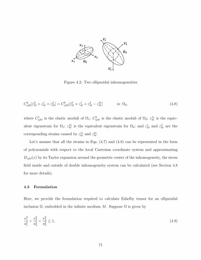
𝒙𝟐

𝒙𝟑

𝒙𝟏

𝒙𝟐

𝒙𝟑

𝒙𝟏 𝛀𝟏

𝛀𝟐

Figure 4.2: Two ellipsoidal inhomogeneities

C2ijkl[ε

0kl + ε1

kl + ε2kl] = C0

ijkl[ε0kl + ε1

kl + ε2kl − ε2∗

kl ] in Ω2, (4.8)

where C1ijkl is the elastic moduli of Ω1; C2

ijkl is the elastic moduli of Ω2; ε1∗kl is the equiv-

alent eigenstrain for Ω1; ε2∗kl is the equivalent eigenstrain for Ω2; and ε1

kl and ε2kl are the

corresponding strains caused by ε1∗kl and ε2∗

kl .

Let’s assume that all the strains in Eqs. (4.7) and (4.8) can be represented in the form

of polynomials with respect to the local Cartesian coordinate system and approximating

Dijkl(x) by its Taylor expansion around the geometric center of the inhomogeneity, the stress

field inside and outside of double inhomogeneity system can be calculated (see Section 4.8

for more details).

4.3 Formulation

Here, we provide the formulation required to calculate Eshelby tensor for an ellipsoidal

inclusion Ω, embedded in the infinite medium M . Suppose Ω is given by

x21

a21

+x2

2

a22

+x2

3

a23

≤ 1, (4.9)

71

where ai (i = 1, 2, and 3) are size of the principal half axis of the ellipsoidal inclusion.

According to Mura (1987) strain fields can be expanded as

ε1ij(x) = D1

ijkl(x)B1kl +D1

ijklq(x)B1klq +D1

ijklqr(x)B1klqr + · · · , (4.10)

ε2ij(x) = D2

ijkl(x)B2kl +D2

ijklq(x)B2klq +D2

ijklqr(x)B2klqr + · · · , (4.11)

where Bij··· are coefficients in the eigenstrain polynomial expansion (see Section 4.8) and

Dij··· can be calculated as

Dijkl(x) =1

8π(1− ν)

[ψ,klij − 2νδklφ,ij

− (1− ν)[φ,kjδil + φ,kiδjl + φ,ljδik + φ,liδjk

]], (4.12)

Dijklq(x) =1

8π(1− ν)

[ψq,klij − 2νδklφq,ij

− (1− ν)[φq,kjδil + φq,kiδjl + φq,ljδik + φq,liδjk

]], (4.13)

etc.,

where

ψ(x) =

∫Ω

|x− x′|dx′, (4.14)

φ(x) =

∫Ω

dx′

|x− x′|. (4.15)

72

ψ(x), φ(x) and their derivatives can be calculated in terms of I , V and their derivatives

(Ferrers, 1877; Dyson, 1891; Moschovidis, 1975; Mura, 1987)

I(λ) = 2πa1a2a3

∫ ∞λ

ds

∆(s), (4.16)

Ii(λ) = 2πa1a2a3

∫ ∞λ

ds

(a2i + s)∆(s)

, (4.17)

Iij(λ) = 2πa1a2a3

∫ ∞λ

ds

(a2i + s)(a2

j + s)∆(s), (4.18)

etc.,

and

V (x) = πa1a2a3

∫ ∞λ

U(s)

∆(s)ds, (4.19)

Vi(x) = πa1a2a3

∫ ∞λ

U(s)

(a2i + s)∆(s)

ds, (4.20)

Vij(x) = πa1a2a3

∫ ∞λ

U(s)

(a2i + s)(a2

j + s)∆(s)ds, (4.21)

etc.,

where

∆(s) =√

(a21 + s)(a2

2 + s)(a23 + s), (4.22)

73

U(s) = 1−[ x2

1

(a21 + s)

+x2

2

(a22 + s)

+x2

3

(a23 + s)

], (4.23)

In Eqs. (4.16) to (4.21), λ is equal to zero for points located inside Ω. If x is located outside

Ω, then λ would be the largest positive root of

x21

a21 + λ

+x2

2

a22 + λ

+x2

3

a23 + λ

= 1. (4.24)

For more detailed formulation see Section 4.9.

4.4 Description of the Mathematica code

We structured the code with multiple files, so changing the input data and following the

calculation procedures would be easier for the user. This code is designed to calculate the

stress tensor along a defined path line segment in 3D space.

input report.nb retrieves the properties of this line segment. Geometrical specifications

of the inhomogeneities including size, location and direction of their principal axes should

be entered in input geometry.nb. input material properties.nb retrieves the material

properties of the inhomogeneities and the matrix, i.e. shear moduli and Poisson’s ratios.

The initial stresses in the medium should be modified in input stress.nb.

Users can get the stress values at different points with run.nb. All the results will be

saved in project.mx and can be plotted by plot.nb, which exports the results to a graph

in the pdf format.

The rest of files perform the calculations and solve for stresses. constants.nb contains

some general definitions; elastic moduli.nb calculates the elastic moduli of the inhomo-

geneities and matrix; check point checks if the target point is inside or outside of the

inhomogeneity and check lambda calculates λ (seeEq. (4.24)); lambda 0.nb calculates D

tensors for the case of λ = 0, whereas lambda.nb calculates D tensors for the case of λ 6= 0;

Dtensor1.nb and Dtensor2.nb assign proper values to the tensor D for the two inclu-

74

sions; system.nb generates the system of equations required to calculate the homogenizing

eigenstrains and solves it for the proper homogenizing eigenstrains; Finally, single points

calculates the stress and strain in the target location.

Detailed description of the duties for each file can be found in the comments written in

the files.

4.5 Verification and Numerical results

This code has been verified with three different cases. These cases covers stress values for

single and double inclusion problems with different shapes, elastic moduli and eigenstrain.

First, we verified our code for stress calculations of the single inhomogeneity problem. The

results were calculated assuming same material properties for the surrounding matrix and

the secondary fictitious inclusion. We validated the results with the stress (σ11) distribu-

tion solution provided by Healy (2009) and Meng et al. (2012) for a single void inhomo-

geneity (cavity) under far-field loading, assuming various inhomogeneity aspect ratios (see

Fig. 4.3(a)). σ33 values for the same cavity are shown in Fig. 4.3(b), which implies that we

may face compressive or tensile stresses near the cavities depending on their aspect ratios.

Then, we reproduced the results reported by Mura (1987) for the stress values at a particular

point of a single ellipsoidal inhomogeneity and its surroundings, for different inhomogeneity

aspect ratios and various elastic modulus ratios of the inhomogeneity and the matrix (see

Fig. 4.3(c)). Finally, we verified the code for the case of two interacting inclusions with

the solution provided by Moschovidis (1975) for stress distribution along axis of symmetry

(x3) for the case of two ellipsoidal cavities with uniform unit internal pressure (see Fig. 4.4).

These solutions were in exact agrement with the previous published solutions.

The presented computer code could be used to calculate stress changes in formations

with different lithologies (material properties) and varying pore pressure (eigenstrain). For

example producing hydrocarbon from reservoirs result in pore pressure decrease inside the

reservoir. This alteration of pore pressure and subsequent stress changes above and below

75

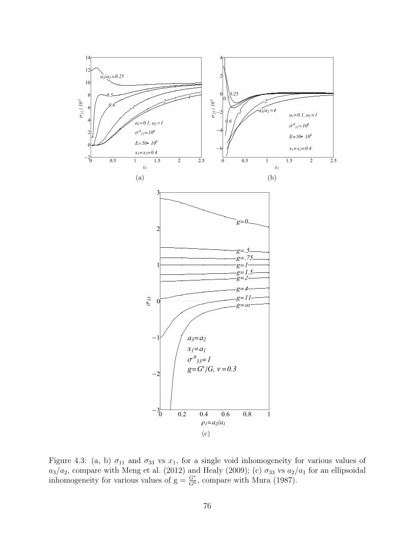
µ

µ µµ

µ

µ

µ

µ

µ

µ

µ

µ

µ

µ

µ

µ

µ

µ

µ

µ

µ

µ

µ

µ

a3êa2 =0.25

0.5

0.61

2

4

a1=0.1, a2 =1

s011=10

6

E=50µ109

x1=x2=0.4

0 0.5 1 1.5 2 2.5-2

0

2

4

6

8

10

12

14

x1

s11

ê10

5

(a)

0.25

0.5

0.6

1

2

a3êa2 =4

a1=0.1, a2 =1

s011=10

6

E=50µ109

x1=x2=0.4

0 0.5 1 1.5 2 2.5

-6

-4

-2

0

2

4

x1

s33

ê10

5

(b)

µ

µ

µ

µµ

µµ

µ

µµ

µ µ

µ µ µ µ µ µ

µ

µ

µµ

µ

µ µ µ µ µ µ

µ µ µ µ µ µ

µ µ µ µ µ µ

µ µ µµ

µ µ

µ

µ

µ

µ

µ

µ

g=¶

g=11

g=4

g=2g=1.5

g=1

g=.75

g=.5

g=0

a3=a2

x1=a1

s033=1

g=G*êG, n =0.3

0 0.2 0.4 0.6 0.8 1-3

-2

-1

0

1

2

3

r1=a2êa1

s33

(c)

Figure 4.3: (a, b) σ11 and σ33 vs x1, for a single void inhomogeneity for various values ofa3/a2, compare with Meng et al. (2012) and Healy (2009); (c) σ33 vs a2/a1 for an ellipsoidalinhomogeneity for various values of g = G∗

G0 , compare with Mura (1987).

76

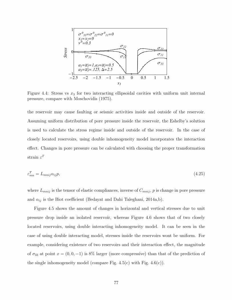
µ µµ

µ

µ

µ

µ

µ µ

µ µ µ µµ

µ

µµ µ

µ µ µ µµ

µ

µµ µ

s11

s11

s22s22

s33

s33

a1=a2=1,a2=a2=0.5

a3=a3=.125, D=2.5

s033=s

022=s

011=0

x1=x2=0

n0=0.3

-2.5 -2 -1.5 -1 -0.5 0 0.5 1 1.5

-1

0

1

x3

Str

ess

Figure 4.4: Stress vs x3 for two interacting ellipsoidal cavities with uniform unit internalpressure, compare with Moschovidis (1975).

the reservoir may cause faulting or seismic activities inside and outside of the reservoir.

Assuming uniform distribution of pore pressure inside the reservoir, the Eshelby’s solution

is used to calculate the stress regime inside and outside of the reservoir. In the case of

closely located reservoirs, using double inhomogeneity model incorporates the interaction

effect. Changes in pore pressure can be calculated with choosing the proper transformation

strain εT

εTmn = Lmnijαijp, (4.25)

where Lmnij is the tensor of elastic compliances, inverse of Cmnij, p is change in pore pressure

and αij is the Biot coefficient (Bedayat and Dahi Taleghani, 2014a,b).

Figure 4.5 shows the amount of changes in horizontal and vertical stresses due to unit

pressure drop inside an isolated reservoir, whereas Figure 4.6 shows that of two closely

located reservoirs, using double interacting inhomogeneity model. It can be seen in the

case of using double interacting model, stresses inside the reservoirs wont be uniform. For

example, considering existence of two reservoirs and their interaction effect, the magnitude

of σ33 at point x = (0, 0,−1) is 8% larger (more compressive) than that of the prediction of

the single inhomogeneity model (compare Fig. 4.5(c) with Fig. 4.6(c)).

77

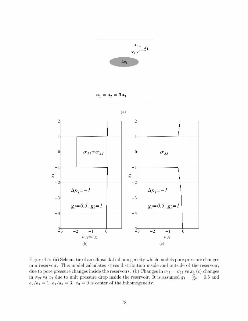
Δ𝑝1

𝐚𝟏 = 𝐚𝟐 = 𝟑𝐚𝟑

(a)

s11=s22

Dp1=-1

g1=0.5, g2=1

-3 -2 -1 0-5

-4

-3

-2

-1

0

1

2

s11=s22

x3

(b)

s33

Dp1=-1

g1=0.5, g2=1

-3 -2 -1 0-5

-4

-3

-2

-1

0

1

2

s33

x3

(c)

Figure 4.5: (a) Schematic of an ellipsoidal inhomogeneity which models pore pressure changesin a reservoir. This model calculates stress distribution inside and outside of the reservoir,due to pore pressure changes inside the reservoirs. (b) Changes in σ11 = σ22 vs x3 (c) changesin σ33 vs x3 due to unit pressure drop inside the reservoir. It is assumed g1 = G∗

G0 = 0.5 anda2/a1 = 1, a1/a3 = 3. x3 = 0 is center of the inhomogeneity.

78

Δ𝑝1

Δ𝑝2

𝐚𝟏 = 𝐚𝟐 = 𝟑𝐚𝟑

(a)

s11=s22

Dp1=Dp2=-1

g=0.5

-3 -2 -1 0-5

-4

-3

-2

-1

0

1

2

s11=s22

x3

(b)

s33

Dp1=Dp2=-1

g=0.5

0-1-2-3-5

-4

-3

-2

-1

0

1

2

s33

x3

(c)

Figure 4.6: (a) Schematic of two ellipsoidal inhomogeneities which models pore pressurechanges in two adjacent reservoirs. This model calculates stress distribution inside andoutside of two adjacent reservoir, due to pore pressure changes inside the reservoirs. (b)Changes in σ11 = σ22 vs x3 (c) changes in σ33 vs x3 due to unit pressure drop inside twoadjacent reservoirs. It is assumed g1 = g2 = G∗

G0 = 0.5 and a2/a1 = 1, a1/a3 = 3. x3 = 0 andx3 = −3 are centers of the two ellipsoidal inhomogeneities.

79

4.6 Conclusion

Determining the elastic fields inside and outside of inhomogeneities have many applica-

tions in the geoscience, material science, and biomechanics. For example, many geological

phenomena and structures like reservoirs, aquifers, intrusions, fault zones, caverns, dikes,

compaction bands, and other underground structures can be modeled as inhomogeneous in-

clusions, i.e. have different loading conditions and material properties rather than those of

the their surroundings.

We developed a Mathematica code to calculate the stress and strain fields inside and

outside of two interacting ellipsoidal inhomogeneities with arbitrary orientation with respect

to each other. This model can be used to predict pore pressure inside and outside of de-

pleting reservoirs. The results shows neglecting the interaction effect between the reservoirs,

predicts lower compressive stresses in depleted formations. Assuming same material prop-

erties for one of the inclusions and the surrounding matrix, this code can be also used for a

single inhomogeneity problem. This code is based on the solution provided by Moschovidis

and Mura (1975) for elastic and Bedayat and Dahi Taleghani (2014a) for poroelastic inho-

mogeneities. Considering interaction of the inhomogeneities, stress distribution inside the

inhomogeneities wont be uniform.

4.7 Supplementary data

Supplementary data associated with this article can be found in the author’s website.

4.8 Double inhomogeneity problem

In thissection, we present a short review of the solution developed by Moschovidis and Mura

(1975) to solve for double interacting inhomogeneities. Consider xi and xi are the local

coordinate systems taken at the center of Ω1 and Ω2, respectively. These coordinate systems

80

are related by

xi = aijxj + ci, (4.26)

xi = aji(xj − cj), (4.27)

where aij is the direction cosine of a vector connecting center of two inclusions, i.e. between

the xi axis and the xj axis, and ci is the xi coordinate of the origin of the coordinate system

attached to Ω2.

Let’s consider all the strain fields can be expressed by polynomial functions of coordinates.

For example, the applied strains before the disturbance (ε0ij(x) and ε0ij(x)) can be written

as

ε0ij(x) = Eij + Eijkxk + Eijklxkxl + · · · , (4.28)

ε0ij(x) = Eij + Eijkxk + Eijklxkxl + · · · . (4.29)

Similarly the equivalent eigenstrains (ε1∗ij (x) and ε2∗

ij (x)), and their corresponding strains can

be written as

ε1∗ij (x) = B1

ij +B1ijkxk +B1

ijklxkxl + · · · , (4.30)

ε2∗ij (x) = B2

ij +B2ijkxk +B2

ijklxkxl + · · · , (4.31)

and

ε1ij(x) = D1

ijkl(x)B1kl +D1

ijklq(x)B1klq +D1

ijklqr(x)B1klqr + · · · , (4.32)

81

ε2ij(x) = D2

ijkl(x)B2kl +D2

ijklq(x)B2klq +D2

ijklqr(x)B2klqr + · · · , (4.33)

where Eij... and Bij... are constant coefficients. Now Eqs. (4.7) and (4.8) can be expanded as

∆C1stmn

[D1mnij(0)B1

ij +D1mnijkl(0)B1

ijkl + · · ·]

+ amcanh[D2chij(0)B2

ij +D2chijk(0)B2

ijk

+D2chijkl(0)B2

ijkl + · · ·]− C0

stmnB1mnp = −∆C1

stmnEmnp

∆C1stmn

[ ∂

∂xpD1mnijk(0)B1

ijk + · · ·]

+ amcanhapf

[ ∂

∂xfD2chij(0)B2

ij +∂

∂xfD2chijk(0)B2

ijk

+∂

∂xfD2chijkl(0)B2

ijkl + · · ·]− C0

stmnB1mnp = −∆C1

stmnEmnp

etc.

in Ω1, (4.34)

and

∆C2stmn

[D2mnij(0)B2

ij +D2mnijkl(0)B2

ijkl + · · ·]

+ acmahn[D1chij(0)B1

ij +D1chijk(0)B1

ijk

+D1chijkl(0)B1

ijkl + · · ·]− C0

stmnB2mn = −∆C2

stmnEmn,

∆C2stmn

[ ∂

∂xpD2mnijk(0)B2

ijk + · · ·]

+ acmahnafp

[ ∂

∂xfD1chij(0)B1

ij +∂

∂xfD1chijk(0)B1

ijk

+∂

∂xfD1chijkl(0)B1

ijkl + · · ·]− C0

stmnB2mnp = −∆C2

stmnEmnp,

82

etc.

in Ω2. (4.35)

So that B1ij··· and B2

ij···, are the only unknowns in the system of Eqs. (4.34) and (4.35).

Obtaining these values, the strain at point x can be calculated from Eqs. (4.32) and (4.33)

εij(x) = ε1ij(x) + ε2

ij(x). (4.36)

4.9 Detailed formulation of Eshelby tensor D

According to Moschovidis (1975); Mura (1987), the derivative of I integrals are

Iij···k,p = Λij···kλ,p, (4.37)

Iij···k,pq = Λij···k[λ,pq − λ,pλ,qZ(1)IJ ···K ], (4.38)

Iij···k,pq = Λij···k

[λ,pqr − (λ,pqλ,r + λ,prλ,q + λ,qrλ,p)Z

(1)IJ ···K

+ λ,pλ,qλ,r[Z

(2)IJ ···K + (Z

(1)IJ ···K)2

]], (4.39)

etc.,

where

Λij···k =−2πa1a2a3

(a2i + λ)(a2

j + λ) · · · (a2k + λ)∆(λ)

, (4.40)

Z(n)ij···k =

1

(a2i + λ)n

+1

(a2j + λ)n

+ · · ·+ 1

(a2k + λ)n

83

+1

2

3∑m=1

1

(a2m + λ)n

, (4.41)

and the derivatives of λ are

λ,q =1

C1

Fq, (4.42)

λ,qp =1

C1

[Fq,p − λ,qC1,p], (4.43)

λ,qpr = − 1

C1

[λ,qpC1,r − Fq,pr + λ,qrC1,p + λ,qC1,pr], (4.44)

λ,qprt = − 1

C1

[λ,qprC1,t + λ,qptC1,r + λ,qpC1,rt − Fq,prt

+ λ,qrtC1,p + λ,qrC1,pt + λ,qtC1,pr + λ,qC1,prt], (4.45)

etc.,

where

Fq =2xq

(a2Q + λ)

, (4.46)

Fq,p =1

(a2Q + λ)

[2δqp − Fqλ,p], (4.47)

Fq,pr = − 1

(a2Q + λ)

[Fq,pλ,r + Fq,rλ,p + Fqλ,pr], (4.48)

Fq,prt = − 1

(a2Q + λ)

[Fq,prλ,t + Fq,ptλ,r + Fq,pλ,rt + Fq,rtλ,p

84

+ Fq,rtλ,p + Fq,rλ,pt + Fq,tλ,pr + Fqλ,prt], (4.49)

Cn =x2i

(a2I + λ)n+1

, (4.50)

C1,q =Fq

a2Q + λ

− 2C2λ,q, (4.51)

C2,q =Fq

(a2Q + λ)2

− 3C3λ,q, (4.52)

C1,qp =1

a2Q + λ

[Fq,p −

Fqa2Q + λ

λ,p

]− 2[C2,pλ,q + C2λ,qp], (4.53)

C2,qp =2δqp

(a2Q + λ)3

− 6xq(a2Q + λ)4

λ,p −6xp

(a2P + λ)4

λ,q

+ 12C4λ,qλ,p − 3C3λ,qp, (4.54)

C1,qpt = − 1

(a2Q + λ)2

[Fq,p −

Fqa2Q + λ

λ,p

]λ,t

+1

a2Q + λ

[Fq,pt −

Fq,ta2Q + λ

λ,p −Fq

a2Q + λ

λ,pt +Fq

(a2Q + λ)2

λ,pλ,t

]

− 2[C2,ptλ,q + C2,pλ,qt + C2,tλ,qp + C2λ,qpt], (4.55)

etc.

Similarly, V integrals and their derivative can be written as

V =1

2[I − xrxrIR], (4.56)

85

Vi =1

2[Ii − xrxrIRi], (4.57)

Vij =1

2[Iij − xrxrIRij], (4.58)

etc.,

and

Vij···k,p = −xpIPij···k, (4.59)

Vij···k,pq = −[δpqIPij···k + xpIPij···k,q], (4.60)

Vij···k,pqr = −[δpqIPij···k,r + δprIPij···k,q + xpIPij···k,qr], (4.61)

etc.,

So that we get the equations for φ, ψ and their derivatives as

φ = V, (4.62)

φn = a2NxnVN , (4.63)

φmn = a2M

[xmxna

2NVMN

+1

4δmn[V − xrxrVR − a2

M(VM − xrxrVRM)]], (4.64)

86

φ,ij = −δijII − xiII,J (4.65)

φn,i = a2N(δinVN + xnVN,i), (4.66)

φn,ij = a2N(δinVN,j + δjnVN,i + xnVN,ij), (4.67)

and

ψ,ijkl =− δijδkl[IK(λ)− a2IIIK(λ)]− (δikδjl + δjkδil)[IJ(λ)− a2

IIIJ(λ)]

− δijxk[IK(λ)− a2IIIK(λ)],l − (δikxj + δjkxi)[IJ(λ)− a2

IIIJ(λ)],l

− (δilxj + δjlxi)[IJ(λ)− a2IIIJ(λ)],k − xixj[IJ(λ)− a2

IIIJ(λ)],kl (4.68)

4.10 References

Bedayat, H., Dahi Taleghani, A., 2013. The equivalent inclusion method for poroelasticityproblems, in: Poromechanics V, American Society of Civil Engineers, Reston, VA. pp.1279–1288. doi:10.1061/9780784412992.153.

Bedayat, H., Dahi Taleghani, A., 2014a. Interacting double poroelastic inclusions. Mechanicsof Materials 69, 204–212. doi:10.1016/j.mechmat.2013.10.006.

Bedayat, H., Dahi Taleghani, A., 2014b. On the inhomogeneous anisotropic poroelasticinclusions. Mechanics of Materials (Under Review) .

Chen, Z.R., 2011. Poroelastic model for induced stresses and deformations in hydrocar-bon and geothermal reservoirs. Journal of Petroleum Science and Engineering 80, 41–52.doi:10.1016/j.petrol.2011.10.004.

87

Dyson, F., 1891. The potentials of ellipsoids of variable densities. Quart. J. Pure Appl. Math25, 259–288.

Eshelby, J.D., 1957. The determination of the elastic field of an ellipsoidal inclusion, andrelated problems. Proceedings of the Royal Society A: Mathematical, Physical and Engi-neering Sciences 241, 376–396. doi:10.1098/rspa.1957.0133.

Eshelby, J.D., 1959. The elastic field outside an ellipsoidal inclusion, in: Proceedings of theRoyal Society of London. Series A, Mathematical and Physical, pp. 561–569.

Ferrers, N., 1877. On the potentials of ellipsoids, ellipsoidal shells, elliptic laminae andelliptic rings of variable densities. QJ Pure Appl. Math 14, 1–22.

Healy, D., 2009. Elastic field in 3D due to a spheroidal inclusionMATLAB code for Eshelby’ssolution. Computers & Geosciences 35, 2170–2173. doi:10.1016/j.cageo.2008.11.012.

Honein, E., Honein, T., Herrmann, G., 1992. On two circular inclusions in harmonic prob-lems. Quarterly of applied mathematics 50, 479–499.

Horii, H., Nemat-Nasser, S., 1985. Elastic fields of interacting inhomogeneities. InternationalJournal of Solids and Structures 21, 731–745. doi:10.1016/0020-7683(85)90076-9.

Kachanov, M.L., Laures, J.P., 1989. Three-dimensional problems of strongly interactingarbitrarily located penny-shaped cracks. International Journal of Fracture 41, 289–313.doi:10.1007/BF00018861.

Li, S., Sauer, R.a., Wang, G., 2007. The Eshelby tensors in a finite pherical domain-Part I:theoretical formulations. Journal of Applied Mechanics 74, 770. doi:10.1115/1.2711227.

Meng, C., Heltsley, W., Pollard, D.D., 2012. Evaluation of the Eshelby solution for theellipsoidal inclusion and heterogeneity. Computers & Geosciences 40, 40–48. doi:10.1016/j.cageo.2011.07.008.

Moschovidis, Z.A., 1975. Two ellipsoidal inhomogeneities and related problems treated bythe equivalent inclusion method. Ph.D. thesis. Northwestern University, Evanston.

88

Moschovidis, Z.A., Mura, T., 1975. Two-ellipsoidal inhomogeneities by the Equivalent In-clusion Method. Journal of Applied Mechanics 42, 847. doi:10.1115/1.3423718.

Mura, T., 1987. Micromechanics of defects in solids. Martinus Nijhoff Publishers.

Rudnicki, J.W., 2002a. Alteration of regional stress by reservoirs and other inhomo- geneities:Stabilizing or destabilizing?, in: Vouille, G., Berest, P. (Eds.), Proc. 9th Int. Congr. RockMechanics,Vol. 3, Paris, Aug. 25-29, 1999, Paris, France. pp. 1629– 1637.

Rudnicki, J.W., 2002b. Eshelby transformations, pore pressure and fluid mass changes, andsubsidence, in: Poromechanics II, Proc. 2nd Biot Conference on Poromechanics, Grenoble,France.

Rudnicki, J.W., 2011. Eshelbys technique for analyzing inhomogeneities in geomechanics,in: Leroy, Y.M., Lehner, F.K. (Eds.), Mechanics of Crustal Rocks. Springer Vienna, pp.43–72. doi:10.1007/978-3-7091-0939-7.

Shodja, H.M., Ojaghnezhad, F., 2007. A general unified treatment of lamellar inhomo-geneities. Engineering Fracture Mechanics 74, 1499–1510. doi:10.1016/j.engfracmech.2006.08.016.

Shodja, H.M., Rad, I., Soheilifard, R., 2003. Interacting cracks and ellipsoidal inhomo-geneities by the equivalent inclusion method. Journal of the Mechanics and Physics ofSolids 51, 945–960. doi:10.1016/S0022-5096(02)00106-0.

Shojaei, A., Li, G., 2013. Viscoplasticity analysis of semicrystalline polymers: A multiscaleapproach within micromechanics framework. International Journal of Plasticity 42, 31–49.doi:10.1016/j.ijplas.2012.09.014.

Soltanzadeh, H., Hawkes, C.D., 2012. Evaluation of caprock integrity during pore pressurechange using a probabilistic implementation of a closed-form poroelastic model. Interna-tional Journal of Greenhouse Gas Control 7, 30–38. doi:10.1016/j.ijggc.2011.10.006.

Soltanzadeh, H., Hawkes, C.D., Sharma, J.S., 2007. poroelastic model for production-and injection-induced stresses in reservoirs with elastic properties different from the sur-rounding rock. International Journal of Geomechanics 7, 353–361. doi:10.1061/(ASCE)1532-3641(2007)7:5(353).

89

Walsh, J.B., 2002. Subsidence above a planar reservoir. Journal of Geophysical Research107, 2202. doi:10.1029/2001JB000606.

Zhou, K., Hoh, H.J., Wang, X., Keer, L.M., Pang, J.H., Song, B., Wang, Q.J., 2013. Areview of recent works on inclusions. Mechanics of Materials 60, 144–158. doi:10.1016/j.mechmat.2013.01.005.

Zhou, K., Keer, L.M., Jane Wang, Q., Ai, X., Sawamiphakdi, K., Glaws, P., Paire, M., Che,F., 2012. Interaction of multiple inhomogeneous inclusions beneath a surface. ComputerMethods in Applied Mechanics and Engineering 217-220, 25–33. doi:10.1016/j.cma.2012.01.006.

Zou, W., He, Q., Huang, M., Zheng, Q., 2010. Eshelby’s problem of non-elliptical inclusions.Journal of the Mechanics and Physics of Solids 58, 346–372. doi:10.1016/j.jmps.2009.11.008.

90

Chapter 5Drainage of Poroelastic Fractures andIts Implications on the Performance ofNaturally Fractured Reservoirs 1

Large volumes of natural gas and oil are stored in low-permeability fractured reservoirs

around the world. Extensive field and lab measurements have revealed presence of natural

fracture in different scales and their fractal distributions. The log normal distribution of frac-

tures length and width and their consistency throughout the formation is well documented

for different basins in the literature; but the mechanical implications and the potential roles

of these distributions on the fluid flow behavior in the rock is not yet studied. This paper

provides poroelastic analysis for a single micro-fracture subject to fluid withdrawal (pro-

duction) through the fracture. Formation is assumed to be a low permeable poroelastic

medium. The main drive behind studying this problem was the fact that core flooding mea-

surements in laboratory studies indicate that permeability of tight formations rock samples

is in the order of nanodarcy, however the rate of production from the stimulated and even

non-stimulated wells are leading us to average values for shale permeability, which are orders

of magnitudes higher than the permeability measured in the lab. In this paper, we are trying

to verify the role of natural fractures and their poroelastic properties to explain discrepancy

in the measured permeability using different methods. To achieve this goal, we provide an

1Bedayat, H., & Dahi Taleghani, A., 2012. Drainage of Poroelastic Fractures and Its Implications onthe Performance of Naturally Fractured Reservoirs. In 46th US Rock Mechanics/Geomechanics Symposium.Chicago, IL, USA. ARMA-2012-562.

91

analytical solution for fracture volume changes due to fluid withdrawal (production). The

roles of differential in-situ stress and formation pressure in determining the crack volume

changes were found to be significant. The results could be used to relate the significant

reduction in production from some of the shale gas wells to the closure of microfractures

or even larger non-propped fractures. In general having the knowledge of mechanical and

hydraulic behavior of natural micro-fractures in low permeability reservoirs could be a key to

predict the production decline in these formations and provide insight to more sophisticated

stimulation techniques in future.

5.1 Introduction

The scarce amount of conventional hydrocarbon reservoirs and the increase of fuel consump-

tion all over the world have made production from unconventional hydrocarbon resources

inevitable. Large volumes of natural gas and oil are stored in low-permeability fractured

reservoirs around the world. Tight gas sandstones are part of what is known as unconven-

tional gas, which also includes coal bed methane, shale gas and natural gas hydrates. Based

on the U.S. Gas Policy Act of 1978, if the in-situ gas permeability of a reservoir is equal to

or less than 0.1 md, it is designated as a tight gas formation (Kazemi, 1982). Independent

of this definition, natural fractures are extremely important to unconventional gas reservoirs

(Aguilera, 2008), because without fractures, it is not possible to recover hydrocarbons from

these reservoirs.

Because of the low permeability of these formations and the low conductivity of the

natural fracture networks, stimulation techniques such as hydraulic fracturing are neces-

sary to make economic production possible. The low conductivity of the natural fracture

system could be caused by occluding cements that precipitated during the diagenesis pro-

cess (Laubach, 2003; Gale et al., 2007; Dahi Taleghani, 2011). For instance, almost all the

cores recovered from the Forth Worth basin in the Barnett Shale contain cemented natural

92

fractures (Gale et al., 2007). In the Delaware basin, few partially cemented fractures are

identified in the cores, and the rest of the fractures are sealed by cements (Ali, 2009).

The fact that natural fractures might be sealed by cements does not mean that they

can be ignored while designing well completion processes. Cemented natural fractures can

still act as weak paths for fracture growth (Dahi Taleghani and Olson, 2011). One common

observation during hydraulic fracturing in naturally fractured reservoirs is a high leakoff

rate during the treatment. In some cases, fluid leakoff in these reservoirs are reported to

be as high as fifty times larger than the fluid leakoff in non-fractured reservoirs. This issue

becomes more interesting with the knowledge that in non-fractured reservoirs, the leakoff

rate depends on formation permeability, net treatment pressure and fracture fluid parameters

(Valko and Economides, 1995); however field observation during hydraulic fracturing in

fractured reservoirs shows that, surprisingly, leakoff in these reservoirs primarily depends on

net treatment pressure and fracture fluid parameters but not formation permeability (Britt

et al., 1994; Barree, 1998). All these observations confirms the opening of natural fractures

during hydraulic fracturing treatments.

Fractures are discrete discontinuity in a rock mass that developed as a response to stress,

i.e., brittle failure. They are a universal element in sedimentary rocks. Furthermore, except

some extremely ductile rocks such as salt or certain shale, all rocks in all depths can be

considered as fractured media. In fractured rocks, fractures are responsible for the main part

of the permeability and they affect the overall mechanical behavior of the rock mass (Britt

et al., 1994; Gillespie et al., 1993). Fractures exist on a wide range of scales from microns

to hundreds of kilometers, and it is known that throughout this scale range they have a

significant effect on processes in the Earth’s crust including fluid flow and rock strength.

Early work was spread though a wide range of scales from core through outcrop to aerial

photographs and satellite image scales. More recently, the manner in which fracture system

properties at different scales relate to each other, i.e., their scaling attributes, has received

increasing attention motivated by the promise of statistical prediction that scaling laws offer

93

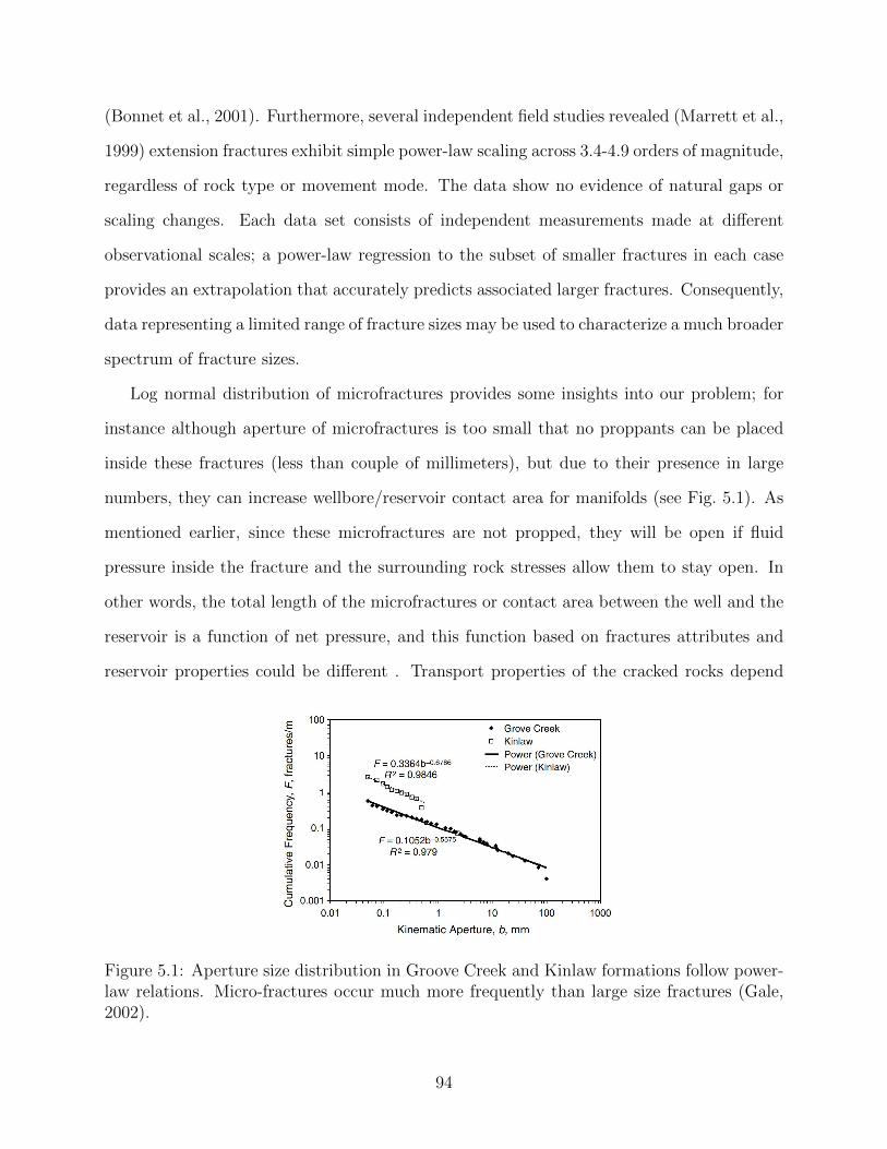
(Bonnet et al., 2001). Furthermore, several independent field studies revealed (Marrett et al.,

1999) extension fractures exhibit simple power-law scaling across 3.4-4.9 orders of magnitude,

regardless of rock type or movement mode. The data show no evidence of natural gaps or

scaling changes. Each data set consists of independent measurements made at different

observational scales; a power-law regression to the subset of smaller fractures in each case

provides an extrapolation that accurately predicts associated larger fractures. Consequently,

data representing a limited range of fracture sizes may be used to characterize a much broader

spectrum of fracture sizes.

Log normal distribution of microfractures provides some insights into our problem; for

instance although aperture of microfractures is too small that no proppants can be placed

inside these fractures (less than couple of millimeters), but due to their presence in large

numbers, they can increase wellbore/reservoir contact area for manifolds (see Fig. 5.1). As

mentioned earlier, since these microfractures are not propped, they will be open if fluid

pressure inside the fracture and the surrounding rock stresses allow them to stay open. In

other words, the total length of the microfractures or contact area between the well and the

reservoir is a function of net pressure, and this function based on fractures attributes and

reservoir properties could be different . Transport properties of the cracked rocks depend

Figure 5.1: Aperture size distribution in Groove Creek and Kinlaw formations follow power-law relations. Micro-fractures occur much more frequently than large size fractures (Gale,2002).

94

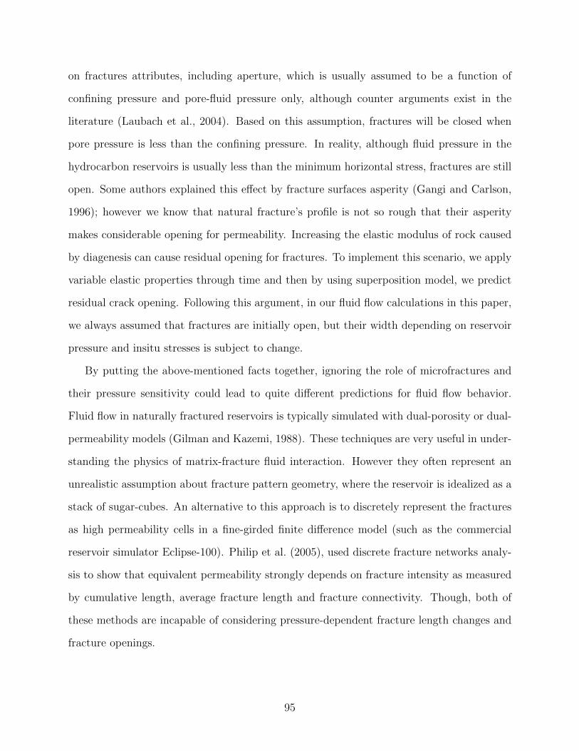
on fractures attributes, including aperture, which is usually assumed to be a function of

confining pressure and pore-fluid pressure only, although counter arguments exist in the

literature (Laubach et al., 2004). Based on this assumption, fractures will be closed when

pore pressure is less than the confining pressure. In reality, although fluid pressure in the

hydrocarbon reservoirs is usually less than the minimum horizontal stress, fractures are still

open. Some authors explained this effect by fracture surfaces asperity (Gangi and Carlson,

1996); however we know that natural fracture’s profile is not so rough that their asperity

makes considerable opening for permeability. Increasing the elastic modulus of rock caused

by diagenesis can cause residual opening for fractures. To implement this scenario, we apply

variable elastic properties through time and then by using superposition model, we predict

residual crack opening. Following this argument, in our fluid flow calculations in this paper,

we always assumed that fractures are initially open, but their width depending on reservoir

pressure and insitu stresses is subject to change.

By putting the above-mentioned facts together, ignoring the role of microfractures and

their pressure sensitivity could lead to quite different predictions for fluid flow behavior.

Fluid flow in naturally fractured reservoirs is typically simulated with dual-porosity or dual-

permeability models (Gilman and Kazemi, 1988). These techniques are very useful in under-

standing the physics of matrix-fracture fluid interaction. However they often represent an

unrealistic assumption about fracture pattern geometry, where the reservoir is idealized as a

stack of sugar-cubes. An alternative to this approach is to discretely represent the fractures

as high permeability cells in a fine-girded finite difference model (such as the commercial

reservoir simulator Eclipse-100). Philip et al. (2005), used discrete fracture networks analy-

sis to show that equivalent permeability strongly depends on fracture intensity as measured

by cumulative length, average fracture length and fracture connectivity. Though, both of

these methods are incapable of considering pressure-dependent fracture length changes and

fracture openings.

95

Besides the above-discussed field observations, core measurements in laboratory indicate

that permeability of rock samples recovered from NFRs (for example shale reservoirs) is

in the order of nanodarcy, however the rate of production from the stimulated and even

non-stimulated wells are leading us to average values of much higher probabilities. Some

researchers have tried to relate this phenomenon to the presence of micro-scale natural frac-

tures in the formation David and Ravalec-Dupin (2007). Hence in this paper, we try to verify

the role of natural fractures and their poroelastic properties on production. Some recovered

cores from the hydraulic fractures have confirmed the presence of large number of small size

natural fractures on the surface of induced hydraulic fractures. However they are too small

to contain proppants, but they can increase reservoir/fracture contact surface tremendously.

On the other hand since these fractures are not propped, their opening and consequently

their permeability will be a function of pressure and poroelastic properties of the rock. In

this paper, we provide analytical solution for fracture volume changes due to fluid withdrawal

(production) and similarly fluid injection. Producing and injecting fluids change pore pres-

sure and rock stresses. The fluid flow induced stresses causes deformations in the rock that

changes fracture apertures (Heffer et al., 1995). Thus change in the hydraulic conductivity of

fractures and consequently overall permeability could directly affect production (Koutsabe-

loulis et al., 1994; Heffer et al., 1995). Therefore, having knowledge of mechanical as well

as hydraulic behavior of natural microfractures in low permeability reservoirs is a key for

understanding and predicting the reservoir behavior during production.

As the first step to tackle this problem, we try to demonstrate the behavior of a single

microfractures to pressure and stress changes in the formation due to the production. This

work provides poroelastic analysis of a stationary micro-fracture due to fluid production

through the fracture. Atkinson and Craster (1991); Craster and Atkinson (1994) solved this

problem analytically for a semi-infinite growing hydraulic fracture using Wiener-Hopf and

integral transform method. However, these methods are not applicable for finite size sta-

tionary fractures, and their asymptotic solution could not predict fracture behavior between

96

long-term and short-term. Almost at the same time, Detournay and Cheng (1991) tried to

solve poroelasticity equations to calculate leak-off volume in a stationary finite-size hydraulic

fracture.

5.2 Statement of the Problem & Assumptions

In this paper, we are trying to investigate the poroelastic behavior of a single microfracture.

Rather than considering a population of microfractures, we start with poroelastic analysis for

a single fracture with the length of 2L in an infinite homogeneous and isotropic poroelastic

medium and show how fracture length and its depth or more precisely the magnitude of

in-situ stress normal to the fracture plane may affect fracture volume (see Fig. 5.2). Hence,

fracture is assumed to keep its constant length, fracture volume changes imply fracture

width, i.e., permeability changes. The formation rock is assumed to be fully saturated with

a Newtonian fluid with viscosity, µ. The mechanical behavior of the rock is assumed to

be linear elastic, so we can limit our analysis to linear fracture mechanics (Detournay and

Cheng, 1991). The fracture is assumed to be drained into a connected borehole or through

a network of fractures. Thus, the initial fracture pressure is presumed to be equal to the

formation pressure, i.e. pf = pr = p0. Since, the borehole fluid has lower pressure than

formation fluid and fracture has higher permeability than the formation matrix, formation

fluid begins to flow into the borehole. Due to production, we expect instantaneous fluid

pressure drop inside the fracture. Thus the fractures pore pressure at time t = t0+

is equal

to pbh and it will remain constant for a long time, t > 0 . To avoid further complications,

we assume that fracture remains in the plane, so we can use plain strain condition for stress

analysis. Figure 3 demonstrates the schematic view of the problem.

97

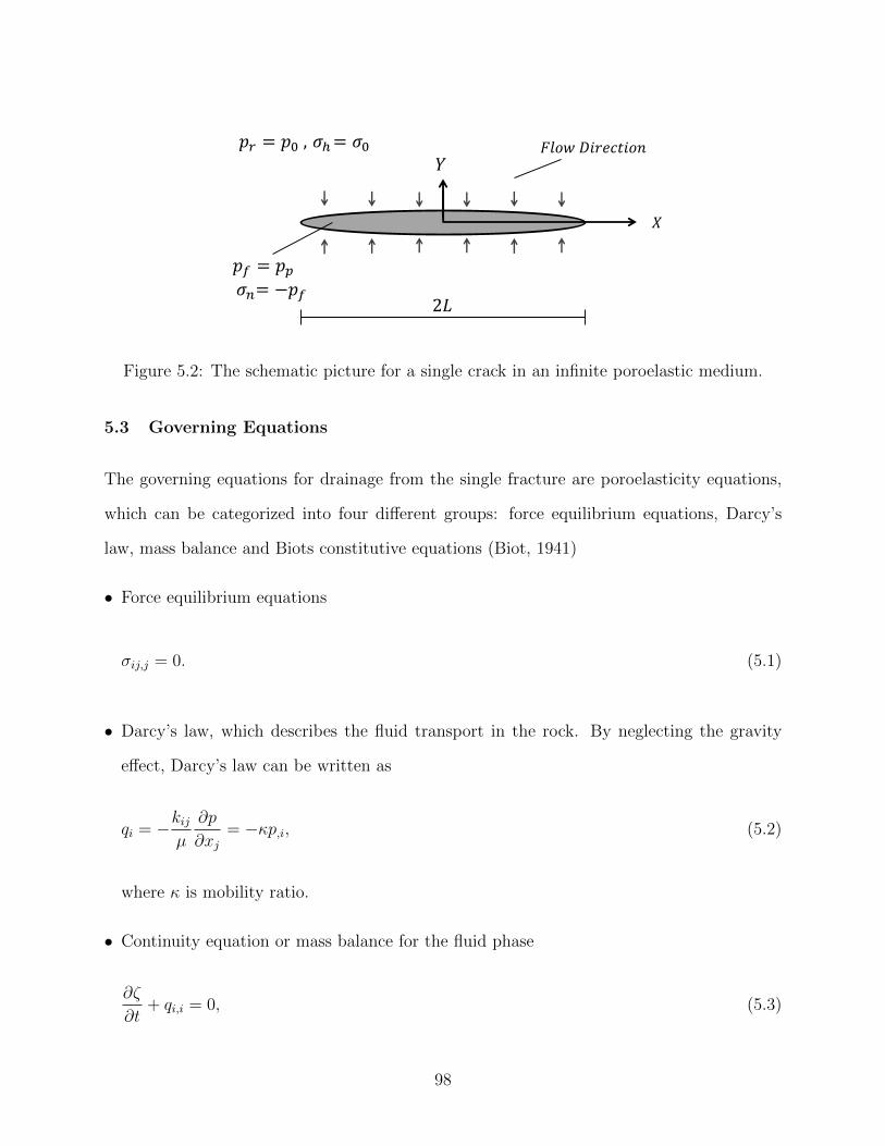
𝑋

𝑌

𝑝𝑟 = 𝑝0 , 𝜎ℎ= 𝜎0

2𝐿

𝑝𝑓 = 𝑝𝑝𝜎𝑛= −𝑝𝑓

𝐹𝑙𝑜𝑤 𝐷𝑖𝑟𝑒𝑐𝑡𝑖𝑜𝑛

Figure 5.2: The schematic picture for a single crack in an infinite poroelastic medium.

5.3 Governing Equations

The governing equations for drainage from the single fracture are poroelasticity equations,

which can be categorized into four different groups: force equilibrium equations, Darcy’s

law, mass balance and Biots constitutive equations (Biot, 1941)

• Force equilibrium equations

σij,j = 0. (5.1)

• Darcy’s law, which describes the fluid transport in the rock. By neglecting the gravity

effect, Darcy’s law can be written as

qi = −kijµ

∂p

∂xj= −κp,i, (5.2)

where κ is mobility ratio.

• Continuity equation or mass balance for the fluid phase

∂ζ

∂t+ qi,i = 0, (5.3)

98

where ζ is incremental fluid content and it is defined as

ζ =∂mf

ρf0. (5.4)

• Biot’s poroelastic constitutive equations, which describe the constitutive equations for a

fluid-filled porous media. It assumes linear and reversible relationship between stresses

(σij, p) on one side and kinematics i.e. strains and fluid content (εij, ζ) on the other side,

2Gεij = σij − νσkkδij + α(1− 2ν)pδij, (5.5)

2Gζ = α(1− 2ν)σkk +α2(1− 2ν)2

νu − νp, (5.6)

where δij is the Kronecker delta (δij = 1 for i = j, and δij = 0 for i 6= j) and index

notation convention has been used; so i and j indices take values 1 and 2.

Our approach for solving this problem is essentially inspired by modal decomposition and

superposition method previously developed and used to solve several poroelasticity problems

like sudden pressurization of a borehole. Detournay and Cheng (1991) solved the stress

and pressure distribution for a stationary hydraulic fracture using this method too. In

hydraulic fracturing, fluid is injected into the fracture to induce further tensile stresses

and consequently cracking the formation rock. Injection increases fluid pressure inside the

fracture as well as pore pressure in the fracture vicinity. Pressure difference between inside

and outside of the crack, pushes fluid to move from the fracture into the formation (pf−pr >

0). However, the situation for producing fluids from the fracture is almost vice versa. Fluid

moves from the formation rock with higher pore pressure to fractures with lower pressure

(pf − pr < 0). The same governing equations still applies to this problem but with different

boundary conditions and initial conditions due to the change of the fluid flow direction. We

assume the stress intensity factor at the tip of the receding fracture is equal to zero.

99

Following discussions in the previous section, we assume that at the initial time (t = 0),

fractures are open. Pre-existing fractures might be open due to existence of driving pore

pressure larger than minimum effective horizontal stress, thermal stress, residual in-situ stress

or the effect of a near major fault (Engelder and Lacazette, 1990; Olson et al., 2009; Gale

et al., 2010). At the initial time, the condition is undrained and fracture volume in undrained

condition can be calculated using linear elastic fracture mechanics solution Sneddon (1946).

For a unit uniform stress applied on the fracture wall, the initial fracture opening is given

by

Dn(x) = −2(1− νu)G

√L2 − x2 (5.7)

and initial fracture volume may also be derived by integration of Eq. (5.7).

Multiplying the magnitude of the net fluid pressure inside the fracture by the initial

fracture volume for unit pressure gives the volume of the fracture for a given reservoir

pressure, i.e.

V initialf =

πL2(1− νu)G

pd, (5.8)

where, pd is the net pressure, and it is defined as the difference between fluid pressure inside

the fracture and in-situ minimum stress.

5.3.1 Mode decomposition

The normal traction and pore pressure along the fracture surface is equal to the fluid pres-

sure inside the fracture (σn = −pf , pp = pf ). Therefore, the response of the crack can be

decomposed into two fundamental problems: (1) a step change in stress while maintaining

constant pore pressure, (2) a step change in pore pressure while maintaining constant stress.

The fracture response in general condition is the linear combination of each of these modes.

In the calculations of the fundamental solutions, it has been assumed that the pore pressure

100

inside the fracture drops immediately and it will not change by time. However for the prob-

lems with time varying pressure, Duhamels theorem can be simply utilized generate solution

for arbitrary pressure changes in time.

The boundary conditions for two fundamental loading modes are provided below:

• Mode I

σn(x, t) = −1

p(x, t) = 0

(5.9)

• Mode II

σn(x, t) = 0

p(x, t) = −1

(5.10)

Let F1 and F2 be the fundamental solutions for mode I and mode II, respectively. In the

presence of compressive in-situ stresses (σ0), and reservoir initial pore pressure (pr = p0),

the solution for fracture volume or fracture width may be given as

Fp = (pf − σ0)F1 + (pf − p0)F2. (5.11)

The reader may notice that to simplify the problem, mode I and mode II are representing

the unit excess fluid pressure inside the fracture. However the fluid pressure inside the

fracture is less than fluid pressure inside the medium. Hence, pp − pf would be less than

zero for a fluid producing fracture. We always assumed that the formation pore pressure is

greater than or equal to the wellbore/fracture pressure. This difference in pressure causes the

fluid to migrate from the reservoir to the micro-fracture. Note micro-fractures are assumed

to have hydraulic connectivity with the wellbore, directly or by means of other fractures.

101

5.3.2 Fundamental solutions

Initial response for mode I loading is mainly due to the instantaneous change of fracture

traction, so the solution is similar to elasticity solution except the Poissons ratio which is

undrained, i.e.

V 1c (t = 0+) =

πL2(1− νu)G

. (5.12)

This increase in volume causes generation of pore pressure near the fracture wall. Hence,

liquid flows to the fracture after generation of excessive pore pressure. The amount of liquid

exchange volume may be calculated by integrating one dimensional flow flux perpendicular

to fracture length over the time, multiplying by circumference of fracture and the amount

of generated pore pressure. One dimensional flow perpendicular to fracture opening is a

valid assumption for a short time after pressure generation in the vicinity of the fracture.

Therefore the amount of liquid exchange volume for mode I is

V 1ex(t) = −8αL2(1− 2ν)(1− νu)

G√π(1− ν)

√ct

L2for

ct

L2 1, (5.13)

where c is the diffusivity coefficient given by

c =2κG(1− ν)(νu − ν)

α2(1− 2ν)2(1− νu). (5.14)

The amount of fluid which flows inside the fracture plus its initial volume is equal to total

fracture volume change. Therefore, the short-term response will be mainly driven by summa-

tion of instantaneous volume change and product of the amount of instantaneous generated

pore pressure field by volume change due to existence of unit pure pore pressure inside the

fracture.

V 1c (t) =

πL2(1− νu)G

+ (16L2νu − ν)(1− νu)

G√π(1− ν)

√ct

L2for

ct

L2 1. (5.15)

102

As time evolves to infinity, the fracture volume reaches to the elasticity solution

V 1c (∞) =

πL2(1− ν)

G, (5.16)

which is exactly same as Eq. (5.13), unless the undrained Poisson’s ratio is substituted with

the drained Poisson’s ratio.

Also as time goes to infinity, fluid exchange volume for mode I reaches to

V 1ex(∞) = −απL

2(1− 2ν)

2G. (5.17)

For mode II, using the principal of virtual work (Cleary, 1977), and calculated fluid exchange

volume for mode I (which is equal to fracture volume change in mode II), the volume of

the fracture right after application of mode II loading is given by

V 2c (t) = −8αL2(1− 2ν)(1− νu)

G√π(1− ν)

√ct

L2for

ct

L2 1, (5.18)

which at times equal to infinity reaches to

V 2c (∞) = −απL

2(1− 2ν)

2G. (5.19)

For a short time and unit excess pore pressure, similar to Eq. (5.14), fluid exchange volume

is equal to integral of one dimensional flow flux perpendicular to fracture opening over the

time multiplied by fracture circumference. Thus, fluid exchange for mode II will be

V 2c (t) =

8κL2

c√π

√ct

L2for

ct

L2 1. (5.20)

As times evolves to infinity, the fluid exchange volume may be estimated with leak off volume

from a circular hole with the same circumference, with unit rise constant pressure loading

103

on its diameter (Carslaw and Jaeger, 1959)

V 2ex(t) =

8κ

π

∫ ∞ε

1− e−cu2t

cu3[J20 (2L

πu) + Y 2

0 (2Lπu)]

du forct

L2 1, (5.21)

where J0 and Y0 are zero order Bessel functions of first and second kinds, respectively. Finally,

using the superposition principle and substituting Eqs. (5.15) to (5.19) in Eq. (5.11), the

final volume change of the fracture under the both modes loading is given by

Vc(t) = (pp − σ0)V 1c (t) + (pp − p0)V 2

c (t). (5.22)

The transitional response of the fracture between these two asymptotic conditions (t = 0, t =

∞), should be calculated numerically with boundary element methods or finite element

methods (Vandamme et al., 1989; Ghassemi and Zhang, 2006). The volume of the fracture

at any time is equal to sum of initial volume and change of the volume.

5.4 Results and Discussions

Through some examples, we investigate micro-fractures volume changes versus time due

to formation pressure changes. Using Eq. (5.22) long-term and short-term solutions for

fracture volume changes are calculated and for the transition between mentioned asymptotic

conditions, exponential regression has been used which agrees with approximate displacement

discontinuity solutions used in other references (Detournay and Cheng, 1991; Vandamme

et al., 1989).

Fractures are assumed to be open during production. The term (pp−σ0) might be positive

or negative depending on the magnitude of in-situ stresses. Thus, the resultant changes in

the fracture volume caused by mode I might be positive or negative. Therefore, one might

expect that in different tectonic regimes and wellbore pressure condition, effective stresses

may increase or decrease the total fracture volume i.e. overall permeability.

104

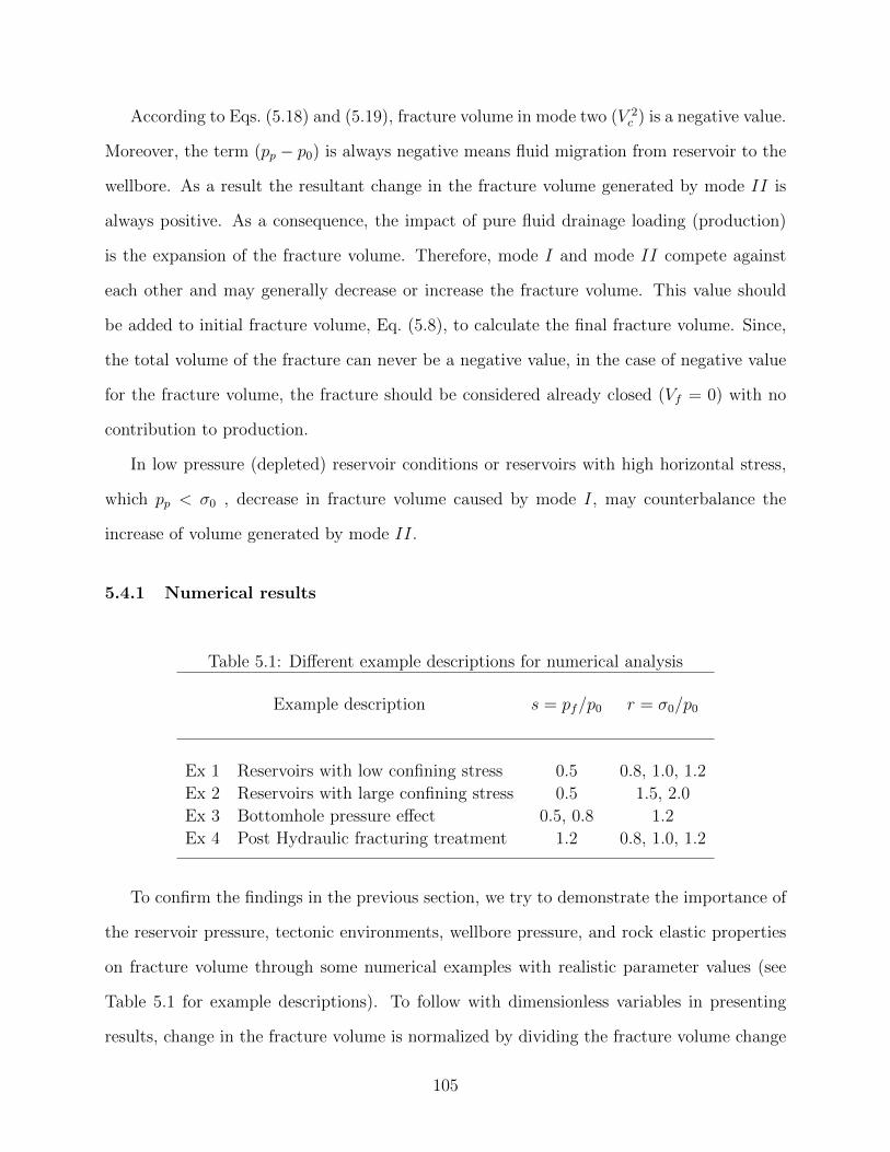
According to Eqs. (5.18) and (5.19), fracture volume in mode two (V 2c ) is a negative value.

Moreover, the term (pp − p0) is always negative means fluid migration from reservoir to the

wellbore. As a result the resultant change in the fracture volume generated by mode II is

always positive. As a consequence, the impact of pure fluid drainage loading (production)

is the expansion of the fracture volume. Therefore, mode I and mode II compete against

each other and may generally decrease or increase the fracture volume. This value should

be added to initial fracture volume, Eq. (5.8), to calculate the final fracture volume. Since,

the total volume of the fracture can never be a negative value, in the case of negative value

for the fracture volume, the fracture should be considered already closed (Vf = 0) with no

contribution to production.

In low pressure (depleted) reservoir conditions or reservoirs with high horizontal stress,

which pp < σ0 , decrease in fracture volume caused by mode I, may counterbalance the

increase of volume generated by mode II.

5.4.1 Numerical results

Table 5.1: Different example descriptions for numerical analysis

Example description s = pf/p0 r = σ0/p0

Ex 1 Reservoirs with low confining stress 0.5 0.8, 1.0, 1.2

Ex 2 Reservoirs with large confining stress 0.5 1.5, 2.0

Ex 3 Bottomhole pressure effect 0.5, 0.8 1.2

Ex 4 Post Hydraulic fracturing treatment 1.2 0.8, 1.0, 1.2

To confirm the findings in the previous section, we try to demonstrate the importance of

the reservoir pressure, tectonic environments, wellbore pressure, and rock elastic properties

on fracture volume through some numerical examples with realistic parameter values (see

Table 5.1 for example descriptions). To follow with dimensionless variables in presenting

results, change in the fracture volume is normalized by dividing the fracture volume change

105

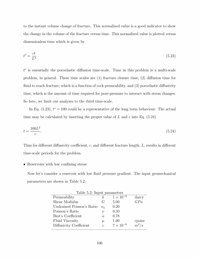
to the instant volume change of fracture. This normalized value is a good indicator to show

the change in the volume of the fracture versus time. This normalized value is plotted versus

dimensionless time which is given by

t∗ =ct

L2. (5.23)

t∗ is essentially the poroelastic diffusion time-scale. Time in this problem is a multi-scale

problem, in general. These time scales are (1) fracture closure time, (2) diffusion time for

fluid to reach fracture, which is a function of rock permeability, and (3) poroelastic diffusivity

time, which is the amount of time required for pore-pressure to interact with stress changes.

So here, we limit our analyses to the third time-scale.

In Eq. (5.23), t∗ = 100 could be a representative of the long term behaviour. The actual

time may be calculated by inserting the proper value of L and c into Eq. (5.24)

t =100L2

c. (5.24)

Thus for different diffusivity coefficient, c, and different fracture length, L, results in different

time-scale periods for the problem.

• Reservoirs with low confining stress

Now let’s consider a reservoir with low fluid pressure gradient. The input geomechanical

parameters are shown in Table 5.2.

Table 5.2: Input parametersPermeability k 1× 10−9 darcyShear Modulus G 5.00 GPaUndrained Poisson’s Ratio νu 0.20Poisson’s Ratio ν 0.33Biot’s Coefficient α 0.78Fluid Viscosity µ 1.00 cpoiseDiffusivity Coefficient c 7× 10−9 m2/s

106

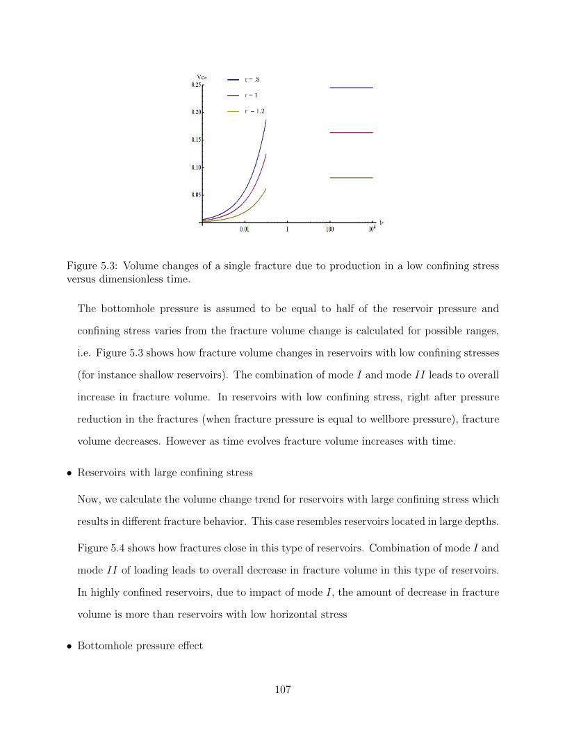
Figure 5.3: Volume changes of a single fracture due to production in a low confining stressversus dimensionless time.

The bottomhole pressure is assumed to be equal to half of the reservoir pressure and

confining stress varies from the fracture volume change is calculated for possible ranges,

i.e. Figure 5.3 shows how fracture volume changes in reservoirs with low confining stresses

(for instance shallow reservoirs). The combination of mode I and mode II leads to overall

increase in fracture volume. In reservoirs with low confining stress, right after pressure

reduction in the fractures (when fracture pressure is equal to wellbore pressure), fracture

volume decreases. However as time evolves fracture volume increases with time.

• Reservoirs with large confining stress

Now, we calculate the volume change trend for reservoirs with large confining stress which

results in different fracture behavior. This case resembles reservoirs located in large depths.

Figure 5.4 shows how fractures close in this type of reservoirs. Combination of mode I and

mode II of loading leads to overall decrease in fracture volume in this type of reservoirs.

In highly confined reservoirs, due to impact of mode I, the amount of decrease in fracture

volume is more than reservoirs with low horizontal stress

• Bottomhole pressure effect

107

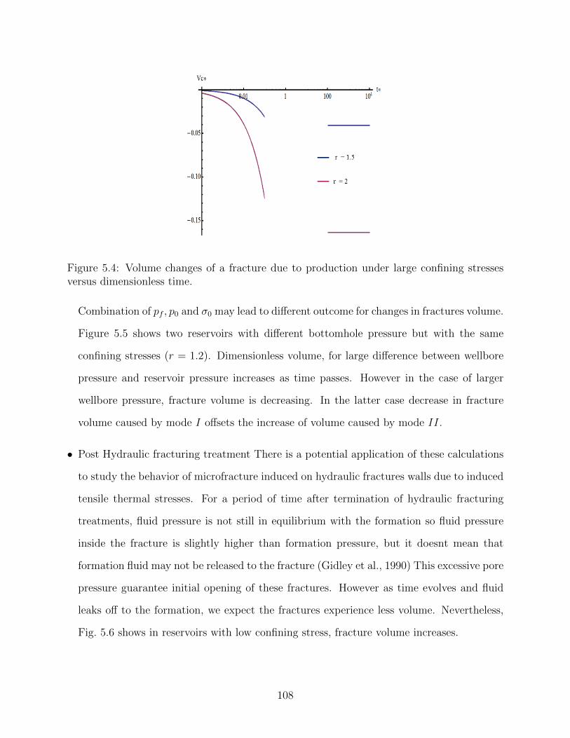
Figure 5.4: Volume changes of a fracture due to production under large confining stressesversus dimensionless time.

Combination of pf , p0 and σ0 may lead to different outcome for changes in fractures volume.

Figure 5.5 shows two reservoirs with different bottomhole pressure but with the same

confining stresses (r = 1.2). Dimensionless volume, for large difference between wellbore

pressure and reservoir pressure increases as time passes. However in the case of larger

wellbore pressure, fracture volume is decreasing. In the latter case decrease in fracture

volume caused by mode I offsets the increase of volume caused by mode II.

• Post Hydraulic fracturing treatment There is a potential application of these calculations

to study the behavior of microfracture induced on hydraulic fractures walls due to induced

tensile thermal stresses. For a period of time after termination of hydraulic fracturing

treatments, fluid pressure is not still in equilibrium with the formation so fluid pressure

inside the fracture is slightly higher than formation pressure, but it doesnt mean that

formation fluid may not be released to the fracture (Gidley et al., 1990) This excessive pore

pressure guarantee initial opening of these fractures. However as time evolves and fluid

leaks off to the formation, we expect the fractures experience less volume. Nevertheless,

Fig. 5.6 shows in reservoirs with low confining stress, fracture volume increases.

108

Figure 5.5: Volume changes of a fracture due to production under large confining stressesversus dimensionless time.

Figure 5.6: Volume changes of a fracture due to production under large confining stressesversus dimensionless time.

109

5.5 Conclusion

We presented poroelastic solution for the drainage of a single microfracture. Moreover we

investigated the effects of formation pressure, rock mechanical properties, insitu stress and

bottomhole pressure on the volume of the fractures. Since, fractures width changes affect

their hydraulic conductivity and subsequently overall permeability of reservoirs, therefore

production could be affected by the change of fractures volume.

It has been shown that the difference between bottomhole pressure and reservoir pressure

results in the augmentation of the fracture volume. This increase may be counterbalanced

by large horizontal stresses in the reservoir. In case of reservoirs with low confining stresses,

fracture volume increases with time. However, in reservoirs with large confining stress, the

fracture volume is decreasing. Additionally, we showed bottomhole pressure changes under

certain condition could change reverse behavior of the poroelastic fractures in the reservoir.

The poroelastic response of the fractures is not the only factor which influences the

reservoir productivity. Other aspects such as the presence of multiphase fluids should also

be considered in further analyses in future. Here, we considered plane strain geometry

for natural fractures. It might be more realistic to consider penny shaped fractures with

axisymmetric geometry for this problem as well. The next step will be the investigation of

the effect of numerous micro-fractures on the major macro-size fracture and its productivity.

5.6 References

Aguilera, R., 2008. Role of natural fractures and slot porosity on tight gas sands, in: Pro-ceedings of SPE Unconventional Reservoirs Conference, Society of Petroleum Engineers.pp. 10–12. doi:10.2118/114174-MS.

Ali, W.A., 2009. Lithofacies, depositional environment, burial history and calculation oforganic richness from the wireline logs: a study of Barnett Shale in the Delaware Basin,Pecos Co., West Texas, and comparison with the Barnett Shale in the Fort Worth Basin.Ph.D. thesis. University of Texas at Austin.

110

Atkinson, C., Craster, R.V., 1991. Plane strain fracture in poroelastic media. Proceedingsof the Royal Society A: Mathematical, Physical and Engineering Sciences 434, 605–633.doi:10.1098/rspa.1991.0116.

Barree, R.D., 1998. Applications of pre-frac injection/falloff tests in fissured reservoirs - fieldexamples, in: Proceedings of SPE Rocky Mountain Regional/Low-Permeability ReservoirsSymposium, Society of Petroleum Engineers. doi:10.2118/39932-MS.

Biot, M.A., 1941. General theory of three-dimensional consolidation. Journal of AppliedPhysics 12, 155. doi:10.1063/1.1712886.

Bonnet, E., Bour, O., Odling, N.E., Davy, P., Main, I., Cowie, P., Berkowitz, B., 2001.Scaling of fracture systems in geological media. Reviews of Geophysics 39, 347. doi:10.1029/1999RG000074.

Britt, L.K., Hager, C.J., Thompson, J.W., 1994. Hydraulic fracturing in a naturally fracturedreservoir, in: Proceedings of International Petroleum Conference and Exhibition of Mexico,Society of Petroleum Engineers. doi:10.2118/28717-MS.

Carslaw, H.S., Jaeger, J.C., 1959. Conduction of heat in solids. Second edi ed., OxfordUniversity Press, London.

Cleary, M.P., 1977. Fundamental solutions for a fluid-saturated porous solid. InternationalJournal of Solids and Structures 13, 785–806. doi:10.1016/0020-7683(77)90065-8.

Craster, R.V., Atkinson, C., 1994. Crack problems in a poroelastic medium: an asymptoticapproach. Philosophical Transactions of the Royal Society A: Mathematical, Physical andEngineering Sciences 346, 387–428. doi:10.1098/rsta.1994.0026.

Dahi Taleghani, A., 2011. Modeling simultaneous growth of multi-branch hydraulic fractures,in: 45th US Rock Mechanics/Geomechanics Symposium, San Francisco, CA.

Dahi Taleghani, A., Olson, J.E., 2011. Numerical modeling of multistranded-hydraulic-fracture propagation: Accounting for the interaction between induced and natural frac-tures. SPE Journal , 575–581.

David, C., Ravalec-Dupin, M.L., 2007. Rock physics and geomechanics in the study ofreservoirs and repositories. Geological Society, London, Special Publications 284, 1–14.

111

Detournay, E., Cheng, A.H.D., 1991. Plane strain analysis of a stationary hydraulic fracturein a poroelastic medium. International Journal of Solids and Structures 27, 1645–1662.doi:10.1016/0020-7683(91)90067-P.

Engelder, T., Lacazette, A., 1990. Natural hydraulic fracturing, in: Barton, N., Stephansson,O. (Eds.), International Symposium on Rock Joints.

Gale, J.F.W., 2002. Specifying lengths of horizontal wells in fractured reservoirs. SPEReservoir Evaluation & Engineering 5. doi:10.2118/78600-PA.

Gale, J.F.W., Lander, R.H., Reed, R.M., Laubach, S.E., 2010. Modeling fracture porosityevolution in dolostone. Journal of Structural Geology 32, 1201–1211. doi:10.1016/j.jsg.2009.04.018.

Gale, J.F.W., Reed, R.M., Holder, J., 2007. Natural fractures in the Barnett Shale and theirimportance for hydraulic fracture treatments. AAPG Bulletin 91, 603–622. doi:10.1306/11010606061.

Gangi, A.F., Carlson, R.L., 1996. An asperity-deformation model for effective pressure.Tectonophysics 256, 241–251. doi:10.1016/0040-1951(95)00167-0.

Ghassemi, A., Zhang, Q., 2006. Porothermoelastic analysis of the response of a stationarycrack using the displacement discontinuity method. Journal of Engineering Mechanics 132,26–33. doi:10.1061/(ASCE)0733-9399(2006)132:1(26).

Gidley, J.L., Holditch, S.A., Nierode, D.E., Jr., R.W.V. (Eds.), 1990. Recent advances inhydraulic fracturing. Society of Petroleum Engineers.

Gillespie, P.A., Howard, C.B., Walsh, J.J., Watterson, J., 1993. Measurement and charac-terisation of spatial distributions of fractures. Tectonophysics 226, 113–141. doi:10.1016/0040-1951(93)90114-Y.

Gilman, J., Kazemi, H., 1988. Improved calculations for viscous and gravity displacementin matrix blocks in dual-porosity simulators (includes associated papers 17851, 17921,18017, 18018, 18939, 19038, 19361 and 20174 ). Journal of Petroleum Technology 40.doi:10.2118/16010-PA.

112

Heffer, K.J., Last, N.C., Koutsabeloulis, N.C., Gutierrez, M., Makurat, A., 1995. Site-response models from high-resolution seismic reflection and refraction data recorded inSanta Cruz, California. International Journal of Rock Mechanics and Mining Sciences &Geomechanics Abstracts 32.

Kazemi, H., 1982. Low-permeability gas sands. Journal of Petroleum Technology 34, 2229–2232. doi:10.2118/11330-PA.

Koutsabeloulis, N.C., Heffer, K.J., Wong, S., 1994. Numerical geomechanics in reservoirengineering. Computer Methods and Advances in Geomechanics 92.

Laubach, S.E., 2003. Practical approaches to identifying sealed and open fractures. AAPGbulletin 4, 561–579.

Laubach, S.E., Olson, J.E., Gale, J.F.W., 2004. Are open fractures necessarily alignedwith maximum horizontal stress? Earth and Planetary Science Letters 222, 191–195.doi:10.1016/j.epsl.2004.02.019.

Marrett, R., Ortega, O.J., Kelsey, C.M., 1999. Extent of power-law scaling for naturalfractures in rock. Geology 27, 799. doi:10.1130/0091-7613(1999)027<0799:EOPLSF>2.3.CO;2.

Olson, J.E., Laubach, S.E., Lander, R.H., 2009. Natural fracture characterization in tightgas sandstones: Integrating mechanics and diagenesis. AAPG Bulletin 93, 1535–1549.doi:10.1306/08110909100.

Philip, Z., Jennings, J., Olson, J.E., Laubach, S.E., Holder, J., 2005. Modeling coupledfracture-matrix fluid flow in geomechanically simulated fracture networks. SPE ReservoirEvaluation & Engineering 8. doi:10.2118/77340-PA.

Sneddon, I.N., 1946. The distribution of stress in the neighbourhood of a crack in anelastic solid. Proceedings of the Royal Society A: Mathematical, Physical and EngineeringSciences 187, 229–260. doi:10.1098/rspa.1946.0077.

Valko, P., Economides, M.J., 1995. Hydraulic fracture mechanics. UK: Wiley.

113

Vandamme, L., Detournay, E., Cheng, A.H.D., 1989. A two-dimensional poroelastic dis-placement discontinuity method for hydraulic fracture simulation. International Journalfor Numerical and Analytical Methods in Geomechanics 13, 215–224. doi:10.1002/nag.1610130209.

114

Chapter 6Pressurized Poroelastic Inclusions: Short-term and Long-term Asymptotic Solu-tions

This paper provides a semi-analytical asymptotic short-term and long-term solutions for the

volume change and the corresponding leak-off volume for a fluid saturated three-dimensional

poroelastic inclusion considering fluid exchange with the surrounding poroelastic medium.

Considering possibly different material properties and different fluid pressure of hydrocarbon

bearing formations or proppant filled fractures in comparison to those of the surrounding

geological structures, fractures or the whole reservoirs can be considered as inclusions. The

approach used for solving this problem is inspired by the theory of inclusions and modal

decomposition technique previously developed and used to solve several poroelasticity prob-

lems. Previous studies on the topic have not incorporated the hydraulic communication

between the inclusion and the surrounding medium; therefore, fluid pressure changes in the

surrounding rock due fluid pressure changes in the inclusion was ignored. An example of this

problem would be a pressurized stationary fracture, which depending on pressure might have

fluid exchange with the surroundings. Some numerical examples considering inclusions with

different aspect ratios and material properties are provided to better describe the significance

of fluid exchange.

115

6.1 Introduction

This paper provides a semi-analytical asymptotic short-term and long-term solutions for the

volume change and the corresponding leak-off volume for a fluid saturated three-dimensional

poroelastic inclusion considering fluid exchange with the surrounding poroelastic medium

(see Fig. 6.1).

Inclusions are defined as finite sub-volumes of the medium, which may possess a different

strain status from that of the surrounding environment. If the inclusion has different material

properties, it is considered to be an inhomogeneous inclusion. Considering possibly different

material properties and different fluid pressure of hydrocarbon bearing formations or prop-

pant filled fractures in comparison to those of the surrounding geological structures, fractures

or the whole reservoirs can be considered as inclusions. For example Rudnicki (2002a,b);

Chen (2011); Soltanzadeh and Hawkes (2012); Bedayat and Dahi Taleghani (2014) modeled

stress alterations in the poroelastic inclusions due to pore fluid pressure changes using the

theory of the inclusions. All these studies assumed that there is no hydraulic communication

between the inclusion and the surrounding medium. Therefore, the fluid pressure in the

surrounding rock will not change due to fluid pressure changes in the inclusion and there is

no fluid exchange with the matrix. However, these assumptions are reasonable for model-

ing situations like rock compaction-drive and gas expansion-drive hydrocarbon reservoirs, as

well as for geological carbon sequestration. The lack of hydraulic communication could be

the result of a cap rock or an impermeable fault. For example, high permeability sandstone

formations could be contained by extremely less permeable shale layers.

Here, we solved for the volume change of an ellipsoidal poroelastic inclusion and its cor-

responding leak-off volume, assuming hydraulic communication between the inclusion and

the matrix. An example of this problem would be a pressurized stationary fracture, which

depending on pressure might have fluid exchange with the surroundings. It is notable that,

pressurized elliptical fractures can be considered as a special case of ellipsoidal inclusions

116

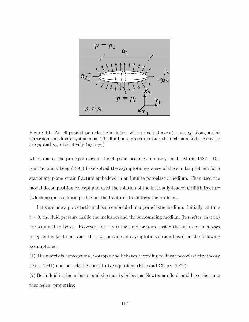
𝑎1

𝑎2 𝑎3

𝑝 = 𝑝0

𝑝 = 𝑝𝐼𝑝𝐼 > 𝑝0

Figure 6.1: An ellipsoidal poroelastic inclusion with principal axes (a1, a2, a3) along majorCartesian coordinate system axis. The fluid pore pressure inside the inclusion and the matrixare pI and p0, respectively (pI > p0).

where one of the principal axes of the ellipsoid becomes infinitely small (Mura, 1987). De-

tournay and Cheng (1991) have solved the asymptotic response of the similar problem for a

stationary plane strain fracture embedded in an infinite poroelastic medium. They used the

modal decomposition concept and used the solution of the internally-loaded Griffith fracture

(which assumes elliptic profile for the fracture) to address the problem.

Let’s assume a poroelastic inclusion embedded in a poroelastic medium. Initially, at time

t = 0, the fluid pressure inside the inclusion and the surrounding medium (hereafter, matrix)

are assumed to be p0. However, for t > 0 the fluid pressure inside the inclusion increases

to pI and is kept constant. Here we provide an asymptotic solution based on the following

assumptions :

(1) The matrix is homogenous, isotropic and behaves according to linear poroelasticity theory

(Biot, 1941) and poroelastic constitutive equations (Rice and Cleary, 1976);

(2) Both fluid in the inclusion and the matrix behave as Newtonian fluids and have the same

rheological properties;

117

(3) The matrix is subjected to uniform far-field stresses σx = σy = σz = σ0;

The outline of this paper is as follows: Section 6.2 describes the approach used for

solving this problem. In Section 6.2.1 we review the governing equations used to solve the

asymptotic volume change of the poroelastic inhomogeneity, and in Section 6.2.3 we describe

the Eshelby solution for poroelastic inclusions. Then in Section 6.3, we describe our approach

to solve the volume change of the inclusion for short term and long term responses. Finally,

Some numerical examples considering inclusions with different aspect ratios and material

properties are provided to better describe the significance of fluid exchange toward the end

of the paper.

6.2 Solution Methods

6.2.1 General approach

The approach used for solving this problem is inspired by modal decomposition and su-

perposition method previously developed and used to solve several poroelasticity problems

such as sudden pressurization of a borehole (Detournay and Cheng, 1988) and plain strain

stationary fracture (Detournay and Cheng, 1991). Considering that the normal traction and

pore pressure along the inclusion surface is equal to the fluid pressure inside the inclusion

(σn = −pI , p = pI), the response of the inclusion can be decomposed into two fundamental

problems: (1) a step change in stress while there is no pore pressure change inside the inclu-

sion (σn = −1(0,∞], p = 0); (2) a step change in pore pressure while there is no stress change

inside the inclusion (σn = 0, p = 1(0,∞]). Therefore, the inclusion response in the general

condition can be considered as a linear combination of each of these modes. Here, we assume

that there is no initial pore pressure difference between the inclusion and the surrounding

matrix, and pore pressure inside the inclusion increases immediately to pI and it will not

change by time. However, in cases when pressure varies with time, Duhamel’s theorem can

be applied (see Section 6.7). Thus, the boundary conditions for the two fundamental loading

118

modes are

Mode (1) =

σn(x, t) = −1

p(x, t) = 0,(6.1)

and

Mode (1) =

σn(x, t) = 0

p(x, t) = 1,(6.2)

Let ∆V(1)I and ∆V

(2)I be the volume change of the inclusion for mode (1) and mode (2),

respectively. Therefore, in the presence of compressive in-situ stresses (σ0), and the matrix

initial pore pressure (p0), the solution for change in the inclusion volume may be given as

∆VI(pI) = pI∆V(1)I + (pI − p0)∆V

(2)I . (6.3)

The asymptotic values of ∆V(1)I and ∆V

(2)I are calculated in Section 6.3, which can be

substituted in to find the final volume of the inclusion.

6.2.2 Governing equations of poroelastic medium

The governing equations for solving this problem can be categorized into four different

groups: force equilibrium equations, fluid flow (Darcy’s law), mass balance and Biots con-

stitutive equations (Biot, 1941) :

(1) Force equilibrium equations

σij,j = 0, (6.4)

where σij is the total stress.

119

(2) Darcy’s law, is used to describe the fluid transport in the rock. By neglecting the gravity

effect, Darcy’s law can be written as

qi = −kijµ

∂p

∂xj= −κp,i, (6.5)

where p is the fluid pressure; q is the specific discharge vector; xi indicates the flow direction;

kij is the permeability tensor; µ is the dynamic viscosity of the fluid; and κ is the mobility

ratio.

(3) Continuity equation or mass balance for the fluid phase can be written as

∂ζ

∂t+ qi,i = 0, (6.6)

where t is time; and ζ is incremental fluid content and is defined as

ζ =δmf

ρf0, (6.7)

where δmf is the mass change of pore fluid; and ρf0 is the density of the fluid in the reference

state.

(4) Biot’s poroelastic constitutive equations, is used to describe the constitutive equations

for a fluid-filled porous media. Linear and reversible relationship between stresses (σij, p) on

one side and kinematics i.e. strains and fluid content (εij, ζ) on the other side are implied

in Biot theory. The Biot’s constitutive equations for isotropic poroelastic materials can be

written as

εij =1

2G

[σij −

(3K − 2G

9K

)σkkδij +

2G

3Kαpδij

], (6.8)

ζ =α

K

(σkk3

+p

B

), (6.9)

120

where δij is the Kronecker delta (δij = 1 for i = j, and δij = 0 for i 6= j), εij and σij are the

components of strain and stress tensor in the solid matrix, respectively; and p is the pore

fluid pressure. There are four material constants in the poroelastic constitutive equations:

the Biot coefficient α; drained bulk modulus K; shear modulus G; and B the Skempton’s

coefficient

B =3(νu − ν)

α(1− 2ν)(1 + νu), (6.10)

where ν and νu are drained and undrained Poisson’s ratio, respectively.

The combination of all these equations to solve the time-dependent interaction of rock

deformation and fluid flow for the case of no fluid source, is given by the inhomogeneous

diffusion equation for pore pressure

B

3

∂σkk∂t

+∂p

∂t= c∇2p, (6.11)

where c is the diffusivity coefficient

c =2(1− ν)(1 + νu)

2

9(1− νu)(νu − ν)κGB2. (6.12)

6.2.3 Poroelastic inclusions

Consider an ellipsoidal inclusion in an infinite elastic solid, which undergoes a uniform eigen-

strain εTij, the applied strains in the absence of the surrounding material. Eshelby (1957,

1959) showed that the actual strain and stress inside the inclusion are uniform and given by

εij = SijklεTkl, (6.13)

σij = C0ijkl[εkl − εTkl], (6.14)

121

where εij and σij are the components of strain and stress tensors in the matrix, respectively;

C0ijkl is the elastic moduli of the matrix; and Eshelby tensor Sijkl, is a fourth rank tensor which

is a function of geometry and Poisson’s ratio of the ellipsoidal inclusion (see Mura (1987)

for more details). Rudnicki (2002a) combined the Eshelby formulation and constitutive

equations of poroelastic medium Eq. (6.8) and (6.14) to solve the pressurized poroelastic

inclusion problem. Considering a poroelastic pressurized inclusion, the eigenstrain εT (which

is the stress-free transformation strain) can be obtained by setting σij = 0 in Eq. (6.8)

εTmn = C−1mnijαijp = Lmnijαijp, (6.15)

where Lmnij is the tensor of elastic compliances, inverse of Cmnij. Therefore the corresponding

strain field can be calculated from Eq. (6.13). Obtaining strain field inside the inclusion, the

inclusion volume change may be calculated using volumetric strain times the initial volume

as

∆VI = εTkkV0. (6.16)

The volume change calculated in Eq. (6.16) does not consider fluid leak-off from the inclu-

sion. The effect of fluid diffusion from the inclusion to the matrix is considered in calculating

the asymptotic inclusion volume analysis.

6.3 Asymptotic Analysis

6.3.1 Mode (1) loading

Short term response for the inclusion volume. Let’s assume an ellipsoidal inhomo-

geneity is embedded in an infinite medium and it is pressurized with unit uniform pressure.

According to Eq. (6.16), the volume change of the inhomogeneity ∆VI right after the change

122

of the fluid pressure on the inhomogeneity surface (at t = 0+) can be calculated from

∆V(1)I (0+) = εkkV

0I , assuming undrained material conditions. (6.17)

Subsequently, at t = 0+ due to the application of the unit normal stress σn = −1 on the

inclusion wall, an area with excessive pore pressure generates near the inhomogeneity surface.

The magnitude of the pore pressure in this area can be calculated considering the undrained

elastic response of the inhomogeneity ( ζ = 0 in Eq. (6.9)). Hence the excessive pore pressure

value in the inhomogeneity vicinity is

limt→0+

p = −B3σkk = B, (6.18)

which causes fluid flow from the inhomogeneity surface to the matrix and it can be modeled

similar to mode (2) loading behavior (see Section 6.3.1) and Eq. (6.21)). Thus the final

volume change of the inhomogeneity is

∆V(1)I (t) = ∆V

(1)I (0+) + (−B)∆V

(2)I (t). (6.19)

Long term response for the inclusion volume. Consider the condition for long enough

time , i.e. time evolves to infinity. The pore pressure generated by the mode (1) loading

near the inhomogeneity surface (see Eq. (6.18)) should dissipate, therefore the second term

in Eq. (6.19) vanishes. Hence, the long-term volume change can be calculated similar to Eq.

(6.17) but using drained material properties

∆V(1)I (∞) = εkkV0. (6.20)

Short term response for the leak-off volume. As mentioned before, the pore pres-

sure field generated in Eq. (6.18) should dissipate, due to pressure gradient in the matrix.

123

According to Section 6.6, the fluid flux Q√A for a unit pressure difference between an ellip-

soidal surface with surface area equal to A (here, the inhomogeneity) and the matrix can be

approximate as

Q√A = κ√A

1√π√

ctA

((S∗√

A

√π

√ct

A

)n

+ 1

) 1n

, (6.21)

where t is the actual time; S∗√A

is the dimensionless conduction shape factor; and n is

the blending coefficient (see Table 6.2). Consequently by integrating the flux over time

on the inclusion surface, and multiplying the pore pressure drop calculated in Eq. (6.18)

(∆p = −B), the fluid leak-off volume for short time scale ( ctA 1) will be

V(1)l (t) = −B

∫ t

0

Q√Adt

=2BκA

√t√

c√π

2F1

(− 1

n,

1

n; 1 +

1

n;−(S∗√

A

√π)n(ct

A

)n2

), (6.22)

where 2F1(a, b; c; z) is the Gauss’s hypergeometric function. The negative sign in Eq. (6.22)

indicates fluid flow toward the inclusion.

Long term response for the leak-off volume. Considering that no fluid exchange

between the matrix and its boundary after prolonged time, the long term leak-off volume

can be calculated as the integration of increment of fluid content ζ|t=∞ over the isopressure

surface and has the form

V(1)l (∞) =

∫t

Q√A =

∫V

ζ|t=∞dV. (6.23)

On the other hand, as time evolves to infinity the excess pore pressure in the matrix will

dissipate (p = 0). Therefore from Eq. (6.8) and (6.9) and solving for ζ we get

limt→+∞

ζ = α limt→+∞

εkk. (6.24)

124

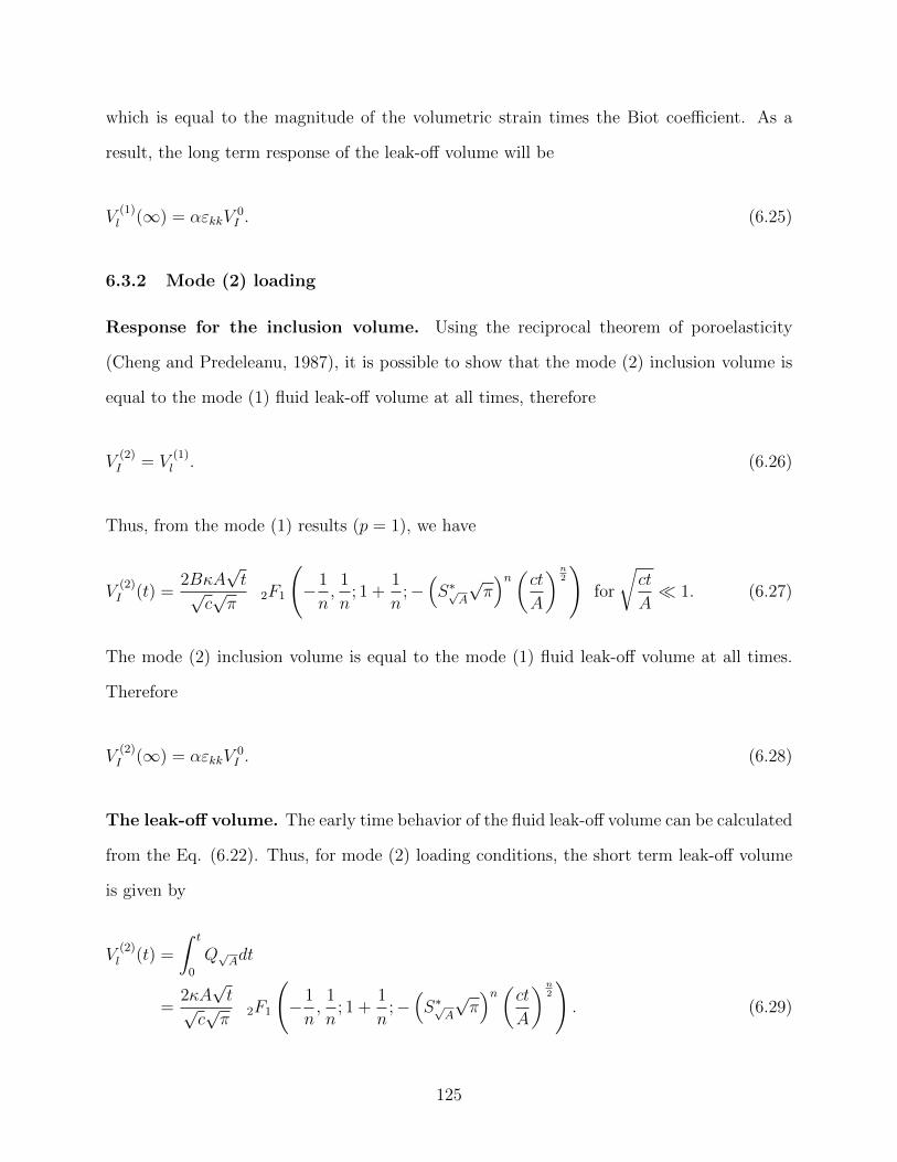
which is equal to the magnitude of the volumetric strain times the Biot coefficient. As a

result, the long term response of the leak-off volume will be

V(1)l (∞) = αεkkV

0I . (6.25)

6.3.2 Mode (2) loading

Response for the inclusion volume. Using the reciprocal theorem of poroelasticity

(Cheng and Predeleanu, 1987), it is possible to show that the mode (2) inclusion volume is

equal to the mode (1) fluid leak-off volume at all times, therefore

V(2)I = V

(1)l . (6.26)

Thus, from the mode (1) results (p = 1), we have

V(2)I (t) =

2BκA√t√

c√π

2F1

(− 1

n,

1

n; 1 +

1

n;−(S∗√

A

√π)n(ct

A

)n2

)for

√ct

A 1. (6.27)

The mode (2) inclusion volume is equal to the mode (1) fluid leak-off volume at all times.

Therefore

V(2)I (∞) = αεkkV

0I . (6.28)

The leak-off volume. The early time behavior of the fluid leak-off volume can be calculated

from the Eq. (6.22). Thus, for mode (2) loading conditions, the short term leak-off volume

is given by

V(2)l (t) =

∫ t

0

Q√Adt

=2κA√t√

c√π

2F1

(− 1

n,

1

n; 1 +

1

n;−(S∗√

A

√π)n(ct

A

)n2

). (6.29)

125

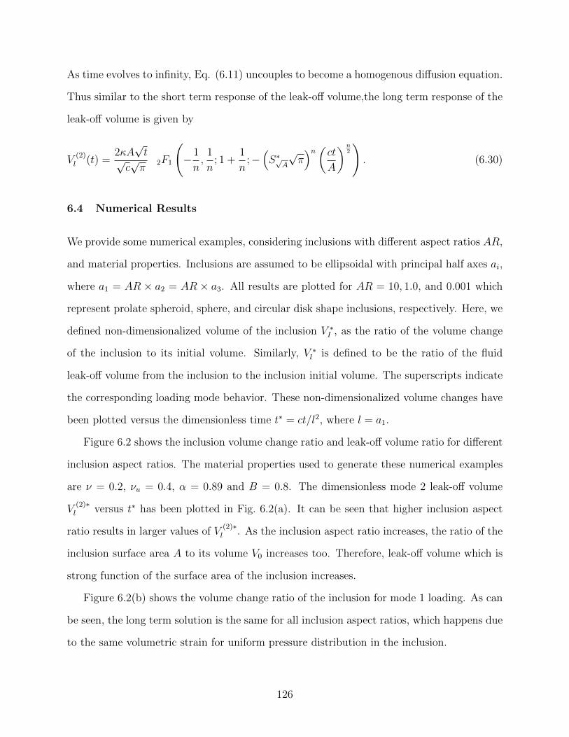
As time evolves to infinity, Eq. (6.11) uncouples to become a homogenous diffusion equation.

Thus similar to the short term response of the leak-off volume,the long term response of the

leak-off volume is given by

V(2)l (t) =

2κA√t√

c√π

2F1

(− 1

n,

1

n; 1 +

1

n;−(S∗√

A

√π)n(ct

A

)n2

). (6.30)

6.4 Numerical Results

We provide some numerical examples, considering inclusions with different aspect ratios AR,

and material properties. Inclusions are assumed to be ellipsoidal with principal half axes ai,

where a1 = AR × a2 = AR × a3. All results are plotted for AR = 10, 1.0, and 0.001 which

represent prolate spheroid, sphere, and circular disk shape inclusions, respectively. Here, we

defined non-dimensionalized volume of the inclusion V ∗I , as the ratio of the volume change

of the inclusion to its initial volume. Similarly, V ∗l is defined to be the ratio of the fluid

leak-off volume from the inclusion to the inclusion initial volume. The superscripts indicate

the corresponding loading mode behavior. These non-dimensionalized volume changes have

been plotted versus the dimensionless time t∗ = ct/l2, where l = a1.

Figure 6.2 shows the inclusion volume change ratio and leak-off volume ratio for different

inclusion aspect ratios. The material properties used to generate these numerical examples

are ν = 0.2, νu = 0.4, α = 0.89 and B = 0.8. The dimensionless mode 2 leak-off volume

V(2)∗l versus t∗ has been plotted in Fig. 6.2(a). It can be seen that higher inclusion aspect

ratio results in larger values of V(2)∗l . As the inclusion aspect ratio increases, the ratio of the

inclusion surface area A to its volume V0 increases too. Therefore, leak-off volume which is

strong function of the surface area of the inclusion increases.

Figure 6.2(b) shows the volume change ratio of the inclusion for mode 1 loading. As can

be seen, the long term solution is the same for all inclusion aspect ratios, which happens due

to the same volumetric strain for uniform pressure distribution in the inclusion.

126

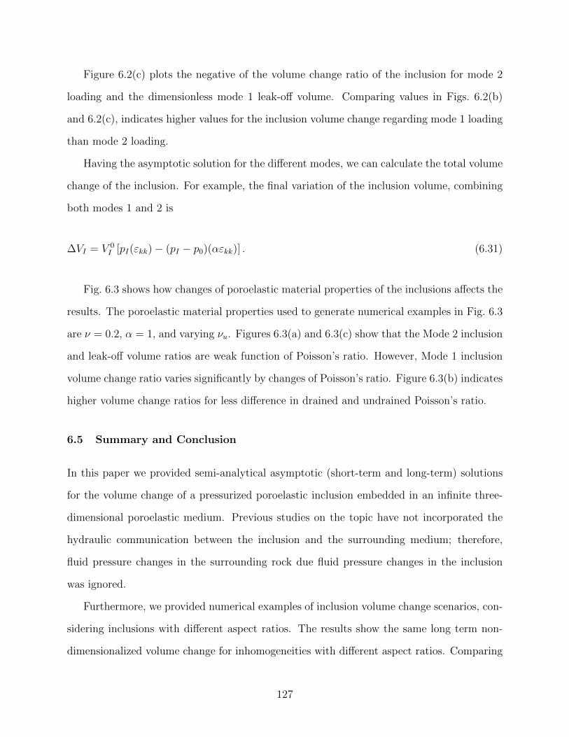
Figure 6.2(c) plots the negative of the volume change ratio of the inclusion for mode 2

loading and the dimensionless mode 1 leak-off volume. Comparing values in Figs. 6.2(b)

and 6.2(c), indicates higher values for the inclusion volume change regarding mode 1 loading

than mode 2 loading.

Having the asymptotic solution for the different modes, we can calculate the total volume

change of the inclusion. For example, the final variation of the inclusion volume, combining

both modes 1 and 2 is

∆VI = V 0I [pI(εkk)− (pI − p0)(αεkk)] . (6.31)

Fig. 6.3 shows how changes of poroelastic material properties of the inclusions affects the

results. The poroelastic material properties used to generate numerical examples in Fig. 6.3

are ν = 0.2, α = 1, and varying νu. Figures 6.3(a) and 6.3(c) show that the Mode 2 inclusion

and leak-off volume ratios are weak function of Poisson’s ratio. However, Mode 1 inclusion

volume change ratio varies significantly by changes of Poisson’s ratio. Figure 6.3(b) indicates

higher volume change ratios for less difference in drained and undrained Poisson’s ratio.

6.5 Summary and Conclusion

In this paper we provided semi-analytical asymptotic (short-term and long-term) solutions

for the volume change of a pressurized poroelastic inclusion embedded in an infinite three-

dimensional poroelastic medium. Previous studies on the topic have not incorporated the

hydraulic communication between the inclusion and the surrounding medium; therefore,

fluid pressure changes in the surrounding rock due fluid pressure changes in the inclusion

was ignored.

Furthermore, we provided numerical examples of inclusion volume change scenarios, con-

sidering inclusions with different aspect ratios. The results show the same long term non-

dimensionalized volume change for inhomogeneities with different aspect ratios. Comparing

127

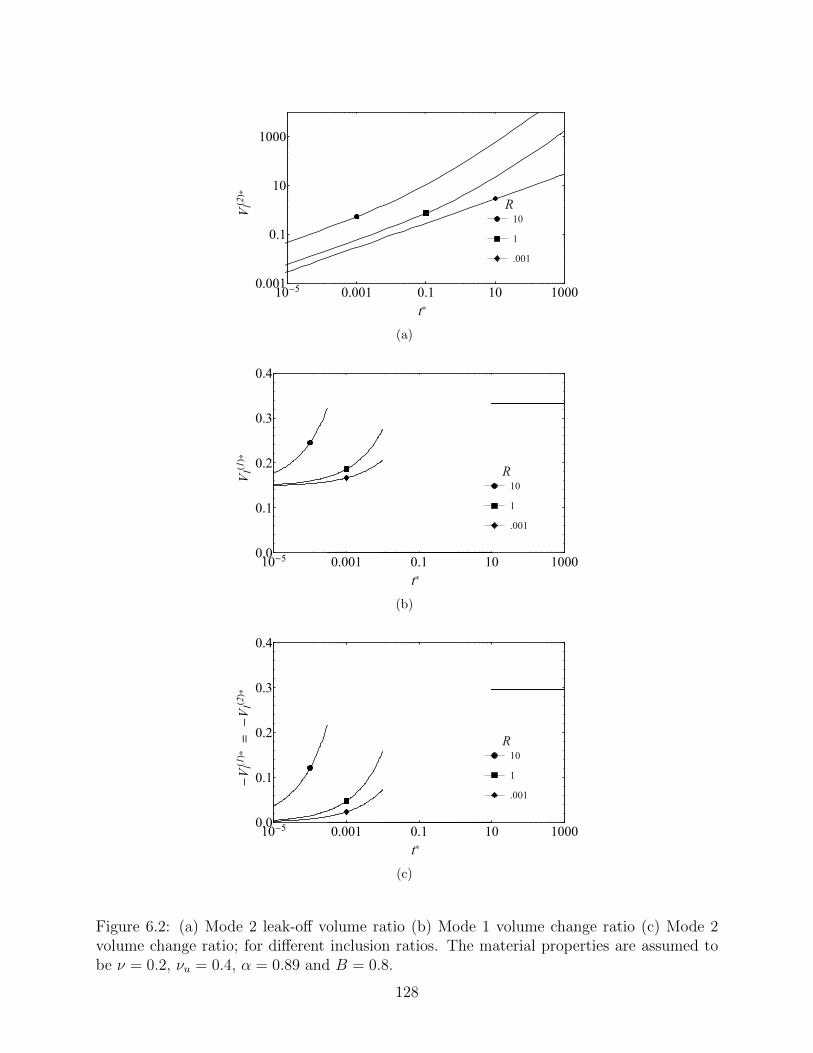
R

10

1

.001

10-5

0.001 0.1 10 10000.001

0.1

10

1000

t*

VlH

2L*

(a)

R

10

1

.001

10-5

0.001 0.1 10 10000.0

0.1

0.2

0.3

0.4

t*

VIH1

L*

(b)

R

10

1

.001

10-5

0.001 0.1 10 10000.0

0.1

0.2

0.3

0.4

t*

-V

lH1

L*

=-

VIH2

L*

(c)

Figure 6.2: (a) Mode 2 leak-off volume ratio (b) Mode 1 volume change ratio (c) Mode 2volume change ratio; for different inclusion ratios. The material properties are assumed tobe ν = 0.2, νu = 0.4, α = 0.89 and B = 0.8.

128

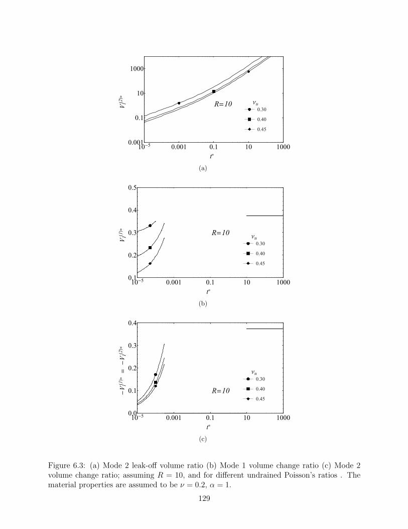
R=10 nu

0.30

0.40

0.45

10-5

0.001 0.1 10 10000.001

0.1

10

1000

t*

VlH

2L*

(a)

R=10nu

0.30

0.40

0.45

10-5

0.001 0.1 10 10000.1

0.2

0.3

0.4

0.5

t*

VIH1

L*

(b)

R=10

nu

0.30

0.40

0.45

10-5

0.001 0.1 10 10000.0

0.1

0.2

0.3

0.4

t*

-V

lH1

L*

=-

VIH2

L*

(c)

Figure 6.3: (a) Mode 2 leak-off volume ratio (b) Mode 1 volume change ratio (c) Mode 2volume change ratio; assuming R = 10, and for different undrained Poisson’s ratios . Thematerial properties are assumed to be ν = 0.2, α = 1.

129

non-dimensionalized volume change values of mode 1 and mode 2 loadings, indicates higher

values for mode 1 loading condition.

Results show that the Mode 2 inclusion and leak-off volume ratios are weak function

of Poisson’s ratio. However, Mode 1 inclusion volume change ratio varies significantly by

changes of Poisson’s ratio.

6.6 Diffusion equation solution on an ellipsoidal surface

Considering the complete analogy between the heat conduction and the fluid pressure diffu-

sion equations (for example, the Fourier’s law in heat transport is equivalent to the Darcy’s

law in fluid flow, see Table 6.1), the problem of transient fluid diffusion from an isopres-

sure body into the medium can be solved using the available solutions in the literature for

heat conduction from isothermal bodies into an infinite homogenous medium. The non-

Table 6.1: The analogy between heat conduction and fluid diffusion equationsParameter Heat Conduction Fluid Diffusion

Material property Thermal conductivity (k) Mobility (κ)Material property Thermal diffusivity (α) Fluid diffusivity (c)Potential Function Temperature PressureFlux Heat transfer rate Flow rate

dimensional heat diffusion equation in the media can be written as (Yovanovich et al., 1995)

∇2φ(r, τ) =∂φ(r, τ)

∂τ, (6.32)

where

φ(r, τ) =T (r, τ)− T∞T0 − T∞

,

φ(r, τ = 0) = 0,

φ(r = r0, τ > 0) = 1,

130

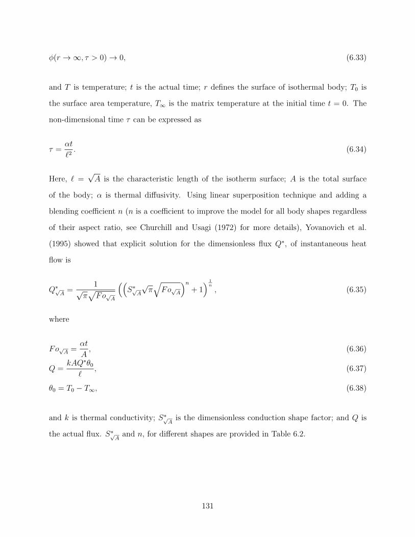
φ(r →∞, τ > 0)→ 0, (6.33)

and T is temperature; t is the actual time; r defines the surface of isothermal body; T0 is

the surface area temperature, T∞ is the matrix temperature at the initial time t = 0. The

non-dimensional time τ can be expressed as

τ =αt

`2. (6.34)

Here, ` =√A is the characteristic length of the isotherm surface; A is the total surface

of the body; α is thermal diffusivity. Using linear superposition technique and adding a

blending coefficient n (n is a coefficient to improve the model for all body shapes regardless

of their aspect ratio, see Churchill and Usagi (1972) for more details), Yovanovich et al.

(1995) showed that explicit solution for the dimensionless flux Q∗, of instantaneous heat

flow is

Q∗√A

=1

√π√Fo√A

((S∗√

A

√π√Fo√A

)n+ 1) 1

n

, (6.35)

where

Fo√A =αt

A, (6.36)

Q =kAQ∗θ0

`, (6.37)

θ0 = T0 − T∞, (6.38)

and k is thermal conductivity; S∗√A

is the dimensionless conduction shape factor; and Q is

the actual flux. S∗√A

and n, for different shapes are provided in Table 6.2.

131

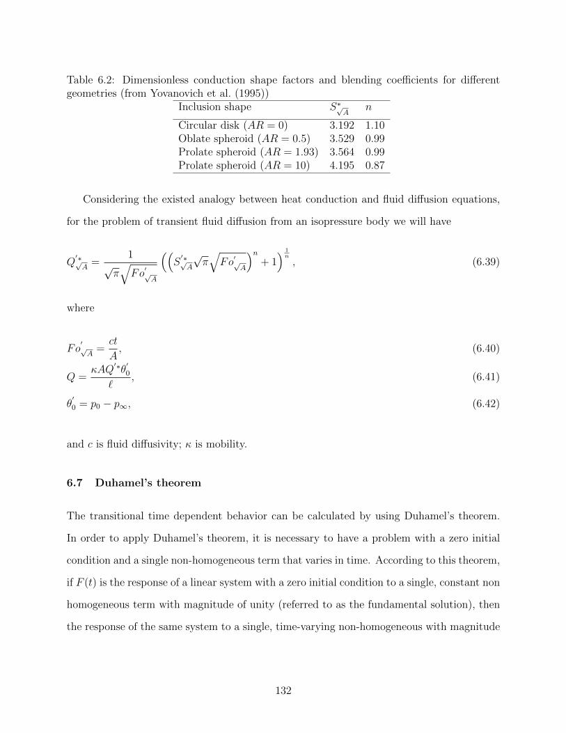
Table 6.2: Dimensionless conduction shape factors and blending coefficients for differentgeometries (from Yovanovich et al. (1995))

Inclusion shape S∗√A

n

Circular disk (AR = 0) 3.192 1.10Oblate spheroid (AR = 0.5) 3.529 0.99Prolate spheroid (AR = 1.93) 3.564 0.99Prolate spheroid (AR = 10) 4.195 0.87

Considering the existed analogy between heat conduction and fluid diffusion equations,

for the problem of transient fluid diffusion from an isopressure body we will have

Q′∗√A

=1

√π√Fo

′√A

((S′∗√A

√π√Fo

′√A

)n+ 1) 1

n

, (6.39)

where

Fo′√A

=ct

A, (6.40)

Q =κAQ

′∗θ′0

`, (6.41)

θ′

0 = p0 − p∞, (6.42)

and c is fluid diffusivity; κ is mobility.

6.7 Duhamel’s theorem

The transitional time dependent behavior can be calculated by using Duhamel’s theorem.

In order to apply Duhamel’s theorem, it is necessary to have a problem with a zero initial

condition and a single non-homogeneous term that varies in time. According to this theorem,

if F (t) is the response of a linear system with a zero initial condition to a single, constant non

homogeneous term with magnitude of unity (referred to as the fundamental solution), then

the response of the same system to a single, time-varying non-homogeneous with magnitude

132

p(t) can be obtained from the fundamental solution according to :

F (t) =

∫ t

τ=0

Tf (t− τ)dp(τ)

dtdτ + p(0)Tf (t). (6.43)

where p(0) is the value of p at t = 0 and p(t) must be continuous in time (Nellis and Klein,

2008).

6.8 References

Bedayat, H., Dahi Taleghani, A., 2014. Interacting double poroelastic inclusions. Mechanicsof Materials 69, 204–212. doi:10.1016/j.mechmat.2013.10.006.

Biot, M.A., 1941. General theory of three-dimensional consolidation. Journal of AppliedPhysics 12, 155. doi:10.1063/1.1712886.

Chen, Z.R., 2011. Poroelastic model for induced stresses and deformations in hydrocar-bon and geothermal reservoirs. Journal of Petroleum Science and Engineering 80, 41–52.doi:10.1016/j.petrol.2011.10.004.

Cheng, A.H.D., Predeleanu, M., 1987. Transient boundary element formulation forlinear poroelasticity. Applied Mathematical Modelling 11, 285–290. doi:10.1016/0307-904X(87)90144-2.

Churchill, S.W., Usagi, R., 1972. A general expression for the correlation of rates of transferand other phenomena. AIChE Journal 18, 1121–1128. doi:10.1002/aic.690180606.

Detournay, E., Cheng, A.H.D., 1988. Poroelastic response of a borehole in a non-hydrostaticstress field. International Journal of Rock Mechanics and Mining Sciences & GeomechanicsAbstracts 25, 171–182. doi:10.1016/0148-9062(88)92299-1.

Detournay, E., Cheng, A.H.D., 1991. Plane strain analysis of a stationary hydraulic fracturein a poroelastic medium. International Journal of Solids and Structures 27, 1645–1662.doi:10.1016/0020-7683(91)90067-P.

133

Eshelby, J.D., 1957. The determination of the elastic field of an ellipsoidal inclusion, andrelated problems. Proceedings of the Royal Society A: Mathematical, Physical and Engi-neering Sciences 241, 376–396. doi:10.1098/rspa.1957.0133.

Eshelby, J.D., 1959. The elastic field outside an ellipsoidal inclusion, in: Proceedings of theRoyal Society of London. Series A, Mathematical and Physical, pp. 561–569.

Mura, T., 1987. Micromechanics of defects in solids. Martinus Nijhoff Publishers.

Nellis, G., Klein, S., 2008. Heat transfer. Cambridge University Press.

Rice, J.R., Cleary, M.P., 1976. Some basic stress diffusion solutions for fluid-saturatedelastic porous media with compressible constituents. Reviews of Geophysics 14, 227.doi:10.1029/RG014i002p00227.

Rudnicki, J.W., 2002a. Alteration of regional stress by reservoirs and other inhomo- geneities:Stabilizing or destabilizing?, in: Vouille, G., Berest, P. (Eds.), Proc. 9th Int. Congr. RockMechanics,Vol. 3, Paris, Aug. 25-29, 1999, Paris, France. pp. 1629– 1637.

Rudnicki, J.W., 2002b. Eshelby transformations, pore pressure and fluid mass changes, andsubsidence, in: Poromechanics II, Proc. 2nd Biot Conference on Poromechanics, Grenoble,France.

Soltanzadeh, H., Hawkes, C.D., 2012. Evaluation of caprock integrity during pore pressurechange using a probabilistic implementation of a closed-form poroelastic model. Interna-tional Journal of Greenhouse Gas Control 7, 30–38. doi:10.1016/j.ijggc.2011.10.006.

Yovanovich, M., Teertstra, P., Culham, J.R., 1995. Modeling transient conduction fromisothermal convex bodies of arbitrary shape. Journal of Thermophysics and Heat Transfer9, 385–390. doi:10.2514/3.678.

134

Chapter 7Summary and Future Works

7.1 Summary

Poroelastic inclusions could have a wide range of applications from rock mechanics problems

to tissue mechanics. For example, many geological phenomena and structures like reservoirs,

aquifers, intrusions, fault zones, caverns, dikes, compaction bands, and other underground

structures can be modeled as inhomogeneous inclusions. Considering different material prop-

erties and different pressure/temperature of hydrocarbon bearing formations in comparison

to those of the surrounding geological structures, hydrocarbon reservoirs and subsurface frac-

tures can be considered as inhomogeneities embedded inside an infinite poroelastic medium.

Moreover, elliptic fractures are special cases of ellipsoidal inhomogeneities when their elastic

moduli are zero, and one of the principal axes of the ellipsoid approaches zero.

This dissertation is comprised of two major interrelated topics. The first focus is to

investigate stress distribution inside and outside of poroelastic inclusions due to alteration

of fluid pressure inside the inclusion (no hydraulic communication between the inclusion and

the surrounding matrix) and its application in reservoir geomechanics (Chapters 2 to 4).

The second objective involves calculating the volume changes of a poroelastic plain strain

fracture/ellipsoidal inclusion due to change of fluid pressure inside the fracture/inclusion,

considering fluid exchange between the inclusion and the matrix (Chapters 5 and 6). The

results obtained from the first topic are directly utilized to investigate the latter subject.

The summary and conclusions of the main results is as follows:

135

An analytical approach for determining stress distribution around two interacting elas-

tic inhomogeneities, was derived for double poroelastic interacting inhomogeneous inclusions.

These inclusions are assumed to be embedded in an infinite elastic medium and under nonuni-

form far-field loading. This method is applicable to three-dimensional problems, and inclu-

sions may be oriented arbitrarily with respect to each other. Using the Equivalent Inclusion

Method (EIM) and polynomial expansion of strain fields in the local coordinate systems, the

solution for two ellipsoidal poroelastic inhomogeneities are derived. To solve this problem

eigenstrains were expanded, and higher order Eshelby’s tensors and their derivatives were

calculated at the center of each inhomogeneity. I found that to get more accurate results, it

is necessary to use more polynomial terms for eigenstrains and higher rank Eshelby’s tensors,

especially when dealing with very close inclusions.

The results show that the distance of centers of the inhomogeneities and their relative

stiffness to the medium affect the associated stress field. Considering same distance for

inhomogeneities, the interaction effect is more significant on stiffer inclusions.

A source code (in Mathematica) to calculate the stress and strain fields inside and outside

of two interacting ellipsoidal inhomogeneities with arbitrary orientation with respect to each

other is developed.

The Equivalent Inclusion Method (EIM) is used to solve for stress and strain distribution

inside and outside of an anisotropic poroelastic inhomogeneity. Finding the equivalent eigen-

strain, graphical results for strain and stress ratio are presented, and further explored the

sensitivity of parameters of different elastic and poroelastic parameters on results assuming

transverse isotropic condition for both poroelastic and elastic parameters of the inhomogene-

ity.

The results show how neglecting the effect of both anisotropic poroelastic and elastic

properties may result in large differences in stress calculations. The stress ratio changes are

much larger in the direction parallel to the axis of symmetry than the directions in the plain

of symmetry.

136

The poroelastic solution for the drainage of a single microfracture considering the effects

of formation pressure, rock mechanical properties, in-situ stress and bottomhole pressure on

the volume of the fractures is derived. Since, fractures width changes affect their hydraulic

conductivity and subsequently overall permeability of reservoirs, therefore production could

be affected by the change of fractures volume.

It has been shown that the difference between bottomhole pressure and reservoir pressure

results in the augmentation of the fracture volume. This increase may be counterbalanced

by large horizontal stresses in the reservoir. In case of reservoirs with low confining stresses,

fracture volume increases with time. However, in reservoirs with large confining stress, the

fracture volume is decreasing. Additionally, it has been shown how the bottomhole pressure

changes under certain condition could change reverse behavior of the poroelastic fractures

in the reservoir.

A semi-analytical asymptotic (short-term and long-term) solutions for the volume change

of a pressurized poroelastic inclusion embedded in an infinite three-dimensional poroelastic

medium are derived. Most previous studies assumed no hydraulic communication between

the inclusion and the surrounding medium; therefore, the fluid pressure in the surrounding

rock will not change due to fluid pressure changes in the inclusion, and there will be no fluid

leak-off from the inclusion.

Numerical examples of inclusion volume change scenarios, considering inclusions with dif-

ferent aspect ratios are provided. The results show the same long term non-dimensionalized

volume change for inhomogeneities with different aspect ratios. The approach used for solv-

ing this problem is inspired by modal decomposition and superposition method previously

developed and used to solve several poroelasticity problems such as sudden pressurization of

a borehole and plain strain stationary fracture. Considering that the normal traction and

pore pressure along the inclusion surface is equal to the fluid pressure inside the inclusion

(σn = −pI , p = pI), the response of the inclusion can be decomposed into two fundamental

problems: (1) a step change in stress while there is no pore pressure change inside the inclu-

137

sion (σn = −1(0,∞], p = 0); (2) a step change in pore pressure while there is no stress change

inside the inclusion (σn = 0, p = 1(0,∞]). Therefore, the inclusion response in the general

condition can be considered as a linear combination of each of these modes.

Comparing non-dimensional volume change for mode 1 and mode 2 loadings, indicates

higher values for the mode 1 loading condition. Results show that the Mode 2 inclusion and

leak-off volume ratios are weak functions of the Poisson’s ratio. However, Mode 1 inclusion

volume change ratio varies significantly with changes of Poisson’s ratio.

7.2 Recommendations for Future Works

The following recommendations are made for possible future research:

• The mechanical modeling of the ellipsoidal poroelastic inhomogeneities can be extended

to non ellipsoidal inhomogeneities using semi analytical methods exist in the damage

mechanics literature.

• Here the surrounding matrix is assumed to be an infinite elastic/poroelastic full space.

The solution of mechanical behavior of the same type of problems in a semi infinite

half space can be used to model some geological structures such as shallow reservoirs

or aquifers.

138

Appendix: Letters of Permission to UsePublished Material

The Permissions from Elsevier publishing company are presented in the following pages:

139

7/9/2014 Rightslink® by Copyright Clearance Center

https://s100.copyright.com/AppDispatchServlet#formTop 1/1

ConferenceProceeding:

Poromechanics V: Proceedingsof the Fifth Biot Conference onPoromechanics

ConferenceProceedingPaper:

The Equivalent InclusionMethod for PoroelasticityProblems

Author: H. Bedayat, A. Dahi Taleghani

Publisher: American Society of CivilEngineers

Date: 06/18/2013

Copyright © 2013, ASCE. All rights reserved.

Logged in as:

Houman Bedayat

Permissions Request

As an ASCE author, you are permitted to reuse you own content for another ASCE or non-ASCEpublication.

Please add the full credit line "With permission from ASCE" to your source citation. Please printthis page for your records.

Type of use: Dissertation/Thesis

Portion: full article

Format: print and electronic

Use of this content will make up more than 25% of the new work: no

Author of this ASCE work or ASCE will publish the new work: yes

Copyright © 2014 Copyright Clearance Center, Inc. All Rights Reserved. Privacy statement. Comments? We would like to hear from you. E-mail us at customercare@copyright.com

140

7/9/2014 Rightslink® by Copyright Clearance Center

https://s100.copyright.com/AppDispatchServlet 1/1

Title: Interacting double poroelasticinclusions

Author: H. Bedayat,A. Dahi Taleghani

Publication: Mechanics of Materials

Publisher: Elsevier

Date: February 2014

Copyright © 2014, Elsevier

Logged in as:

Houman Bedayat

Order Completed

Thank you very much for your order.

This is a License Agreement between Houman Bedayat ("You") and Elsevier ("Elsevier"). The licenseconsists of your order details, the terms and conditions provided by Elsevier, and the payment termsand conditions.

Get the printable license.

License Number 3425011013684

License date Jul 09, 2014

Licensed content publisher Elsevier

Licensed content publication Mechanics of Materials

Licensed content title Interacting double poroelastic inclusions

Licensed content author H. Bedayat,A. Dahi Taleghani

Licensed content date February 2014

Licensed content volumenumber

69

Licensed content issuenumber

1

Number of pages 9

Type of Use reuse in a thesis/dissertation

Portion full article

Format both print and electronic

Are you the author of thisElsevier article?

Yes

Will you be translating? No

Title of yourthesis/dissertation

POROELASTIC INHOMOGENEITIES : APPLICATIONS IN RESERVOIR GEOMECHANICS

Expected completion date Aug 2014

Estimated size (number ofpages)

150

Elsevier VAT number GB 494 6272 12

Permissions price 0.00 USD

VAT/Local Sales Tax 0.00 USD / 0.00 GBP

Total 0.00 USD

Copyright © 2014 Copyright Clearance Center, Inc. All Rights Reserved. Privacy statement. Comments? We would like to hear from you. E-mail us at customercare@copyright.com

141

Vita

Houman Bedayat was born in Tehran, Iran in 1984. He joined Craft and Hawkins Depart-

ment of Petroleum Engineering geomechanics research group at LSU as a Ph.D. student in

Fall 2010 where he started his research under the supervision of Dr. Arash Dahi Taleghani.

During his PhD program he worked as research assistant and teaching assistant.

Before joining LSU, Houman was a master’s student in geotechnical engineering at Sharif

University of Technology, where he worked on lateral displacement of piles in saturated

soils. He has also perused his undergrad degree from civil engineering department at Sharif

University of Technology.

He has received the Paper Contest Award from Petroleum Engineering Department at

LSU (2014), the American Association of Drilling Engineers (AADE) Award (2013), AADE

Scholarship (2013) and GDL Foundation Research Scholarship for two consecutive years

(2011-2012) during his PhD program. Houman is currently a member of Society of Petroleum

Engineers (SPE), American Association of Petroleum Geologists (AAPG), American Rock

Mechanics Association (ARMA), American Association of Drilling Engineers (AADE), So-

ciety of Exploration Geophysicists (SEG), American Society of Civil Engineers (ASCE) and

the Honor Society of Petroleum Engineers (Pi Epsilon Tau). He has also founded the ARMA

and SEG student chapters at LSU and served as president and vice president of these chap-

ters while he was a student.

Houman Bedayat is expected to receive his Doctor of Philosophy degree at the 2014 Fall

Commencement. Houman may be reached at Houman.Bedayat@gmail.com in future.

142