Portfolio Concentration and Performance of … Concentration and Performance of Institutional Investors Worldwide Nicole Choi University of Wyoming 1000 E. University Ave. Laramie,

Portfolio Concentration and Performance of Institutional Investors

Worldwide

Nicole Choi

University of Wyoming

1000 E. University Ave.

Laramie, WY 82071 USA

[email protected]

Mark Fedenia

University of Wisconsin-Madison

4298 Grainger Hall

Madison, WI 53715 USA

[email protected]

Hilla Skiba (corresponding author)

University of Wyoming

1000 E. University Ave.

Laramie, WY 82071 USA

307-766-4199

[email protected]

Tatyana Sokolyk

Brock University

500 Glenridge Ave

St. Catharines, ON L2S3A1 Canada

[email protected]

Abstract:

Using data on security holdings of 10,771 institutional investors from 72 different countries, we

test whether concentrated investment strategies result in superior abnormal returns to

institutional investors. We examine three measures of portfolio concentration: home country,

foreign country, and industry concentration and show that portfolio concentration leads to higher

abnormal returns of institutional investors worldwide. The study shows that, in contrast to the

traditional asset pricing theory, concentrated investment strategies in international markets can

be underdiversified but optimal. Results suggest that investors rationally choose to overweight

certain markets and industries because of information advantage from specialization and

economies of scale.

Keywords: international investments, institutional investors, information advantage, home bias,

diversification, industry concentration

JEL: F3, G1

1

1. Introduction

Traditional portfolio theory predicts that investors’ portfolios should be diversified (see, e.g.,

Markowitz, 1952). However, empirical studies document that investors often concentrate their

holdings in a few markets and securities. French and Poterba (1991), for example, show that

investors are more likely to concentrate their holdings in home countries, i.e., exhibit “home

bias”. Furthermore, Chan, Covrig, and Ng (2005) document that the relatively small shares of

portfolios allocated abroad are often concentrated in just a few foreign countries. These findings

refute the implications about investor behavior developed in traditional asset-pricing models and

suggest that investors do not take advantage of international diversification opportunities.

In contrast to the traditional asset pricing theory, another strand of theoretical literature

argues that portfolios can be underdiversified but optimal if they are based on information

advantage (see Merton, 1987; Gehrig, 1993; Levy and Livingston, 1995; and, more recently, Van

Nieuwerburgh and Veldkamp, 2009, 2010). According to Van Nieuwerburgh and Veldkamp

(2009), investors first choose which assets to learn about and then decide which assets to hold.

Investors earn excess returns from knowing information other investors do not know. Thus, it is

in the best interest of the investors to make their information set as different as possible from the

information set of an average investor. When investors have initial information advantage about

some assets, they specialize in learning even more about these assets. Learning amplifies

information asymmetry, allowing investors to earn greater excess returns.

While prior studies do not explore empirical implications of information advantage

theory in international investments setting, several studies on the performance of US mutual

funds present evidence consistent with the information advantage argument. Specifically, these

studies document that portfolio concentration strategies of mutual fund managers result in better

2

portfolio performance. Kacperczyk, Sialm, and Zheng (2005), for example, show that mutual

fund managers create value by concentrating their portfolios in a few industries. Coval and

Moskowitz (2001) show that mutual funds with holdings concentrated in locally headquartered

firms outperform geographically diversified funds. The analysis in these studies, however, is

limited to the analysis of mutual fund managers in the US and does not provide any evidence on

performance implications of concentrated investment strategies in international markets.

This study contributes to the existing literature on international investments by examining

performance of institutional investors worldwide. We test the information advantage theory of

Van Nieuwerburgh and Veldkamp (2009) by analyzing performance of 10,771 institutional

investors from 72 different countries. We examine whether concentrated investment strategies

result in higher abnormal returns to these institutional investors. The study focuses on three

measures of portfolio concentration: home country, foreign country, and industry concentration.

We hypothesize that if observed portfolio concentration across these different dimensions is a

rational choice attributed to information advantage, subsequently it should be associated with

better investors’ performance. To the best of our knowledge, we are the first to test the

information advantage theory by examining asset allocations and performance of institutional

investors worldwide.

Our findings can be summarized as follows. We find strong support for the information

advantage theory by documenting that concentrated investment strategies are associated with

higher abnormal returns of institutional investors worldwide. Results show that institutional

investors with higher industry and higher country, especially foreign country, concentration

exhibit better overall portfolio performance. Furthermore, higher concentration in a given

country and in industries of that country results in better performance of the part of the portfolio

3

allocated to that country. These results hold when we examine alternative measures of portfolio

performance and when we exclude mutual funds and US investors (since mutual funds and US

institutions represent a large portion of the sample). Overall, our findings suggest that

concentrated investment strategies (e.g., home bias, foreign and industry underdiversification)

can be optimal if they are based on information advantage.

This study contributes to the existing literature in several ways. The extensive dataset of

security holdings by global institutional investors allows us to compute several different

measures of portfolio concentration and examine performance of different types of institutional

investors worldwide. Our analysis of portfolio concentration at country level contributes to the

literature on home bias and international underdiversification. The analysis of industry

concentration extends the existing literature on US mutual funds and performs the analysis for

different types of institutional investors worldwide. While it is well documented that investors

prefer to concentrate their portfolios in home securities and in a few foreign markets, this study

is the first to examine the link between performance and market/industry concentration in an

international setting. We show that, in contrast to the traditional asset pricing theory,

concentrated investment strategies in international markets can be optimal, providing empirical

support for the information advantage theory. Furthermore, we apply a straightforward method

of computing portfolio concentration that is intuitive and can be applied to calculate portfolio

concentration across other dimensions. Our concentration measures indicate the portion of the

portfolio that should be reallocated to achieve a perfect degree of diversification across global

markets and industries. Finally, we analyze the performance of the overall portfolio and the part

of the portfolio invested in a target country. Thus, we are able to trace whether portfolio

concentration in a given target market (home or foreign) results in better aggregate portfolio

4

performance and in better performance of the part of the portfolio that is most likely to benefit

from the information advantage.

The rest of the paper is organized as follows. Section 2 reviews the related literature and

develops hypothesis. Sections 3 and 4, respectively, discuss our data and methodology. Section 5

presents the results, and Section 6 concludes.

2. Literature review and hypothesis development

2.1. Country concentration: Home bias and international underdiversification

Traditional asset pricing theory predicts that investors diversify across domestic and

foreign markets to maximize portfolio efficiency (e.g., Markowitz, 1952; Levy and Sarnat,

1970). In contrast, empirical studies demonstrate that home-country portfolio allocations exceed

and international allocations fall short of benchmark weights based on each country’s market

capitalization. The preference of investors for holding home-country securities has become

known as “home bias” and has been studied extensively in the finance literature since the

seminal work by French and Poterba (1991).1 Other studies have shown that home bias is

widespread across developed and developing countries (see Chan, Covrig, and Ng, 2005). While

several studies posit that investors can benefit from international diversification (e.g., Grubel,

1968; Levy and Sarnat, 1970; Grauer and Hakansson, 1987; among others), the observed patterns

in portfolio allocations suggest that investors, on average, do not take advantage of international

diversification opportunities.

1 See Lewis (1999) and Karolyi and Stulz (2003) for reviews of the literature on home bias.

5

2.2. Information advantage theory

Theories based on information advantage predict that optimal portfolios can be

underdiversified. Merton (1987) argues that each investor knows only about a subset of available

assets. Optimal portfolios contain only a set of securities known to the investors because

information costs of learning about unknown assets can be substantial. Gehrig (1993) develops a

rational expectations model where home bias emerges when investors are better informed about

domestic than about foreign securities. Due to informational differences, foreign investments

appear more risky, and investors rationally bias their portfolios towards less risky home

securities. Levy and Livingston (1995) show in a mean-variance framework that fund managers

with superior information hold relatively concentrated rather than well-diversified portfolios.

More recently, Van Nieuwerburgh and Veldkamp (2009, 2010) develop a model of

rational investors making a choice regarding information acquisition prior to forming portfolios.

In contrast to prior models, the authors show that investors can learn about foreign markets and

unfamiliar firms, but they choose not to due to comparative advantage in the initial information

asymmetry. The authors consider learning and investment choices jointly and demonstrate that as

investors specialize and learn more about assets in which they have initial comparative

information advantage, they hold more of these assets, and the information asymmetry amplifies.

Investors profit from the information asymmetry; thus, investors with prior information

advantage about a given asset rationally choose to specialize in learning more about that asset.

The authors conclude that the “optimal portfolio tilts the world market portfolio towards home

assets” (page 1,189). They state that the information advantage theory matches the empirical

patterns of local and industry bias, foreign investments, and portfolio performance – the patterns

that we analyze in this paper. In the case of home bias, for example, the initial information of

6

home investors about home assets is slightly more precise than that of foreign investors. Thus,

investors rationally choose to learn more about home rather than foreign securities and decide to

hold more of home assets. This home-biased strategy is more profitable than international

diversification due to comparative advantage and specialization in what investors already know.

The empirical implication of this theory is that concentrated portfolios, formed on information

advantage, are more profitable than well-diversified portfolios.

2.3. Concentrated investment strategies and investors’ performance

Several one-country empirical studies provide evidence consistent with the information

advantage theory. Primarily, these studies show that concentrated (i.e., underdiversified)

investment strategies lead to better performance. Kacperczyk, Sialm, and Zheng (2005) examine

the relation between industry concentration and performance of actively managed US mutual

funds. They find that industry-concentrated funds outperform other funds on a risk-adjusted

basis. Brands, Brown, and Gallagher (2005), in the Australian market, document a positive

relation between fund performance and portfolio concentration, measured as a deviation in

portfolio weights held in stocks, industries, and sectors from the underlying index or market

portfolio. Ivković and Weisbenner (2005) document that an average US household generates an

additional 3.2% annual return from its local holdings, suggesting that local investors are getting

an advantage from local knowledge. Similarly, Coval and Moskowitz (2001) show that money

managers earn a substantial abnormal return from investing in locally headquartered firms.

In an international setting, the empirical evidence on information advantage theory has

been mixed. Bhargava, Gallo, and Swanson (2001) evaluate the performance of 114 international

equity managers and show that, on average, these managers do not outperform Morgan Stanley

7

Capital International (MSCI) World benchmark index. However, certain geographic asset

allocations and equity-style allocation decisions enhance fund performance. In a more

comprehensive international-performance study, Thomas, Warnock, and Wongswan (2006)

investigate the performance of US international investment portfolios over 25 years in 44

countries. They document that US investors achieve significantly higher Sharpe ratios, especially

since 1990, relative to global benchmarks. The authors attribute this result to the successful

exploitation of public information, preference for cross-listed and well-governed firms, and

selling of past winners instead of return-chasing strategies.

Several other studies compare domestic and foreign investors’ performance and provide

some support for the information advantage theory. Dvořák (2005) shows that in the Indonesian

market, domestic clients of global brokerages earn higher profits than foreign clients, suggesting

that local information and global expertise lead to higher profits. Choe, Kho, and Stulz (2005)

show that, in the Korean market, domestic investors have an edge in trading domestic stocks and

attribute it to the lower transaction costs of domestic fund managers. In a cross-country study,

Hau (2001) investigates trading profits earned on the German Security Exchange by 756

professional traders located in eight European countries. He finds that traders located outside of

Germany, in non-German-speaking cities, have lower trading profits, though the results are not

statistically significant. In a study of US holdings, Shukla and van Inwegen (2006) find that UK

mutual funds under-perform US mutual funds in US stocks and attribute this performance

differential to information disadvantage.

A more recent study by Ferreira, Matos, and Pereira (2009) presents evidence

inconsistent with the idea that local information advantage is associated with better performance.

Using a large sample of equity mutual funds from 29 countries, the authors find that foreign

8

managers actually outperform domestic managers. Furthermore, the foreign advantage is

negatively related to information availability and market transparency. It is less pronounced

during bear markets, in less developed countries, countries with lower investor protection, in

smaller securities, and in securities followed by fewer analysts.

2.4. Hypothesis development

Extending these theoretical and empirical studies, we form our hypothesis on portfolio

concentration and investors’ performance. We hypothesize that institutional investors with more

focused investment strategies, i.e., more concentrated investment portfolios, perform better than

institutional investors with more diversified portfolios. The intuition is that institutional investors

with greater portfolio concentration benefit from information advantage, due to initial

information asymmetry, specialization and economies of scale in information acquisition and

processing. We hypothesize that focused investment strategies result in underdiversified but

mean-variance efficient portfolios. Formally, the testable hypothesis states:

H0: Investor’s portfolio concentration is positively related to the investor’s performance.

We use three measures of portfolio concentration: home bias, foreign country

concentration, and industry concentration. To test the hypothesis, we examine the institutional

investor’s aggregate portfolio performance and the performance of the part of the portfolio

concentrated in a given target market. Portfolio concentration and performance measures are

described in Section 4 of the paper.

9

3. Data

We use quarterly institutional holdings data from the FactSet (formerly LionShares)

database, which contains detailed information for approximately 13,000 institutional investors

from 110 different countries. Using various publicly available sources of information, FactSet

collects holdings’ data on institutional investors with greater than 10% of total net assets invested

in listed equities. The database covers companies with a market capitalization of more than 50

million US dollars and accounts for all institutional holdings equal to or larger than 0.1% of the

company’s issued shares.

To compile a complete holdings’ profile for each institutional investor, FactSet contacts

mutual fund associations and regulatory authorities in each country. For example, for equities

traded in the US, various mandatory reports (e.g., 13-F, N-Q, N-CSR, and 485BPOS) are used to

collect ownership data, but where regulatory filings fall short, portfolio reports are obtained

either from the fund’s website or by direct contact with the fund company or its distributors. For

equities traded outside of the US, FactSet gathers data from similar regulatory filings, company

reports and announcements, and industry directories. The database provides detailed information

on each individual security that is held by each institutional investor in any given quarter,

including the number of shares and the market value of each security in the investor’s portfolio.

In addition, FactSet contains detailed data on the investor’s domicile country, security’s country

of exchange, and many other investor and security characteristics.2

2 Prior studies, e.g., Li, Moshirian, Pham, and Zein (2006), Ferreira and Matos (2008), and Ferreira, Matos, and

Pereira (2009) use a subset of FactSet data that we study here. Ferreira and Matos (2008) provide an extensive set of

summary statistics and explain in great detail comprehensiveness and limitations of the database.

10

We use quarterly filings of institutional holdings from the last quarter of 1999 to the first

quarter of 2010. Following FactSet’s classification, we use the location of the institution’s main

operations to define the institution’s domicile country and we refer to it as “home country”. We

define institutional holdings as “domestic”, if the institution’s domicile country is the same as the

security’s country of exchange. We define institutional holdings as “foreign”, if the institution’s

domicile country is different from the security’s country of exchange.3 Since the focus of our

study is on international investments, we only keep institutions that own at least one foreign

security in their portfolio for a given quarter. This also eliminates institutions that are restricted

from owning assets in foreign markets. In addition, we only keep institutions with at least 50% of

their holdings in equities. To study the performance of institutional investors, we merge the

security-level holdings’ data to the security’s price data in FactSet. FactSet’s holdings data are

reported at the aggregate firm level and, where applicable, at the portfolio level inside each firm.

We analyze portfolio holdings, not aggregate holdings of the investment firm. We refer to these

portfolios as “institutions” or “institutional investors”.

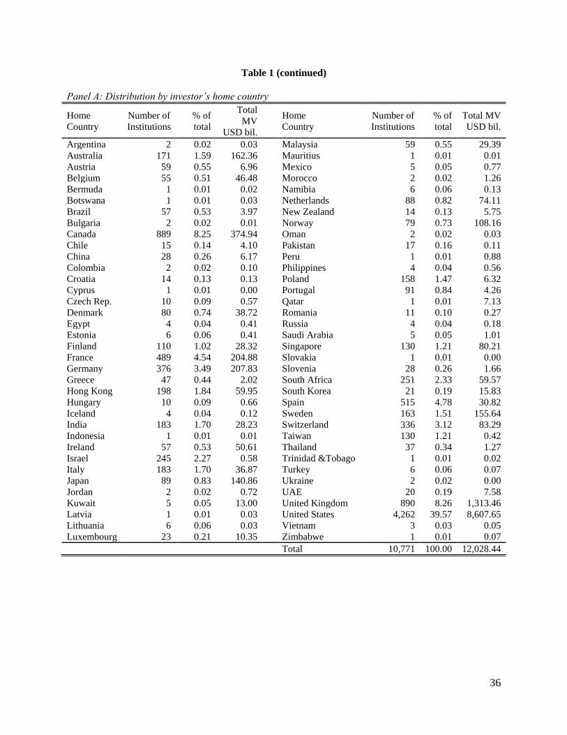
Table 1 presents the sample distribution by the investor’s home country (Panel A) and by

target country (Panel B). Panel A shows that virtually all parts of the world are represented in our

sample, with wide representation from developed and emerging markets. Altogether, the sample

consists of 10,771 institutional investors. About 40% of the sample, 4,262 institutions, are

institutional investors from the US, followed by 890 institutions from the United Kingdom, and

889 from Canada. Other less researched countries are also represented in the sample; for

3 We also use the security’s country of domicile as an alternative way to define “home country”. The results are

unaffected by the definition.

11

example, the sample includes 251 institutions from South Africa, 183 from India, 130 from

Taiwan, and 57 from Brazil. Panel A also shows time-series median of the total value of assets

under management (in billions of US dollars) by all institutional investors domiciled in each

country. The total market value of assets of US institutional investors is $8.607 trillion US

dollars, which is the highest among all institutions in our sample, followed by $1.313 trillion US

dollars for UK investors, and by $375 billion US dollars for Canadian investors.

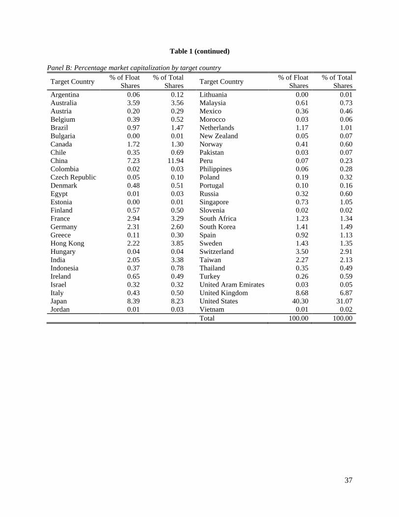
Panel B shows each target country’s average share of the world market capitalization

during the time period of our study. The percentage of float shares is calculated by dividing the

total market value of investable, or “float” shares of each country by the aggregate market value

of float shares from our sample countries. The percentage of total shares is calculated by dividing

the total market capitalization of each country by the aggregate market capitalization of every

country in our sample. Total market value and total float share values are from Worldscope as of

the end of 2012. Panel B shows that about 40% of the investable world market capitalization

consists of the securities listed in the US market, followed by almost nine percent in United

Kingdom (8.68%), 8.39% in Japan, and 7.23% in China.

[Insert Table 1 here]

4. Methodology

4.1. Performance analysis at the institutional portfolio level

4.1.1. Portfolio performance measure

To test our hypothesis, we first conduct the analysis at the institution’s overall portfolio

level, using portfolio excess return as a measure of performance. Portfolio excess return, Reti,q, is

calculated as the value-weighted return of the securities held by the institution over a given

12

quarter less the global risk-free rate over the same quarter, obtained from Kenneth French’s data

library.4 Value-weighted quarterly returns are compounded using split-adjusted monthly returns

for three consecutive months surrounding the reporting month (Rett-1, t+1).5 We analyze whether

institutional investors who concentrate their portfolios in a few markets and industries achieve

better portfolio performance than globally/industry diversified investors.

We examine three measures of portfolio concentration: home bias, foreign concentration,

and global industry concentration (each measure discussed below). We conjecture that

coefficients on these portfolio concentration measures should take a positive sign if institutional

investors with more concentrated portfolios outperform investors with more diversified

portfolios due to information advantage from the initial information asymmetry and

specialization in a given set of securities. In all of our regressions we also control for the

institution’s portfolio size and systematic risk. Portfolio Size is measured as the natural logarithm

of the institution’s market value of equity in quarter q. Market Premium is the market return in

quarter q less the global risk-free rate in the same quarter. Market return equals to global market

return, obtained from Kenneth French’s data library, when evaluating overall portfolio

performance and it equals to each country’s equally weighted market return, based on securities’

4 Kenneth French’s Data Library: http://mba.tuck.dartmouth.edu/pages/faculty/ken.french/data_library.html.

5 The portfolio return is the return to the hypothetical portfolio that consists of the securities reported by the

institution. We compute the return to portfolio of securities leading up to the reporting month (month t) from two

months prior (Rett-2, t) and three months following the reporting month (Rett+1, t+3) as a robustness check. We believe

that the way we compute the hypothetical returns eliminates survivorship bias from the sample.

13

return data for that country, when evaluating performance in the target country (home or

foreign). Securities’ return data are obtained from FactSet.

We also examine whether the results on concentration measures hold once we control for

additional dimensions of systematic risk. We do this by including size (SMBq), value (HMLq),

and momentum (UMDq) global factors in the analysis. These factors have been used in prior

studies to explain the variation in international stock returns (see Fama and French, 2010, 2012;

Ferreira, Matos, and Pereira, 2009; Hou, Karolyi, and Kho, 2011). SMBq is the difference

between the returns on a diversified portfolio of small and large stocks over quarter q; HMLq is

the difference between the returns of value and growth stocks over quarter q; and UMDq is the

difference between the returns on winners and losers over quarter q. Data on the global factors

are also from Kenneth French’s data library.

4.1.2. Portfolio concentration measures

This section describes three portfolio concentration measures used in this study: Home

Bias, Foreign Concentration, and Global Industry Concentration. Appendix provides numerical

examples of each measure.

Home Bias

For each institutional investor, we calculate portfolio Home Bias as the difference

between the actual portfolio weight of the institution’s holdings in the home country and the

expected portfolio allocation to the home country. To calculate the actual portfolio weight of the

home country, we compute a quarterly portfolio weight of stock holdings in the home country

14

divided by the total value of the institution’s aggregate portfolio in a given quarter. Actual

portfolio weight of the home country, Home Weight, is formally defined as:

, ,

, ,

, i I q

i J q

i q

I J

pHome Weight

p

(1)

where pi,I,q is the total market value of all securities held by institution i in the home country I in

quarter q. The denominator is the total value of institution i’s aggregate portfolio invested in J

countries, including the investor’s home country I, in quarter q.

Expected portfolio allocation to investor i’s home country in quarter q is based on

country I’s share of the world market capitalization reported by WorldScope.6 According to the

traditional asset pricing theory, the portion of the portfolio invested in a given country should

equal to the country’s world capitalization weight. For example, since US market float

capitalization accounts for about 40% (Panel B in Table 1) of the aggregate world market

capitalization during our sample period, investors worldwide should hold 40% of their overall

portfolios in US stocks and invest the remaining 60% in the securities of other countries.

Formally, Home Bias for institutional investor i in quarter q, is calculated as:

,

, ,

,

I q

i q i q

J q

I J

MVHome Bias Home Weight

MV

, (2)

6 We use both the securities’ total market capitalization and “float based” or “investable” market capitalization to

calculate the expected allocation. Since float based capitalization is typically used in international studies, we report

the results using float based computation.

15

where Home Weighti,q is defined in Eq. (1), MVI,q is the total market value of institution i’s home

country I in quarter q, and the denominator of the second term on the right-hand side is the

aggregate world market capitalization in quarter q. Home Bias measure captures

under/overweighting of institution i’s home country I relative to the share of country I in the

aggregate world market capitalization. Higher Home Bias value indicates that the investor’s

portfolio is more overweighted in the investor’s home country.

Foreign Concentration

We then compute Foreign Concentration measure for each institutional investor. In

contrast to Home Bias, which indicates the under- or overweight of the institution’s home

country in the institution’s aggregate portfolio, Foreign Concentration measure indicates

whether or not the investor’s foreign share of the portfolio is well-diversified across foreign

markets. The traditional asset pricing theory suggests that portfolio weight allocated to a given

foreign country should equal to that country’s share of the world market capitalization. In

practice, investors worldwide tend to concentrate their portfolios only in a few foreign markets.

We conjecture that investors may choose to concentrate their holdings in a few foreign markets if

learning about a narrow set of assets generates information advantage. If there is information

advantage to focusing and specializing in a few foreign markets, then portfolios concentrated in a

few foreign markets should outperform portfolios that are well-diversified across foreign

markets. In contrast, the traditional asset pricing theory predicts that well-diversified portfolios

outperform concentrated portfolios.

To calculate Foreign Concentration measure, we first compute each institution’s Foreign

Bias in each foreign country that is available for investment, and then aggregate Foreign Bias

16

across all countries, excluding the institution’s home country. We take the following two steps to

calculate Foreign Bias. First, we calculate Foreign Weight as:

, ,

, ,

, ,

i J q

i J q

i J q

I J

pForeign Weight

p

, (3)

where pi,J,q is the total market value of the securities held by institution i, listed in country J in

quarter q. The denominator is the total market value of the securities held by institution i in J

countries, excluding the investor’s home country I in quarter q.7

We then calculate Foreign Bias, similar to the Home Bias in Eq. (2), as follows:

,

, , , ,

,

J q

i J q i J q

J q

I J

MVForeign Bias Foreign Weight

MV

, (4)

where Foreign Weighti,J,q is the actual allocation to the foreign market J in investor i’s portfolio

in quarter q, calculated in Eq. (3), and the second term on the right-hand side is the expected

portfolio allocation to country J, calculated according to the country’s world capitalization

7 Since the extant literature documents a large home bias in the investors’ portfolios, scaling by the total value of

foreign holdings rather than by the total value of overall portfolio captures the investor’s concentration in the foreign

markets more precisely. We believe that computing foreign bias without the home market is an improvement to the

way prior literature (e.g., Chan, Covrig, and Ng, 2005) computes foreign underdiversification because it allows us to

focus on the foreign country weights independent of home bias. Foreign bias computed including the home market

results in a foreign bias measure that is highly correlated with home bias. For robustness, we also compute Global

Concentration measure, which includes home country I and uses total portfolio weights. The Global Concentration

is highly correlated with home bias, and produces results quantitatively similar to the home bias results. Therefore,

we omit the regressions with Global Concentration from the paper for brevity.

17

weight, excluding investor i’s home country I. This Foreign Bias measure indicates whether the

investor over/underweights country J in quarter q relative to country J’s share of the world

market capitalization in quarter q, excluding the investor’s home country I. The foreign bias

measure is computed for all available target markets, even if investor i’s actual investment in

country J is zero.8

To estimate the degree of investor’s concentration in foreign markets, we calculate

Foreign Concentration by aggregating Foreign Bias from Eq. (4) across all available foreign

countries. The resulting Foreign Concentration measure is:

, ,

,

2

i J q

i q

I J

Foreign BiasForeign Concentration

. (5)

This measure can be interpreted as the fraction of the institution’s foreign holdings that should be

reallocated across foreign countries to achieve perfect foreign diversification. It is zero for

portfolios with allocations in foreign countries made exactly in line with countries’ market

capitalization weights, thus, for perfectly diversified portfolios. A measure greater than zero

indicates the portfolio is not perfectly diversified across foreign countries but instead is

concentrated in a few foreign countries. The upper bound of the measure is 1.0, meaning that

100% of the institution’s foreign holdings should be reallocated across foreign markets.9 The

8 We define the set of “available” target markets based on a positive float weight according to WorldScope.

Additionally, we require a presence of at least one foreign institutional investor before including target market J in

our analysis.

9 Theoretically, the upper bound on Foreign Concentration approaches 1. In our sample all target markets have non-

zero market capitalization (the smallest float-based percentage share is 0.0017% for Bulgaria), so an investor with

18

Appendix provides some simple numeric examples of Foreign Bias and Foreign Concentration

calculations and interpretations.

Global Industry Concentration

In addition to home and foreign markets portfolio concentrations, we examine portfolio

industry concentration. Kacperczyk, Sialm, and Zheng (2005) document, using a sample of US

mutual funds, that industry concentrated portfolios outperform industry diversified portfolios.

They suggest that managers of industry concentrated funds possess some information advantage

about industry performance. Extending their study, we examine whether industry concentration

enhances investors’ performance in the sample of global institutional investors. To estimate

portfolio industry concentration, we calculate Global Industry Concentration as the aggregate of

the differences between institutions’ actual and expected allocations to a given industry. Similar

to the calculation of the Foreign Concentration measure, we first calculate industry bias of each

institutional investor in each available industry, defined based on the two-digit industry SIC

code. We then aggregate these individual industry biases into one comprehensive portfolio level

concentration measure. Formally, the Global Industry Bias is calculated as:

, , ,

, ,

, , ,

i SIC q SIC q

i SIC q

i SIC q SIC q

SIC SIC

p MVGlobal Industry Bias

p MV

, (6)

where pi,SIC,q is the market value of all securities held by institution i in quarter q that belong to a

two-digit SIC industry. We scale this value by the total market value of institution’s holdings

all his holdings in a very small market will have a measure close to 1 but not actually 1 (e.g., an investor whose

entire foreign portfolio is invested in Bulgaria needs to reallocate 99.9983% of his investment).

19

across all industries in quarter q. If institution i has zero investment in the two-digit SIC in

quarter q, the first term on the right-hand side is zero. The second term on the right-hand side is

the expected allocation to the two-digit SIC industry, calculated as the market value of all

securities in a given industry in quarter q, divided by the total market value of securities across

all industries in quarter q, i.e., the total world market capitalization in quarter q. We then

aggregate the industry biases for each institution i in each industry SIC and calculate Global

Industry Concentration as:

, ,

,

2

i SIC q

i q

SIC

Global Industry BiasGlobal Industry Concentration . (7)

This measure can be interpreted as the fraction of the institution’s holdings that should be

reallocated across industries to achieve perfect global industry diversification. It is zero for an

investor with portfolio allocations in industries made exactly in line with industries’ market

capitalization weights, thus, for a perfectly diversified portfolio. A measure greater than zero

indicates the portfolio is not perfectly diversified across industries. The upper bound of the

measure is 1.0 which suggests that 100% of the portfolio has to be reallocated to achieve perfect

industry diversification (see footnote 9). The Appendix also provides some simple numeric

examples of Global Industry Concentration calculations and interpretations.

4.2. Performance analysis at the target market level

In addition to the overall portfolio performance, we examine the institution’s

performance in the part of the portfolio concentrated in a given target market. According to the

information advantage theory, investors benefit from specializing and concentrating their

holdings in a few set of securities. We analyze if the investor’s concentration in a given country

20

enhances the investor’s performance in that country’s securities. In other words, we examine

whether investors choose to concentrate their holdings in certain countries because they have

some information advantage about securities’ payoffs in these countries, resulting in higher

excess returns in the investments in the target market. This analysis complements the aggregate

portfolio analysis and addresses the possibility that investors may achieve above-benchmark

performance in countries where they concentrate their holdings, but the superior performance

may not be evident when overall portfolio performance is considered. To test whether

concentration in a given country enhances the investor’s performance in that country’s securities,

we analyze if higher portfolio weight in country J enhances institution i’s performance in country

J’s securities. In addition, we analyze if high industry concentration in country J enhances

institution i’s performance in country J’s securities.

For these analyses, we compute excess returns for each institution i in each country J in

which institution i has holdings. The quarterly excess return in target country J for each

institutional investor i, Reti,J,q, is calculated as value-weighted return on the securities held by

institution i in country J in quarter q, less the global risk-free rate over the same time period.10

The country concentration measure, Country Weighti,J.q, equals to Home Weight (Eq. (1)) when

target country J is the investor’s home country and equals to Foreign Weight (Eq. (3)) when

10 Similar to the portfolio return, the market J return is the return to the hypothetical portfolio that consists of the

securities reported by the institution. We compute the return to market J securities leading up to the reporting month

and three months following the reporting month as a robustness check. We believe that the way we compute the

hypothetical returns eliminates survivorship bias from the sample.

21

target country J is a foreign country. The industry concentration measure in a given country is

calculated as described below.

We start by calculating Country Industry Bias as the difference between the actual

allocation of the institution’s holdings invested in a given industry in each country and the

expected allocation to the industry in that country:

, , , , ,

, , ,

, , , , ,

i SIC J q SIC J q

i SIC J q

i SIC J q SIC J q

SIC SIC

p MVCountry Industry Bias

p MV

, (8)

where pi,SIC,J,q is the total market value of investor i’s holdings in two-digit industry SIC in

country J in quarter q, and MVSIC,J,q is the total market value of all securities classified in two-

digit industry SIC in country J in quarter q. The denominator of the first term on the right-hand

side is the total market value of institution i’s portfolio in quarter q invested in country J and the

denominator of the second term on the right-hand side is the total market capitalization of

country J in quarter q. Following methodology described in Section 4.1.3, the Country Industry

Concentration measure is calculated as:

, , ,

, ,

2

i SIC J q

i J q

SIC

Country Industry BiasCountry Industry Concentration .

(9)

The interpretation of Country Industry Concentration is similar to that of Global Industry

Concentration. It is the fraction of institution i’s portfolio that should be reallocated across

different industries in country J to achieve perfect industry diversification within country J.

4.3. Country and industry concentration measures: Summary statistics

22

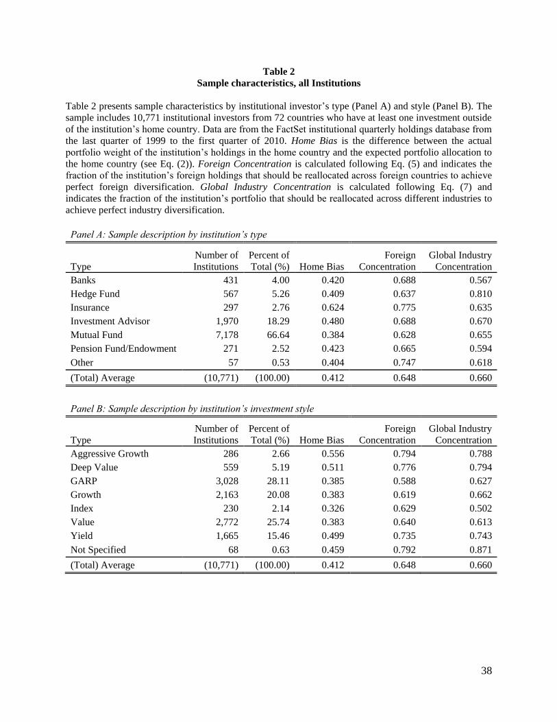
Table 2 presents average values of Home Bias, Foreign Concentration, and Global

Industry Concentration for the sample institutions. Panel A shows the measures by institution’s

type and Panel B by institution’s style. As far as institution’s type, mutual funds are the most

represented category (66.64% of the sample), followed by investment advisors (18.29%) and

hedge funds (5.26%). All types of institutions overweight the home market quite heavily, with

the average Home Bias measure of 0.412. Insurance funds overweight the home market the most

(Home Bias= 0.624), while mutual funds overweight the home market the least (Home Bias=

0.384). Similarly, all institutions are heavily concentrated in a few foreign markets. The average

Foreign Concentration measure of 0.648 indicates that almost 65% of institutions’ foreign

holdings should be reallocated across foreign markets to achieve perfect diversification. Again,

out of all institutions’ types, insurance funds are the most concentrated in the foreign markets

(Foreign Concentration=0.775), and mutual funds are the least concentrated in the foreign

markets (Foreign Concentration=0.628). All institutional investors are also heavily industry

concentrated. The sample average Global Industry Concentration is 0.660 and ranges from 0.594

for pension funds/endowments to 0.810 for hedge funds. The measure shows that, on average,

over 60% of the institutions’ portfolios in a given country should be reallocated across different

industries.

Panel B breaks the sample by the investment style and shows that 28% of the institutions

follow GARP (Growth At Reasonable Price) investment style, almost 26% label themselves as

Value funds, and 20% follow Growth investment strategy. The Home Bias value ranges from

0.326 for Index funds to 0.556 for Aggressive Growth funds. Foreign Concentration is also the

highest for the Aggressive Growth (0.794) and is the lowest for the GARP funds (0.588). All

23

investment style categories are heavily industry concentrated, with the Index funds having the

lowest Global Industry Concentration measure of 0.502, and Deep Value the highest of 0.794.


Overall, sample description in Table 2 shows that institutions of different types and with

different investment styles are heavily concentrated in home markets’ securities and in a few

industries. The parts of the portfolios that are allocated to foreign countries are heavily

concentrated in a few foreign countries. This evidence on a wide range of institutional investors

worldwide complements prior evidence documented in a single- or a few-countries’ studies for

selected types of institutional investors (e.g., mutual funds).

5. Results

5.1. Portfolio level performance

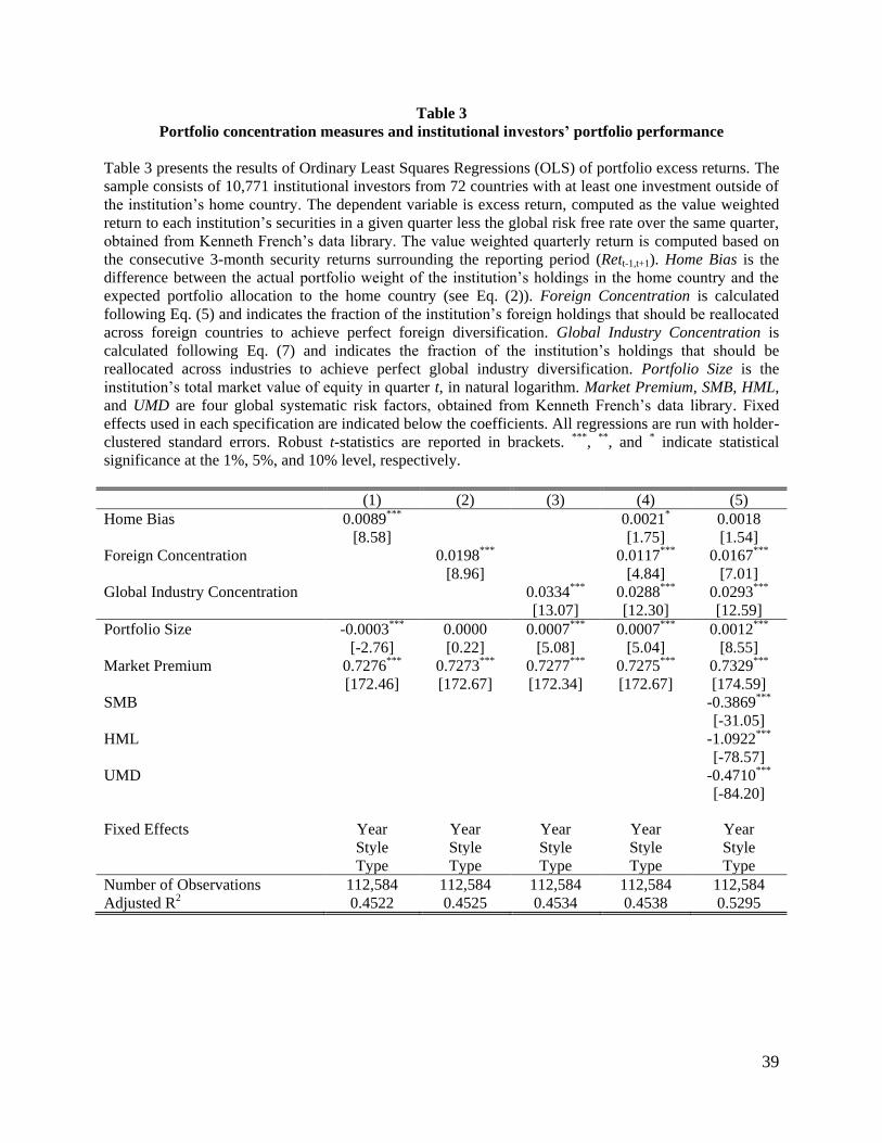
Table 3 presents the results of ordinary least squares (OLS) regressions of institution’s

excess portfolio returns on portfolio concentration measures.


In specifications 1, 2, and 3, we examine individually our main explanatory variables: Home

Bias, Foreign Concentration, and Global Industry Concentration, respectively. The coefficients

on all three portfolio concentration measures are positive and significant at the 1% level,

suggesting that institutional investors who concentrate their holdings in home country and in a

few foreign countries and industries achieve better portfolio performance. In specification 4, we

include all three measures of portfolio concentration simultaneously and show that the

coefficients on all three portfolio concentration measures remain positive, even though the

statistical significance of Home Bias measure drops to the 10% level. All four models control for

24

the size of the institution’s portfolio and the global market premium and include year,

institution’s style and type fixed effects. To adjust for additional dimensions of systematic risk,

in addition to the global market premium, we follow Fama and French (2012) and add global risk

factors (SMB, HML, and UMD) in specification 5. The coefficients on Foreign Concentration

and Global Industry Concentration remain positive and highly significant at the 1% level;

however, the statistical significance of Home Bias drops below conventional levels.11

Overall, the results presented in Table 3 indicate that portfolios that are more

concentrated in a few countries and industries perform better than portfolios that are more

diversified across countries and industries. The result is particularly strong for portfolio

concentration in foreign markets and industries. These findings suggest that investors have some

information advantage when forming concentrated portfolios, which results in better portfolio

performance at risk adjusted basis.

5.2. Performance in the target market

In this section, we examine performance of the part of the institutional investor’s

portfolio concentrated in a given target market. We hypothesize that if portfolio concentration is

based on information advantage, the investor’s concentration in a given country should result in

better performance in that country’s securities. We examine the relation between the

11 However, in unreported results that replicate analysis of specification 1 with the four factor model, home bias is

positive and statistically significant. This is true across the robustness checks in this paper. Home bias is consistently

positive determinant of performance. However, when included simultaneously with the other two concentration

measures, home bias in some cases loses its significance.

25

performance of each institutional investor in the target market and our three portfolio

concentration measures. To measure the performance of each institutional investor in the target

market we calculate excess returns for each institution i in each country J in which institution i

has holdings, as defined in Section 4.2.

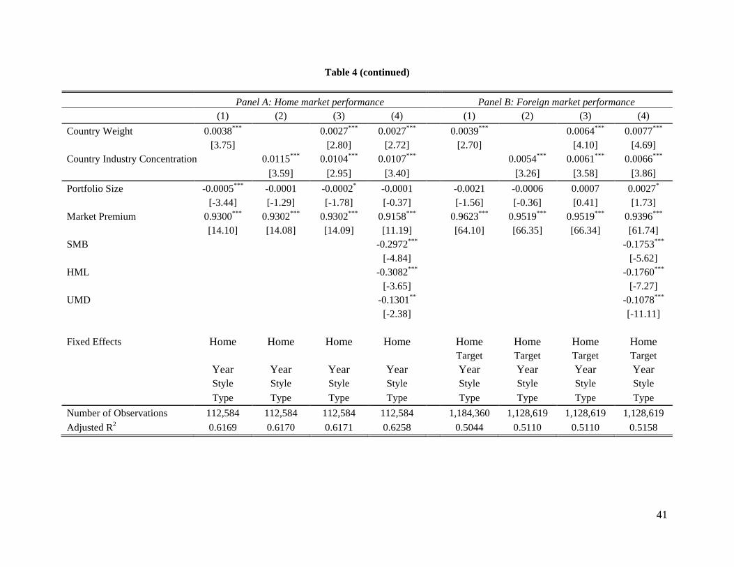
Table 4 reports the results. Panel A presents findings for the institution’s performance in

the institution’s home market, where the variable Country Weight, equals to Home Weight (Eq.

(1)). Panel B presents the results for investments outside of the institution’s domicile country,

where Country Weight equals to Foreign Weight (Eq. (3)). The coefficient on Country Weight

should carry a positive sign if portfolio concentration in any particular target market (either

foreign or home) improves the investor’s performance in that market. In addition to target market

concentration, we examine the effect of industry concentration in a given target market by

including Country Industry Concentration variable defined in Section 4.2. If investors

concentrate in a few industries in a given target market because of information advantage, the

coefficient on Country Industry Concentration should be positive. Similar to the analysis

presented in Table 3, we perform panel OLS regressions and first include country (specification

1) and industry (specification 2) concentration measures individually and then combine two

measures in specification 3. In all specifications we control for portfolio size and the target

country J market premium. In specification 4 we also add size, value, and momentum global risk

factors. In addition to year, style, and type fixed effects, we also include country fixed effects

(home country in Panel A; home and foreign country in Panel B) to account for any differences

in legal environment, investor protection, and economic development across countries.

The results presented in Tables 4 show that Country Weight is positive and highly

significant in all specifications, indicating that increasing portfolio concentration in a given

26

target market (either home or foreign) results in better performance in the target market’s

securities. The result holds when we include year and country fixed effects and when we include

fixed effects for the institutional investor’s style and type.


In addition to country concentration, we examine the effect of Country Industry

Concentration (Eq. (9)) and expect a positive sign on this variable if concentrating in a given

industry improves the investor’s performance. Extending prior findings for the US market in

Kacperczyk, Sialm, and Zheng (2005), we show that industry concentration enhances

performance of institutional investors globally. The coefficient on Country Industry

Concentration is positive and highly significant in all specifications suggesting that institutional

investors who overweight certain industries in their home (Panel A) and foreign (Panel B)

countries, as opposed to diversifying across industries, possess information advantage in these

industries as they achieve better performance.

Again, the results are robust to including controls for year, home, and target country fixed

effects, institution’s style and type, and Fama and French (2012) global risk factors. These

results provide additional support for the findings presented above that concentrated portfolios

are optimal due to information advantage from economies of scale and specialization.

5.3. Robustness Checks

5.3.1 Alternative measure of abnormal returns

In this section, we examine an alternative measure of the dependent variable used in the

portfolio level performance analysis. Instead of using portfolio excess return as in Table 3, we

27

measure abnormal return (alpha (i)) of the institutional investor’s portfolio from the following

regression as per Fama and French (2012):

, ,i q i i q i q q q i qRet MP SMB HML UMD , (10)

where Reti,q is the portfolio excess return as described in section 4.1, MPq is the global market

premium, SMBq is the global size factor, HMLq is the global book-to-market factor, and UMDq is

the global momentum factor, all obtained from Kenneth French’s data library.

Similar to the analysis presented in Table 3, we examine the relation between portfolio

performance, measured as alpha from Eq. (10)12

, and our three portfolio concentration measures:

Home Bias, Foreign Concentration, and Global Industry Concentration. Portfolio Size,

measured as the institution’s total market value of equity in quarter q is used as a control

variable. We also include year and institution’s style and type fixed effects. The results are

presented in Table 5.


12 In these robustness checks, we have explored several windows in measuring portfolios’ rolling alphas. The

shortest time period in estimating alpha is two years (eight quarters) and the longest time period is over 10 years (40

quarters). Because we are dealing with quarterly observations of excess performance, the shorter time periods’

alphas have a high variance (although the mean and median are near zero, as expected). The accuracy of the alpha

estimation improves when we use longer windows and therefore the robustness checks reported in this paper include

alphas that are estimated using all available observations for each institution. The coefficients on portfolio

concentration measures are, however, similar if we use alpha from these various rolling windows as the dependent

variable.

28

Similar to the analysis described above, we first examine the effect of Home Bias,

Foreign Concentration, and Global Industry Concentration individually (specifications 1, 2, and

3, respectively). In specification 4 we combine all three portfolio concentration measures.

Results for this alternative measure of abnormal performance are consistent with those presented

in Table 3. All three portfolio concentration measures are positive and significant at the 1% level

when they are included separately. The coefficient on Home Bias remains positive but loses

statistical significance once all concentration measures are examined simultaneously

(specification 4). This analysis confirms our results with an alternative portfolio performance

measure.

5.3.2. Mutual funds vs. other types of institutional investors

The sample examined in this study consists of different types of institutional investors;

however, mutual funds dominate the sample. While we control for the institution’s type in all our

regressions presented above, in this section we perform the analysis separately for mutual funds

and for all other types of institutional investors. The purpose of this analysis is to examine

whether the positive relation between portfolio concentration and performance is driven by

mutual funds and cannot be generalized to other types of intuitional investors. Table 6 presents

the results of this analysis and replicates Tables 3 and 4 separately for mutual funds (MF) and for

all other institutional investors (non-MF). Panel A presents the results of overall portfolio excess

returns. Panels B and C present the results of excess returns in the home and foreign target

markets, respectively. Similar to our prior analysis, the regressions are run by including portfolio

concentration measures first individually and then simultaneously.


29

Overall, the results hold for mutual funds and for other types of institutional investors. In

general, the evidence is consistent with the hypothesis that portfolio concentration in country and

industry is beneficial for the performance of mutual funds and of other types of institutional

investors.

5.3.3. Performance of non-US institutional investors

Another possibility is that the positive relation between portfolio concentration and

investors’ performance documented above is driven by US investors. Institutional investors from

the US comprise 40% of the sample. It is possible that only US investors benefit from

concentrated investment strategies and information advantage due to better development of

financial markets and other factors. Even though we control for country fixed effects in our prior

regressions, in Table 7, we report the results of portfolio level performance (Panel A) and

performance in the home (Panel B) and foreign (Panel C) target markets for the sample of non-

US institutional investors. Results for non-US institutional investors are similar to the results for

the entire sample of institutional investors. Portfolio concentration across industry or target

country improves the performance of non-US institutional investors. These results confirm that

the findings for country and industry concentration are not driven by the largest group of the

investors (the US investors). These findings suggest that portfolio concentration across countries

and industries results in better performance of institutional investors worldwide.


6. Conclusion

30

Prior empirical studies document that investors often pursue concentrated rather than

diversified investment strategies. These findings refute the implications of traditional asset

pricing theory that diversified portfolios are optimal and suggest that investors do not take

advantage of international diversification opportunities. More recent theoretical studies (e.g.,

Gehrig 1993; Van Nieuwerburgh and Veldkamp 2009, 2010) argue that portfolios can be

underdiversified but optimal if they are formed on information advantage.

Using data on security holdings of 10,771 institutional investors from 72 different

countries, we test whether concentrated investment strategies result in superior abnormal returns

to institutional investors worldwide. We examine three measures of portfolio concentration:

home bias, foreign country concentration, and industry concentration; and we use two measures

of institutional investors’ performance: overall portfolio performance and performance of the

part of the portfolio invested in a target country. We find strong support for the information

advantage theory with respect to all concentration measures. Results show that home country,

foreign country, and industry focus lead to higher abnormal returns of institutional investors

worldwide.

We contribute to the existing literature in several ways. First, we analyze the extensive

dataset of security holdings by global institutional investors and compute several different

measures of portfolio concentration and performance of institutional investors worldwide.

Second, we introduce a method of computing portfolio concentration that is intuitive and

straightforward and can be used to calculate portfolio concentration across other different

dimensions. Finally, we analyze the performance of the overall portfolio and the part of the

portfolio invested in a target country, examining whether portfolio concentration in a given target

market or in a given industry results in better aggregate portfolio performance or in better

31

performance of the part of the portfolio that is more likely to benefit from the information

advantage. Our study contributes to the literature on home bias and international

underdiversification and extends the existing literature on industry concentration of US mutual

funds.

32

References

Bhargava, R., Gallo, J., Swanson, P., 2001. The performance, asset allocation, and investment

style of international equity managers, Review of Quantitative Finance and Accounting

17, 377-395.

Brands, S., Brown, S., Gallagher, D., 2005. Portfolio concentration and investment manager

performance, International Review of Finance 5, 149-174.

Chan, K., Covrig, V., Ng, L., 2005. What determines the domestic bias and foreign bias?

Evidence from Mutual Fund Equity Allocations Worldwide, Journal of Finance 60, 1495-

1534.

Choe, H., Kho, B., Stulz, R., 2005. Do domestic investors have an edge? The trading experience

of foreign investors in Korea, Review of Financial Studies 18, 795-829.

Coval, J., Moskowitz, T., 2001. The geography of investment: Informed trading and asset prices,

Journal of Political Economy 109, 811-841.

Dvořák, T., 2005. Do domestic investors have an information advantage? Evidence from

Indonesia, Journal of Finance 60, 817-839.

Fama, E., French, K., 2010. Luck versus Skill in the Cross-Section of Mutual Fund Returns,

Journal of Finance 65, 1915-1947.

Fama, E., French, K., 2012. Size, value and momentum in international stock returns, Journal of

Financial Economics 105, 457-472.

Ferreira, M., Matos, P., 2008. The colors of investors’ money: The role of institutional investors

around the world, Journal of Financial Economics 88, 499-533.

Ferreira, M., Matos, P., Pereira, J., 2009. Do foreigners know better? A comparison of the

performance of local and foreign mutual fund managers, Unpublished working Paper,

Universidade Nova de Lisboa, University of Southern California, and ISCTE Business

School.

French, K., Poterba, J., 1991. Investor diversification and international equity markets, American

Economic Review 81, 222-226.

Gehrig, T., 1993. An information based explanation of the domestic bias in international equity

investment, The Scandinavian Journal of Economics 95, 97-109.

Grauer, R., Hakansson, N., 1987. Gains from International Diversification: 1968–85 Returns on

Portfolios of Stocks and Bonds, Journal of Finance 42, 721-739.

33

Grubel, H., 1968. Internationally Diversified Portfolios: Welfare Gains and Capital Flows,

American Economic Review 58, 1299-1314.

Hau, H., 2001. Location matters: An examination of trading profits, Journal of Finance 56, 1959-

1983.

Hou, K., Karolyi., G. A., Kho, B. C., 2011. What Factors Drive Global Stock Returns? Review

of Financial Studies 24, 2527-2574.

Ivković, Z., Weisbenner, S., 2005. Local does as local is: Information content of the geography

of individual investors' common stock investments, Journal of Finance 60, 267-306.

Kacperczyk, M, Sialm, C., Zheng, L., 2005. On the industry concentration of actively managed

equity mutual funds, Journal of Finance 60, 1983-2011.

Karolyi, A., Stulz, R., 2003. Are financial assets priced locally or globally?, Handbook of the

Economics of Finance 1, 975-1020.

Levy, A., Livingston, M., 1995. The gains from diversification reconsidered: transaction costs

and superior information, Financial Markets, Institutions, and Instruments 4, 1-60.

Levy, H., Sarnat, M., 1970. International diversification of investment portfolios, The American

Economic Review 60, 668-675.

Lewis, K., 1999. Trying to explain home bias in equities and consumption, Journal of Economic

Literature 37, 571-608.

Li, D., Moshirian, F., Pham, P., Zein, J., 2006. When financial institutions are large shareholders:

The role of macro corporate governance environments, Journal of Finance 61, 2975-

3007.

Markowitz, H., 1952. Portfolio selection, Journal of Finance 7, 77-91.

Merton, R., 1987. A Simple Model of Capital Market Equilibrium with Incomplete Information,

Journal of Finance 42, 483–510.

Nanda, V., Wang, Z., Zheng, L., 2004. Family values and the star phenomenon, Review of

Financial Studies 17, 667-698.

Shukla, R., van Inwegen, G., 1995. Do locals perform better than foreigners? An analysis of UK

and US mutual fund managers, Journal of Economics and Business 47, 241-254.

Thomas, C., Warnock, F., Wongswan, J., 2006. The performance of international portfolios,

FRB International Finance Discussion Paper No. 817.

34

Van Nieuwerburgh, S., Veldkamp, L., 2009. Information immobility and the home bias puzzle,

Journal of Finance 64, 1187-1215.

Van Nieuwerburgh, S., Veldkamp, L., 2010, Information acquisition and portfolio under-

diversification, Review of Economic Studies 77, 779-805

35

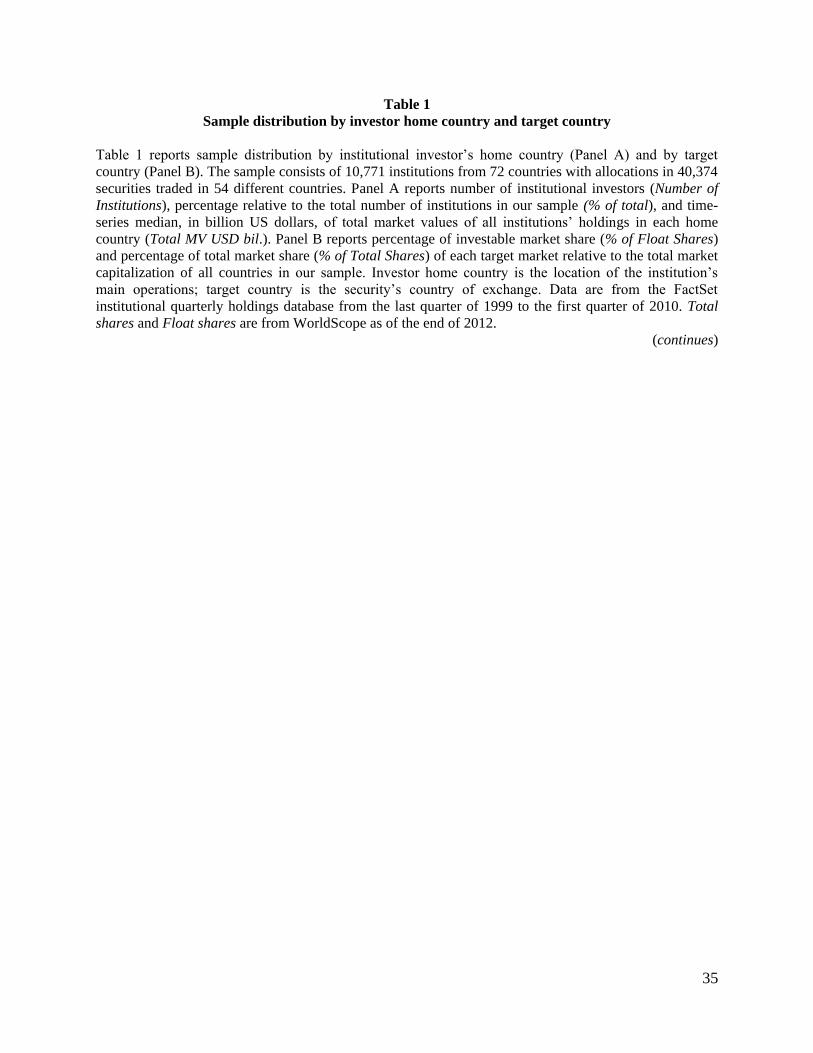
Table 1

Sample distribution by investor home country and target country

Table 1 reports sample distribution by institutional investor’s home country (Panel A) and by target

country (Panel B). The sample consists of 10,771 institutions from 72 countries with allocations in 40,374

securities traded in 54 different countries. Panel A reports number of institutional investors (Number of

Institutions), percentage relative to the total number of institutions in our sample (% of total), and time-

series median, in billion US dollars, of total market values of all institutions’ holdings in each home

country (Total MV USD bil.). Panel B reports percentage of investable market share (% of Float Shares)

and percentage of total market share (% of Total Shares) of each target market relative to the total market

capitalization of all countries in our sample. Investor home country is the location of the institution’s

main operations; target country is the security’s country of exchange. Data are from the FactSet

institutional quarterly holdings database from the last quarter of 1999 to the first quarter of 2010. Total

shares and Float shares are from WorldScope as of the end of 2012.

(continues)

36

Table 1 (continued)

Panel A: Distribution by investor’s home country

Home

Country

Number of

Institutions

% of

total

Total

MV

USD bil.

Home

Country

Number of

Institutions

% of

total

Total MV

USD bil.

Argentina 2 0.02 0.03 Malaysia 59 0.55 29.39

Australia 171 1.59 162.36 Mauritius 1 0.01 0.01

Austria 59 0.55 6.96 Mexico 5 0.05 0.77

Belgium 55 0.51 46.48 Morocco 2 0.02 1.26

Bermuda 1 0.01 0.02 Namibia 6 0.06 0.13

Botswana 1 0.01 0.03 Netherlands 88 0.82 74.11

Brazil 57 0.53 3.97 New Zealand 14 0.13 5.75

Bulgaria 2 0.02 0.01 Norway 79 0.73 108.16

Canada 889 8.25 374.94 Oman 2 0.02 0.03

Chile 15 0.14 4.10 Pakistan 17 0.16 0.11

China 28 0.26 6.17 Peru 1 0.01 0.88

Colombia 2 0.02 0.10 Philippines 4 0.04 0.56

Croatia 14 0.13 0.13 Poland 158 1.47 6.32

Cyprus 1 0.01 0.00 Portugal 91 0.84 4.26

Czech Rep. 10 0.09 0.57 Qatar 1 0.01 7.13

Denmark 80 0.74 38.72 Romania 11 0.10 0.27

Egypt 4 0.04 0.41 Russia 4 0.04 0.18

Estonia 6 0.06 0.41 Saudi Arabia 5 0.05 1.01

Finland 110 1.02 28.32 Singapore 130 1.21 80.21

France 489 4.54 204.88 Slovakia 1 0.01 0.00

Germany 376 3.49 207.83 Slovenia 28 0.26 1.66

Greece 47 0.44 2.02 South Africa 251 2.33 59.57

Hong Kong 198 1.84 59.95 South Korea 21 0.19 15.83

Hungary 10 0.09 0.66 Spain 515 4.78 30.82

Iceland 4 0.04 0.12 Sweden 163 1.51 155.64

India 183 1.70 28.23 Switzerland 336 3.12 83.29

Indonesia 1 0.01 0.01 Taiwan 130 1.21 0.42

Ireland 57 0.53 50.61 Thailand 37 0.34 1.27

Israel 245 2.27 0.58 Trinidad &Tobago 1 0.01 0.02

Italy 183 1.70 36.87 Turkey 6 0.06 0.07

Japan 89 0.83 140.86 Ukraine 2 0.02 0.00

Jordan 2 0.02 0.72 UAE 20 0.19 7.58

Kuwait 5 0.05 13.00 United Kingdom 890 8.26 1,313.46

Latvia 1 0.01 0.03 United States 4,262 39.57 8,607.65

Lithuania 6 0.06 0.03 Vietnam 3 0.03 0.05

Luxembourg 23 0.21 10.35 Zimbabwe 1 0.01 0.07

Total 10,771 100.00 12,028.44

37

Table 1 (continued)

Panel B: Percentage market capitalization by target country

Target Country % of Float

Shares

% of Total

Shares Target Country

% of Float

Shares

% of Total

Shares

Argentina 0.06 0.12

Lithuania 0.00 0.01

Australia 3.59 3.56

Malaysia 0.61 0.73

Austria 0.20 0.29

Mexico 0.36 0.46

Belgium 0.39 0.52

Morocco 0.03 0.06

Brazil 0.97 1.47

Netherlands 1.17 1.01

Bulgaria 0.00 0.01

New Zealand 0.05 0.07

Canada 1.72 1.30

Norway 0.41 0.60

Chile 0.35 0.69

Pakistan 0.03 0.07

China 7.23 11.94

Peru 0.07 0.23

Colombia 0.02 0.03

Philippines 0.06 0.28

Czech Republic 0.05 0.10

Poland 0.19 0.32

Denmark 0.48 0.51

Portugal 0.10 0.16

Egypt 0.01 0.03

Russia 0.32 0.60

Estonia 0.00 0.01

Singapore 0.73 1.05

Finland 0.57 0.50

Slovenia 0.02 0.02

France 2.94 3.29

South Africa 1.23 1.34

Germany 2.31 2.60

South Korea 1.41 1.49

Greece 0.11 0.30

Spain 0.92 1.13

Hong Kong 2.22 3.85

Sweden 1.43 1.35

Hungary 0.04 0.04

Switzerland 3.50 2.91

India 2.05 3.38

Taiwan 2.27 2.13

Indonesia 0.37 0.78

Thailand 0.35 0.49

Ireland 0.65 0.49

Turkey 0.26 0.59

Israel 0.32 0.32

United Aram Emirates 0.03 0.05

Italy 0.43 0.50

United Kingdom 8.68 6.87

Japan 8.39 8.23

United States 40.30 31.07

Jordan 0.01 0.03

Vietnam 0.01 0.02

Total 100.00 100.00

38

Table 2

Sample characteristics, all Institutions

Table 2 presents sample characteristics by institutional investor’s type (Panel A) and style (Panel B). The

sample includes 10,771 institutional investors from 72 countries who have at least one investment outside

of the institution’s home country. Data are from the FactSet institutional quarterly holdings database from

the last quarter of 1999 to the first quarter of 2010. Home Bias is the difference between the actual

portfolio weight of the institution’s holdings in the home country and the expected portfolio allocation to

the home country (see Eq. (2)). Foreign Concentration is calculated following Eq. (5) and indicates the

fraction of the institution’s foreign holdings that should be reallocated across foreign countries to achieve

perfect foreign diversification. Global Industry Concentration is calculated following Eq. (7) and

indicates the fraction of the institution’s portfolio that should be reallocated across different industries to

achieve perfect industry diversification.

Panel A: Sample description by institution’s type

Type

Number of

Institutions

Percent of

Total (%) Home Bias

Foreign

Concentration

Global Industry

Concentration

Banks 431 4.00 0.420 0.688 0.567

Hedge Fund 567 5.26 0.409 0.637 0.810

Insurance 297 2.76 0.624 0.775 0.635

Investment Advisor 1,970 18.29 0.480 0.688 0.670

Mutual Fund 7,178 66.64 0.384 0.628 0.655

Pension Fund/Endowment 271 2.52 0.423 0.665 0.594

Other 57 0.53 0.404 0.747 0.618

(Total) Average (10,771) (100.00) 0.412 0.648 0.660

Panel B: Sample description by institution’s investment style

Type

Number of

Institutions

Percent of

Total (%) Home Bias

Foreign

Concentration

Global Industry

Concentration

Aggressive Growth 286 2.66 0.556 0.794 0.788

Deep Value 559 5.19 0.511 0.776 0.794

GARP 3,028 28.11 0.385 0.588 0.627

Growth 2,163 20.08 0.383 0.619 0.662

Index 230 2.14 0.326 0.629 0.502

Value 2,772 25.74 0.383 0.640 0.613

Yield 1,665 15.46 0.499 0.735 0.743

Not Specified 68 0.63 0.459 0.792 0.871

(Total) Average (10,771) (100.00) 0.412 0.648 0.660

39

Table 3

Portfolio concentration measures and institutional investors’ portfolio performance

Table 3 presents the results of Ordinary Least Squares Regressions (OLS) of portfolio excess returns. The

sample consists of 10,771 institutional investors from 72 countries with at least one investment outside of

the institution’s home country. The dependent variable is excess return, computed as the value weighted

return to each institution’s securities in a given quarter less the global risk free rate over the same quarter,

obtained from Kenneth French’s data library. The value weighted quarterly return is computed based on

the consecutive 3-month security returns surrounding the reporting period (Rett-1,t+1). Home Bias is the

difference between the actual portfolio weight of the institution’s holdings in the home country and the

expected portfolio allocation to the home country (see Eq. (2)). Foreign Concentration is calculated

following Eq. (5) and indicates the fraction of the institution’s foreign holdings that should be reallocated

across foreign countries to achieve perfect foreign diversification. Global Industry Concentration is

calculated following Eq. (7) and indicates the fraction of the institution’s holdings that should be

reallocated across industries to achieve perfect global industry diversification. Portfolio Size is the

institution’s total market value of equity in quarter t, in natural logarithm. Market Premium, SMB, HML,

and UMD are four global systematic risk factors, obtained from Kenneth French’s data library. Fixed

effects used in each specification are indicated below the coefficients. All regressions are run with holder-

clustered standard errors. Robust t-statistics are reported in brackets. ***, **, and * indicate statistical

significance at the 1%, 5%, and 10% level, respectively.

(1) (2) (3) (4) (5)

Home Bias 0.0089***

0.0021* 0.0018

[8.58]

[1.75] [1.54]


0.0198***

0.0117*** 0.0167***

[8.96]

[4.84] [7.01]


0.0334*** 0.0288*** 0.0293***

[13.07] [12.30] [12.59]

Portfolio Size -0.0003***

0.0000 0.0007***

0.0007***

0.0012***

[-2.76] [0.22] [5.08] [5.04] [8.55]

Market Premium 0.7276*** 0.7273*** 0.7277*** 0.7275*** 0.7329***

[172.46] [172.67] [172.34] [172.67] [174.59]

SMB

-0.3869***

[-31.05]

HML

-1.0922***

[-78.57]

UMD

-0.4710***

[-84.20]

Fixed Effects Year Year Year Year Year

Style Style Style Style Style

Type Type Type Type Type

Number of Observations 112,584 112,584 112,584 112,584 112,584

Adjusted R2 0.4522 0.4525 0.4534 0.4538 0.5295

40

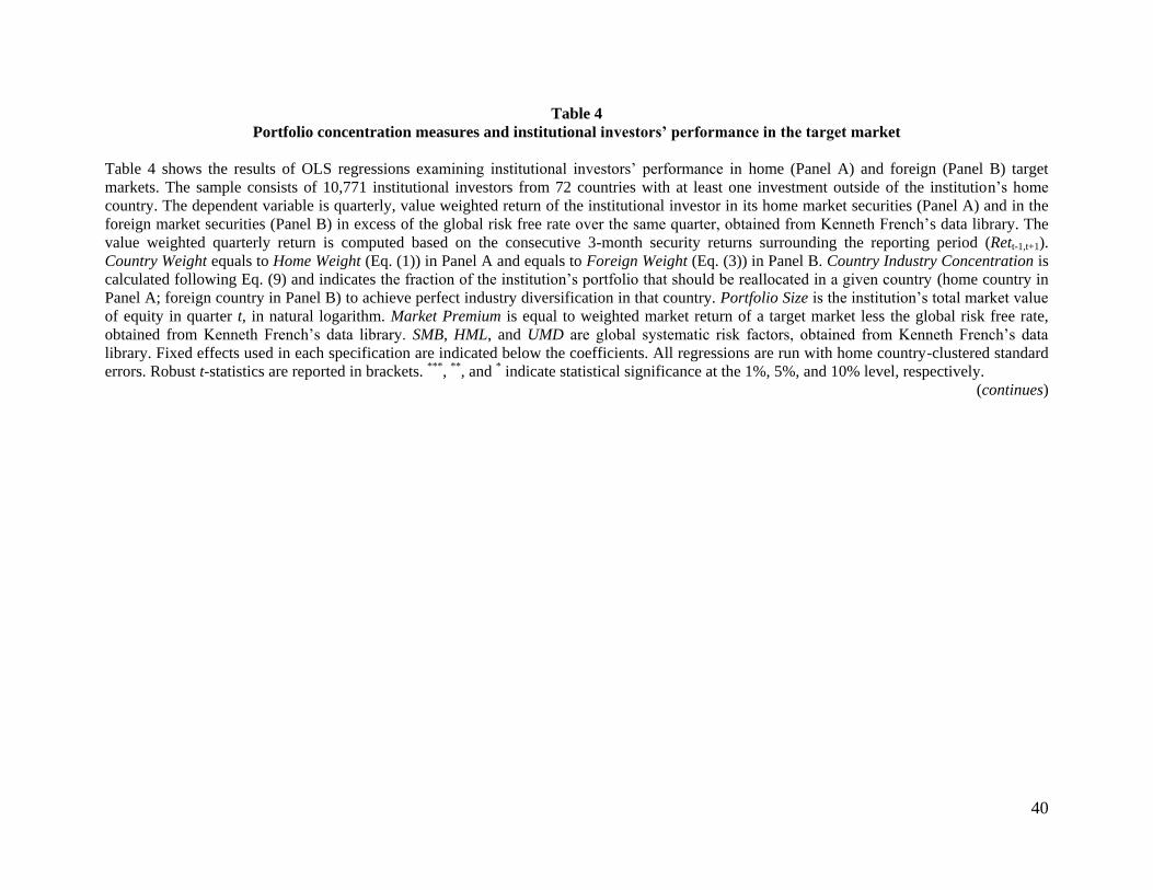
Table 4

Portfolio concentration measures and institutional investors’ performance in the target market

Table 4 shows the results of OLS regressions examining institutional investors’ performance in home (Panel A) and foreign (Panel B) target

markets. The sample consists of 10,771 institutional investors from 72 countries with at least one investment outside of the institution’s home

country. The dependent variable is quarterly, value weighted return of the institutional investor in its home market securities (Panel A) and in the

foreign market securities (Panel B) in excess of the global risk free rate over the same quarter, obtained from Kenneth French’s data library. The

value weighted quarterly return is computed based on the consecutive 3-month security returns surrounding the reporting period (Rett-1,t+1).

Country Weight equals to Home Weight (Eq. (1)) in Panel A and equals to Foreign Weight (Eq. (3)) in Panel B. Country Industry Concentration is

calculated following Eq. (9) and indicates the fraction of the institution’s portfolio that should be reallocated in a given country (home country in

Panel A; foreign country in Panel B) to achieve perfect industry diversification in that country. Portfolio Size is the institution’s total market value

of equity in quarter t, in natural logarithm. Market Premium is equal to weighted market return of a target market less the global risk free rate,

obtained from Kenneth French’s data library. SMB, HML, and UMD are global systematic risk factors, obtained from Kenneth French’s data

library. Fixed effects used in each specification are indicated below the coefficients. All regressions are run with home country-clustered standard

errors. Robust t-statistics are reported in brackets. ***, **, and * indicate statistical significance at the 1%, 5%, and 10% level, respectively.

(continues)

41

Table 4 (continued)

Panel A: Home market performance Panel B: Foreign market performance

(1) (2) (3) (4) (1) (2) (3) (4)

Country Weight 0.0038***

0.0027*** 0.0027***

0.0039***

0.0064*** 0.0077***

[3.75]

[2.80] [2.72]

[2.70]

[4.10] [4.69]

Country Industry Concentration 0.0115*** 0.0104*** 0.0107***

0.0054*** 0.0061*** 0.0066***

[3.59] [2.95] [3.40] [3.26] [3.58] [3.86]

Portfolio Size -0.0005*** -0.0001 -0.0002* -0.0001

-0.0021 -0.0006 0.0007 0.0027*

[-3.44] [-1.29] [-1.78] [-0.37]

[-1.56] [-0.36] [0.41] [1.73]

Market Premium 0.9300*** 0.9302*** 0.9302*** 0.9158***

0.9623*** 0.9519*** 0.9519*** 0.9396***

[14.10] [14.08] [14.09] [11.19]

[64.10] [66.35] [66.34] [61.74]

SMB

-0.2972***

-0.1753***

[-4.84]

[-5.62]

HML

-0.3082***

-0.1760***

[-3.65]

[-7.27]

UMD

-0.1301**

-0.1078***

[-2.38]

[-11.11]

Fixed Effects Home Home Home Home

Home Home Home Home

Target Target Target Target

Year Year Year Year

Year Year Year Year

Style Style Style Style


Type Type Type Type Type Type Type Type

Number of Observations 112,584 112,584 112,584 112,584

1,184,360 1,128,619 1,128,619 1,128,619

Adjusted R2 0.6169 0.6170 0.6171 0.6258 0.5044 0.5110 0.5110 0.5158

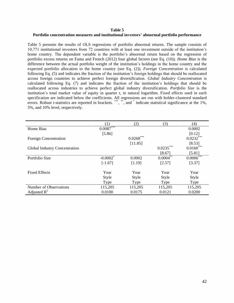
42

Table 5 Portfolio concentration measures and institutional investors’ abnormal portfolio performance

Table 5 presents the results of OLS regressions of portfolio abnormal returns. The sample consists of

10,771 institutional investors from 72 countries with at least one investment outside of the institution’s

home country. The dependent variable is the portfolio’s abnormal return based on the regression of

portfolio excess returns on Fama and French (2012) four global factors (see Eq. (10)). Home Bias is the


expected portfolio allocation to the home country (see Eq. (2)). Foreign Concentration is calculated

following Eq. (5) and indicates the fraction of the institution’s foreign holdings that should be reallocated

across foreign countries to achieve perfect foreign diversification. Global Industry Concentration is

calculated following Eq. (7) and indicates the fraction of the institution’s holdings that should be

reallocated across industries to achieve perfect global industry diversification. Portfolio Size is the

institution’s total market value of equity in quarter t, in natural logarithm. Fixed effects used in each

specification are indicated below the coefficients. All regressions are run with holder-clustered standard

errors. Robust t-statistics are reported in brackets. ***, **, and * indicate statistical significance at the 1%,

5%, and 10% level, respectively.

(1) (2) (3) (4)

Home Bias 0.0087***

0.0002

[5.86]

[0.12]


0.0268***

0.0232***

[11.85]

[8.53]


0.0235*** 0.0160***

[8.67] [5.81]

Portfolio Size -0.0002* 0.0002 0.0004** 0.0006***

[-1.67] [1.19] [2.57] [3.37]

Fixed Effects Year Year Year Year


Type Type Type Type

Number of Observations 115,205 115,205 115,205 115,205

Adjusted R2 0.0100 0.0175 0.0121 0.0200

43

Table 6

Portfolio concentration and performance of mutual and non-mutual funds

Table 6 reports the results of OLS regressions of portfolio concentration measures and performance run

separately for mutual fund and non-mutual fund institutional investors. Institution’s type is indicated as

MF (mutual fund) or non-MF (non-mutual fund). Panel A presents the results for portfolio level

performance. Panels B and C examine the institutions’ performance in the home and foreign target

markets, respectively. Home Bias is the difference between the actual portfolio weight of the institution’s

holdings in the home country and the expected portfolio allocation to the home country (see Eq. (2)).

Foreign Concentration is calculated following Eq. (5) and indicates the fraction of the institution’s

foreign holdings that should be reallocated across foreign countries to achieve perfect foreign

diversification. Global Industry Concentration is calculated following Eq. (7) and indicates the fraction of

the institution’s holdings that should be reallocated across industries to achieve perfect global industry

diversification. Portfolio Size is the institution’s total market value of equity in quarter t, in natural

logarithm. Market Premium is obtained from Kenneth French’s website when evaluating overall portfolio

performance (Panel A) and calculated as equal weighted market return of a target market less global risk

free rate when evaluating the target market performance (Panel B and C). Fixed effects used in each

specification are indicated below the coefficients. Panel A’s regressions are run with holder-clustered

standard errors; Panel B’s regressions are run with home country clustered errors; Panel C’s regressions

are run with two-way (home country – target country) clustered errors. Robust t-statistics are reported in

brackets. ***, **, and * indicate statistical significance at the 1%, 5%, and 10% level, respectively.

(continues)

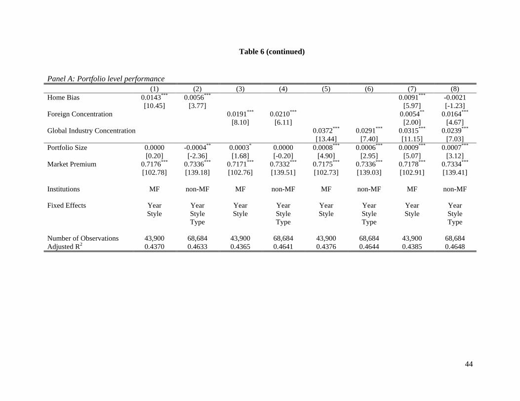
44

Table 6 (continued)

Panel A: Portfolio level performance

(1) (2) (3) (4) (5) (6) (7) (8)

Home Bias 0.0143*** 0.0056***

0.0091*** -0.0021

[10.45] [3.77]

[5.97] [-1.23]


0.0191*** 0.0210***

0.0054** 0.0164***

[8.10] [6.11]

[2.00] [4.67]


0.0372*** 0.0291*** 0.0315*** 0.0239***

[13.44] [7.40] [11.15] [7.03]

Portfolio Size 0.0000 -0.0004** 0.0003* 0.0000 0.0008*** 0.0006*** 0.0009*** 0.0007***

[0.20] [-2.36] [1.68] [-0.20] [4.90] [2.95] [5.07] [3.12]

Market Premium 0.7176*** 0.7336*** 0.7171*** 0.7332*** 0.7175*** 0.7336*** 0.7178*** 0.7334***

[102.78] [139.18] [102.76] [139.51] [102.73] [139.03] [102.91] [139.41]

Institutions MF non-MF MF non-MF MF non-MF MF non-MF

Fixed Effects Year Year Year Year Year Year Year Year

Style Style Style Style Style Style Style Style

Type

Type

Type

Type

Number of Observations 43,900 68,684 43,900 68,684 43,900 68,684 43,900 68,684

Adjusted R2 0.4370 0.4633 0.4365 0.4641 0.4376 0.4644 0.4385 0.4648

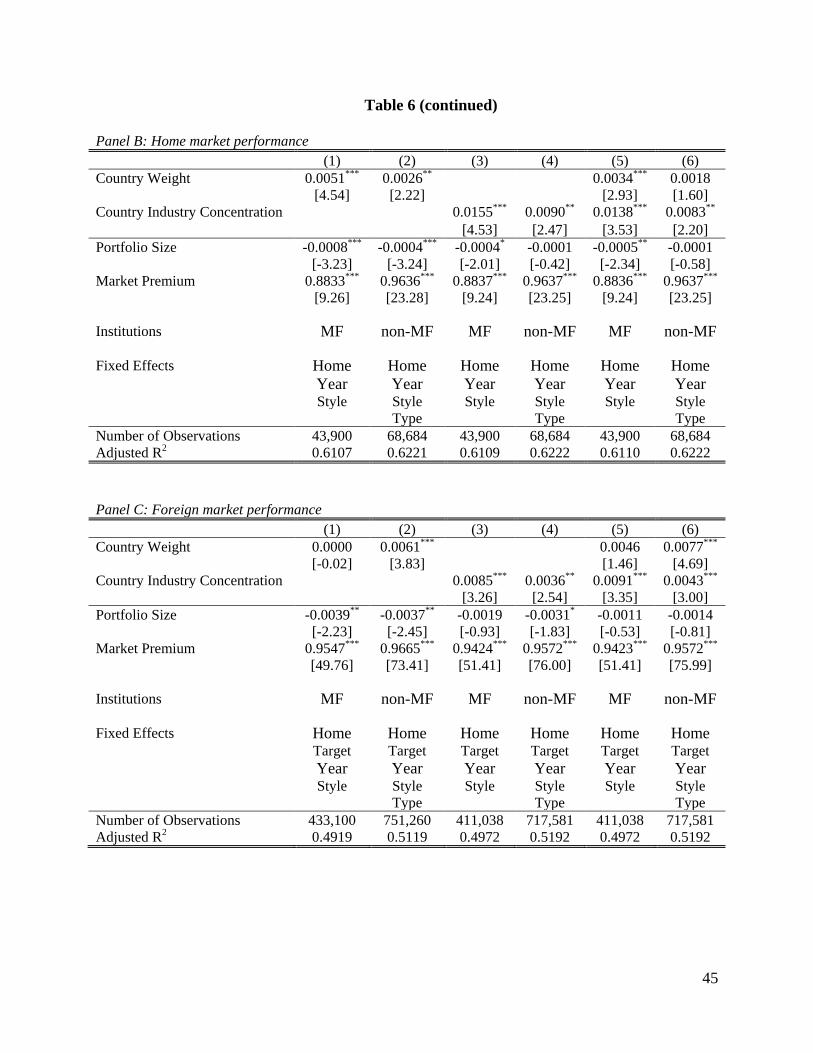
45

Table 6 (continued)

Panel B: Home market performance

(1) (2) (3) (4) (5) (6)

Country Weight 0.0051*** 0.0026**

0.0034*** 0.0018

[4.54] [2.22]

[2.93] [1.60]

Country Industry Concentration

0.0155*** 0.0090** 0.0138*** 0.0083**

[4.53] [2.47] [3.53] [2.20]

Portfolio Size -0.0008*** -0.0004*** -0.0004* -0.0001 -0.0005** -0.0001

[-3.23] [-3.24] [-2.01] [-0.42] [-2.34] [-0.58]

Market Premium 0.8833*** 0.9636*** 0.8837*** 0.9637*** 0.8836*** 0.9637***

[9.26] [23.28] [9.24] [23.25] [9.24] [23.25]

Institutions MF non-MF MF non-MF MF non-MF

Fixed Effects Home Home Home Home Home Home

Year Year Year Year Year Year

Style Style Style Style Style Style

Type

Type

Type

Number of Observations 43,900 68,684 43,900 68,684 43,900 68,684

Adjusted R2 0.6107 0.6221 0.6109 0.6222 0.6110 0.6222

Panel C: Foreign market performance

(1) (2) (3) (4) (5) (6)

Country Weight 0.0000 0.0061***

0.0046 0.0077***

[-0.02] [3.83]

[1.46] [4.69]

Country Industry Concentration

0.0085*** 0.0036** 0.0091*** 0.0043***

[3.26] [2.54] [3.35] [3.00]

Portfolio Size -0.0039** -0.0037** -0.0019 -0.0031* -0.0011 -0.0014

[-2.23] [-2.45] [-0.93] [-1.83] [-0.53] [-0.81]

Market Premium 0.9547*** 0.9665*** 0.9424*** 0.9572*** 0.9423*** 0.9572***

[49.76] [73.41] [51.41] [76.00] [51.41] [75.99]

Institutions MF non-MF MF non-MF MF non-MF

Fixed Effects Home Home Home Home Home Home

Target Target Target Target Target Target

Year Year Year Year Year Year

Style Style Style Style Style Style

Type

Type

Type

Number of Observations 433,100 751,260 411,038 717,581 411,038 717,581

Adjusted R2 0.4919 0.5119 0.4972 0.5192 0.4972 0.5192

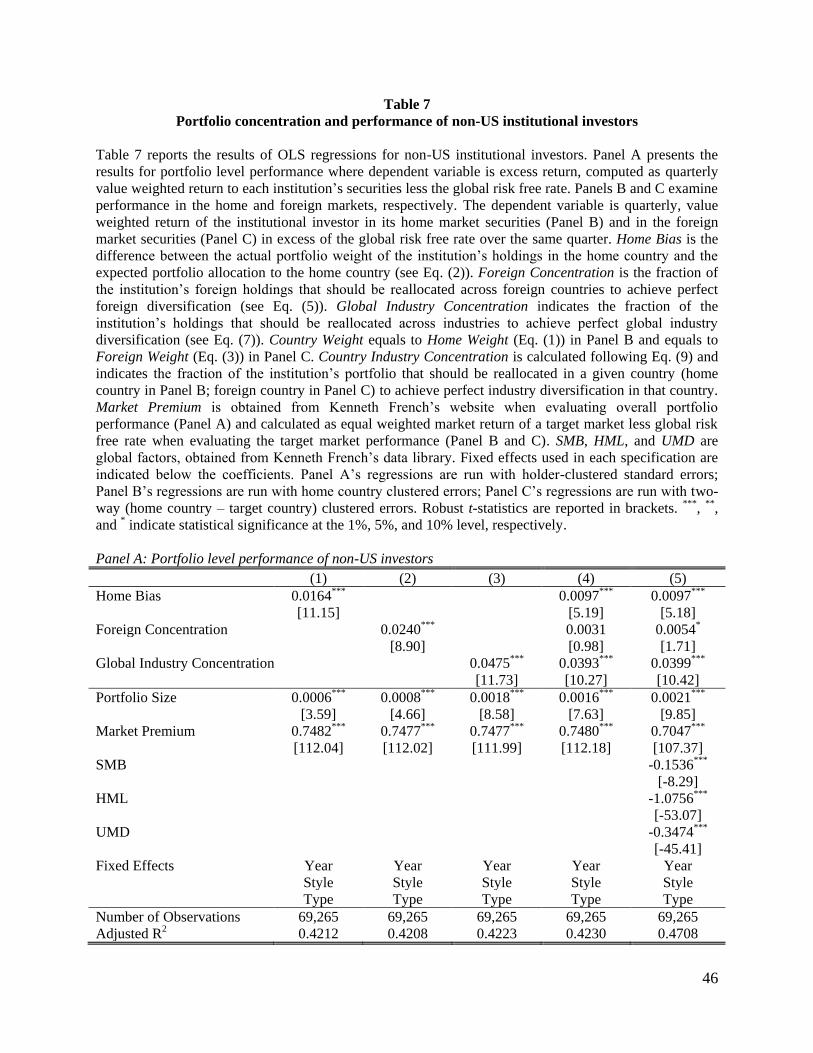
46

Table 7

Portfolio concentration and performance of non-US institutional investors

Table 7 reports the results of OLS regressions for non-US institutional investors. Panel A presents the

results for portfolio level performance where dependent variable is excess return, computed as quarterly

value weighted return to each institution’s securities less the global risk free rate. Panels B and C examine

performance in the home and foreign markets, respectively. The dependent variable is quarterly, value

weighted return of the institutional investor in its home market securities (Panel B) and in the foreign

market securities (Panel C) in excess of the global risk free rate over the same quarter. Home Bias is the


expected portfolio allocation to the home country (see Eq. (2)). Foreign Concentration is the fraction of

the institution’s foreign holdings that should be reallocated across foreign countries to achieve perfect

foreign diversification (see Eq. (5)). Global Industry Concentration indicates the fraction of the

institution’s holdings that should be reallocated across industries to achieve perfect global industry

diversification (see Eq. (7)). Country Weight equals to Home Weight (Eq. (1)) in Panel B and equals to

Foreign Weight (Eq. (3)) in Panel C. Country Industry Concentration is calculated following Eq. (9) and

indicates the fraction of the institution’s portfolio that should be reallocated in a given country (home

country in Panel B; foreign country in Panel C) to achieve perfect industry diversification in that country.

Market Premium is obtained from Kenneth French’s website when evaluating overall portfolio

performance (Panel A) and calculated as equal weighted market return of a target market less global risk

free rate when evaluating the target market performance (Panel B and C). SMB, HML, and UMD are

global factors, obtained from Kenneth French’s data library. Fixed effects used in each specification are

indicated below the coefficients. Panel A’s regressions are run with holder-clustered standard errors;

Panel B’s regressions are run with home country clustered errors; Panel C’s regressions are run with two-

way (home country – target country) clustered errors. Robust t-statistics are reported in brackets. ***, **,

and * indicate statistical significance at the 1%, 5%, and 10% level, respectively.

Panel A: Portfolio level performance of non-US investors

(1) (2) (3) (4) (5)

Home Bias 0.0164***

0.0097*** 0.0097***

[11.15]

[5.19] [5.18]

Foreign Concentration 0.0240***

0.0031 0.0054*

[8.90]

[0.98] [1.71]


0.0475*** 0.0393*** 0.0399***

[11.73] [10.27] [10.42]

Portfolio Size 0.0006*** 0.0008*** 0.0018*** 0.0016*** 0.0021***

[3.59] [4.66] [8.58] [7.63] [9.85]

Market Premium 0.7482*** 0.7477*** 0.7477*** 0.7480*** 0.7047***

[112.04] [112.02] [111.99] [112.18] [107.37]

SMB

-0.1536***

[-8.29]

HML

-1.0756***

[-53.07]

UMD

-0.3474***

[-45.41]

Fixed Effects Year Year Year Year Year

Style Style Style Style Style

Type Type Type Type Type

Number of Observations 69,265 69,265 69,265 69,265 69,265

Adjusted R2 0.4212 0.4208 0.4223 0.4230 0.4708

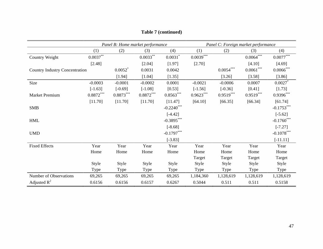
47

Table 7 (continued)

Panel B: Home market performance Panel C: Foreign market performance

(1) (2) (3) (4) (1) (2) (3) (4)

Country Weight 0.0037**

0.0033** 0.0031* 0.0039***

0.0064*** 0.0077***

[2.48]

[2.04] [1.97] [2.70]

[4.10] [4.69]

Country Industry Concentration 0.0052* 0.0031 0.0042

0.0054*** 0.0061*** 0.0066***

[1.94] [1.04] [1.35]

[3.26] [3.58] [3.86]

Size -0.0003 -0.0001 -0.0002 0.0001 -0.0021 -0.0006 0.0007 0.0027*

[-1.63] [-0.69] [-1.08] [0.53] [-1.56] [-0.36] [0.41] [1.73]

Market Premium 0.8872*** 0.8873*** 0.8872*** 0.8563*** 0.9623*** 0.9519*** 0.9519*** 0.9396***

[11.70] [11.70] [11.70] [11.47] [64.10] [66.35] [66.34] [61.74]

SMB

-0.2240***

-0.1753***

[-4.42]

[-5.62]

HML

-0.3895***

-0.1760***

[-8.68]

[-7.27]

UMD

-0.1797***

-0.1078***

[-3.83]

[-11.11]

Fixed Effects Year Year Year Year Year Year Year Year

Home Home Home Home Home Home Home Home

Target Target Target Target

Style Style Style Style Style Style Style Style

Type Type Type Type Type Type Type Type

Number of Observations 69,265 69,265 69,265 69,265 1,184,360 1,128,619 1,128,619 1,128,619

Adjusted R2 0.6156 0.6156 0.6157 0.6267 0.5044 0.511 0.511 0.5158

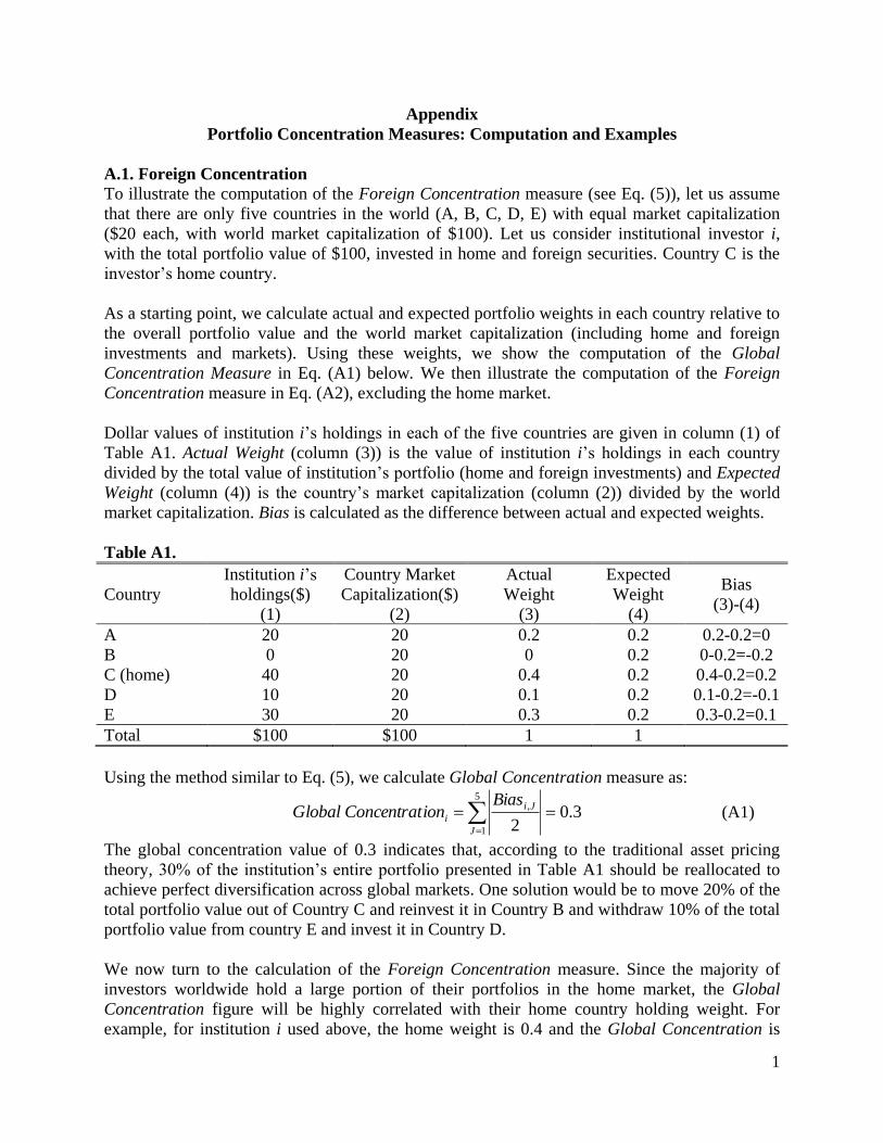
1

Appendix

Portfolio Concentration Measures: Computation and Examples

A.1. Foreign Concentration

To illustrate the computation of the Foreign Concentration measure (see Eq. (5)), let us assume

that there are only five countries in the world (A, B, C, D, E) with equal market capitalization

($20 each, with world market capitalization of $100). Let us consider institutional investor i,

with the total portfolio value of $100, invested in home and foreign securities. Country C is the

investor’s home country.

As a starting point, we calculate actual and expected portfolio weights in each country relative to

the overall portfolio value and the world market capitalization (including home and foreign

investments and markets). Using these weights, we show the computation of the Global

Concentration Measure in Eq. (A1) below. We then illustrate the computation of the Foreign

Concentration measure in Eq. (A2), excluding the home market.

Dollar values of institution i’s holdings in each of the five countries are given in column (1) of

Table A1. Actual Weight (column (3)) is the value of institution i’s holdings in each country

divided by the total value of institution’s portfolio (home and foreign investments) and Expected

Weight (column (4)) is the country’s market capitalization (column (2)) divided by the world

market capitalization. Bias is calculated as the difference between actual and expected weights.

Table A1.

Country

Institution i’s

holdings($)

(1)

Country Market

Capitalization($)

(2)

Actual

Weight

(3)

Expected

Weight

(4)

Bias

(3)-(4)

A 20 20 0.2 0.2 0.2-0.2=0

B 0 20 0 0.2 0-0.2=-0.2

C (home) 40 20 0.4 0.2 0.4-0.2=0.2

D 10 20 0.1 0.2 0.1-0.2=-0.1

E 30 20 0.3 0.2 0.3-0.2=0.1

Total $100 $100 1 1

Using the method similar to Eq. (5), we calculate Global Concentration measure as:

3.02

5

1

,

J

Ji

i

BiasionConcentratGlobal (A1)

The global concentration value of 0.3 indicates that, according to the traditional asset pricing

theory, 30% of the institution’s entire portfolio presented in Table A1 should be reallocated to

achieve perfect diversification across global markets. One solution would be to move 20% of the

total portfolio value out of Country C and reinvest it in Country B and withdraw 10% of the total

portfolio value from country E and invest it in Country D.

We now turn to the calculation of the Foreign Concentration measure. Since the majority of

investors worldwide hold a large portion of their portfolios in the home market, the Global

Concentration figure will be highly correlated with their home country holding weight. For

example, for institution i used above, the home weight is 0.4 and the Global Concentration is

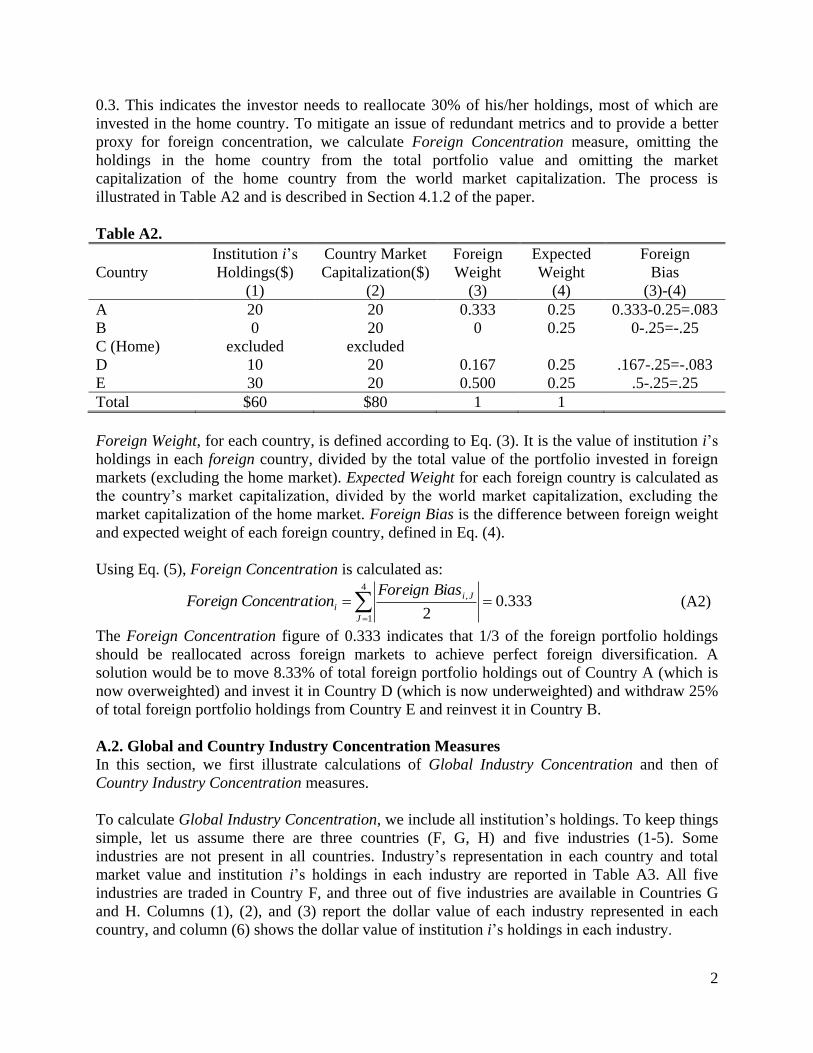
2

0.3. This indicates the investor needs to reallocate 30% of his/her holdings, most of which are

invested in the home country. To mitigate an issue of redundant metrics and to provide a better

proxy for foreign concentration, we calculate Foreign Concentration measure, omitting the

holdings in the home country from the total portfolio value and omitting the market

capitalization of the home country from the world market capitalization. The process is

illustrated in Table A2 and is described in Section 4.1.2 of the paper.

Table A2.

Country

Institution i’s

Holdings($)

(1)

Country Market

Capitalization($)

(2)

Foreign

Weight

(3)

Expected

Weight

(4)

Foreign

Bias

(3)-(4)

A 20 20 0.333 0.25 0.333-0.25=.083

B 0 20 0 0.25 0-.25=-.25

C (Home) excluded excluded

D 10 20 0.167 0.25 .167-.25=-.083

E 30 20 0.500 0.25 .5-.25=.25

Total $60 $80 1 1

Foreign Weight, for each country, is defined according to Eq. (3). It is the value of institution i’s

holdings in each foreign country, divided by the total value of the portfolio invested in foreign

markets (excluding the home market). Expected Weight for each foreign country is calculated as

the country’s market capitalization, divided by the world market capitalization, excluding the

market capitalization of the home market. Foreign Bias is the difference between foreign weight

and expected weight of each foreign country, defined in Eq. (4).

Using Eq. (5), Foreign Concentration is calculated as:

333.02

4

1

, J

Ji

i

BiasForeignionConcentratForeign (A2)

The Foreign Concentration figure of 0.333 indicates that 1/3 of the foreign portfolio holdings

should be reallocated across foreign markets to achieve perfect foreign diversification. A

solution would be to move 8.33% of total foreign portfolio holdings out of Country A (which is

now overweighted) and invest it in Country D (which is now underweighted) and withdraw 25%

of total foreign portfolio holdings from Country E and reinvest it in Country B.

A.2. Global and Country Industry Concentration Measures

In this section, we first illustrate calculations of Global Industry Concentration and then of

Country Industry Concentration measures.

To calculate Global Industry Concentration, we include all institution’s holdings. To keep things

simple, let us assume there are three countries (F, G, H) and five industries (1-5). Some

industries are not present in all countries. Industry’s representation in each country and total

market value and institution i’s holdings in each industry are reported in Table A3. All five

industries are traded in Country F, and three out of five industries are available in Countries G

and H. Columns (1), (2), and (3) report the dollar value of each industry represented in each

country, and column (6) shows the dollar value of institution i’s holdings in each industry.

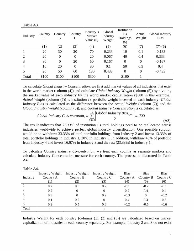
3

Table A3.

Industry Country

F

Country

G

Country

H

Industry’s

Market

Value ($)

Global

Industry

Weight

Institution

i’s

Holdings

($)

Actual

Weight

Global Industry

Bias

(1) (2) (3) (4) (5) (6) (7) (7)-(5)

1 20 30 20 70 0.233 10 0.1 -0.133

2 20 0 0 20 0.067 40 0.4 0.333

3 30 0 20 50 0.167 0 0 -0.167

4 10 20 0 30 0.1 50 0.5 0.4

5 20 50 60 130 0.433 0 0 -0.433

Total $100 $100 $100 $300 1 $100 1

To calculate Global Industry Concentration, we first add market values of all industries that exist

in the world market (column (4)) and calculate Global Industry Weight (column (5)) by dividing

the market value of each industry by the world market capitalization ($300 in this example).

Actual Weight (column (7)) is institution i's portfolio weight invested in each industry. Global

Industry Bias is calculated as the difference between the Actual Weight (column (7)) and the

Global Industry Weight (column (5)), and Global Industry Concentration is calculated as:

733.2

5

1

, SIC

SICi

i

BiasIndustryGlobalionConcentratIndustryGlobal

(A3)

The result indicates that 73.33% of institution i’s total holdings need to be reallocated across

industries worldwide to achieve perfect global industry diversification. One possible solution

would be to withdraw 33.33% of total portfolio holdings from Industry 2 and invest 13.33% of

total portfolio holdings in Industry 1, 20% in Industry 5. In addition, withdraw 40% of portfolio

from Industry 4 and invest 16.67% in Industry 3 and the rest (23.33%) in Industry 5.

To calculate Country Industry Concentration, we treat each country as separate markets and

calculate Industry Concentration measure for each country. The process is illustrated in Table

A4.

Table A4.

Industry

Industry Weight

Country A

(1)

Industry Weight

Country B

(2)

Industry Weight

Country C

(3)

Bias

Country A

(4)

Bias

Country B

(5)

Bias

Country C

(6)

1 0.2 0.3 0.2 -0.1 -0.2 -0.1

2 0.2 0 0 0.2 0.4 0.4

3 0.3 0 0.2 -0.3 0 -0.2

4 0.1 0.2 0 0.4 0.3 0.5

5 0.2 0.5 0.6 -0.2 -0.5 -0.6

Total 1 1 1

Industry Weight for each country (columns (1), (2) and (3)) are calculated based on market

capitalization of industries in each country separately. For example, Industry 2 and 3 do not exist

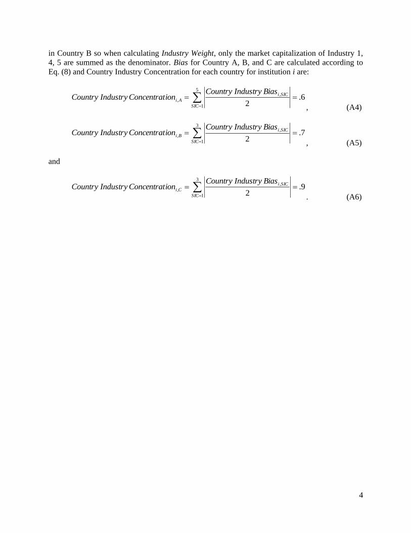
4

in Country B so when calculating Industry Weight, only the market capitalization of Industry 1,

4, 5 are summed as the denominator. Bias for Country A, B, and C are calculated according to

Eq. (8) and Country Industry Concentration for each country for institution i are:

6.2

5

1

,

, SIC

SICi

Ai

BiasIndustryCountryionConcentratIndustryCountry

, (A4)

7.2

3

1

,

, SIC

SICi

Bi


, (A5)

and

9.2

3

1

,

, SIC

SICi

Ci


. (A6)

Documents

Portfolio Concentration and Performance of … Concentration and Performance of Institutional Investors Worldwide Nicole Choi University of Wyoming 1000 E. University Ave. Laramie,