Embed Size (px)
Citation preview

11
OR 2006Karlsruhe, Germany, September 6-8, 2006
Portfolio Optimization: A Technical Perspective
Franz Neliß[email protected]
GAMS Software GmbHwww.gams.de

22
Agenda
Introduction
Mathematical Optimization in Finance
An illustrative Example: The MeanVariance Model
Advanced Portfolio Optimization Models
Grid Computing

33
Agenda
Introduction
Mathematical Optimization in Finance
An illustrative Example: The MeanVariance Model
Advanced Portfolio Optimization Models
Grid Computing

44
GAMS Development / GAMS Software
• Roots: Research project World Bank 1976
• Pioneer in Algebraic Modeling Systemsused for economic modeling
• Went commercial in 1987• Offices in Washington, D.C
and Cologne
• Professional software tool provider, not a consulting company
• Operating in a segmented niche market
• Broad academic & commercial user baseand network
General Algebraic Modeling System

55
Agenda
Introduction
Mathematical Optimization in Finance
An illustrative Example: The MeanVariance Model
Advanced Portfolio Optimization Models
Grid Computing
66
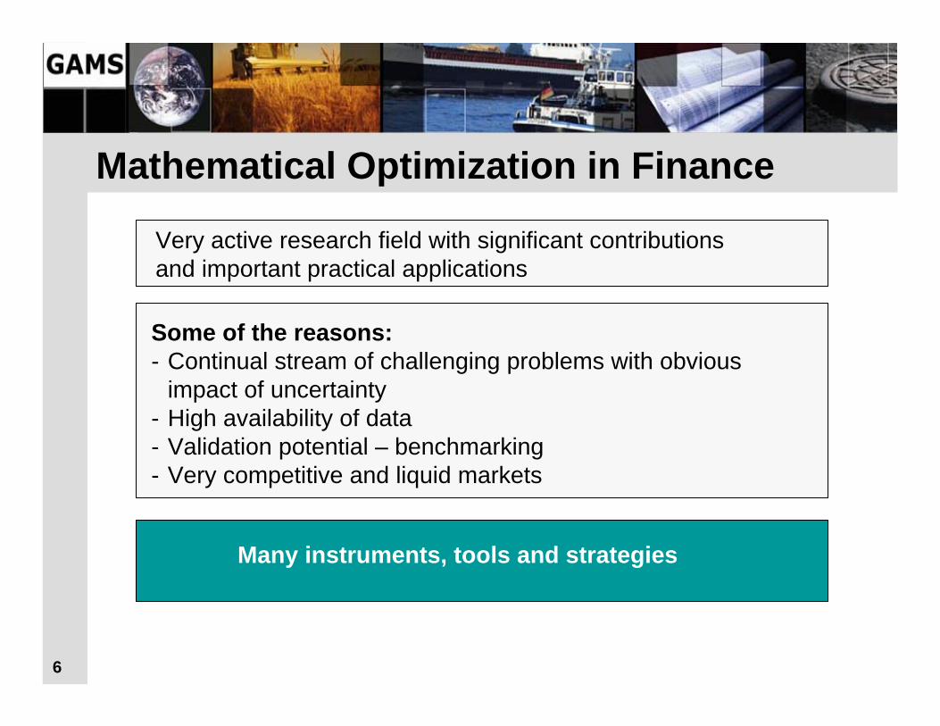
Mathematical Optimization in Finance
Very active research field with significant contributions and important practical applications
Some of the reasons:- Continual stream of challenging problems with obvious
impact of uncertainty - High availability of data- Validation potential – benchmarking- Very competitive and liquid markets
Many instruments, tools and strategies

77
Portfolio Optimization Models
- Mean-Variance Model
- Portfolio models for fixed income
- Scenario optimization
- Stochastic programming

88
Change in Focus
ComputationPast
Algorithm limits applicationProblem representation low priorityLarge expensive projects Long development timesCentralized expert groupsHigh computational costsUsers left out
ModelNow
Modeling skill limits applicationsAlgebraic model representationSmaller projects and rapid developmentDecentralized modeling teamsMachine independence
Users involved
ApplicationFuture
Domain expertise limits application Off-the-shelf GUIModels embedded in business applicationsLinks to other types of modelsInternet/Web
Users hardly aware of model

99
Modeling Approaches
- Algebraic Modeling Languages - Balanced mix of declarative and procedural elements- Open architecture and interfaces to other systems- Different layers with separation of:
- model and data- model and solution methods- model and operating system- model and interface
- Programming languages: C++, Delphi, Java, VBA, …- Spreadsheets- Specialized tools

1010
AgendaIntroduction
Introduction
Mathematical Optimization in Finance
An illustrative Example: The MeanVariance Model
Advanced Portfolio Optimization Models
Grid Computing

1111
MV Model Algebra
Varianceof Portfolio ∑∑
= =
I
ij
J
jjii xQxMin
1 1,
Targetreturn ∑
=
≥I
iii rxts
1.. µ
Budgetconstraint ∑
=
=I
iix
11
No shortsales
0≥ix

1212
Declarative Model and some Data

1313
Modeling Issues
Basic MV-Model: Quadratic model
Solver- NLP Codes (CONOPT, MINOS,...) or- QCP Codes (Cplex, Mosek, Xpress)
- take advantage of special structure
Large problem instances can be solved routinely

1414
Business Rules
- Institutional or legal requirements- Additional constraints, which have to be satisfied- Trading restrictions- Not defined by modeling experts- Independent of risk model
Simple business rules: Do not change the model type:- Short selling- Risk free borrowing- Upper or lower bounds on certain instruments

1515
More Complex Business Rules
Require introduction of integer (binary) variables:
– Cardinality Constraint: Restrict number of investments yi in portfolio
– Threshold Constraint: Investments xi can only be purchased at certain minimum ll,i or maximum lu,I
– more trading restrictions …
1616
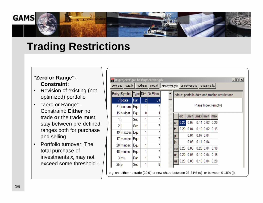
"Zero or Range"-Constraint:
• Revision of existing (not optimized) portfolio
• "Zero or Range“ -Constraint: Either no trade or the trade must stay between pre-defined ranges both for purchase and selling
• Portfolio turnover: The total purchase of investments xi may not exceed some threshold τ
Trading Restrictions
e.g. cn: either no trade (20%) or new share between 23-31% (u) or between 0-18% (l)

1717
GAMS FormulationVariablesxi(i) fraction of portfolio increase,xd(i) fraction of portfolio decrease,y(i) binary switch for increasing current holdings of i,z(i) binary switch for decreasing current holdings of i;Binary Variables y, z; Positive Variables xi, xd;Equations xdef(i) final portfolio definition,maxinc(i) bound of maximum lot increase of fraction of i,mininc(i) bound of minimum lot increase of fraction of i,maxdec(i) bound of maximum lot decrease of fraction of i,mindec(i) bound of minimum lot decrease of fraction of i,binsum(i) restricts use of binary variables,turnover restricts maximum turnover of portfolio;
xdef(i).. x(i) =e= bdata(i,'old') -xd(i) + xi(i);maxinc(i).. xi(i) =l= bdata(i,'umax')* y(i);mininc(i).. xi(i) =g= bdata(i,'umin')* y(i);maxdec(i).. xd(i) =l= bdata(i,'lmax')* z(i);mindec(i).. xd(i) =g= bdata(i,'lmin')* z(i);binsum(i).. y(i) + z(i) =l= 1;turnover.. sum(i, xi(i)) =l= tau;
Model Type:MIQCP

1818
Procedural Elements$gdxin data # get data & setup model$load i mu q q(i,j) = 2*q(j,i) ; q(i,i) = q(i,i)/2;Model var / all / ; set p points for efficient frontier /minv, p1*p8, maxr/,
pp(p) points used for loop / p1*p8 /;parameter minr, maxr,rep(p,*), repx(p,i);
# get bounds for efficient frontiersolve var minimizing v using miqcp; #find portfolio with minimal varianceminr = r.l; rep('minv','ret') = r.l; rep('minv','var') = v.l; repx('minv',i) = x.l(i);
solve var maximizing r using miqcp; #find portfolio with maximal returnmaxr = r.l; rep('maxr','ret')= r.l;rep('maxr','var')=v.l;repx('maxr',i)= x.l(i);
loop(pp, #calculate efficient frontierr.fx = minr + (maxr-minr)/(card(pp)+1)*ord(pp);solve var minimizing v using miqcp;rep(pp,'ret') =r.l;rep(pp,'var') = v.l;repx(pp,i)= x.l(i);
);
Execute_Unload 'results.gdx',rep, repx; # export results to GDX & ExcelExecute 'GDXXRW.EXE results.gdx par=repx rng=Portfolio!a1 Rdim=1';Execute 'GDXXRW.EXE results.gdx par=rep rng=Frontier!a1 Rdim=1';

1919
Share of portfolio (%)
Solution points
CanadaFranceGreeceJapan
SwedenUKUS
oldr minvar
p1 p2 maxret
p3 p10p4 p9p8p5 p7p60
0.02
0.04
0.06
0.08
0.1
0.12
0.14
0.16
0 5 10 15 20 25 30
Return of portfolio (%)
Variance of portfolio
Efficient Frontier and Portfolios (τ = 0.3)

2020
Scenario Optimization ModelsScenarios capture complex interactions between multiple risk
factors• Different methods for risk measurement:
– Mean Absolute Deviation Models– Index Tracking Models– Expected Utility Models– VAR Models (linear Version: CVAR)
• Models are solved over all scenarios
Modeling Issues:• Linear Models, but business rules may introduce binary
variables• Lots of independent scenarios, which can be handled in
parallel
2121
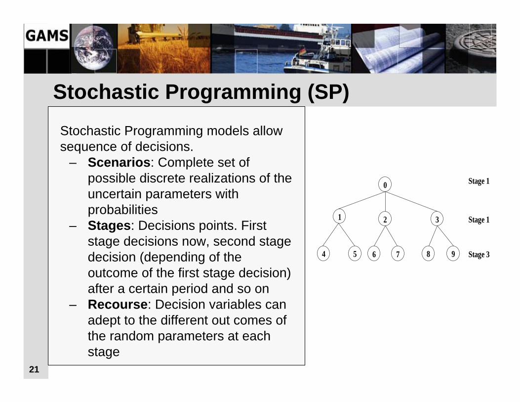
Stochastic Programming (SP)Stochastic Programming models allow sequence of decisions.
– Scenarios: Complete set of possible discrete realizations of the uncertain parameters with probabilities
– Stages: Decisions points. First stage decisions now, second stage decision (depending of the outcome of the first stage decision) after a certain period and so on
– Recourse: Decision variables can adept to the different out comes of the random parameters at each stage
0
4
31 2
6 85
Stage 1
Stage 1
Stage 397

2222
More Complex Scenario Trees
2323
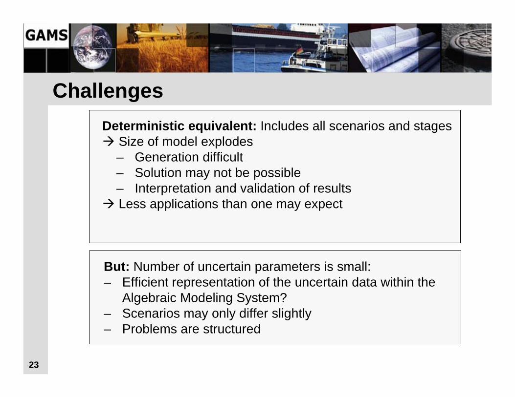
ChallengesDeterministic equivalent: Includes all scenarios and stages
Size of model explodes– Generation difficult– Solution may not be possible– Interpretation and validation of resultsLess applications than one may expect
But: Number of uncertain parameters is small:– Efficient representation of the uncertain data within the
Algebraic Modeling System?– Scenarios may only differ slightly – Problems are structured

2424
Current DevelopmentsNew language elements :- Special expressions and conventions for stages and
scenario trees- Random distributions for some problem data- Support of scenario reduction techniques dramatically
reduces the size of deterministic equivalent- Automatic translation of problem description into format
for various SP-solvers (DECIS, SPLINE…)- Support for parallel optimization
But: - Different approaches- Not yet clear which standards will be adopted

2525
More Theory and Templates
Theory
• Practical Financial Optimization (forthcoming) by S. Zenios
• A Library of Financial Optimization Models (forthcoming) by A. Consiglio, S. Nielsen, H. Vladimirou and S. Zenios
• Financial Optimization by S. Zenios (ed.)
Templatesavailableonline
• GAMS Model Library: http://www.gams.com/modlib/libhtml/subindx.htm
• Course Notes „Financial Optimization“:http://www.gams.com/docs/contributed/financial/

2626
AgendaIntroduction
Introduction
Mathematical Optimization in Finance
An illustrative Example: The MeanVariance Model
Advanced Portfolio Optimization Models
Grid Computing

2727
Grid Computing
Imagine….. you have to solve 1.000’s of independent scenarios.... and you can do this very rapidly for little additional money….. without having to do lots of cumbersome programming work..
loop(pp, #calculate efficient frontierr.fx = minr + (maxr-minr)/(card(pp)+1)*ord(pp);solve var minimizing v using miqcp;rep(pp,'ret') =r.l;rep(pp,'var') = v.l;repx(pp,i)= x.l(i); );
Grid Computing

2828
What is Grid Computing?
A pool of connected computers managed andavailable as a common computing resource
• Effective sharing of CPU power
• Massive parallel task execution
• Scheduler handles management tasks
• E.g. Condor, Sun Grid Engine, Globus
• Can be rented or owned in common
• Licensing & security issues

2929
Advantages of Grid Computing
* http://www.tc.cornell.edu/NR/shared/Presentations/24Feb04.Garp.pdf
• Solve a certain number of scenarios faster, e.g:– sequential: 50 hours– parallel (200 CPUs): ~15 minutes
Cost is $100 (2$ CPU/h)• Get better results by running more scenarios*:
3030
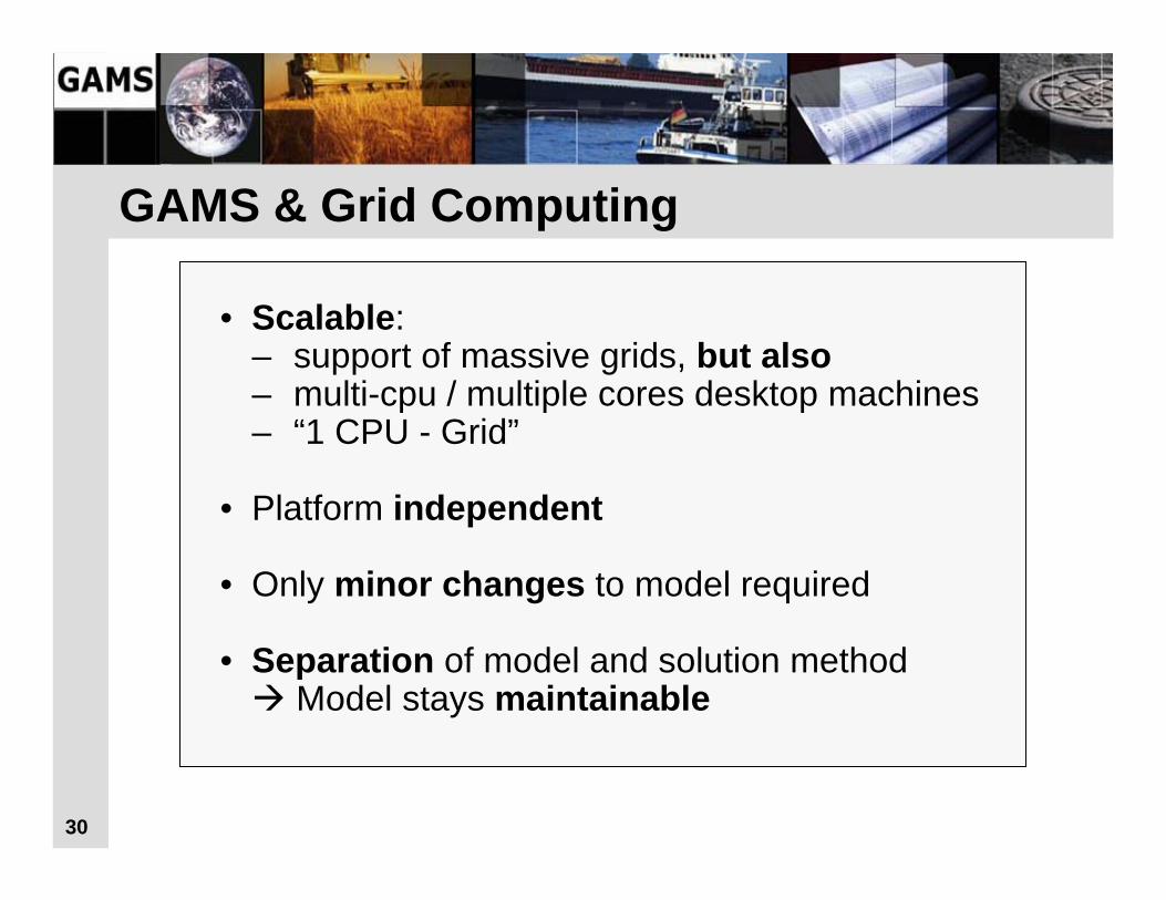
GAMS & Grid Computing
• Scalable:– support of massive grids, but also– multi-cpu / multiple cores desktop machines– “1 CPU - Grid”
• Platform independent
• Only minor changes to model required
• Separation of model and solution methodModel stays maintainable

3131
Simple Serial Solve Loop
Loop(p(pp),
ret.fx = rmin +(rmax-rmin)/(card(pp)+1)*ord(pp) ;
Solve minvar min var using miqcp;
xres(i,p) = x.l(i);
report(p,i,'inc') = xi.l(i);
report(p,i,'dec') = xd.l(i)
);
Generation
Solution
Update
Loop
How do we get to parallel and distributed computing?

3232
GRID Specific Enhancements
1. Submission of jobs
2. “Grid Middleware”– Distribution of jobs – Job execution
3. Collection of solutions
4. Processing of results

3333
Results for 4096 MIPS on Condor Grid• Submission started Jan 11,16:00• All jobs submitted by Jan 11, 23:00• All jobs returned by Jan 12, 12:40
– 20 hours wall time, 5000 CPU hours– Peak number of CPU’s: 500
Talk: Thursday, 08:30
“Chemie-Hörsaal 1”

3434
Conclusions and Summary• Finance is a success story for OR applications• Rich set of different risk models available
• Incorporating business rules may increase complexity of problems but is essential
• Large classes of problems can be solved without major problems
• Stochastic programming still challenging• Grid Computing now offers lots of promising developments

3535
The End
Thank you!… Questions?

3636
Contacting GAMS
USA:GAMS Development Corp. 1217 Potomac Street, NW Washington, DC 20007USA Phone: +1 202 342 0180 Fax: +1 202 342 0181http://www.gams.com
Europe:GAMS Software GmbHEupener Str. 135-13750933 CologneGermanyPhone: +49 221 949 9170Fax: +49 221 949 9171http://www.gams.de