Portfolio Theories

Philippe J.S. De Brouwer∗

September 1, 2010

Abstract

A brief introduction to the contemporary literature about portfoliotheories.

Contents

1 Introduction 3

2 Chronological Overview 32.1 Homo Rationalis: XVII - XIXth Century . . . . . . . . . . . . 4

2.1.1 Expected Value . . . . . . . . . . . . . . . . . . . . . . 42.1.2 The Law of Large Numbers . . . . . . . . . . . . . . . 52.1.3 St Petersburg Paradox . . . . . . . . . . . . . . . . . . 52.1.4 Expected Utility Theory (EUT) . . . . . . . . . . . . 52.1.5 Cramer’s Solution . . . . . . . . . . . . . . . . . . . . 6

2.2 Behavioural Evidence and Thinking: 1750 till 1950 . . . . . . 72.2.1 Adam Smith (1759) . . . . . . . . . . . . . . . . . . . 72.2.2 Early mentioning of irrational behaviour: Mackay (1841)

and others . . . . . . . . . . . . . . . . . . . . . . . . . 82.2.3 The Ellsberg Paradox described by John F.M. Keynes

in 1921 . . . . . . . . . . . . . . . . . . . . . . . . . . 92.2.4 John F.M. Keynes and Chaos theory (1936) . . . . . . 102.2.5 Maslow’s theory of Hierarchy of Needs (1943) and the

framing heuristic . . . . . . . . . . . . . . . . . . . . . 192.2.6 The Axioms of Von Neuman and Morgenstern . . . . 252.2.7 The Friedman-Savage Puzzle (1948) . . . . . . . . . . 27

2.3 Rational Portfolio Theories (1950s and 1960s) . . . . . . . . . 292.3.1 Modern Portfolio Theory (1952) . . . . . . . . . . . . 29

∗Philippe J.S. De Brouwer is Executive Director at Eperon Asset Management Ltd.(fully owned subsidiary of KBC Group N.V. – The views expressed by the author arestrictly his, and do not necessarily represent those of KBC Group N.V nor any of itssubsidiaries. – email: philippe@de-brouwer.net

1

2.3.2 Markowitz’ Customary Wealth Theory (1952) . . . . . 342.3.3 Roy’s Safety First Portfolio Theory (1952) . . . . . . . 382.3.4 The Allais Paradox (1953) . . . . . . . . . . . . . . . . 402.3.5 Subjective Expected Utility Theory (SEU) (1954) . . 412.3.6 cognitive dissonance (1956) . . . . . . . . . . . . . . . 422.3.7 The Ellsberg Paradox popularized by Daniel Ellsberg

(1961) . . . . . . . . . . . . . . . . . . . . . . . . . . . 422.3.8 The Capital Asset Pricing Model (CAPM – 1961) . . 422.3.9 The Fallacy of Large Numbers (1963) . . . . . . . . . 492.3.10 The Efficient Market Hypothesis (EMH) (1964) . . . . 492.3.11 Models for Lifetime Portfolio Selection - 1968 and 1969 512.3.12 An Intertemporal Capital Asset Pricing Model - 1973 53

2.4 Upcoming challengers from Psychology: the 1970s and theearly 1980s . . . . . . . . . . . . . . . . . . . . . . . . . . . . 532.4.1 Availability Heuristic (1973) . . . . . . . . . . . . . . . 532.4.2 More Heuristics (1974) . . . . . . . . . . . . . . . . . . 542.4.3 Support for CAPM and related theories – 1976 . . . . 542.4.4 Prospect Theory (1979) . . . . . . . . . . . . . . . . . 552.4.5 Framing (1981) . . . . . . . . . . . . . . . . . . . . . . 552.4.6 The Volatility Puzzle (1981) . . . . . . . . . . . . . . . 562.4.7 Judgemental Biases Described (1982) . . . . . . . . . 56

2.5 First Signs of Acceptance for Behavioural Finance: 1985 . . . 572.5.1 The first real evidence of market non-efficiencies . . . 572.5.2 Mental Accounting . . . . . . . . . . . . . . . . . . . . 572.5.3 The Equity Premium Puzzle . . . . . . . . . . . . . . 57

2.6 Towards Acceptance of Behavioural Finance Among Scholars(1985 - 2000) . . . . . . . . . . . . . . . . . . . . . . . . . . . 582.6.1 The late 1980s . . . . . . . . . . . . . . . . . . . . . . 582.6.2 Evidence of Analyst overreaction . . . . . . . . . . . . 612.6.3 The Discussion about the Efficiency of the Stock Mar-

kets . . . . . . . . . . . . . . . . . . . . . . . . . . . . 612.6.4 Loss Aversion and endowment effect . . . . . . . . . . 622.6.5 And more Contributions to the Behavioural Paradigm 622.6.6 Cumulative Prospect Theory (1992) . . . . . . . . . . 622.6.7 A Solution for the Equity Premium Puzzle (1995) . . 632.6.8 Vivid Interest in Utility Optmizing Strategies – 1995-

1997 . . . . . . . . . . . . . . . . . . . . . . . . . . . . 652.6.9 More Evidence . . . . . . . . . . . . . . . . . . . . . . 662.6.10 Critics to Behavioural finance (1998) . . . . . . . . . . 672.6.11 An avalanche of evidence, theorems and books (1998

- 2000) . . . . . . . . . . . . . . . . . . . . . . . . . . . 672.6.12 Behavioural Portfolio Theory (BPT – 2000) . . . . . . 692.6.13 Fallacy of Large Numbers Revisited (2001) . . . . . . 71

2.7 2002: an Excellent Behavioural Finance Year . . . . . . . . . 72

2

2.7.1 Nobel Price in 2002 for Behavioural Finance . . . . . 722.7.2 More Heuristics . . . . . . . . . . . . . . . . . . . . . . 722.7.3 And More Evidence . . . . . . . . . . . . . . . . . . . 73

2.8 Efforts to Bring the Major Paradigms Closer to Each Other . 73

3 An Interpretation of the Milestones 73

Endnotes 75

References 75

1 Introduction

It is worth to build foundations solidly before starting any further construc-tion. In this chapter we illustrate the scientific thinking that paved the roadto Maslowian Portfolio Theory (MaPT) and Target Oriented InvestmentAdvice (TOIA).

We try to find the original ideas and original authors of the different the-ses in order to illustrate the logic in the scientific development and thinkingabout portfolio theories. Therefore we emphasize not only new theories, butalso the paradoxes or puzzles that were a direct incentive to produce thisnew theory.

2 Chronological Overview

During the last century two paradigms competed for general acceptance:

“The Rational Paradigm” here investors are rational and optimize theirutility function (which is smooth, concave and based on final wealth)in order to make decisions, markets are efficient, and each investorneeds one optimal portfolio;

“The Behavioural Paradigm” here investors’ behaviour displays impor-tant biases compared to the rational behaviour (for example, peopleare loss averse, overconfident, and think in “frames”), utility is rela-tive to a reference point and can display concave and convex areas, andtherefore investors do not have one efficient portfolio but have frag-mented portfolios, markets are not efficient (and display for exampletrends and mean reverting patterns).

This struggle between the two paradigms was most pronounced in theXXth century. Success shifted between the paradigms during that centurymultiple times, and the most prominent economists and psychologists wereinvolved. Now it seems widely accepted that investors do display importantdeviations from rational behaviour. It is also a fact that patterns with an

3

information content bigger than zero have been detected, and even out ofsample studies show on past data (with hindsight) the possibility to outper-form some markets.

It is however not so straightforward do claim that this also means the endof the EMH. Even the availability of studies (such example see (Caginalpand Laurent 1998)) where on past data statistically significant profitablestrategies can be found, (to the author’s best knowledge) we lack successfulapplications of such theory. Even if a mechanism worked for the last decades,there is no guarantee that it will to continue for the next decade.1

In order to give insight in the evolution of the thinking about investmentportfolio selection, we present the developments chronological. One excep-tion is the very short introduction to chaos theory, as it is rather independentfrom the rest of this work2 (it is all grouped in one chapter).

2.1 Homo Rationalis: XVII - XIXth Century

2.1.1 Expected Value

Blaise Pascal (June 19, 1623 – August 19, 1662) was challenged by a friend,Antoine Gombaud (self acclaimed “Chevalier de Mere” and writer), with agambling puzzle. The brain teaser was that two players who want to finisha game early and, given the current circumstances of it, want to divide thestakes fairly, based on the chance each has of winning the game from thatpoint. How should they find this “fair amount”?In 1654, he corresponded with Louis de Fermat on the subject of gambling.And it is in the discussion about this problem, that the foundations of themathematical theory of probabilities are laid. From this discussion, thenotion of expected value was introduced.

de Fermat and Pascal are generally considered as the founders of the“theory of probability”, and their work laid the foundations for Leibniz’sformulation of the infinitesimal calculus.3

Pascal used later (in the posthumous published “Pensees”) a probabilis-tic argument, Pascal’s Wager, to justify belief in God and a virtuous life.4

1Mathematically chaotic time series might display patterns for a while, but they canchange as time flow. More insight in this phenomenon is given in Chapter 2.2.4 on page 10

2This is done, because this brief introduction to chaos theory provides important insightin the nature and the behaviour of financial markets. This insight is has many applicationsin financial theories and behavioural finance as developed later in this work.

3Actually, de Fermat was the first person known to have evaluated the integral ofgeneral power functions. Using an ingenious trick, he was able to reduce this evaluationto the sum of geometric series. The resulting formula was helpful to Newton, and thenLeibniz, when they independently developed the “fundamental theorem of calculus” (thatrelates differentiation and integration), that was in its turn the base of and a necessity forthe development of sciences for the scenturies.

4Pascal’s Wager (or Pascal’s Gambit) is a suggestion posed by the French philosopherBlaise Pascal that even though the existence of God cannot be determined through reason,

4

In the next century, Daniel Bernoulli mentions that expected value isused

“ever since mathematicians first began to study the measurementof risk”– (Bernoulli 1738) - English translation in (Bernoulli 1954).

2.1.2 The Law of Large Numbers

The Italian mathematician Gerolamo Cardano (1501 – 1576) stated -withoutproving it- that the accuracy of statistical experiments tends to improvewith the number of times that the experiment is repeated (Mlodinow 2008).This idea was later formalized as a law of large numbers (LLN henceforth).The LLN was first proved by Jacob Bernoulli. It took him over 20 years todevelop a sufficiently rigorous mathematical proof which was published in hisArs Conjectandi (Bernoulli 1713a) – chapter 4. He named this his “GoldenTheorem” but it became generally known as “Bernoulli’s Theorem”. Thisshould not be confused with the principle in physics with the same name,named after Jacob Bernoulli’s nephew Daniel Bernoulli. It is reported thatwe owe the name “La loi des grands nombres” (“The law of large numbers”)to Simeon Denis Poisson.

2.1.3 St Petersburg Paradox

Nicolas Bernoulli first stated this paradox in a letter to Pierre Raymond deMontmort of 9 September 1713 (Bernoulli 1713b).

Imagine the following game: I toss a coin, until it lands “head”. Everytime that I toss, I will pay you: 2N−1¿ (N is the number of the toss). Thegame ends when the coin lands “tail”.How much would you willingly pay in order to participate in such game?

The expected return of this game is infinite, but no reasonable personwould give all his belongings in order to be allowed play this game.

The name of the paradox is based on Daniel Bernoulli’s presentation ofthe problem and his solution, published in 1738 in the Commentaries of theImperial Academy of Science of Saint Petersburg (Bernoulli 1738). However,the problem was invented by Daniel’s cousin Nicolas Bernoulli as mentionedearlier.

2.1.4 Expected Utility Theory (EUT)

The utility function was introduced by Gabriel Cramer, when in 1728 inorder to solve the St Petersburg Paradox (Cramer 1728). He wrote:

a person should ”wager” as though God exists, because so living has everything to gain,and nothing to lose. It was set out in note 233 of his “Pense es”, a posthumously publishedcollection of notes made by Pascal in his last years as he worked on a treatise on Christianapologetics.

5

“(. . . ) in their theory , mathematicians evaluate money in pro-portion to its quantity while, in practice, people with commonsense evaluate money in proportion to the utility they can obtainfrom it.”– (Cramer 1728)

The Expected Utility Theory involves the explicit use of a utility func-tion, an expected utility hypothesis, and the presumption of diminishingmarginal utility of money.

Ten years later Daniel Bernoulli wrote in his 1738 landmark article:

“The determination of the value of an item must not be based onthe price, but rather on the utility it yields. There is no doubtthat a gain of one thousand ducats is more significant to thepauper than to a rich man though both gain the same amount.”– (Bernoulli 1738) - translated to English in 1954.

A common utility model, suggested by Bernoulli himself, is the logarith-mic function

U(W ) = ln(W ) (1)

(known as “log utility”). It is a function of the gambler’s total wealth W ,and the concept of diminishing marginal utility of money is built into it.Under the expected utility hypothesis, expected utilities can be calculatedthe same way expected values are. For each possible event, the change inutility

ln(wealth after the event)− ln(wealth before the event) (2)

will be weighted by the probability of that event occurring.Let C be the cost charged to enter the game. The expected utility of

the lottery now converges to a finite value:

EU =∞∑k=1

ln(W + 2k − C

)− ln(W )

2k(3)

<∞ (4)

2.1.5 Cramer’s Solution

The log utility will work (see Equation 3 on this page) for the exact pay-offproposed in the original formulation of the St Petersburg paradox. Howeverit appears that for each non bounded utility function one can define a pay-off that makes the expected utility infinite. For example we could proposea pay-off of e2N

2¿ for each toss, and the log-utility will again diverge to

infinity for the St. Peterburgs Paradox.

6

Cramer proposed therefore that a utility function should be bound bya maximum value. Unbound utility functions can be a good approximationwhen one is only interested in the phenomenology for finite values. How-ever, the simple observation that when one owns all money on earth, thatthis is the moment that money has no value any more; the same holds forunreasonably high quantities of any good.5 The fact that a utility functionis necessary bounded was first mentioned by Karl Menger (mathematicianand son to Carl Menger who was an economist) in (Menger 1934) and issometimes referred to as “Karl Menger Paradox”.

2.2 Behavioural Evidence and Thinking: 1750 till 1950

2.2.1 Adam Smith (1759)

Adam Smith’s “The Wealth of Nations” (Smith 1776) helped to create thediscipline of economics with its conjuring of the invisible hand, self-interest,and other explanations of market forces that have influenced academics,governments, and business leaders ever since. However in Adam Smith’searlier work “The Theory of Moral Sentiments” (Smith 1759), that we findhim as a behavioural economist. Providing ideas that lead directly to lossaversion, overconfidence, myopic loss aversion, and some other ideas.6

Adam Smith presents economic actors in “The Theory of Moral Senti-ments” as people driven by an internal struggle between their impulsiveness,passions, and their “impartial spectator”. The passions include drives suchas hunger, sex, and emotions such as fear and anger. Smith viewed behaviouras under the direct control of the passions, but believed that people couldoverride passion-driven behaviour by viewing their own behaviour from theperspective of an outsider, “the impartial spectator”: like a person, look-ing over the shoulder of the economic actor, that scrutinizes every move hemakes.

Further Adam Smith provides interesting examples of non rational be-haviour. People weigh out-of-pocket costs more than opportunity costs,have self-control problems and are overconfident. They display erratic pat-terns of sympathy, but are consistently concerned about fairness and justice.They are motivated more by ego than by any kind of direct pleasure fromconsumption and -though they don’t anticipate it-, ultimately derive littlepleasure from either.

In short, in Adam Smith’s thinking, the world is not inhabited by purely

5One bread a day is very valuable, when one gets ten breads it becomes possible totrade . . . but what would one do with a googol (=10100) of breads? Not only they areuseless, but they their sheer presence would become a serious burden. So actually for verylarge numbers of goods not only U(∞) ≤ a, but also U(∞) = −∞.

6More details can be found for example in (Nava Ashraf and Loewenstein 2006). Theauthors find that Smith’s insights from 1759 can contribute to modern thinking on every-thing from our fascination with celebrity to the theory of loss aversion.

7

rational and self-interested actors, but rather by behavioural human beings,whose behaviour is governed by complex motivations.

2.2.2 Early mentioning of irrational behaviour: Mackay (1841)and others

Already in the nineteenth century, Charles Mackay described irrational be-haviour (Mackay 1841) in his book “Extraordinary Popular Delusions andthe Madness of Crowds”. He described for example the “South Sea Bubble”and the “Tulipomania” where the parallel with the financial markets of to-day is very clear. Other examples like the magnetizers, the witch mania, thealchemists, etc. at least prove that human behaviour is not always rational.le Bon had a more psychological approach when he wrote “The Crowd: AStudy of the Popular Mind” (le Bon 1896).

Selden believed that

“movements of prices on the exchanges are dependent to a veryconsiderable degree on the mental attitude of the investing andtrading public”– (Selden 1912)

Early Development of the EMH Louis Bachelier developed in 1900already the EMH in his book “Theorie de la speculation” (Bachelier 1900a)and (Bachelier 1900b). However his work remained largely unknown tillP.A. Samuelson brought it to the attention in the early 1960s (after Jim-mie Savage’s postcard reminding him of Bacheliers work). Afterwards E.Fama would publish his ideas in (Fama 1965), which is now the generallyconsidered as the creator of the EMH. We will disucss this idea also later inChapter 2.3.10 on page 49.

Actually Bachelier did much more than writing down the effcient markethypothesis. This was for him just a step in the process of creating an optionpricing theory. Actually the option pricing model of Bachelier was exactlythe same as what later was used by the Nobel Prize-winning solution ofthe option pricing problem by Fischer Black, Myron Scholes and RobertMerton in 1973. Only Bachelier did not have the mathematical tools inplace to write the exact solution.

Bacheliers achievement in his thesis was to introduce, starting fromscratch many aspects of stochastics: he defined Brownian motion and theMarkov property7, derived the ChapmanKolmogorov equation and estab-lished the connection between Brownian motion and the heat equa tion.

7A stochastical system has the Markov Property if the future state does not dependson the pas but only on the actual state. A Markow-chain is hence a random process whrethe next state depens only on the previous one. What more do we need for financialmarkets to be effient.

8

Many of those works are now generally association with other names andwith significantly later dates.

2.2.3 The Ellsberg Paradox described by John F.M. Keynes in1921

The Ellsberg paradox was brought to the general attention in 1961 by DanielEllsberg (Ellsberg 1961), but was earlier described by John F.M. Keynes(Keynes 1921) - pp. 75–76, p. 315, ft. 2.

The paradox demonstrates how human decision making defies the ex-pected utility hypothesis, and it is explained by “ambiguity aversion”.

Suppose you have an urn containing 30 red balls and 60 other balls thatare either black or yellow. You don’t know how many black or yellow ballsthere are, but that the total number of black balls plus the total number ofyellow equals 60. The balls are well mixed so that each individual ball is aslikely to be drawn as any other. You are now given a choice between twogambles:

Gamble A : You receive ¿ 100 if you draw a red ball

Gamble B : You receive ¿ 100 if you draw a black ball

Also you are given the choice between these two gambles (about a dif-ferent draw from the same urn, after all balls have been put back into it):

Gamble C : You receive ¿ 100 if you draw a red or yellow ball

Gamble D : You receive ¿ 100 if you draw a black or yellow ball

Since the prizes are exactly the same, it follows that you will preferGamble A to Gamble B if, and only if, you believe that drawing a red ball ismore likely than drawing a black ball (according to expected utility theory).Also, there would be no clear preference between the choices if you thoughtthat a red ball was as likely as a black ball. Similarly it follows that youwill prefer Gamble C to Gamble D if, and only if, you believe that drawinga red or yellow ball is more likely than drawing a black or yellow ball. Ifdrawing a red ball is more likely than drawing a black ball, then drawinga red or yellow ball is also more likely than drawing a black or yellow ball.So, supposing you prefer Gamble A to Gamble B, it follows that you willalso prefer Gamble C to Gamble D. And, supposing instead that you preferGamble D to Gamble C, it follows that you will also prefer Gamble B toGamble A.

When surveyed, however, most people strictly prefer Gamble A to Gam-ble B and Gamble D to Gamble C. Therefore, some assumptions of theexpected utility theory are violated.

Mathematically, your estimated probabilities of each coloured ball to bedrawn can be represented as: R, Y, and B (withR = P [the ball drawn is Red],

9

and similar for the two other colors). If you strictly prefer Gamble A toGamble B, by utility theory, it is presumed this preference is reflected bythe expected utilities of the two gambles: specifically, it must be the casethat

R · U(100) + (1−R) · U(0) > B · U(100) + (1−B) · U(0) (5)

where U(·) is your utility function. If U(100) > U(0) (you strictly prefer¿ 100 to nothing), this simplifies to:

R > B (6)

If you also strictly prefer Gamble D to Gamble C, the following inequalityis similarly obtained:

B ·U(100) +Y ·U(100) +R ·U(0) > R ·U(100) +Y ·U(100) +B ·U(0) (7)

This simplifies to:B > R (8)

Obviously, 6 is in contradiction with 8. This indicates that human prefer-ences are inconsistent with expected-utility theory.

2.2.4 John F.M. Keynes and Chaos theory (1936)

In the beginning of the twentieth century J.M. Keynes laid the basis ofmodern economic theory. In his landmark book “The General Theory ofEmployment, Interest, and Money”(Keynes 1936) he put forward that fi-nancial markets could be compared with a special beauty contest. Thecontest goes as follows. There is a selection of beautiful girls. You can onlywin the game by selecting the girl that will get the highest score when thescores of all jury members are added. In this game, you will not select thegirl that according to your standards is the most beautiful, but you willselect the one you think the others will like most. This is an entirely othergame, with entirely different dynamics, than a game where everyone makesdecisions based upon his own judgement.

The parallel with financial markets is obvious: it is of no use to select acompany in which you believe. You should aim to buy shares of a companyin which others believe, because if you buy and then everyone else sells,it is a disaster. A closed game where you select stocks from which youanticipate that others anticipate that others will relatively prefer them is acomplex, non-linear feedback system. Mathematicians and physicians havethoroughly studied these systems since the late sixties.

10

Complex Non-linear Systems. These systems display very specific be-haviour that got understood in the 1970s (see for example (Haken 1977),(Prigogine 1980), (Prigogine and Stengers 1984), and applied on the finan-cial markets (Peters 1999) and (Trippi 1995)).8

This theory was first developed for large systems9 far from thermody-namic equilibrium. Soon Chaos theory found its application in the mostdiverse sciences and systems: from the prediction of weather over a drip-ping faucet to biological evolution.10

Till then scientists were mainly focused on thermodynamic systems closeto equilibrium, the behaviour of such systems is linear. Those systems couldeasily be integrated and for centuries studying their behaviour was interest-ing research. A simple example of such system is heat transfer in liquidand solid bodies. The equation describing heat transfer is in a first ap-proximation: dT (t)

dt = −a(T − Tenv). If there is a temerature gradient, thetemperature will adapt and cool down or heat up proportional (linear) tothe difference in temperature. This equation is easily integrated, and it’ssolution is: T (t) = Tenv + (T (0)− Tenv) e−at.

This equation states that the temperature is predictable, and movingsmoothly. A similar result also holds for the heat transport in a liquid. Forexample when one starts heating water from below, the heat moves up at aspeed proportional to the difference in temperature with the air above. Foreach small cube of water inside the tank, the temperature can exactly bedescribed as above. This is linear behaviour.

But when one increases the heat source (and hence the temperature

8This chapter is a very brief introduction to chaos theory, however it provides importantinsight in the nature and the behaviour of financial markets. A more profound introductionfor the financier is “Chaos & non-linear Dynamics in the Financial Markets” (Trippi1995). This book explains the theory, provides evidence of chaos in financial markets, andeven present possible applications for practitioners. A more accessible work is the book“Patterns in the Dark” (Peters 1999).For an example of complex patterns (even 2 dimensional) and how they appear in nematicliquid crystals we point with pleasure to (De Brouwer and Walgraef 1993), actually thewhole book “Instabilities and Nonequilibrium Structures IV” (Tirapegui and Zeller 1993),in which the article is published, provides many examples.

9A system is said to be “large” or “complex” when it consists of so many sub-systems,that the system cannot be understood by studieng the interactions of the sub-systems.A macroscopic view is neccessary. For example the individual water molecules will notreally help us to describe how water behaves, we need a macroscopic approach such asthe Navier-Stokes equations that threat water as a continuum, in stead of a N-moleculesystem.

10Biological evolution is in contradiction with the second law of thermodynamics becausein biological evolution displays transitions to more complex states. These more complexstates display less and less entropy. Which is in contradiction with the second law ofthermodynamics that states that entropy should increase in any closed system: dE

dt≥ 0.

Non-linear feedback systems do however show transitions to more complex states - whichis essential for biological evolution. The key here is that the second law of thermodynamicsdoes not hold for open systems (only for closed systems), and the earth is not a closedsystem.

11

gradient), at a certain point something dramatically happens. The watercannot transport the heat efficient enough by diffusion alone, and currentsappear in the water. That is totally outside the description of the linearsystem: that is the behaviour of a non-linear system. Where any small(virtual) cube of water inside the tank was first not moving at all, nowthere are currents at a scale that is billions of times larger than the scale ofthe molecules. Symmetry has suddenly been broken, and information hasbeen created: at some points the water is moving up, at others the water ismoving down. Our linear model cannot explain this behaviour.A simple generalization to a simple non-linear model might already showthe behaviour that we just described.

dT (t)

dt= −a[(T − Tenv)− (T − Tenv)2]

In the remainder of this chapter, we will study the behaviour of similar sys-tems and show indeed that they are able to describe behaviour that was justdescribed. This behaviour of non-linear systems far from thermodynamicequilibrium is in many aspects very different from linear systems:

Sudden transitions to other states (bifurcations), multiple stable states,generally accompanied with a breaking of symmetry.11

Eventually transition to chaos. This chaotic state is very different froma pure random state, and it is characterised by:

– critical dependence on certain initial parameters: when a startingcondition differs only very small from another, the system willsooner or later behave completely different in both cases.

– and therefore it is impossible to predict much at long term: indeedin order to predict something, we would have to know the startingparameters with an infinite precision.

A Simple Pricing Model: the Logistic Map. Let us have a short lookat another very simple example: we will construct a model for the price Pof a certain stock. The first simple approximation could be that investorsare attracted by the success of the company (measured by the price of the

11Linear systems on the contrary would display one type of behaviour, i.e. there wouldbe one equilibrium state. The system would move gradually to another level of the samestate, certainly no sudden changes. A simple example could be the heating of water frombelow. Till a certain heat gradient, the system behaves linearly and there is a continuousdissipation of heat from below, the higher the gradient the faster the heat transport. Thatis a linear system. But at a certain moment, the water itself starts to move (not only theheat), this is a sudden change, and a breaking of symmetry, a bifurcation (each watermolecule will have to choose up or down). Interesting is also that now patterns are formedbillions of times larger than the constituting molecules.

12

stock itself). Hence the price dynamics would be described by Pt+1 = aPt.In our simple model, the price would drop to zero for a ∈ [0, 1[, be constantfor a = 1, and explode for a > 1.

This linear system has one stable solution depending on the exact valueof the growth parameter a: 0, 1,∞. Never there are multiple stable solutionsfor one growth parameter, and the original symmetries are preserved.

This model does not capture much interesting behaviour, it might be toosimple. We can write a non-linear generalization of our first simple model.

Assume now that the price P of a certain stock is driven by the followingsimple dynamics. The price in period (t+ 1) will depend on the price in theperiod t. More precise, the price will increase with (a− 1)% for sufficientlysmall values Pt, however if the price is rising too high, a downwards pressurewill set in and contribute negatively. This downwards pressure then equals−aP 2

t , and becomes (both relatively and absolutely) stronger the more Ptis higher.

These dynamics are described by the following equation.

Pt+1 = a(1− Pt)Pt (9)

This mapping of < 7→ < is known as the “logistic map”.12 It is a polyno-mial mapping of degree 2, and it shows very well how simple (but non-linear)dynamics can lead to complex, chaotic behaviour.

12The logistic map was popularized in a seminal paper by the biologist Robert May (May1976), in part as a discrete-time demographic model analogous to the logistic equation.This equation was created by Pierre Francois Verhulst. Pierre Francois Verhulst (October28, 1804, Brussels, Belgium – February 15, 1849, Brussels, Belgium) was a mathematicianand a doctor in number theory from the University of Ghent in 1825. Verhulst publishedin 1838 the logistic equation (Verhulst 1838) as a model for population development:

dN

dt= aN

(1− N

K

)(10)

where N(t) represents number of individuals at time t, a the intrinsic growth rate and Kis the carrying capacity, or the maximum number of individuals that the environment cansupport. This model was rediscovered in 1920 by Raymond Pearl and Lowell Reed, whopromoted its wide and indiscriminate use. The logistic equation can be integrated exactly,and has solution

N(t) =K

1 + CKe−at(11)

where C = 1/N(0) - 1/K is determined by the initial condition N(0). The solution canalso be written as a weighted harmonic mean of the initial condition and the carryingcapacity.

1

N(t)=

1− e−at

K+e−at

N(0)(12)

Although the continuous-time logistic equation is often compared to the logistic mapbecause of similarity of form, it is actually more closely related to the Beverton-Holtmodel.

13

The continuous form of equation 9 is known as the “logistic equation”

dP

dt= aP (1− P ) (logistic equation)

and its solution

P (t) =1

1 + ( 1P0− 1)e−at

(sigmoid function)

is known as the “logistic function” or as the “sigmoid function”. The logisticfunction is known as the solution of the simple first-order non-linear differ-ential equation dP

dt = aP (1− P ) where P is a variable with respect to timet and with boundary condition P (0) = P0. This equation is the continuousversion of the logistic map. One verify the solution to be P (t) = eat

eat+ 1Po−1 .

Choosing the constant of integration so that P0 = −1/2 gives the well-knownform of the definition of the logistic curve P (t) = et

1+et = 11+e−t .

The logistic function is the inverse of the natural logit13 function. Soit can be used to convert the logarithm of odds into a probability; theconversion from the log-likelihood ratio of two alternatives also takes theform of a logistic curve.

The logistic or sigmoid function is related to the hyperbolic tangent, by2P (t) = 1 + tanh

(t2

).

Conclusions for Chaotic Systems and Financial Markets. Thesefew examples show how even the most simple non-linear dynamics can leadto surprising and complex behaviour. Financial markets are at least complexnon-linear feedback systems, but they might as well be much more complexthan that. The dynamics are unknown and change over time.

This implies that financial markets will show at least the essential be-haviour of non-linear, complex systems.

A first remark is that even if we would have exact knowledge of thedynamics and precise knowlege of all relevant parameters, then stillthe number of stable states could be very high; and not necessarily

13The logit function is the inverse of the “sigmoid”, or “logistic” function and is usedin mathematics and statistics. The logit of a number p between 0 and 1 is given by the

formula: logit(p) = log(

p1−p

)= log(p) − log(1 − p). The base of the logarithm function

used is of little importance, as long as it is greater than 1, but the natural logarithm withbase e is the one most often used.

If p is a probability then p/(1 − p) is the corresponding odds in favour of the event,and the logit of the probability is the logarithm of the odds; similarly the differencebetween the logits of two probabilities is the logarithm of the odds ratio (OR), thusproviding a shorthand for writing the correct combination of odds-ratios only by adding

and subtracting: log(R) = log(p1/(1−p1)p2/(1−p2)

)= log

(p1

1−p1

)− log

(p2

1−p2

)= logit(p1) −

logit(p2).

14

Figure 1: In the six graphs we we see the behaviour of the solution of thelogistic equation for different growth parameters a. Each graph has on the x-axis the time t, and on the y-axis P (t); each graph has one value for a from -1to 1.5 in steps of 0.5); and each graph has multiple lines for different startingvalues P0. For small positive growth parameters a, the logistic equation hasone equilibrium state. The evolution to that state is characterized by thespecific curves presented in this figure. The continuous form of the logisticequation and can be analytically integrated, and these figures represent thesolutions for different initial values and different growth parameters a.

15

Figure 2: May and Feigenbaum developed a specific diagram to study theequilibrium states in function of the growth parameter. This diagram isknown as a “bifurcation diagram”. It shows the different equilibrium statesfor a given growth parameter a. For a ∈ [−1, 1] the equilibrium state is 0,for a ∈ ]1, 3] there is exactly one stable state that is bigger than zero. Above3 there are multiple stable states. The system will then oscillate betweenthose stable states after each iteration. Above 3.56 the system is in a chaoticstate. Please note that chaos does not mean random.For a /∈ [−2, 4] the system is unstable and diverges.Generally only the range where a > 0 is plotted, however the system is alsostable for some negative values. Since the value Pt becomes negtive, we haveto reject these values of a in a model for share prices.

16

Figure 3: A zoom of the bifurctation diagram presented in Figure 2 onpage 16. It is interesting to notice is that even in the chaotic state, there aresome values that are more probable than others. Even for some parameters(e.g. a around 3.84) a certain order reappears. Also interesting to notice isthat these cutoff-values (the values of a in which bifurcation points occur)do not come from any higher theory (yet), they are (in general) irrationalnumbers that can not be reduced to the well known numbers such as π ande.

17

Figure 4: Another characteristic of a chaotic system is that in practice itis impossible to predict the long term behaviour of the system, because theinitial parameters would have to be known with an infinite precision in orderto make a long term forecast. Here we have simulated the evolution of Ptfor a = 3.96 with two initial values that only differ in the seventh digit afterthe decimal. Already after 15 iterations the difference becomes visible in thegraph, and after 23 iterations the system behaves completely different. It isalso interesting to see how the system sometimes on short term seeminglydisplays patterns.The reader will notice the connection with technical analysis, a commonpractice in portfolio management, that attibutes its claim to justification inbehavioural finance. Since we have evidence that patterns exist, one cannotbe sure that technical analysis is impossible. However, the above graph willbe an argument to use it very carefully: appearances can be deceiving!

18

consistend with our intuition . The model illustrated on Figure 2on page 16 and Figure 3 on page 17 is much more simple than anyeconomy, and still shows alsmost no pattern in the chaotic state.

However, chaotic behaviour (mathematical chaos) is not the same asrandom behaviour. A chaotic system is in essence a deterministicsystem, not a stochastic system.

A complex, non-linear system can show bifurcations: these are veryabrupt shifts to totally different states. This is what happens when abubble bursts or a Global Meltdown rocks the financial markets.

Sometimes those systems can stay for a while in a similar mode, andthen suddenly shift gear. See for example Figure 4 on page 18, be-tween cycle 10 and 18 it seems that a increasing trend with decreasingvolatility sets in, only to be suddenly broken by a deep crash in cycle19 (also in cycles 0 to 3, 4 to 8). Think of each cyle as the annualresult of a finanical market.

A last and probably very important remark is that this implies that wemight have some idea about the dynamics, but no matter how goodour knowledge of those dynamics is, they will never be sufficient tomake predictions on the longer term. This is because even if we knowthe initial parameter with great precission, this will not be enough, asis illustrated in Figure 4 on page 18.

The simple models that we used to descrive the essential characteristicsof non-linear, complex systems are still a far cry from the complexity of areal economy. However, they already lead to very interesting results andconstitute a very compelling case to let go some hopes such as finding a wayto make long term forecasts. The careful reader will also have noticed thatthree very different examples share the same mathematics. This is done todemonstrate how generic those models are and how wide the applicationsare can be. Much systems of our everyday world are governed by non-lineardynamics.

2.2.5 Maslow’s theory of Hierarchy of Needs (1943) and the fram-ing heuristic

The content of the theory is probably commonly known,however because itsimportance in this document we repeat here the key ideas.

To certain extend in contrast with prevailing tradition in psychologyMaslow studied (what he called) “exemplary people” such as Albert Ein-stein, Jane Addams, Eleanor Roosevelt, and Frederick Douglass rather thanmentally ill or neurotic people. He wrote that

19

“the study of crippled, stunted, immature, and unhealthy spec-imens can yield only a cripple psychology and a cripple philoso-phy.”– (Maslow 1954) - p. 236.

Key Ideas. Maslow’s hierarchy of needs positions a well-defined order ofimportance to different needs. It is often depicted as a pyramid consisting offive levels: the lowest level is associated with physiological needs, while thehighest level is associated with self-actualization needs, particularly thoserelated to identity and purpose. Deficiency needs must be met first. Oncethese are met, seeking to satisfy growth needs drives personal growth. Thehigher needs in this hierarchy only come into focus when the lower needsare met. Once an individual has moved upwards to the next level, needsin the lower level will no longer be prioritized. If a lower set of needs is nolonger being met, the individual will temporarily re-prioritize those needs byfocusing attention on the unfulfilled needs, but will not permanently regressto the lower level

Deficiency needs. The lower four layers are what Maslow called “de-ficiency needs” or “D-needs”: physiological, safety and security, love andbelonging, and esteem. With the exception of the lowest (physiological)needs, if these ”deficiency needs” are not met, the body gives no physicalindication but the individual feels anxious and tense.

Physiological needs. Physiological needs are are those needs that arethe most crucial to survival on short term. Those needs are generally relatedto a proper functioning of the body. If these requirements are not met (withthe exception of clothing, shelter (if they don’t endanger homeostasis) andsex), the human body simply cannot continue to function.

Physiological needs include:

Breathing

Homoeostasis

Water

Sleep

Food

Sex

Clothing

Shelter

20

Safety needs. With one’s physiological needs (to a sufficient extend)satisfied, the individual’s safety needs take over and will dominate behaviour.These needs have to do with people’s yearning for a predictable, orderlyworld in which injustice and inconsistency are under control, the familiarfrequent and the unfamiliar rare.

Among others, these safety needs manifest themselves in such things as apreference for job security, grievance procedures for protecting the individualfrom unilateral authority, savings accounts, insurance policies, and the like.

For the most part, physiological and safety needs are reasonably wellsatisfied in the “First World.” The obvious exceptions, of course, are peo-ple outside the mainstream: the poor and the disadvantaged. They stillstruggle to satisfy the basic physiological and safety needs. They are pri-marily concerned with survival: obtaining adequate food, clothing, shelter,and seeking justice from the dominant societal groups.

Safety and Security needs include:

Personal security

Financial security

Health and well-being

Safety net against accidents/illness and the adverse impacts

Social Needs or the Love/Belonging Needs. After the fulfilmentof the physiological and safety needs, the third layer of human needs is social.These needs relate to:

Friendship

Intimacy

Having a supportive and communicative family

Humans need to feel a sense of belonging and acceptance, whether itcomes from a large social group, such as clubs, office culture, religious groups,professional organizations, sports teams, gangs (“Safety in numbers”), orsmall social connections (family members, intimate partners, mentors, closecolleagues, confidants). They need to love and be loved (sexually and non-sexually) by others. In the absence of these elements, many people becomesusceptible to loneliness, social anxiety, and clinical depression. This needfor belonging can often overcome the physiological and security needs, de-pending on the strength of the peer pressure. Somebody who suffers fromanorexia nervosa, obviously, may ignore the need to eat and the security ofhealth for a illusion of control and belonging.

21

Esteem. All humans have have satisfied the previsous need levels, de-velop an important need to be respected, to have self-esteem and self-respect.Esteem needs represents the normal human desire to be accepted and valuedby others. People need to engage themselves to gain recognition and havean activity or activities that give the person a sense of contribution, to feelaccepted and self-valued, for example in a profession or hobby. Imbalancesat this level can result in low self-esteem or an inferiority complex. Peoplewith low self-esteem need respect from others. They may seek fame or glory,which again depends on others. It may be noted, however, that many peo-ple with low self-esteem will not be able to improve their view of themselvessimply by receiving fame, respect, and glory externally, but must first acceptthemselves internally. Psychological imbalances such as depression can alsoprevent one from obtaining self-esteem on both levels.

Most people have a need for a stable self-respect and self-esteem. Maslownoted two versions of esteem needs, a lower one and a higher one. The lowerone is the need for the respect of others, the need for status, recognition,fame, prestige, and attention. The higher one is the need for self-esteem,strength, competence, mastery, self-confidence, independence and freedom.The last one is higher because it rest more on inner competence won throughexperience. Deprivation of these needs can leads to an inferiority complex,weakness and helplessness.

Maslow stresses the dangers associated with self-esteem based on fameand outer recognition instead of inner competence. Healthy self-respect isbased on earned respect.

Self-Actualisation. The motivation to realize one’s own maximum po-tential and possibilities is considered to be the master motive or the onlyreal motive, all other motives being its various forms. In this need level wefind needs such as the search for justice, truth and understanding the worldaround us, problem solving, as well as the desire to express oneself in anartistic way, to create, etc. This need level will start to create a certain levelof harmony between the human being’s physical and psychological existanceand the surrounding world. This in the end is the gate to the next and lastneed level.

Self-transcendence. Near the end of his life Maslow revealed that therewas a level on the hierarchy that was above self-actualization: self-transcendence[(Maslow 1971) - part VII. Transcendence and the psychology of being (pp.259–286)].

“The other type (transcenders?) may be said to be much moreoften aware of the realm of Being (B-realm and B-cognition), tobe living at the level of Being, i.e., of ends, of intrinsic values (85);

22

Need Level Content of the Level

Self-actualisation creativity, problem solving, spontaneity, morality,lack of prejudice, acceptance of facts

Esteem self-esteem, confidence, achievement, respect of oth-ers, respect by others

Love/Belonging friendship, family, sexual intimacy

Safety security of body, employment, resources, morality,family, health and property

Physiological breathing, food, water, sex, sleep, homoeostasis, ex-cretion

Table 1: A summary of the need levels described by Maslow in (Maslow1943). The basic needs are more towards the bottom.

to be more obviously metamotivated; to have unitive conscious-ness and “plateau experience” (Asrani)14 more or less often; andto have or to have had peak experience (mystic, sacral, ecstatic)with illuminations or insights or cognitions which changed theirview on the world and of themselves, perhaps occasionally, per-haps as a usual thing.”– (Maslow 1971) - Chapter 22, Theory Z, p. 271..

Maslow later did a study on 12 people he believed possessed the qualitiesof Self-transcendence. Many of the qualities were guilt for the misfortuneof someone close, creativity, humility, intelligence, and divergent thinking.They were mainly loners, had deep relationships, and were very normalon the outside. Maslow estimated that only 2% of the population will everachieve this level of the hierarchy in their lifetime, and that it was absolutelyimpossible for a child to possess these traits.

He stated also that the achievements and success of his offspring weremore satisfying than the personal fulfilment and growth characterized inself-actualization.

The discussion about the transcendence need level is most interesting,however it is clear that a person who gets satisfaction from this need leveldoes not get satisfaction from money itself. Money can play a role -as inthe example above-, but in that case it is already covered by lower needlevels. This need level is typically independent of money and the physicalexistance. Therefore, the self-transcendence level will not play a role in therest of this document where we will focus on financial assets and portfolio

14Plateau Experience refers to serene and contemplative B-cognitions as opposed toclimactic ones.

23

construction.

Criticisms. While Maslow’s theory was regarded as an improvement overprevious theories of personality and motivation, it had its detractors. For ex-ample, in their extensive review of research which is dependent on Maslow’stheory, Wahba and Bridgewell (Wahba and Bridgewell 1976) found little ev-idence for the ranking of needs Maslow described, or even for the existenceof a definite hierarchy at all. Chilean economist and philosopher ManfredMax-Neef has also argued fundamental human needs are non-hierarchical,and are ontologically universal and invariant in nature - part of the condi-tion of being human; poverty, he argues, is the result of any one of theseneeds being frustrated, denied or unfulfilled.

What all these studies that somehow question Maslow’s theory, is thatthey do not underminde the fact that people have different needs that haveto be addressed at different moments. They all recognize that one need hasto be safily covered in order to move on to another need. This is key forthe essence of the Maslowian Portfolio Theoryto be valid. The exact orderof the needs is less relevant for the rest of this work. Actually, we will seefurther that in Target Oriented Investment Advice the order of needs is notimportant at all.

Further notes and link with framing. Maslow’s theory seems to berather independent of the thinking about financial markets that was goingon. A deeper analyses however indicates that this is the first description ofthe “framing effect” (see (Tversky and Kahneman 1981) and (Tversky andKahneman 1986))!

Indeed 38 years before Tversky and Kahneman described the heuristicthat they called “framing” (Tversky and Kahneman 1981) Maslow publishedhis “Theory of Human Motivation” (Maslow 1943) and doing so confirmedthat the essence of human motivation and behaviour is based on framing!Framing is indeed a heuristic which is inherent to human behaviour and itis a proven survival tactic.

Maslow, understood very well how the human mind works; people doindeed seldom focus on all their needs simultaneously, they will focus onthat what they need the most at that moment, and then move on. Thisstepwise approach is essential for our survival. This heuristic is probablymuch older than mankind. Basically it can be observed in most (higher)animals. Most certainly the basic idea of focusing on the most urgent needonly is something that stems from the Pre-Cambrian aeon.

Even for the very first animals it was important to focus on the rightneeds on the right time and place. A generation of a certain species thatmixes focus on eating, being eaten and procreation would have been the last

24

of their kind.15

This heuristic is the very basis of animal behaviour. Just as the lawsof thermodynamics these are the only laws that for sure must be observedin other universes (regardless the nature of elementary particles and funda-mental forces).

2.2.6 The Axioms of Von Neuman and Morgenstern

Von Neuman and Morgenstern (von Neumann and Morgenstern 1944) de-rived a set of necessary axioms that are needed for the utility function toexist and represent the preference structure.

Let Ω be the set of possible outcomes of a lottery, game or investment,and define the set of all possible outcomes Ω as follows.

Ω = ω1, ω2, ω3, . . . , ωN , . . .

Then we can define a binary relation over Ω: . So that we can writeωk ωl, meaning “outcome ωk is preferred to or equivalent to outcome ωl”.

Axiom-1 is complete:ωk ωl or ωk ωl : ∀k, l,in other words all alternatives are comparable (one prefers ωk toωl, ωl to ωk or is indifferent

Axiom-2 is transitive:if ωk ωl and ωl ωm ⇒ ωk ωm∀k, l,m,in other words indifference and preference are transitive

Axiom-3 Archimedean Axiom:if ωk ωl ωm ⇒ ∃(a, b) ∈ (]0, 1[, ]0, 1[) such that aωk + (1 −a)ωm ωl and ωl bωk + (1− b)ωm.The Archimedean Axiom works like a continuity axiom on pref-erences. It states that given any three lotteries strictly preferredto each other, we can combine the most and least preferred lot-tery (ωk and ωm) via an a ∈]0, 1[ such that the compound ofωk and ωm is strictly preferred to the middling lottery ωl and

15This idea looks so simple and basic that it seems to the author that it applies to all allEukaryotes (because they all show periods of focus on certain activities). To some extendalso bacteria and even smaller organisms have the tendency to focus on different needs atdifferent times. This means not only that this rule is probably as old as Proterozoic aeon,but also that it is fundamental to life, much deeper rooted than even the brain. Whateverstarting point or level of generality one will accept, it seems that this rule -that one hasto focus on different needs at different moments- seems at least to be very deeply rooted,very universal and and strong argument in favour our our general approach in MaslowianPortfolio Theory.

25

we can combine ωk and ωm via a b ∈]0, 1[ so that the middlinglottery ωl is strictly preferred to the compound of ωk and ωm.Notice that one needs Ω to be a linear, convex structure to havethe Archimedes axiom.

Axiom-4 Independence Axiom:∀ωk, ωl, ωm ∈ Ω and any a ∈ [0, 1]:ωk ωl ⇔ aωk + (1− a)ωm aωl + (1− a)ωm.The Independence Axiom, is a little bit more troublesome. Itclaims that the preference between ωk and ωl is unaffected ifthey are both combined in the same way with a third lottery ωl.One can envisage this as a choice between a pair of two-stagelotteries. In this case, aωk + (1 − a)ωm is a two stage lotterywhich yields either lottery ωk with probability a and lottery ωmwith probability (1 − a) in the first stage. Using the same in-terpretation for aωl + (1− a)ωm, then since both mixtures leadto ωm with the same probability (1 − a) in the first stage andsince one is equally well-off if this case occurs, then preferencesbetween the two-stage lotteries ought to depend entirely on one’spreferences between the alternative lotteries in the second-stage,ωk and ωl.

We should note, that these axioms, as stated, are derived from N.E.Jensen (1967) and are not exactly the original von Neumann-Morgenstern(1944) axioms (in particular, they did not have an explicit independenceaxiom). There are, of course, alternative sets of axioms which we can usefor the main theorem. One famous axiomatization was provided by I.N.Herstein and J. Milnor (1953) which is a bit more general. See (Fishburn1982) or (Fishburn 1988) for more details.

However, using the axioms mentioned above, one can proove the follow-ing theorem:

Theorem 1 (von Neumann Morgenstern) Let Ω be a convex subset ofa linear space. Let be a binary relation on Ω. Then satisfies (Axioma1), (Axioma 2), (Axioma 3) and (Axioma 4) if and only if there is a real-valued function U : Ω 7→ < such that:

1. U represents (i.e. ∀ωk, ωl ∈ Ω : ωk ωl ⇔ U(ωk) ≥ U(ωl))

2. U is affine16 (i.e. ωk, ωl ∈ Ω : U(aωk + (1 − a)ωl) = aU(ωk) + (1 −a)U(ωl)∀a ∈ [0, 1])

16In general an affine combination of vectors xi:∑Ni=1 axi, so that

∑Ni=1 a = 1. For

example the total value of a portfolio is an affine combinantion of the sub-portfolios, or theexpected return is an affine combination of the weighted expected returns of the individualassets.

26

Moreover, if U : Ω 7→ < also represents preferences, then there are a, b ∈ <(where a > 0) such that U = aU + b, i.e. U is unique up to a positive lineartransformation.

2.2.7 The Friedman-Savage Puzzle (1948)

The Friedman-Savage Puzzle is consists of the constatation that people buyboth insurances and lottery tickets (Friedman and Savage 1948). This makespeople both risk averse and risk seeking, and was in contradiction with theaxiom that “marginal utility is decreasing”.

Friedman and Savage proposed the following joint hypothesis in order tosolve this puzzle.

1. A person acts as if he (a) ascribed a certain level of utility to eachlevel of wealth and (b) acts when confronted with known odds so asto maximize expected utility.

2. The utility function is as presented in Figure 5 on page 28.

These hypotheses indeed allow for both risk seeking (e.g. the purchaseof lottery tickets) and risk averse (e.g. the purchase of investor gradebonds) behaviour. Some problems however remain, as was later noted byH. Markowitz (see Chapter 2.3.2 on page 34).

It might seem that this puzzle is solved by accepting that a utility func-tion has domains where it is convex and other domains where it is concave.However this observation cannot be sufficient, because the utility functionis a function in one variable (the wealth). So, one person will (dependingfrom his wealth at the moment of the observation) be or risk seeking or riskaverse. In other words, the problem is that investments and lotery ticketsfall in the same domain of the utility function, and obviously the utilityfunction cannot be convex and concave in the same place.

This puzzle can only be solved by accepting that people do have differentmental accounts (separate portfolios) for different purposes and that eachdifferent portfolio can have a different risk profile.17

17An important corollary of this statement is that the “risk profile of an investor” doesnot exists. One investor has multiple risk profiles (not one), each sub-portfolio can havea different risk profile; even to such extend that in some parts of the portfolio one isrisk seeking (buying lottery tickets) and in other sub-portfolios risk averse (investing in asavings account for example). Basing investment advice on a questionnaire that determines“the risk profile of the investor” is hence a dangerous mistake that will inevitably lead towrong advice and disappointed investors.

27

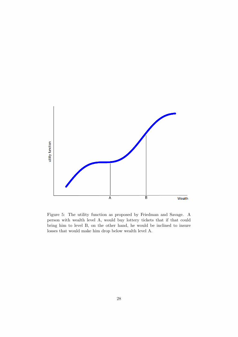
Figure 5: The utility function as proposed by Friedman and Savage. Aperson with wealth level A, would buy lottery tickets that if that couldbring him to level B, on the other hand, he would be inclined to insurelosses that would make him drop below wealth level A.

28

-risk(σ)

6return(R)

vA

BC

D

Figure 6: Two parameter criteria try to find a ranking of possible portfolios.Other portfolios compared to the one marked by the big dot are better inquadrant D because they have lower risk and higher return, in quadrant Bwe have worse portfolios (with lower return and higher risk), but those in Aand C cannot really be ranked at this level.

2.3 Rational Portfolio Theories (1950s and 1960s)

2.3.1 Modern Portfolio Theory (1952)

Markowitz introduced the “Modern Portfolio Theory” (Markowitz 1952a).The idea is as simple as powerful. The two most important criteria for aninvestment are the return and the risk. The theory of Markowitz statesthat preference should be given to a portfolio with higher return for similarrisk, or to the portfolio that has a lower risk when returns are the same.If we would plot all possible portfolios, we would get a an upper boundaryfor all portfolios. This upper boundary is called the “Efficient Frontier”,all portfolios on this frontier have this in common that there is no otherportfolio that offers both a higher return for a given amount of risk.

Markowitz suggested to use variance as a measure of risk. He did notreally argue that this would be the best choice. His line of reasoning is firstrejecting that people would/should only maximizing returns. He rejects thishypothesis (p. 77) because it leads to non-diversified portfolios.

Therefore he writes “We next consider the rule that the investor does (orshould) consider expected return a desirable thing and variance of return anundesirable thing.” and moves on proving that the “(E-V) rule” criterium(maximizing of Expected Return and minimizing Variance”). The theoryis meant as a normative theory, he writes:

“There is a rule which implies both that the investor should

29

Figure 7: The mean-variance criteria visualized for the case of 2 portfolios.Two assets are assumed with respectively return 0.15 and 0.07; and standarddeviation 0.2 and 0.1, with a correlation of 0.3.Please note that contrary to actual practice, Markowitz plotted expectedvariance on the y-axis and expected return on the x-axis.

30

diversify and that he should mazimize expected return. Therule states that the investor does (or should) diversify his fundsamong all those secutirites which give maximum expected re-turn.”– (Markowitz 1952a) - page 79.

Further on page 80 he argues that variance “is a commonly used measurefor dispersion” and that even if one uses another measure for risk than “V”such as the standard deviation or the coefficient of variation

(σR

)that then

one would find the same optimal portfolios.The essence for Markowitz is that a portfolio selection method that would

not lead to diversified portfolios (in the sense of total holdings) is unac-ceptable. Without any further claim of having found the best solution heproposes a solution that satisfies the condition of diversification and arguesthat it is wise to apply his rule because it is better than “speculative be-havior” (p. 87), because it “implies the right kind of diversfication for theright reason.”.

He mentions however a few conditions for his theory to be applicable.

“Two conditions –at least– must be satisfied before it wouldbe practical to use efficient surfaces in the manner describedabove. First, the investor must desire to act according to theE-V maxim. Second, we must be able to arrive at reasonable µiand σij”– (Markowitz 1952a) - page 83.

A Mathematical Formulation of the MV-criterion. We will fromnow on use the more popular notation “MV-criterion” in stead of Markowitzown suggestion “(E-V) rule”.

The standard deviation of a real-valued random variable X is defined as:

σ =√V AR (13)

=√E[(X − E[X])2] (definition of variance)

=√E[X2]− (E[X])2 (14)

=

√∫<

(x− µ) f(x) dx (for continuous distributions)

=

√√√√ 1

N

N∑k=1

(xk − x)2 (for discrete distributions)

with:

µ =

∫< x f(x) dx

x = 1N

∑Nk=1 xk

31

Figure 8: This figure shows possible portfolios that consist of three assets.Portfolios are plotted with a 1% step in compositions each. Once there aremore than 2 assets, the number of possible portflios explode and generallycover a surface in the (σ,R)-plane. One also sees that the portfolios withthe lowest variance include all assets. Or in other words, adding any assetthat is not 100% correlated allows us to reduce volatility for a fixed return.

A simple mathematical formulation of the mean variance optimizationcould be the following18.

Suppose that we want to construct a portfolio comprising of N possiblerisky assets. A portfolio can be referred to via the weights over the differentassets:

w = (w1, w2, . . . , wN )′

with conditionN∑i=1

wi = 1 (15)

The returns of the possible assets R = (R1, R2, . . . , RN )′, have expectedreturns µ = (µ1, µ2, . . . , µN )′ and have an expected covariance matrix de-

18Please note that this part does not follow Markowitz’ formulation, that was rathergeometrical and was limited to 3 possible assets. This formulation is more general, butuses exactly the same principles.

32

fined by:

Σ =

σ11 · · · σ1N...

...σN1 · · · σNN

Where σij is the covariance between asset i and asset j.19

Using this formulation, it is trivial that the return, expected return andexpected variance of a portfolio p are respectively defined by:

Rp = w′.R

µp = w′.µ

σ2p = w′.Σ.w

The mean variance criterion as developed by Markowitz is now reducedto

minww′.Σ.wmaxww′.µ

(16)

with constraint:w′.ı = 1 (17)

with: ı′ = (1, 1, . . . , 1)However 16 is a problem that leads to an infinite set of solutions that

cannot be ordered by these two criteria: all the portfolios on the the “efficientborder”.

We will therefore choose one:

µ0 = w′.µ

Hence we replace 16 with constraint 17 by:

minww′.Σ.w (18)

with constraints: µ0 = w′.µw′.ı = 1

(19)

This formulation of the mean variance criterion is generally referred to as“the risk minimization formulation”. It is a quadratic optimization problemwith equality restraints and is hence solved by using e.g. the method ofLagrange Multipliers.

It’s solution is given by:

w =1

a c− b2Σ−1 (cı− bµ+ (aµ− bı)µ0)

19Please note that σii = σ2i , and that in general σij = ρijσiσj .

33

where the scalars a, b and c are defined by:

a =ı′.Σ−1.ı

b =ı′.Σ−1.µ

c =µ′.Σ−1.µ

Of course one can also choose alternative formulations of the mean vari-ance hypothesis, such as the “expected return maximization formulation”or even the “risk aversion formulation”.

A most interesting and theoretically very satisfying corollary of this the-ory is that volatility aversion of the investor can be expressed by a simpleutility function where one parameter d characterizes the variance aversion.

UMPT = µ− σ2

d(20)

2.3.2 Markowitz’ Customary Wealth Theory (1952)

Markowitz published in 1952 besides the article in which he introduced hisMean Variance Theory also another article entitled “The Utility of Wealth”(Markowitz 1952b). In this publication, Markowitz explained the paradoxof Friedman and Savage (Friedman and Savage 1948) by noting that peopleaspire to move up from their current social class or “customary wealth”20.So, people might accept lottery-like odds in the hope of winning amountsthat significantly exceed their customary wealth, especially if the amountsthat can be lost are small (relative to the customary wealth level).

Considering the the utility function as proposed by Friedman and Sav-age in Figure 9 on page 35, Markowitz remarks the following discrepanciesFriedman Savage hypothesis and “common observation”, or

“behavior which not only is not observed but would generally beconsidered peculiar if it were. At other points on the curve thehypothesis implies less peculiar but still questionable behavior.At only one region of the curve the F-S hypothesis implies be-havior which is commonly observed. This in itself may suggesthow the analysis should be modified.”– (Markowitz 1952b) - page 152.

In the enumeration below, the names of Wealth levels A, B, C and D areclarified in Figure 9 on page 35.

20The “Customary Wealth” is the level of wealth to which one is used. Windfall lossesor gains might to some extend be added to the actual wealth level in order to obtain thecustomary wealth. In absence of windfall gains or losses, the customary wealth equals theactual wealth levels to which one got used.

34

Figure 9: The utility function as proposed by Friedman and Savage, withsome additional annotations.

Persons with wealth centrally between C and D should according tothe Friedman Savage hypothesis be willing to take large symmetricalbets (that allow them for example to reach D or C with equal odds.Such behaviour is not observed.

A person with wealth almost equal do D (a person that is “almostrich”, would be willing -according to the Friedman Savage hypothesis-to take a small chance of a large loss (bringing him down do C), but ifwon would rise him to D. Furthermore he would not insure against aloss that would bring him down to wealth level C. Indeed, a moderatelywealthy person that is willing to risk a large fraction of his or herwealth at actuarially unfair odds “will arise very rarely. Yet such awillingness is implied by a utility function like [Figure 9 on this page]”(Markowitz 1952b).

A person with wealth less than C or more than D will never take afair bet according to the Friedman Savage hypothesis. It is on thecontrary observed that also poor people buy lottery tickets and richpeople gamble.

One does however find that the Friedman Savage hypothesis generatequite plausible results for people that are close to wealth level A. This to-

35

gether with a series of questions to what extend one would accept gamblesor go for the sure thing, lead us to the customary wealth hypothesis.21 Thismeans that the wealth level A in Figure 9 on this page always correspondsto the present wealth.

This and some additional considerations such as

1. generally people avoid symmetrical bets, hence the utility functionmust decrease faster left from point A than it increases right frompoint A,

2. in order to avoid the St. Peterburg’s Paradox the utility functionshould be bounded from above and from below,

lead Markowitz to postulate the utility function similar to the one presentedin Figure 10 on page 37, where without loss of generality the customarywealth level is put equal to zero.

The level of customary wealth is, according to Markowitz, generally equalto the actual wealth, but can be distorted by recent windfall gains (or losses).This observation is of great importance and its impact should not be under-estimated. This implies that one will constantly update his utility functionas his wealth increases or decreases: the utility function is not a constantfunction, it changes as one advances in life.

This last observation is the essence of the hypothesis proposed by DeBrouwer and Van den Spiegel in their solution for the “Fallacy of LargeNumbers Paradox”.22 However this similarity was not noticed by the au-thors at that time.

Despite Markowitz’ own observation that his theory is only a “smallmodification of the Friedman-Savage analysis” (Markowitz 1952b), the Cus-tomary Wealth Theory is a leap forward compared to the utility functionproposed by Friedman and Savage (Friedman and Savage 1948). A funda-mental and major contribution is the fact that a utility is a quite changeableconcept for an individual, and strongly linked to what the person alreadyhas attained in his or her life (Please not the similarity with framing andloss aversion). The utility function is not longer a constant function for anindividual.

This work of Markowitz in 1952 is the foundation for Kahneman andTversky’s Prospect Theory (see (Kahneman and Tversky 1979)), Lopez’s

21Markowitz observed that people generally would prefer gambles when the lowest pos-sible outcome is small compared to the actual wealth level, but when this lowest outcomeis of a similar order or larger than the actual wealth level, then people tend to prefer thesure thing. For example one prefers a chance one out of ten to earn $1, but prefers to get$1,000,000 for sure in stead of a one out of ten probability to get $10.000.000. Similarlywhen losses are involved Markowitz found similar behaviour: risk seeking for small losses,risk averting for big losses.

22See Chapter 2.3.9 on page 49, Chapter 2.6.13 on page 71 and (De Brouwer and Vanden Spiegel 2001)

36

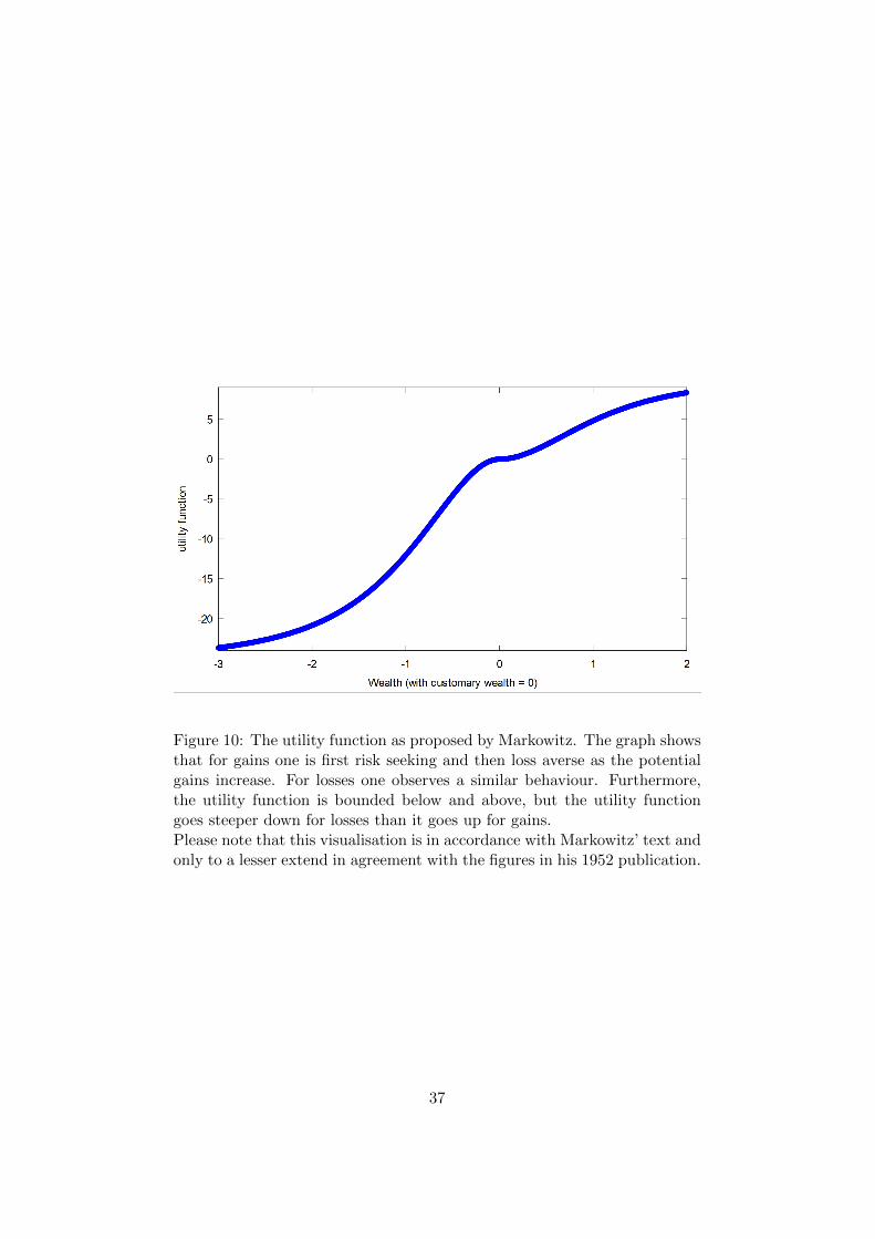
Figure 10: The utility function as proposed by Markowitz. The graph showsthat for gains one is first risk seeking and then loss averse as the potentialgains increase. For losses one observes a similar behaviour. Furthermore,the utility function is bounded below and above, but the utility functiongoes steeper down for losses than it goes up for gains.Please note that this visualisation is in accordance with Markowitz’ text andonly to a lesser extend in agreement with the figures in his 1952 publication.

37

SP/A theory (see (Lopez 1987)) as well as Shefrin and Statman’s BehaviouralPortfolio Theory (see (Shefrin and Statman 2000)). On top of that Markowitzgave here a first description of the heuristics in human behaviour that laterwould become known as loss aversion (see (Tversky and Kahneman 1991))and framing (see (Tversky and Kahneman 1981)).

Also noteworthy are the facts that Markowitz utility function allows forloss aversion rather than “volatility aversion” and that he remembers us touse bounded utility functions.

2.3.3 Roy’s Safety First Portfolio Theory (1952)

Roy argues that

“in calling in a utility function . . . , an appearance of generalityis achieved at the cost of a loss of practical significance... A manwho seeks advice about his actions will not be grateful for thesuggestion that he maximize expected utility.”– (Roy 1952)

Instead, Roy argues that investors strive to minimize the probability ofportfolio return falling below a subjectively designated disaster level. Thisbehavioural maxim is referred to as the Safety First principle. This principlecould be summarized as follows. Let’s note the return of the portfolio Rpand the minimal desired return Rm (the returns that would bring the wealthdown to the subsistence levelWs, then the Safety First Principle is equivalentto:

minpP (Rp < Rm) (21)

If returns are normally distributed, then Roy’s Safety First Principle canbe reduced to maximizing the “Safety First Ratio” (SF-ratio henceforth).

maxSF-ratio ⇔ maxE[Rp]−Rmσp

(22)

(with R[Rp] the expected return of the portfolio and σp its standard devia-tion)

One will notice that this criterion will select the same portfolios asmaximizing the Sharpe Ratio when returns are independently normally dis-tributed.

If we focus on the case where no risk free asset exists (i.e. σp > 0 : ∀p ∈P), where P is the set of all possible (acceptable)23 portfolios for a certaininvestor and/or investment problem. Also Roy focussed on the case where

23Typical restrictions would be no short selling, no derivatives, only liquid equities, onlyequities from certain countries/sectors, only bonds in certain currencies, etc. This can bethe result of the investors preference, legal framework, or what is reasonably possible oraccessible as well as costs involved in acquiring certain assets.

38

no risk free asset exist, and it is a quite reasonable assumption: there are noinvestments that have a zero variance over time horizons that are relevantfor investments (multiple years to decades).

Figure 11: This graph illustrate how optimal portfolios could be determinedfor the Safety First portfolio theory. One will notice that depending on thelevel of the required minimal return (originally called subsistence level) anyof the efficient portfolios in the sense of Markowitz can be selected. From theportfolio with the minimal variance in the limit where Rm tends to −∞ tothe portfolio that is 100% composed of the most risky assset that is selectedRm ≥ Rmax.The same two assets are considred as in Figure 7 on page 30.

In order to find the iso-SF curves in the (µp, σp) − plane we rewrite 21for a certain SF level SF0.

µp = SF0.σp +Rm (23)

So, one will notice that the iso-SF-curves are straight lines in the (µp, σp)−plane that intersect the y-axis in Rm. Of course we remember that this isonly valid in the case that portfolio returns are normally distributed so thatwe could reduce equation 21 to 22.

Later there have been some interesting generalizations of the SF PortfolioTheory.

(Tesler 1955) generalized the Safety First portfolio theory by intro-ducing a desired probability level (α) connected to the violation of the

39

minimal return. So, an investor will choose a portfolio that maximizesexpected wealth (E[W ]), subject to the constraint P (W ≤Ws) ≤ α.

(Arzac and Bawa 1977) extend Tesler’s model by allowing the prob-ability level α to vary. In that case, the expected utility functionbecomes

EU = E[W ]− c.P (W ≤Ws) (24)

= E[W ]− cDR(WS) (25)

with c a scalar, and DR(WS) the decumulative distribution function.Markowitz (Markowitz 1959) agreed that this was the only functionalform that was consistent with the expected utility hypothesis.

(Elton and Gruber 1996) discuss some generalizations, a.o. the exten-sion presented from Kataoka. Kataoka proposes that it is an investorsaim to maximize the subsistence level subject to the constraint thatthe probability that wealth falls below the subsistence level does notexceed a predetermined α.

2.3.4 The Allais Paradox (1953)

The Allais paradox is a choice problem designed by Maurice Allais to showan inconsistency of actual observed choices with the predictions of expectedutility theory. The problem arises when comparing participants’ choicesin two different experiments, each of which consists of a choice betweentwo gambles, A and B (Allais 1953). The pay-offs for each gamble in eachexperiment are as follows:

Experiment 1

– gamble 1A: 100% chance to win ¿ 1 mln.

– gamble 1B: 1% chance to win nothing + 89% to win ¿ 1 mln. +10% chance to win ¿ 5 mln.

Experiment 2

– gamble 2A: 89% chance to win nothing + 11% chance to win ¿ 1mln.

– gamble 2B: 90% chance to win nothing + 10% to win ¿ 5 mln.

The expected value (or average earnings per gamble are):

Experiment 1

– gamble 1A: ¿ 1,000,000

– gamble 1B: ¿ 1,390,000

40

Experiment 2

– gamble 2A: ¿ 110,000

– gamble 2B: ¿ 500,000

The Allais paradox lays herein that generally people prefer 1A over 1Bwhile in experiment 2 they prefer 2B over 2A. Indeed, if one prefers 1A to1B and 2B to 2A, we can write that the expected utilities of the preferredis greater than the expected utilities of the second choices (using the valuesabove and a utility function of U(W ), where W is (additional) wealth, wecan demonstrate exactly how the paradox manifests):

1.00U(106) > 0.01U(0) + 0.89U(106) + 0.1U(5.106)(experiment 1)

0.89U(0) + 0.11U(106) < 0.9 U(0) + 0.1 U(5.106) (experiment 2)

We can rewrite the equation for experiment 2 as:

⇔ 0.11 U(106) < 0.01 U(0) + 0.1 U(5.106)

⇔ 1U (106)− 0.89U(106) < 0.01U(0) + 0.1U(5.106)

⇔ 1U (106) < 0.01U(0) + 0.1U(5.106) + 0.89U(106)

which contradicts the first bet.Allais presented his paradox as a counterexample to the independence

axiom (also known as the “sure thing principle” of expected utility theory).24

2.3.5 Subjective Expected Utility Theory (SEU) (1954)

A year later Leonard Savage proposed the “Subjective Utility Theory” (Sav-age 1954). It combines two distinct subjective concepts: a personal utilityfunction and a personal probability analysis based on Bayesian probabilitytheory.

Savage proved that, if one adheres to the axioms of rationality25, and ifone believes that an uncertain event has possible outcomes ωk each witha utility to you of U(ωk) then your choices can be explained as arising froma function in which you believe that there is a subjective probability of eachoutcome is P (ωk), and your subjective expected utility is the expected valueof the utility,

EU =

N∑k=1

U(ωk).P (ωk). (26)

24Please note the similarity to the concept “framing” (Tversky and Kahneman 1981)that was not yet defined at that moment.

25This refers to a set of rationality axioms that was proved to be sufficient in order todescribe a preference relation by a utility function, see (von Neumann and Morgenstern1944).

41

You may be able to make a decision which changes the possible outcomesto ωl in which case your subjective expected utility will become

SEU =

N∑l=1

U(ωl).P (ωl). (27)

Which decision you prefer depends on which subjective expected utility ishigher. Different people may make different decisions because they mayhave different utility functions or different beliefs about the probabilities ofdifferent outcomes.

Savage assumed that it was possible to take convex combinations ofdecisions and that preferences would be preserved. So if you prefer ωk to ωland ωm to ωn then you will prefer aωk + (1− a)ωm to aωl + (1− a)ωn, for0 < a < 1.

Experiments have shown that many individuals do not behave in a man-ner consistent with subjective expected utility, most prominently (Allais1953) and (Ellsberg 1961). Savage’s response was not that this showed aflaw in his method, rather that applying his method allowed individuals toimprove their decision making.

2.3.6 cognitive dissonance (1956)

In 1956, Leon Festinger introduced a new concept in social psychology: “cog-nitive dissonance” (Festinger, Riecken, and Schachter 1956). The idea is thatwhen two simultaneously cognitions held by one person are inconsistent thatthis will produce a state of cognitive dissonance. This state produces an un-pleasant feeling that will challenge our mind and will lead to changing ofour believes (one of the two cognitions will be considered as wrong).

2.3.7 The Ellsberg Paradox popularized by Daniel Ellsberg (1961)

The Ellsberg Paradox further demonstrates how people’s choices violate theexpected utility hypothesis, even in the formulation of SEU. This paradox isnamed after Daniel Ellsberg who has the merit to popularize this paradox,but it was described earlier by John Maynard Keynes, and is described inthis text in Chapter 2.2.3 on page 9.

2.3.8 The Capital Asset Pricing Model (CAPM – 1961)

The “Sharpe-Linter-Mossin mean-variance equilibrium model of exchange”,better known as the Capital Asset Pricing Model (CAPM) is used to de-termine a theoretically appropriate required rate of return of an asset (ifthat asset is to be added to an already well-diversified portfolio) in functionthat asset’s non-diversifiable risk. The model takes into account the asset’ssensitivity to non-diversifiable risk (also known as systemic risk or market

42

risk), often represented by the quantity beta (β) in the financial industry,as well as the expected return of the market and the expected return of atheoretical risk-free asset.

The model was introduced independently by

1. Jack Treynor: (Treynor 1961) and (Treynor 1962),

2. William Sharpe: (Sharpe 1964), and

3. John Lintner and Jan Mossin: (Mossin 1966).

All authors were building on the earlier work of Harry Markowitz aboutdiversification and his Mean Variance Theory.26

The CAPM is a model for pricing an individual security or a portfolio.For individual securities, we make use of the security market line (SML)and its relation to expected return and systemic risk (beta) to show how themarket must price individual securities in relation to their security risk class.The SML enables us to calculate the reward-to-risk ratio for any security inrelation to that of the overall market. Therefore, when the expected rateof return for any security is deflated by its beta coefficient, the reward-to-risk ratio for any individual security in the market is equal to the marketreward-to-risk ratio. So we can write for an arbitrary security k:

E[Rk]−RRFβk

= E[RM ]−RRF (28)

The market reward-to-risk ratio is effectively the market risk premium andby rearranging the above equation and solving for E(Rk), we obtain theCapital Asset Pricing Model (CAPM).

E[Rk] = RRF + βk(E[RM ]−RRF ) (29)

Where:

E[Rk] is the expected return on the capital asset

RRF is the risk-free rate of interest such as interest arising fromgovernment bonds

βk (the beta coefficient) is the sensitivity of the asset returns to

market returns, or also βk = Cov(Rk,RM )Var(RM ) ,

E[RM ] is the expected return of the market

E[RM ] − RRF is sometimes known as the market premium or riskpremium (the difference between the expected market rate of returnand the risk-free rate of return).

26Sharpe received the Nobel Memorial Prize in Economics (jointly with Markowitz andMerton Miller) for this contribution to the field of financial economics.

43

Restated, in terms of risk premium, we find that:

E[Rk]−RRF = βk(E[RM ]−RRF ) (30)

which states that the individual risk premium equals the market premiumtimes beta.

Generally, the expected market rate of return is measured by looking atthe arithmetic average of the historical returns on a market portfolio (e.g.S&P 500 or DJ EurostoXX 50).

The risk free rate of return used for determining the risk premium, isusually the arithmetic average of historical risk free rates of return and notthe current risk free rate of return for the given time horizon.

Risk and Diversification The risk of a portfolio comprises systematicrisk, also known as undiversifiable risk, and unsystematic risk which is alsoknown as idiosyncratic risk or diversifiable risk. Unsystematic risk is therisk associated with individual assets, and systematic risk refers to the riskcommon to all securities (the so called market risk). Unsystematic risk canbe reduced by diversifying the portfolio by including a greater number ofassets (specific risks “average out”). systematic risk within one market cannot be diversified away, it is inherent to the market considered.

A rational investor should not take on any diversifiable risk, as they areavoidable and only non-diversifiable risks are rewarded within this model.Therefore, the required return on an asset (i.e. the return that compen-sates for risk taken), must be linked to its riskiness in a portfolio context -i.e. its contribution to overall portfolio riskiness - as opposed to its “standalone riskiness.” In the CAPM portfolio risk is represented by variance. Inother words the beta of the portfolio is the defining factor in rewarding thesystematic exposure taken by an investor.

The (Markowitz) efficient frontier and the Market Portfolio TheCAPM assumes that the volatility-return profile of a portfolio can be opti-mized: an optimal portfolio displays the lowest possible level of volatility forits level of return. Additionally, since each additional asset introduced intoa portfolio further diversifies the portfolio, the optimal portfolio must com-prise every asset, (assuming no trading costs) with each asset value-weightedto achieve the above (assuming that any asset is infinitely divisible). All suchoptimal portfolios, i.e., one for each level of return, comprise the efficientfrontier.

Because the unsystematic risk is diversifiable, the total risk of a portfoliocan be viewed as beta.

An investor might choose to invest a proportion of his or her wealth ina portfolio of risky assets with the remainder in cash - earning interest atthe risk free rate (or indeed may borrow money to fund his or her purchase

44

of risky assets in which case there is a negative cash weighting). Here, theratio of risky assets to risk free asset does not determine overall return -this relationship is clearly linear. It is thus possible to achieve a particularreturn in one of two ways:

1. By investing all of one’s wealth in a risky portfolio,

2. or by investing a proportion in a risky portfolio and the remainder incash (either borrowed or invested).

Figure 12: In this graph 100 portfolios are plotted composed out of 2 assets(increments of 1% in composition) and the Capital Allocation Line is drawn.One can observe how CAPM implies that the optimal portfolios are on theline through (0, RRF ) and pM .The same two assets as in Figure 7 on page 30 are used.

For a given level of return, however, only one of these portfolios willbe optimal (in the sense of lowest risk). Since the risk free asset is, bydefinition, uncorrelated with any other asset, option 2 will generally havethe lower variance and hence be the more efficient of the two.

This relationship also holds for portfolios along the efficient frontier:a higher return portfolio plus cash is more efficient than a lower returnportfolio alone for that lower level of return. For a given risk free rate, thereis only one optimal portfolio which can be combined with cash to achievethe lowest level of risk for any possible return. This is the market portfolio(pM ).

45

Assumptions of CAPM All Investors:

1. try to maximize utility,

2. are rational and volatility-averse,

3. are price takers, i.e., they cannot influence prices.

4. are able to lend and borrow under the risk free rate of interest withno limitations,

5. trade without transaction costs,

6. are not taxed in any way on their investments or transactions,

7. deal with securities that are all highly divisible into small units,

8. assume all information is at the same time available to all investors.

Shortcomings of CAPM Despite its theoretical appeal and its coherencewith other theories for rational behaviour, such as expected utility theory,CAPM has many weak points.

1. CAPM assumes that asset returns are (jointly) normally distributedrandom variables. However this is (despite the Central Limit Theorem)an oversimplification that is unable to capture exactly those eventsthat are of interest.27

2. The model assumes that the standard deviation (or variance) of returnsis an adequate measurement of risk. Risk in financial markets is notvolatility, it is the probability of losing. The risk is a downside riskand not the upside potential.28

3. CAPM assumes that there exists something as “expected return” inthat sense that investors agree about it (homogeneous expectationsassumption).

27Indeed, the Central Limit Theorem states that the sum of identically distributedrandom variables will tend to a Gaussian distribution, but that convergence is weak andonly valid in the centre of the distribution. Financial risks are exactly those extremeevents “in the tails of the distribution”. In the literature are many references to statisticaldistributions in finance, one of the most successful distributions in capturing observationsare the Levy distributions, and according to the author one of the best works describingthis is (Bouchaud and Potters 1997).

28Much more relevant measures of risk can be defined such as Value at Risk, downsidevolatility, maximal drawdawn, longest period of loss, etc. Once more a good source is(Bouchaud and Potters 1997).

46

4. CAPM assumes that the beliefs of investors about the probabilitiesmatch the true distribution of returns. Also this is widely studied anddoes not hold.29

5. CAPM does not appear to adequately explain the variation in stockreturns. Empirical studies show that low beta stocks may offer higherreturns than the model would predict; for example see (Black, Jensen,and Scholes 1972) find that “high beta” stocks on average earn lessthan the model predicts and “low beta stocks” earn more. Some datawas presented as early as a 1969 conference in Buffalo, New York.Either these findings are rational (which saves the efficient-market hy-pothesis but makes CAPM wrong), or it is irrational (which savesCAPM as a theoretical model, but makes the EMH wrong; this possi-bility makes volatility arbitrage a possible strategy for systhematicallybeating the market).

6. CAPM assumes that given a certain expected return investors willprefer lower risk (lower variance) to higher risk and conversely givena certain level of risk will prefer higher returns to lower ones. It doesnot allow for investors who will accept lower returns for higher risk.Casino gamblers clearly pay for risk, and it is possible that some stocktraders will pay for risk as well.

7. CAPM assumes that there are no taxes or transaction costs, althoughthis assumption may be relaxed with more complicated versions of themodel.

8. The market portfolio consists of all assets in all markets, where eachasset is weighted by its market capitalization. This assumes no pref-erence between markets and assets for individual investors (such ashome bias), and that investors choose assets solely as a function oftheir risk-return profile. It also assumes that all assets are infinitelydivisible as to the amount which may be held or transacted.

9. The market portfolio should in theory include all types of assets thatare held by anyone as an investment (including works of art, real estate,human capital...) In practice, such a market portfolio is unobservableand people usually substitute a stock index as a proxy for the true mar-ket portfolio. Unfortunately, this substitution can lead to underminesthe validity of the CAPM. Further, due to the inobservability of thetrue market portfolio the CAPM might not be empirically testable.This was presented in greater depth in a paper by Richard Roll in1977, and is generally referred to as Roll’s critique. See (Roll 1977).

29See for example the overconfidence-based asset pricing model of Kent Daniel, DavidHirshleifer, and Avanidhar Subrahmanyam (Daniel, Hirshleifer, and Subrahmanyam2001).

47

10. CAPM assumes that investment decisions are made by taking justtwo dates into account, so that there is no opportunity to consumeand rebalance portfolios repeatedly over time.

11. CAPM assumes that all investors will consider all of their assets andoptimize one portfolio. This is in sharp contradiction with portfoliosthat are held by investors. People tend to have separate portfolios forseparate goals (retirement, education for children, special expenses,etc.)

Some Definitions

CML Capital Market Line. The line that connects (RRF , 0) and themarket portfolio. All portfolios on the CML are those in which, ac-cording to CAPM an investor should invest. It’s equation is:

E[R] = RRF + E[σ]E[RM ]−RRF

E[σM ](31)

CAL Capital Allocation Line. The line that connects all portfolios thatcan be constructed by combining a risky portfolio (p) and the risklessasset. It’s equation is:

E[R] = RRF + E[σ]E[Rp]−RRF

E[σp](32)

In CAPM, this is the line along which the investor will move his port-folios, he will allocate more to cash if he wants a safer portfolio andmore to the risky portfolio if he seeks a more dynamic portfolio. Doingso, he will only balance cash and this portfolio, he will not change theportfolio itself (for example more into equities and less into bonds!).30.An investor, investing according to CAPM will find that his CAL isthe same as the CML.

SCL Security Characteristic Line is the line that represents the relationbetween the market return and the return of a specific asset i at a giventime interval t, it’s equation is:

Ri,t = αi + βi RM,t + εi,t (33)

Where αi and βi are referred to as respectively the “alpha and thebeta of the security i”.

30Please note that in practice advisors will generally advice more equities and less bondsif a client seeks a more dynamic investment. This is in contradiction with CAPM, and itsis called the “Asset Allocation Puzzle”, see Chapter 2.6.9 on page 66

48

SML Securities Market Line shows the expected return as a function ofβ. The intercept is the risk free rate of return RRF and the slope isE[RM −RRF ]. It’s equation is hence:

E[Ri] = RRF + βi E[RM ]−RRF (34)

The SML is actually a single factor model for the price of a given asseti, and so it can be considered as the graph that represents the resultsof the CAPM.

2.3.9 The Fallacy of Large Numbers (1963)

P. A. Samuelson builds his paradox “the fallacy of large numbers”, suggest-ing that time horizon is not relevant for investments (Samuelson 1963).

“that a person whose utility schedule prevents him from evertaking a specific favourable bet when offered only once can neverrationally take a large sequence of such fair bets, if expectedutility is maximised”– (Samuelson 1963)

Of course “one bet” can be seen as one time unit in investing, and aseries of bets is then the longer time horizon. This is very important sincepractitioners tend to advise more risky assets on longer investment horizons.

2.3.10 The Efficient Market Hypothesis (EMH) (1964)

The efficient-market hypothesis was first expressed by Louis Bachelier, aFrench mathematician, in his 1900 dissertation, “Theorie de la speculation”(Bachelier 1900a) - also published as a book (Bachelier 1900b). His workwas largely unknown among economists till P.A. Samuelson brought it to theattention. In 1964 Bachelier’s dissertation along with the empirical studiesmentioned above were published in an anthology edited by Paul Coonter,and a year later, E. Fama published his dissertation.

The efficient-market hypothesis (EMH) states that the relevant financialmarkets are “informationally efficient”, i.e. prices on traded assets alreadyreflect all known information. The efficient-market hypothesis states that itis impossible to consistently outperform the market by using any informationthat the market already knows, except through luck.

Information or news in the EMH is defined as anything that may affectprices that is un-knowable in the present and thus appears randomly in thefuture.

The EMH was developed by Eugene Fama at the University of ChicagoBooth School of Business as an academic concept of study through his Ph.D.thesis that was published in the early 1960s. Only slowly it gained adherence,and developed a strong status both among academicians and practitioners.

49

Despite of its logical acceptance many business models in asset managementand many individuals are trying to select portfolios that outperform themarkets.

Many studies (starting with (De Bondt and Thaler 1985)) showed thatmarkets are not efficient in the sense that patterns exist. However this doesnot necessarily mean that these patterns can be exploited in order to beatthe financial markets. Indeed practitioners seem to have much more troubleto find strategies that continue to perform. Therefore even if markets are notefficient, but if we have no way to predict future patterns, it is not excludedthat the EMH is still the best approximation to be used in analysis.

Different forms of market efficiency The efficient-market hypothe-sis requires that agents have rational expectations on top of the rationalbehaviour of maximizing a utility function; that on average market is cor-rect31 and whenever new relevant information appears, the agents get it atthe same time and update their expectations appropriately and in a rationalway.

Note that it is not required that the agents are completely rational (inthe sense that they show no behavioural biases). Some investors may overre-act and some may underreact to new information. EMH only requires thatthe reactions of the investors are on average rational and correct. Individualinvestors’ reactions should be random and follow a normal distribution sothat the effect on the market prices cannot be reliably exploited (in order togenerate systematic excess return above market), especially when consider-ing transaction costs (including commissions and spreads).32

Generally three different levels (or forms) of market efficiency are con-sidered.

Weak-form efficiency

– One cannot generate excess returns by using investment strategiesbased on historical share prices.

– Technical analysis will not be able to produce systematically ex-cess returns, however some forms of fundamental analysis maystill provide excess returns.

– Asset prices do not show ”patterns”. This implies that futureprice movements are determined entirely by information not con-tained in the actual price. Hence, prices must follow a randomwalk.

31Please note that all agents on a certain market can be wrong, EMH only requires thatthe market as a whole is right (as an average).

32Hence the adagio: “the market is always right”, and “there is no such thing a freelunch”.

50

Semi-strong-form efficiency

– Share prices adjust to new public information very rapidly andin an unbiased fashion, so that no excess return can be earned bytrading on new information.

– Semi-strong efficiency implies that neither fundamental analysisnor technical analysis techniques will be able to reliably produceexcess returns.

– To test for semi-strong-form efficiency, the adjustments to previ-ously unknown news must be of a reasonable size and must beinstantaneous. To test for this, consistent upward or downwardadjustments after the initial change must be looked for. If thereare any such adjustments it would suggest that investors had in-terpreted the information in a biased fashion and hence in aninefficient manner.

Strong-form efficiency

– Share prices reflect all information, public and private, and noone can earn excess returns.

– If there are legal barriers to private information becoming public,as with insider trading laws, strong-form efficiency is impossible,except in the case where the laws are universally ignored.

– To test for strong-form efficiency, one would test investor’s out-perfomance: no investors should be able to systematically out-perform the market.33

2.3.11 Models for Lifetime Portfolio Selection - 1968 and 1969

There was some literature available about portfolio slection when more thanone time horizon is involved. The first multi period analysis is from (Phelps1962) and (Tobin 1965), whereas (Mossin 1968) made the first attempt toextend the existing portfolio selection methods from one period to multipleperiods. In August 1969 Paul A. Samuelson and Robert C. Merton publishedboth in The Review of Economics and Statistics a paper about lifetimeportfolio selection. (Samuelson 1969) derived the equations that govern thechoice between consumption, a risky asset and a non-risky asset in “LifetimePortfolio Selection by Dynamic Stochastic Programming” for the discretecase. (Merton 1969) did the same for the continous-time case in “LifetimePortfolio Selection Under Uncertainty: the Continuous Time Case”.

33Please note that a normal distribution of a large group of managers will indeed showsome lucky “star performers”. In order to reject the strong-form market efficiency, onewould have to find more star performers than a normal distribution would predict.

51

Samuelson assumes that the individual tries (or should try) to maximize∫ T0 eρtU(C(t)) dt, where C(t) is the consumption and rho is the continuous

time interest rate at which can be invested and that one has a chocie betweena riskless asset and a risky asset whose return is governed by a Wienerprocess34. Then he studies the calculus-of-variation problem resulting fromthis in the continous time case. and hence maximizes

MaxCt, wt

E

[T∑t=0

(1 + ρ)−tU(Ct)

]

with the condition that Ct = Wt− Wt+1

(1+r)(1−wt)+wtZt . r is the interest rate atwhich one can invest in the save asset and wt is the raction of the portfolioinvested in the risky asset, and Zt is the return of the risky assset in theperiod t.

Samuelson demonstrates that in the case of isoelastic utlity functions(such as U = logC)35 the problem can be solved and in that case the“business man risk” is a fallacy, or otherwise stated: age in itself does notinfluence the risk profile. Isoelastic utility functions are problematic for theKarl Menger paradox, but in all other cases wT−j becomes a function ofWT−j−1 and the equations are till now a challenge.

Merton finds that in the same problem (and with the same notations)for in the two asset case is determined by

MaxC,w

Φ(w,C;W ; t)

Where

Φ ≡ e−ρtU(C)∂It∂t + ∂It∂W [(w(t)(a− r) + r)W (t)− C(t)]

+12∂2I∂W 2σ

2w2(t)W 2(t)

In this equation It is used as a shorthand notation for I(W (t), t), that isdefined as

I(W (t), t) ≡ MaxC(s), w(s)

E(t)

[∫ T

te−ρsU(C(s)) ds+B(W (T ), T )

]34A Wiener process (named after Norbert Wiener is another word for to describe Brown-

ian Motion. Essential in its definition is that the system has no memory (therfore all stepsare independent from the previous ones) and that each step is governed by a Gaussian dis-tribution. De assumption of a independently distributed returns following a MultivariateNormal Distribution is an significant simplification of reality.

35An iso-elastic utlity function is a utility funcition that dislpays constant relative riskaversion, Merton will call this “iso-elastic marginal utility”. Generally functions of theform Cγ

γ(with γ 6= 0 and γ < 1) display this property, and of course logC, the limit

case with γ = 0. For such functions we find indeed that Pratt’s measure for relative risk

aversion (see (Pratt 1964)),∂2U∂C2∂U∂C

C, is a constant (1− γ).

52

Wher E(t) is the conditional expected value operator (conditional to theknowledge of W (t)

The necessary first order conditions are then a system of nonlinear partialdifferntial equations coupled with two algebraic equations. Such equationsare hard to solve, it is only in the 1970s and 1980s that the true natureof such equions was explored more in debt by physicists in their searchto understand complex nonlinear systems, see our chapter about “ChaosTheory”, Chapter 2.2.4 on page 10. The book “Strategic Asset Allocation:Portfolio Choice for Long-Term Investors” (Campbell and Viceira 2002) iscompletely dedicated to approximated solutions of a simplified form of thisequation.

Merton confirms Samuelson’s findings that for iso-elastic marginal utilitythe portfolio selection decission is independent of the consumption decission.In case of log-utility the consumption decission only depends on the level ofwealth.

2.3.12 An Intertemporal Capital Asset Pricing Model - 1973

In 1973 Robert C. Merton (Merton 1973) uses these findings to develop anintertemporal model for the capital market. The central idea is to write anIto equation for the capital market.

dX = F (X) dt+G(X) dQ

Where X is the vecotor composed of prices, return and covariances, G(.) adiagonal matrix and dQ the Wiener process.

The model requires knowledge of many parpameters about all companiesand investors and 10 assumptions (including all the assumptions needed forthe CAPM) are required.

An interesting result from this model is that there are only two optimalportfolios: the riskless asset and another (market) portfolio. All investorsshould hence hold a combination of those two.

The model is enourmously complex and impossible to integrate, but itstill does not include wage income and many consumption goods whoseprices can change over time.

This model of Merton was another important step and many authorsworked further on this model. See for example (Breeden 1979), who triedto simplify the beta and allow for stochastic consumption.

2.4 Upcoming challengers from Psychology: the 1970s andthe early 1980s

2.4.1 Availability Heuristic (1973)

Tversky and Kahneman introduced the concept: “availability heuristic”.They found that our mind constantly uses the availability bias:

53

“The availability heuristic is a judgemental heuristic in whicha person evaluates the frequency of classes or the probabilityof events by availability, i.e. by the ease with which relevantinstances come to our mind.”– (Tversky and Kahneman 1973)

Another way to view this is stating that when one has to make a decision,one will be inclined to use knowledge that is already available rather thanexamine other (more relevant) alternatives.

2.4.2 More Heuristics (1974)

A year later the same authors described three heuristics that are used whenmaking decisions when outcomes are uncertain (i.e. under uncertainty)(Tversky and ne man 1974).

Representativeness. When people are asked to judge the probabilitythat an object or event A belongs to class or process B, probabilitiesare evaluated by the degree of which A is representative of B (that isby the degree A resembles B)

Availability. When people are asked to asses the frequency of a classor the probability of an event, they do so by the ease with whichinstances or occurrences can be brought to mind. In other words,when something is fresh in our mind, it appears to us that it is moreprobable to occur than events that are less fresh in our mind. (alreadypublished in 1973)

Anchoring and adjustment. When an anchor36 is available, peoplemake estimates by starting from the initial value of the anchor. Theanchor may be suggested by formulation of the problem, or it maybe the result of partial computations. In both cases the adjustmentsmade are small, and people’s guesses are strongly influenced by theanchor.

2.4.3 Support for CAPM and related theories – 1976

In the 1970s, there were hundreds of papers published that elaborate onCAPM. Mark Rubenstein wrote for example a paper dedicated to the sup-port of the Generalized Logaritmic Utility Function in 1976. He argued thatit captures most of the dynamics while still being able to handle mathemat-ically. – (Rubinstein 1976a)

Later during the same year he made the link from the valuation of un-certain income streams to option pricing theory – (Rubinstein 1976b).

36An “anchor” can be almost anything that our mind uses to hold on, or to use it as astarting point to make an estimate. It might even be totally irrelevant information.

54

2.4.4 Prospect Theory (1979)

Expected Utility Theory is unable to explain the Allais Paradox nor theFriedman-Savage paradox. People underweight outcomes that are merelyprobably relatively to outcomes that are certain. Also people discard com-ponents that are shared by all gambles under consideration (see Allais Para-dox). These issues are accounted for in the theory that was constructed byKahneman and Tversky. They called their new theory “prospect theory”(Kahneman and Tversky 1979).

In prospect theory, people make decisions based on the value of gainsand losses (as opposed to the utility of total wealth), and probabilities arereplaced by decision weights. The value function is relative to a referencepoint, and is concave for gains (risk aversion) and convex for losses (riskseeking), and is generally steeper for losses than for gains (loss aversion).The decision weights are generally lower than the corresponding probabili-ties, expect in the range of low probabilities.

Figure 13: Prospect Theory assumes that human decision are not made infunction of or a utility function (with total wealth as variable), but decisionsare made in function of a value function (that plays the same role, but usesthe outcome of the gamble as variable (i.e. the incremental wealth)).

2.4.5 Framing (1981)

Tversky and Kahneman showed that decisions display predictable shiftswhen the same problem is differently framed. They called this phenomenon

55

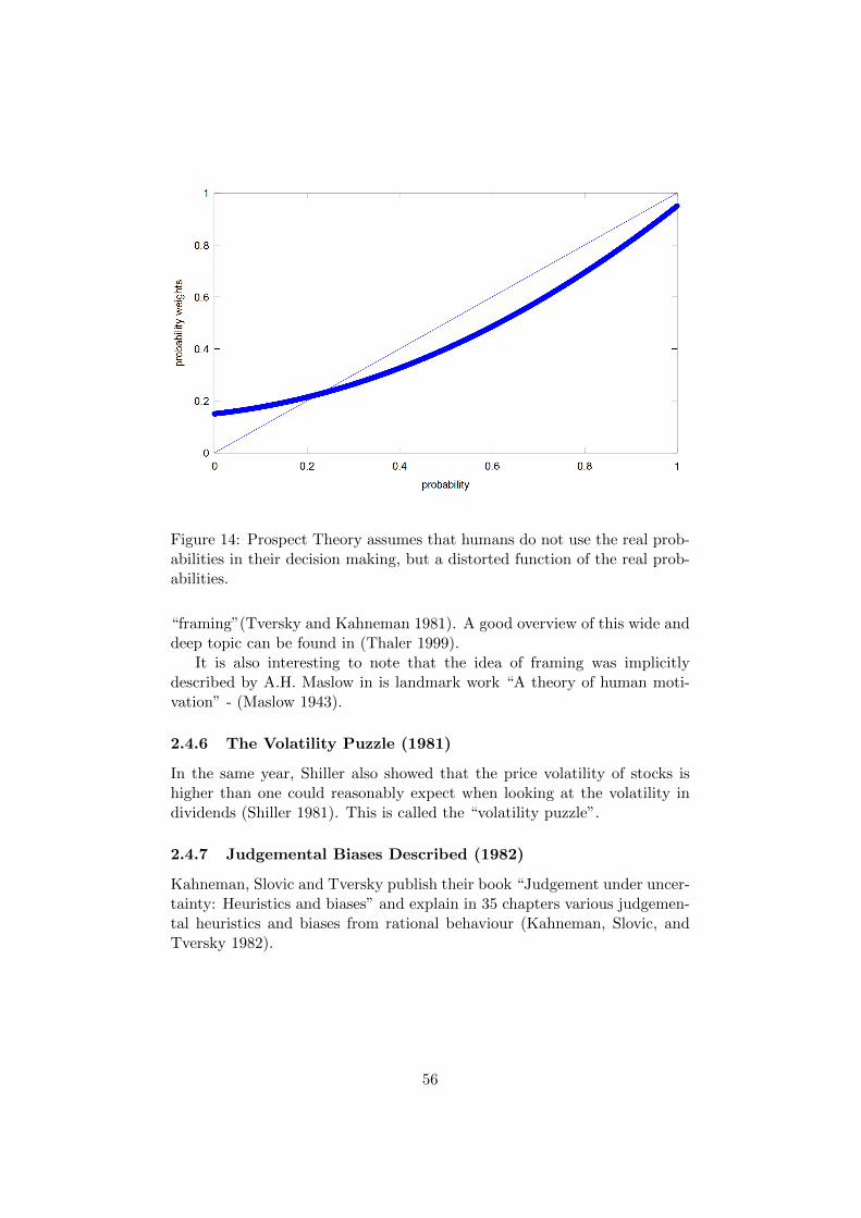
Figure 14: Prospect Theory assumes that humans do not use the real prob-abilities in their decision making, but a distorted function of the real prob-abilities.

“framing”(Tversky and Kahneman 1981). A good overview of this wide anddeep topic can be found in (Thaler 1999).

It is also interesting to note that the idea of framing was implicitlydescribed by A.H. Maslow in is landmark work “A theory of human moti-vation” - (Maslow 1943).

2.4.6 The Volatility Puzzle (1981)

In the same year, Shiller also showed that the price volatility of stocks ishigher than one could reasonably expect when looking at the volatility individends (Shiller 1981). This is called the “volatility puzzle”.

2.4.7 Judgemental Biases Described (1982)

Kahneman, Slovic and Tversky publish their book “Judgement under uncer-tainty: Heuristics and biases” and explain in 35 chapters various judgemen-tal heuristics and biases from rational behaviour (Kahneman, Slovic, andTversky 1982).

56

2.5 First Signs of Acceptance for Behavioural Finance: 1985

2.5.1 The first real evidence of market non-efficiencies

Werner De Bondt and Richard Thaler provide evidence that markets areindeed not efficient (De Bondt and Thaler 1985). In their landmark arti-cle, “Does the Stock Market Overreact?”, they show that the stock market“overreacts”, and that substantial “weak form market inefficiencies” exist.Their comparison of a portfolio of “loser stocks” with a portfolio of “winnerstocks” was so clear and undeniable that it send a shock-wave through theworld of economists. Their results were so unexpected and so profound thatthis would become a turning point in history.

Many also see this landmark article of De Bondt and Thaler as the startof “behavioural finance”, as the beginning of what is now a widely acceptedparadigm.

2.5.2 Mental Accounting

In the same year Thaler developed a new model for consumer behaviour thatwas build on “mental accounting” (Thaler 1985). This important conceptis the emanation of framing in our behaviour. People tend to distributetheir assets over different mental accounts, with each their separate goaland do not put all assets in one optimized portfolio, as the rational MPTprescribes. People have different portfolios for retirement, for children, forspecial projects,. . . and on top of that they buy lottery tickets.

This concept of mental accounting is based on framing and the Allaisparadox, and would turn out to become a cornerstone of Behavioural Port-folio Theory.

2.5.3 The Equity Premium Puzzle

The equity premium puzzle was introduced by R. Mehra and E.C. Prescott(Mehra and Prescott 1985).

“Historically the average return on equity has far exceeded theaverage return on short-term virtually default-free debt. Overthe ninety-year period 1889-1978 the average real annual yieldon the Standard and Poor 500 Index was seven percent, while theaverage yield on short-term debt was less than one percent. Thequestion addressed in this paper is whether this large differentialin average yields can be accounted for by models that abstractfrom transactions costs, liquidity constraints and other frictionsabsent in the Arrow-Debreu set-up[37]. Our finding is that it

37The Arrow-Debreu model, also known as the Arrow-Debreu-McKenzie model can beused to prove that an economic equilibrium exists where the prices are such that the

57

cannot be, at least not for the class of economies considered.Our conclusion is that most likely some equilibrium model witha friction will be the one that successfully accounts for the largeaverage equity premium.”– (Mehra and Prescott 1985)

2.6 Towards Acceptance of Behavioural Finance Among Schol-ars (1985 - 2000)

2.6.1 The late 1980s

Choice Theory. Tversky and Kahneman (Tversky and Kahneman 1986)write that due to framing and prospect theory, the rational theory of choicecannot be a good descriptive theory of human decision making.

The 93% Question. Also in 1986, Brinson et al. show that the variationof a portfolio is for 93% determined by the strategic choice of asset classes(Brinson, Hood, and Beebower 1986) and see also (Brinson, Singer, andBeebower 1991). This is a very important discovery for portfolio selection,because it indicates what portfolio selection actually is. It is all about gettingthe strategic benchmark right, i.e. the average composition of the portfolioin terms of asset classes such as shares, bonds, alternative investments, cash.All the rest such as style, geographic bias, asset manager, active or passivemanagement, etc only account for 7% of the variation.38

EUT modified for the Allais Paradox. Yaari, however, finds that EUTcan be modified to accommodate the Allais Paradox (Yaari 1987).

SP/A Theory (1987). Lopez Lola’s SP/A theory is a general frameworkfor human decision making rather than a portfolio theory, however it can beconsidered as an extension of Arzac’s Security First model.

In SP/A theory, the S stands for security, the P for potential and theA for aspiration. The concept of security is closely related to the safety inSafety First theory (avoiding low levels of wealth). Aspiration is related toa goal.39 Potential is related to the general desire to achieve higher levels ofwealth (a concept that is absent in SF-theory).

aggregate demand equals the aggregate supply. The conditions needed are: convexity,perfect competition and demand independence.This model is the fundamental model in the General (Economic) Equilibrium Theory. Themodel is named after Kenneth Arrow, Gerard Debreu and Lionel W. McKenzie

38Interesting is to note that in the USA it is common practice to pay for a financialplanning (that answers the 93% question, but in Europe the main focus is mainly on the7%.

39This can be considered as a generalization of the SF-theory, however it has necessarilydeep implications. Once we start talking about a goal, necessarily one will be confronterby the fact that humans have multiple investment goals and that the portfolio necessarily

58

In all Safety First models risk is represented by the the probability offalling below a certain subsidence wealth level, Ws. This probability isbest expressed by the complementary cumulative distribution function (ora decumulative probability function)40, D, defined as D(x) = P (W ≥ x).

Assume the discrete setting, so that after a certain horizon an invest-ment can have M different states, that occur with a probability pi so thatpi = P (Wi) ∀i ∈ 1, 2, . . . ,M. Assume without loss of generality thatthe wealth levels are ordered so that W1 ≤ W2 ≤ · · · ≤ WM . Then onewill notice that the expected wealth after the experiment equals E[W ] =∑M

i=1 piWi =∑M

i=1Di(Wi −Wi−1), with W0 = 0.41 Also one will noticethat D1 = 1, i.e. one will receive W1 with certainty, and can additionallyget W2 −W1 with a probability D2, etc.

SP/A theory now includes two aspects that influence human decisions:hope for potential and fear (or the need for security).

Fear is the human need for security and will lead to make calculationsnot with pi but with modified probabilities that overweight the probabilitiesof bad outcomes (so assume that the probability of low gains (low i) corre-sponds to higher values than the actual probabilities. This is the concernfor security and it can be formulated as follows.

hs(D) = D1+qs

where the s refers to security and with qs > 0.Hope for potential will result on the contrary in overweighting positive

outcomes (so the higher i). This hope for potential will result in SP/Atheory in another distortion of the ccdf.

hp(D) = 1−(1−D1+qp

)where the p refers to potential and with qp > 0. One will notice that becauseof the overweighting of the higher results, hp(D) will stochastically dominateD.

has to be broken down in multiple sub-portfolios. We cannot avoid to arrive finally at aportfolio theory such as Target Oriented Advice.

40The “complementary cumulative distribution function” (ccdf) is sometimes referredto as “decumulative distribution function” (ddf) or “survival function” (mainly in survivalanalysis, the discipline that studies death in biological systems or failure in mechanicalsystems). We will write the ccdf for a stochastic variable X as DX , and it is defined by

DX(x) =P (X > x)

=1− FX(x)

where FX(x) is the cumulative distribution function (cdf), defined as FX(x) = P (X ≤x) =

∫ x−∞ fX(t) dt, where f(t) is of course the probability density function (pdf).

41Please note that the subscript X is in this discussion omitted in the notation for theccdf, DX , in order not to overload the notations.

59

Then SP/A theory combines simply this need for security and hope forpotential by using the following distorted ccdf.

h(DX) = a hs (DX) + (1− a) hp (DX) (35)

The individual person presented with a decision where outcome is uncertainwill then according to SP/A theory not base his decisions on E[W ], but onEh[W ], which is obtained by replacing all probabilities pi by pi = h(Di+1)−h(Di). So, here SP/A theory differs from EUT by using a rank dependentformulation (i.e. replacing DX by h(DX).

Furthermore Lopez postulates that decisions when outcome is uncertainare based on two functions.

the modified expected wealth, Eh[W ]

D(A) = P (W > A), or the probability that the outcome will exceed acertain aspiration level.

Hence the function to evaluate possible outcomes

U = U (Eh[W ], D(A)) (36)

is a monotonous increasing function, conform the Arzac Bawa generalizationof the SF theory.

This utility function could for example be a Cobb-Douglas42 function.

USPA−CD (Eh[W ], D(A)) = (D(A))1−γ Eh[W ]γ (37)

Now, it becomes also clear how SP/A-theory could be regarded as anextension of SF-theory (where humans base their decisions on E[W ] andP (W ≤Ws)). The expected wealth is in the SP/A theory distorted by hopeand fear, and the subsistence level is that theory a more general aspirationlevel (so, it can be a disaster level such as in SF theory, but it can also beanother level). In the limit case where qs = qp = 0, the SP/A model isequivalent to the Arzac-Bawa model.

It is worth to mention here that “risk” is multidimensional in the SP/Amodel. Risk is characterized by 5 parameters.

1. qs is a measure for the strength of fear, or the need for security;

2. qp is a measure for the strength of hope, or the desire for potential;

3. A is the value of the aspiration level;

42When Cobb and Douglas introduced their functional form in (Cobb and Douglas1928), they presented it as a functional for of the production function of a company. Theproduction level is characterized by Y = A Lα Kβ , where Y represents the productionlevel, A the total factory productivity, L the labour input and K the capital input. In thespecial case where α+ β = 1, there are “constant returns of scale”.

60

4. a is a measure for the strength of fear relative to the strength of hope;

5. at least one other parameter that is a measure for the strength of thedesire to reach the aspiration level relative to fear and hope in 36.

The aspiration level A merits a closer look. The fact that the ideaof a subsistance level of wealth (such as in Roh’s Safety First theory) isabandoned in favour of an aspiration level is not a big step in itself. It doesnot exclude that there is only one aspiration level, but it at least semanticallya step closer to a problem setting with multiple goals.

Further Evidence for non rational heuristics in human decisionmaking. De Bondt and Thaler report further evidence supporting theoverreaction hypothesis (De Bondt and Thaler 1987). Samuelson and Zeck-hauser find evidence of the “status quo bias” (the tendency to prefer theomission of action over action - a heuristic that reduces future regret byhindsight) (Samuelson and Zeckhauser 1988).

2.6.2 Evidence of Analyst overreaction

De Bondt and Thaler already had presented evidence (De Bondt and Thaler1985) and (De Bondt and Thaler 1987) that financial markets overreact.However one could still expect that this was a bias caused by the non-professional investors. Therefore the same authors investigate the behaviourof professional analysts and find evidence that also they overreact (De Bondtand Thaler 1990).43 They conclude that the analysts earnings forecasts astracked by the Institutional Brokers Estimate System (IBES) are indeed“consistent with generalized overreaction”. Further they show that the earn-ing chances foretasted by the analysts are significantly more extreme thanactual realizations. They conclude that

“the earnings forecasts are simply too extreme to be consideredrational”– (De Bondt and Thaler 1990)

2.6.3 The Discussion about the Efficiency of the Stock Markets

Since J.M. Keynes’s statement that most investor’s decissions “can only betaken as a result of animal spirits – of a spontaneous urge to action ratherthan inaction, and not as the outdome of a weighted average of benefitsmultiplied by quantitative probabilities” (Keynes 1936) and the formulation

43The findings of De Bondt and Thaler are somehow questioned by (Abarbanell andBernard 1992), however also their findings and conclusions lead also to systematic devia-tions from rational behaviour for analysts. They however report both over and underre-action.

61

of the EMH many research has been devoted to the nature or the stochas-tics related to financial markets. The conclusions of Fama’s famous survey(Fama 1970) is that most of these studies are unable to rejected the “efficientmarket hypothesis”.

In 1988 Andrew Lo and Mackinlay compare variance estimators derivedfrom data sampled at different frequencies and conclude that

“The random walk model is strongly rejected for the entire sam-ple period (1962- 1985) and for all subperiod for a variety ofaggre- gate returns indexes and size-sorted portofolios. Althoughthe rejections are due largely to the behav- ior of small stocks,they cannot be attributed com- pletely to the effects of infrequenttrading or time- varying volatilities. Moreover, the rejection ofthe random walk for weekly returns does not support a mean-reverting model of asset prices. ”– (Lo and MacKinley 1988)

2.6.4 Loss Aversion and endowment effect

Kahneman et al. reported evidence that people are “loss averse” and thatthe “endowment effect”44 persists even in settings with opportunities tolearn and conclude that they are fundamental characteristics of human de-cision heuristics (Kahneman and Thaler 1990)

2.6.5 And more Contributions to the Behavioural Paradigm

Many other articles and books show that more and more scholars becomeconvinced that significant deviations from rational behaviour occur. Gilovichwrote the book “How We Know What Isn’t So”, about the failability of hu-man decision making and learning (Gilovich 1991)

Tversky and Kahneman present a reference dependent model of risklesschoice that is constructed on loss aversion (Tversky and Kahneman 1991).

Thaler publishes “The Winner’s Curse: Paradoxes and Anomalies ofEconomic Life” (Thaler 1992).

Banerjee presents a simple model of herd behaviour (Banerjee 1992).

2.6.6 Cumulative Prospect Theory (1992)

Tverky and Kahneman build further on their prospect theory and create anew version: “cumulative prospect theory” - (Tversky and Kahneman 1992).

44The endowment effect (also known as divestiture aversion) is a hypothesis that peoplevalue a good or service more once their property right to it has been established. In otherwords, people place a higher value on objects they own than objects that they do not. Inone experiment, people demanded a higher price for a coffee mug that had been given tothem but put a lower price on one they did not own.

62

It uses cumulative decision weights (and not longer the separable decisionweights), it works for certain as well as for risky prospects with any numberof outcomes, and it allows for different weighting functions for losses andgains.

Just as Prospect Theory this theory has no ambitions to be a normativetheory. It strictly seeks to describe human decision making under uncer-tainty. Its assumptions and potential are quite similar to Prospect Theory,however theoretically it is an important improvement. The main modifi-cation to Prospect Theory is that, as in rank-dependent expected utilitytheory, cumulative probabilities are transformed, rather than the probabili-ties itself. This leads to the aforementioned overweighting of extreme eventswhich occur with small probability, rather than to an overweighting of allsmall probability events. The modification helps to avoid a violation offirst order stochastic dominance and makes the generalization to arbitraryoutcome distributions easier.

This theory “predicts”:

risk aversion for gains and risk seeking behaviour for losses of highprobability, and

risk seeking for gains and risk aversion for losses of low probability.

The theory is also successful in explaining the equity premium puzzle,the endowment effect, status quo bias, asset allocation puzzle, etc.

Its basic assumptions are

Utility is a function of gains and losses not of the total final wealth.

The shape of the utility function (or value function as they call it)is convex for gains (risk averse) and concave for losses (risk seeking),with a greater sensitivity for losses than for gains (this phenomenonis also known as loss aversion, see for example (Barberis and Huang2001)).

A final aspect of the Cumulative Prospect Theory is the non-lineartransformation of probabilities.

They also reported confirming experimental evidence of their theory.

2.6.7 A Solution for the Equity Premium Puzzle (1995)

When one studies the returns of equities over the last century, and comparesthem with what EUT would predict, one finds that the risk premium is farhigher than the theory would predict. This paradox is referred to as the“equity premium puzzle”. Benartzi and Thaler proposed a solution for theequity premium puzzle based on behavioural concepts (Benartzi and Thaler

63

Figure 15: Cumulative Prospect Theory assumes (similar to Prospect The-ory) that human decision are not made in function of or a utility function(with total wealth as variable), but decisions are made in function of a valuefunction (that plays a similar role, but uses the outcome of the gamble asvariable (i.e. the incremental wealth)).

64

Figure 16: Cumulative Prospect Theory assumes that humans do not usethe real probabilities in their decision making, but a distorted function ofthe real probabilities. The difference with Prospect Theory lies herein thatthe conditions are posted on the cumulative probability distribution.

1995). They based their reasoning on loss aversion and the tendency tomonitor too frequently one’s wealth.45

The authors named this combination of loss aversion and monitoring ona too short time frame “myopic loss aversion”.

2.6.8 Vivid Interest in Utility Optmizing Strategies – 1995-1997

In the literature there are thousands of papers that rever to the milestoneartickels of Linter, Mossin, Markowitz, Breeden and Merton. The interest inthose theories never faded and in the late 1990s there are some interestinggeneralizations.

Barberis considers the role of the estimation rik in a multi-period set-ting (Barberis 1995) but under the restrictive constraint that an investorcannot adapt his strategy as he learns more about the parameters of thedistribution.

Two years later Brennan will study the influence of “learning” – pub-lished later in (Brennan 1998). He assumes that the volatility is known and

45Too frequently monitoring returns of one’s wealth is very common among investors. Itseems to the author that it is another manifestation of framing and loss aversion. Peopletend not to see the big picture (wealth on long term) or at least have the illusions thatthey can maximize it by monitoring many short time frames.

65

constant, investors are able to trade continously, and the risky asset followsdiffusion proces. By assuming that the expected return is not constant overtime and that people are able to learn what the temporary value is he findsthat in the discrete time case the uncertainty over the return increases andthat this leads to a reduction in the fraction of the portfolio allocated to therisky asset.

Tong Kim and Eward Omberg (Kim and Omberg 1996) studied a simplemodel with only two assets (a risk free and a risky asset) that is essen-tially a mean reverting Wiener process and they solve it for HARA utilityfunctions.46

They find that even such a simple model with a very straightforwardutility function for only two assets leads to very complex nonmyopic be-haviour. Some investors will hold more of the risky asset than the myopicinvestor, some less, some hedge, some leverage.

Also interesting empirical research is (Brennan, Schwartz, and Lagnado1997) “Strategic Asset Allocation”. In this paper they find via empiricaltests that the optimal composition the portfolio of an investor with a longtime horizon is different than the optimal portfolio for a short time horizon.This empirical work adds arguments to our discussion of the Fallacy of LargeNumbers – Chapter 2.6.13 on page 71. A second important finding is that“Out of sample simulation results provide encouraging evidence that thepredictability of asset returns is sufficient for strategies that take it intoaccount to yield significant improvements in portfolio returns.”

2.6.9 More Evidence

Momentum Strategies Pay Off. Chan and Lakonishok found that bothprice and earnings momentum strategies were profitable (Chan, Jegadeesh,and Lakonishok 1996). This implies that there is underreaction to newinformation.

The Asset Allocation Puzzle. Canner, Mankiw, and Weil publish “AnAsset Allocation Puzzle” (Canner, Mankiw, and Weil 1997) and show thatin general advisors tend to advice to invest a larger portion in more riskyassets when one seeks more dynamic portfolios. This is in contradictionwith CAPM where investors would keep all one optimal market portfolio,

46HARA utility functions show Hyperbolic Absolute Risk Aversion. The Absolute RiskTolearance T (W ) is defined as T (W ) ≡ ∂WU

∂2WW

U. For HARA utility functions T is per

definition a linear function of wealth:

T (W ) ≡ ∂WU

∂2WWU

=

γ(W −W ∗) for γ 6= 0

T0 > 0 for γ = 0

66

but adapt the portion of cash relative to that portfolio in order to modifythe riskiness of their portfolio.

Caginalp and Laurent find patterns and confirm that they are statisti-cally significant even in out-of-sample testing, and report:

“Using two sets of data, including daily prices (open, close, highand low) of all S&P 500 stocks between 1992 and 1996, we per-form a statistical test of the predictive capability of candlestickpatterns. Out-of-sample tests indicate statistical significance atthe level of 36 standard deviations from the null hypothesis, andindicate a profit of almost 1% during a two-day holding period.An essentially non-parametric test utilizes standard definitions ofthree-day candlestick patterns and removes conditions on mag-nitudes. The results provide evidence that traders are influencedby price behaviour”– (Caginalp and Laurent 1998)

A Behavioural Explanation for Market Crashes. Bikhchandani etal. argue that the theory of “observational learning” (in particular “infor-mational cascades”) can help to explain stock market crashes (Bikchandani,Hirshleifer, and Welsch 1998).

A Model Including Over- and Underreaction. Barberis et al. presenta model of investor sentiment that displays underreaction of stock prices tonews such as earnings announcements and overreaction of stock prices toseries of good or bad news (Barberis, Shleifer, and Vishny 1998).

2.6.10 Critics to Behavioural finance (1998)

Fama defends in his third review paper the EMH (Fama 1998). He arguesthat the appearant overreaction of stock prices to information is as commonas underreaction and that they therefore cancel out.

However, even if that is true, over- and underreaction appear in differentcircumstances and hence in different time intervals. Therefore the marketwill display periods with overreaction and periods with underreaction: pe-riods where the effects are not cancelled out.

2.6.11 An avalanche of evidence, theorems and books (1998 -2000)

Further evidence was provided:

Odean tested and found evidence of the “disposition effect”47 (Odean

47The “disposition effect” is the tendency to “sell winners too soon and ride losers toolong”.

67

1998)

Odean brings further evidence that the trading volume in equity mar-kets is excessive and that overcondidence would explain the phenomenon.He also found evidence of the disposition effect (Odean 1999).

over- and underreaction (Hong and Stein 1999),

herding (Nosfinger and Sias 1999),

“affect heuristic”48 (Finucane et al. 2000),

Lee and Swaminathan showed that past trading volume provides a linkbetween “momentum” and “value” strategies, and argues that thesefindings help to reconcile the intermediate-horizon underrraction andthe long-horizon overreaction effects (Lee and Swaminathan 2000).

A good proof of overconfidence was presented by Barber and Odean(Barber and Odean 2001). From other psychological research we knowthat men are more overconfident than women (this is even more pro-nounced in the men dominated areas such as finance). And sincewe know from theoretical models that overconfidence leads to exces-sive trading, we could expect to find men having a higher portfolioturnover than women. Barber and Odean indeed found that mentrade 45% more than women. But they found more: they found thatinvestors decrease their portfolio performance (compared to the origi-nal composition) wich each trade!

Huberman provides evidence that people are prone to invest in thefamiliar (known) stocks and ignore any portfolio theory (Huberman2001)

Different books were edited:

“Simple Heuristics that Make Us Smart” (Gigerenzer, Todd, et al.1999),

“Inefficient Markets: An Introduction to Behavioral Finance” (Shleifer2000),

“Beyond Greed and Fear” (Shefrin 2000) (a good introduction to Be-havioral finance that is now a standard work),

“Irrational Exuberance” (Shiller 2000) (including an interesting claimthat the US stock market is overvalued),

48The “affect heuristic” concerns “goodness” and “badness”. Affective responses to astimulus occur rapidly and automatically and strongly influence our choices.

68

“Choices, Values and Frames” (Kahneman and Tversky 2000) (a se-lection of their work),

And some new theories and models were presented:

Daniel et al. propose a model for security markets that is based onoverconfidence of the investors (about the precision of private informa-tion) and biased self-attribution of the achieved performance, that inits turn will influence the overconfidence. (Daniel and Subrahmanyam1998). Their model leads to significant over- and underreactions.

Rabin constructs a theorem that shows the inadequacy of EUT (basedon wealth) to explain risk aversion (Rabin 2000), “Diminishing MarginalUtility of Wealth Cannot Explain Risk Aversion”.:

in the book “Bounded Rationality: The Adaptive Toolbox”, the con-cept “bounded rationality” is presented as a model for how peoplemake decisions, the toolbox is a set of heuristics (Gigerenzer and Sel-ten 2001),

Barberis et al. incorporate prospect theory in a model of asset pricesin an economic model (Barberis, Huang, and Santos 2001)

/* — higher moment portfolio theory — */

2.6.12 Behavioural Portfolio Theory (BPT – 2000)

“Behavioural Portfolio Theory”, BPT henceforth, as presented by Shefrinand Statman (Shefrin and Statman 2000) is a portfolio theory that breaksan important tradition: it allows for investors to have “mental accounts”49.They present their theory as a strictly descriptive theory, and start fromearlier theories: Customary Wealth Theory (see Chapter 2.3.2 on page 34,and SP/A theory (see Chapter 2.6.1 on page 58).

BPT-SA The authors present first a single account version of their theory(BPT-SA henceforth) as a special version of the SP/A theory. The efficientfrontier for the BPT-SA theory is obtained by maximizing Eh(W ) for fixedP (W ≤ A) (with A, the aspiration level and all other notations similar toSP/A theory; see Chapter 2.6.1 on page 58).

49A mental account is part of the portfolio that is considered separately (for examplethese are the savings for my daughter), they can but not necessarily are also legallyseparated on different accounts at different brokers or banks. It is easy to understandwhy this happens: people overlook correlations and suffer from “framing” (see (Tverskyand Kahneman 1981) and (Tversky and Kahneman 1986)), they do not look at all theirholdings and put them in one portfolio as mean-variance optimization would suggest (seeChapter 2.3.1 on page 29).

69

Shefrin and Statman present then three theorems that characterize theefficient BPT-SA portfolios, the mean-variance efficient portfolios and thenin a third theorem prove that generally optimal portfolios for one theory arenot optimal in the other theory.

In BPT-SA, investors with a high aspiration level can find that the mostrisky bet (that has the highest pay-off) might be the only asset to buy. Thisis not because they are risk-seeking, but because this single bet provides thehighest probability to reach their high aspiration level.

Another interesting remark of Shefrin and Statman is that the SP/Aframework is similar to a value-at-risk framework (VaR henceforth). In-deed, in both approaches optimization is finding a trade-off between ex-pected return or wealth and the probability of ending up below a certainthreshold.

BPT-MA The ingeniousity of (Shefrin and Statman 2000) shows whenthey present the “multiple account version” of their theory: “BPT-MA”.The insight that investors have multiple goals and hence multiple sub-portoflios was an important breakthrough. They argue that investors gen-erally combine low and high aspiration levels, i.e. investors have multiple“mental accounts”, because they overlook covariances. They argue that thisis a feature of prospect theory, as developed by (Kahneman and Tversky1979) and provide further arguments why it is reasonable to believe thatpeople use mental accounts.

(Tversky and Kahneman 1986) present general evidence that humansdo not handle joint probability distributions at all, in stead they sim-plify decisions by breaking up the problem in mental accounts.

(Yoram Kroll and Rapoport 1988) find experimental evidence thatpeople do not take covariances into account when constructing port-folios.

(Jorion 1994) finds that institutional investors construct portfolios aslayered pyramids that therefore are not mean-variance optimal. In-stead he finds that for the same variance on average 40bps more returncan be found in a mean variance optimal portfolio.

Using this evidence, Shefrin and Statman formulate the multiple accountversion of BPT for 2 aspiration levels (a low, but important level and a highbut less important level) and discrete returns. They assume a Cobb-Douglasutility function for both mental accounts.

For both levels i, the utility function is:

Ui = D(Ai)1−γi Eh(Wi)

γi (38)

70

where i is 1 and 2 (for aspiration level 1 and 2); and γi ∈ [0, 1]. 50

One will notice that if γ = 0, that then Equation 38 on page 70 isequivalent with Equation 21 on page 38 of the Safety First theory. If γ = 1the expected utility is close to a distorted expectation of wealth, somethingthat probably should be rejected on basis of the St Petersburg Paradox (seeChapter 2.1.3 on page 5).

The combined utility function is such that it is zero when A1 is notreached, but it will be higher than zero when A1 is attained, even if A2 isnot fulfilled. This will force the first investable euro to be invested in themental account 1.

U = K1

[D(A1)

1−γ1 Eh(W1)γ1] [

1 +K2 D(A2)1−γ2 Eh(W1)

γ2]

(39)

where Ki is a constant that reflects the relative weight attached to eachaspiration level.

The results of this approach are that investors will match mental ac-counts with goals, and that the different mental accounts are not integratedin the sense that covariances are considered. Indeed it can even be optimalto have a short position in a certain security in one mental account and along position of the same security in the other portfolio!

“Portfolios within BPT-MA resemble layered pyramids whereeach layer (i.e., mental account) is associated with a particularaspiration level.”– (Shefrin and Statman 2000)

Once more Shefrin and Statman find that those portfolios are generallynot mean-variance optimal. Indeed the most optimal securities seem to bebonds and lotteries, and one will hold both.

Please note that, anywhere else where we refer to BPT, BPT-MA isunderstood.

2.6.13 Fallacy of Large Numbers Revisited (2001)

De Brouwer and Van den Spiegel solve the “fallacy of large numbers puz-zle”51 (De Brouwer and Van den Spiegel 2001). They argue that a utilityfunction is updated once a certain level of wealth is attained, with the actual

50Please note the difference between 38 and the article of Shefrin and Statman (Shefrinand Statman 2000), they use “P” in stead of D(Ai), and define P as the “probability offalling short of the aspiration level”. This would make the utility an increasing functionof the shortfall probability . . . so utility would decrease if the probability of reaching theaspiration level increases.

Another interesting point to make is that if in the right hand side one has the expectedvalue of wealth, that then one should have -in our oppinion- in the left hand side alsoexpected utility and not just utility.

51See (Samuelson 1963) and chapter 2.3.9

71

wealth level as a reference point. They find that a simple piecewise linearutility function that shows loss aversion relative to the actual wealth levelis able to produce a counterexample for Samuelson’s puzzle.

The importance of this result is that when one advises (or selects) aninvestment portfolio, that indeed more volatile portfolios can be selectedwhen the investment horizon is longer.

The authors did not point to the intimate relation between their solutionand existing theories like customary wealth theory, SP/A and prospect the-ory, but one will notice that this solution has intimate links with behaviouralapproaches. Actually mainly the wording used is different. De Brouwer andVan den Spiegel generalized the the concept of utility function towards afunction that does not solely depend on the total wealth, but also on a cer-tain reference level (that is updated when a new level of wealth is attained)and profits and gains relative to that level. This approach is similar to thecustomary wealth theory.

Richard Thaler uses Prospect Theory to come to the same conclusions(Thaler 2004) and uses almost the same piecwise linear utility function,although he calls it “value function” in line with the usual terminology inProspect Theory.

2.7 2002: an Excellent Behavioural Finance Year

2.7.1 Nobel Price in 2002 for Behavioural Finance

Daniel Kahneman won the “2002 Bank of Sweden Prize in Economic Sciencesin Memory of Alfred Nobel” for his work on Prospect Theory. One can ofcourse understand that this also honours Amos Tversky who died on June2nd, 1996. Also noteworthy is that Daniel Kahneman got the Nobel Prizefor economics while being a psychologist.

The last decades (especialy since the landmark publication of De Bondtand Thaler (De Bondt and Thaler 1985)) already convinced scholars aroundthe globe that Behavioural Finance was a paradigm with many valid aspects,but 2002 is an important breakthrough for Behavioural Finance with thelarger public. Many practitioners continue to use the models of 1950a and1960s, but they are more and more aware that J.F.M Keynes and A. Smithwere right: financial markets are governed psychological phenomenon.

2.7.2 More Heuristics

In the introduction of “Heuristics and Biases: The Psychology of IntuitiveJudgement (Gilovich and Griffin 2002), the authors identify

six general purpose heuristics (affect, availability, causality, fluency,similarity and surprise),

72

six special purpose heuristics (attribution, substitution, outrage, pro-totype, recognition, choosing by likng and choosing by default),

representativeness was replaced by attribution-substitution (this is theprototype and similarity heuristic)

anchoring and adjustment were replaced by the affect heuristic

2.7.3 And More Evidence

Slovic et al. find evidence for the affect heuristic: (Slovic et al. 2002).

2.8 Efforts to Bring the Major Paradigms Closer to EachOther

Recently there have been some interesting papers that try to bring bothparadigms closer to each other, for example (Lo 2004) and (Van den Spiegel2005). Both papers underline the fact that there are periods where both oneof the two paradigms seems to be the best adapted, but that the dynamicsseem to change at unpredictable time intervals.

This is indeed what one would expect from systems that are in a deter-ministic chaos regime.

3 An Interpretation of the Milestones

In Table 2 on page 75, we give an overview of the key developments ina chronological way. In this table we tried to show the most importantdevelopments in favour of both rational and behavioural school. When adiscovery or theory is in favour of a certain school, it appears in under thisschool’s heading. For example, Blaise Pascal’s “expected return” criteriawas definitely a rational selection method and therefore is in the column“Rational School”.

It seems that challenging existing theories is an essential element in sci-entific development. Formulating paradoxes is one way of challenging exist-ing theories and is in many cases a necessary catalyst to compe to a newand better theory. Therefore the following table will focus on theories andparadoxes.

This is, according to the author, an example of a simple but importanttruth. Scientific progress stalls once we are deeply convinced about theruling paradigm, once we start “believing” in stead of ”thinking”. Havingan open mind for disconfirming evidence is essential for scientific develop-ment.52

52This remark will to the reader become more convincing when when the many cognitivebiases (especially belief perseverance) are taken into account.

73

Also interesting to notice is how much interwoven the development ofboth schools is.

Period Rational School Behavioural School

XVII 1654 (Pascal 1654): Expected Re-turn

XVIII 1713 (Bernoulli 1713b): St. Pe-terburg Paradox

1738 (Bernoulli 1738): conceptutility function & EUT

1759 (Smith 1759): behaviouraleconomic actors

XIX 1841 (Mackay 1841): anecdotalevidence of non rational be-haviour

XX 1921 (Keynes 1921) (Ellsberg1961): The EllsbergParadox

1940s (von Neumann and Morgen-stern 1944): axioms for theutility function

(Maslow 1943): Hierarchy ofNeeds

(Friedman and Savage 1948):Friedman-Savage puzzle

1950s (Markowitz 1952a): meanvariance criterion, or MPT

(Markowitz 1952b): Cus-tomary Wealth Theory

(Roy 1952): Safety FirstTheory

(Allais 1953): Allais Para-dox

1960s (Treynor 1961), (Treynor1962) and (Sharpe 1964):CAPM

(Samuelson 1963): the fal-lacy of large numberspuzzle

(Fama 1964): The EMH asin (Bachelier 1900b)

1970s (Kahneman and Tversky1979): Prospect Theory

1980s (Shiller 1981): volatilitypuzzle

continued on next page . . .

74

. . . continued from previous page.

Period Rational School Behavioural School

(Tversky and Kahneman1981): framing, and later(Thaler 1985): mentalaccounting

(De Bondt and Thaler 1985):first evidence of non rationalbehaviour in financial mar-kets

(Mehra and Prescott 1985):equity premium puzzle

(Yaari 1987): include the Al-lais Paradox in the EUT

(Lopez 1987): SP/A Theory

1990s (Tversky and Kahneman1992): Cumulative ProspectTheory

(Benartzi and Thaler 1995):equity premium puzzlesolved

XXI 2000s (De Brouwer and Van denSpiegel 2001): solve the fal-lacy of large numbers withEUT

(Shefrin and Statman 2000):Behavioural Portfolio The-ory

(Lo 2004): Adaptive Market Hypothesis

Table 2: Different milestones in the paradigm of BehaviouralFinance and the competing paradigm with efficient marketsand rational agents. The puzzles are listed in bold and thebackground color of the theories is grey.

References

Abarbanell, J. S. and V. L. Bernard (1992). Tests of analysts’ overre-action/underreaction to earnings information as an explanation foranomalous stock price behavior. The Journal of Finance 47 (3), 1181–1207. 61

Allais, M. (1953). Le comportement de l’homme rationnel devant le risque:critique des postulats et axiomes de l’cole amricaine. Econometrica 21,503–546. 40, 42, 74

75

Arzac, E. and V. Bawa (1977). Portfolio choice and equilibrium in capitalmarkets with safety-first investors. Journal of Financial Economics 4,277–288. 40

Bachelier, L. (1900a). Theorie de la speculation. Annales Scientifiques del’ecole Normale Superieure 3 (17), 21–86. 8, 49

Bachelier, L. (1900b). Theorie de la speculation. Paris: Gauthier-Villars.8, 49, 74

Banerjee, A. V. (1992). A simple model of herd behaviour. QuarterlyJournal of Economics 107 (3), 797–817. 62

Barber, B. M. and T. Odean (2001). Boys will be boys: Gender, con-fidence, and common stock investment. Quarterly Journal of Eco-nomics 116 (1), 261–292. 68

Barberis, N. (1995). How big are the hedging demands? evidence fromlong-horizon asset allocation. unpublished paper. 65

Barberis, N. and M. Huang (2001). Mental accounting, loss aversion, andindividual stock investment. Journal of Finance 56 (4), 1247–1292. 63

Barberis, N., M. Huang, and T. Santos (2001). Prospect theory and assetprices. Quarterly Journal of Economics 116 (1), 1–53. 69

Barberis, N., A. Shleifer, and R. Vishny (1998). A model of investor sen-timent. Journal of Financial Economics 49 (3), 307–343. 67

Benartzi, S. and R. H. Thaler (1995). Myopic loss aversion and the equitypremium puzzle. The quarterly journal of Economics 110 (1), 73–92.65, 75

Bernoulli, D. (1738). Specimen theoriae novae de mensura sortis. Co-mentarii Academiae Scientiarum Imperialis Petropolitanae Tomus V,175–192. 5, 6, 74, 77

Bernoulli, J. (1713a). Ars Conjectandi, opus posthumum. Accedit Tracta-tus de seriebus infinitis, et epistola gallica scripta de ludo pilae retic-ularis. Basel: Basileae, impensis Thurnisiorum, fratrum. 5

Bernoulli, N. (1713b). formulation of the st peterburgs paradox. in a let-ter to Pierre Raymond de Montmart, problem 5, printed in Essayd’Analysis page 402. 5, 74

Bikchandani, S., D. Hirshleifer, and I. Welsch (1998). Learning from thebehavior of others: Conformity, fads, and informational cascades. TheJournal of Economic Perspectives 12 (3), 793–805. 67

Black, F., M. C. Jensen, and M. S. Scholes (1972). The capital assetpricing model: Some empirical tests. In M. C. Jensen (Ed.), Studiesin the Theory of Capital Markets. New York. 47

76

Bouchaud, J.-P. and M. Potters (1997). Theorie des risques financiers.Paris: Louis-Jean. 46

Breeden, D. T. (1979). An intertemporal asset pricing model with stochas-tic consumption and investment opportunities. Journal of FinancialEconomics 7 (3), 265–296. 53

Brennan, M. J. (1998). The role of learning in dynamic portfolio decis-sions. European Finance Review 1, 295–306. 65

Brennan, M. J., E. S. Schwartz, and R. Lagnado (1997). Strategic assetallocation. Journal of Economic Dynamics and Control 21 (8-9), 1377–1403. Computational financial modelling. 66

Brinson, G., R. Hood, and G. Beebower (1986). Determinants of portfolioperformance. Financial Analysts Journal , 39–44. 58

Brinson, G., B. Singer, and G. Beebower (1991). Determinants of portfolioperformance ii: an update. Financial Analysts Journal 3, 40–48. 58

Caginalp, G. and H. Laurent (1998). The predictive power of price pat-terns. Applied Mathematical Finance 5, 181–205. 4, 67

Campbell, J. Y. and L. M. Viceira (2002). Strategic Asset Allocation:Portfolio Choice for Long-Term Investors. New York: Oxfort Univer-sity Press. 53

Canner, N., G. Mankiw, and D. Weil (1997, Mar). An asset allocationpuzzle. American Economic Review 87 (1), 181–191. 66

Chan, L. K. C., N. Jegadeesh, and J. Lakonishok (1996). Momentumstrategies. The Journal of Finance 51 (5), 1681–1713. 66

Cobb, C. and P. Douglas (1928). A theory of production. American Eco-nomic Review 18 (Supplement), 139–165. 60

Cramer, G. (1728). solution to the st petersburg paradox. in a correspon-dence letter to Johann Bernoulli, cited by (Bernoulli 1738). 5, 6

Daniel, Kent D., D. H. and A. Subrahmanyam (1998). Investor psychol-ogy and security market under- and overreactions. The Journal ofFinance 53 (6), 1839–1885. 69

Daniel, K. D., D. Hirshleifer, and A. Subrahmanyam (2001, June). Over-confidence, arbitrage, and equilibrium asset pricing. The Journal ofFinance 56 (3), 921–965. 47

De Bondt, W. F. M. and R. H. Thaler (1985). Does the stockmarketoverreact? Journal of Finance 40 (3), 793–805. 50, 57, 61, 72, 75

De Bondt, W. F. M. and R. H. Thaler (1987). Further evidence on in-vestor overreaction and stock market seasonability. The Journal ofFinance 42 (3), 557–581. 61

77

De Bondt, W. F. M. and R. H. Thaler (1990). Do security analysts over-react? In Papers and Proceedings of the Hundred and Second AnnualMeeting of the American Economic Association (May, 1990), Volume80 - 2, pp. 52–57. The American Economic Review. 61

De Brouwer, P. and F. Van den Spiegel (2001, Jan). The fallacy of largenumbers revisited: the construction of a utility function that leads tothe acceptance of two games while one is rejected. Journal of AssetManagement 1 (3), 257–266. 36, 71, 75

De Brouwer, P. and D. Walgraef (1993). Two dimensional patterns in amodel for the electro-hydrodynamic instability of nematic liquid crys-tals. In E. Tirapegui and W. Zeller (Eds.), Instabilities and Nonequi-librium Structures IV, P.O. box 17, 3300 AA Dordrecht, The Nether-lands, pp. 235–245. Kluwer Academic Publishers. 11

Ellsberg, D. (1961). Risk, ambiguity, and the savage axioms. QuarterlyJournal of Economics 75 (4), 643–669. 9, 42, 74

Elton, E. J. and M. J. Gruber (1996). Modern Portfolio Theory and In-vestment Analysis. New York: John Wiley & Sons, Inc. 40

Fama, E. F. (1964). The Distribution of the Daily Differences of the Loga-rithms of Stock Prices. Ph. D. thesis, University of Chicago GraduateSchool of Business, Chicago. 74

Fama, E. F. (1965, Jan). The behavior of stock market prices. Journal ofBusiness 38 (1), 34–105. 8

Fama, E. F. (1970, May). Efficient capital markets: A review of theoryand empirical work. Journal of Finance 25 (2). 62

Fama, E. F. (1998). Market efficiency, long-term returns, and behavioralfinance. Journal of Financial Economics 49 (3), 283–306. 67

Festinger, L., H. W. Riecken, and S. Schachter (1956). When ProphecyFails. Mineapolis, USA: University of Mineapolis Press. 42

Finucane, M. L. et al. (2000). The affect heuristic in judgements of risksand benefits. Journal of Behavioral Decison Making 13 (1), 1–17. 68

Fishburn, P. C. (1982). Utility Theory for Decision Making. Camebridge:Camebridge University Press. 26

Fishburn, P. C. (1988). Normative theories of decision making under riskand uncertainty. In H. R. David E. Bell and A. Tversky (Eds.), Deci-sion Making: Descriptive, Normative, and Prescriptive Interactions,Chapter 4, pp. 78–98. Cambridge: Cambridge University Press. 26

Friedman, M. and L. P. Savage (1948, August). The utility analysis ofchoices involving risk. Journal of Political Economy 56, 279–304. 27,34, 36, 74

78

Gigerenzer, G. and R. Selten (2001). Bounded rationality: The adaptivetoolbox. In Dahlem Workshop Reports. Cambridge, Massachusetts:The MIT Press. 69

Gigerenzer, G., P. M. Todd, et al. (1999). Simple Heuristics That MakeUs Smart. Oxford: Oxford University Press Inc. 68

Gilovich, T. (1991). How We Know What Isn’t So: The Fallibility ofHuman Reason in Everyday Life. New York: The Free Press. 62

Gilovich, T. and D. Griffin (2002). Introduction - heuristics and biases.In D. G. Thomas Gilovich and D. Kahneman (Eds.), Heuristics andBiases: The Psychology of Intuitive Judgement, pp. 1–18. Cambridge:Cambridge Univerity Press. 72

Haken, H. (1977). Synergetics: An Introduction. Heidelberg, New York:Springer-Verlag. 11

Hong, H. and J. C. Stein (1999). A unified theory of underreaction, mo-mentum trading, and overreaction in asset markets. The Journal ofFinance 54 (6), 2143–2184. 68

Huberman, G. (2001). Familiarity breeds investment. The Review of Fi-nancial Studies 14 (3), 659–680. 68

Jorion, P. (1994, May/June). Mean-variance analysis of currency overlays.Financial Analysts Journal 50, 297–323. 70

Kahneman, D., P. Slovic, and A. Tversky (1982). Judgement Under Un-certainty: Heuristics and biases. Camebridge: Camebridge UniversityPress. 56

Kahneman, D. and A. Tversky (1979). Prospect theory: An analysis ofdecision under risk. Econometrica 47 (2), 263–291. 36, 55, 70, 74

Kahneman, D. and A. Tversky (2000). Choices, Values and Frames. Cam-bridge: Cambridge University Press. 69

Kahneman, Daniel, J. L. K. and R. H. Thaler (1990). Experimental testsof the endowment effect and the coase theorem. The Journal of Polit-ical Economy 98 (6), 1325–1348. 62

Keynes, J. F. M. (1921). A Treatise on Probability. London: PalgraveMacmillan. 9, 74

Keynes, J. F. M. (1936). The General Theory of Employment, Interest,and Money. London: Palgrave Macmillan. 10, 61

Kim, T. S. and E. Omberg (1996). Dynamic nonmyopic portfolio behavior.The Review of Financial Studies 9 (1), 141–161. 66

le Bon, G. (1896). The Crowd, a study of the Popular Mind. T. FisherUnwin Ltd. 8

79

Lee, C. M. and B. Swaminathan (2000). Price momentum and tradingvolume. The Journal of Finance 55 (5), 2017–2069. 68

Lo, A. W. (2004, August). The adaptive markets hypothesis: Marketefficiency from an evolutionary perspective. Journal of Portfolio Man-agement 30, 15–29. 73, 75

Lo, A. W. and A. G. MacKinley (1988, Spring). Stock market prices donot follow random walks: Evidence from a simple specification test.The Review of Financial Studies 1 (1), 41–66. 62

Lopez, L. L. (1987). Between hope and fear: The psychology of risk.Advances in Experimental Social Psychology 21, 255–295. 38, 75

Mackay, C. (1841). Memoirs of extraordinary Popular Delusions and theMadness of Crowds (First ed.). New Burlington Street, London, UK:Richard Bentley. 8, 74

Markowitz, H. A. (1952a). Portfolio selection. Journal of Finance 6, 77–91. 29, 31, 74

Markowitz, H. A. (1952b). The utility of wealth. Journal of Political Econ-omy 60, 151–158. 34, 35, 36, 74

Markowitz, H. A. (1959). Portfolio Selection: Efficient Diversification ofInvestments. New York: John Wiley & Sons. 40

Maslow, A. H. (1943). A theory of human motivation. Psychological Re-view 50, 370–396. 23, 24, 56, 74

Maslow, A. H. (1954). Motivation and Personality. New York: Harper. 20

Maslow, A. H. (1971). The Farther Reaches of Human Nature. New York:Penguin Compass. 22, 23

May, R. M. (1976, Jun). Simple mathematical models with very compli-cated dynamics. Nature 261, 459–467. 13

Mehra, R. and E. C. Prescott (1985). The equity premium: A puzzle.Journal of Monetary Economics 15, 145–161. 57, 58, 75

Menger, K. (1934, Aug). Das unsicherheitsmoment in der wertlehre betra-chtungen im anschlu an das sogenannte petersburger spiel. Zeitschriftfr Nationalkonomie 5. 7

Merton, R. C. (1969, Aug). Lifetime portfolio selection under uncer-tainty: The continuous-time case. he Review of Economics and Statis-tics 51 (3), 247–257. 51

Merton, R. C. (1973, Sep). An intertemporal capital asset pricing model.Econometrica 41 (5), 867–887. 53

Mlodinow, L. (2008). The Drunkard’s Walk. New York: Random House.5

80

Mossin, J. (1966, Jan). Equilibrium in a capital asset market. Economet-rica 34 (4), 768–783. 43

Mossin, J. (1968). Optimal multiperiod portfolio policies. Journal of Busi-ness 41, 205–225. 51

Nava Ashraf, C. C. and G. Loewenstein (2006). Adam smith, behavioraleconomist. Journal of Economic Perspectives 19 (3). 7

Nosfinger, J. R. and R. W. Sias (1999). Herding and feedback trading byinstitutional and individual investors. The Journal of Finance 54 (6),2263–2295. 68

Odean, T. (1998). Are investors reluctant to realize their losses? TheJournal of Finance 53 (5), 1775–1798. 68

Odean, T. (1999). Do investors trade too much? The American EconomicReview 89 (5), 1279–1298. 68

Pascal, B. (1654). Expected utility theory. in correspondence with Louisde Fermat on the subject of gambling. 74

Peters, E. E. (1999). Pattersn in the Dark. 605 Third Avenue, New York:John Wiley & Sons, Inc. 11

Phelps, E. S. (1962). The accumulation of risky capital: a sequentialutility analysis. Econometrica 30, 729–743. 51

Pratt, J. W. (1964). Risk aversion in the small and in the large. Econo-metrica 32 (1/2), 122–136. 52

Prigogine, I. (1980). From Being to Becoming. New York: W.H. Freeman& co. 11

Prigogine, I. and I. Stengers (1984). Order Out of Chaos. 666, Fifth Av-enue, 10103 New York: Bantam Books. 11

Rabin, M. (2000). Risk aversion and expected-utility theory: A calibrationtheorem. Econometrica 68 (5), 1281–1292. 69

Roll, R. (1977, March). A critique of the asset pricing theory’s tests.Journal of Financial Economics 4, 129–176. 47

Roy, A. (1952). Safety first and the holding of assets. Econometrica 20,431–446. 38, 74

Rubinstein, M. (1976a, May). The strong case for the generalized loga-rithmic utility model as the premier model of financial markets. TheJournal of Finance 31 (2), 551–571. 54

Rubinstein, M. (1976b, Autumn). The valuation of uncertain incomestreams and the pricing of options. The Bell Journal of Eco-nomics 7 (2), 407–425. 54

Samuelson, P. A. (1963, Apr–May). Risk and uncertainty: A fallacy oflarge numbers. Scientia 89, 108–113. 49, 71, 74

81

Samuelson, P. A. (1969). Lifetime portfolio selection by dynamic stochas-tic programming. The Review of Economics and Statistics 51 (3), 239–246. 51

Samuelson, W. and R. Zeckhauser (1988). Status quo bias in decisionmaking. Journal of Risk and Uncertainty 1 (1), 7–59. 61

Savage, L. J. (1954). The Foundations of Statistics. New York: Wiley. 41

Selden, G. C. (1912). Psychology of the Stock Market: Human ImpulsesLead To Speculative Disasters. New York: Ticker Publishing Company.8

Sharpe, W. F. (1964). Capital asset prices: A theory of market equilibriumunder conditions of risk. Journal of Finance 19 (3), 425–442. 43, 74

Shefrin, H. (2000). Beyond Greed and Fear: Understanding BehavioralFinance and the Psychology of Investing. Boston, Massachusetts: Har-vard Business School Press. 68

Shefrin, H. and M. Statman (2000, Jun). Behavioral portfolio theory.Journal of Financial and Quantitative Analysis 35 (2), 127–151. 38,69, 70, 71, 75

Shiller, R. J. (1981). Do stock prices move too much to be justified by sub-sequent changes in dividends. The American Economic Review 71 (3),421–436. 56, 74

Shiller, R. J. (2000). Irrational Exuberance. New Jersey, Princeton:Princeton University Press. 68

Shleifer, A. (2000). Ineficient Markets: An Introduction to BehavioralFinance. Oxford: Oxford University Press. 68

Slovic, P. et al. (2002). The affect heuristic. In D. Kahneman and A. Tver-sky (Eds.), Heuristics and Biases: The Psychology of Intuitive Judg-ment, pp. 241–268. Cambridge: Cambridge University Press. 73

Smith, A. (1759). The Theory of Moral Sentiments. New York: Cosimo.7, 74

Smith, A. (1776). Wealth of Nations. London: W. Strahan and T. Cadell.7

Tesler, L. (1955). Safety first and hedging. Review of Economic Studies 23,1–16. 39

Thaler, R. H. (1985). Mental accounting and consumer choice. MarketingSience 4 (3), 199–214. 57, 75

Thaler, R. H. (1992). The winner’s curse: Paradoxes and Anomalies ofEconomic Life. Princeton: Princeton University Press. 62

Thaler, R. H. (1999). Mental accounting matters. Journal of BehavioralDecision Making 12 (3), 183–206. 56

82

Thaler, R. H. (2004). Mental accounting matters. In C. F. Camerer,G. Loewenstein, and M. Rabbin (Eds.), Behavioral Economics, pp.75–103. Oxford: Princeton University Press. 72

Tirapegui, E. and W. Zeller (Eds.) (1993). Instabilities and Nonequilib-rium Structures IV. P.O. box 17, 3300 AA Dordrecht, The Nether-lands: Kluwer Academic Publishers. 11

Tobin, J. (1965). The theory of portfolio selection. In F. H. Hahn andF. P. R. Brechling (Eds.), The Theory of Interest Rates. London:MacMillan and co. 51

Treynor, J. L. (1961). Market value, time, and risk. unpublished paper.43, 74

Treynor, J. L. (1962). Toward a theory of market value of risky assets.A final version was published in 1999, in Asset Pricing and PortfolioPerformance: Models, Strategy and Performance Metrics. Robert A.Korajczyk (editor) London: Risk Books, pp. 15-22. 43, 74

Trippi, R. R. (1995). Chaos & nonlinear Dynamics in the Financial Mar-kets. Boston: Irwin Professional Publishing Company. 11

Tversky, A. and D. Kahneman (1973). Availability: A heuristic for judg-ing frequency and probability. Cognitive Psychology 5 (2), 207–232.54

Tversky, A. and D. Kahneman (1981). The framing of decisions and thepsychology of choice. Science 211 (4481), 453–458. 24, 38, 41, 56, 69,75

Tversky, A. and D. Kahneman (1986). Rational choice and the framing ofdecisions. The Journal of Business 59 (4), S251–S278. 24, 58, 69, 70

Tversky, A. and D. Kahneman (1991). Loss aversion in risklesschoice: A reference-dependent model. The quarterly journal of eco-nomics 106 (4), 1039–1061. 38, 62

Tversky, A. and D. Kahneman (1992). Advances in prospect theory: Cu-mulative representation of uncertainty. Journal of Risk and Uncer-tainty 5 (4), 297–323. 62, 75

Tversky, A. and D. K. ne man (1974). Judgement under uncertainty:Heuristics and biases. Science 185 (4157), 1124–1131. 54

Van den Spiegel, F. (2005). Why economic models fail: Examples in as-set management and in risk management. ournal of Asset Manage-ment 5 (6), 389–396. 73

Verhulst, P. F. (1838). Notice sur la loi que la population poursuit dansson accroissement. Correspondance mathmatique et physique 10, 113–121. 13

83

von Neumann, J. and O. Morgenstern (1944). Theory of Games and Eco-nomic Behaviour. Princeton University Press. 25, 41, 74

Wahba, A. and L. Bridgewell (1976). Maslow reconsidered: A review ofresearch on the need hierarchy theory. Organizational Behavior andHuman Performance 15, 212–240. 24

Yaari, M. E. (1987). The dual theory of choice under risk. Economet-rica 55 (1), 95–115. 58, 75

Yoram Kroll, H. L. and A. Rapoport (1988). Experimental test of the sep-aration theorem and the capital asset pricing model. American Eco-nomic Review 78, 500–518. 70

84