Embed Size (px)
Citation preview

Position Calibration of Audio Sensors and Actuators in aDistributed Computing Platform
Vikas C. Raykar∗
[email protected] Kozintsev
[email protected] Lienhart
Intel Labs, Intel Corporation, Santa Clara, CA, USA
ABSTRACTIn this paper, we present a novel approach to automati-cally determine the positions of sensors and actuators in anad-hoc distributed network of general purpose computingplatforms. The formulation and solution accounts for thelimited precision in temporal synchronization among mul-tiple platforms. The theoretical performance limit for thesensor positions is derived via the Cramer-Rao bound. Weanalyze the sensitivity of localization accuracy with respectto the number of sensors and actuators as well as their geom-etry. Extensive Monte Carlo simulation results are reportedtogether with a discussion of the real-time system. In a testplatform consisting of 4 speakers and 4 microphones, thesensors’ and actuators’ three dimensional locations could beestimated with an average bias of 0.08 cm and average stan-dard deviation of 3.8 cm.
Categories and Subject DescriptorsC.3 [Special purpose and application based systems]:Signal processing systems; C.2.4 [Distributed Systems]:Distributed applications; G. 3 [Probability and statis-tics]: Probabilistic algorithms
General TermsTheory, Algorithms, Design, Experimentation, Performance
KeywordsSelf-localization, Sensor networks, Position calibration, Mi-crophone array calibration, Multidimensional Scaling, Cramer-Rao bound
∗The author is with the Perceptual Interfaces and Real-ity Laboratory, University of Maryland, College Park, MD,USA. The paper was written while the author was an Internat Intel Labs, Intel Corporation, Santa Clara, CA, USA.
Permission to make digital or hard copies of all or part of this work forpersonal or classroom use is granted without fee provided that copies arenot made or distributed for profit or commercial advantage and that copiesbear this notice and the full citation on the first page. To copy otherwise, torepublish, to post on servers or to redistribute to lists, requires prior specificpermission and/or a fee.MM’03, November 2–8, 2003, Berkeley, California, USA.Copyright 2003 ACM 1-58113-722-2/03/0011 ...$5.00.
��
��
��������
��������
�������
��
��������
��
�������
��
��������
Figure 1: Distributed computing platform consist-ing of N general-purpose computers along with theironboard audio sensors, actuators and wireless com-munication capabilities.
1. INTRODUCTIONMany novel emerging multimedia applications use multi-
ple sensors and actuators. A few examples of such applica-tions include multi-stream audio/video rendering, smart au-dio/video conference rooms, meeting recordings, automaticlecture summarization, hands-free voice communication, ob-ject localization, and speech enhancement. However, muchof the current work has focused on setting up all the sensorsand actuators on a single dedicated computing platform.Such a setup would require a lot of dedicated infrastructurein terms of the sensors, multi-channel interface cards andcomputing power. For example, to setup a microphone ar-ray on a single general purpose computer we need expensivemultichannel sound cards and a CPU with huge computa-tion power to process all the multiple streams.
Computing devices such as laptops, PDAs, tablets, cellu-lar phones, and camcorders have become pervasive. We col-lectively refer to such devices as General Purpose Comput-ers(GPCs). These devices are equipped with audio-visualsensors (such as microphones and cameras) and actuators(such as loudspeakers and displays). In [10], we proposed asetup to use these audio/video sensors on different devicesto form a distributed network of sensors. Such an ad-hocsensor network can be used to capture different audio-visualscenes in a distributed fashion and then use all the multiple

audio-visual streams for novel emerging applications. Theadvantage of such a system is that given a set of GPCs alongwith their sensors and actuators, it can be converted to adistributed network of sensors in an ad-hoc fashion by justadding a software wrapper on each of the GPCs.
A prerequisite for using distributed audio-visual I/O ca-pabilities is to put the sensors and actuators into a commontime and space (coordinate system). In [10] we considerthe problem of providing a common time reference amongmultiple platforms. In this paper we focus on providing acommon space by means of actively estimating the 3D po-sitions of the sensors and actuators.
Most of the multi-microphone array processing algorithmsrequire that the position of the microphones are known. Forexample in order to localize a moving speaker using a mi-crophone array the formulation assumes that the positionsof the microphones are known. If we want to beamform(spatial filtering) to a particular location then we need toknow the actual microphone locations. Current systems ei-ther place the microphones in known locations or manuallycalibrate them. We develop a system in which the positionsof the sensors on different devices are automatically cali-brated using the actuators present. The solution explicitlyaccounts for the errors due to lack of temporal synchroniza-tion among the various sensors and actuators on differentplatforms. Our goal is to get the positions of the micro-phones and speakers on different laptops. However if themicrophones and speakers are on the GPC itself we can alsoget the GPC location, which can be useful for location-awarecomputing applications.
Figure 1 shows a schematic representation of our dis-tributed computing platform consisting of N GPCs. Oneof them is configured to be the master and controls and per-forms the location estimation. Each GPC is equipped withaudio sensors (microphones), actuators (loudspeakers), andwireless communication capabilities.
1.1 Related workThe problem of self-localization of a network of nodes in-
volves two steps: ranging and multilateration. Ranging in-volves the estimation of the distance between two nodes inthe network. Multilateration refers to using the estimatedranges to find the position of different nodes. The rang-ing technology can be either based on the Time-Of-Arrival(TOA) or the Received Signal Strength (RSS) of acoustic,ultrasound or radio frequency (RF) signals. The choice of aparticular technology depends on the environment and therange for which the sensor network is designed. The GPSsystem and long range wireless sensor networks use RF tech-nology for range estimation. Localization using Global Po-sitioning System (GPS) is not suitable for our applicationssince GPS systems do not work indoors and are very expen-sive. Also RSS based on RF is very unpredictable [15] andthe RF TOA is very small to be used indoors. [15] discusssystems based on ultrasound TOA using specialized hard-ware (like motes) as the nodes. However, our goal is to usethe already available sensors and actuators on the GPCs toestimate their positions. So our ranging technology is basedon acoustic TOA as in [14, 11, 7].
Once we have the range estimates the Maximum Likeli-hood (ML) estimate can be used to get the positions. Toformulate the solution we can either assume that we knowthe locations of a few sources (beacons) [14, 15] or design
an completely ad-hoc system, where even the source loca-tions are unknown [13, 18]. [9] discusses a system for laptoplocalization based on wireless ethernet. However our aim isto localize the microphones and speakers and not the GPCs.Our algorithm works assuming that all the microphones andspeakers are in the same room. Partitions and walls obstructthe path of the sound. In such cases RF technology mightbe useful.
1.2 Contributions
• We propose a novel setup for multi-microphone arrayprocessing algorithms, using a network of multiple sen-sors and actuators which can be created using ad-hocconnected general purpose devices without expensivehardware or computing power.• We automatically calibrate the positions of the sensors
using actuators in unknown source locations. To thebest of our knowledge, most of the previous work onposition calibration (except [7] which describes a setupbased on Compaq iPAQs and motes) are formulatedassuming time synchronized platforms. However inan ad-hoc distributed computing platform consistingof heterogeneous GPCs we need to account for errorsdue to lack of temporal synchronization. The maincontribution of this paper is to formulate and solvethe problem of self-localization for a distributed com-puting platform. We do an extensive analysis, on theerrors due to lack of synchronization and propose novelformulations to account for them.• We also derive the Cramer-Rao bound and analyze
the localization accuracy with respect to the numberof sensors and sensor geometry.
1.3 Paper OrganizationThe rest of the paper is organized as follows. In Section
2, we formulate the problem for a conventional synchronizedplatform. Section 3 discusses the problems arising on a dis-tributed computing platform and explicitly accounts for thelimited precision in temporal synchronization. Section 4 dis-cusses the different issues involved in the non-linear mini-mization. In Section 5, the Cramer-Rao bound is derivedand analyzed for its sensitivity with respect to the numberof sensors and actuators as well as their geometry. In Sec-tion 6, extensive simulation results are reported. Section 7gives a thorough discussion of the real-time system. Section8, concludes with a summary of the present work, and witha discussion on possible extensions.
2. PROBLEM FORMULATIONGiven a set of M acoustic sensors and S acoustic actu-
ators in unknown locations, our goal is to estimate theirthree dimensional coordinates. Each of the acoustic actu-ators is excited using a known calibration signal such asMaximum Length (ML) sequences or chirp signals, and theTime of Arrival (TOA) is estimated for each of the acous-tic sensors. The TOA for a given pair of microphone andspeaker is defined as the time taken by the acoustic signalto travel from the speaker to the microphone. Measuringthe TOA and knowing the speed of sound in the acousticalmedium we can calculate the distances between each sourceand all microphones. Using all these pairwise distances andassuming that the TOAs are corrupted by additive white
Gaussian noise of known variance we can derive a MaximumLikelihood (ML) estimate for the unknown microphone andspeaker locations.
The approach we describe here is a generalization of thetrilateration and multilateration techniques used in GPS po-sitioning and other localization systems. Such systems as-sume that the locations of four sources are known. By trilat-eration a sensor’s position can be determined. At least fourspeakers are required to find the position of an omnidirec-tional microphone. Knowing the distance from one speaker,the microphone can lie anywhere on a sphere centered at thespeaker. With two speakers the microphone can lie on a cir-cle, since two spheres intersect at a circle. With three we canget two points and four speakers can give a unique location.Since the estimated distances are corrupted by noise, theintersection in general need not be a unique point. There-fore we solve the problem in a least square sense by addingmore speakers. We formulate the problem for the generalcase where the positions of both the microphones and thespeakers are unknown. The following assumptions are madein our initial formulation and will be relaxed later:
• At any given instant we know the number of sensorsand actuators in the network.• The signals emitted from each of the speakers do not
interfere with each other. This can be achieved byconfining the signal at each speaker to disjoint fre-quency bands or time intervals. Alternately, we canuse coded sequences such that the signal due to eachspeaker can be extracted at the microphones and cor-rectly attributed to the corresponding speaker.• The emission start time and the capture start time are
zero or they are both equal. The emission start timeis defined as the time after which the sound is actu-ally emitted from the speaker once the play commandhas been issued in software. The capture start time isdefined as the time at which the actual capture startsonce the capture command is issued. This is an un-realistic assumption. In all practical cases (except ona perfectly synchronized platform) the emission andcapture start times are never equal and worse it canvary with time depending on the sound card, the in-terrupts and the background tasks on the processor.In the next section we relax this assumption and showhow this uncertainty can be incorporated in our for-mulation.
2.1 Maximum Likelihood EstimateAssume we have M microphones and S sources. Let mi
for i ∈ [1,M ] and sj for j ∈ [1, S] be the three dimensionalvectors representing the spatial coordinates of the ith micro-phone and jth source, respectively. Let ξ be the (M+S)×3matrix where each row is formed by the spatial coordinatesof each sensor, i.e. ξ = [m1, ..,mM, s1, .., sS]T
We excite one of the S sources at a time and measure theTOA at each of theM microphones. Let τij be the estimatedTOA and tij the actual TOA for the ith microphone due tothe jth source. The actual TOA for the ith microphone dueto the jth source is given by
tij =‖mi − sj ‖
c(1)
where c the speed of sound in the acoustical medium 1. Letthe measured TOA, τij be corrupted by zero-mean additivewhite Gaussian noise 2 nij with known variance σ2
ij , i.e
τij = tij + nij (2)
Assuming that each of the TOAs are independently cor-rupted by zero-mean additive white Gaussian noise the like-lihood function of τij given ξ can be written as:
p [ τij , i ∈ [1,M ], j ∈ [1, S] ; ξ ] =
S∏j=1
M∏i=1
1√2πσ2
ij
exp [−(τij − tij)2
2σ2ij
] (3)
The log-likelihood function is:
ln( p [ τij , i ∈ [1,M ], j ∈ [1, S] ; ξ ] ) =
−S∑j=1
M∑i=1
[ln(√
2πσ2ij) +
(τij − tij)2
2σ2ij
] (4)
The Maximum Likelihood (ML) estimate ˆξML is the onewhich maximizes the log likelihood function, or equivalentlyone which minimizes:
FML(ξ) =
S∑j=1
M∑i=1
(τij − tij)2
σ2ij
(5)
ˆξML = argξ min[FML(ξ)] (6)
Since tij depends only on pairwise distance, any trans-lation and rotation of the global minimum found, will alsobe a global minimum. In order to eliminate multiple globalminima we select three arbitrary nodes to lie in a plane suchthat the first is at (0, 0, 0), the second at (x1, 0, 0), and thethird at (x2, y2, 0). Basically we are fixing a plane so thatthe sensor configuration cannot be translated or rotated. Intwo dimensions we select two nodes to lie in a line, the firstat (0, 0) and the second at (x1, 0). To eliminate the ambi-guity due to reflection along the Z-axis (3D) or Y-axis (2D)we specify one more node to lie in the positive Z-axis (in3D) or positive Y-axis (in 2D). Also the reflections alongthe X-axis and Y-axis (for 3D) can be eliminated by assum-ing the nodes, which we fix, to lie on the positive side of therespective axes, i.e. x1 > 0 and y2 > 0.
3. SYSTEMATIC ERRORSIn the previous section we developed the ML estimate in
a perfectly synchronized distributed sensor network and as-sumed that the measured TOA is corrupted by zero meanadditive white Gaussian noise due to two reasons: (1) ambi-ent noise and (2) room reverberation. These kind of errors
1The speed of sound in a given acoustical medium is as-sumed to be constant. In air it is given by c = (331 +0.6T )m/s, where T is the temperature of the medium indegree Celsius. For improved position calibration it is ben-eficial to integrate a temperature sensor into the system. Itis also possible to include the speed of sound as a parameterto be estimated, as in [14].2We estimate the TOA using Generalized Crosscorrela-tion(GCC) [8]. The estimated TOA is corrupted due toambient noise and room reverberation. For high SNR thedelays estimated by the GCC can be shown to be normallydistributed with zero mean and known variance [8]. In gen-eral the variance depends on the signal spectra.

�
�
���
������������ ����������
���������������� �������������
����
������
�������������
��� ����������
��� ������������������������
Figure 2: Schematic indicating the errors due tounknown emission start time (tsj) and capture starttime (tmi).
in measurement are called statistical errors. However therecan be certain errors, which are not statistical in nature.They are called systematic errors. One example is the errorcaused by the minimization routine. Other causes of errors,particularly in distributed platforms, are due the lack of syn-chronization among different microphones and speakers ondifferent platforms.
As discussed in the previous section, tij the actual TOAfor the ith microphone due to the jth source is given byEquation 1. In the previous formulation we assumed thatour estimated TOA, τij was corrupted by additive whiteGaussian noise and so our model was
τij = tij + nij (7)
where nij is normally distributed with mean zero and vari-ance σ2
ij .Let us define the estimated TOA that is corrupted by both
the statistical and systematic errors as τij where
τij = tij + nij (8)
tij is the version of tij corrupted by systematic errors.Let tsj be the emission start time for the jth source. (See
Figure 2). The emission start time is defined as the timeafter which the sound is actually emitted from the speakeronce the command has been issued. This includes the net-work delay (if the loudspeaker is on a different GPC), the de-lay in setting up the audio buffers and also the time requiredfor the loudspeaker diaphragm to start vibrating. The emis-sion start time is generally unknown and depends on theparticular sound card and the system state such as the pro-cessor workload, interrupts, and the processes scheduled atthe given instant. Let tmi be the capture start time for theith microphone, i.e. the time instant at which sampling isstarted once the command is issued. It can be greater thanor less than tsj
3. Let ∆tij = tsj − tmi. tij is related to tijas
tij = tij + ∆tij = tij + tsj − tmi (9)
3In a typical setup we first start the audio capture on all thedevices and playback the calibration signal on each of themone by one. Hence for most cases the capture start time isless than the emission start time.
Thus a systematic error in the order of tsj−tmi is introducedto the TOA estimate τij . We assumed that the play andcapture command were issued together. However if theywere issued at different instants than the issue time can alsobe included in the emission and capture start times. Forthis we need a time reference. Assuming capture is startedbefore playback we can assume that tm1 = 0 i.e the time atwhich the first microphone started capturing is our origin.
We propose two methods to tackle the problem of emissionand capture start times:
• If two audio input and output channels are available ona single GPC then one of the output channels can beused to play a reference signal which is RF modulatedand transmitted through the air [10]. This referencesignal can be captured in one of the input channels ,de-modulated and used to estimate ∆tij , since the trans-mission time for RF waves can be considered almostzero. Note that this assumes that all audio channelson the same I/O device are synchronized, which is gen-erally true.• The other solution is to jointly estimate the unknown
source emission and capture start time together withthe microphone and source coordinates. We can in-corporate both tsj and tmi as additional parametersto be estimated. Let us redefine ξ to include all un-known parameters for notational convenience. We canarrange all the parameters to be estimated as a vectorξ:
ξ = {m1, ..,mM; s1, .., sS; tm1, ..., tmM; ts1, ..., tsS}(10)
The ML estimate is same as in the previous case
ˆξML = argξ min[
S∑j=1
M∑i=1
(τij − tij)2
σ2ij
] (11)
Similar to fixing a reference coordinate system in spacewe introduce a reference time line by setting tm1 = 0.
4. NON-LINEAR LEAST SQUARESThe ML estimate for the node coordinates of the micro-
phones and loudspeakers is implicitly defined as the mini-mum of the non-linear function given in Equation 11. Thisfunction has to be minimized using numerical optimizationmethods. Least squares problems can be solved using a gen-eral unconstrained minimization. However there exist spe-cialized methods like the Gauss-Newton and the Levenberg-Marquardt method which are more efficient. The Levenberg-Marquardt method [5] is a popular method for non-linearleast squares problems. It is a compromise between steepestdescent and Newton’s methods. For more details on nonlin-ear minimization refer to, for example [5].
The following are the non zero partial derivatives 4 neededfor the minimization routines: 5
4These derivatives form the non-zero elements of the Jaco-bian matrix. For least squares problems the gradient andthe Hessian can be got from the Jacobian5Many commercial software solutions are available for theLevenberg-Marquardt method such as lsqnonlin in MAT-LAB , mrqmin provided by Numerical Recipes in C , andthe MINPACK-1 routines

∂tij∂mxi
= − ∂tij∂sxj
=∂tij∂mxi
= − ∂tij∂sxj
=mxi − sxjc‖mi − sj‖
∂tij∂myi
= − ∂tij∂syj
=∂tij∂myi
= − ∂tij∂syj
=myi − syjc‖mi − sj‖
∂tij∂mzi
= − ∂tij∂szj
=∂tij∂mzi
= − ∂tij∂szj
=mzi − szjc‖mi − sj‖
∂tij∂tsj
= − ∂tij∂tmi
=∂tij∂tsj
= − ∂tij∂tmi
= 1 (12)
The common problem with minimization methods is thatthey often get stuck in a local minima. Good initial guessesof the node locations counteract the problem. The followingare a few points, which can be exploited for a better initialguess:
• If we have an approximate idea of the microphone andspeaker positions, then we can initialize manually.• Use the previous geometry as the initial guess, if the
sensor geometry changes and recalibration is needed.This procedure implicitly assumes that geometry doesnot change drastically.• Minimize the function from different initial guesses and
choose the one with the minimum value.• Assuming that the microphones and speakers on a
given computing platform are approximately at thesame position and given all the pairwise distances be-tween the computing platforms, we can use classicalMultidimensional Scaling approach [16] to determinethe coordinates from the Euclidean distance matrix.This involves converting the symmetric distance ma-trix to a matrix of scalar products with respect to someorigin and then perform a singular value decomposi-tion to obtain the matrix of coordinates6. This matrixof coordinates can be used as our initial guess.• Use results from video if available. It may be difficult
to find the location of the actual microphone on thelaptop, but an approximate location of the laptop canbe found easily using multiple cameras. This roughestimate can be used as an initial guess.
5. CRAMER-RAO BOUNDThe Cramer-Rao bound gives a lower bound on the vari-
ance of any unbiased estimate [17]. In this section, we firstderive the Cramer-Rao bound (CRB) for the estimate of thenode coordinates, i.e., the matrix ξ, and then discuss theinfluence of the number of sensors and actuators and thesensor geometry on the lower bound. We have not includedthe unknown emission and capture start times in our deriva-tion, however, it can be easily extended by adding them asextra nuisance parameters.
Let Φ, be a vector of length 3(M + S) × 1, representingall the unknown non-random parameters to be estimated.
Φ = [ΦmΦs]T
Φm = [mx1,my1,mz1, ......,mxM ,myM ,mzM ]
Φs = [sx1, sy1, sz1, ......, sxS , syS , szS ] (13)6Let Bk be the scalar product matrix with respect to the kth
laptop as the origin and X be the matrix of the cartesiancoordinates of the laptops. Then Bk = XXT . So Bk ispositive semidefinite and hence we can calculate X = UΣ1/2
where the singular decomposition of Bk is given by Bk =UΣUT
where mxi, myi, and mzi are the x, y and z coordinates ofthe ith microphone and sxi, syi, and szi are the x, y and zcoordinates of the ith speaker. Let Γ, be a vector of lengthMS× 1, representing our noisy measurements of the TOAs:
Γ = [τ11, τ12, . . . , τ1S , . . . . . . , τM1, τM2, . . . , τMS ]T (14)
Let T (Φ), be a vector of length MS × 1, representing theactual TOAs.
T (Φ) = [t11, t12, . . . , t1S , . . . . . . , tM1, tM2, . . . , tMS ]T (15)
Then according to our Gaussian noise model,
Γ = T (Φ) +N (16)
where N is the zero-mean additive white Gaussian noisevector of length MS×1 where each element has the varianceσ2ij . Also let us define Σ to be the MS × MS diagonal
covariance matrix.
Σ = diag[σ211 . . . σ
21S . . . σ
2M1 . . . σ
2MS ] (17)
The variance of any unbiased estimator Φ of Φ is boundedas [17]
E[(Φ− Φ)(Φ− Φ)T
]≥ J−1(Φ) (18)
where J(Φ) is called the Fischer’s Information matrix andis given by
J , E{[
∂
∂Φln p(Γ/Φ)
] [∂
∂Φln p(Γ/Φ)
]T}(19)
Any estimate which satisfies the bound with an equality iscalled an efficient estimate. The ML estimate is consistentand asymptotically efficient[17].
In order to derive the Cramer-Rao bound, we write thelikelihood function in vector form as:
p(Γ/Φ) = (2π)−MS
2 | Σ |− 12 exp
[−1
2(Γ− T )TΣ−1(Γ− T )
]
(20)The derivative of the log-likelihood function can be foundusing the generalized chain rule and is given by
∂
∂Φln p(Γ/Φ) =
[∂
∂ΦT (Φ)
]TΣ−1(Γ− T ) (21)
Substituting this in Equation 19 and taking the expectationthe Fishers Information matrix is,
J =
[∂
∂ΦT (Φ)
]TΣ−1
[∂
∂ΦT (Φ)
](22)
Let us define,
Υ =
[∂T (Φ)
∂Φ
](23)
where Υ is an MS × 3(M + S) matrix of partial derivatives(see Equation 12). Then
J = ΥTΣ−1Υ (24)
If we assume Σ = σ2I i.e. all the noise components areindependent and have the same variance σ2 then,
J =1
σ2ΥTΥ (25)
If we assume that all the microphone and source loca-tions are unknown, the matrix J is rank deficient and hence
0 0.5 1 1.5 20
0.2
0.4
0.6
0.8
1
1.2
1.4
1.6
1.8
2
X (m)
Y (m
)
(a)
0 0.5 1 1.5 20
0.2
0.4
0.6
0.8
1
1.2
1.4
1.6
1.8
2
X (m)
Y (m
)
(b)
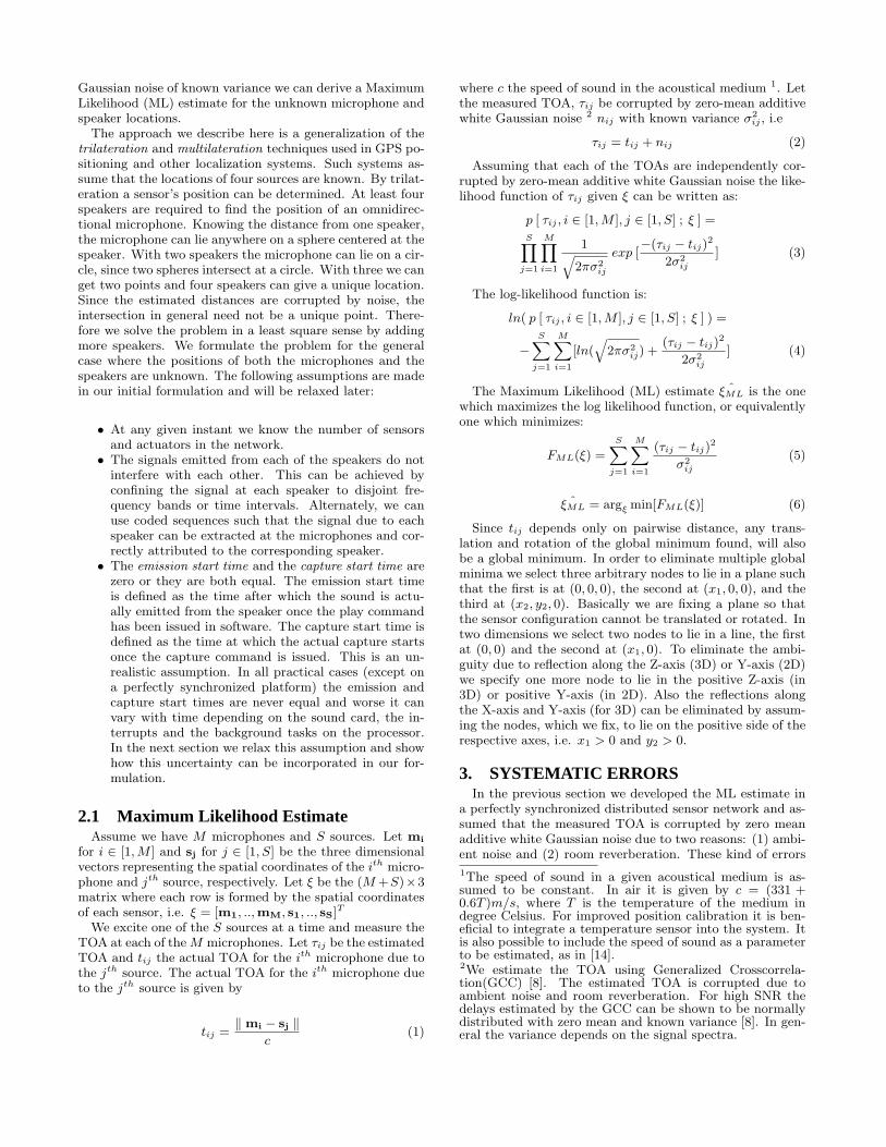
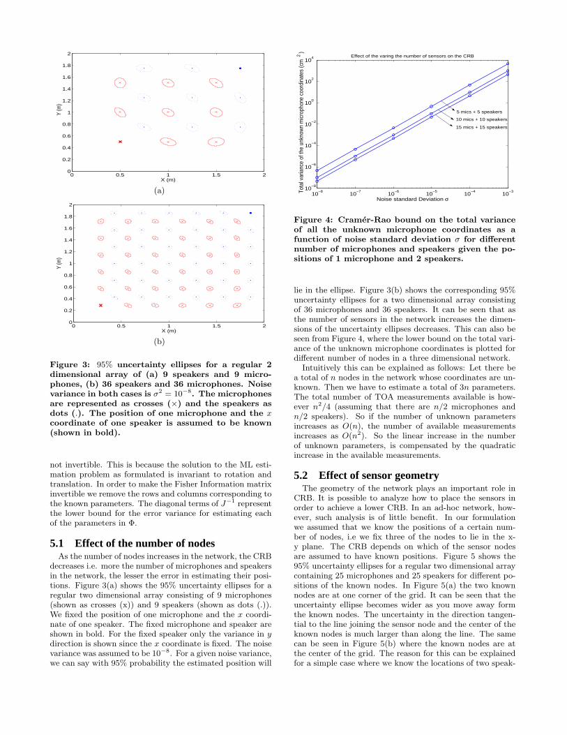
Figure 3: 95% uncertainty ellipses for a regular 2dimensional array of (a) 9 speakers and 9 micro-phones, (b) 36 speakers and 36 microphones. Noisevariance in both cases is σ2 = 10−8. The microphonesare represented as crosses (×) and the speakers asdots (.). The position of one microphone and the xcoordinate of one speaker is assumed to be known(shown in bold).
not invertible. This is because the solution to the ML esti-mation problem as formulated is invariant to rotation andtranslation. In order to make the Fisher Information matrixinvertible we remove the rows and columns corresponding tothe known parameters. The diagonal terms of J−1 representthe lower bound for the error variance for estimating eachof the parameters in Φ.
5.1 Effect of the number of nodesAs the number of nodes increases in the network, the CRB
decreases i.e. more the number of microphones and speakersin the network, the lesser the error in estimating their posi-tions. Figure 3(a) shows the 95% uncertainty ellipses for aregular two dimensional array consisting of 9 microphones(shown as crosses (x)) and 9 speakers (shown as dots (.)).We fixed the position of one microphone and the x coordi-nate of one speaker. The fixed microphone and speaker areshown in bold. For the fixed speaker only the variance in ydirection is shown since the x coordinate is fixed. The noisevariance was assumed to be 10−8. For a given noise variance,we can say with 95% probability the estimated position will
10−8
10−7
10−6
10−5
10−4
10−3
10−8
10−6
10−4
10−2
100
102
104
Noise standard Deviation σ
Tota
l var
ianc
e of
the
unkn
own
mic
roph
one
coor
dina
tes
(cm
2
)
Effect of the varing the number of sensors on the CRB
5 mics + 5 speakers
10 mics + 10 speakers
15 mics + 15 speakers
Figure 4: Cramer-Rao bound on the total varianceof all the unknown microphone coordinates as afunction of noise standard deviation σ for differentnumber of microphones and speakers given the po-sitions of 1 microphone and 2 speakers.
lie in the ellipse. Figure 3(b) shows the corresponding 95%uncertainty ellipses for a two dimensional array consistingof 36 microphones and 36 speakers. It can be seen that asthe number of sensors in the network increases the dimen-sions of the uncertainty ellipses decreases. This can also beseen from Figure 4, where the lower bound on the total vari-ance of the unknown microphone coordinates is plotted fordifferent number of nodes in a three dimensional network.
Intuitively this can be explained as follows: Let there bea total of n nodes in the network whose coordinates are un-known. Then we have to estimate a total of 3n parameters.The total number of TOA measurements available is how-ever n2/4 (assuming that there are n/2 microphones andn/2 speakers). So if the number of unknown parametersincreases as O(n), the number of available measurementsincreases as O(n2). So the linear increase in the numberof unknown parameters, is compensated by the quadraticincrease in the available measurements.
5.2 Effect of sensor geometryThe geometry of the network plays an important role in
CRB. It is possible to analyze how to place the sensors inorder to achieve a lower CRB. In an ad-hoc network, how-ever, such analysis is of little benefit. In our formulationwe assumed that we know the positions of a certain num-ber of nodes, i.e we fix three of the nodes to lie in the x-y plane. The CRB depends on which of the sensor nodesare assumed to have known positions. Figure 5 shows the95% uncertainty ellipses for a regular two dimensional arraycontaining 25 microphones and 25 speakers for different po-sitions of the known nodes. In Figure 5(a) the two knownnodes are at one corner of the grid. It can be seen that theuncertainty ellipse becomes wider as you move away formthe known nodes. The uncertainty in the direction tangen-tial to the line joining the sensor node and the center of theknown nodes is much larger than along the line. The samecan be seen in Figure 5(b) where the known nodes are atthe center of the grid. The reason for this can be explainedfor a simple case where we know the locations of two speak-

0 0.5 1 1.5 20
0.2
0.4
0.6
0.8
1
1.2
1.4
1.6
1.8
2
X (m)
Y (
m)
(a)
0 0.5 1 1.5 20
0.2
0.4
0.6
0.8
1
1.2
1.4
1.6
1.8
2
X (m)
Y (
m)
(b)
0 0.5 1 1.5 20
0.2
0.4
0.6
0.8
1
1.2
1.4
1.6
1.8
2
X (m)
Y (
m)
(c) (d)
Figure 5: 95% uncertainty ellipses for a regular 2 dimensional array of 25 microphones shown in solid linesand 25 speakers shown in dotted lines for different positions of the known microphone and for different xcoordinates of the known speaker. In (a) and (b) the known nodes are close to each other and in (c) they arespread out one at each corner of the grid. The microphones are represented as crosses (×) and the speakersas dots (.). Noise variance in all cases was σ2 = 10−9. (d) Schematic to explain the shape of uncertaintyellipses
ers as shown in Figure 5(d). Each annulus represents theuncertainty in the distance estimation. The intersection ofthe two annuli corresponding to the two speakers gives theuncertainty region for the position of the sensor. As can beseen for nodes far away from the two speakers the regionwidens because of the decrease in the curvature. It is bene-ficial if the known nodes are on the edges of the network andas faraway from each other as possible. In Figure 5(c) theknown sensor nodes are on the edges of the network. As canbe seen there is a substantial reduction in the dimensions ofthe uncertainty ellipses.
6. MONTE CARLO SIMULATIONSWe performed a series of Monte Carlo simulations to com-
pare the experimental performance with the Cramer Raobound (CRB). Ten microphones and ten speakers were ran-domly selected in a room of dimensions 2.0m×2.0m×2.0m.Based on the geometry of the setup the actual TOA was cal-culated and then corrupted with zero mean additive whiteGaussian noise of variance σ2 in order to model the roomambient noise and reverberation. The TOA matrix wasgiven as an input to the Levenberg-Marquadrat minimiza-tion routine. The positions of two microphones and twospeakers were assumed to be known. The starting pointfor the minimization procedure was chosen to lie within asphere of 50cm for each of the nodes in the network. Foreach noise variance σ2, the results were averaged over 2000trials corresponding to different initial guesses.
Figure 6(a), shows the total variance of all the unknownmicrophone coordinates plotted against the noise standarddeviation σ. The corresponding CRB is also shown. It canbe seen that the experimental results match closely with thetheoretical bound. Figure 6(d) shows the average bias. Theestimator shows a slight bias. The bias could be due tothe particular optimization method used or due to the finitenumber of trials.
6.1 Random vs. intelligent initial guessThe common problem with minimization methods is that
they may get stuck in a local minimum. To avoid this weneed a very good initial guess of the locations. We regard
starting points within 50cm of the node’s true location as in-telligent initial guesses. Figure 6(b) shows the total varianceof the unknown microphone coordinates plotted against thenoise standard deviation σ for intelligent and random initialguess. Figure 6(e) shows the corresponding average bias. Itcan be seen that even though the bias is not that high, thevariance is substantially higher for the random case. Hencethe choice of initial configuration is very crucial.
6.2 Estimation of source emission timeWe also performed a series of simulations where the TOA
was assumed to be corrupted by the unknown source emis-sion times. Figure 6(c) and 6(f) show the total variance andaverage bias of the unknown microphone coordinates plottedagainst the source emission time with and without account-ing the source emission time in the ML estimation proce-dure. It can be seen that with the increase of unaccountedsource emission times, the bias and variance increase. How-ever, if the source emission times are estimated, too, thenthe bias becomes nearly zero and the variance is also muchlower.
7. SYSTEM DESIGN ISSUESIn this section we discuss some of the practical issues of
our real-time implementation such as the type of calibrationsignal and the TOA estimation procedure used as well asother design choices.
7.1 Calibration signalsIn order to measure the TOA accurately the calibration
signal has to be appropriately selected and the parametersproperly tuned. Chirp signals and Maximum Likelihood(ML) sequences are the two most popular sequences used.A linear chirp signal is a short pulse in which the frequencyof the signal varies linearly between two preset frequencies.The cosine linear chirp signal of duration T with the in-stantaneous frequency varying linearly between f0 and f1 isgiven by
s(t) = Acos(2π(f0 + (f1 − f0
T)t)) 0 ≤ t ≤ T (26)

10−7
10−6
10−5
10−4
10−3
10−6
10−4
10−2
100
102
104
Noise Standard Deviation σ
To
tal v
aria
nce
of th
e e
rro
r in
th
e m
icro
ph
on
e c
oo
rdin
ate
s (
cm 2 )
Cramer Rao BoundEstimated over 2000 trials
(a)
10−7
10−6
10−5
10−4
10−3
10−6
10−4
10−2
100
102
Noise Standard Deviation σ
To
tal v
aria
nce
of
the
err
or
in t
he
mic
rop
ho
ne
co
ord
ina
tes
( cm
2
)
Random GuessIntelligent Guess
(b)
0 200 400 600 800 100010
−12
10−10
10−8
10−6
10−4
10−2
100
102
104
Unknown Source Emission Time (microseconds)
To
tal v
aria
nce
of th
e e
rro
r in
th
e m
icro
ph
on
e c
oo
rdin
ate
s (
cm
2)
Without source emission time estimationWith source emission time estimation
(c)
10−7
10−6
10−5
10−4
10−3
−0.05
0
0.05
0.1
0.15
0.2
0.25
0.3
0.35
0.4
0.45
Noise Standard Deviation σ
Ave
rag
e B
ias o
f th
e e
rro
r (c
m)
(d)
10−7
10−6
10−5
10−4
10−3
−5
−4
−3
−2
−1
0
1
Noise Standard Deviation σ
Ave
rag
e B
ias
of th
e e
rro
r (c
m)
Intelligent GuessRandom Guess
(e)
0 200 400 600 800 1000−8
−7
−6
−5
−4
−3
−2
−1
0
1
Unknown Source Emission time (microseconds)
Ave
rag
e B
ias
of th
e e
rro
r (c
m)
Without source emission time estimationWith source emission time estimation
(f)
Figure 6: Monte Carlo Simulation results: (a) (b) and (c) Total variance of the error in all the unknownmicrophone coordinates and (d)(e) and (f) average bias of the error for a network consisting of 10 microphonesand 10 speakers. The positions of 2 microphones and 2 speakers are assumed to be known.
In our system, we used the chirp signal of 512 samples at44.1kHz (11.61 ms) as our calibration signal. The instanta-neous frequency varied linearly from 5 kHz to 10 kHz. Theinitial and the final frequency was chosen to lie in the com-mon passband of the microphone and the speaker frequencyresponse. The chirp signal send by the speaker is convolvedwith the room impulse response resulting in the spreading ofthe chirp signal. Figure 7(a) shows the chirp signal as sentout by the soundcard to the speaker. This signal is recordedby looping the output channel directly back to an inputchannel, on a multichannel sound card. The initial delay isdue to the emission start time and the capture start time.Figure 7(b) shows the corresponding chirp signal receivedby the microphone. The chirp signal is delayed by a certainamount due to the propagation path. The distortion andthe spreadout is due to the speaker, microphone and roomresponse. Figure 7(c) and Figure 7(d) show the magnitudeof the frequency response of the transmitted chirp signal andthe received chirp signal, respectively.
One of the problems in accurately estimating the TOAis due to the multipath propagation caused by room reflec-tions. This can be seen in the received chirp signal where theinitial part corresponds to the direct signal and the rest arethe room reflections. We use the Time Division Multiplexingscheme to send the calibration signal to different speakers.To avoid interference between the different calibration sig-
nals we zeropad the calibration signal appropriately in de-pendence of the room reverberation level and the maximumdelay. Alternatively, we could also use Frequency DivisionMultiplexing by allocating a frequency band at each chan-nel or spread spectrum techniques by using different MLsequences for each channel. The advantage would be thatall the output channels can be played simultaneously. How-ever extra processing is needed at the input to separate thesignals.
7.2 TOA estimationThis is the most crucial part of the algorithm and also a
potential source of error. Hence lot of care has to be takento get the TOA accurately in noisy and reverberant environ-ments. The time-delay may be found by locating the peak inthe cross-correlation of the signals received over the two mi-crophones. However this method is not robust to noise andreverberations. Knapp and Carter [8] developed a MaximumLikelihood (ML) estimator for determining the time delaybetween signals received at two spatially separated sensorsin the presence of uncorrelated noise. In this method, thedelay estimate is the time lag which maximizes the cross-correlation between filtered versions of the received signals[8]. The cross-correlation of the filtered versions of the sig-nals is called as the Generalized Cross Correlation (GCC)function. The GCC function Rx1x2(τ) is computed as [8]

0 20 40 60 80−1
−0.5
0
0.5
1
Time (ms)
Refer
ence
chirp
sign
al
0 20 40 60 80
−0.2
−0.1
0
0.1
0.2
0.3
Time (ms)
Rece
ived c
hirp s
ignal
0 5 10 15 20−40
−20
0
20
40
Frequency (kHz)
dB
0 5 10 15 20−40
−20
0
20
40
Frequency (kHz)
dB
(a) (b)
(c) (d)
Figure 7: (a) The loopback reference chirp signal (b)the chirp signal received by one of the microphones(c) the magnitude of the frequency response of thereference signal and (d) the received chirp signal
Rx1x2(τ) =∫∞−∞W (ω)X1(ω)X∗2 (ω)ejωτdω, where X1(ω),
X2(ω) are the Fourier transforms of the microphone signalsx1(t), x2(t), respectively and W (ω) is the weighting func-tion. The two most commonly using weighting functionsare the ML and the Phase Transform (PHAT) weighting.The ML weighting function, accentuates the signal passedto the correlator at frequencies for which the signal-to-noiseratio is the highest and, simultaneously suppresses the noisepower [8]. This ML weighting function performs well for lowroom reverberation. As the room reverberation increasesthis method shows severe performance degradations. Sincethe spectral characteristics of the received signal are modi-fied by the multipath propagation in a room, the GCC func-tion is made more robust by deemphasizing the frequencydependent weightings. The Phase Transform is one extremewhere the magnitude spectrum is flattened. The PHATweighting is given by WPHAT (ω) = 1
|X1(ω)X∗2 (ω)| . By flat-
tening out the magnitude spectrum the resulting peak in theGCC function corresponds to the dominant delay. However,the disadvantage of the PHAT weighting is that it placesequal emphasizes on both the low and high SNR regions,and hence it works well only when the noise level is low.For low noise rooms the PHAT method performs moder-ately well. For a practical room we can estimate the roomnoise, and use the combined ML and PHAT weighting byappropriately emphasizing each weighting function based onthe noise levels [6]. A more accurate estimate of the peakcan be found by upsampling the GCC function.
7.3 Testbed SetupThe real-time setup has been tested in a synchronized as
well as a distributed setup using laptops. Figure 8 shows thetop view of our experimental setup. Four omnidirectionalmicrophones (RadioShack) and four loudspeakers (MackieHR624) were setup in a room with low reverberation andlow ambient noise. The ground truth was measured man-ually to validate the results from the position calibrationmethods. In a synchronized setup, the microphones andloudspeakers were interfaced using an RME DIGI9652 card.For a distributed implementation the loudspeakers and themicrophones were connected to four laptops (3 IBM T-seriesThinkpads and one Dell laptop). All the laptops had IntelPentium series processors.
����
����
����
����
��� ��
��� ��
��� ��
��� ��
�
�
���������� �������
����
�������
�������
����
�������
�������
Figure 8: Top view of the whisper room containing4 microphones and 4 speakers
����������������� ���������������
�� ���� ���������������������� �����
�����������������������
����������� ����� ����
��������� �����!�����������!
��������������"���� ���������
#$%��� ������
#$%
#$%������&
����������������
���'������������
��"���
���'��(���)�����
Figure 9: Schematic showing the distributed controlscheme.
7.4 Software detailsCapture and play back was done using the free, cross plat-
form, open-source, audio I/O library Portaudio [3]. Mostof the signal processing tasks were implemented using theSignal Processing Library in Intelr Integrated PerformancePrimitives (IPP). IPP is a cross-platform low-level softwarelayer that abstracts multimedia functionality from the pro-cessor underneath providing highly optimized code [2]. Forthe non-linear minimization we used the mrqmin routinefrom Numerical Recipes in C [12]. For displaying the cali-brated microphones and speakers we used the OpenGL Util-ity Toolkit (GLUT) ported to Win32 [4].
For the distributed platform we used the UPnP [1] tech-nology to form an adhoc network and control the audiodevices on different platforms. UPnP technology is a dis-tributed, open networking architecture that employs TCP/IPand other Internet technologies to enable seamless proxim-ity networking [1]. The real time setup integrates the dis-tributed synchronization scheme using ML sequence as pro-posed in [10]. Figure 9 shows a schematic of the TOAcomputation protocol. Each of the laptops has an UPnPservice running for playing the chirp signal and capturingthe audio stream. One of the GPC’s is configured to be themaster which plays the ML sequence as described in [10]. A

Figure 10: A sample screen shot of the OpenGLdisplay.
program on the master scans the network for all the avail-able UPnP players. Then the chirp signal is played on eachof the devices one after the other and the signal is captured.The TOA computation is distributed among all the laptops,in that each laptop computes its own TOA and reports itback to the master. The master performs the minimizationroutine once it has the TOA matrix.
As regards to CPU utilization the TOA estimation con-sumes negligible resources. If we use a good initial guess viathe Multidimensional Scaling technique then the minimiza-tion routine converges within 8 to 10 iterations.
7.5 ResultsFor the setup consisting of 4 speakers and 4 microphones,
the sensors’ and actuators’ three dimensional locations couldbe estimated with an average bias of 0.08 cm and averagestandard deviation of 3.8 cm (results averaged over 100 tri-als). In order to display the microphones and speakers incontext of the room, the positions of two speakers and onemicrophone was assumed to be known. Figure 10 showsa snapshot of the OpenGL display, showing the estimatedlocations of the speakers and microphones.
8. SUMMARY AND FURTHER STUDIESIn this paper we described the problem of localization of
acoustic sensors and actuators in a network of distributedgeneral-purpose computing platforms. Our approach allowsputting laptops, PDAs and tablets into a common 3D co-ordinate system. Together with time synchronization thiscreates arrays of audio sensors and actuators and enablesa rich set of new multistream A/V applications on plat-forms that available virtually anywhere. We also derivedimportant bounds on performance of spatial localization al-gorithms, proposed optimization techniques to implementthem and extensively validated the algorithms on simulatedand real data. There are a number of ways to improve lo-calization in the future. The one we are currently pursuingis targeted at using Time Difference Of Arrival instead ofTime Of Arrival and getting closed form approximations tobe used as initial guess for the minimization routine.
9. ACKNOWLEDGMENTSThe authors would like to acknowledge the help of Dr.
Bob Liang, Dr.Amit Roy Chowdhury and Dr.Ramani Du-raiswami who contributed valuable comments and sugges-tions for this work. We would also like to thank the threeanonymous reviewers and our shepherd Dr.Dongyan Xu forthe reviews and comments which helped to improve the over-all quality of the paper.
10. REFERENCES[1] http://intel.com/technology/upnp/.
[2] http://www.intel.com/software/products/perflib/.
[3] http://www.portaudio.com/.
[4] http://www.xmission.com/nate/glut.html.
[5] D. P. Betrsekas. Nonlinear Programming. AthenaScientific, 1995.
[6] M. Brandstein, J. Adcock, and H. Silverman. Apractical time-delay estimator for localizing speechsources with a microphone array. Comput. SpeechLang., 9:153–169, September 1995.
[7] L. Girod, V. Bychkovskiy, J. Elson, and D. Estrin.Locating tiny sensors in time and space: A case study.In Proc. International Conference on ComputerDesign, September 2002.
[8] C. H. Knapp and G. C. Carter. The generalizedcorrelation method for estimation of time delay. IEEETrans. Acoust., Speech, Signal Processing,ASSP-24(4):320–327, August 1976.
[9] A. M. Ladd, K. E. Bekris, A. Rudys, G. Marceau,L. E. Kavraki, and D. S. Wallach. Robotics-basedlocation sensing using wireless Ethernet. InProceedings of The Eighth ACM InternationalConference on Mobile Computing and Networking(MOBICOM), Atlanta, GA, USA, Sept. 2002.
[10] R. Lienhart, I. Kozintsev, S. Wehr, and M. Yeung. Onthe importance of exact synchronization fordistributed audio processing. In Proc. IEEE Int. Conf.Acoust., Speech, Signal Processing, April 2003.
[11] R. Moses, D. Krishnamurthy, and R. Patterson. Aself-localization method for wireless sensor networks.Eurasip Journal on Applied Signal Processing SpecialIssue on Sensor Networks, 2003(4):348–358, March2003.
[12] H. P. Press, S. A. Teukolsky, W. T. Vettring, andB. P. Flannery. Numerical Recipes in C The Art ofScientific Computing. Cambridge University Press, 2edition, 1995.
[13] Y. Rockah and P. M. Schultheiss. Array shapecalibration using sources in unknown locations PartII: Near-field sources and estimator implementation.IEEE Trans. Acoust., Speech, Signal Processing,ASSP-35(6):724–735, June 1987.
[14] J. M. Sachar, H. F. Silverman, and W. R.Patterson III. Position calibration of large-aperturemicrophone arrays. In Proc. IEEE Int. Conf. Acoust.,Speech, Signal Processing, pages II–1797 – II–1800,2002.
[15] A. Savvides, C. C. Han, and M. B. Srivastava.Dynamic fine-grained localization in ad-hoc wirelesssensor networks. In Proc. International Conference onMobile Computing and Networking, July 2001.
[16] W. S. Torgerson. Multidimensional scaling: I. theoryand method. Psychometrika, 17:401–419, 1952.
[17] H. L. Van Trees. Detection, Estimation, andModulation Theory, volume Part 1.Wiley-Interscience, 2001.
[18] A. J. Weiss and B. Friedlander. Array shapecalibration using sources in unknown locations-amaxilmum-likelihood approach. IEEE Trans. Acoust.,Speech, Signal Processing, 37(12):1958–1966,December 1989.