Positive Semidefinite Metric Learning Using Boosting-like Algorithms

Journal of Machine Learning Research 13 (2012) 1007-1036 Submitted 2/11; Revised 1/12; Published 4/12

Positive Semidefinite Metric Learning Using Boosting-like Algorithms

Chunhua Shen CHUNHUA.SHEN@ADELAIDE .EDU.AU

The University of AdelaideAdelaide, SA 5005, Australia

Junae Kim JUNAE.KIM @NICTA .COM.AU

NICTA, Canberra Research LaboratoryLocked Bag 8001Canberra, ACT 2601, Australia

Lei Wang [email protected]

University of WollongongWollongong, NSW 2522, Australia

Anton van den Hengel ANTON.VANDENHENGEL@ADELAIDE .EDU.AU

The University of AdelaideAdelaide, SA 5005, Australia

Editors: Soren Sonnenburg, Francis Bach, Cheng Soon Ong

Abstract

The success of many machine learning and pattern recognition methods relies heavily upon theidentification of an appropriate distance metric on the input data. It is often beneficial to learn such ametric from the input training data, instead of using a default one such as the Euclidean distance. Inthis work, we propose a boosting-based technique, termed BOOSTMETRIC, for learning a quadraticMahalanobis distance metric. Learning a valid Mahalanobisdistance metric requires enforcingthe constraint that the matrix parameter to the metric remains positive semidefinite. Semidefiniteprogramming is often used to enforce this constraint, but does not scale well and is not easy toimplement. BOOSTMETRIC is instead based on the observation that any positive semidefinite ma-trix can be decomposed into a linear combination of trace-one rank-one matrices. BOOSTMETRIC

thus uses rank-one positive semidefinite matrices as weak learners within an efficient and scalableboosting-based learning process. The resulting methods are easy to implement, efficient, and canaccommodate various types of constraints. We extend traditional boosting algorithms in that itsweak learner is a positive semidefinite matrix with trace andrank being one rather than a classifieror regressor. Experiments on various data sets demonstratethat the proposed algorithms comparefavorably to those state-of-the-art methods in terms of classification accuracy and running time.

Keywords: Mahalanobis distance, semidefinite programming, column generation, boosting, La-grange duality, large margin nearest neighbor

1. Introduction

The identification of an effective metric by which to measure distances between data points is anessential component of many machine learning algorithms includingk-nearest neighbor (kNN), k-means clustering, and kernel regression. These methods have been applied to a range of problems,including image classification and retrieval (Hastie and Tibshirani, 1996; Yuet al., 2008; Jian and

c©2012 Chunhua Shen, Junae Kim, Lei Wang and Anton van den Hengel.

SHEN, K IM , WANG AND VAN DEN HENGEL

Vemuri, 2007; Xing et al., 2002; Bar-Hillel et al., 2005; Boiman et al., 2008;Frome et al., 2007)amongst a host of others.

The Euclidean distance has been shown to be effective in a wide variety ofcircumstances.Boiman et al. (2008), for instance, showed that in generic object recognition with local features,kNN with a Euclidean metric can achieve comparable or better accuracy than more sophisticatedclassifiers such as support vector machines (SVMs). The Mahalanobisdistance represents a gen-eralization of the Euclidean distance, and offers the opportunity to learn a distance metric directlyfrom the data. This learned Mahalanobis distance approach has been shown to offer improved per-formance over Euclidean distance-based approaches, and was particularly shown by Wang et al.(2010b) to represent an improvement upon the method of Boiman et al. (2008). It is the prospectof a significant performance improvement from fundamental machine learning algorithms whichinspires the approach presented here.

If we let ai , i = 1,2· · · , represent a set of points inRD, then the Mahalanobis distance, orGaussian quadratic distance, between two points is

‖ai −a j‖X =√

(ai −a j)⊤X(ai −a j),

whereX < 0 is a positive semidefinite (p.s.d.) matrix. The Mahalanobis distance is thus param-eterized by a p.s.d. matrix, and methods for learning Mahalanobis distances are therefore oftenframed as constrained semidefinite programs. The approach we proposehere, however, is basedon boosting, which is more typically used for learning classifiers. The primary motivation for theboosting-based approach is that it scales well, but its efficiency in dealingwith large data sets is alsoadvantageous. The learning of Mahalanobis distance metrics representsa specific application of amore general method for matrix learning which we present below.

We are interested here in the case where the training data consist of a set of constraints upon therelative distances between data points,

I = {(ai ,a j ,ak) |disti j < distik}, (1)

wheredisti j measures the distance betweenai and a j . Each such constraint implies that “ai iscloser toa j thanai is to ak”. Constraints such as these often arise when it is known thatai anda j

belong to the same class of data points whileai ,ak belong to different classes. These comparisonconstraints are thus often much easier to obtain than either the class labels or distances between dataelements (Schultz and Joachims, 2003). For example, in video content retrieval, faces extracted fromsuccessive frames at close locations can be safely assumed to belong to the same person, withoutrequiring the individual to be identified. In web search, the results returned by a search engineare ranked according to the relevance, an ordering which allows a natural conversion into a set ofconstraints.

The problem of learning a p.s.d. matrix such asX can be formulated in terms of estimating aprojection matrixL whereX = LL⊤. This approach has the advantage that the p.s.d. constraintis enforced through the parameterization, but the disadvantage is that the relationship between thedistance measure and the parameter matrix is less direct. In practice this approach has lead to local,rather than globally optimal solutions, however (see Goldberger et al., 2004 for example).

Methods such as Xing et al. (2002), Weinberger et al. (2005), Weinberger and Saul (2006) andGloberson and Roweis (2005) which seekX directly are able to guarantee global optimality, butat the cost of a heavy computational burden and poor scalability as it is nottrivial to preserve the

1008

METRIC LEARNING USING BOOSTING-LIKE ALGORITHMS

semidefiniteness ofX during the course of learning. Standard approaches such as interior-point (IP)Newton methods need to calculate the Hessian. This typically requiresO(D4) storage and has worst-case computational complexity of approximatelyO(D6.5) whereD is the size of the p.s.d. matrix.This is prohibitive for many real-world problems. An alternating projected (sub-)gradient approachis adopted in Weinberger et al. (2005), Xing et al. (2002) and Globerson and Roweis (2005). Thedisadvantages of this algorithm, however, are: 1) it is not easy to implement; 2) many parametersare involved; 3) usually it converges slowly.

We propose here a method for learning a p.s.d. matrix labeled BOOSTMETRIC. The methodis based on the observation that any positive semidefinite matrix can be decomposed into a lin-ear positive combination of trace-one rank-one matrices. The weak learner in BOOSTMETRIC isthus a trace-one rank-one p.s.d. matrix. The proposed BOOSTMETRIC algorithm has the followingdesirable properties:

1. BOOSTMETRIC is efficient and scalable. Unlike most existing methods, no semidefinite pro-gramming is required. At each iteration, only the largest eigenvalue and its correspondingeigenvector are needed.

2. BOOSTMETRIC can accommodate various types of constraints. We demonstrate the use ofthe method to learn a Mahalanobis distance on the basis of a set of proximity comparisonconstraints.

3. Like AdaBoost, BOOSTMETRIC does not have any parameter to tune. The user only needs toknow when to stop. Also like AdaBoost it is easy to implement. No sophisticated optimiza-tion techniques are involved. The efficacy and efficiency of the proposed BOOSTMETRIC isdemonstrated on various data sets.

4. We also propose a totally-corrective version of BOOSTMETRIC. As in TotalBoost (Warmuthet al., 2006) the weights of all the selected weak learners (rank-one matrices) are updated ateach iteration.

Both the stage-wise BOOSTMETRIC and totally-corrective BOOSTMETRIC methods are veryeasy to implement.

The primary contributions of this work are therefore as follows: 1) We extend traditional boost-ing algorithms such that each weak learner is a matrix with the trace and rank ofone—which mustbe positive semidefinite—rather than a classifier or regressor; 2) The proposed algorithm can beused to solve many semidefinite optimization problems in machine learning and computer vision.We demonstrate the scalability and effectiveness of our algorithms on metric learning. Part of thiswork appeared in Shen et al. (2008, 2009). More theoretical analysisand experiments are includedin this version. Next, we review some relevant work before we present our algorithms.

1.1 Related Work

Distance metric learning is closely related to subspace methods. Principal component analysis(PCA) and linear discriminant analysis (LDA) are two classical dimensionality reduction tech-niques. PCA finds the subspace that captures the maximum variance within theinput data whileLDA tries to identify the projection which maximizes the between-class distance and minimizes thewithin-class variance. Locality preserving projection (LPP) finds a linearprojection that preserves

1009


the neighborhood structure of the data set (He et al., 2005). Essentially,LPP linearly approximatesthe eigenfunctions of the Laplace Beltrami operator on the underlying manifold. The connectionbetween LPP and LDA is also revealed in He et al. (2005). Wang et al. (2010a) extended LPP tosupervised multi-label classification. Relevant component analysis (RCA)(Bar-Hillel et al., 2005)learns a metric fromequivalenceconstraints. RCA can be viewed as extending LDA by incorpo-rating must-link constraints and cannot-link constraints into the learning procedure. Each of thesemethods may be seen as devising a linear projection from the input space to a lower-dimensionaloutput space. If this projection is characterized by the matrixL , then note that these methods maybe related to the problem of interest here by observingX = LL⊤. This typically implies thatX isrank-deficient.

Recently, there has been significant research interest in supervised distance metric learning usingside information that is typically presented in a set of pairwise constraints. Most of these methods,although appearing in different formats, share a similar essential idea: to learn an optimal dis-tance metric by keeping training examples in equivalence constraints close, and at the same time,examples in in-equivalence constraints well separated. Previous work of Xing et al. (2002), Wein-berger et al. (2005), Jian and Vemuri (2007), Goldberger et al. (2004), Bar-Hillel et al. (2005) andSchultz and Joachims (2003) fall into this category. The requirement thatX must be p.s.d. has ledto the development of a number of methods for learning a Mahalanobis distance which rely uponconstrained semidefinite programing. This approach has a number of limitations, however, whichwe now discuss with reference to the problem of learning a p.s.d. matrix froma set of constraintsupon pairwise-distance comparisons. Relevant work on this topic includesBar-Hillel et al. (2005),Xing et al. (2002), Jian and Vemuri (2007), Goldberger et al. (2004), Weinberger et al. (2005) andGloberson and Roweis (2005) amongst others.

Xing et al. (2002) first proposed the idea of learning a Mahalanobis metricfor clustering usingconvex optimization. The inputs are two sets: a similarity set and a dis-similarity set.The algorithmmaximizes the distance between points in the dis-similarity set under the constraintthat the distancebetween points in the similarity set is upper-bounded. Neighborhood component analysis (NCA)(Goldberger et al., 2004) and large margin nearest neighbor (LMNN) (Weinberger et al., 2005)learn a metric by maintaining consistency in data’s neighborhood and keep a large margin at theboundaries of different classes. It has been shown in Weinberger and Saul (2009); Weinberger et al.(2005) that LMNN delivers the state-of-the-art performance among most distance metric learningalgorithms. Information theoretic metric learning (ITML) learns a suitable metric based on infor-mation theoretics (Davis et al., 2007). To partially alleviate the heavy computationof standard IPNewton methods, Bregman’s cyclic projection is used in Davis et al. (2007).This idea is extendedin Wang and Jin (2009), which has a closed-form solution and is computationally efficient.

There have been a number of approaches developed which aim to improvethe scalability ofthe process of learning a metric parameterized by a p.s.d. metricX. For example, Rosales and Fung(2006) approximate the p.s.d. cone using a set of linear constraints basedon the diagonal dominancetheorem. The approximation is not accurate, however, in the sense that it imposes too strong a con-dition on the learned matrix—one may not want to learn a diagonally dominant matrix. Alternativeoptimization is used in Xing et al. (2002) and Weinberger et al. (2005) to solve the semidefiniteproblem iteratively. At each iteration, a full eigen-decomposition is applied toproject the solu-tion back onto the p.s.d. cone. BOOSTMETRIC is conceptually very different to this approach, andadditionally only requires the calculation of the first eigenvector. Tsuda etal. (2005) proposed touse matrix logarithms and exponentials to preserve positive definiteness. For the application of

1010


semidefinite kernel learning, they designed a matrix exponentiated gradientmethod to optimize vonNeumann divergence based objective functions. At each iteration of matrix exponentiated gradient,a full eigen-decomposition is needed. In contrast, we only need to find the leading eigenvector.

The approach proposed here is directly inspired by the LMNN proposedin Weinberger and Saul(2009); Weinberger et al. (2005). Instead of using the hinge loss, however, we use the exponentialloss and logistic loss functions in order to derive an AdaBoost-like (or LogitBoost-like) optimizationprocedure. In theory, any differentiable convex loss function can beapplied here. Hence, despitesimilar purposes, our algorithm differs essentially in the optimization. While the formulation ofLMNN looks more similar to SVMs, our algorithm, termed BOOSTMETRIC, largely draws uponAdaBoost (Schapire, 1999).

Column generation was first proposed by Dantzig and Wolfe (1960) for solving a particularform of structured linear program with an extremely large number of variables. The general ideaof column generation is that, instead of solving the original large-scale problem (master problem),one works on a restricted master problem with a reasonably small subset ofthe variables at eachstep. The dual of the restricted master problem is solved by the simplex method,and the optimaldual solution is used to find the new column to be included into the restricted masterproblem. LP-Boost (Demiriz et al., 2002) is a direct application of column generation in boosting. Significantly,LPBoost showed that in an LP framework, unknown weak hypotheses can be learned from the dualalthough the space of all weak hypotheses is infinitely large. Shen and Li (2010) applied columngeneration to boosting with general loss functions. It is these results that underpin BOOSTMETRIC.

The remaining content is organized as follows. In Section 2 we present some preliminary math-ematics. In Section 3, we show the main results. Experimental results are provided in Section4.

2. Preliminaries

We introduce some fundamental concepts that are necessary for setting up our problem. First, thenotation used in this paper is as follows.

2.1 Notation

Throughout this paper, a matrix is denoted by a bold upper-case letter (X); a column vector isdenoted by a bold lower-case letter (xxx). The ith row of X is denoted byX i: and theith columnX:i .111 and 000 are column vectors of 1’s and 0’s, respectively. Their size should beclear from the context.We denote the space ofD×D symmetric matrices bySD, and positive semidefinite matrices bySD

+.Tr (·) is the trace of a symmetric matrix and〈X,Z〉 = Tr (XZ⊤) = ∑i j X i j Z i j calculates the innerproduct of two matrices. An element-wise inequality between two vectors likeuuu≤ vvv meansui ≤ vi

for all i. We useX < 0 to indicate that matrixX is positive semidefinite. For a matrixX ∈ SD, the

following statements are equivalent: 1)X < 0 (X ∈ SD+); 2) All eigenvalues ofX are nonnegative

(λi(X)≥ 0, i = 1, · · · ,D); and 3)∀uuu∈ RD, uuu⊤Xuuu≥ 0.

2.2 A Theorem on Trace-one Semidefinite Matrices

Before we present our main results, we introduce an important theorem that serves the theoreticalbasis of BOOSTMETRIC.

1011


Definition 1 For any positive integer m, given a set of points{xxx1, ...,xxxm} in a real vector or matrixspaceSp, theconvex hullof Spspanned by m elements inSp is defined as:

Convm(Sp) ={

∑mi=1wixxxi

∣∣∣wi ≥ 0,∑m

i=1wi = 1,xxxi ∈ Sp}

.

Define the linear convex span ofSpas:1

Conv(Sp) =⋃

m

Convm(Sp) ={

∑mi=1wixxxi

∣∣∣wi ≥ 0,∑m

i=1wi = 1,xxxi ∈ Sp,m∈ Z+

}

.

HereZ+ denotes the set of all positive integers.

Definition 2 Let us defineΓ1 to be the space of all positive semidefinite matricesX ∈ SD+ with trace

equaling one:Γ1 = {X |X < 0,Tr (X) = 1} ;

andΨ1 to be the space of all positive semidefinite matrices with both trace and rank equaling one:

Ψ1 = {Z |Z < 0,Tr (Z) = 1,Rank(Z) = 1} .

We also defineΓ2 as the convex hull ofΨ1, that is,

Γ2 = Conv(Ψ1).

Lemma 3 LetΨ2 be a convex polytope defined asΨ2 = {λλλ ∈RD|λk ≥ 0, ∀k= 0, · · · ,D, ∑D

k=1 λk =1}, then the points with only one element equaling one and all the others being zeros are the extremepoints (vertexes) ofΨ2. All the other points can not be extreme points.

Proof Without loss of generality, let us consider such a pointλλλ′ = {1,0, · · · ,0}. If λλλ′ is not anextreme point ofΨ2, then it must be possible to express it as a convex combination of a set ofother points in Ψ2: λλλ′ = ∑m

i=1wiλλλi , wi > 0, ∑mi=1wi = 1 andλλλi 6= λλλ′. Then we have equations:

∑mi=1wiλi

k = 0, ∀k = 2, · · · ,D. It follows thatλik = 0, ∀i andk = 2, · · · ,D. That means,λi

1 = 1 ∀i.This is inconsistent withλλλi 6= λλλ′. Therefore such a convex combination does not exist andλλλ′ mustbe an extreme point. It is trivial to see that anyλλλ that has more than one active element is an convexcombination of the above-defined extreme points. So they can not be extremepoints.

Theorem 4 Γ1 equals toΓ2; that is, Γ1 is also the convex hull ofΨ1. In other words, allZ ∈ Ψ1,form the set of extreme points ofΓ1.

Proof It is easy to check that any convex combination∑i wiZ i , such thatZ i ∈ Ψ1, resides inΓ1,with the following two facts: 1) a convex combination of p.s.d. matrices is still a p.s.d. matrix; 2)Tr

(

∑i wiZ i)= ∑iwi Tr (Z i) = 1.

By denotingλ1 ≥ ·· · ≥ λD ≥ 0 the eigenvalues of aZ ∈ Γ1, we know thatλ1 ≤ 1 because∑D

i=1 λi = Tr (Z) = 1. Therefore, all eigenvalues ofZ must satisfy:λi ∈ [0,1], ∀i = 1, · · · ,D and

1. With slight abuse of notation, we also use the symbolConv(·) to denote convex span. In general it is not a convexhull.

1012


∑Di λi = 1. By looking at the eigenvalues ofZ and using Lemma 3, it is immediate to see that a

matrixZ such thatZ < 0, Tr (Z) = 1 andRank(Z)> 1 can not be an extreme point ofΓ1. The onlycandidates for extreme points are those rank-one matrices (λ1 = 1 andλ2,··· ,D = 0). Moreover, it isnot possible that some rank-one matrices are extreme points and others arenot because the othertwo constraintsZ < 0 andTr (Z) = 1 do not distinguish between different rank-one matrices.

Hence, allZ ∈Ψ1 form the set of extreme points ofΓ1. Furthermore,Γ1 is a convex and compactset, which must have extreme points. The Krein-Milman Theorem (Krein and Milman, 1940) tellsus that a convex and compact set is equal to the convex hull of its extreme points.

This theorem is a special case of the results from Overton and Womersley (1992) in the contextof eigenvalue optimization. A different proof for the above theorem’s general version can also befound in Fillmore and Williams (1971).

In the context of semidefinite optimization, what is of interest about Theorem4 is as follows:it tells us that a bounded p.s.d. matrix constraintX ∈ Γ1 can be equivalently replaced with a set ofconstrains which belong toΓ2. At the first glance, this is a highly counterintuitive proposition be-causeΓ2 involves many more complicated constraints. Bothwi andZ i (∀i = 1, · · · ,m) are unknownvariables. Even worse,mcould be extremely (or even infinitely) large. Nevertheless, this is the typeof problems thatboostingalgorithms are designed to solve. Let us give a brief overview of boostingalgorithms.

2.3 Boosting

Boosting is an example of ensemble learning, where multiple learners are trained to solve the sameproblem. Typically a boosting algorithm (Schapire, 1999) creates a single strong learner by incre-mentally adding base (weak) learners to the final strong learner. The base learner has an importantimpact on the strong learner. In general, a boosting algorithm builds on a user-specified base learn-ing procedure and runs it repeatedly on modified data that are outputs from the previous iterations.

The general form of the boosting algorithm is sketched in Algorithm 1. The inputs to a boostingalgorithm are a set of training examplexxx, and their corresponding class labelsy. The final output isa strong classifier which takes the form

Fwww(xxx) = ∑Jj=1w jh j(xxx). (2)

Hereh j(·) is a base learner. From Theorem 4, we know that a matrixX ∈ Γ1 can be decomposed as

X = ∑Jj=1w jZ j ,Z j ∈ Γ2. (3)

By observing the similarity between Equations (2) and (3), we may viewZ j as a weak classifierand the matrixX as the strong classifier that we want to learn. This is exactly the problem thatboosting methods have been designed to solve. This observation inspires us to solve a special typeof semidefinite optimization problem using boosting techniques.

The sparse greedy approximation algorithm proposed by Zhang (2003)is an efficient method forsolving a class of convex problems, and achieves fast convergence rates. It has also been shown thatboosting algorithms can be interpreted within the general framework of Zhang (2003). The mainidea of sequential greedy approximation, therefore, is as follows. Given an initializationuuu0, whichis in a convex subset of a linear vector space, a matrix space or a functional space, the algorithmfindsuuui andλ ∈ (0,1) such that the objective functionF((1−λ)uuui−1+λuuui) is minimized. Then the

1013


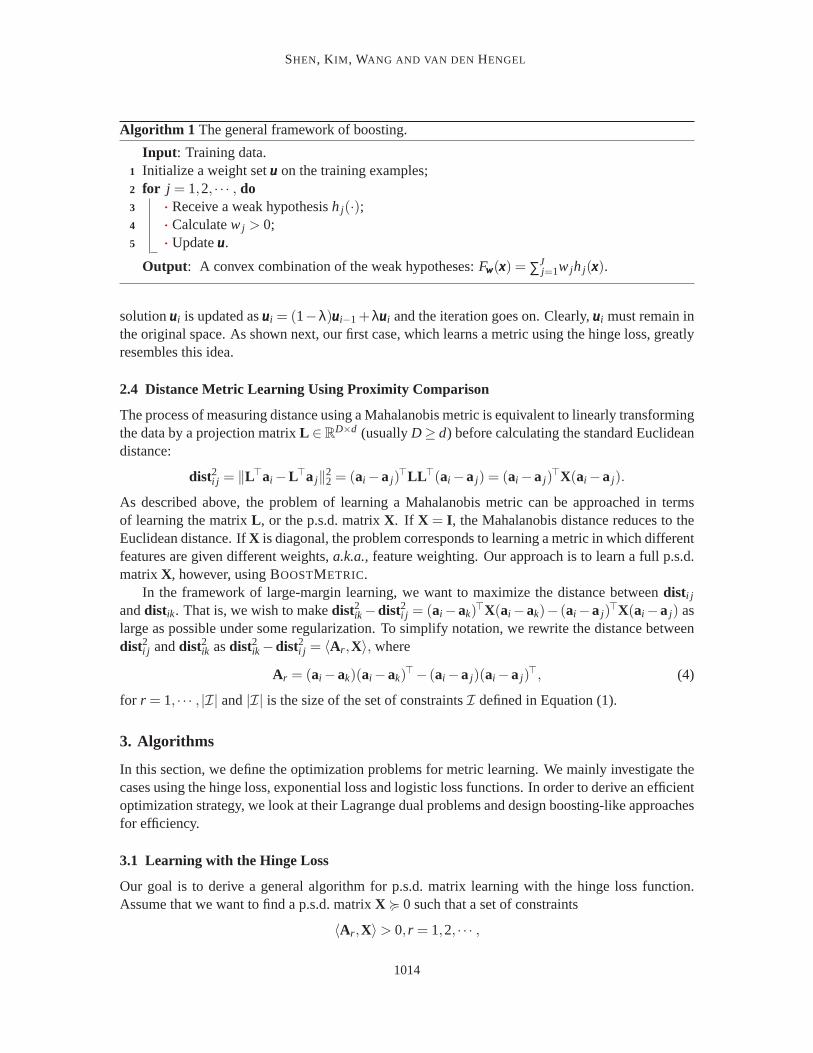
Algorithm 1 The general framework of boosting.

Input : Training data.Initialize a weight setuuu on the training examples;1

for j = 1,2, · · · , do2

··· Receive a weak hypothesish j(·);3

··· Calculatew j > 0;4

··· Updateuuu.5

Output : A convex combination of the weak hypotheses:Fwww(xxx) = ∑Jj=1w jh j(xxx).

solutionuuui is updated asuuui = (1−λ)uuui−1+λuuui and the iteration goes on. Clearly,uuui must remain inthe original space. As shown next, our first case, which learns a metric using the hinge loss, greatlyresembles this idea.

2.4 Distance Metric Learning Using Proximity Comparison

The process of measuring distance using a Mahalanobis metric is equivalent to linearly transformingthe data by a projection matrixL ∈R

D×d (usuallyD ≥ d) before calculating the standard Euclideandistance:

dist2i j = ‖L⊤ai −L⊤a j‖22 = (ai −a j)

⊤LL⊤(ai −a j) = (ai −a j)⊤X(ai −a j).

As described above, the problem of learning a Mahalanobis metric can be approached in termsof learning the matrixL , or the p.s.d. matrixX. If X = I , the Mahalanobis distance reduces to theEuclidean distance. IfX is diagonal, the problem corresponds to learning a metric in which differentfeatures are given different weights,a.k.a.,feature weighting. Our approach is to learn a full p.s.d.matrixX, however, using BOOSTMETRIC.

In the framework of large-margin learning, we want to maximize the distance betweendisti janddistik. That is, we wish to makedist2ik −dist2i j = (ai −ak)

⊤X(ai −ak)− (ai −a j)⊤X(ai −a j) as

large as possible under some regularization. To simplify notation, we rewrite the distance betweendist2i j anddist2ik asdist2ik −dist2i j = 〈Ar ,X〉, where

Ar = (ai −ak)(ai −ak)⊤− (ai −a j)(ai −a j)

⊤, (4)

for r = 1, · · · , |I| and|I| is the size of the set of constraintsI defined in Equation (1).

3. Algorithms

In this section, we define the optimization problems for metric learning. We mainly investigate thecases using the hinge loss, exponential loss and logistic loss functions. Inorder to derive an efficientoptimization strategy, we look at their Lagrange dual problems and design boosting-like approachesfor efficiency.

3.1 Learning with the Hinge Loss

Our goal is to derive a general algorithm for p.s.d. matrix learning with the hinge loss function.Assume that we want to find a p.s.d. matrixX < 0 such that a set of constraints

〈Ar ,X〉> 0, r = 1,2, · · · ,

1014


are satisfied aswell as possible. HereAr is as defined in (4). These constraints need not all bestrictly satisfied and thus we define the marginρr = 〈Ar ,X〉, ∀r.

Putting it into the maximum margin learning framework, we want to minimize the followingtrace norm regularized objective function:∑r F(〈Ar ,X〉)+vTr (X),with F(·) a convex loss functionand v a regularization constant. Here we have used the trace norm regularization. Of course aFrobenius norm regularization term can also be used here. Minimizing the Frobenius norm||X||2F,which is equivalent to minimize theℓ2 norm of the eigenvalues ofX, penalizes a solution that is faraway from the identity matrix. With the hinge loss, we can write the optimization problem as:

maxρ,X,ξξξ

ρ−v∑|I|r=1ξr , s.t.: 〈Ar ,X〉 ≥ ρ−ξr ,∀r;X < 0,Tr (X) = 1; ξξξ ≥ 000. (5)

HereTr (X) = 1 removes the scale ambiguity because the distance inequalities are scale invariant.We can decomposeX into: X = ∑J

j=1w jZ j , with w j > 0, Rank(Z j) = 1 andTr (Z j) = 1, ∀ j.So we have

〈Ar ,X〉=⟨Ar ,∑J

j=1w jZ j⟩= ∑J

j=1w j⟨Ar ,Z j

⟩= ∑J

j=1w jHr j = Hr:www,∀r. (6)

HereHr j is a shorthand forHr j =⟨Ar ,Z j

⟩. Clearly,Tr (X) = 111⊤www. Using Theorem 4, we replace

the p.s.d. conic constraint in the primal (5) with a linear convex combination of rank-one unitarymatrices:X = ∑ jw jZ j , and 111⊤www= 1. SubstitutingX in (5), we have

maxρ,www,ξξξ

ρ−v∑|I|r=1ξr , s.t.: Hr:www≥ ρ−ξr ,(r = 1, . . . , |I|);www≥ 000,111⊤www= 1; ξξξ ≥ 000. (7)

The Lagrange dual problem of the above linear programming problem (7)is easily derived:

minπ,uuu

π s.t.: ∑|I|r=1urHr: ≤ π111⊤;111⊤uuu= 1,000≤ uuu≤ v111.

We can then use column generation to solve the original problem iteratively bylooking at both theprimal and dual problems. See Shen et al. (2008) for the algorithmic details.In this work we aremore interested in smooth loss functions such as the exponential loss and logistic loss, as presentedin the sequel.

3.2 Learning with the Exponential Loss

By employing the exponential loss, we want to optimize

minX,ρρρ

log(

∑|I|r=1exp(−ρr)

)+vTr (X)

s.t.:ρr = 〈Ar ,X〉, r = 1, · · · , |I|, X < 0. (8)

Note that: 1) We are proposing a logarithmic version of the sum of exponential loss. This transformdoes not change the original optimization problem of sum of exponential loss because the logarith-mic function is strictly monotonically increasing. 2) A regularization termTr (X) has been applied.Without this regularization, one can always multiplyX by an arbitrarily large scale factor in orderto make the exponential loss approach zero in the case of all constraints being satisfied. This trace-norm regularization may also lead to low-rank solutions. 3) An auxiliary variableρr , r = 1, . . . mustbe introduced for deriving a meaningful dual problem, as we show later.

1015


We now derive the Lagrange dual of the problem that we are interested in. The original problem(8) now becomes

minρρρ,www

log(


)+v111⊤www

s.t.:ρr = Hr:www, r = 1, · · · , |I|; www≥ 000. (9)

We have used the Equation (6). In order to derive its dual, we write its Lagrangian

L(www,ρρρ,uuu) = log(


)+v111⊤www+∑|I|

r=1ur(ρr −Hr:www)− ppp⊤www,

with ppp≥ 0. The dual problem is obtained by finding the saddle point ofL; that is, supuuu infwww,ρρρ L.

infwww,ρρρ

L = infρρρ

L1︷︸︸︷

log(


)+uuu⊤ρρρ+ inf

www

L2︷︸︸︷

(v111⊤−∑|I|r=1urHr: − ppp⊤)www (10)

=−∑|I|r=1ur logur .

The infimum ofL1 is found by setting its first derivative to zero and we have:

infρρρ

L1 =

{

−∑rur logur if uuu≥ 000,111⊤uuu= 1,

−∞ otherwise.

The infimum is Shannon entropy.L2 is linear inwww, hence it must be 000. It leads to

∑|I|r=1urHr: ≤ v111⊤. (11)

The Lagrange dual problem of (9) is an entropy maximization problem, whichwrites

maxuuu

−∑|I|r=1ur logur , s.t.: uuu≥ 000,111⊤uuu= 1,and (11). (12)

Weak and strong duality hold under mild conditions (Boyd and Vandenberghe, 2004). That means,one can usually solve one problem from the other. The KKT conditions link the optimal betweenthese two problems. In our case, it is

u⋆r =exp(−ρ⋆

r )

∑|I|k=1exp(−ρ⋆

k),∀r. (13)

While it is possible to devise a totally-corrective column generation based optimization proce-dure for solving our problem as the case of LPBoost (Demiriz et al., 2002), we are more interested inconsideringone-at-a-timecoordinate-wise descent algorithms, as the case of AdaBoost (Schapire,1999). Let us start from some basic knowledge of column generation because our coordinate descentstrategy is inspired by column generation.

If we know all the basesZ j ( j = 1. . .J) and hence the entire matrixH is known. Then eitherthe primal (9) or the dual (12) can be trivially solved (at least in theory) because both are convexoptimization problems. We can solve them in polynomial time. Especially the primal problem isconvex minimization with simple nonnegativeness constraints. Off-the-shelf software like LBFGS-B (Zhu et al., 1997) can be used for this purpose. Unfortunately, in practice, we do not access all

1016


the bases: the possibility ofZ is infinite. In convex optimization, column generation is a techniquethat is designed for solving this difficulty.

Column generation was originally advocated for solving large scale linear programs (Lubbeckeand Desrosiers, 2005). Column generation is based on the fact that fora linear program, the numberof non-zero variables of the optimal solution is equal to the number of constraints. Therefore,although the number of possible variables may be large, we only need a small subset of these inthe optimal solution. For a general convex problem, we can use column generation to obtain anapproximatesolution. It works by only considering a small subset of the entire variableset. Onceit is solved, we ask the question:“Are there any other variables that can beincluded to improvethe solution?”. So we must be able to solve the subproblem: given a set of dual values, one eitheridentifies a variable that has a favorable reduced cost, or indicates that such a variable does not exist.Essentially, column generation finds the variables with negative reduced costs without explicitlyenumerating all variables.

Instead of directly solving the primal problem (9), we find the most violated constraint in thedual (12) iteratively for the current solution and adds this constraint to the optimization problem.For this purpose, we need to solve

Z = argmaxZ{

∑|I|r=1ur

⟨Ar ,Z

⟩, s.t.: Z ∈ Ψ1

}

. (14)

We discuss how to efficiently solve (14) later. Now we move on to derive a coordinate descentoptimization procedure.

3.3 Coordinate Descent Optimization

We show how an AdaBoost-like optimization procedure can be derived.

3.3.1 OPTIMIZING FOR w j

Since we are interested in theone-at-a-timecoordinate-wise optimization, we keepw1, w2, . . . , w j−1

fixed when solving forw j . The cost function of the primal problem is (in the following derivation,we drop those terms irrelevant to the variablew j )

Cp(w j) = log[

∑|I|r=1exp(−ρ j−1

r ) ·exp(−Hr j w j)]+vwj .

Clearly,Cp is convex inw j and hence there is only one minimum that is also globally optimal. Thefirst derivative ofCp w.r.t. w j vanishes at optimality, which results in

∑|I|r=1(Hr j −v)u j−1

r exp(−w jHr j ) = 0. (15)

If Hr j is discrete, such as{+1,−1} in standard AdaBoost, we can obtain a closed-form solutionsimilar to AdaBoost. Unfortunately in our case,Hr j can be any real value. We instead use bisectionto search for the optimalw j . The bisection method is one of the root-finding algorithms. It repeat-edly divides an interval in half and then selects the subinterval in which a root exists. Bisection isa simple and robust, although it is not the fastest algorithm for root-finding.Algorithm 2 gives thebisection procedure. We have used the fact that the l.h.s. of (15) must bepositive atwl . Otherwiseno solution can be found. Whenw j = 0, clearly the l.h.s. of (15) is positive.

1017


Algorithm 2 Bisection search forw j .

Input : An interval[wl ,wu] known to contain the optimal value ofw j and convergencetoleranceε > 0.

repeat1

··· w j = 0.5(wl +wu);2

··· if l.h.s.of (15)> 0 then3

wl = w j ;4

else5

wu = w j .6

until wu−wl < ε ;7

Output : w j .

3.3.2 UPDATING uuu

The rule for updatinguuu can be easily obtained from (13). At iterationj, we have

u jr ∝ exp(−ρ j

r ) ∝ u j−1r exp(−Hr j w j), and∑|I|

r=1u jr = 1,

derived from (13). So oncew j is calculated, we can updateuuu as

u jr =

u j−1r exp(−Hr j w j)

z, r = 1, . . . , |I|, (16)

wherez is a normalization factor so that∑|I|r=1u j

r = 1. This is exactly the same as AdaBoost.

3.4 The Base Learning Algorithm

In this section, we show that the optimization problem (14) can be exactly and efficiently solvedusing eigenvalue-decomposition (EVD).

FromZ < 0 andRank(Z) = 1, we know thatZ has the format:Z = vvvvvv⊤, vvv∈RD; andTr (Z) = 1

means‖vvv‖2 = 1. We have⟨

∑|I|r=1urAr ,Z

⟩= vvv

(

∑|I|r=1urAr

)vvv⊤.

By denoting

A = ∑|I|r=1urAr , (17)

the base learning optimization equals:

maxvvv

vvv⊤Avvv, s.t.:‖vvv‖2 = 1. (18)

It is clear that the largest eigenvalue ofA, λmax(A), and its corresponding eigenvectorvvv1 gives thesolution to the above problem. Note thatA is symmetric.

λmax(A) is also used as one of the stopping criteria of the algorithm. Form the condition (11),λmax(A)< v means that we are not able to find a new base matrixZ that violates (11)—the algorithmconverges.

1018


Algorithm 3 Positive semidefinite matrix learning with stage-wise boosting.

Input :

• Training set triplets(ai ,a j ,ak) ∈ I; ComputeAr , r = 1,2, · · · , using (4).

• J: maximum number of iterations;

• (optional) regularization parameterv; We may simply setv to a very small value, forexample, 10−7.

Initialize : u0r =

1|I| , r = 1· · · |I|;1

for j = 1,2, · · · ,J do2

··· Find a new baseZ j by finding the largest eigenvalue (λmax(A)) and its eigenvector of3

A in (17);··· if λmax(A)< v then4

break (converged);5

··· Computew j using Algorithm 2;6

··· Updateuuu to obtainu jr , r = 1, · · · |I| using (16);7

Output : The final p.s.d. matrixX ∈ RD×D, X = ∑J

j=1w jZ j .

Eigenvalue decompositions is one of the main computational costs in our algorithm.Thereare approximate eigenvalue solvers, which guarantee that for a symmetric matrix U and anyε >0, a vectorvvv is found such thatvvv⊤Uvvv ≥ λmax− ε. To approximately find the largest eigenvalueand eigenvector can be very efficient using Lanczos or power method.We can use the MATLABfunction eigs to calculate the largest eigenvector, which calls mex files of ARPACK. ARPACK isa collection of Fortran subroutines designed to solve large scale eigenvalue problems. When theinput matrix is symmetric, this software uses a variant of the Lanczos process called the implicitlyrestarted Lanczos method.

Another way to reduce the time for computing the leading eigenvector is to computean approx-imate EVD by a fast Monte Carlo algorithm such as the linear time SVD algorithm developed inDrineas et al. (2004).

We summarize our main algorithmic results in Algorithm 3.

3.5 Learning with the Logistic Loss

We have considered the exponential loss in the last content. The proposed framework is so generalthat it can also accommodate other convex loss functions. Here we consider the logistic loss, whichpenalizes mis-classifications with more moderate penalties than the exponential loss. It is believedon noisy data, the logistic loss may achieve better classification performance.

With the same settings as in the case of the exponential loss, we can write our optimizationproblem as

minρρρ,www

∑|I|r=1logit(ρr)+v1⊤www

s.t.:ρr = Hr:www, r = 1, · · · , |I|,www≥ 0. (19)

1019


Here logit(·) is the logistic loss defined as logit(z) = log(1+ exp(−z)). Similarly, we derive itsLagrange dual as

minuuu

∑|I|r=1logit∗(−ur)

s.t.:∑|I|r=1urHr: ≤ v1⊤,

where logit∗(·) is the Fenchel conjugate function of logit(·), defined as

logit∗(−u) = ulog(u)+(1−u) log(1−u),

when 0≤ u≤ 1, and∞ otherwise. So the Fenchel conjugate of logit(·) is the binary entropy function.We have reversed the sign ofuuu when deriving the dual.

Again, according to the KKT conditions, we have

u⋆r =exp(−ρ⋆

r )

1+exp(−ρ⋆r ), ∀r, (20)

at optimality. From (20) we can also see thatu must be in(0,1).Similarly, we want to optimize the primal cost function in a coordinate descent way. First, let

us find the relationship betweenu jr andu j−1

r . Here j is the iteration index. From (20), it is trivial toobtain

u jr =

1

(1/u j−1r −1)exp(Hr j w j)+1

, ∀r. (21)

The optimization ofw j can be solved by looking for the root of

∑|I|r=1Hr j u

jr −v= 0, (22)

whereu jr is a function ofw j as defined in (21).

Therefore, in the case of the logistic loss, to findw j , we modify the bisection search of Algo-rithm 2:

• Line 3: if l.h.s.o f (22)> 0 then . . .

and Line 7 of Algorithm 3:

• Line 7: Updateuuu using (21).

3.6 Totally Corrective Optimization

In this section, we derive a totally-corrective version of BOOSTMETRIC, similar to the case of Total-Boost (Warmuth et al., 2006; Shen and Li, 2010) for classification, in the sense that the coefficientsof all weak learners are updated at each iteration.

Unlike the stage-wise optimization, here we do not need to keep previous weights of weaklearnersw1,w2, . . . ,w j−1. Instead, the weights of all the selected weak learnersw1,w2, . . . ,w j areupdated at each iterationj. As discussed, our learning procedure is able to employ various lossfunctions such as the hinge loss, exponential loss or logistic loss. To devise a totally-correctiveoptimization procedure for solving our problem efficiently, we need to ensure the object function

1020


Algorithm 4 Positive semidefinite matrix learning with totally corrective boosting.

Input :

• Training set triplets(ai ,a j ,ak) ∈ I; ComputeAr , r = 1,2, · · · , using (4).

• J: maximum number of iterations;

• Regularization parameterv.

Initialize : u0r =

1|I| , r = 1· · · |I|;1

for j = 1,2, · · · ,J do2

··· Find a new baseZ j by finding the largest eigenvalue (λmax(A)) and its eigenvector of3

A in (17);··· if λmax(A)< v then4

break (converged);5

··· Optimize forw1,w2, · · · ,w j by solving the primal problem (9) when the exponential6

loss is used or (19) when the logistic loss is used;··· Updateuuu to obtainu j

r , r = 1, · · · |I| using (13) (exponential loss) or (20) (logistic loss);7

Output : The final p.s.d. matrixX ∈ RD×D, X = ∑J

j=1w jZ j .

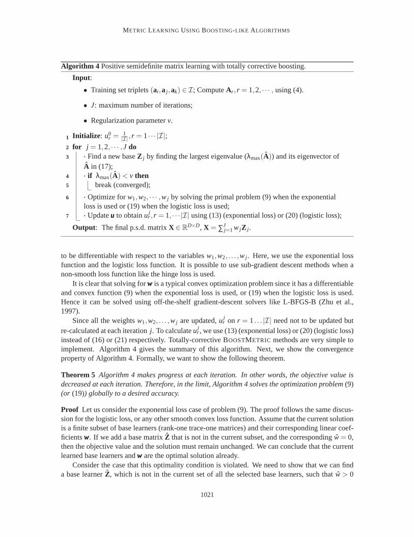
to be differentiable with respect to the variablesw1,w2, . . . ,w j . Here, we use the exponential lossfunction and the logistic loss function. It is possible to use sub-gradient descent methods when anon-smooth loss function like the hinge loss is used.

It is clear that solving forwww is a typical convex optimization problem since it has a differentiableand convex function (9) when the exponential loss is used, or (19) when the logistic loss is used.Hence it can be solved using off-the-shelf gradient-descent solverslike L-BFGS-B (Zhu et al.,1997).

Since all the weightsw1,w2, . . . ,w j are updated,u jr on r = 1. . . |I| need not to be updated but

re-calculated at each iterationj. To calculateu jr , we use (13) (exponential loss) or (20) (logistic loss)

instead of (16) or (21) respectively. Totally-corrective BOOSTMETRIC methods are very simple toimplement. Algorithm 4 gives the summary of this algorithm. Next, we show the convergenceproperty of Algorithm 4. Formally, we want to show the following theorem.

Theorem 5 Algorithm 4 makes progress at each iteration. In other words, the objective value isdecreased at each iteration. Therefore, in the limit, Algorithm 4 solves the optimization problem(9)(or (19)) globally to a desired accuracy.

Proof Let us consider the exponential loss case of problem (9). The proof follows the same discus-sion for the logistic loss, or any other smooth convex loss function. Assume that the current solutionis a finite subset of base learners (rank-one trace-one matrices) and their corresponding linear coef-ficientswww. If we add a base matrixZ that is not in the current subset, and the corresponding ˆw= 0,then the objective value and the solution must remain unchanged. We can conclude that the currentlearned base learners andwww are the optimal solution already.

Consider the case that this optimality condition is violated. We need to show that wecan finda base learnerZ, which is not in the current set of all the selected base learners, such that w > 0

1021


holds. Now assume thatZ is the base learner found by solving (18), and the convergence condition

λmax(A)≤ v is not satisfied. So, we haveλmax(A) =⟨

∑|I|r=1urAr , Z

⟩

> v.

If, after this weak learnerZ is added into the primal problem, the primal solution remainsunchanged, that is, the corresponding ˆw= 0, then from the optimality condition thatL2 in (10) must

be zero, we know that ˆp= v−⟨

∑|I|r=1urAr , Z

⟩

< 0. This contradicts the fact the Lagrange multiplier

p≥ 0.

We can conclude that after the base learnerZ is added into the primal problem, its correspondingw must admit a positive value. It means that one more free variable is added intothe problem andre-solving the primal problem would reduce the objective value. Hence a strict decrease in theobjective is guaranteed. So Algorithm 4 makes progress at each iteration.

Furthermore, as the optimization problems involved are all convex, there areno local optimalsolutions. Therefore Algorithm 4 is guaranteed to converge to the global solution.

Note that the above proof establishes the convergence of Algorithm 4 butit remains unclearabout the convergence rate.

3.7 Multi-passBOOSTMETRIC

In this section, we show that BOOSTMETRIC can use multi-pass learning to enhance the perfor-mance.

Our BOOSTMETRIC uses training set triplets(ai ,a j ,ak) ∈ I as input for training. The Maha-lanobis distance metricX can be viewed as a linear transformation in the Euclidean space by project-ing the data using matrixL (X = LL⊤). That is, nearest neighbors of samples using Mahalanobisdistance metricX are the same as nearest neighbors using Euclidean distance in the transformedspace. BOOSTMETRIC assumes that the triplets of input training set approximately represent theactual nearest neighbors of samples in the transformed space defined by the Mahalanobis metric.However, even though the triplets of BOOSTMETRIC consist of nearest neighbors of the originaltraining samples, generated triplets are not exactly the same as the actual nearest neighbors of train-ing samples in the transformed space byL .

We can refine the results of BOOSTMETRIC iteratively, as in the multiple-pass LMNN (Wein-berger and Saul, 2009): BOOSTMETRIC can estimate the triplets in the transformed space undera multiple-pass procedure as close to actual triplets as possible. The rule for multi-pass BOOST-METRIC is simple. At each passp (p= 1,2, · · ·), we decompose the learned Mahalanobis distancemetric Xp−1 of previous pass into transformation matrixL p. The initial matrixL1 is an identitymatrix. Then we generate the training set triplets from the set of points{L⊤a1, . . . ,L⊤am} whereL = L1 ·L2 · · · ·L p. The final Mahalanobis distance metricX becomesLL⊤ in Multi-pass BOOST-METRIC.

4. Experiments

In this section, we present experiments on data visualization, classification and image retrieval tasks.

1022


MN

IST

US

PS

Lette

rsyF

aces

bal

win

eiri

s

#of

sam

ples

70,0

0011

,000

20,0

002,

414

625

178

150

#of

trip

lets

450,

000

69,3

0094

,500

15,2

103,

942

1,12

594

5di

men

sion

784

256

161,

024

413

4di

men

sion

afte

rP

CA

164

6030

0#

ofsa

mpl

esfo

rtr

aini

ng50

,000

7,70

010

,500

1,69

043

812

510

5#

cros

sva

lidat

ion

sam

ples

10,0

001,

650

4,50

036

294

2723

#te

stsa

mpl

es10

,000

1,65

05,

000

362

9326

22#

ofcl

asse

s10

1026

383

33

#of

runs

110

110

1010

10

ErrorRates

Euc

lidea

n3.

194.

78(0

.40)

5.42

28.0

7(2

.07)

18.6

0(3

.96)

28.0

8(7

.49)

3.64

(4.1

8)P

CA

3.10

3.49

(0.6

2)28

.65

(2.1

8)LD

A8.

766.

96(0

.68)

4.44

5.08

(1.1

5)12

.58

(2.3

8)0.

77(1

.62)

3.18

(3.0

7)R

CA

7.85

5.35

(0.5

2)4.

647.

65(1

.08)

17.4

2(3

.58)

0.38

(1.2

2)3.

18(3

.07)

NC

A18

.28

(3.5

8)28

.08

(7.4

9)3.

18(3

.74)

LMN

N2.

303.

49(0

.62)

3.82

14.7

5(1

2.11

)12

.04

(5.5

9)3.

46(3

.82)

3.64

(2.8

7)IT

ML

2.80

3.85

(1.1

3)7.

2019

.39

(2.1

1)10

.11

(4.0

6)28

.46

(8.3

5)3.

64(3

.59)

Boo

stM

etric

-E2.

652.

53(0

.47)

3.06

6.91

(1.9

0)10

.11

(3.4

5)3.

08(3

.53)

3.18

(3.7

4)B

oost

Met

ric-E

,MP

2.62

2.24

(0.4

0)2.

806.

77(1

.77)

10.2

2(4

.43)

1.92

(2.0

3)3.

18(4

.31)

Boo

stM

etric

-E,T

C2.

202.

25(0

.51)

2.82

7.13

(1.4

0)10

.22

(2.3

9)4.

23(3

.82)

3.18

(3.0

7)B

oost

Met

ric-E

,MP,

TC

2.34

2.23

(0.3

4)3.

747.

29(1

.58)

10.3

2(3

.09)

2.69

(3.1

7)3.

18(4

.31)

Boo

stM

etric

-L2.

662.

38(0

.31)

2.80

6.93

(1.5

9)9.

89(3

.12)

3.08

(3.0

3)3.

18(3

.74)

Boo

stM

etric

-L,M

P2.

722.

22(0

.31)

2.70

6.66

(1.3

5)10

.22

(4.2

5)1.

15(1

.86)

3.18

(4.3

1)B

oost

Met

ric-L

,TC

2.10

2.13

(0.4

1)2.

487.

71(1

.68)

9.57

(3.1

8)3.

85(4

.05)

3.64

(2.8

7)B

oost

Met

ric-L

,MP,

TC

2.11

2.10

(0.4

2)2.

367.

15(1

.32)

8.49

(3.7

1)3.

08(3

.03)

2.73

(2.3

5)

Comp.Time

LMN

N10

.98h

20s

1249

s89

6s5s

2s2s

ITM

L0.

41h

72s

55s

5970

s8s

4s4s

Boo

stM

etric

-E2.

83h

144s

3s62

8sle

ssth

an1s

2sle

ssth

an1s

Boo

stM

etric

-L0.

89h

65s

34s

256s

less

than

1s2s

less

than

1s

Tabl

e1:

Com

paris

onof

test

clas

sific

atio

ner

ror

rate

s(%

)of

a3-

near

estn

eigh

bor

clas

sifie

ron

benc

hmar

kda

tase

ts.

Res

ults

ofN

CA

are

not

avai

labl

eei

ther

beca

use

the

algo

rithm

does

not

conv

erge

ordu

eto

the

out-

of-m

emor

ypr

oble

m.

Boo

stM

etric

-Ein

dica

tes

BO

OS

T-M

ET

RIC

with

the

expo

nent

iall

oss

and

Boo

stM

etric

-Lis

BO

OS

TME

TR

ICw

ithth

elo

gist

iclo

ss;

both

use

stag

e-w

ise

optim

izat

ion.

“MP

”m

eans

Mul

tiple

-Pas

sBO

OS

TME

TR

ICan

d“T

C”

isB

OO

STM

ET

RIC

with

tota

llyco

rrec

tive

optim

izat

ion.

We

repo

rtco

mpu

ta-

tiona

ltim

eas

wel

l.

1023


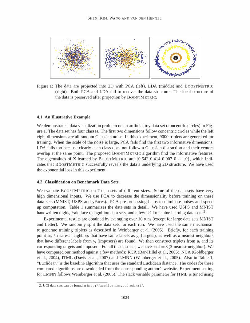
Figure 1: The data are projected into 2D with PCA (left), LDA (middle) and BOOSTMETRIC

(right). Both PCA and LDA fail to recover the data structure. The local structure ofthe data is preserved after projection by BOOSTMETRIC.

4.1 An Illustrative Example

We demonstrate a data visualization problem on an artificial toy data set (concentric circles) in Fig-ure 1. The data set has four classes. The first two dimensions follow concentric circles while the lefteight dimensions are all random Gaussian noise. In this experiment, 9000 triplets are generated fortraining. When the scale of the noise is large, PCA fails find the first two informative dimensions.LDA fails too because clearly each class does not follow a Gaussian distraction and their centersoverlap at the same point. The proposed BOOSTMETRIC algorithm find the informative features.The eigenvalues ofX learned by BOOSTMETRIC are{0.542,0.414,0.007,0, · · · ,0}, which indi-cates that BOOSTMETRIC successfully reveals the data’s underlying 2D structure. We have usedthe exponential loss in this experiment.

4.2 Classification on Benchmark Data Sets

We evaluate BOOSTMETRIC on 7 data sets of different sizes. Some of the data sets have veryhigh dimensional inputs. We use PCA to decrease the dimensionality before training on thesedata sets (MNIST, USPS and yFaces). PCA pre-processing helps to eliminate noises and speedup computation. Table 1 summarizes the data sets in detail. We have used USPS and MNISThandwritten digits, Yale face recognition data sets, and a few UCI machine learning data sets.2

Experimental results are obtained by averaging over 10 runs (except for large data sets MNISTand Letter). We randomly split the data sets for each run. We have used thesame mechanismto generate training triplets as described in Weinberger et al. (2005). Briefly, for each trainingpoint ai , k nearest neighbors that have same labels asyi (targets), as well ask nearest neighborsthat have different labels fromyi (imposers) are found. We then construct triplets fromai and itscorresponding targets and imposers. For all the data sets, we have setk= 3 (3-nearest-neighbor). Wehave compared our method against a few methods: RCA (Bar-Hillel et al., 2005), NCA (Goldbergeret al., 2004), ITML (Davis et al., 2007) and LMNN (Weinberger et al., 2005). Also in Table 1,“Euclidean” is the baseline algorithm that uses the standard Euclidean distance. The codes for thesecompared algorithms are downloaded from the corresponding author’s website. Experiment settingfor LMNN follows Weinberger et al. (2005). The slack variable parameter for ITML is tuned using

2. UCI data sets can be found athttp://archive.ics.uci.edu/ml/.

1024


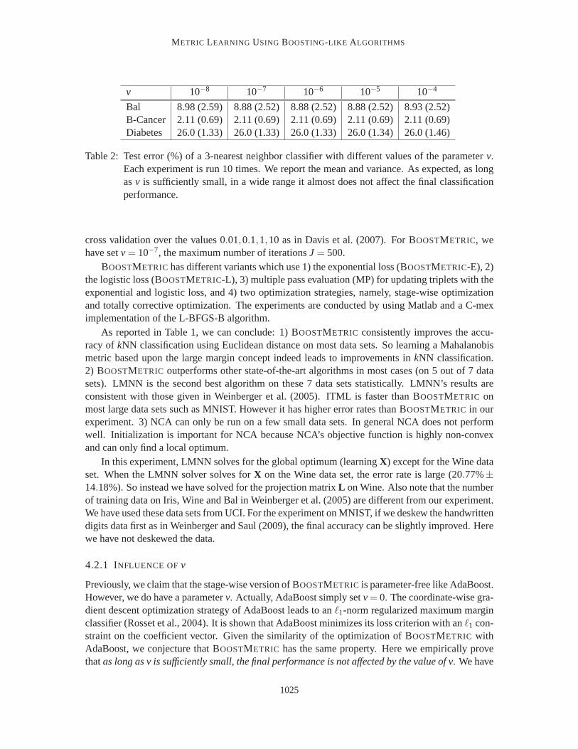
v 10−8 10−7 10−6 10−5 10−4

Bal 8.98 (2.59) 8.88 (2.52) 8.88 (2.52) 8.88 (2.52) 8.93 (2.52)B-Cancer 2.11 (0.69) 2.11 (0.69) 2.11 (0.69) 2.11 (0.69) 2.11 (0.69)Diabetes 26.0 (1.33) 26.0 (1.33) 26.0 (1.33) 26.0 (1.34) 26.0 (1.46)

Table 2: Test error (%) of a 3-nearest neighbor classifier with different values of the parameterv.Each experiment is run 10 times. We report the mean and variance. As expected, as longasv is sufficiently small, in a wide range it almost does not affect the final classificationperformance.

cross validation over the values 0.01,0.1,1,10 as in Davis et al. (2007). For BOOSTMETRIC, wehave setv= 10−7, the maximum number of iterationsJ = 500.

BOOSTMETRIC has different variants which use 1) the exponential loss (BOOSTMETRIC-E), 2)the logistic loss (BOOSTMETRIC-L), 3) multiple pass evaluation (MP) for updating triplets with theexponential and logistic loss, and 4) two optimization strategies, namely, stage-wise optimizationand totally corrective optimization. The experiments are conducted by using Matlab and a C-meximplementation of the L-BFGS-B algorithm.

As reported in Table 1, we can conclude: 1) BOOSTMETRIC consistently improves the accu-racy ofkNN classification using Euclidean distance on most data sets. So learning a Mahalanobismetric based upon the large margin concept indeed leads to improvements inkNN classification.2) BOOSTMETRIC outperforms other state-of-the-art algorithms in most cases (on 5 out of 7datasets). LMNN is the second best algorithm on these 7 data sets statistically. LMNN’s results areconsistent with those given in Weinberger et al. (2005). ITML is faster than BOOSTMETRIC onmost large data sets such as MNIST. However it has higher error rates than BOOSTMETRIC in ourexperiment. 3) NCA can only be run on a few small data sets. In general NCA does not performwell. Initialization is important for NCA because NCA’s objective function is highly non-convexand can only find a local optimum.

In this experiment, LMNN solves for the global optimum (learningX) except for the Wine dataset. When the LMNN solver solves forX on the Wine data set, the error rate is large (20.77%±14.18%). So instead we have solved for the projection matrixL on Wine. Also note that the numberof training data on Iris, Wine and Bal in Weinberger et al. (2005) are different from our experiment.We have used these data sets from UCI. For the experiment on MNIST, if we deskew the handwrittendigits data first as in Weinberger and Saul (2009), the final accuracy can be slightly improved. Herewe have not deskewed the data.

4.2.1 INFLUENCE OFv

Previously, we claim that the stage-wise version of BOOSTMETRIC is parameter-free like AdaBoost.However, we do have a parameterv. Actually, AdaBoost simply setv= 0. The coordinate-wise gra-dient descent optimization strategy of AdaBoost leads to anℓ1-norm regularized maximum marginclassifier (Rosset et al., 2004). It is shown that AdaBoost minimizes its losscriterion with anℓ1 con-straint on the coefficient vector. Given the similarity of the optimization of BOOSTMETRIC withAdaBoost, we conjecture that BOOSTMETRIC has the same property. Here we empirically provethatas long as v is sufficiently small, the final performance is not affected by thevalue of v. We have

1025


setv from 10−8 to 10−4 and run BOOSTMETRIC on 3 UCI data sets. Table 2 reports the final 3NNclassification error with differentv. The results are nearly identical.

For the totally corrective version of BOOSTMETRIC, similar results are observed. Actually forLMNN, it was also reported that the regularization parameter does not have a significant impact onthe final results in a wide range (Weinberger and Saul, 2009).

4.2.2 COMPUTATIONAL TIME

As we discussed, one major issue in learning a Mahalanobis distance is heavy computational costbecause of the semidefiniteness constraint.

We have shown the running time of the proposed algorithm in Table 1 for the classificationtasks.3 Our algorithm is generally fast. Our algorithm involves matrix operations and an EVD forfinding its largest eigenvalue and its corresponding eigenvector. The time complexity of this EVDis O(D2) with D the input dimensions. We compare our algorithm’s running time with LMNN inFigure 2 on the artificial data set (concentric circles). Our algorithm is stage-wise BOOSTMETRIC

with the exponential loss. We vary the input dimensions from 50 to 1000 and keep the numberof triplets fixed to 250. LMNN does not use standard interior-point SDP solvers, which do notscale well. Instead LMNN heuristically combines sub-gradient descent in both the matricesL andX. At each iteration,X is projected back onto the p.s.d. cone using EVD. So a full EVD withtime complexityO(D3) is needed. Note that LMNN is much faster than SDP solvers like CSDP(Borchers, 1999). As seen from Figure 2, when the input dimensions are low, BOOSTMETRIC

is comparable to LMNN. As expected, when the input dimensions become large, BOOSTMETRIC

is significantly faster than LMNN. Note that our implementation is in Matlab. Improvements areexpected if implemented in C/C++.

4.3 Visual Object Categorization

In the following experiments, unless otherwise specified, BOOSTMETRIC means the stage-wiseBOOSTMETRIC with the exponential loss.

The proposed BOOSTMETRIC and the LMNN are further compared on visual object cate-gorization tasks. The first experiment uses four classes of the Caltech-101 object recognitiondatabase (Fei-Fei et al., 2006), including Motorbikes (798 images), Airplanes (800), Faces (435),and Background-Google (520). The task is to label each image according to the presence of a par-ticular object. This experiment involves both object categorization (Motorbikes versus Airplanes)and object retrieval (Faces versus Background-Google) problems.In the second experiment, wecompare the two methods on the MSRC data set including 240 images.4 The objects in the imagescan be categorized into nine classes, includingbuilding, grass, tree, cow, sky, airplane, face, carand bicycle. Different from the first experiment, each image in this database often contains multipleobjects. The regions corresponding to each object have been manually pre-segmented, and the taskis to label each region according to the presence of a particular object. Some examples are shownin Figure 3.

3. We have run all the experiments on a desktop with an Intel CoreTM2 Duo CPU, 4G RAM and Matlab 7.7 (64-bitversion).

4. Seehttp://research.microsoft.com/en-us/projects/objectclassrecognition/.

1026


0 200 400 600 800 10000

100

200

300

400

500

600

700

800

input dimensions

CP

U ti

me

per

run

(sec

onds

)

BoostMetric

LMNN

Figure 2: Computation time of the proposed BOOSTMETRIC (stage-wise, exponential loss) and theLMNN method versus the input data’s dimensions on an artificial data set. BOOSTMET-RIC is faster than LMNN with large input dimensions because at each iteration BOOST-METRIC only needs to calculate the largest eigenvector and LMNN needs a full eigen-decomposition.

Figure 3: Examples of the images in the MSRC data set and the pre-segmented regions labeledusing different colors.

4.3.1 EXPERIMENT ON THECALTECH-101 DATA SET

For each image of the four classes, a number of interest regions are identified by the Harris-affinedetector (Mikolajczyk and Schmid, 2004) and each region is characterized by the SIFT descrip-tor (Lowe, 2004). The total number of interest regions extracted from the four classes are about134,000, 84,000, 57,000, and 293,000, respectively. To accumulate statistics, the images of twoinvolved object classes are randomly split as 10 pairs of training/test subsets. Restricted to the im-ages in a training subset (those in a test subset are only used for test), their local descriptors areclustered to form visual words by usingk-means clustering. Each image is then represented by ahistogram containing the number of occurrences of each visual word.

1027


dim.: 100D 200D0

5

10

15

20

Tes

t err

or o

f 3−

near

est n

eigh

bor

(%)

Euclidean

LMNN

BoostMetric

1000 2000 3000 4000 5000 6000 7000 8000 90002.5

3

3.5

4

4.5

5

5.5

# of triplets

Tes

t err

or o

f 3−

near

est n

eigh

bor

(%)

Figure 4: Test error (3-nearest neighbor) of BOOSTMETRIC on the Motorbikes versus Airplanesdata sets. The second plot shows the test error against the number of training triplets witha 100-word codebook.

Motorbikes versus AirplanesThis experiment discriminates the images of a motorbike fromthose of an airplane. In each of the 10 pairs of training/test subsets, there are 959 training imagesand 639 test images. Two visual codebooks of size 100 and 200 are used, respectively. With theresulting histograms, the proposed BOOSTMETRIC and the LMNN are learned on a training subsetand evaluated on the corresponding test subset. Their averaged classification error rates are com-pared in Figure 4 (left). For both visual codebooks, the proposed BOOSTMETRIC achieves lowererror rates than the LMNN and the Euclidean distance, demonstrating its superior performance.We also apply a linear SVM classifier with its regularization parameter carefullytuned by 5-foldcross-validation. Its error rates are 3.87%± 0.69% and 3.00%± 0.72% on the two visual code-books, respectively. In contrast, a 3NN with BOOSTMETRIC has error rates 3.63%± 0.68% and2.96%± 0.59%. Hence, the performance of the proposed BOOSTMETRIC is comparable to thestate-of-the-art SVM classifier. Also, Figure 4 (right) plots the test errorof the BOOSTMETRIC

against the number of triplets for training. The general trend is that more triplets lead to smallererrors.

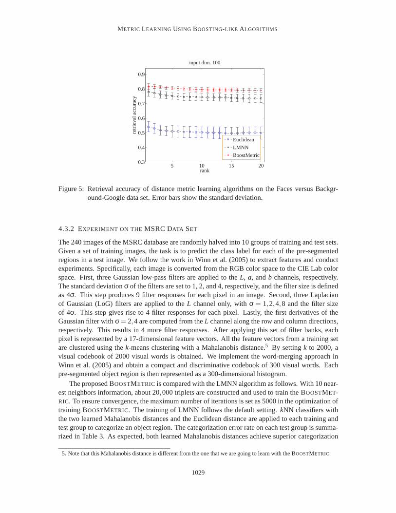
Faces versus Background-GoogleThis experiment uses the two object classes as a retrievalproblem. The target of retrieval is face images. The images in the class of Background-Google arerandomly collected from the Internet and they represent the non-targetclass. BOOSTMETRIC isfirst learned from a training subset and retrieval is conducted on the corresponding test subset. Ineach of the 10 training/test subsets, there are 573 training images and 382 test images. Again, twovisual codebooks of size 100 and 200 are used. Each face image in a test subset is used as a query,and its distances from other test images are calculated by the proposed BoostMetric, LMNN and theEuclidean distance, respectively. For each metric, thePrecisionof the retrieved top 5, 10, 15 and20 images are computed. ThePrecisionvalues from each query are averaged on this test subset andthen averaged over the 10 test subsets. The retrieval precision of these metrics is shown in Figure 5(with a codebook size 100). As we can see that the BOOSTMETRIC consistently attains the highestvalues on both visual codebooks, which again verifies its advantages over LMNN and Euclideandistance. With a codebook size 200, very similar results are obtained.

1028


5 10 15 200.3

0.4

0.5

0.6

0.7

0.8

0.9

rank

retr

ieva

l acc

urac

y

input dim. 100

Euclidean

LMNN

BoostMetric

Figure 5: Retrieval accuracy of distance metric learning algorithms on the Faces versus Backgr-ound-Google data set. Error bars show the standard deviation.

4.3.2 EXPERIMENT ON THEMSRC DATA SET

The 240 images of the MSRC database are randomly halved into 10 groups oftraining and test sets.Given a set of training images, the task is to predict the class label for eachof the pre-segmentedregions in a test image. We follow the work in Winn et al. (2005) to extract features and conductexperiments. Specifically, each image is converted from the RGB color space to the CIE Lab colorspace. First, three Gaussian low-pass filters are applied to theL, a, andb channels, respectively.The standard deviationσ of the filters are set to 1, 2, and 4, respectively, and the filter size is definedas 4σ. This step produces 9 filter responses for each pixel in an image. Second, three Laplacianof Gaussian (LoG) filters are applied to theL channel only, withσ = 1,2,4,8 and the filter sizeof 4σ. This step gives rise to 4 filter responses for each pixel. Lastly, the firstderivatives of theGaussian filter withσ = 2,4 are computed from theL channel along the row and column directions,respectively. This results in 4 more filter responses. After applying this set of filter banks, eachpixel is represented by a 17-dimensional feature vectors. All the feature vectors from a training setare clustered using thek-means clustering with a Mahalanobis distance.5 By settingk to 2000, avisual codebook of 2000 visual words is obtained. We implement the word-merging approach inWinn et al. (2005) and obtain a compact and discriminative codebook of 300 visual words. Eachpre-segmented object region is then represented as a 300-dimensional histogram.

The proposed BOOSTMETRIC is compared with the LMNN algorithm as follows. With 10 near-est neighbors information, about 20,000 triplets are constructed and used to train the BOOSTMET-RIC. To ensure convergence, the maximum number of iterations is set as 5000 inthe optimization oftraining BOOSTMETRIC. The training of LMNN follows the default setting.kNN classifiers withthe two learned Mahalanobis distances and the Euclidean distance are applied to each training andtest group to categorize an object region. The categorization error rateon each test group is summa-rized in Table 3. As expected, both learned Mahalanobis distances achieve superior categorization

5. Note that this Mahalanobis distance is different from the one that we aregoing to learn with the BOOSTMETRIC.

1029


group index Euclidean LMNN BOOSTMETRIC

1 9.19 6.71 4.592 5.78 3.97 3.253 6.69 2.97 2.604 5.54 3.69 4.435 6.52 5.80 4.356 7.30 4.01 3.287 7.75 2.21 2.588 7.20 4.17 4.559 6.13 3.07 4.2110 8.42 5.13 5.86

average: 7.05 4.17 3.97standard devision: 1.16 1.37 1.03

Table 3: Comparison of the categorization performance.

Figure 6: Four generated triplets based on the pairwise information provided by the LFW data set.For the three images in each triplet, the first two belong to the same individual and thethird one is a different individual.

performance to the Euclidean distance. Moreover, the proposed BOOSTMETRIC achieves betterperformance than the LMNN, as indicated by its lower average categorization error rate and thesmaller standard deviation. Also, thekNN classifier using the proposed BOOSTMETRIC achievescomparable or even higher categorization performance than those reported in Winn et al. (2005).Besides the categorization performance, we compare the computational efficiency of the BOOST-METRIC and the LMNN in learning a Mahalanobis distance. The computational time resultis basedon the Matlab codes for both methods. In this experiment, the average time costby the BOOSTMET-RIC for learning the Mahalanobis distance is 3.98 hours, whereas the LMNN takes about 8.06 hoursto complete this process. Hence, the proposed BOOSTMETRIC has a shorter training process thanthe LMNN method. This again demonstrates the computational advantage of the BOOSTMETRIC

over the LMNN method.

4.4 Unconstrained Face Recognition

We use the “labeled faces in the wild” (LFW) data set (Huang et al., 2007) for face recognition inthis experiment.

1030


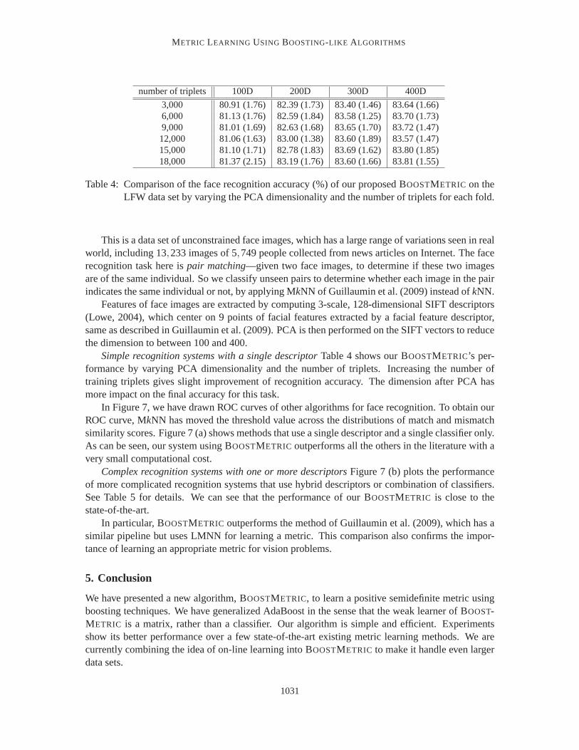
number of triplets 100D 200D 300D 400D

3,000 80.91 (1.76) 82.39 (1.73) 83.40 (1.46) 83.64 (1.66)6,000 81.13 (1.76) 82.59 (1.84) 83.58 (1.25) 83.70 (1.73)9,000 81.01 (1.69) 82.63 (1.68) 83.65 (1.70) 83.72 (1.47)12,000 81.06 (1.63) 83.00 (1.38) 83.60 (1.89) 83.57 (1.47)15,000 81.10 (1.71) 82.78 (1.83) 83.69 (1.62) 83.80 (1.85)18,000 81.37 (2.15) 83.19 (1.76) 83.60 (1.66) 83.81 (1.55)

Table 4: Comparison of the face recognition accuracy (%) of our proposed BOOSTMETRIC on theLFW data set by varying the PCA dimensionality and the number of triplets for each fold.

This is a data set of unconstrained face images, which has a large range of variations seen in realworld, including 13,233 images of 5,749 people collected from news articles on Internet. The facerecognition task here ispair matching—given two face images, to determine if these two imagesare of the same individual. So we classify unseen pairs to determine whethereach image in the pairindicates the same individual or not, by applying MkNN of Guillaumin et al. (2009) instead ofkNN.

Features of face images are extracted by computing 3-scale, 128-dimensional SIFT descriptors(Lowe, 2004), which center on 9 points of facial features extracted bya facial feature descriptor,same as described in Guillaumin et al. (2009). PCA is then performed on the SIFT vectors to reducethe dimension to between 100 and 400.

Simple recognition systems with a single descriptorTable 4 shows our BOOSTMETRIC’s per-formance by varying PCA dimensionality and the number of triplets. Increasing the number oftraining triplets gives slight improvement of recognition accuracy. The dimension after PCA hasmore impact on the final accuracy for this task.

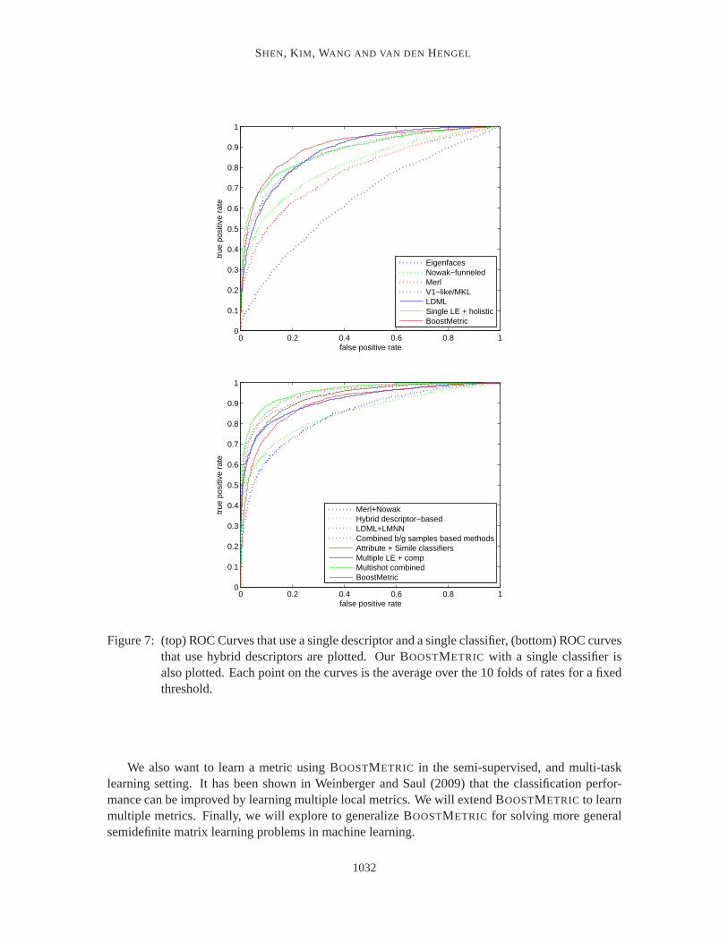
In Figure 7, we have drawn ROC curves of other algorithms for face recognition. To obtain ourROC curve, MkNN has moved the threshold value across the distributions of match and mismatchsimilarity scores. Figure 7 (a) shows methods that use a single descriptor and a single classifier only.As can be seen, our system using BOOSTMETRIC outperforms all the others in the literature with avery small computational cost.

Complex recognition systems with one or more descriptorsFigure 7 (b) plots the performanceof more complicated recognition systems that use hybrid descriptors or combination of classifiers.See Table 5 for details. We can see that the performance of our BOOSTMETRIC is close to thestate-of-the-art.

In particular, BOOSTMETRIC outperforms the method of Guillaumin et al. (2009), which has asimilar pipeline but uses LMNN for learning a metric. This comparison also confirms the impor-tance of learning an appropriate metric for vision problems.

5. Conclusion

We have presented a new algorithm, BOOSTMETRIC, to learn a positive semidefinite metric usingboosting techniques. We have generalized AdaBoost in the sense that theweak learner of BOOST-METRIC is a matrix, rather than a classifier. Our algorithm is simple and efficient. Experimentsshow its better performance over a few state-of-the-art existing metric learning methods. We arecurrently combining the idea of on-line learning into BOOSTMETRIC to make it handle even largerdata sets.

1031


0 0.2 0.4 0.6 0.8 10

0.1

0.2

0.3

0.4

0.5

0.6

0.7

0.8

0.9

1

false positive rate

true

pos

itive

rat

e

EigenfacesNowak−funneledMerlV1−like/MKLLDMLSingle LE + holisticBoostMetric

0 0.2 0.4 0.6 0.8 10

0.1

0.2

0.3

0.4

0.5

0.6

0.7

0.8

0.9

1

false positive rate

true

pos

itive

rat

e

Merl+NowakHybrid descriptor−basedLDML+LMNNCombined b/g samples based methodsAttribute + Simile classifiersMultiple LE + compMultishot combinedBoostMetric

Figure 7: (top) ROC Curves that use a single descriptor and a single classifier, (bottom) ROC curvesthat use hybrid descriptors are plotted. Our BOOSTMETRIC with a single classifier isalso plotted. Each point on the curves is the average over the 10 folds of rates for a fixedthreshold.

We also want to learn a metric using BOOSTMETRIC in the semi-supervised, and multi-tasklearning setting. It has been shown in Weinberger and Saul (2009) thatthe classification perfor-mance can be improved by learning multiple local metrics. We will extend BOOSTMETRIC to learnmultiple metrics. Finally, we will explore to generalize BOOSTMETRIC for solving more generalsemidefinite matrix learning problems in machine learning.

1032


single descriptor + single classifiermultiple descriptors/classifiers

Turk and Pentland (1991) 60.02 (0.79) -‘Eigenfaces’

Nowak and Jurie (2007) 73.93 (0.49) -‘Nowak-funneled’

Huang et al. (2008) 70.52 (0.60) 76.18 (0.58)‘Merl’ ‘Merl+Nowak’

Wolf et al. (2008) - 78.47 (0.51)‘Hybrid descriptor-based’

Wolf et al. (2009) 72.02 86.83 (0.34)- ‘Combined b/g samples based’

Pinto et al. (2009) 79.35 (0.55) -‘V1-like/MKL’

Taigman et al. (2009) 83.20 (0.77) 89.50 (0.40)- ‘Multishot combined’

Kumar et al. (2009) - 85.29 (1.23)‘attribute + simile classifiers’

Cao et al. (2010) 81.22 (0.53) 84.45 (0.46)‘single LE + holistic’ ‘multiple LE + comp’

Guillaumin et al. (2009) 83.2 (0.4) 87.5 (0.4)‘LDML’ ‘LMNN + LDML’

BOOSTMETRIC 83.81 (1.55) -‘B OOSTMETRIC’ on SIFT

Table 5: Test accuracy in percentage (mean and standard deviation) onthe LFW data set. ROCcurve labels in Figure 7 are described here with details.

References

A. Bar-Hillel, T. Hertz, N. Shental, and D. Weinshall. Learning a Mahalanobis metric from equiva-lence constraints.J. Machine Learning Research, 6:937–965, 2005.

O. Boiman, E. Shechtman, and M. Irani. In defense of nearest-neighbor based image classification.In Proc. IEEE Int’l Conf. Computer Vision and Pattern Recognition, 2008.

B. Borchers. CSDP, a C library for semidefinite programming.Optimization Methods and Software,11(1):613–623, 1999.

S. Boyd and L. Vandenberghe.Convex Optimization. Cambridge University Press, 2004.

Z. Cao, Q. Yin, X. Tang, and J. Sun. Face recognition with learning-based descriptor. InProc. IEEEInt’l Conf. Computer Vision and Pattern Recognition, 2010.

G. B. Dantzig and P. Wolfe. Decomposition principle for linear programs.Operation Research, 8(1):101–111, 1960.

J. V. Davis, B. Kulis, P. Jain, S. Sra, and I. S. Dhillon. Information-theoretic metric learning. InInt’l Conf. Machine Learning, pages 209–216, Corvalis, Oregon, 2007. ACM Press.

1033


A. Demiriz, K.P. Bennett, and J. Shawe-Taylor. Linear programming boosting via column genera-tion. Machine Learning, 46(1-3):225–254, 2002.

P. Drineas, R. Kannan, and M. Mahoney. Fast Monte Carlo algorithms for matrices II: Computinga compressed approximate matrix decomposition.SIAM J. Computing, 36:2006, 2004.

L. Fei-Fei, R. Fergus, and P. Perona. One-shot learning of object categories.IEEE Trans. PatternAnalysis and Machine Intelligence, 28(4):594–611, April 2006.

P. A. Fillmore and J. P. Williams. Some convexity theorems for matrices.Glasgow Math. Journal,12:110–117, 1971.

A. Frome, Y. Singer, F. Sha, and J. Malik. Learning globally-consistentlocal distance functions forshape-based image retrieval and classification. InProc. IEEE Int’l Conf. Computer Vision, 2007.

A. Globerson and S. Roweis. Metric learning by collapsing classes. InProc. Advances in NeuralInformation Processing Systems, 2005.

J. Goldberger, S. Roweis, G. Hinton, and R. Salakhutdinov. Neighbourhood component analysis.In Proc. Advances in Neural Information Processing Systems. MIT Press, 2004.

M. Guillaumin, J. Verbeek, and C. Schmid. Is that you? metric learning approaches for face identi-fication. InProc. IEEE Int’l Conf. Computer Vision, 2009.

T. Hastie and R. Tibshirani. Discriminant adaptive nearest neighbor classification. IEEE Trans.Pattern Analysis and Machine Intelligence, 18(6):607–616, 1996.

X. He, S. Yan, Y. Hu, P. Niyogi, and H.-J. Zhang. Face recognition using Laplacianfaces.IEEETrans. Pattern Analysis and Machine Intelligence, 27(3):328–340, 2005.

G. B. Huang, M. Ramesh, T. Berg, and E. Learned-Miller. Labeled faces in the wild: A databasefor studying face recognition in unconstrained environments. TechnicalReport 07-49, Universityof Massachusetts, Amherst, October 2007.

G. B. Huang, M. J. Jones, and E. Learned-Miller. LFW results using a combined nowak plus merlrecognizer. InFaces in Real-Life Images Workshop in Euro. Conf. Computer Vision, 2008.

B. Jian and B. C. Vemuri. Metric learning using Iwasawa decomposition. InProc. IEEE Int’l Conf.Computer Vision, Rio de Janeiro, Brazil, 2007. IEEE.

M. Krein and D. Milman. On extreme points of regular convex sets.Studia Mathematica, 9:133–138, 1940.

N. Kumar, A. C. Berg, P. N. Belhumeur, and S. K. Nayar. Attribute and simileclassifiers for faceverification. InProc. IEEE Int’l Conf. Computer Vision, 2009.

D. G. Lowe. Distinctive image features from scale-invariant keypoints.Int’l J. Computer Vision, 60(2):91–110, 2004.

M. E. Lubbecke and J. Desrosiers. Selected topics in column generation.Operation Research, 53(6):1007–1023, 2005.

1034


K. Mikolajczyk and C. Schmid. Scale & affine invariant interest point detectors. Int’l J. ComputerVision, 60(1):63–86, 2004.

E. Nowak and F. Jurie. Learning visual similarity measures for comparing never seen objects. InProc. IEEE Int’l Conf. Computer Vision and Pattern Recognition, 2007.

M. L. Overton and R. S. Womersley. On the sum of the largest eigenvaluesof a symmetric matrix.SIAM J. Matrix Analysis and Application, 13(1):41–45, 1992.

N. Pinto, J. J. DiCarlo, and D. D. Cox. How far can you get with a modern face recognition test setusing only simple features? InProc. IEEE Int’l Conf. Computer Vision and Pattern Recognition,2009.

R. Rosales and G. Fung. Learning sparse metrics via linear programming. InProc. ACM SIGKDDInt’l Conf. Knowledge discovery and Data Mining, pages 367–373. ACM, 2006.

S. Rosset, J. Zhu, and T. Hastie. Boosting as a regularized path to a maximummargin classifier.J.Machine Learning Research, 5:941–973, 2004.

R. E. Schapire. Theoretical views of boosting and applications. InProc. Int’l Conf. AlgorithmicLearning Theory, pages 13–25, London, UK, 1999. Springer-Verlag.

M. Schultz and T. Joachims. Learning a distance metric from relative comparisons. InProc. Ad-vances in Neural Information Processing Systems. MIT Press, 2003.

C. Shen and H. Li. On the dual formulation of boosting algorithms.IEEE Trans. Pattern Analysisand Machine Intelligence, 32(12):2216–2231, 2010.

C. Shen, A. Welsh, and L. Wang. PSDBoost: Matrix-generation linear programming for positivesemidefinite matrices learning. In D. Koller, D. Schuurmans, Y. Bengio, andL. Bottou, editors,Proc. Advances in Neural Information Processing Systems, pages 1473–1480, Vancouver, B.C.,Canada, December 2008. MIT Press.

C. Shen, J. Kim, L. Wang, and A. van den Hengel. Positive semidefinite metriclearning with boost-ing. In Y. Bengio, D. Schuurmans, J. Lafferty, C. Williams, and A. Culotta,editors,Proc. Ad-vances in Neural Information Processing Systems, pages 1651–1659, Vancouver, B.C., Canada,December 2009. MIT Press.

Y. Taigman, L. Wolf, and T. Hassner. Multiple one-shots for utilizing class label information. InProc. British Machine Vision Conf., 2009.

K. Tsuda, G. Ratsch, and M. K. Warmuth. Matrix exponentiated gradient updates for on-line learn-ing and Bregman projection.J. Machine Learning Research, 6:995–1018, December 2005.

M. A. Turk and A. P. Pentland. Face recognition using eigenfaces. InProc. IEEE Int’l Conf.Computer Vision and Pattern Recognition, 1991.

H. Wang, H. Huang, and C. Ding. Discriminant Laplacian embedding. InProc. AAAI Conf. ArtificialIntelligence, pages 618–623, 2010a.

1035


S. Wang and R. Jin. An information geometry approach for distance metric learning. InProc. Int’lConf. Artificial Intelligence and Statistics, pages 591–598, 2009.

Z. Wang, Y. Hu, and L.-T. Chia. Image-to-class distance metric learning for image classification.In Proc. Euro. Conf. Computer Vision, volume Lecture Notes in Computer Science 6311/2010,pages 706–719, 2010b.

M. K. Warmuth, J. Liao, and G. Ratsch. Totally corrective boosting algorithms that maximize themargin. InInt’l Conf. Machine Learning, pages 1001–1008, Pittsburgh, Pennsylvania, 2006.

K. Q. Weinberger and L. K. Saul. Unsupervised learning of image manifolds by semidefinite pro-gramming.Int’l J. Computer Vision, 70(1):77–90, 2006.

K. Q. Weinberger and L. K. Saul. Distance metric learning for large margin nearest neighbor clas-sification.J. Machine Learning Research, 10:207–244, 2009.

K. Q. Weinberger, J. Blitzer, and L. K. Saul. Distance metric learning for large margin nearestneighbor classification. InProc. Advances in Neural Information Processing Systems, pages1473–1480, 2005.

J. Winn, A. Criminisi, and T. Minka. Object categorization by learned universal visual dictionary.In Proc. IEEE Int’l Conf. Computer Vision, pages 1800–1807, 2005.

L. Wolf, T. Hassner, and Y. Taigman. Descriptor based methods in the wild.In Faces in Real-LifeImages Workshop in Euro. Conf. Computer Vision, 2008.

L. Wolf, T. Hassner, and Y. Taigman. Similarity scores based on background samples. InProc.Asian Conf. Computer Vision, 2009.

E. Xing, A. Ng, M. Jordan, and S. Russell. Distance metric learning, with application to clusteringwith side-information. InProc. Advances in Neural Information Processing Systems. MIT Press,2002.

J. Yu, J. Amores, N. Sebe, P. Radeva, and Q. Tian. Distance learning for similarity estimation.IEEETrans. Pattern Analysis and Machine Intelligence, 30(3):451–462, 2008.

T. Zhang. Sequential greedy approximation for certain convex optimizationproblems.IEEE Trans.Information Theory, 49(3):682–691, 2003.

C. Zhu, R. H. Byrd, and J. Nocedal. L-BFGS-B: Algorithm 778: L-BFGS-B, FORTRAN routinesfor large scale bound constrained optimization.ACM Trans. Mathematical Software, 23(4):550–560, 1997.

1036

Documents

Positive Semidefinite Metric Learning Using Boosting-like Algorithms