Embed Size (px)
Citation preview
Commun Nonlinear Sci Numer Simulat 15 (2010) 690–699
Contents lists available at ScienceDirect
Commun Nonlinear Sci Numer Simulat
journal homepage: www.elsevier .com/locate /cnsns
Positive solutions of nonlinear m-point BVP for an increasinghomeomorphism and positive homomorphism with sign changingnonlinearity on time scales q
Wei Han a,b,*, Zhen Jin a
a Department of Mathematics, North University of China, Taiyuan, Shanxi 030051, PR Chinab School of Mathematical Sciences, Fudan University, Shanghai 200433, PR China
a r t i c l e i n f o
Article history:Received 13 November 2008Received in revised form 14 April 2009Accepted 14 April 2009Available online 23 April 2009
PACS:02.30.Hq02.30.Sa02.30.Rz
Keywords:Time scalePositive solutionsBoundary value problemFixed point theoremsIncreasing homeomorphism and positivehomomorphism
1007-5704/$ - see front matter � 2009 Elsevier B.Vdoi:10.1016/j.cnsns.2009.04.012
q Project supported by the National Natural SciencUniversity (NCET050271), and the Special Scientific
* Corresponding author. Address: Department ofE-mail address: [email protected] (W. H
a b s t r a c t
In this paper, by using fixed point theorems in cones, some new existence criteria for posi-tive solutions of the nonlinear m-point boundary value problem with an increasing homeo-morphism and positive homomorphism are presented. The nonlinear term f is allowed tochange sign. In particular, our criteria generalize and improve some known results [20] andthe obtained conditions are different from related literature [16,17,23]. As an application,one representative example to demonstrate our results are given.
� 2009 Elsevier B.V. All rights reserved.
1. Introduction
The theory of time scales, which has recently received a lot of attention, was introduced by Stefan Hilger in his PhD thesisin 1988 (supervised by Bernd Aulbach) in order to unify continuous and discrete analysis, see [7]. The time scales calculushas a tremendous potential for applications. For example, it can model insect populations that are continuous while in sea-son (and may follow a difference scheme with variable step-size), die out in (say) winter, while their eggs are incubating ordormant, and then hatch in a new season, giving rise to a nonoverlapping population, see [7].
For the convenience of statements, now we present some basic definitions which can be found in [1,5,7,8]. The book [7] isan excellent source on Dynamic Equations on Time Scales.
A time scale T is a nonempty closed subset of R. We make the blanket assumption that 0, T are points in T. By an interval(0, T), we always mean the intersection of the real interval (0, T) with the given time scale, that is ð0; TÞ \ T, see [7].
. All rights reserved.
e Foundation of China under Grant No. 60771026, the Programme for New Century Excellent Talents inResearch Foundation for the Subjects of Doctors in University (20060110005).
Mathematics, North University of China, Taiyuan, Shanxi 030051, PR China.an).
W. Han, Z. Jin / Commun Nonlinear Sci Numer Simulat 15 (2010) 690–699 691
Definition 1.1. A time scale T is a nonempty closed subset of real numbers R. For t sup T and r > inf T, define the forwardjump operator r and backward jump operator q, respectively, by
rðtÞ ¼ inffs 2 T j s > tg 2 T; qðrÞ ¼ supfs 2 T j s < rg 2 T:
for all t; r 2 T. If rðtÞ > t, t is said to be right scattered, and if qðrÞ < r, r is said to be left scattered; if rðtÞ ¼ t, t is said to beright dense, and if qðrÞ ¼ r, r is said to be left dense. If T has a right scattered minimum m, define Tk ¼ T� fmg; otherwise setTk ¼ T. If T has a left scattered maximum M, define Tk ¼ T� fMg; otherwise set Tk ¼ T.
Definition 1.2. For f : T! R and t 2 Tk, the delta derivative of f at the point t is defined to be the number f MðtÞ, (provided itexists), with the property that for each � > 0, there is a neighborhood U of t such that
jf ðrðtÞÞ � f ðsÞ � f MðtÞðrðtÞ � sÞj 6 �jrðtÞ � sj;
for all s 2 U.For f : T! R and t 2 Tk, the nabla derivative of f at t is the number f5ðtÞ, (provided it exists), with the property that for
each � > 0, there is a neighborhood U of t such that
jf ðqðtÞÞ � f ðsÞ � f5ðtÞðqðtÞ � sÞj 6 �jqðtÞ � sj;
for all s 2 U.
Definition 1.3. A function f is left-dense continuous (i.e. ld-continuous), if f is continuous at each left-dense point in T and itsright-sided limit exists (finite) at each right-dense point in T. The set of left-dense continuous functions f will be denoted byCldðTÞ. f 2 Cldðð0; TÞ; ½0;þ1ÞÞ denotes that f maps ð0; TÞ into ½0;þ1Þ and is ld-continuous.
Definition 1.4. If GMðtÞ ¼ f ðtÞ, then we define the delta integral by
Z baf ðtÞMt ¼ GðbÞ � GðaÞ:
If F5ðtÞ ¼ f ðtÞ, then we define the nabla integral by
Z baf ðtÞ 5 t ¼ FðbÞ � FðaÞ:
In this paper, we will be concerned with the existence of positive solutions for the following dynamic equations on timescales:
M 5
ð/ðu ÞÞ þ aðtÞf ðt;uðtÞÞ ¼ 0; t 2 ð0; TÞ; ð1:1Þuð0Þ ¼Xm�2
i¼1
aiuðniÞ; /ðuMðTÞÞ ¼Xm�2
i¼1
bi/ðuMðniÞÞ; ð1:2Þ
where / : R! R is an increasing homeomorphism and positive homomorphism and /ð0Þ ¼ 0.A projection / : R! R is called an increasing homeomorphism and positive homomorphism, if the following conditions
are satisfied:
(i) if x 6 y, then /ðxÞ 6 /ðyÞ; 8x; y 2 R;(ii) / is a continuous bijection and its inverse mapping is also continuous;
(iii) /ðxyÞ ¼ /ðxÞ/ðyÞ; 8x; y 2 Rþ ¼ ½0;þ1Þ.
We will assume that the following conditions are satisfied throughout this paper:
ðH1Þ 0 < n1 < � � � < nm�2 < qðTÞ; ai; bi 2 ½0;þ1Þ satisfy 0 <Pm�2
i¼1 ai < 1, andPm�2
i¼1 bi < 1;
ðH2Þ aðtÞ 2 Cldðð0; TÞ; ½0;þ1ÞÞ and there exists t0 2 ðnm�2; TÞ, such that aðt0Þ > 0;
ðH3Þ f 2 Cð½0; T� � ½0;þ1Þ; ð�1;þ1ÞÞ; f ðt;0ÞP 0 and f ðt;0Þ–0.
Recently, there has been much attention paid to the existence of positive solutions for second-order nonlinear boundaryvalue problems on time scales, for examples, see [3,9,14,25,26] and references therein. At the same time, multipoint nonlin-ear boundary value problems with p-Laplacian operators on time scales have also been studied extensively in the literature,for details, see [4,12,13,18,21–24] and references therein. But to the best of our knowledge, few people considered the sec-ond-order dynamic equations of increasing homeomorphism and positive homomorphism on time scales.
692 W. Han, Z. Jin / Commun Nonlinear Sci Numer Simulat 15 (2010) 690–699
For the existence problems of positive solutions of boundary value problems on time scales, some authors have obtainedmany results in the recent years, see [4,10,12,13,19,24] and the references therein. However, the key conditions used in theabove papers is that the nonlinearity is nonnegative, so the solution is concave down. If the nonlinear term is negative some-where, then the solution needs no longer be concave down. As a result, it is difficult to find positive solutions of the p-Lapla-cian equation when the nonlinearity change sign.
The present work is moviated by recent papers [16,17,23]. In [17], Liu and Zhang considered the following quasilineardifferential equation
ðuðx0ÞÞ0 þ aðtÞf ðxðtÞÞ ¼ 0; t 2 ð0;1Þ; ð1:3Þxð0Þ � bx0ð0Þ ¼ 0; xð1Þ þ dx0ð1Þ ¼ 0; ð1:4Þ
where u : R! R is an increasing homeomorphism and homomorphism and uð0Þ ¼ 0. By a simple application of a fixed pointindex theorem in cones, they obtained the existence of positive solutions of the problem (1.3) and (1.4). They defined thecompletely continuous operator T as follows:
ðTxÞðtÞ ¼bu�1
R s0 aðsÞf ðxðsÞÞds
� �þR t
0 u�1R s
s aðsÞf ðxðs1ÞÞds1� �
ds; 0 6 t 6 s;
du�1R 1s aðsÞf ðxðsÞÞds
� �þR 1
t u�1R ss aðsÞf ðxðs1ÞÞds1
� �ds; s 6 t 6 1:
8<: ð1:5Þ
But the fixed points of T are not always solutions of Eqs. (1.3) and (1.4) (for example s 6 t 6 1). Since
uð�ðTxÞ0ðtÞÞ–�uððTxÞ0ðtÞÞ:
In [16], Liang and Zhang studied the existence of countably many positive solutions for nonlinear singular boundary valueproblems:
ðuðu0ÞÞ0 þ aðtÞf ðuðtÞÞ ¼ 0; t 2 ð0;1Þ; ð1:6Þ
uð0Þ ¼Xm�2
i¼1
aiuðniÞ; uðu0ð1ÞÞ ¼Xm�2
i¼1
biuðu0ðniÞÞ; ð1:7Þ
where u : R! R is an increasing homeomorphism and positive homomorphism and uð0Þ ¼ 0. By using the fixed point indextheory and a new fixed-point theorem in cones, they obtained countably many positive solutions for the problem (1.6) and(1.7).
Su et al. [23] investigated the following singular m-point p-Laplacian boundary value problem on time scales with thesign changing nonlinearity:
ðupðuMðtÞÞÞ5 þ aðtÞf ðt;uðtÞÞ ¼ 0; t 2 ð0; TÞ; ð1:8Þ
uð0Þ ¼ 0; uðTÞ �Xm�2
i¼1
wiðuðniÞÞ ¼ 0; ð1:9Þ
where upðuÞ ¼ jujp�2u; p > 1, 0 < n1 < � � � < nm�2 < qðTÞ; aðtÞ 2 Cldðð0; TÞ; ð0;þ1ÞÞ; f 2 Cldðð0; TÞ � ð0;þ1Þ; ð�1;þ1ÞÞ. They
presented some new existence criteria for positive solutions of the problem (1.8) and (1.9) by using the well-known Schau-der fixed point theorem and upper and lower solutions method.
To date no paper has appeared in the literature which discusses the multipoint boundary value problem for increasinghomeomorphism and positive homomorphism on time scales when nonlinear term may change sign. In this paper, onthe one hand, our work concentrates on the case when the nonlinear term may change sign, we will use the property ofthe solutions of the BVP (1.1) and (1.2) to overcome the difficulty. On the other hand, we will establish the key conditionsin Theorems 3.1 and 3.2 to show the existence of positive solutions of the BVP (1.1) and (1.2).
The rest of the paper is arranged as follows. We state some basic time scale definitions and prove several preliminaryresults in Sections 2 and 3 is devoted to the existence of positive solution of (1.1) and (1.2), the main tool being the fixedpoint theorem in cone. At the end of the paper, we will give a representative example which illustrate that our work is true.We also point out that when T ¼ R; p ¼ 2, (1.1) and (1.2) becomes a boundary value problem of differential equations andjust is the problem considered in [20]. Our main results extend and include the main results of [16,17,20,27].
2. Some useful lemmas
To prove the main results in this paper, we will employ several lemmas. These lemmas are based on the linear BVP
ð/ðuMÞÞ5 þ hðtÞ ¼ 0; t 2 ð0; TÞ; ð2:1Þ
uð0Þ ¼Xm�2
i¼1
aiuðniÞ; /ðuMðTÞÞ ¼Xm�2
i¼1
bi/ðuMðniÞÞ: ð2:2Þ
W. Han, Z. Jin / Commun Nonlinear Sci Numer Simulat 15 (2010) 690–699 693
Lemma 2.1. IfPm�2
i¼1 ai–1 andPm�2
i¼1 bi–1, then for h 2 Cld½0; T� the BVP (2.1) and (2.2) has the unique solution
uðtÞ ¼Z t
0/�1
Z T
shðsÞ 5 s� A
� �Msþ B; ð2:3Þ
where
A ¼ �
Pm�2
i¼1biR T
nihðsÞ 5 s
1�Pm�2
i¼1bi
; B ¼
Pm�2
i¼1aiR ni
0 /�1 R Ts hðsÞ 5 s� A
� �Ms
1�Pm�2
i¼1ai
:
Proof. Let u be as in (2.3). By, [5, Theorem 2.10(iii)], taking the delta derivative of (2.3), we have
uMðtÞ ¼ /�1Z T
thðsÞ 5 s� A
� �;
moreover, we get
/ðuMÞ ¼Z T
thðsÞ 5 s� A;
taking the nabla derivative of this expression yields ð/ðuMÞÞ5 ¼ �hðtÞ. And routine calculation verify that u satisfies theboundary value conditions in (2.2), so that u given in (2.3) is a solution of (2.1) and (2.2).
It is easy to see that BVP ð/ðuMÞÞ5 ¼ 0; uð0Þ ¼Pm�2
i¼1 aiuðniÞ; /ðuMðTÞÞ ¼Pm�2
i¼1 bi/ðuMðniÞÞ has only the trivial solution.Thus u in (2.3) is the unique solution of (2.1) and (2.2). h
Lemma 2.2. Assume ðH1Þ holds, For h 2 Cld½0; T� and h P 0, then the unique solution u of (2.1) and 2.2) satisfies
uðtÞP 0; for t 2 ½0; T�:
Proof. Let
w0ðsÞ ¼ /�1Z T
shðsÞ 5 s� A
� �:
Since
Z TshðsÞ 5 s� A ¼
Z T
shðsÞ 5 sþ
Pm�2i¼1 bi
R Tni
hðsÞ 5 s
1�Pm�2
i¼1 bi
P 0;
then w0ðsÞP 0.So we can easily get uðtÞP 0; t 2 ½0; T�. h
Lemma 2.3. Assume ðH1Þ holds, if h 2 Cld½0; T� and h P 0, then the unique solution u of (2.1) and (2.2) satisfies
inft2½0;T�
uðtÞP ckuk;
where
c ¼Pm�2
i¼1 aini
1�Pm�2
i¼1 ai
� �T þ
Pm�2i¼1 aini
; kuk ¼ maxt2½0;T�
juðtÞj:
Proof. It is easy to check that uMðtÞ ¼ w0ðtÞP 0, this implies that
kuk ¼ uðTÞ; mint2½0;T�
uðtÞ ¼ uð0Þ:
It is easy to see that uMðt2Þ 6 uMðt1Þ for any t1; t2 2 ½0; T� with t1 6 t2. Hence uMðtÞ is a decreasing function on ½0; T�. Thismeans that the graph of uðtÞ is concave down on ð0; TÞ.
For each i 2 f1;2; � � � ;m� 2g, we have
uðTÞ � uð0ÞT � 0
PuðTÞ � uðniÞ
T � ni;
i.e.,
TuðniÞ � niuðTÞP ðT � niÞuð0Þ;
694 W. Han, Z. Jin / Commun Nonlinear Sci Numer Simulat 15 (2010) 690–699
so that
Tsumm�2i¼1 aiuðniÞ �
Xm�2
i¼1
ainiuðTÞPXm�2
i¼1
aiðT � niÞuð0Þ:
With the boundary condition uð0Þ ¼Pm�2
i¼1 aiuðniÞ, we have
uð0ÞPPm�2
i¼1 aini
T �Pm�2
i¼1 aiðT � niÞuðTÞ ¼
Pm�2i¼1 aini
1�Pm�2
i¼1 ai
� �T þ
Pm�2i¼1 aini
uðTÞ: �
Let E ¼ Cldð½0; T�;RÞ be the set of all ld-continuous functions from ½0; T� to R, and Let the norm on Cldð½0; T�;RÞ be the max-imum norm. Then the Cldð½0; T�;RÞ is a Banach space. We define three cones by
P ¼ fu : u 2 E; uðtÞP 0; t 2 ½0; T�g;P0 ¼ fu : u 2 E; uðtÞ is concave; nonnegative and increasing on ½0; T�g;
and
K ¼ fuju 2 E;uðtÞis nonnegative and increasing on½0; T�; inft2½0;T�
uðtÞP ckukg;
where c is the same as in Lemma 2.3.It is easy to see that the BVP (1.1) and (1.2) has a solution u ¼ uðtÞ if and only if u solves the equation
uðtÞ ¼Z t
0/�1
Z T
saðsÞf ðs; uðsÞÞ 5 s� ~A
� �Msþ ~B;
where
eA ¼ �Pm�2i¼1 bi
R Tni
aðsÞf ðs; uðsÞÞ 5 s
1�Pm�2
i¼1 bi
;
eB ¼Pm�2i¼1 ai
R ni0 /�1 R T
s aðsÞf ðs; uðsÞÞ 5 s� eA� �Ms
1�Pm�2
i¼1 ai
:
We define the operators G : P ! E and H : K ! E as follows:
ðGuÞðtÞ ¼Z t
0/�1
Z T
saðsÞf ðs;uðsÞÞ 5 s� eA� �
Msþ eB; ð2:4Þ
ðHuÞðtÞ ¼Z t
0/�1
Z T
saðsÞfþðs;uðsÞÞ 5 s� bA� �
Msþ bB; ð2:5Þ
where eA; eB are given in the above expressions, and
bA ¼ �Pm�2i¼1 bi
R Tni
aðsÞfþðs;uðsÞÞ 5 s
1�Pm�2
i¼1 bi
;
bB ¼Pm�2i¼1 ai
R ni0 /�1 R T
s aðsÞfþðs;uðsÞÞ 5 s� bA� �Ms
1�Pm�2
i¼1 ai
;
fþðt;uðtÞÞ ¼maxff ðt; uðtÞÞ; 0g; t 2 ½0; T�:
It is obvious that K is a cone in E. By Lemma 2.3, HðKÞ � K . So by applying Arzela–Ascoli theorem on time scales [2], wecan obtain that HðKÞ is relatively compact. In view of Lebesgue’s dominated convergence theorem on time scales [6], it iseasy to prove that H is continuous. Hence, H : K ! K is completely continuous.
Lemma 2.4 (see [11]). Let K be a cone in a Banach space X. Let D be an open bounded subset of X with DK ¼ D \ K–/ and DK –K.Assume that A : DK ! K is a completely continuous map such that x–Ax for x 2 @DK . Then the following results hold:
(1) If kAxk 6 kxk; x 2 @DK , then iðA;DK ;KÞ ¼ 1;(2) If there exists x0 2 K n fhg such that x–Axþ kx0, for all x 2 @DK and all k > 0, then iðA;DK ;KÞ ¼ 0;(3) Let UK be open in X such that UK � DK . If iðA;DK ;KÞ ¼ 1 and iðA;UK ;KÞ ¼ 0, then A has a fixed point in DK n UK .
The same results holds, if iðA;DK ;KÞ ¼ 0 and iðA;UK ;KÞ ¼ 1.We define
Kq ¼ fuðtÞ 2 K : kuk < qg; Xq ¼ fuðtÞ 2 K : min06t6T
uðtÞ < cqg:
W. Han, Z. Jin / Commun Nonlinear Sci Numer Simulat 15 (2010) 690–699 695
Lemma 2.5 (see [15]). Xq defined above has the following properties:
(a) Kcq � Xq � Kq;
(b) Xq is open relative to K;(c) x 2 @Xq if and only if min06t6T xðtÞ ¼ cq;(d) If x 2 @Xq, then cq 6 xðtÞ 6 q for t 2 ½0; T�.
Now, for the convenience, we introduce the following notations. Let
uðsÞ ¼ /�1Z T
saðsÞfþðs; uðsÞÞ 5 s� bA� �
;
f qcq ¼min min
06t6T
f ðt;uÞ/ðqÞ : u 2 ½cq;q�
� ;
f q0 ¼max max
06t6T
f ðt; uÞ/ðqÞ : u 2 ½0;q�
� ;
f a ¼ limu!a
sup max06t6T
f ðt; uÞ/ðuÞ ; f a ¼ lim
u!ainf min
06t6T
f ðt;uÞ/ðuÞ ; ða :¼ 1 or 0þÞ;
m ¼Z T
0/�1
Z T
saðsÞ 5 sþ
Pm�2i¼1 bi
R Tni
aðsÞ 5 s
1�Pm�2
i¼1 bi
" #Msþ
Pm�2i¼1 ai
1�Pm�2
i¼1 ai
Z ni
0/�1
Z T
saðsÞ 5 sþ
Pm�2i¼1 bi
R Tni
aðsÞ 5 s
1�Pm�2
i¼1 bi
" #Ms
( )�1
;
ð2:6Þ
M ¼Pm�2
i¼1 ai
1�Pm�2
i¼1 ai
Z ni
0/�1
Z T
saðsÞ 5 sþ
Pm�2i¼1 bi
R Tni
aðsÞ 5 s
1�Pm�2
i¼1 bi
" #Ms
( )�1
: ð2:7Þ
Lemma 2.6. If f satisfies the following conditions
f q0 6 /ðmÞ and u–Hu; for u 2 @ Kq; ð2:8Þ
then iðH;Kq;KÞ ¼ 1.
Proof. By (2.6) and (2.8), we have for 8u 2 @ Kq,
Z TsaðsÞfþðs;uðsÞÞ 5 s� bA ¼ Z T
saðsÞfþðs;uðsÞÞ 5 sþ
Pm�2i¼1 bi
R Tni
aðsÞfþðs;uðsÞÞ 5 s
1�Pm�2
i¼1 bi
6 /ðqÞ/ðmÞZ T
saðsÞ 5 sþ
Pm�2i¼1 bi
R Tni
aðsÞ 5 s
1�Pm�2
i¼1 bi
" #;
so that
uðsÞ ¼ /�1Z T
saðsÞfþðs;uðsÞÞ 5 s� bA� �
6 qm/�1Z T
saðsÞ 5 sþ
Pm�2i¼1 bi
R Tni
aðsÞ 5 s
1�Pm�2
i¼1 bi
" #:
Therefore, by (2.6), we have
kHuk 6Z T
0uðsÞMsþ bB ¼ Z T
0uðsÞMsþ
Pm�2i¼1 ai
R ni0 uðsÞMs
1�Pm�2
i¼1 ai
6 qmZ T
0/�1
Z T
saðsÞ 5 sþ
Pm�2i¼1 bi
R Tni
aðsÞ 5 s
1�Pm�2
i¼1 bi
" #Ms
(
þPm�2
i¼1 ai
1�Pm�2
i¼1 ai
Z ni
0/�1
Z T
saðsÞ 5 sþ
Pm�2i¼1 bi
R Tni
aðsÞ 5 s
1�Pm�2
i¼1 bi
" #Ms
)¼ q ¼ kuk:
This implies that kHuk 6 kuk for u 2 @ Kq. By Lemma 2.4(1), we have
iðH;Kq;KÞ ¼ 1: �
Lemma 2.7. If f satisfies the following conditions
696 W. Han, Z. Jin / Commun Nonlinear Sci Numer Simulat 15 (2010) 690–699
f qcq P /ðMcÞ and u–Hu for u 2 @Xq; ð2:9Þ
then iðH;Xq;KÞ ¼ 0.
Proof. Let eðtÞ � 1, for t 2 ½0; T�; then e 2 @ K1. We claim that u–Huþ ke for u 2 @ Xq, and k > 0. In fact, if not, there existu0 2 @Xq, and k0 > 0 such that u0 ¼ Hu0 þ k0e.
By (2.7) and (2.9), we have for t 2 ½0; T�,
Z T
saðsÞf ðs; u0ðsÞÞ 5 s� bA ¼ Z T
saðsÞfþðs;u0ðsÞÞ 5 sþ
Pm�2i¼1 bi
R Tni
aðsÞfþðs;u0ðsÞÞ 5 s
1�Pm�2
i¼1 bi
P /ðqÞ/ðMcÞZ T
saðsÞ 5 sþ
Pm�2i¼1 bi
R Tni
aðsÞ 5 s
1�Pm�2
i¼1 bi
" #;
so that
uðsÞ ¼ /�1Z T
saðsÞfþðs;u0ðsÞÞ 5 s� eA� �
P qMc/�1Z T
saðsÞ 5 sþ
Pm�2i¼1 bi
R Tni
aðsÞ 5 s
1�Pm�2
i¼1 bi
" #:
Applying (2.7), it follows that
u0ðtÞ ¼ Hu0ðtÞ þ k0eðtÞP bB þ k0 ¼Pm�2
i¼1 aiR ni
0 uðsÞMs
1�Pm�2
i¼1 ai
þ k0
P cqMPm�2
i¼1 ai
1�Pm�2
i¼1 ai
Z ni
0/�1
Z T
saðsÞ 5 sþ
Pm�2i¼1 bi
R Tni
aðsÞ 5 s
1�Pm�2
i¼1 bi
" #Msþ k0 ¼ cqþ k0:
This implies that cq P cqþ k0, a contradiction. Hence, by Lemma 2.4 (2), it follows that
iðH;Xq;KÞ ¼ 0: �
3. Existence theorems of positive solutions
Theorem 3.1. Assume ðH1Þ; ðH2Þ and ðH3Þ hold, and assume that one of the following conditions hold:ðH4Þ There exist q1;q2 2 ð0;þ1Þ with q1 < cq2 such that
ð1Þ f ðt; uÞP 0; t 2 ½0; T�; u 2 ½cq1;q2�;ð2Þ f q1
0 6 /ðmÞ; f q2cq2
P /ðMcÞ;
ðH5Þ There exist q1;q2 2 ð0;þ1Þ with q1 < q2 such that
ð3Þ f q20 6 /ðmÞ:
ð4Þ f ðt; uÞP /ðMcq1Þ; t 2 ½0; T�; u 2 ½c2q1;q2�:
Then (1.1) and (1.2) has a positive solution.
Proof. Assume that ðH4Þ holds. We show that H has a fixed point u1 in Xq2n Kq1
. By Lemma 2.6, we have that
iðH;Kq1;KÞ ¼ 1:
By Lemma 2.7, we have that
iðH;Kq2;KÞ ¼ 0:
By Lemma 2.5 (a) and q1 < cq2, we have Kq1� Kcq2
� Xq2. It follows from Lemma 2.4(3) that A has a fixed point u1 in
Xq2n Kq1
, The proof is similar when H5 holds, and we omit it here. The proof is complete. h
Theorem 3.2. Assume ðH1Þ; ðH2Þ and ðH3Þ hold, and suppose that one of the following conditions holds:ðH8Þ There existq1;q2;q3 2 ð0;þ1Þ with q1 < cq2 and q2 < q3 such that
ð1Þ f q10 6 /ðmÞ; f q2
cq2P /ðMcÞ;u–Hu;8 u 2 @Xq2
; and f q30 6 /ðmÞ;
ð2Þ f ðt; uÞP 0; t 2 ½0; T�; u 2 ½cq1;q3�:
ðH9Þ There exist q1;q2;q3 2 ð0;þ1Þ with q1 < q2 < cq3 such that
W. Han, Z. Jin / Commun Nonlinear Sci Numer Simulat 15 (2010) 690–699 697
ð1Þ f q20 6 /ðmÞ; f q1
cq1P /ðMcÞ; u–Hu;8 u 2 @Kq2
; and f q3cq3
P /ðMcÞ;ð2Þ f ðt; uÞP 0; t 2 ½0; T�; u 2 ½cq2;q3�; and f ðt;uÞP /ðMcq1Þ; t 2 ½0; T�; u 2 ½c2q1;q2�:
Then (1.1), (1.2) has two positive solutions. Moreover, if ðH8Þf q10 6 /ðmÞ is replaced by f q1
0 < /ðmÞ, then (1.1), (1.2) has a thirdpositive solution u3 2 Kq1
.
Proof. Assume ðH8Þ holds, we show that H has a fixed point u1 either in @Kq1or u1 in Xq2
n Kq1. If u–Hu; u 2 @Kq1
S@Kq3
, byLemmas 2.6 and 2.7, we have
iðH;Kq1;KÞ ¼ 1; iðH;Xq2
;KÞ ¼ 0; iðH;Kq3;KÞ ¼ 1:
By Lemma 2.5(a) and q1 < cq2, we have Kq1� Kcq2
� Xq2. By Lemma 2.4(3), we have H has a fixed point u1 2 Xq2
n Kq1. Sim-
ilarly, H has a fixed point u2 2 Kq3nXq2
. Clearly,
ku1k > q1; mint2½0;T�
u1ðtÞ ¼ u1ð0ÞP cku1k > cq1:
This implies that cq1 6 u1ðtÞ 6 q2; t 2 ½0; T�. By ðH8Þð2Þ, we have f ðt;u1ðtÞÞP 0; t 2 ½0; T�, i.e. fþðt;u1ðtÞÞ ¼ f ðt;u1ðtÞÞ. Hence,we can get Hu1 ¼ Gu1. That means u1 is a fixed point of G. From u2 2 Kq3
nXq2; q2 < q3 and Lemma 2.5(a) we have
Kcq2� Xq2
� Kq3. Obviously, ku2k > cq2. This implies that
mint2½0;T�
u2ðtÞ ¼ u2ð0ÞP cku2k > c2q2:
Therefore,
c2q2 6 u2ðtÞ 6 q3; t 2 ½0; T�:
By q1 < cq2 and ðH8Þð2Þ, we have f ðt;u2ðtÞÞP 0; t 2 ½0; T�, i.e. fþðt;u2ðtÞÞ ¼ f ðt;u2ðtÞÞ. So u2 is another fixed point of G. Thus,we have proved that (1.1) and (1.2) has at least two positive solutions u1 and u2. The proof is similar when ðH9Þ holds and weomit it here. The proof is completed. h
Remark 3.1. If T ¼ R, ð0; TÞ ¼ ð0;1Þ, p ¼ 2. Theorems 3.1 and 3.2 improve Theorem 3.1 in [20].
4. Application
The second-order boundary value problem arises in the study of draining and coating flows. We will present a represen-tative example to explain our results in this section.
Example 4.1. Let T ¼ fð12 Þn : n 2 Ng
Sf1g; T ¼ 1. Consider the following BVP on time scales
ð/ðuMÞÞ5 þ f ðt;uðtÞÞ ¼ 0; t 2 ð0; TÞ; ð4:1Þ
uð0Þ ¼ 14
u13
� �; /ðuMðTÞÞ ¼ 1
2/ uMð1
3Þ
� �; ð4:2Þ
where
/ðuÞ ¼u3; u 6 0;
u2; u > 0;
(
f ðt; uÞ :¼ f ðuÞ ¼
u� 110
� �3; u 2 0; 1
10
�;
5081 u� 1
10
� �2; u 2 1
10 ;1 �
;
12 u; u 2 ½1;2�;
1203 ðu2 � 4uþ 4Þ þ 1; u 2 ½2;20�;
1� 812000 ðu2 � 50uþ 599Þ; u 2 ½20;þ1Þ:
8>>>>>>>>>><>>>>>>>>>>:
It is easy to check that f : ½0;1� � ½0;þ1Þ ! ð�1;þ1Þ is continuous. In this case, aðtÞ � 1; a1 ¼ 14 ; b1 ¼ 12 ; n1 ¼ 1
3, it fol-lows from a direct calculation that
698 W. Han, Z. Jin / Commun Nonlinear Sci Numer Simulat 15 (2010) 690–699
m ¼Z T
0/�1 ðT � sÞ þ b1ðT � n1Þ
1� b1
� Msþ a1
1� a1
Z n1
0/�1 ðT � sÞ þ b1ðT � n1Þ
1� b1
� Ms
� �1
¼Z 1
01� sþ
12 ð1� 1
3Þ1� 1
2
!12
Msþ14
1� 14
Z 13
01� sþ
12 1� 1
3
� �1� 1
2
!12
Ms
24 35�1
¼Z 1
0
53� s
� �12
Msþ 13
Z 13
0
53� s
� �12
Ms
" #�1
� 0:8281;
M ¼ a1
1� a1
Z n1
0/�1 ðT � sÞ þ b1ðT � n1Þ
1� b1
� Ms
� �1
¼14
1� 14
Z 13
0
53� s
� �12
Ms
" #�1
� 7:3523;
c ¼ a1n1
ð1� a1ÞT þ a1n1¼
14 � 1
3
ð1� 14Þ � 1þ 1
4 � 13
¼ 110
:
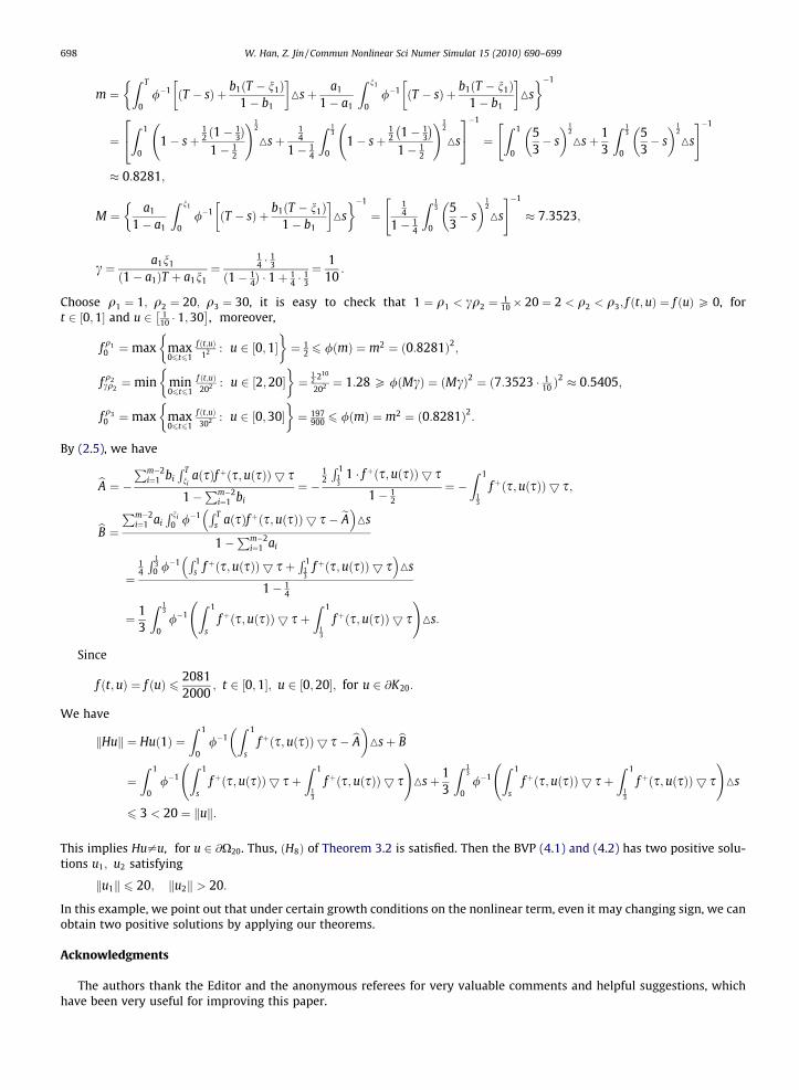
Choose q1 ¼ 1; q2 ¼ 20; q3 ¼ 30, it is easy to check that 1 ¼ q1 < cq2 ¼ 110� 20 ¼ 2 < q2 < q3; f ðt;uÞ ¼ f ðuÞP 0, for
t 2 ½0;1� and u 2 110 � 1;30 �
, moreover,
f q10 ¼max max
06t61
f ðt;uÞ12 : u 2 ½0;1�
� ¼ 1
2 6 /ðmÞ ¼ m2 ¼ ð0:8281Þ2;
f q2cq2¼min min
06t61
f ðt;uÞ202 : u 2 ½2;20�
� ¼
12�2
10
202 ¼ 1:28 P /ðMcÞ ¼ ðMcÞ2 ¼ ð7:3523 � 110 Þ
2 � 0:5405;
f q30 ¼max max
06t61
f ðt;uÞ302 : u 2 ½0;30�
� ¼ 197
900 6 /ðmÞ ¼ m2 ¼ ð0:8281Þ2:
By (2.5), we have
bA ¼ �Pm�2i¼1 bi
R Tni
aðsÞfþðs;uðsÞÞ 5 s
1�Pm�2
i¼1 bi
¼ �12
R 113
1 � fþðs;uðsÞÞ 5 s
1� 12
¼ �Z 1
13
fþðs;uðsÞÞ 5 s;
bB ¼Pm�2i¼1 ai
R ni0 /�1 R T
s aðsÞfþðs;uðsÞÞ 5 s� eA� �Ms
1�Pm�2
i¼1 ai
¼14
R 130 /�1 R 1
s fþðs;uðsÞÞ 5 sþR 1
13
fþðs;uðsÞÞ 5 s� �
Ms
1� 14
¼ 13
Z 13
0/�1
Z 1
sfþðs;uðsÞÞ 5 sþ
Z 1
13
fþðs; uðsÞÞ 5 s !
Ms:
Since
f ðt;uÞ ¼ f ðuÞ 6 20812000
; t 2 ½0;1�; u 2 ½0;20�; for u 2 @K20:
We have
kHuk ¼ Huð1Þ ¼Z 1
0/�1
Z 1
sfþðs; uðsÞÞ 5 s� bA� �
Msþ bB¼Z 1
0/�1
Z 1
sfþðs;uðsÞÞ 5 sþ
Z 1
13
fþðs; uðsÞÞ 5 s !
Msþ 13
Z 13
0/�1
Z 1
sfþðs;uðsÞÞ 5 sþ
Z 1
13
fþðs; uðsÞÞ 5 s !
Ms
6 3 < 20 ¼ kuk:
This implies Hu–u, for u 2 @X20. Thus, ðH8Þ of Theorem 3.2 is satisfied. Then the BVP (4.1) and (4.2) has two positive solu-tions u1; u2 satisfying
ku1k 6 20; ku2k > 20:
In this example, we point out that under certain growth conditions on the nonlinear term, even it may changing sign, we canobtain two positive solutions by applying our theorems.
Acknowledgments
The authors thank the Editor and the anonymous referees for very valuable comments and helpful suggestions, whichhave been very useful for improving this paper.
W. Han, Z. Jin / Commun Nonlinear Sci Numer Simulat 15 (2010) 690–699 699
References
[1] Agarwal RP, O’Regan D. Nonlinear boundary value problems on time scales. Nonlinear Anal 2001;44:527–35.[2] Agarwal RP, Bohner M, Rehak P. Half-linear dynamic equations, Nonlinear analysis and applications: to V. Lakshmikantham on his 80th birthday.
Dordrecht: 2003. p. 1–57.[3] Anderson DR. Solutions to second-order three-point problems on time scales. J Differ Equ Appl 2002;8:673–88.[4] Anderson DR, Avery R, Henderson J. Existence of solutions for a one-dimensional p-Laplacian on time scales. J Differ Equ Appl 2004;10:889–96.[5] Atici FM, Gnseinov GSh. On Green’n functions and positive solutions for boundary value problems on time scales. J Comput Anal Math
2002;141:75–99.[6] Aulbach B, Neidhart L. Integration on measure chain. In: Proc. of the sixth int. conf. on difference equations. BocaRaton, Fl: CRC; 2004. p. 239–52.[7] Bohner M, Peterson A. Dynamic equations on time scales: an introduction with applications. Boston, Cambridge, MA: Birkhäuser; 2001.[8] Bohner M, Peterson A. Advances in dynamic equations on time scales. Cambridge, MA: Birkhäuser Boston; 2003.[9] Dacunha JJ, Davis JM, Singh PK. Existence results for singular three point boundary value problems on time scales. J Math Anal Appl 2004;295:378–91.
[10] Feng HY, Ge W, Jiang M. Multiple positive solutions for m-point boundary-value problems with a one-dimensional p-Laplacian. Nonlinear Anal2008;68:2269–79.
[11] Guo D, Lakshmikanthan V. Nonlinear problems in abstract cones. San Diego: Academic Press; 1988.[12] He ZM. Double positive solutions of three-point boundary value problems for p-Laplacian dynamic equations on time scales. J Comput Appl Math
2005;182:304–15.[13] He ZM. Triple positive solutions of boundary value problems for p-Laplacian dynamic equations on time scales. J Math Anal Appl 2006;321:911–20.[14] Sun JP, Li WT. Existence and nonexistence of positive solutions for second-order time scale systems. Nonlinear Anal 2008;68:3107–14.[15] Lan KQ. Multiple positive solutions of semilinear differential equations with singularities. J Lond Math Soc 2001;63:690–704.[16] Liang SH, Zhang JH. The existence of countably many positive solutions for nonlinear singular m-point boundary-value problems. J Comput Appl Math
2008;214:78–89.[17] Liu BF, Zhang JH. The existence of positive solutions for some nonlinear boundary value problems with linear mixed boundary conditions. J Math Anal
Appl 2005;309:505–16.[18] Luo H, Ma QZ. Positive solutions to a generalized second-order three-point boundary value problem on time scales. Eletron J Differ Equ 2005;17:1–14.[19] Ma D, Du Z, Ge W. Existence and iteration of monotone positive solutions for multipoint boundary value problem with p-Laplacian operator. Comput
Math Appl 2005;50:729–39.[20] Ma RY. Existence of solutions of nonlinear m-point boundary value problem. J Math Anal Appl 2001;256:556–67.[21] Su H, Wang B, Wei Z. Positive solutions of four-point boundary value problems for four-order p-Laplacian dynamic equations on time scales. Eletron J
Differ Equ 2006;78.[22] Su H, Wei Z, Xu F. The existence of countably many positive solutions for a system of nonlinear singular boundary value problems with the p-Laplacian
operator. J Math Anal Appl 2007;325:319–32.[23] Su YH, Li WT, Sun HR. Positive solutions of singular p-Laplacian BVPs with sign changing nonlinearity on time scales. Math Comput Model
2008;48:845–58.[24] Sun HR, Li WT. Multiple Positive solutions for p-Laplacian m-point boundary value problems on time scales. Appl Math Comput 2006;182:478–91.[25] Sun HR, Li WT. Positive solutions for nonlinear three-point boundary value problems on time scales. J Math Anal Appl 2004;299:508–24.[26] Sun HR, Li WT. Positive solutions for nonlinear m-point boundary value problems on time scales. Acta Math Sinica 2006;49:369–80. in Chinese.[27] Wang Y, Ge W. Positive solutions for multipoint boundary value problems with a one-dimensional p-Laplacian. Nonlinear Anal 2007;66:1246–56.