Positive Weights on the Efficient Frontier

Phelim Boyle

Wilfrid Laurier University

August 2012

Acknowledgments

This paper is dedicated to Boyle’s Winter 2012 graduate financeclass at Wilfrid Laurier University as it grew out of one of theirassignments. Thanks to Marco Avellaneda, Jit Seng Chen, WilliamGornall, Anne Mackay, David Melkuev, Christina Park, Dick Roll,Matthew Wang and Terry Zhang for helpful comments.

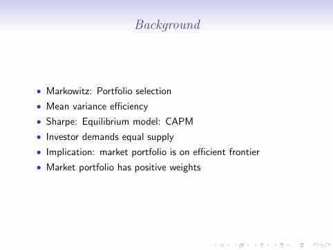
Background

• Markowitz: Portfolio selection

• Mean variance efficiency

• Sharpe: Equilibrium model: CAPM

• Investor demands equal supply

• Implication: market portfolio is on efficient frontier

• Market portfolio has positive weights

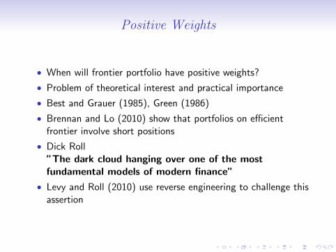
Positive Weights

• When will frontier portfolio have positive weights?

• Problem of theoretical interest and practical importance

• Best and Grauer (1985), Green (1986)

• Brennan and Lo (2010) show that portfolios on efficientfrontier involve short positions

• Dick Roll”The dark cloud hanging over one of the mostfundamental models of modern finance”

• Levy and Roll (2010) use reverse engineering to challenge thisassertion

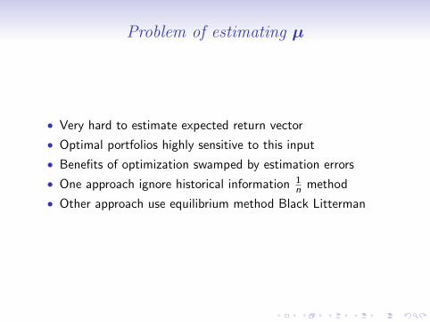
Problem of estimating µ

• Very hard to estimate expected return vector

• Optimal portfolios highly sensitive to this input

• Benefits of optimization swamped by estimation errors

• One approach ignore historical information 1n method

• Other approach use equilibrium method Black Litterman

This paper

• Provides a simple method to obtain a frontier portfolio withpositive weights

• Uses eigenvectors of correlation matrix to construct set oforthogonal portfolios

• If any one of these orthogonal portfolios is on the frontier theothers have the same expected return

• The portfolio corresponding to the largest eigenvalue haspositive weights

• Ensure this portfolio is on the frontier

• This leads to nice results and intuitive interpretations

• Simple and natural way to obtain µ

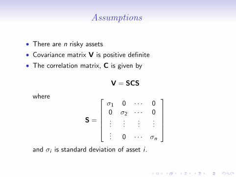
Assumptions

• There are n risky assets

• Covariance matrix V is positive definite

• The correlation matrix, C is given by

V = SCS

where

S =

σ1 0 · · · 00 σ2 · · · 0...

......

...... 0 · · · σn

and σi is standard deviation of asset i .

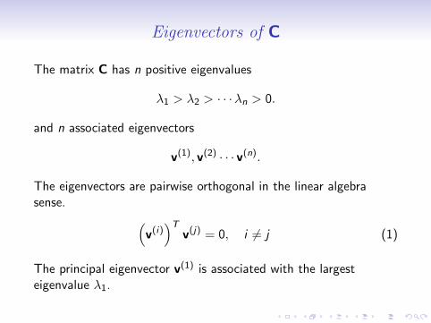
Eigenvectors of C

The matrix C has n positive eigenvalues

λ1 > λ2 > · · ·λn > 0.

and n associated eigenvectors

v(1), v(2) · · · v(n).

The eigenvectors are pairwise orthogonal in the linear algebrasense. (

v(i))T

v(j) = 0, i 6= j (1)

The principal eigenvector v(1) is associated with the largesteigenvalue λ1.

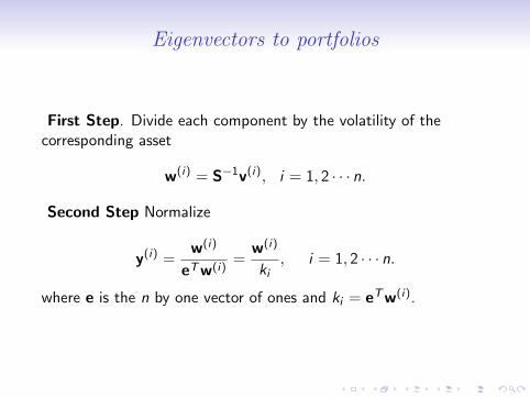
Eigenvectors to portfolios

First Step. Divide each component by the volatility of thecorresponding asset

w(i) = S−1v(i), i = 1, 2 · · · n.

Second Step Normalize

y(i) =w(i)

eTw(i)=

w(i)

ki, i = 1, 2 · · · n.

where e is the n by one vector of ones and ki = eTw(i).

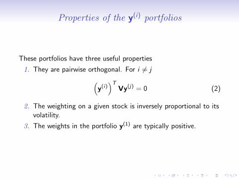
Properties of the y(i) portfolios

These portfolios have three useful properties

1. They are pairwise orthogonal. For i 6= j(y(i))T

Vy(j) = 0 (2)

2. The weighting on a given stock is inversely proportional to itsvolatility.

3. The weights in the portfolio y(1) are typically positive.

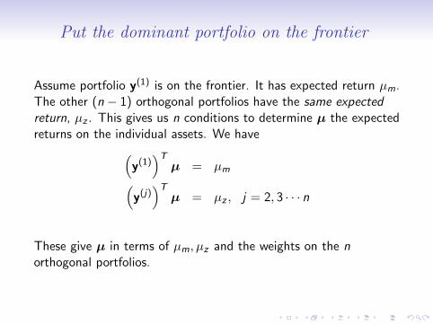
Put the dominant portfolio on the frontier

Assume portfolio y(1) is on the frontier. It has expected return µm.The other (n − 1) orthogonal portfolios have the same expectedreturn, µz . This gives us n conditions to determine µ the expectedreturns on the individual assets. We have(

y(1))T

µ = µm(y(j))T

µ = µz , j = 2, 3 · · · n

These give µ in terms of µm, µz and the weights on the northogonal portfolios.

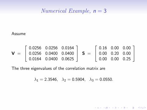
Numerical Example, n = 3

Assume

V =

0.0256 0.0256 0.01640.0256 0.0400 0.04000.0164 0.0400 0.0625

S =

0.16 0.00 0.000.00 0.20 0.000.00 0.00 0.25

The three eigenvalues of the correlation matrix are

λ1 = 2.3546, λ2 = 0.5904, λ3 = 0.0550.

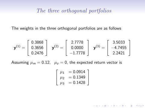
The three orthogonal portfolios

The weights in the three orthogonal portfolios are as follows

y(1) =

0.38680.36560.2476

y(2) =

2.77780.0000−1.7778

y(3) =

3.5033−4.74552.2421

Assuming µm = 0.12, µz = 0, the expected return vector is µ1 = 0.0914

µ2 = 0.1349µ3 = 0.1428

Plot of the three orthogonal portfolios

0 0.05 0.1 0.15 0.2 0.25−0.05

0

0.05

0.1

0.15

0.2

0.25

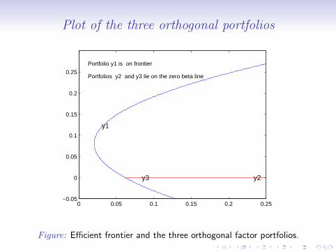
Portfolio y1 is on frontier

Portfolios y2 and y3 lie on the zero beta line

y1

y2y3

Figure: Efficient frontier and the three orthogonal factor portfolios.

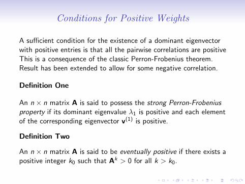
Conditions for Positive Weights

A sufficient condition for the existence of a dominant eigenvectorwith positive entries is that all the pairwise correlations are positiveThis is a consequence of the classic Perron-Frobenius theorem.Result has been extended to allow for some negative correlation.

Definition One

An n × n matrix A is said to possess the strong Perron-Frobeniusproperty if its dominant eigenvalue λ1 is positive and each elementof the corresponding eigenvector v(1) is positive.

Definition Two

An n × n matrix A is said to be eventually positive if there exists apositive integer k0 such that Ak > 0 for all k > k0.

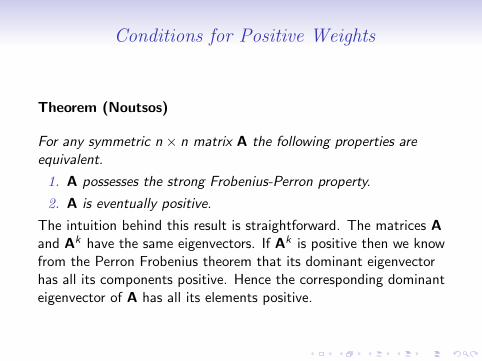
Conditions for Positive Weights

Theorem (Noutsos)

For any symmetric n × n matrix A the following properties areequivalent.

1. A possesses the strong Frobenius-Perron property.

2. A is eventually positive.

The intuition behind this result is straightforward. The matrices Aand Ak have the same eigenvectors. If Ak is positive then we knowfrom the Perron Frobenius theorem that its dominant eigenvectorhas all its components positive. Hence the corresponding dominanteigenvector of A has all its elements positive.

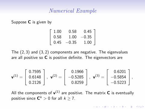
Numerical Example

Suppose C is given by 1.00 0.58 0.450.58 1.00 −0.350.45 −0.35 1.00

The (2, 3) and (3, 2) components are negative. The eigenvaluesare all positive so C is positive definite. The eigenvectors are

v(1) =

0.75950.61480.2126

, v(2) =

0.1966−0.5285

0.8259

, v(3) =

0.6201−0.5854−0.5223

,All the components of v(1) are positive. The matrix C is eventuallypositive since Ck > 0 for all k ≥ 7.

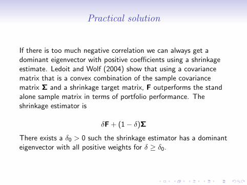
Practical solution

If there is too much negative correlation we can always get adominant eigenvector with positive coefficients using a shrinkageestimate. Ledoit and Wolf (2004) show that using a covariancematrix that is a convex combination of the sample covariancematrix Σ and a shrinkage target matrix, F outperforms the standalone sample matrix in terms of portfolio performance. Theshrinkage estimator is

δF + (1− δ)Σ

There exists a δ0 > 0 such the shrinkage estimator has a dominanteigenvector with all positive weights for δ ≥ δ0.

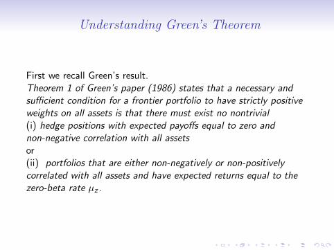
Understanding Green’s Theorem

First we recall Green’s result.Theorem 1 of Green’s paper (1986) states that a necessary andsufficient condition for a frontier portfolio to have strictly positiveweights on all assets is that there must exist no nontrivial(i) hedge positions with expected payoffs equal to zero andnon-negative correlation with all assetsor(ii) portfolios that are either non-negatively or non-positivelycorrelated with all assets and have expected returns equal to thezero-beta rate µz .

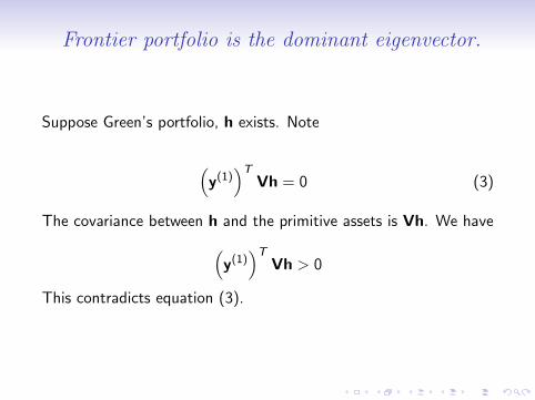
Frontier portfolio is the dominant eigenvector.

Suppose Green’s portfolio, h exists. Note

(y(1))T

Vh = 0 (3)

The covariance between h and the primitive assets is Vh. We have(y(1))T

Vh > 0

This contradicts equation (3).

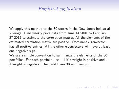
Empirical application

We apply this method to the 30 stocks in the Dow Jones IndustrialAverage. Used weekly price data from June 14 2001 to February27 2012 to estimate the correlation matrix. All the elements of theestimated correlation matrix are positive. Dominant eigenvectorhas all positive entries. All the other eigenvectors will have at leastone negative sign.We use a simple convention to summarize the elements of the 30portfolios. For each portfolio, use +1 if a weight is positive and -1if weight is negative. Then add these 30 numbers up .

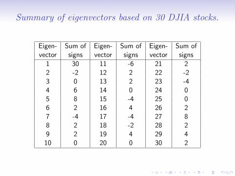
Summary of eigenvectors based on 30 DJIA stocks.

Eigen- Sum of Eigen- Sum of Eigen- Sum ofvector signs vector signs vector signs

1 30 11 -6 21 22 -2 12 2 22 -23 0 13 2 23 -44 6 14 0 24 05 8 15 -4 25 06 2 16 4 26 27 -4 17 -4 27 88 2 18 -2 28 29 2 19 4 29 4

10 0 20 0 30 2

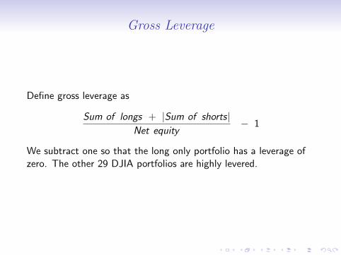
Gross Leverage

Define gross leverage as

Sum of longs + |Sum of shorts|Net equity

− 1

We subtract one so that the long only portfolio has a leverage ofzero. The other 29 DJIA portfolios are highly levered.

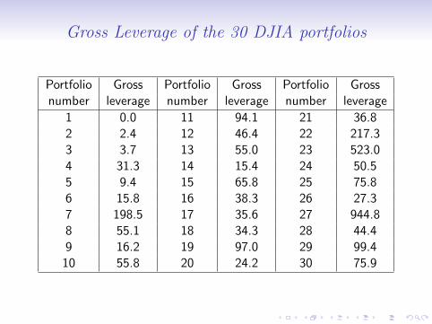
Gross Leverage of the 30 DJIA portfolios

Portfolio Gross Portfolio Gross Portfolio Grossnumber leverage number leverage number leverage

1 0.0 11 94.1 21 36.82 2.4 12 46.4 22 217.33 3.7 13 55.0 23 523.04 31.3 14 15.4 24 50.55 9.4 15 65.8 25 75.86 15.8 16 38.3 26 27.37 198.5 17 35.6 27 944.88 55.1 18 34.3 28 44.49 16.2 19 97.0 29 99.4

10 55.8 20 24.2 30 75.9

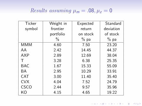
Results assuming µm = .08, µz = 0

Ticker Weight in Expected Standardsymbol frontier return deviation

portfolio on stock of stock% % pa % pa

MMM 4.60 7.50 23.20AA 2.42 14.45 44.37AXP 2.89 12.69 38.04T 3.28 6.38 25.35BAC 1.67 15.33 55.09BA 2.95 10.29 33.91CAT 3.00 11.40 35.40CVX 4.04 7.52 24.79CSCO 2.44 9.57 35.96KO 4.15 4.65 19.22

Robustness of results

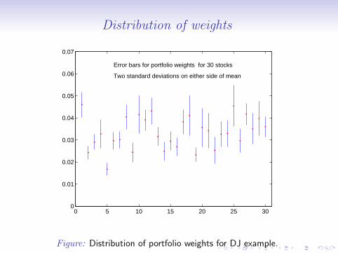
Distribution of weights

0 5 10 15 20 25 300

0.01

0.02

0.03

0.04

0.05

0.06

0.07

Error bars for portfolio weights for 30 stocks

Two standard deviations on either side of mean

Figure: Distribution of portfolio weights for DJ example.

Distribution of expected returns

0 5 10 15 20 25 300

0.02

0.04

0.06

0.08

0.1

0.12

0.14

0.16

0.18

0.2 Error bars for expected return vectors for 30 stocks

Two standard deviations on either side of mean

Figure: Distribution of expected returns for DJ example.

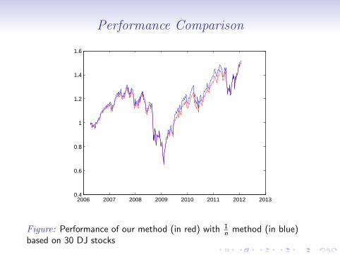
Performance Comparison

2006 2007 2008 2009 2010 2011 2012 20130.4

0.6

0.8

1

1.2

1.4

1.6

Figure: Performance of our method (in red) with 1n method (in blue)

based on 30 DJ stocks

Summary

• Simple approach to find positive portfolio

• Uses just the covariance matrix

• Natural way to obtain the return vector

• Method is robust estimation error

• Performance comparable with 1n results