Positively regular vague matrices

Linear Algebra and its Applications 326 (2001) 85–100www.elsevier.com/locate/laa

Positively regular vague matricesJosef Nedoma

Institute of Mathematics, Academy of Sciences of the Czech Republic, Zitna 25, 115 67 Praha 1,Czech Republic

Received 19 July 1996; accepted 18 September 2000

Submitted by R.A. Brualdi

Abstract

Positive regularity is a common attribute of inaccurate square matrices which can be usedin linear equation systems that provide only nonnegative solutions. It is studied within theframework of vague matrices which can be considered as a generalization of interval matri-ces. Criteria of positive regularity are derived and a method of verifying them is outlined.The exposition concludes with a characterization of the radius of positive regularity. © 2001Elsevier Science Inc. All rights reserved.

Keywords: Vague matrix; Positive regularity; Simultaneous optimization

1. Introduction

The problem of solving systems of linear equations and inequalities with inac-curate data has been drawing attention for more than 30 years. It has been treatedwithin the framework of both the interval analysis and the optimality theory. Dantzig[2] introduced the concept of the generalized linear programming problem (GLPP),the columns of which were convex polyhedral sets. In GLPP, the so-calledoptimisticapproachis used: a solution is considered feasible if it is feasible for at least onerealization of the data. The opposite,pessimistic approachto inaccuracy of the en-tries is used in the semi-infinite programming [3], the inexact programming [14,17]and the inclusive programming [14,15]: a solution is required to satisfy all possiblerealizations of the data. (Cf. [16,17].)

E-mail address:[email protected] (J. Nedoma).

0024-3795/01/$ - see front matter� 2001 Elsevier Science Inc. All rights reserved.PII: S 0 0 2 4 - 3 7 9 5 ( 0 0 ) 0 0 2 7 5 - 5

86 J. Nedoma / Linear Algebra and its Applications 326 (2001) 85–100

The interval analysis uses mostly the optimistic approach. Its significant part dealswith square systems of inaccurate linear equations [1,8,9,11–13]. One of the current-ly discussed topics is the problem of checking regularity of a square interval matrix.Poljak and Rohn [10] proved that this problem is NP-hard.

In this paper, we deal with a more specific concept of regularity that can be con-sidered as a common attribute of inaccurate square matrices which are suitable formodels the solutions of which are supposed to be nonnegative. Such an assumptionis usually accepted in many applications. On the other hand, we study a more generaltype of inaccurate matrices. As it is shown in Section 2, the procedures given belowcan be effectively applied to several interesting types of these matrices. Besides thesimplest case of interval matrices, we discuss the octaedric matrices defined by usingsimple polyhedra of the well-known type and the elliptic matrices, the columns ofwhich can move inn-dimensional ellipsoids. A matrix of the latter type can be usedas a deterministic equivalent of a random matrix with then-dimensional normaldistribution of columns [6].

The following definition was introduced in [5].

Definition 1. Let A1, . . . , An ⊂ Rm be compact convex sets. The set of matrices

AV = {A |A = (

a1, . . . , an), aj ∈ Aj , j = 1, . . . , n

}is called avague matrix.

A vague matrixAV could be equivalently defined as an orderedn-tuple of vaguecolumns, i.e.,AV = (A1, . . . , An).

In this paper, we deal with squaren × n vague matrices only. A square vaguematrix AV is singular if there exists a singularA ∈ AV. Otherwise,AV is regular.The solution set of a vague linear equation systemAVx = b is defined consistentlywith the optimistic approach, i.e.,

X(AV, b

) = {x∣∣ ∃A ∈ AV: Ax = b

}.

Further let

X+(AV, b

) = X(AV, b

) ∩ Rn+ = {x∣∣ x ∈ X

(AV, b

), x � 0

}.

If AV is regular, thenX(AV, b), being a continuous map of a convex compact setAV ⊂ Rn2

, is a connected compact set.

2. Basic properties of positively regular vague matrices

Definition 2. A square vague matrixAV is calledpositively regularif there exists ab ∈ Rn such that

Ax = b has a solution for eachA ∈ AV, (1)

x ∈ X(AV, b

) ⇒ x > 0. (2)

J. Nedoma / Linear Algebra and its Applications 326 (2001) 85–100 87

We can formulate a few plausible assertions which follow immediately from thisdefinition.

Proposition 1. A positively regular vague matrix is regular.

Proof. Consider ab satisfying (1). If the assertion did not hold, then there wouldexist a nontrivial affine subspaceL ∈ X(AV, b), which would contradict condition(2). �

Proposition 2. A ‘one-point’ vague matrixAV = {A} is positively regular if andonly if A is nonsingular.

Proposition 3. LetAV0 be positively regular. Then there exists an open set� ⊃ AV

0in Rn×n such that any vague matrixAV contained in� is positively regular.

Thus, the requirement of positive regularity is not too restricting for a set of smallperturbations of a given nonsingular matrix.

Proposition 4. LetAV be regular and let there exists a b such that(2) holds. ThenAV is positively regular.

Condition (2) can be expressed asX(AV, b) ⊂ int Rn+, where int denotes theinterior of the respective set. The problem of verifying this condition is solved inthe following section. Condition (1) itself, however, can be hardly verified in anoperative way. Therefore, we are going to give a more transparent equivalent of(1), (2).

Consider vector functions

aj (t) : [0,∞) → Rn, j ∈ J = {1, . . . , n}and a variable convex cone

K(t) = {u = λ1a

1(t) + · · · + λnan(t), λj > 0 ∀j ∈ J

}. (3)

Lemma 1. Assume that

(i) aj (t) are continuous in at∗ > 0 and(ii) aj (t∗) /= 0 ∀j ∈ J .

Then ⋂t∈[0,t∗)

K(t) =⋂

t∈[0,t∗]K(t). (4)

Proof. Let us choose ab �∈ K(t∗). According to the well-known separation theorem,there exists a vectorv such thatvTb > 0 andvTu < 0 ∀u ∈ K(t∗). Due to condi-tion (ii), the latter relation is equivalent tovTaj (t∗) < 0 ∀j ∈ J. Thus,vTaj (t) <


0 ∀j ∈ J ∀t ∈ [t∗ − ε, t∗] must hold for a sufficiently smallε > 0, which impliesb �∈ ⋂t∈[0,t∗) K(t). �

Theorem 1. AV is positively regular if and only if the following conditions aresatisfied:

0 �∈ Aj ∀j ∈ J, (5)

∃b: ∅ �= X(AV, b

) ⊂ int Rn+. (6)

Proof. ‘If part’. Choose ab satisfying (6). There exist a nonsingular matrixA0 = (0a1, . . . , 0an) ∈ AV and anx ∈ Rn such thatA0x = b. Choose another matrixA = (a1, . . . , an) ∈ AV arbitrarily and denoteA(t) = (a1(t), . . . , an(t)) = (1 − t)

A0 + tA. Further, let

t∗ = sup{t |A(τ) is nonsingular forτ ∈ [0, t)}. (7)

Let us suppose thatt∗ < 1. Thenb ∈ K(t) for 0 � t < t∗ due to (6). According toLemma 1, we haveb ∈ K(t∗), which means thatA(t∗)x = b has a solution. Con-sequently,A(t∗) is nonsingular due to (6) again. Relation (7), however, implies thatA(t∗) is singular because the set of all nonsingular matrices is open. This contradic-tion yieldst∗ > 1, which means thatA is nonsingular and, consequently,AV is reg-ular. Then the positive regularity ofAV follows from Proposition 4.

‘Only if’ part follows immediately from Definition 1. �

The natural assumption (5) that none of the matrices ofAV contains a zero col-umn can be easily verified. If there exists a right-hand side vector that produce onlypositive solutions, we have an interesting equivalence:

Theorem 2. If condition(6) holds, then the following properties are equivalent:

(i) 0 �∈ Aj ∀j ∈ J ;(ii) AV is positively regular;(iii) AV is regular.

Proof. (i) ⇒ (ii) follows from Theorem 1, (ii)⇒ (iii) holds due to Proposition 1.The rest is plausible. �

Corollary 1. Assume that(6) holds and letX(AV, b) be bounded. ThenAV is pos-itively regular.

Let us define

Y(AV) = {

y∣∣X(AV, y

) ⊂ Rn+}. (8)

ProvidedX(AV, b) ⊂ int Rn+ holds for ab ∈ Rn, the same relation is kept forsufficiently small perturbations ofb. Hence, condition (6) is equivalent to


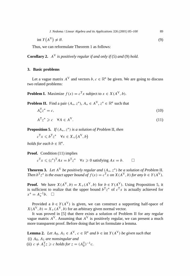
int Y(AV) �= ∅. (9)

Thus, we can reformulate Theorem 1 as follows:

Corollary 2. AV is positively regular if and only if(5) and(9) hold.

3. Basic problems

Let a vague matrixAV and vectorsb, c ∈ Rn be given. We are going to discusstwo related problems:

Problem I. Maximizef (x) = cTx subject tox ∈ X(AV, b).

Problem II. Find a pair(A∗, z∗), A∗ ∈ AV, z∗ ∈ Rn such that

AT∗z∗ = c, (10)

ATz∗ � c ∀A ∈ AV . (11)

Proposition 5. If (A∗, z∗) is a solution of ProblemII, then

cTx � bTz∗ ∀x ∈ X+(AV, b

)holds for eachb ∈ Rn.

Proof. Condition (11) implies

cTx � (z∗)TAx = bTz∗ ∀x � 0 satisfyingAx = b. �

Theorem 3. LetAV be positively regular and(A∗, z∗) be a solution of ProblemII .ThenbTz∗ is the exact upper bound off (x) = cTx onX(AV, b) for anyb ∈ Y (AV).

Proof. We haveX(AV, b) = X+(AV, b) for b ∈ Y (AV). Using Proposition 5, itis sufficient to realize that the upper boundbTz∗ of cTx is actually achieved forx∗ = A−1∗ b. �

Provided ab ∈ Y (AV) is given, we can construct a supporting half-space ofX(AV, b) = X+(AV, b) for an arbitrary given normal vector.

It was proved in [5] that there exists a solution of Problem II for any regularvague matrixAV. Assuming thatAV is positively regular, we can present a muchmore transparent proof. Before doing that let us formulate a lemma.

Lemma 2. LetA0, A1 ∈ AV, c ∈ Rn andb ∈ int Y (AV) be given such that

(i) A0, A1 are nonsingular and(ii) c /= AT

1z � c holds forz = (AT0)

−1c.


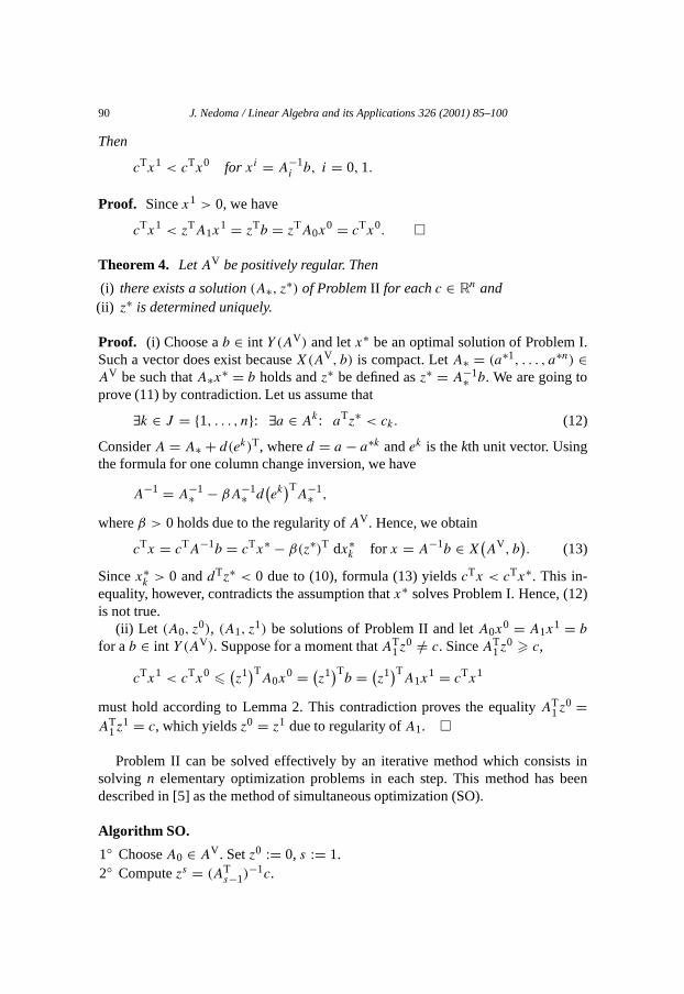
Then

cTx1 < cTx0 for xi = A−1i b, i = 0,1.

Proof. Sincex1 > 0, we have

cTx1 < zTA1x1 = zTb = zTA0x

0 = cTx0. �

Theorem 4. LetAV be positively regular. Then

(i) there exists a solution(A∗, z∗) of ProblemII for eachc ∈ Rn and(ii) z∗ is determined uniquely.

Proof. (i) Choose ab ∈ int Y (AV) and letx∗ be an optimal solution of Problem I.Such a vector does exist becauseX(AV, b) is compact. LetA∗ = (a∗1, . . . , a∗n) ∈AV be such thatA∗x∗ = b holds andz∗ be defined asz∗ = A−1∗ b. We are going toprove (11) by contradiction. Let us assume that

∃k ∈ J = {1, . . . , n}: ∃a ∈ Ak: aTz∗ < ck. (12)

ConsiderA = A∗ + d(ek)T, whered = a − a∗k andek is thekth unit vector. Usingthe formula for one column change inversion, we have

A−1 = A−1∗ − βA−1∗ d(ek)T

A−1∗ ,

whereβ > 0 holds due to the regularity ofAV. Hence, we obtain

cTx = cTA−1b = cTx∗ − β(z∗)T dx∗k for x = A−1b ∈ X

(AV, b

). (13)

Sincex∗k > 0 anddTz∗ < 0 due to (10), formula (13) yieldscTx < cTx∗. This in-

equality, however, contradicts the assumption thatx∗ solves Problem I. Hence, (12)is not true.

(ii) Let (A0, z0), (A1, z

1) be solutions of Problem II and letA0x0 = A1x

1 = b

for ab ∈ int Y (AV). Suppose for a moment thatAT1z

0 /= c. SinceAT1z

0 � c,

cTx1 < cTx0 �(z1)TA0x

0 = (z1)Tb = (

z1)TA1x1 = cTx1

must hold according to Lemma 2. This contradiction proves the equalityAT1z

0 =AT

1z1 = c, which yieldsz0 = z1 due to regularity ofA1. �

Problem II can be solved effectively by an iterative method which consists insolving n elementary optimization problems in each step. This method has beendescribed in [5] as the method of simultaneous optimization (SO).

Algorithm SO.

1◦ ChooseA0 ∈ AV. Setz0 := 0, s := 1.2◦ Computezs = (AT

s−1)−1c.


3◦ FindAs = (sa1, . . . , san) ∈ AV such that(zs)Tsaj = min

{(zs)T

ξ∣∣ ξ ∈ Aj

}, j ∈ J. (14)

4◦ If zs /= zs−1, then sets := s + 1 and go to 2◦.5◦ If zs = zs−1, then END.

A simplified convergence proof of this algorithm in comparison with that givenin [5] is demonstrated below. (Cf. also [7].)

Theorem 5. LetAV be positively regular. Then the following assertions hold:

(i) The sequence{zs} produced by Algorithm SO converges for anyA0 ∈ AV.(ii) If z∗ = limk→∞ zs andA∗ is an accumulation point of{As}, then(A∗, z∗) is a

solution of ProblemII .

Proof. (i) The sequence{zs} is bounded due to the regularity ofAV. We wantto show that it has a unique accumulation point: choose ab ∈ int Y (AV) and de-notexs = A−1

s b � 0. Due to 2◦ and 3◦ we have(zs+1)Tb = (zs+1)TAsxs = cTxs �

(zs)TAsxs = (zs)Tb or(

zs+1 − zs)T

b � 0, s = 0,1, . . . (15)

For an arbitrary pairz∗, z∗∗ of accumulation points of{zs}, relation (15) implies(z∗∗ − z∗) = 0 ∀b ∈ int Y

(AV).

This condition, however, can be fulfilled only ifz∗∗ = z∗. Consequently,zs → z∗.(ii) The assertion follows from (14). �

Apparently, the vectorb ∈ Y (AV) mentioned in the proof is not used in the algo-rithm. If Algorithm SO fails, it means that such a vector does not exist and, conse-quently,AV is not positively regular. Positive regularity, however, is not a necessarycondition of convergence. In the case of positively regular polyhedral vague matrixAV, the solution of (14) can be found among the vertices ofAj . Then, Algorithm SOis finite since there is a finite number of vertices.

The form of elementary optimization problems

min{zTξ

∣∣ ξ ∈ Aj}, (16)

which are to be solved in step 3◦, depends on the way in which the vague matrixAV

is defined. Let us consider a few alternatives:

Interval matrix:

AV = {A∣∣D � A � D

}, D = (

di,j

), D = (

di,j

). (17)

Then (16) takes on the form

minimize zTξ subject to dij � ξi � dij , i ∈ J. (18)


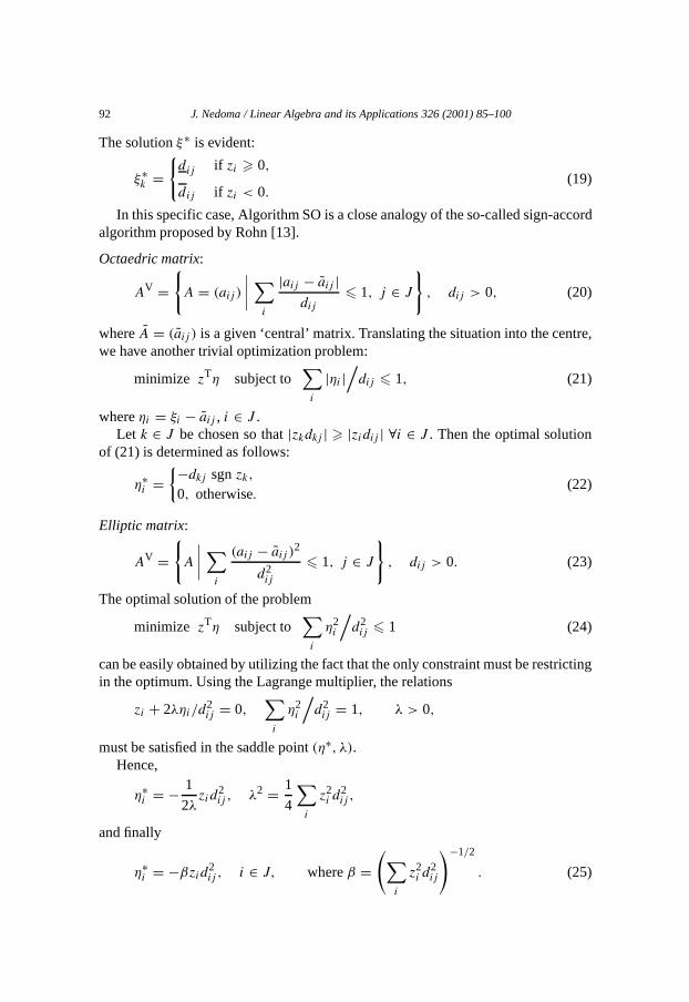
The solutionξ∗ is evident:

ξ∗k =

{dij if zi � 0,

dij if zi < 0.(19)

In this specific case, Algorithm SO is a close analogy of the so-called sign-accordalgorithm proposed by Rohn [13].

Octaedric matrix:

AV ={A = (aij )

∣∣∣∣ ∑i

|aij − aij |dij

� 1, j ∈ J

}, dij > 0, (20)

whereA = (aij ) is a given ‘central’ matrix. Translating the situation into the centre,we have another trivial optimization problem:

minimize zTη subject to∑i

|ηi |/dij � 1, (21)

whereηi = ξi − aij , i ∈ J .Let k ∈ J be chosen so that|zkdkj | � |zidij | ∀i ∈ J . Then the optimal solution

of (21) is determined as follows:

η∗i =

{−dkj sgnzk,0, otherwise.

(22)

Elliptic matrix:

AV ={A

∣∣∣∣ ∑i

(aij − aij )2

d2ij

� 1, j ∈ J

}, dij > 0. (23)

The optimal solution of the problem

minimize zTη subject to∑i

η2i

/d2ij � 1 (24)

can be easily obtained by utilizing the fact that the only constraint must be restrictingin the optimum. Using the Lagrange multiplier, the relations

zi + 2ληi/d2ij = 0,

∑i

η2i

/d2ij = 1, λ > 0,

must be satisfied in the saddle point(η∗, λ).Hence,

η∗i = − 1

2λzid

2ij , λ2 = 1

4

∑i

z2i d

2ij ,

and finally

η∗i = −βzid

2ij , i ∈ J, whereβ =

(∑i

z2i d

2ij

)−1/2

. (25)


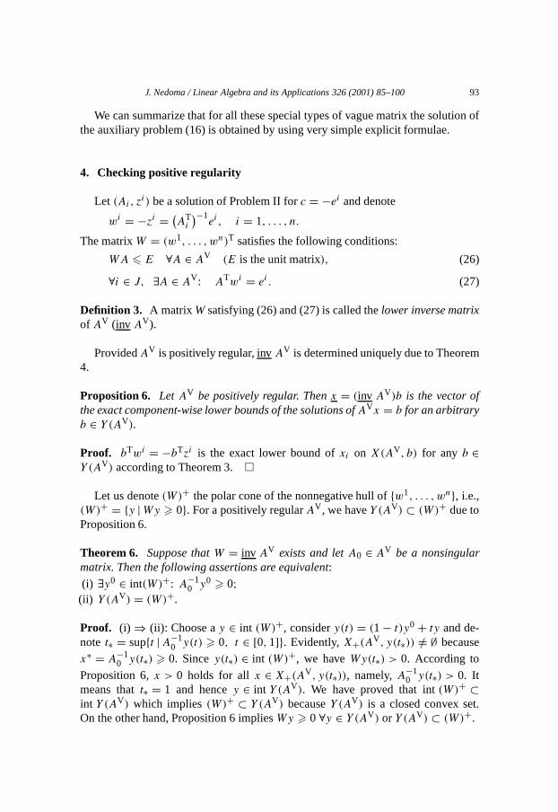
We can summarize that for all these special types of vague matrix the solution ofthe auxiliary problem (16) is obtained by using very simple explicit formulae.

4. Checking positive regularity

Let (Ai, zi) be a solution of Problem II forc = −ei and denote

wi = −zi = (AT

i

)−1ei, i = 1, . . . , n.

The matrixW = (w1, . . . , wn)T satisfies the following conditions:

WA � E ∀A ∈ AV (E is the unit matrix), (26)

∀i ∈ J, ∃A ∈ AV: ATwi = ei. (27)

Definition 3. A matrix Wsatisfying (26) and (27) is called thelower inverse matrixof AV (inv AV).

ProvidedAV is positively regular, invAV is determined uniquely due to Theorem4.

Proposition 6. Let AV be positively regular. Thenx = (inv AV)b is the vector ofthe exact component-wise lower bounds of the solutions ofAVx = b for an arbitraryb ∈ Y (AV).

Proof. bTwi = −bTzi is the exact lower bound ofxi on X(AV, b) for any b ∈Y (AV) according to Theorem 3.�

Let us denote(W)+ the polar cone of the nonnegative hull of{w1, . . . , wn}, i.e.,(W)+ = {y |Wy � 0}. For a positively regularAV, we haveY (AV) ⊂ (W)+ due toProposition 6.

Theorem 6. Suppose thatW = inv AV exists and letA0 ∈ AV be a nonsingularmatrix. Then the following assertions are equivalent:

(i) ∃y0 ∈ int(W)+: A−10 y0 � 0;

(ii) Y (AV) = (W)+.

Proof. (i) ⇒ (ii): Choose ay ∈ int (W)+, considery(t) = (1 − t)y0 + ty and de-note t∗ = sup{t |A−1

0 y(t) � 0, t ∈ [0,1]}. Evidently,X+(AV, y(t∗)) /= ∅ becausex∗ = A−1

0 y(t∗) � 0. Sincey(t∗) ∈ int (W)+, we haveWy(t∗) > 0. According to

Proposition 6,x > 0 holds for all x ∈ X+(AV, y(t∗)), namely,A−10 y(t∗) > 0. It

means thatt∗ = 1 and hencey ∈ int Y (AV). We have proved that int(W)+ ⊂int Y (AV) which implies(W)+ ⊂ Y (AV) becauseY (AV) is a closed convex set.On the other hand, Proposition 6 impliesWy � 0 ∀y ∈ Y (AV) or Y (AV) ⊂ (W)+.


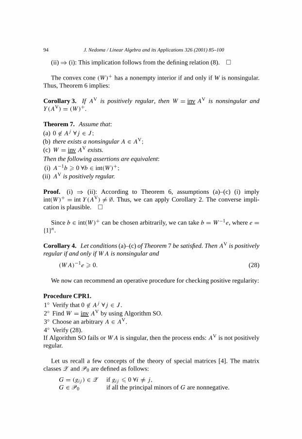
(ii) ⇒ (i): This implication follows from the defining relation (8).�

The convex cone(W)+ has a nonempty interior if and only ifW is nonsingular.Thus, Theorem 6 implies:

Corollary 3. If AV is positively regular, then W = inv AV is nonsingular andY (AV) = (W)+.

Theorem 7. Assume that:

(a) 0 �∈ Aj ∀j ∈ J ;(b) there exists a nonsingularA ∈ AV;(c) W = inv AV exists.

Then the following assertions are equivalent:

(i) A−1b � 0 ∀b ∈ int(W)+;(ii) AV is positively regular.

Proof. (i) ⇒ (ii): According to Theorem 6, assumptions (a)–(c) (i) implyint(W)+ = int Y (AV) �= ∅. Thus, we can apply Corollary 2. The converse impli-cation is plausible. �

Sinceb ∈ int(W)+ can be chosen arbitrarily, we can takeb = W−1e, wheree ={1}n.

Corollary 4. Let conditions(a)–(c) of Theorem7 be satisfied. ThenAV is positivelyregular if and only ifWA is nonsingular and

(WA)−1e � 0. (28)

We now can recommend an operative procedure for checking positive regularity:

Procedure CPR1.1◦ Verify that 0 �∈ Aj ∀j ∈ J .2◦ FindW = inv AV by using Algorithm SO.3◦ Choose an arbitraryA ∈ AV.4◦ Verify (28).If Algorithm SO fails orWA is singular, then the process ends:AV is not positivelyregular.

Let us recall a few concepts of the theory of special matrices [4]. The matrixclassesZ andP0 are defined as follows:

G = (gij ) ∈ Z if gij � 0 ∀i /= j,

G ∈ P0 if all the principal minors ofG are nonnegative.


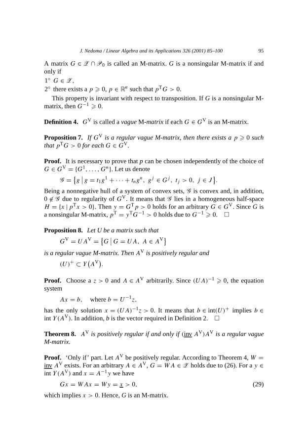
A matrix G ∈ Z ∩ P0 is called an M-matrix.G is a nonsingular M-matrix if andonly if

1◦ G ∈ Z,

2◦ there exists ap � 0,p ∈ Rn such thatpTG > 0.

This property is invariant with respect to transposition. IfG is a nonsingular M-matrix, thenG−1 � 0.

Definition 4. GV is called avagueM-matrix if eachG ∈ GV is an M-matrix.

Proposition 7. If GV is a regular vague M-matrix, then there exists ap � 0 suchthatpTG > 0 for eachG ∈ GV .

Proof. It is necessary to prove thatp can be chosen independently of the choice ofG ∈ GV = {G1, . . . ,Gn}. Let us denote

G = {g∣∣ g = t1g

1 + · · · + tngn, gj ∈ Gj, tj > 0, j ∈ J

}.

Being a nonnegative hull of a system of convex sets,G is convex and, in addition,0 �∈ G due to regularity ofGV. It means thatG lies in a homogeneous half-spaceH = {x |pTx > 0}. Theny = GTp > 0 holds for an arbitraryG ∈ GV. SinceG isa nonsingular M-matrix,pT = yTG−1 > 0 holds due toG−1 � 0. �

Proposition 8. Let U be a matrix such that

GV = UAV = {G∣∣G = UA, A ∈ AV}

is a regular vague M-matrix. ThenAV is positively regular and

(U)+ ⊂ Y(AV).

Proof. Choose az > 0 andA ∈ AV arbitrarily. Since(UA)−1 � 0, the equationsystem

Ax = b, whereb = U−1z,

has the only solutionx = (UA)−1z > 0. It means thatb ∈ int(U)+ implies b ∈int Y (AV). In addition,b is the vector required in Definition 2.�

Theorem 8. AV is positively regular if and only if(inv AV)AV is a regular vagueM-matrix.

Proof. ‘Only if’ part. Let AV be positively regular. According to Theorem 4,W =inv AV exists. For an arbitraryA ∈ AV, G = WA ∈ Z holds due to (26). For ay ∈int Y (AV) andx = A−1y we have

Gx = WAx = Wy = x > 0, (29)

which impliesx > 0. Hence,G is an M-matrix.


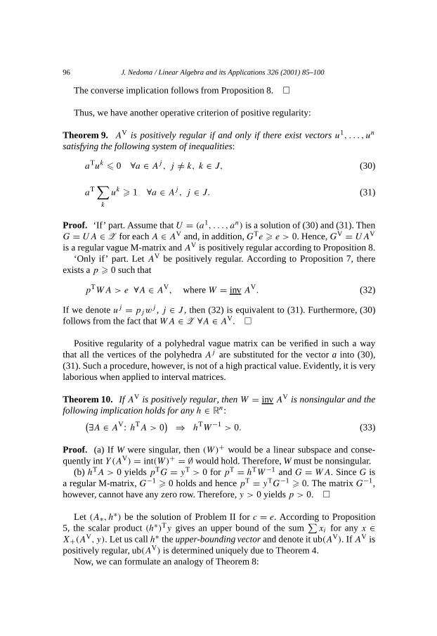
The converse implication follows from Proposition 8.�

Thus, we have another operative criterion of positive regularity:

Theorem 9. AV is positively regular if and only if there exist vectorsu1, . . . , un

satisfying the following system of inequalities:

aTuk � 0 ∀a ∈ Aj , j /= k, k ∈ J, (30)

aT∑k

uk � 1 ∀a ∈ Aj , j ∈ J. (31)

Proof. ‘If’ part. Assume thatU = (a1, . . . , an) is a solution of (30) and (31). ThenG = UA ∈ Z for eachA ∈ AV and, in addition,GTe � e > 0. Hence,GV = UAV

is a regular vague M-matrix andAV is positively regular according to Proposition 8.‘Only if’ part. Let AV be positively regular. According to Proposition 7, there

exists ap � 0 such that

pTWA > e ∀A ∈ AV, whereW = inv AV . (32)

If we denoteuj = pjwj , j ∈ J , then (32) is equivalent to (31). Furthermore, (30)

follows from the fact thatWA ∈ Z ∀A ∈ AV. �

Positive regularity of a polyhedral vague matrix can be verified in such a waythat all the vertices of the polyhedraAj are substituted for the vectora into (30),(31). Such a procedure, however, is not of a high practical value. Evidently, it is verylaborious when applied to interval matrices.

Theorem 10. If AV is positively regular, thenW = inv AV is nonsingular and thefollowing implication holds for anyh ∈ Rn:(∃A ∈ AV: hTA > 0

) ⇒ hTW−1 > 0. (33)

Proof. (a) If W were singular, then(W)+ would be a linear subspace and conse-quently intY (AV) = int(W)+ = ∅ would hold. Therefore,W must be nonsingular.

(b) hTA > 0 yieldspTG = yT > 0 for pT = hTW−1 andG = WA. SinceG isa regular M-matrix,G−1 � 0 holds and hencepT = yTG−1 � 0. The matrixG−1,however, cannot have any zero row. Therefore,y > 0 yieldsp > 0. �

Let (A∗, h∗) be the solution of Problem II forc = e. According to Proposition5, the scalar product(h∗)Ty gives an upper bound of the sum

∑xi for any x ∈

X+(AV, y). Let us callh∗ theupper-bounding vectorand denote it ub(AV). If AV ispositively regular, ub(AV) is determined uniquely due to Theorem 4.

Now, we can formulate an analogy of Theorem 8:


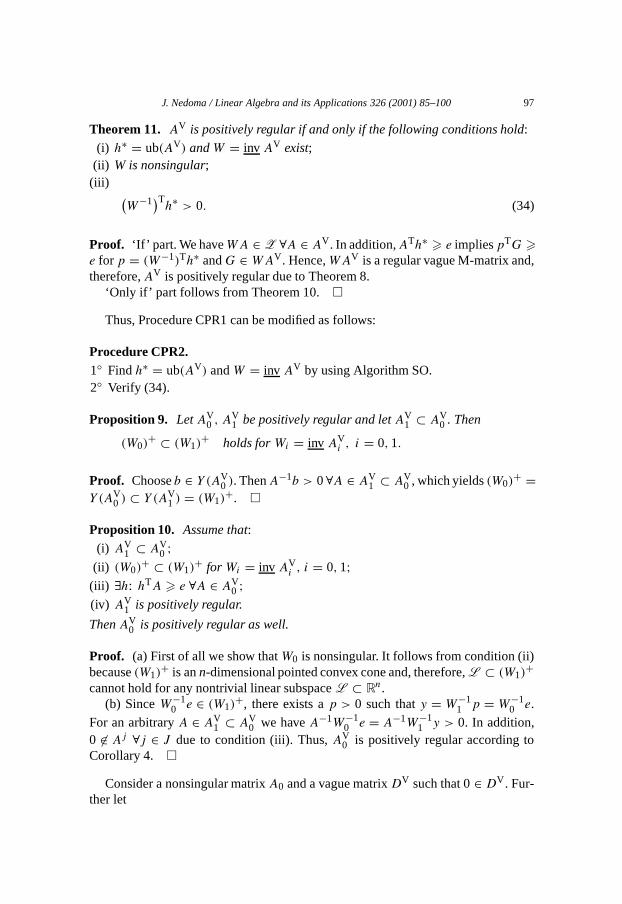
Theorem 11. AV is positively regular if and only if the following conditions hold:

(i) h∗ = ub(AV) andW = inv AV exist;(ii) W is nonsingular;(iii) (

W−1)Th∗ > 0. (34)

Proof. ‘If’ part. We haveWA ∈ Z ∀A ∈ AV. In addition,ATh∗ � e impliespTG �e for p = (W−1)Th∗ andG ∈ WAV. Hence,WAV is a regular vague M-matrix and,therefore,AV is positively regular due to Theorem 8.

‘Only if’ part follows from Theorem 10. �

Thus, Procedure CPR1 can be modified as follows:

Procedure CPR2.1◦ Findh∗ = ub(AV) andW = inv AV by using Algorithm SO.2◦ Verify (34).

Proposition 9. LetAV0 , A

V1 be positively regular and letAV

1 ⊂ AV0 . Then

(W0)+ ⊂ (W1)

+ holds forWi = inv AVi , i = 0,1.

Proof. Chooseb ∈ Y (AV0 ). ThenA−1b > 0∀A ∈ AV

1 ⊂ AV0 , which yields(W0)

+ =Y (AV

0 ) ⊂ Y (AV1 ) = (W1)

+. �

Proposition 10. Assume that:

(i) AV1 ⊂ AV

0 ;(ii) (W0)

+ ⊂ (W1)+ for Wi = inv AV

i , i = 0,1;(iii) ∃h: hTA � e ∀A ∈ AV

0 ;(iv) AV

1 is positively regular.

ThenAV0 is positively regular as well.

Proof. (a) First of all we show thatW0 is nonsingular. It follows from condition (ii)because(W1)

+ is ann-dimensional pointed convex cone and, therefore,L ⊂ (W1)+

cannot hold for any nontrivial linear subspaceL ⊂ Rn.(b) SinceW−1

0 e ∈ (W1)+, there exists ap > 0 such thaty = W−1

1 p = W−10 e.

For an arbitraryA ∈ AV1 ⊂ AV

0 we haveA−1W−10 e = A−1W−1

1 y > 0. In addition,0 �∈ Aj ∀j ∈ J due to condition (iii). Thus,AV

0 is positively regular according toCorollary 4. �

Consider a nonsingular matrixA0 and a vague matrixDV such that 0∈ DV. Fur-ther let


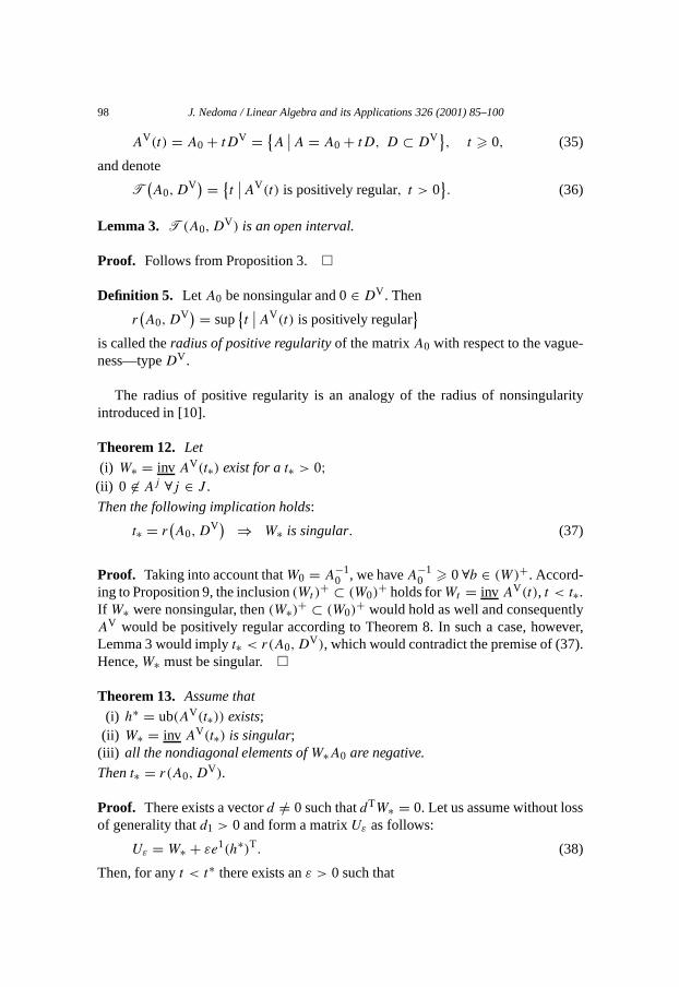
AV(t) = A0 + tDV = {A∣∣A = A0 + tD, D ⊂ DV}, t � 0, (35)

and denote

T(A0,D

V) = {t∣∣AV(t) is positively regular, t > 0

}. (36)

Lemma 3. T(A0,DV) is an open interval.

Proof. Follows from Proposition 3. �

Definition 5. Let A0 be nonsingular and 0∈ DV. Then

r(A0,D

V) = sup{t∣∣AV(t) is positively regular

}is called theradius of positive regularityof the matrixA0 with respect to the vague-ness—typeDV.

The radius of positive regularity is an analogy of the radius of nonsingularityintroduced in [10].

Theorem 12. Let

(i) W∗ = inv AV(t∗) exist for at∗ > 0;(ii) 0 �∈ Aj ∀j ∈ J .

Then the following implication holds:

t∗ = r(A0,D

V) ⇒ W∗ is singular. (37)

Proof. Taking into account thatW0 = A−10 , we haveA−1

0 � 0 ∀b ∈ (W)+. Accord-ing to Proposition 9, the inclusion(Wt )

+ ⊂ (W0)+ holds forWt = inv AV(t), t < t∗.

If W∗ were nonsingular, then(W∗)+ ⊂ (W0)+ would hold as well and consequently

AV would be positively regular according to Theorem 8. In such a case, however,Lemma 3 would implyt∗ < r(A0,D

V), which would contradict the premise of (37).Hence,W∗ must be singular. �

Theorem 13. Assume that

(i) h∗ = ub(AV(t∗)) exists;(ii) W∗ = inv AV(t∗) is singular;(iii) all the nondiagonal elements ofW∗A0 are negative.

Thent∗ = r(A0,DV).

Proof. There exists a vectord /= 0 such thatdTW∗ = 0. Let us assume without lossof generality thatd1 > 0 and form a matrixUε as follows:

Uε = W∗ + εe1(h∗)T. (38)

Then, for anyt < t∗ there exists anε > 0 such that


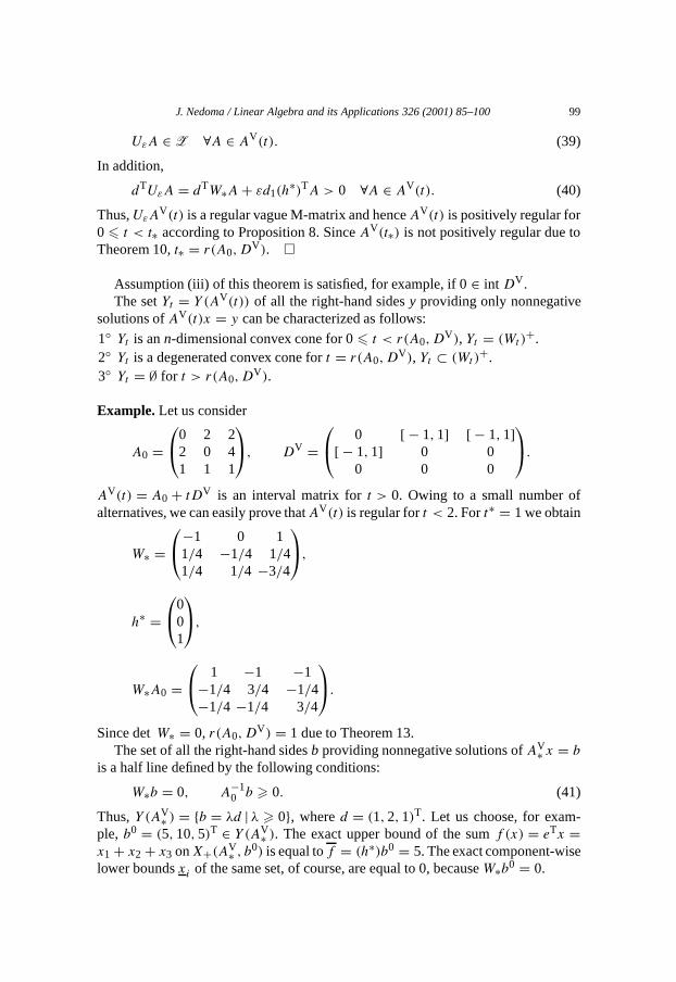
UεA ∈ Z ∀A ∈ AV(t). (39)

In addition,

dTUεA = dTW∗A + εd1(h∗)TA > 0 ∀A ∈ AV(t). (40)

Thus,UεAV(t) is a regular vague M-matrix and henceAV(t) is positively regular for

0 � t < t∗ according to Proposition 8. SinceAV(t∗) is not positively regular due toTheorem 10,t∗ = r(A0,D

V). �

Assumption (iii) of this theorem is satisfied, for example, if 0∈ int DV.The setYt = Y (AV(t)) of all the right-hand sidesy providing only nonnegative

solutions ofAV(t)x = y can be characterized as follows:

1◦ Yt is ann-dimensional convex cone for 0� t < r(A0,DV), Yt = (Wt )

+.2◦ Yt is a degenerated convex cone fort = r(A0,D

V), Yt ⊂ (Wt )+.

3◦ Yt = ∅ for t > r(A0,DV).

Example. Let us consider

A0 =0 2 2

2 0 41 1 1

, DV =

0 [ − 1,1] [ − 1,1]

[ − 1,1] 0 00 0 0

.

AV(t) = A0 + tDV is an interval matrix fort > 0. Owing to a small number ofalternatives, we can easily prove thatAV(t) is regular fort < 2. Fort∗ = 1 we obtain

W∗ =−1 0 1

1/4 −1/4 1/41/4 1/4 −3/4

,

h∗ =0

01

,

W∗A0 = 1 −1 −1

−1/4 3/4 −1/4−1/4 −1/4 3/4

.

Since detW∗ = 0, r(A0,DV) = 1 due to Theorem 13.

The set of all the right-hand sidesb providing nonnegative solutions ofAV∗ x = b

is a half line defined by the following conditions:

W∗b = 0, A−10 b � 0. (41)

Thus,Y (AV∗ ) = {b = λd | λ � 0}, whered = (1,2,1)T. Let us choose, for exam-ple, b0 = (5,10,5)T ∈ Y (AV∗ ). The exact upper bound of the sumf (x) = eTx =x1 + x2 + x3 onX+(AV∗ , b0) is equal tof = (h∗)b0 = 5. The exact component-wiselower boundsxi of the same set, of course, are equal to 0, becauseW∗b0 = 0.


In order to find the lower boundf = min{f (x) | x ∈ X+(AV∗ , b0)}, let us compute

g∗ = −ub(−AV∗ ) = (0,0,1)T. Hence,f = (g∗)Tb0 = 5. We can conclude that foranyt ∈ [0,1), AV(t) is positively regular and

X(AV(t), b0) ⊂ X

(AV∗ , b0) ⊂ {

x∣∣ eTx = 5, x � 0

}. (42)

Acknowledgement

This work was supported by the Czech Republic Grant Agency under the grantNo. GACR 201/95/1484.

References

[1] W. Barth, E. Nuding, Optimale lösung von intervallgleichungssystemen, Computing 12 (1974) 117–125.

[2] G.B. Dantzig, Linear Programming and Extensions, Princeton University Press, Princeton, NJ, 1973.[3] A.V. Fiacco, K.O. Kortanek (Eds.), Semi-infinite Programming and Applications, An International

Symposium, Austin, Texas, 1981, Lecture Notes in Economics and Mathematical Systems, Springer,Berlin, 1981.

[4] M. Fiedler, Special Matrices and Their Application in Numerical Mathematics, Martinus NijhossPubl. & SNTL, Dordrecht, 1986.

[5] J. Nedoma, Vague matrices in linear programming, Ann. Oper. Res. 47 (1993) 483–496.[6] J. Nedoma, Sign-stable solutions of column-vague linear equation systems, Reliable Computing 3

(1997) 173–180.[7] J. Nedoma, Inaccurate linear equation system with a restricted-rank error matrix, Linear and Multi-

linear Algebra 44 (1998) 29–44.[8] W. Oettli, On the solution set of a linear system with inaccurate coefficients, SIAM J. Numer. Anal.

2 (1965) 115–118.[9] W. Oettli, W. Prager, Compatibility of approximate solution of linear equations with given error

bounds for coefficients and right-hand sides, Numer. Math. 6 (1964) 405–409.[10] S. Poljak, J. Rohn, Checking robust nonsingularity is NP-hard, Math. Control Signals Systems 6

(1993) 1–9.[11] J. Rohn, Systems of linear interval equations, Linear Algebra Appl. 126 (1989) 39–78.[12] J. Rohn, On noncovexity of the solution set of a system of linear interval equations, BIT 30 (1989)

161–165.[13] J. Rohn, V. Kreinovich, Computing exact componentwise bounds on solution of linear systems with

interval data is NP-hard, SIAM J. Matrix Anal. Appl. 16 (1995) 415–420.[14] A.L. Soyster, Convex programming with set-inclusive constraints and applications to inexact linear

programming, Oper. Res. 21 (1973) 1154–1157.[15] A.L. Soyster, A duality theory for convex programming with set-inclusive constraints, Oper. Res. 22

(1974) 892–898.[16] J. Tichtschke, R. Hettich, G. Still, Connetions between generalized, inexact and semi-infinite linear

programming, ZOR-Methods Models Oper. Res. 33 (1989) 67–382.[17] D.J. Thuente, Duality theory for generalized linear programs with computational methods, Oper.

Res. 28 (1980) 1005–1011.

Documents

Positively regular vague matrices