POST-FIRE ASSOCIATIONS OF BUTTERFLY BEHAVIOR,

OCCUPANCY, AND ABUNDANCE WITH

ENVIRONMENTAL VARIABLES AND NECTAR SOURCES

IN THE SIERRA NEVADA, CALIFORNIA

A DISSERTATION SUBMITTED TO THE FACULTY OF

THE UNIVERSITY OF MINNESOTA

BY

DAVID THOMAS PAVLIK

IN PARTIAL FULFILLMENT OF THE REQUIREMENTS FOR

THE DEGREE OF MASTER OF SCIENCE

ADVISER: ROBERT B. BLAIR

DECEMBER 2015

© David Thomas Pavlik 2015

i

Acknowledgments

I am most grateful to my committee for their dedication and passion for this project and

for pushing me outside of my comfort zone, both logistically and statistically. Rob, thank

you for accepting me into your lab and for keeping me grounded. You always nudged me

in the right direction with a light-hearted attitude. Erica, thanks for “suggesting” to Rob

to answer my first email, and for guiding me through all aspects of this research. Karen,

thanks for brainstorming with me about the direction of this project, especially in the

beginning, and for your butterfly expertise and research ideas.

This project would not have been possible without my adventurous field

technicians. Kevin, thanks for putting up with the struggles and frustrations of being a

field technician on a new project, for long hours in the field, and for some stories that we

will not soon forget. Lauren, thanks for stepping up and joining an unfamiliar project, for

learning butterflies on-the-fly, and helping ensure this project was successful. I had a

great time working with both of you.

I appreciate the support of the Graduate School Fellowship at the beginning of my

degree. I am thankful for all of the graduate students who I interacted with and offered

their support (or sympathy), especially at much needed happy hour gatherings. Graduate

school would not have been the same without each and every one of you. And especially,

thank you to Sarah Saunders for being ever supportive, reassuring, and for keeping me

stable when I needed it most.

I am exceedingly grateful to my family for their never-ending encouragement.

Mom, thank you for reminding me that everything happens for a reason and for always

listening. Dad, thank you for your unending support, inspiration, and for always believing

ii

in me. Without both of your guidance and insight, not only during graduate school, but

through life, I would not be here in the first place. Anna and Michael, thank you for being

there to take my mind off of school and for always having fun adventures planned for

when I visit.

iii

Abstract

Fire can change the quality of habitat for many taxonomic groups, including butterflies.

The abundance of nectar-producing plants, and the volume and concentration of the

nectar in those plants, peaks in the initial years following a fire. Laboratory and

controlled experiments have demonstrated that butterflies may have preferences for

different sugars in those nectar sources, especially sucrose. However, sugar preferences

have not been quantified for an assemblage of butterflies in a field setting. In 2014 and

2015, we conducted butterfly and vegetation surveys within the Rim Fire boundary on the

Stanislaus National Forest (Tuolumne County, California). We surveyed eight sites

throughout the butterfly flight season in both years and four additional sites in 2015. We

analyzed the sugar and sucrose masses, and relative proportion of sucrose, in 20 known

nectar sources. We found no evidence that intensity of butterfly use was associated with

sugar mass or concentration, mass of sucrose, or the relative proportion of sucrose.

Instead, butterflies appeared to use any sources that were available to them

indiscriminately.

Fire also affects environmental attributes associated with the distribution,

abundance, and reproduction of butterflies. Studies have demonstrated that species

richness and abundance of butterflies respond to fire. However, the effects of fire on

butterfly occupancy, and on environmental attributes that are associated with butterfly

occupancy, are largely unknown. Abundance estimates are generally more-informative

measures of population status than occupancy, but collecting data for abundance

estimates is more time consuming than for estimating occupancy. We examined the

extent to which butterfly occupancy and abundance in the first two years following the

iv

Rim Fire were associated with environmental attributes that were affected by fire. We

also tested whether fire severity explained variation in the environmental attributes that

we included in models of butterfly occupancy and abundance. We found that

environmental attributes associated with occupancy of some species were also associated

with the abundances of those species, although the consistency of associations varied.

Burn severity affected environmental attributes that were associated with butterfly

occupancy and abundance. Understanding how fire affects environmental attributes that

are associated with occupancy and abundance can inform use of prescribed fire or

management following wildfire.

v

Table of Contents

Acknowledgments ............................................................................. i

Abstract ............................................................................................iii

List of Tables ................................................................................... vi

List of Figures ................................................................................ vii

List of Appendices ....................................................................... viii

Chapter 1 – Sugars in nectar sources and their use by butterflies in the Sierra Nevada, California ................................................................................ 1

Chapter 2 – Environmental associations with post-fire butterfly occupancy in the Sierra Nevada, California .................................................................... 22

Literature Cited .......................................................................................... 48

Appendix A ................................................................................................. 53

vi

List of Tables

Chapter 1

Table 1. Number of butterflies observed and feeding observations during surveys in the

Stanislaus National Forest, Sierra Nevada, California during 2014 and 2015 ......15

Table 2. Nectar sources, the number of butterflies that were observed feeding on those

sources in 2014 and 2015, masses (mg) of constituent sugars, and relative

proportion of sucrose. ............................................................................................17

Chapter 2

Table 1. Number of butterflies observed during surveys in the Stanislaus National Forest,

Sierra Nevada, California during 2014 and 2015. .................................................39

Table 2. Probabilities of detection and occupancy for butterflies in the Stanislaus

National Forest, Sierra Nevada, California in 2014 and 2015 ...............................41

Table 3. Estimates of regression coefficients in the highest ranked or most parsimonious

models of occupancy of butterflies in the Stanislaus National Forest, Sierra

Nevada, California during 2014 and 2015 .............................................................42

Table 4. Relations between environmental covariates and abundances of butterflies in the

Stanislaus National Forest, Sierra Nevada, California during 2014 and 2015 ......43

Table 5. Results of analyses of variance (ANOVA) assessing the responses of covariates

included in occupancy models and abundance analyses to soil burn severity and

vegetation burn severity in the Stanislaus National Forest, Sierra Nevada,

California during 2014 and 2015 ...........................................................................44

Table 6. p-values derived from Tukey’s pairwise comparisons between vegetation burn

severity classes and environmental covariates in the Stanislaus National Forest,

Sierra Nevada, California during 2014 and 2015 ..................................................45

Table 7. p-values derived from Tukey’s pairwise comparisons between soil burn severity

classes and environmental covariates in the Stanislaus National Forest, Sierra

Nevada, California during 2015 .............................................................................46

Table 8. Average values of environmental covariates associated with different vegetation

and soil burn severity classes for statistically significant ANOVAs in 2014 and

2015........................................................................................................................47

vii

List of Figures

Chapter 1

Figure 1. Relation between intensity of use and total sugar mass in each nectar source

used by butterflies in the Stanislaus National Forest, Sierra Nevada, California

during 2014 and 2015 ............................................................................................19

Figure 2. Relation between intensity of use and the total sucrose mass (mg) in each nectar

source used by butterflies in the Stanislaus National Forest, Sierra Nevada,

California during 2014 and 2015 ...........................................................................20

Figure 3. Relation between intensity of use and proportion of sucrose to total sugar

amount in each nectar source used by butterflies in the Stanislaus National Forest,

Sierra Nevada, California during 2014 and 2015 ..................................................21

viii

List of Appendices

Appendix A. Occupancy models for butterflies in the Stanislaus National Forest, Sierra

Nevada, California during 2014 and 2015 .............................................................53

1

CHAPTER 1

Sugars in nectar sources and their use by butterflies in the Sierra

Nevada, California

2

INTRODUCTION

The spatial and temporal distribution of plants that produce nectar affects the

survival and reproduction of nectivorous invertebrates. For example, adults of many

species of butterflies feed exclusively on nectar, and lack of nectar may limit the

population sizes of certain species (Schultz and Dlugosch 1999). Moreover, the amount

and composition of sugars in nectar can affect the survival and fecundity of some

butterfly species; for example, sucrose was incorporated into the eggs of four butterfly

species (O’Brien et al. 2004), and the volume of nectar consumed was correlated with

female fecundity in Speyeria mormonia and Euphydryas editha (Murphy et al. 1983,

Boggs and Ross 1993).

The abundance of plants that produce nectar, and the volume and concentration of

nectar, peaks in the initial years following a fire. In some cases, prescribed fire can be

used to promote regeneration of nectar-bearing forbs (King 2003, Potts et al. 2003). For

example, nectar volume and sugar concentration were greatest in the first two years

following fires in a Mediterranean ecosystem in Israel (Potts et al. 2003), and prescribed

fire increased the abundance of plants that serve as nectar sources for Lycaeides melissa

samuelis, a subspecies listed as endangered under the US Endangered Species Act, in

Wisconsin, USA (King 2003). Furthermore, the abundance of nectar-containing flowers

has been associated with the abundance and species richness of nectivorous insects. For

example, in forests in eastern Texas, USA, the abundance of butterflies and their nectar

sources was greatest in areas maintained by prescribed fire (Rudolph and Ely 2000).

Similarly, the abundance of bees, species richness of bees, cover of flowers, and species

richness of flowers were greatest in the first two years after a fire in the Mount Carmel

3

National Reserve, Israel (Potts et al. 2003). Additionally, butterfly abundance increased

as the cover of nectar sources increased in grasslands of southern England (Curtis et al.

2015), and the density of the butterfly Icaricia icarioides fenderi, and other subspecies

listed as endangered, was positively correlated with the amount of sugar in its native

sources of nectar in Oregon, USA (Schultz and Dlugosch 1999). However, despite these

investigations, little is known about nectar use in relation to the concentration and

composition of sugar in individual flowers.

The three primary sugars in nectar are the disaccharide sucrose and the hexose

monosaccharides fructose and glucose (Baker and Baker 1983). Some species of

butterflies distinguished among these sugars in laboratory and controlled experiments.

For example, Battus philenor preferred sucrose to fructose, and fructose to glucose

(Erhardt 1991). Ornithoptera priamus preferred both sucrose and fructose to glucose

(Erhardt 1992), and Inachis io preferred sucrose to fructose or glucose (Rusterholz and

Erhardt 1997). In each of these experiments, captive butterflies were offered pure

solutions of each sugar. In only one study (Rusterholz and Erhardt 1997) were butterflies

offered mixtures of sugars (sucrose dominated; equal concentrations of sucrose, glucose,

and fructose; and hexose dominated). One study concluded that Colias alexandra and C.

meadii preferred nectar sources high in monosaccharide sugars to sucrose in a natural

setting (Watt et al. 1974). These studies evaluated sugar preferences of individual

species. To our knowledge, relations between nectar use by an assemblage of butterflies

and the total amount and composition of sugars have not been studied in the field.

Because most studies conducted in the laboratory or controlled environments found

4

single-species preferences for sucrose, it is possible that assemblages of butterflies may

show similar preferences in a natural setting.

Optimal foraging theory posits that an animal’s fitness is a function of its foraging

efficiency, and that natural selection has resulted in foraging behaviors that maximize

fitness (Pyke et. al. 1977). Therefore, one might expect butterflies to use nectar sources

that maximize foraging efficiency. In laboratory and controlled experiments, the rate of

nectar intake by several species of butterflies peaked at sucrose concentrations from 30-

50% (weight : weight) (May 1985, Pivnick and McNeil 1985). Sucrose ingestion by S.

mormonia was greatest at sucrose concentrations from 30-40 mg/ml (weight : volume)

(Boggs 1988).

Nectar produced by different plants has different absolute and relative amounts of

sucrose, glucose, and fructose. Baker and Baker (1983) proposed four sugar-ratio classes:

sucrose dominant [sucrose/(fructose + glucose) (i.e., sugar ratio) > 0.99], sucrose rich

(sugar ratio 0.50–0.99), hexose rich (sugar ratio 0.10–0.49), and hexose dominant (sugar

ratio < 0.10). In some cases, butterflies may have access only to hexose-rich or hexose-

dominant nectar sources, which are believed to be of lower quality than sucrose-rich or

sucrose-dominant sources. The extent to which butterflies will use hexose-rich or hexose-

dominant nectar sources in the absence of sucrose-rich or sucrose-dominant sources is

unknown. Furthermore, the mass of sugar in hexose-dominated nectar may be greater

than in sucrose-dominated nectar. Nectivorous animals, especially those with high energy

requirements, may require nectar sources with a high concentration or volume of sugar,

regardless of the composition of the sugar, whereas animals with low energy

requirements may be able to use nectar sources with dilute sugar (Heinrich and Raven

5

1972). For example, Watt et al. (1974) concluded that C. alexandra and C. meadii

preferred dilute nectar and nectar with a high concentration of monosaccharides to nectar

that was rich in sucrose.

We tested whether use (not preference) of nectar sources by butterfly species in

the Sierra Nevada (California, USA) in the first two growing seasons after a major fire

was associated with the amount or composition of sugars. On the basis of the studies

described above, we anticipated that use would be positively correlated with the mass of

sugar and of sucrose, and with the relative proportion of sucrose. We also expected that

use of nectar sources with sugar concentrations from 30-50 mg/ml would be greater than

use of nectar sources with other sugar concentrations. However, because the majority of

these hypotheses were based on studies conducted in controlled or laboratory

environments, it was uncertain whether similar behavior would be observed in natural,

uncontrolled environments.

METHODS

Field Methods

We collected data within the Rim Fire boundary on the Groveland Ranger District

of the Stanislaus National Forest (Tuolumne County, California). The Rim Fire, one of

the largest fires in California since accurate fire records have been maintained in this

region (1932-present), occurred from August through October 2013 and burned more

than 1040 km2 (257,000 acres) of public and private land (USFS 2014). The vegetation

on transects we surveyed is classified as Sierran yellow pine forest and Sierran montane

forest (Miksicek et al. 1996). These forests are dominated by ponderosa pine (Pinus

6

ponderosa), white fir (Abies concolor), Douglas fir (Pseudotsuga menziesii), sugar pine

(P. lambertiana), incense cedar (Calocedrus decurrens), and black oak (Quercus

kelloggii). Understory species include manzanita (Arctostaphylos spp.), buckbrush

(Ceanothus spp.), mountain misery (Chamaebatia foliolosa), chinquapin (Castanopsis

sempervirens), and various berries (Miksicek et al. 1996).

Random selection of sampling locations was not possible due to steep topography,

the lack of roads, and limited time available for travel. In 2014, we established eight 300-

500 m transects. We established an additional four transects of the same length in 2015.

Transects were placed along established two tracks and roads. Pre-fire vegetation

composition and structure along each transect appeared to have been homogenous.

Transect length varied because in some cases we could not locate 500 m with apparently

homogenous vegetation composition and structure. The elevation of each transect ranged

from approximately 1350 to 1450 m. In all but one case, the endpoints of different

transects were separated by ≥ 100 m. In that case, the endpoints of two transects were

separated by approximately 30 m, but the transects had opposing orientations, which

minimized the probability of double-counting individual butterflies. The maximum

distance between transects was approximately 24 linear km. We sampled each transect

five times during June and July 2014 and five times from May through July 2015, which

encompassed the majority of the butterfly flight seasons in these years. During each

survey, an observer walked along the transect and identified each butterfly observed

within 10 m on either side (Pollard and Yates 1993). We noted whether each butterfly

was taking nectar, and, if so, the species on which it was feeding. We considered a

7

butterfly to be taking nectar if we observed the proboscis probing a floret. In some cases,

we observed the same individual taking nectar from more than one plant species.

For each plant species on which we observed butterflies feeding, we collected

from multiple plants a total of five florets that showed no signs of senescence. We

covered each floret overnight with a fine-mesh cloth bag to prevent feeding by insects

and to allow nectar to regenerate following any previous feeding (Bentley and Ellas 1983,

Morrant et al. 2009). We secured the bag to the floret with a rubber band. We collected

the floret during the following afternoon. We placed each floret in a 30 ml plastic vial

with 2 ml of distilled water and shook the vial for 60 sec to wash the nectar from the

floret (Grunfeld et al. 1989, Morrant et al. 2009). We maintained the samples on ice

(typically for less than a week) and then transferred them to a -80ºC freezer.

Analysis Methods

We used high performance liquid chromatography-mass spectrometry (LC-MS) to

quantify the masses of glucose, fructose, and sucrose for all plant species on which we

observed butterflies feeding. We used an Agilent Technologies (Santa Clara, CA) 1290

high performance liquid chromatograph equipped with a 1290 Infinity column oven, a

1200 series auto-sampler, and a 6150B single quadrupole mass spectrometer.

The chromatography column was an Acquity BEH Amide column (2.1 × 100

mm, 1.7 µm particle size) (Waters, Milford, Massachusetts). Mobile phase A was

acetonitrile and water (90:10) with 0.1% ammonium hydroxide. Mobile phase B was

acetonitrile and water (50:50) with 0.1% ammonium hydroxide. The gradient was 100:0

to 30:70 (mobile phase A:B) with a flow rate of 0.40 ml/min. We set the column

8

temperature to 60˚C. We used OpenLAB CDS software (C.01.05) to analyze sugars. We

analyzed five samples from each nectar source and reported the average and standard

deviation. In a small number of cases (n = 2), we analyzed four rather than five samples

due to improper handling or storage of one sample. For each sample analysis, we injected

1 µl of the nectar solution into the LC-MS without any pre-treatment.

To quantify the amount of sugars in each nectar sample, we prepared standard

solutions of glucose, fructose, and sucrose at concentrations from 0.0005 to 0.30 mg/ml,

which encompassed the anticipated range of sugar concentrations in our samples, and

generated a calibration curve based on their peak area in the LC-MS. We then used the

external calibration curve to quantify each sugar in the nectar solutions. In rare cases, we

had to extrapolate the calibration curve to lower sugar concentrations. Because the

volume of nectar we collected was unknown, we expressed concentrations as mg/ml of

nectar solution (Grunfeld et al. 1989). To calculate sugar mass, we multiplied the sugar

concentration by two because we used 2 ml of distilled water to wash nectar from the

florets. The volume of nectar in each floret was negligible compared to the 2 ml of

distilled water. To ensure accuracy of the measurements over the entire time the nectar

samples were analyzed, the calibration curve was recollected after every 10 samples were

processed.

We did not analyze nectar use by butterfly species or year due to small sample

sizes. With the exception of Eriodictyon californicum, all plant species used as nectar

sources in 2014 also were used in 2015. With the exception of Pyrgus communis, which

was not observed in 2015, all butterfly species observed taking nectar in 2014 also were

observed taking nectar in 2015. Before running regression models, we examined whether

9

covariates were correlated. No pair of covariates had a correlation coefficient >0.60, and

therefore we did not remove any of the covariates from our analyses (Neter et al. 1996).

We used linear regression to test whether intensity of use of each nectar source (the

number of butterflies observed taking nectar from each source across both seasons) was

associated with the total sugar mass, mass of sucrose, or relative proportion of sucrose.

Additionally, we used multiple regression to examine the contributions of total sugar

mass, mass of sucrose, and relative proportion of sucrose to intensity of use. We did not

test for differences between intensity of use and nectar source abundance because not all

nectar sources were available to all individuals across our sampling sites (Northrup et al.

2013).

RESULTS

In 2014, we observed 1–198 individuals of each of 29 species of butterflies (Table

1). During surveys, we recorded 11 nectar sources (i.e., plant species on which we

observed one or more butterflies feeding) and observed 78 butterflies of 16 species taking

nectar from one or more species of plants (Table 2). In 2015, we observed 1–974

individuals of each of 44 species of butterflies (Table 1). We recorded 19 nectar sources

and observed 234 butterflies of 28 species taking nectar (Table 2). Across both years, we

recorded a total of 45 species of butterflies and 20 nectar sources (Table 2). Icaricia

lupini accounted for 104 of the 312 observations of butterflies taking nectar. We observed

31 Vanessa cardui, 29 Colias eurytheme, and 25 Phyciodes mylitta taking nectar, and

observed ≤ 20 individuals of each of the 42 other butterfly species feeding on nectar.

The total mass of sugars from each nectar source (mean ± SD) ranged from 0.004

± 0.002 mg (Ceanothus sp.) to 0.913 ± 0.599 mg (Arnica sp.) (Table 2). Thus, the

10

minimum and maximum mean concentrations of sugar from each nectar solution were

0.002 and 0.457 mg/ml, respectively. Average fructose mass ranged from 0.007 ± 0.015

mg (Erysimum capitatum) to 0.463 ± 0.324 mg (Arnica sp.), average glucose mass from

0.003 ± 0.003 mg (Trifolium pratense) to 0.448 ± 0.276 mg (Arnica sp.), and average

sucrose mass from < 0.001 (Dichelostemma sp.) to 0.289 ± 0.179 mg (E. californicum)

(Table 2). The average proportion of sucrose to total sugar mass ranged from < 0.001

(Dichelostemma sp.) to 0.414 ± 0.09 (Collomia grandiflora) (Table 2).

The correlation between the relative proportion of sucrose and the total mass or

concentration of sugar was -0.20. The correlation between the mass or concentration and

relative proportion of sucrose was 0.51, and the correlation between the mass or

concentration of sucrose and all sugars was 0.49.

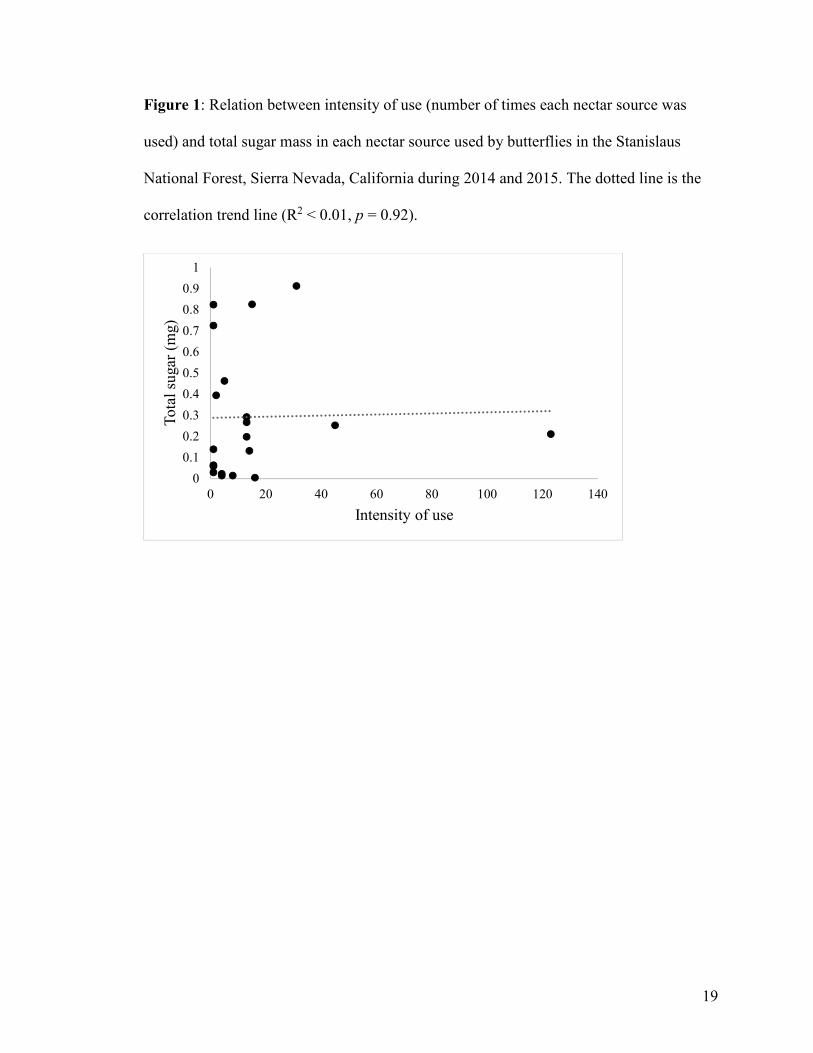
Intensity of use was not associated with the total mass or concentration of sugar

(R2 < 0.01, p = 0.92) (Figure 1), the total amount of sucrose (R2 < 0.01, p = 0.96) (Figure

2), or the relative proportion of sucrose (R2 < 0.01, p = 0.76) (Figure 3). Nor was intensity

of use explained by a combination of total sugar mass, mass of sucrose, and proportion of

sucrose (R2 = 0.02, p= 0.95).

DISCUSSION

On the basis of the results of controlled or laboratory experiments, we anticipated

that as the mass of sugar, mass of sucrose, or relative proportion of sucrose in a given

nectar source increased, intensity of use by butterflies would increase. However, we

found no evidence that intensity of use was associated with sugar mass or concentration,

mass of sucrose, or the relative proportion of sucrose. The lack of correlation between

11

intensity of use and the sugar properties we measured may be attributed to several

factors.

Even if butterflies have preferences related to concentration or composition of

sugar, nectar sources with those attributes may not be available in some locations or time

periods. Different nectar sources are present throughout the flight season. Because

survival or reproduction of many species of butterflies is associated with nectar, a

majority of taxa may be relative generalists with respect to this resource (Scott 1986).

Most of the butterfly species we observed used diverse nectar sources throughout the

season (Table 1). We only analyzed sugar amount in our samples, but other nectar

constituents exist.

Not only sugars but amino acids and water in nectar may affect survival and

reproduction of butterflies (Boggs 1987). Provision of amino acids increased

reproduction in male and female Cenonympha pamphilus and female Araschnia levana

(Mevi-Schutz and Erhardt 2005, Cahenzli and Erhardt 2012, 2013). In controlled

experiments, Pieris rapae preferred solutions with both sugar and amino acids to sugar-

only solutions (Alm et al. 1990). However, male B. philenor preferred solutions with

sugar only to those with both sugar and amino acids (Erhardt 1991). Additionally,

although sucrose, fructose, and glucose are the three main sugars in nectar, other sugars

can be present. It is possible that, when present, these other sugars are used by or attract

butterflies. We recommend that future studies of nectar-source preferences of butterflies,

especially those at the assemblage level, examine amino acid composition and the full

range of sugars.

12

We estimated the amount of sugar in a given floret for each nectar source. Many

factors affect the amount of sugar produced by a floret, including ambient temperature,

time of collection, microclimate, and soil chemistry (Jakobsen and Kristjansson 1994,

Farkas et al. 2012). However, the ratio of sucrose to glucose and fructose in the florets of

a given plant species is relatively constant (Baker and Baker 1982, 1983). We collected

samples at roughly the same time each day, but we could not control for environmental

attributes such as microclimate and soil chemistry, and we did not sample each nectar

source in both years. Additionally, drought may have negative effects on the volume of

nectar produced (Carroll et al. 2001), and our study areas experienced drought conditions

in 2014 and 2015. In non-drought years, the volume of nectar produced may be higher,

although the concentrations of sugars in nectar should remain constant (Carroll et al.

2001). We expected that intensity of use would be greater between sugar concentrations

of 30-50 mg/ml. However, the concentrations in our sugar solutions never exceeded 50

mg/ml, and we found no relation between intensity of use and concentration.

Our response variable was related to use, not preference. In part because we

surveyed transects over a relatively large area, not all nectar sources were available to all

species of butterflies in all locations. Moreover, the period of our observations was brief

relative to the flight period of an individual or species. We observed the greatest number

of individuals feeding on the nectar source for which we recorded the greatest number of

florets, Acmispon nevadensis, which was present on eight of our 12 transects. However,

the species on which we observed the second-greatest number of individuals feeding,

Calyptridium umbellatum, was present on two transects. A few small patches of the

nectar source Apocynum androsaemifolium were present on one transect, but the number

13

of individuals we observed feeding on A. androsaemifolium was greater than the number

we observed feeding on 50% of the nectar sources. By contrast, nectar sources such as

Chamerion angustifolium and C. grandiflora were present and abundant on most

transects, but we observed one individual feeding on each.

Some plant species have many small and dense florets, whereas other species

have one large floret. When florets are dense, insects can take nectar from many florets

without expending much energy on flight, even if the amount of sugar or nectar in each

floret is relatively low (Heinrich and Raven 1972). Some nectar sources in our study area,

such as C. foliolosa and A. nevadensis, were present in patches that included hundreds or

thousands of florets. The density of other nectar sources, such as Drymocallis glandulosa

and Lathyrus nevadensis, was comparatively low.

All of the nectar sources in our study area were native except T. pratense.

Butterflies may prefer native nectar sources or sugars. For example, in upland prairies in

western Oregon, I. icarioides fenderi densities were not associated with the densities of

native flowering plants, but were strongly associated with the mass of sugars from native

sources (Schultz and Dlugosch 1999). Female I. icarioides fenderi preferred native nectar

sources to non-native nectar sources (Thomas and Schultz 2015). It is possible that

butterflies in our study area selected native nectar sources. However, we noted few non-

native species of flowering plants in the areas that we surveyed. Therefore, butterflies

may have had access only to native species, and their use of these native sources may be

attributable to availability rather than preference. Species richness and abundance of

bumblebees, solitary bees, and lepidoptera were greater in plots in which an invasive

14

non-native source of nectar and pollen (the thistle Carduus acanthoides) was present than

in identical plots in which it was absent (Russo et al. 2015).

Previous studies of butterfly preferences for different sugars or nectar sources in

controlled or laboratory settings do not represent what is available to species in an

uncontrolled environment. Our field data were inconsistent with expectations based on

data from laboratory and controlled experiments. Butterflies appeared to use any sources

that were available to them, regardless of nectar or sugar mass or composition. Individual

butterfly species may have sugar preferences, but we found no evidence of assemblage-

level patterns. The difference between intensity of sugar use or sugar preferences in the

laboratory and in the field may be explained by individual species’ preferences,

competition for resources, resource availability, or energy requirements. Moreover, the

abundance of nectar-producing plants, and the volume and concentration of nectar, is

thought to peak in the initial years after a fire. Therefore, as time since fire increases, and

as succession progresses, the composition of plants from which butterflies will take

nectar and the attributes of that nectar will change. Longer-term studies of nectar use

from a more-extensive area may reveal species-specific or temporal patterns.

15

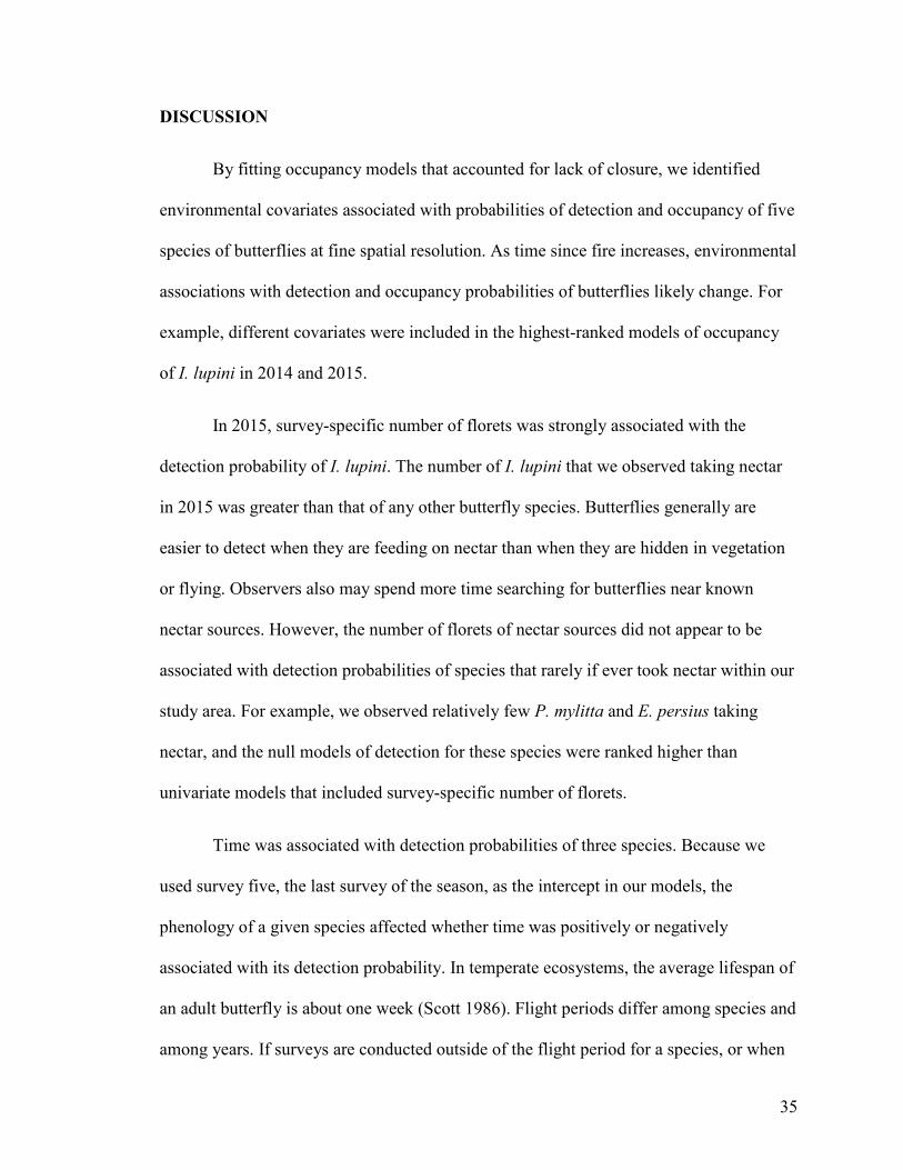
Table 1. Number of butterflies observed during surveys in the Stanislaus National Forest,

Sierra Nevada, California during 2014 and 2015. Taxonomy and nomenclature follow

Pelham (2015).

Number of individuals observed

Species 2014 2015 Number of

observations of feeding

Parnassius clodius 3 3 1 Papilio rutulus 0 5 2 Papilio eurymedon 3 31 3 Papilio multicaudatus 0 1 0 Colias eurytheme 79 482 29 Anthocharis sara 0 3 0 Pieris rapae 0 1 0 Pontia protodice 1 5 1 Pontia occidentalis 0 1 0 Lycaena cupreus 4 1 2 Satyrium californica 0 3 2 Satyrium saepium 0 3 0 Callophrys gryneus 1 14 16 Callophrys augustinus 6 3 6 Strymon melinus 15 10 13 Celastrina ladon 2 16 11 Glaucopsyche piasus 2 23 4 Leptotes marina 0 1 1 Cupido amyntula 2 14 0 Icaricia saepiolus 5 4 0 Icaricia icarioides 17 71 3 Icaricia lupini 198 974 104 Danaus plexippus 5 11 0 Bolora epithore 6 4 0 Speyeria hydaspe 11 28 3 Limenitis lorquini 1 32 1 Adelpha californica 37 23 1 Vanessa virginiensis 0 18 8 Vanessa cardui 90 22 31 Vanessa atalanta 0 1 1 Nymphalis californica 0 1 1 Polygonia gracilis 3 2 0 Junonia coenia 1 189 18 Euphydryas chalcedona 1 1 1 Chlosyne palla 0 1 0

16

Phyciodes mylitta 15 181 25 Coenonympha tullia 2 12 1 Epargyreus clarus 3 4 1 Thorybes pylades 0 1 3 Erynnis propertius 0 1 0 Erynnis persius 6 207 16 Pyrgus communis 2 0 1 Hesperia juba 0 1 0 Polites sonora 0 5 1 Poanes melane 1 1 0 Total 522 2415 312

17

Table 2. Nectar sources, number of butterflies that were observed feeding on those sources in 2014 and 2015, masses (mg) of

constituent sugars, and relative proportion of sucrose. Masses and proportions are averages (± SD) from 5 florets.

Species

Number of observations

of use (2014)

Number of observations

of use (2015) Fructose mass Glucose mass Sucrose mass

Total sugar mass

Proportion sucrose

Acmispon

nevadensis 33 90 0.071 ± 0.040 0.057 ± 0.032 0.083 ± 0.060 0.210 ± 0.127 0.355 ± 0.125

Calyptridium

umbellatum 20 25 0.012 ± 0.009 0.008 ± 0.007 0.002 ± 0.002 0.022 ± 0.017 0.031 ± 0.013

Arnica sp. 0 31 0.463 ± 0.324 0.448 ± 0.276 0.001 ± 0.002 0.913 ± 0.599 0.002 ± 0.003

Ceanothus sp. 1 15 0.002 ± 0.001 0.002 ± 0.001 0.000 ± 0.000 0.004 ± 0.002 0.013 ± 0.025

Chamaebatia

foliolosa 1 14 0.395 ± 0.097 0.382 ± 0.125 0.049 ± 0.008 0.825 ± 0.226 0.061 ± 0.012

Monardella

odoratissima 4 10 0.059 ± 0.042 0.035 ± 0.030 0.037 ± 0.023 0.131 ± 0.089 0.291 ± 0.079

Gilia capitata 3 10 0.110 ± 0.018 0.125 ± 0.011 0.057 ± 0.021 0.292 ± 0.030 0.196 ± 0.065

Dichelostemma

sp. 3 10 0.113 ± 0.049 0.085 ± 0.044 < 0.001 0.198 ± 0.093 < 0.001

Apocynum

androsaemifolium 10 3 0.137 ± 0.149 0.037 ± 0.021 0.092 ± 0.060 0.267 ± 0.217 0365 ± 0.084

18

Trifolium

pratense 1 7 0.008 ± 0.008 0.003 ± 0.003 0.002 ± 0.002 0.014 ± 0.012 0.310 ± 0.387

Drymocallis

glandulosa 1 4 0.270 ± 0.118 0.190 ± 0.083 0.002 ± 0.005 0.463 ± 0.197 0.004 ± 0.007

Anaphalis

margaritacea 0 4 0.012 ± 0.009 0.008 ± 0.007 0.002 ± 0.002 0.022 ± 0.017 0.133 ± 0.066

Erysimum

capitatum 0 4 0.007 ± 0.015 0.004 ± 0.009 0.003 ± 0.007 0.014 ± 0.031 0.248 ± 0.433

Wyethia

angustifolia 0 2 0.145 ± 0.076 0.115 ± 0.061 0.134 ± 0.076 0.394 ± 0.200 0.333 ± 0.088

Eriodictyon

californicum 1 0 0.226 ± 0.060 0.210 ± 0.055 0.289 ± 0.179 0.725 ± 0.275 0.365 ± 0.127

Chamerion

angustifolium 0 1 0.421 ± 0.054 0.276 ± 0.059 0.127 ± 0.043 0.824 ± 0.074 0.157 ± 0.059

Prunella vulgaris 0 1 0.029 ± 0.011 0.021 ± 0.012 0.014 ± 0.002 0.063 ± 0.024 0.241 ± 0.102

Lathyrus

nevadensis 0 1 0.070 ± 0.097 0.035 ± 0.047 0.033 ± 0.066 0.139 ± 0.180 0.114 ± 0.190

Achillea

millefolium 0 1 0.017 ± 0.007 0.010 ± 0.005 0.003 ± 0.002 0.029 ± 0.013 0.094 ± 0.042

Collomia

grandiflora 0 1 0.016 ± 0.009 0.016 ± 0.011 0.027 ± 0.023 0.059 ± 0.043 0.414 ± 0.091

Total 78 234

19

Figure 1: Relation between intensity of use (number of times each nectar source was

used) and total sugar mass in each nectar source used by butterflies in the Stanislaus

National Forest, Sierra Nevada, California during 2014 and 2015. The dotted line is the

correlation trend line (R2 < 0.01, p = 0.92).

0

0.1

0.2

0.3

0.4

0.5

0.6

0.7

0.8

0.9

1

0 20 40 60 80 100 120 140

Tota

l sug

ar (

mg)

Intensity of use

20

Figure 2: Relation between intensity of use (number of times each nectar source was

used) and the total sucrose mass in each nectar source used by butterflies in the Stanislaus

National Forest, Sierra Nevada, California during 2014 and 2015. The dotted line is the

correlation trend line (R2 < 0.01, p = 0.96).

0

0.05

0.1

0.15

0.2

0.25

0.3

0.35

0 20 40 60 80 100 120 140

Suc

rose

mas

s (m

g)

Intensity of use

21

Figure 3: Relation between intensity of use (number of times each nectar source was

used) and proportion of sucrose to total sugar amount in each nectar source used by

butterflies in the Stanislaus National Forest, Sierra Nevada, California during 2014 and

2015. The dotted line is the correlation trend line (R2 < 0.01, p = 0.76).

0.00

0.05

0.10

0.15

0.20

0.25

0.30

0.35

0.40

0.45

0 20 40 60 80 100 120 140

Pro

port

ion

of s

ugar

tha

t is

sucr

ose

Intensity of use

22

CHAPTER 2

Environmental associations with post-fire butterfly occupancy in

the Sierra Nevada, California

23

INTRODUCTION

Fire affects environmental attributes associated with the distribution, abundance,

and reproduction of butterflies, including nectar availability and quality. Adults of many

species of butterflies feed exclusively on nectar, and availability of nectar affects the

population sizes or fecundity of certain species (Murphy et al. 1983, Boggs and Ross

1993, Schultz and Dlugosch 1999). Prescribed fire has been used to increase the

abundance of nectar sources used by butterflies. For example, the abundance of nectar

sources for Lycaeides melissa samuelis, a subspecies listed as endangered under the US

Endangered Species Act, increased after a prescribed fire in Wisconsin, USA (King

2003). In forests of eastern Texas, USA, the abundances of nectar sources used by

butterflies were greatest in areas maintained by prescribed fire (Rudolph and Ely 2000).

Abundance and species richness of butterflies also respond to fire. For example,

following fires in riparian areas within coniferous forests in Oregon and California, USA,

the number of butterflies in burned areas was two to three times greater than the number

in comparable areas that were not burned (Huntzinger 2003). However, the effects of fire

on butterfly occupancy (the probability that a given site is occupied by a given species;

MacKenzie et al. 2002), and on environmental attributes that are associated with butterfly

occupancy, are largely unknown.

Occupancy is relevant to both population monitoring and assessment of habitat

associations. Although estimates of abundance are more-informative measures of

population status than estimates of occupancy, collection of the data necessary to

estimate abundance generally requires more time and money than collection of

occurrence data (MacKenzie et al 2004). Therefore, estimation of abundance may not be

24

feasible for many studies. Because models of occupancy do not require individuals to be

marked or recaptured, they can be applied to animals that occur at low densities, or when

capturing animals is not practical. It is possible that environmental factors that are

associated with occupancy of a species also could be associated with that species’

abundance.

Effective modeling of occupancy depends on whether five assumptions are met

or, if violated, overcome: occupancy probability remains constant, or changes in

probability of occupancy are accurately modeled; probability of detection remains

constant, or changes in probability of detection are accurately modeled; detections of

individuals at each site are independent; species are not falsely detected; and occupancy

status does not change among surveys (closure) (MacKenzie et al. 2002). Application of

occupancy models to multiple species of butterflies that were sampled simultaneously is

complicated by movements of butterflies between surveys (Hayes et al. 2015) and by

taxonomic, temporal, and spatial variation in phenology. In these cases, individual

species often do not meet the assumption of closure. Previous authors have addressed

violations of this assumption by modeling individual broods of multivoltine species

(Pellet 2007) or by limiting analyses to known flight periods (van Strien et al. 2011).

More recently, butterfly occupancy has been estimated with models that relax the

assumption of closure by allowing for a single entry and exit of the species from each

sampling location (Kendall et al. 2013, Roth et al. 2014, Fleishman et al. in review).

Environmental covariates can be added to these models to explore whether they are

associated with probabilities of detection and occupancy.

25

We examined the extent to which butterfly occupancy and abundance in the first

two years following the Rim Fire, one of the largest fires in California since accurate fire

records for that region have been maintained (1932–present), were associated with

environmental attributes that were known or hypothesized to be affected strongly by the

fire. The Rim Fire burned on the west slope of the Sierra Nevada from August through

October 2013 and encompassed more than 1040 km2 (257,000 acres) of public and

private land (USFS 2014). We also tested whether variation in the environmental

attributes that we included in models of butterfly occupancy and abundance was

explained by local differences in fire severity. To our knowledge, this is the first study of

post-fire butterfly occupancy, and the first to compare the effects of environmental

attributes on both butterfly occupancy and abundance.

METHODS

Field Methods

We collected data within the Rim Fire boundary on the Groveland Ranger District

of the Stanislaus National Forest (Tuolumne County, California). The vegetation in the

areas in which we worked is classified as Sierran yellow pine forest and Sierran montane

forest (Miksicek et al. 1996). These forests are dominated by ponderosa pine (Pinus

ponderosa), white fir (Abies concolor), Douglas fir (Pseudotsuga menziesii), sugar pine

(P. lambertiana), incense cedar (Calocedrus decurrens), and black oak (Quercus

kelloggii). Understory species include manzanita (Arctostaphylos spp.), buckbrush

(Ceanothus spp.), mountain misery (Chamaebatia foliolosa), chinquapin (Castanopsis

sempervirens), and various berries (Miksicek et al. 1996).

26

Random selection of sampling locations was not possible due to steep topography,

the lack of roads, and limited time available for travel. In 2014, we established eight 300-

500 m transects along which pre-fire vegetation composition and structure appeared to

have been homogenous. We established an additional four transects within the same

range of lengths in 2015. Transect length varied because in some cases we could not

locate 500 m with apparently homogenous pre-fire vegetation composition and structure.

Transects were placed along established two tracks and roads. The elevation of each

transect ranged from approximately 1350 to 1450 m. In all but one case, the endpoints of

different transects were separated by ≥ 100 m. The maximum linear distance between

transects was approximately 24 km. We sampled each transect that was established in

2014 five times during June and July 2014 and we sampled all transects five times from

May through July 2015, which encompassed the majority of the butterfly flight seasons in

those years. We divided each transect into 20-m segments, which were the sample units

for analysis. During each survey, an observer walked along the transect and identified

each butterfly observed within 10 m on either side (Pollard and Yates 1993). We noted

whether each butterfly was taking nectar, and, if so, the species on which it was feeding.

In some cases, the same individual was observed taking nectar from more than one plant

species. We estimated abundance as the total number of individuals of each species that

we observed during the season. It is possible that a small number of individuals were

recorded on more than one survey, but we considered this situation unlikely given the lag

time between surveys.

We surveyed vegetation along each transect within one day of each butterfly

survey, except in one case, when we conducted vegetation surveys 9 days after butterfly

27

surveys for a subset of the transects due to inclement weather. During each survey, we

used a random number generator to select 1 m2 in each 20-m segment for fine-resolution

vegetation sampling. Within that 1-m2, we used a concave spherical densiometer to

measure the percentage of canopy cover, visually estimated the percentage of live ground

cover, identified all known or potential nectar sources, and counted the number of florets

of each nectar source.

For each plant species on which we observed adult butterflies feeding, we

collected from multiple plants a total of five florets that showed no signs of senescence.

We covered each floret overnight with a fine-mesh cloth bag, secured with a rubber band,

to prevent feeding by insects and to allow nectar to regenerate following any previous

feeding (Bentley and Ellas 1983, Morrant et al. 2009). We collected the florets during the

following afternoon. We placed each floret in a 30 ml plastic vial with 2 ml of distilled

water and shook the vial for 60 sec to wash the nectar from the floret (Grünfeld et al.

1989, Morrant et al. 2009). We maintained the samples on ice (typically for less than a

week) and then transferred the samples to a -80ºC freezer.

We used high performance liquid chromatography-mass spectrometry to quantify

the masses (mg) of glucose, fructose, and sucrose for all plant species from which we

collected florets. In most cases, we analyzed each of the five samples (florets) from each

nectar source. In a small number of cases, we analyzed four rather than five samples due

to improper handling or storage of one sample. We multiplied the mean mass of sugar

(sum of glucose, fructose, and sucrose) for each nectar source by the number of florets in

each 20-m segment to estimate the mass of sugar available to butterflies in that segment.

Full methods for extraction and estimation of sugar mass are in Chapter 1 (Methods).

28

From the vegetation surveys, we derived six environmental covariates for each

segment. We calculated the survey-specific number of florets and also summed the

number of florets across each season. For each season, we calculated the average canopy

cover, live ground cover, sugar mass, and categorical abundance of florets that serve as

nectar sources. Researchers previously found that detection probabilities and occupancy

of a considerable proportion of butterflies in three ecosystems increased as the categorical

abundance of nectar sources increased (Fleishman et al. in review). Those categorical

estimates were intended to classify abundance along an approximately logarithmic or

semi-logarithmic scale. The estimates were comparable among observers in a given

geographic area (Fleishman and Pavlik unpublished data), but might vary among years

and likely would vary among regions. In this study, we measured abundance of nectar

sources quantitatively, as a continuous variable. Nevertheless, to explore whether

inferences about the strength of associations between occupancy and nectar abundance

depended on the precision with which the latter was assessed, we created post-hoc

categories of abundance of nectar sources (none, low, moderate, and high) on the basis of

our previous field experience. In 2014, we classified segment-level abundances of 1-49,

50-399, and > 399 florets as low, moderate, and high, respectively. In 2015, the

abundance of florets was greater than in 2014, and we classified segment-level

abundances of 1-99, 100-499, and > 499 florets as low, moderate, and high, respectively.

We acknowledge that it would have been preferable to conduct a categorical assessment

in the field, but felt the rough comparison was worthwhile regardless.

Analysis Methods

29

We used single-season occupancy models with relaxed closure assumptions in

Program MARK (White and Burnham 1999) to estimate occupancy and detection

probabilities (Kendall et al. 2013). The original occupancy model includes two

parameters: ψi, the probability that a given species is present at site i; and pi,t, the

probability that the species is detected at site i at time t, conditional on its presence

(MacKenzie et al. 2002). The occupancy model with relaxed closure assumptions adds

two parameters: βij, the probability that the species enters the site between visits (surveys)

j and j + 1, given that the site is occupied; and dij, the probability that the species exits the

site (and therefore cannot be detected) before visit j + 1, given that the species is present

on visit j (Kendall et al. 2013). We standardized all continuous covariates. We limited

analyses to species with naïve occupancy (i.e., the proportion of sites in which the species

was observed, not accounting for detection probability) ≥ 0.28 and ≤ 0.70 in each year,

and to those that we observed using the transects (e.g., taking nectar, mating, perching).

We used forward model selection to add covariates to models one at a time, and

implemented model selection in two stages: modeling probability of detection and

modeling probability of occupancy. In both stages, we used Akaike’s Information

Criterion adjusted for small sample sizes (AICc) to compare models (Burnham and

Anderson 2002). In the first stage, we evaluated associations between covariates and

probabilities of detection (pij), entry (βij), and departure (dij). We estimated pij as a fixed

effect of visit (i.e., we estimated pij for each of the 5 surveys). We also tested whether the

survey-specific number of florets affected pij estimates. We used survey five as the

intercept in our models. We estimated βij, and dij as linear functions of time. If univariate

models were ranked lower than the null models, the covariates in the univariate models

30

were not retained for further modeling. We fit multivariate models that contained every

possible combination of covariates from the univariate models that were ranked higher

than the null model. We included the highest-ranked model (or, if the AICc value of a

competing model was within two units of our highest-ranked model, the most

parsimonious model) in the second stage of modeling.

In the second stage, we modeled occupancy as a function of five covariates:

number of florets across the season, categorical abundance of nectar, sugar mass, canopy

cover, and live ground cover. We included ground cover in our models because as the

cover of understory vegetation increases, the distribution and abundance of host plants

also may increase. Additionally, ground cover affects microclimatic factors, such as

temperature, that may affect butterflies (Calvert et al. 1986). We included categorical

abundance of nectar in addition to number of florets and sugar mass because the former

was associated with detection and occupancy of many butterfly species in the Chesapeake

Bay Lowlands of eastern Virginia and in the Great Basin of Nevada and California

(Fleishman et al. in review). Moreover, estimation of categorical abundance of nectar

generally requires less time than estimation of abundance as a continuous variable.

Initially, we fit univariate models of occupancy. Because we fit models with three

different measures of nectar abundance (number of florets, categorical abundance, and

sugar mass), we included only the covariate from the highest-ranked univariate model

(or, if the AICc value of a competing model was within two units of our highest-ranked

model, from the most parsimonious model) in our multivariate models. If the null model

had a higher rank than the univariate models, we did not retain the covariates from the

31

univariate models. If multiple univariate models had higher ranks than the null model, we

fit models with every combination of those covariates.

If the 95% confidence interval of the regression coefficient for a given covariate

in the most highly ranked model did not overlap zero, we considered the covariate to be

associated strongly with the response variable. We report occupancy and detection

probabilities from the highest-ranked model for each species. If the AICc value of a

competing model was within two units of our highest-ranked model, we report occupancy

and detection probabilities from the most parsimonious model.

We used univariate, negative binomial generalized linear models to examine the

effects of canopy cover, live ground cover, number of florets, sugar mass, and categorical

abundance of nectar sources on the abundances of the species for which we modeled

occupancy.

We used single-factor, one-way analysis of variance (ANOVA) to examine

relations between soil and vegetation burn severity and canopy cover, live ground cover,

number of florets, and sugar mass in 2014 and 2015. We excluded transects that had been

logged after the 2014 field season from our analysis of canopy cover in 2015 (n = 2). We

used Tukey’s post-hoc tests to quantify pairwise differences between fire severity classes.

During the first survey in 2014, we qualitatively classified the proportion of each segment

that burned (none, some, or all). We used ArcGIS v. 10.3 (ESRI, Redlands, California) to

compare these data with remotely sensed measures of vegetation burn severity from the

US Forest Service’s Rapid Assessment of Vegetation Condition after Wildfire (RAVG)

process (http://www.fs.fed.us/postfirevegcondition/index.shtml). The RAVG

classification generally matched our classification. The RAVG process derives vegetation

32

burn severity by applying a Relative Differenced Normalized Burn Ratio (RdNBR) to

pre-fire and post-fire images from the Landsat Thematic Mapper. Vegetation burn

severity was classified by RAVG as unchanged, low, moderate, or high. We obtained

estimates of soil burn severity from the US Forest Service’s Burned Area Emergency

Response (BAER) team (http://activefiremaps.fs.fed.us/baer/download.php?year=2013).

The BAER team derives soil burn severity by measuring the difference in spectral

reflectivity in pre-fire and post-fire satellite images. Soil burn severity was classified as

unburned or very low, low, moderate, or high. If any of our segments overlapped multiple

severity classes, we assigned the segment to the severity class that covered the majority

of that segment. If multiple severity classes appeared to be equally represented in a

segment, we assigned the segment to the lower severity class.

RESULTS

In 2014, we recorded 1-198 individuals of 29 species of butterflies (Table 1). One

species, Icaricia lupini, met our criteria for modeling occupancy. In 2015, we observed 1-

974 individuals of 44 species of butterflies (Table 1). Five species—Colias eurytheme,

Icaricia lupini, Junonia coenia, Phyciodes mylitta, and Erynnis persius—met our criteria

for modeling occupancy. Naïve estimates of occupancy were 0.63 for C. eurytheme, 0.38

and 0.66 for I. lupini in 2014 and 2015, respectively, 0.52 for J. coenia, 0.44 for P.

mylitta, and 0.28 for E. persius. The number of florets of nectar sources per segment was

83.8 ± 322.6 (mean ± SD) in 2014 and 143.0 ± 341.6 in 2015.

Maximum detection probabilities on a given survey ranged from 0.35 for J.

coenia to 0.81 for I. lupini (2015) and E. persius (Table 2). Time was associated with the

probability of detection of J. coenia, P. mylitta, and E. persius (effect sizes varied among

33

surveys). Survey-specific number of florets was associated with the probability of

detection of I. lupini (0.95) in 2015. No covariates were associated with the probability of

detecting I. lupini in 2014 or C. eurytheme in 2015.

Occupancy ranged from 0.22 (E. persius) to 0.88 (C. eurytheme) (Table 2).

Occupancy of each species was associated with at least one covariate (Table 3). Canopy

cover was negatively associated with occupancy of C. eurytheme, I. lupini, P. mylitta,

and E. persius. Regression coefficients ranged from -1.20 for P. mylitta to -1.81 for C.

eurytheme. Live ground cover was positively associated with occupancy of I. lupini, J.

coenia, and P. mylitta. Regression coefficients ranged from 0.47 (2014) for I. lupini

(2014) to 1.75 for P. mylitta. Number of florets was positively associated with occupancy

of I. lupini (2014; regression coefficient 4.04) and E. persius (1.18). Sugar mass was

positively associated with occupancy of C. eurytheme (regression coefficient 2.23).

Categorical abundance of nectar was not associated with occupancy of any species. The

highest-ranked or most parsimonious models for all species except J. coenia included

multiple covariates (Table 3).

Occupancy models for C. eurytheme and I. lupini (2015) that included sugar mass

were supported more strongly than models that included number of florets or categorical

abundance of nectar. Models for I. lupini (2014), P. mylitta, and E. persius that included

number of florets were supported more strongly than models that included sugar mass or

categorical abundance of nectar. The null model for J. coenia was supported more

strongly than models that included nectar covariates.

Canopy cover was significantly associated with the abundances of C. eurytheme,

I. lupini (2015), P. mylitta, and E. persius (Table 4). Live ground cover was significantly

34

associated with the abundances of all five species (Table 4). Categorical nectar

abundance was significantly associated with the abundances of C. eurytheme, I. lupini

(2015), P. mylitta, and E. persius (Table 4). Number of florets and sugar mass were

significantly associated with the abundances of C. eurytheme, I. lupini (2015), and E.

persius (Table 4).

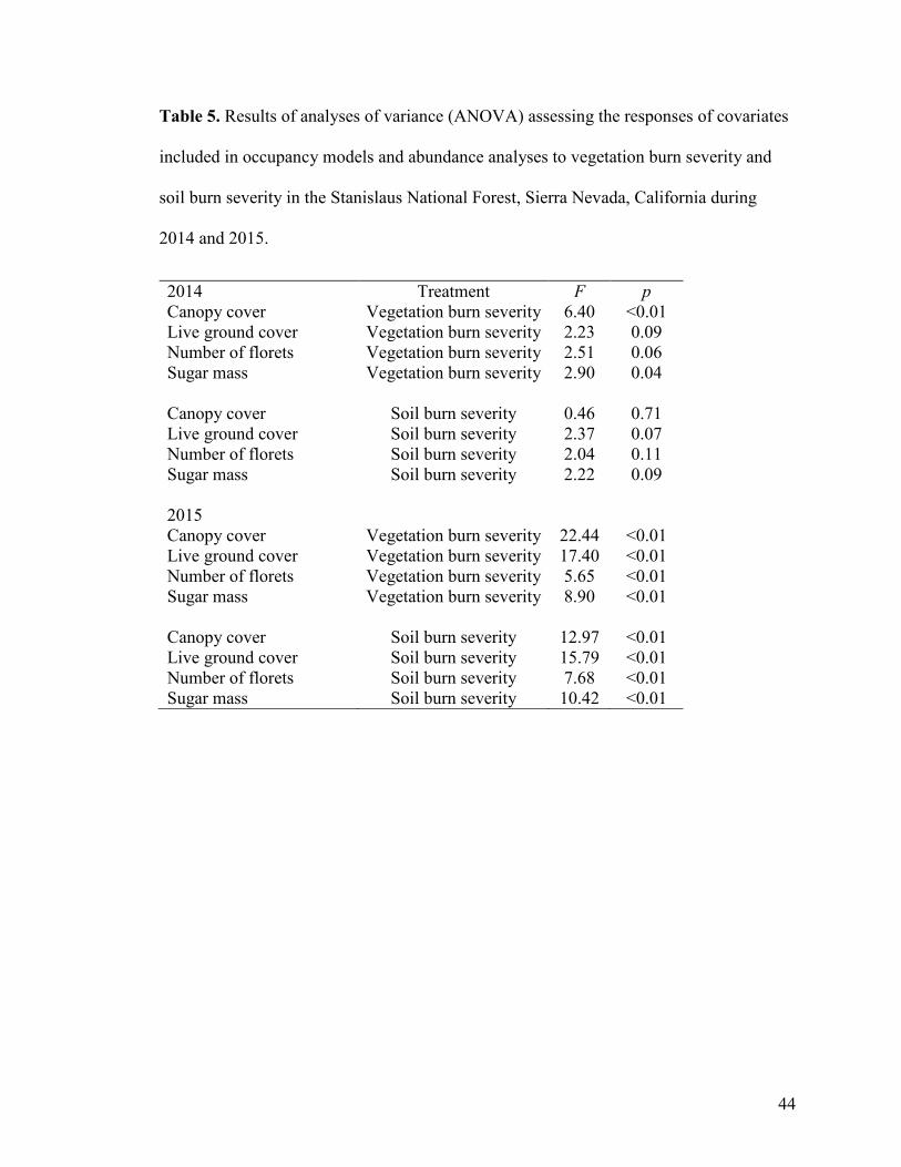
In 2014, canopy cover and sugar mass were significantly associated with

vegetation burn severity (Table 5). Average canopy cover in areas with low, moderate,

and high vegetation burn severity was significantly lower than in unchanged areas

(Tables 6, 8). In 2015, all environmental covariates were significantly associated with

vegetation burn severity (Table 5). Canopy cover decreased significantly as vegetation

burn severity increased (Tables 6, 8). Live ground cover was significantly greater in areas

with moderate or high vegetation burn severity than in unchanged areas or areas with low

vegetation burn severity. Number of florets and sugar mass were significantly greater in

areas with high vegetation burn severity than in unchanged areas or areas with low

vegetation burn severity.

In 2014, no covariates were significantly associated with soil burn severity (Table

5). In 2015, however, all environmental covariates were significantly associated with soil

burn severity. Canopy cover was significantly greater in areas that were unburned or had

very low or low soil burn severity than in areas with moderate soil burn severity (Tables

7, 8). Live ground cover was significantly greater in areas with moderate soil burn

severity than in areas with any other severity level. Number of florets and sugar mass

were significantly greater in areas with moderate soil burn severity than in areas that were

unburned or had very low or low soil burn severity.

35

DISCUSSION

By fitting occupancy models that accounted for lack of closure, we identified

environmental covariates associated with probabilities of detection and occupancy of five

species of butterflies at fine spatial resolution. As time since fire increases, environmental

associations with detection and occupancy probabilities of butterflies likely change. For

example, different covariates were included in the highest-ranked models of occupancy

of I. lupini in 2014 and 2015.

In 2015, survey-specific number of florets was strongly associated with the

detection probability of I. lupini. The number of I. lupini that we observed taking nectar

in 2015 was greater than that of any other butterfly species. Butterflies generally are

easier to detect when they are feeding on nectar than when they are hidden in vegetation

or flying. Observers also may spend more time searching for butterflies near known

nectar sources. However, the number of florets of nectar sources did not appear to be

associated with detection probabilities of species that rarely if ever took nectar within our

study area. For example, we observed relatively few P. mylitta and E. persius taking

nectar, and the null models of detection for these species were ranked higher than

univariate models that included survey-specific number of florets.

Time was associated with detection probabilities of three species. Because we

used survey five, the last survey of the season, as the intercept in our models, the

phenology of a given species affected whether time was positively or negatively

associated with its detection probability. In temperate ecosystems, the average lifespan of

an adult butterfly is about one week (Scott 1986). Flight periods differ among species and

among years. If surveys are conducted outside of the flight period for a species, or when

36

few individuals are present, detection probabilities will be lower than if surveys are

conducted during peak flight periods or when many individuals are present. However, if

the flight period is sufficiently long (e.g., if the species has multiple broods) and

individuals are available for detection throughout the sampling period, the probability of

detection may not change over time. I. lupini and C. eurytheme were present during all

surveys, and probabilities of detection of these species were not associated with time. We

noted temporal changes in the presence and abundance of the three species for which

time was associated with probability of detection.

Live ground cover was positively associated with occupancy of three species. We

observed each of the five species that we modeled laying eggs on plants in the

understory. As noted above, ground cover may be correlated with the distribution and

abundance of host plants and microclimate. Additionally, ground cover may be positively

correlated with the number of florets of nectar sources, although we found a negative

correlation between these two covariates in our study (r = -0.31).

Canopy cover was strongly and negatively associated with occupancy of four

species. Some species of butterflies bask to increase or maintain body temperatures

(Clench 1966). As canopy cover decreases, solar insolation in the understory increases.

Solar insolation may affect butterflies either physiologically (Weiss et al. 1988, 1991) or

indirectly, via responses of host plants, nectar sources, and other plants that provide

shelter or perches in the understory.

We previously included categorical abundance of nectar in occupancy models for

butterflies (Fleishman et al. in review). Our results suggest that continuous measures of

nectar abundance may explain a greater proportion of the variance in probabilities of

37

detection and occupancy than categorical measures. The number of florets often was

more strongly associated with occupancy than abundance classes or sugar mass.

Additionally, the time and cost necessary to estimate sugar mass with high performance

liquid chromatography-mass spectrometry is considerably higher than that necessary to

estimate the number of florets.

Abundances of butterflies increased substantially between the first and second

growing seasons after the Rim Fire. For example, we detected 198 I. lupini in 2014 and

974 in 2015. Canopy cover was associated with both abundance and occupancy of all

species except J. coenia. Live ground cover was associated with the abundances of all

five species and with occupancy of all species except E. persius. Categorical nectar

abundance was not associated with occupancy of any species, but was significantly

associated with the abundances of four species. Number of florets and sugar mass

generally were more strongly associated with abundance than with occupancy of

butterflies.

Fire severity affected values of environmental variables associated with butterfly

occupancy, such as canopy cover and live ground cover. Many plant species that are used

by butterflies are early successional species, and high levels of soil nutrients after the fire

may have supported growth of understory plants (Rice 1993). Our results suggest that

fires of high and moderate severity, or patches in which severity was relatively high, may

stimulate regrowth of understory plants and increase nectar source abundance more than

low-severity fires, while decreasing canopy cover. Butterfly occupancy and abundance

ultimately may be greater in areas in which fire severity was moderate or high than in

areas with low severity fires.

38

Life history traits of butterflies also may affect their spatial distribution or

colonization rates after a fire. J. coenia and C. eurytheme typically travel long distances

as adults (Scott 1986, Fleishman et al. 1997), and species with high vagility may be able

to colonize severely burned areas more quickly than species with low vagility. However,

we recorded numerous species with low vagility in areas with high burn severity in the

first growing season after the Rim Fire. I. lupini, the only species with sufficiently high

naïve occupancy in 2014 to facilitate occupancy analysis, typically does not move large

distances as an adult (Scott 1986, Fleishman et al. 1997). The distance from our transects

to the nearest unburned patches was greater than the reported vagility of this species. Our

data and observations suggest that some adults or larvae can survive high-severity fire,

are capable of moving longer distances than reported, or move in association with smoke

plumes. For example, some species of beetles can detect smoke from fires and use these

signals as cues for dispersal (Schütz et al. 1999). However, this behavior has not been

observed in butterflies.

Environmental attributes other than the abundance of host plants and nectar

sources were associated with occupancy of butterflies after a major fire in the Sierra

Nevada, California. Some of these environmental attributes also were associated with

abundances of butterflies, although the consistency of associations varied among species.

Vegetation and soil burn severity, in turn, affected the environmental attributes that were

associated with occupancy and abundance. Understanding how vegetation and soil burn

severity affects environmental attributes that are associated with butterfly occupancy and

abundance may inform strategies for managing these species with prescribed fire or

following wildfire.

39

Table 1. Number of butterflies observed during surveys in the Stanislaus National Forest,

Sierra Nevada, California during 2014 and 2015. Taxonomy and nomenclature follow

Pelham (2015).

Number of individuals observed Species 2014 2015

Parnassius clodius 3 3 Papilio rutulus 0 5

Papilio eurymedon 3 31 Papilio multicaudatus 0 1

Colias eurytheme 79 482 Anthocharis sara 0 3

Pieris rapae 0 1 Pontia protodice 1 5

Pontia occidentalis 0 1 Lycaena cupreus 4 1

Satyrium californica 0 3 Satyrium saepium 0 3

Callophrys gryneus 1 14 Callophrys augustinus 6 3

Strymon melinus 15 10 Celastrina ladon 2 16

Glaucopsyche piasus 2 23 Leptotes marina 0 1 Cupido amyntula 2 14 Icaricia saepiolus 5 4 Icaricia icarioides 17 71

Icaricia lupini 198 974 Danaus plexippus 5 11 Bolora epithore 6 4

Speyeria hydaspe 11 28 Limenitis lorquini 1 32

Adelpha californica 37 23 Vanessa virginiensis 0 18

Vanessa cardui 90 22 Vanessa atalanta 0 1

Nymphalis californica 0 1 Polygonia gracilis 3 2

Junonia coenia 1 189 Euphydryas chalcedona 1 1

Chlosyne palla 0 1 Phyciodes mylitta 15 181

40

Coenonympha tullia 2 12 Epargyreus clarus 3 4 Thorybes pylades 0 1

Erynnis propertius 0 1 Erynnis persius 6 207

Pyrgus communis 2 0 Hesperia juba 0 1 Polites sonora 0 5 Poanes melane 1 1

Total 522 2415

41

Table 2. Probabilities of detection and occupancy for butterflies in the Stanislaus

National Forest, Sierra Nevada, California in 2014 and 2015. 95% confidence intervals

are shown in parentheses.

Species and year Detection Occupancy Colias eurytheme (2015) 0.71 (0.63–0.78) 0.88 (0.73–0.95)

Icaricia lupini (2014) 0.78 (0.53–0.91) 0.58 (0.41–0.73) Icaricia lupini (2015) 0.81 (0.73–0.87) 0.78 (0.69–0.85) Junonia coenia (2015)

0.35 (0.27–0.45) 0.85 (0.46–0.97) Phyciodes mylitta (2015)

0.67 (0.33–0.90) 0.83 (0.45–0.96) Erynnis persius (2015)

0.73 (0.54–0.86) 0.22 (0.15–0.32)

42

Table 3. Estimates of regression coefficients in the highest ranked or most parsimonious models of occupancy of butterflies in the

Stanislaus National Forest, Sierra Nevada, California during 2014 and 2015. 95% confidence intervals are shown in parentheses.

Species and year Canopy cover Live ground cover

Categorical abundance of nectar

Number of florets Sugar mass

Colias eurytheme (2015) -1.81 (-2.57 – -1.05) 2.23 (0.32–4.14) Icaricia lupini (2014) 0.47 (0.07–0.86) 4.04 (1.34–6.74) Icaricia lupini (2015) -1.30 (-1.83 – -0.78) 0.72 (0.28–1.16) Junonia coenia (2015) 1.62 (0.21–3.04)

Phyciodes mylitta (2015) -1.20 (-2.12 – -0.28) 1.75 (0.27–3.23) Erynnis persius (2015) -1.76 (-2.26 – -1.25) 1.18 (0.20–2.16)

43

Table 4. Relations between environmental covariates and abundances of butterflies in the Stanislaus National Forest, Sierra Nevada,

California during 2014 and 2015. p-values derived from negative binomial generalized linear models.

Species and year Canopy cover Live ground cover Categorical

abundance of nectar Number of

florets Sugar mass Colias eurytheme (2015) < 0.01 < 0.01 < 0.01 < 0.01 < 0.01

Icaricia lupini (2014) 0.20 < 0.01 0.06 0.48 0.60 Icaricia lupini (2015) < 0.01 < 0.01 < 0.01 < 0.01 < 0.01 Junonia coenia (2015) 0.17 < 0.01 0.40 0.22 0.97

Phyciodes mylitta (2015) < 0.01 < 0.01 < 0.01 0.13 0.14 Erynnis persius (2015) < 0.01 0.01 0.01 < 0.01 < 0.01

44

Table 5. Results of analyses of variance (ANOVA) assessing the responses of covariates

included in occupancy models and abundance analyses to vegetation burn severity and

soil burn severity in the Stanislaus National Forest, Sierra Nevada, California during

2014 and 2015.

2014 Treatment F p Canopy cover Vegetation burn severity 6.40 <0.01 Live ground cover Vegetation burn severity 2.23 0.09 Number of florets Vegetation burn severity 2.51 0.06 Sugar mass Vegetation burn severity 2.90 0.04 Canopy cover Soil burn severity 0.46 0.71 Live ground cover Soil burn severity 2.37 0.07 Number of florets Soil burn severity 2.04 0.11 Sugar mass Soil burn severity 2.22 0.09 2015 Canopy cover Vegetation burn severity 22.44 <0.01 Live ground cover Vegetation burn severity 17.40 <0.01 Number of florets Vegetation burn severity 5.65 <0.01 Sugar mass Vegetation burn severity 8.90 <0.01 Canopy cover Soil burn severity 12.97 <0.01 Live ground cover Soil burn severity 15.79 <0.01 Number of florets Soil burn severity 7.68 <0.01 Sugar mass Soil burn severity 10.42 <0.01

45

Table 6. p-values derived from Tukey’s pairwise comparisons between vegetation burn severity classes and environmental covariates

in the Stanislaus National Forest, Sierra Nevada, California during 2014 and 2015.

2014 2015 Vegetation burn severity classes Canopy cover Sugar mass Canopy cover Live ground cover Number of florets Sugar mass Unchanged : Low 0.01 ~1.00 0.02 0.52 0.83 0.80 Unchanged : Moderate

<0.01 0.27 0.00

0.01 0.27 0.13

Unchanged : High 0.01 0.38 0.00 0.00 0.01 0.00 Low : Moderate 0.32 0.10 0.00 0.04 0.45 0.21 Low : High 0.99 0.12 0.00 0.00 0.00 0.00 Moderate : High 0.21 0.99 0.14 0.09 0.53 0.34

46

Table 7. p-values derived from Tukey’s pairwise comparisons between soil burn severity classes and environmental covariates in the

Stanislaus National Forest, Sierra Nevada, California during 2015.

2015

Soil burn severity classes Canopy cover Live ground cover Number of florets

Sugar mass

Unburned / very low : Low 0.90 0.99 0.99 ~1.00

Unburned / very low : Moderate 0.00 0.00 0.02 0.00

Unburned / very low : High 0.65 0.99 0.52 0.17

Low : Moderate 0.00 0.00 0.00 0.00

Low : High 0.49 0.99 0.31 0.13

Moderate : High 0.97 0.01 0.93 0.97

47

Table 8. Average values (± SE) of environmental covariates associated with different vegetation and soil burn severity classes for

statistically significant ANOVAs in 2014 and 2015 (see Table 5).

Severity class

Covariate Treatment

Unchanged (vegetation) or

Unburned / very low (soil) Low Moderate High

2014 Canopy cover (percent) Vegetation burn severity 88.51 ± 2.52 69.60 ± 2.96 61.86 ± 3.95 70.97 ± 2.80

Sugar mass (mg) Vegetation burn severity 0.57 ± 0.52 2.97 ± 1.07 37.23 ± 22.90 32.15 ± 8.29

2015 Canopy cover (percent) Vegetation burn severity 87.57 ± 1.90 71.91 ± 2.16 56.82 ± 3.78 46.46 ± 4.17

Live ground cover (percent) Vegetation burn severity 28.24 ± 3.56 33.99 ± 1.57 42.79 ± 2.61 50.73 ± 2.23 Number of florets Vegetation burn severity 6.22 ± 2.14 71.31 ± 17.28 162.26 ± 61.56 245.72 ± 47.50 Sugar mass (mg) Vegetation burn severity 3.71 ± 1.48 18.85 ± 3.07 44.74 ± 13.03 67.06 ± 10.64

Canopy cover (percent) Soil burn severity 68.01 ± 4.42 71.18 ± 1.93 45.20 ± 4.26 51.39 ± 20.74

Live ground cover (percent) Soil burn severity 36.47 ± 2.87 35.37 ± 1.54 52.89 ± 2.35 36.9 ± 4.39 Number of florets Soil burn severity 82.76 ± 27.89 65.22 ± 18.18 283.92 ± 57.76 225.21 ± 89.85 Sugar mass (mg) Soil burn severity 18.11 ± 5.22 20.74 ± 3.81 74.15 ± 12.73 65.53 ± 20.19

48

LITERATURE CITED

Alm, J., T.E. Ohnmeiss, J. Lanza, and L. Vriesenga. 1990. Preference of cabbage white butterflies and honey bees for nectar that contains amino acids. Oecologia 84:53–57.

Baker, H.G. and I. Baker. 1982. Chemical constituents of nectar in relation to pollination mechanisms and phylogeny. Pages 131–171 in M.H. Nitecki, editor. Biochemical aspects of evolutionary biology. University of Chicago Press, Chicago, Illinois.

Baker, H.G. and I. Baker. 1983. Floral nectar sugar constituents in relation to pollinator type. Pages 117–141 in C.E. Jones and R.J. Little, editors. Handbook of experimental pollination biology. Van Nostrand Reinhold, New York, New York.

Bentley, B. and T. Ellas. 1983. The biology of nectaries. Columbia University Press, New York, New York.

Boggs, C.L. 1987. Ecology of nectar and pollen feeding in Lepidoptera. Pages 369-391 in F. Slansky Jr. and J.G. Rodriguez, editors. Nutritional ecology of insects, mites and spiders and related invertebrates. John Wiley and Sons, New York.

Boggs, C.L. 1988. Rates of nectar feeding in butterflies: effects of sex, size, age and nectar concentration. Functional Ecology 2:289–295.

Boggs, C.L. and C.L. Ross. 1993. The effect of adult food limitation on life history traits in Speyeria mormonia (Lepidoptera: Nymphalidae). Ecology 74:433–441.

Burnham, K.P. and D.R. Anderson. 2002. Model selection and multimodel inference: a practical information–theoretic approach. Springer–Verlag, New York.

Cahenzli, F. and A. Erhardt. 2012. Enhancing offspring quality or quantity? Different ways for using nectar amino acids in female butterflies. Oecologia 169:1005–1014.

Cahenzli, F. and A. Erhardt. 2013. Nectar amino acids enhance reproduction in male butterflies. Oecologia 171:197–205.

Calvert, W.H., Hyatt, M., and N.P.M. Villaseñor. 1986. The effects of understory vegetation on the survival of overwintering monarch butterflies, (Danaus plexippus L.) in Mexico. Acta Zoologica Mexicana 18:1-17.

Carroll, A.B., S.G. Pallardy, and C. Galen. 2001. Drought stress, plant water status, and floral trait expression in fireweed, Epilobium angustifolium (Onagraceae). American Journal of Botany 88:438–446.

Clench, H.K. 1966. Behavioral thermoregulation in butterflies. Ecology 47:1021–1034.

Curtis, R. J., T.M. Brereton, R.L.H Dennis, C. Carbone, and N.J.B Isaac. 2015. Butterfly abundance is determined by food availability and is mediated by species traits. Journal of Applied Ecology. doi: 10.1111/1365-2664.12523

49

Erhardt, A. 1991. Nectar sugar and amino acid preferences of Battus philenor (Lepidoptera, Papilonidae). Ecological Entomology 16:425–434.

Erhardt, A. 1992. Preferences and non-preferences for nectar constituents in Ornithoptera Priamus poseidon (Lepidoptera, Papilionidae). Oecologia 90:581–585.

Farkas, Á., R. Molnár, T. Morschhauser, and I. Hahn. 2012. Variation in nectar volume and sugar concentration of Allium ursinum L. ssp. ucrainicum in three habitats. The Scientific World Journal 2012:1–7.

Fleishman, E., G.T. Austin, and D.D. Murphy. 1997. Natural history and biogeography of the butterflies of the Toiyabe Range, Nevada (Lepidoptera: Papilionoidea). Holarctic Lepidoptera 4:1–18.

Grünfeld, E., C. Vincent, and D. Bagnara. 1989. High-performance liquid chromatography analysis of nectar and pollen of strawberry flowers. Journal of Agriculture and Food Chemistry 37:290–294.

Hayes, D.B. and M.J. Monfils. 2015. Occupancy modeling of bird point counts: implications of mobile animals. Journal of Wildlife Management 79:1361–1368.

Heinrich, B. and P.H. Raven. 1972. Energetics and pollination ecology: the energetics of pollinators may have wide implications in floral biology and community ecology. Science 176:597–602.

Huntzinger, M. 2003. Effects of fire management practices on butterfly diversity in the forested western United States. Biological Conservation 113:1–12.

Jakobsen, H.B. and K. Kritjansson. 1994. Influence of temperature and floret age on nectar secretion in Trifolium repens L. Annals of Botany 74:327-334.

Kendall, W.L., J.E. Hines, J.D. Nichols, and E.H. Campbell Grant. 2013. Relaxing the closure assumption in occupancy models: staggered arrival and departure times. Ecology 94:610–617.

King, R.S. 2003. Habitat management for the Karner blue butterfly (Lycaeides melissa

samuelis), evaluating the short-term consequences. Ecological Restoration 21:101–106.

MacKenzie, D.I., J.D. Nichols, G.B. Lachman, S. Droege, J.A. Royle, K.P. Pollock, L.L. Bailey, and C.A. Langtimm. 2002. Estimating site occupancy rates when detection probabilities are less than one. Ecology 83:2248–2255.

MacKenzie, D.I., J.A. Royle, J.A. Brown, and J.D. Nichols. 2004. Occupancy estimation and modeling for rare and elusive populations. Pages 149–172 in W.L. Thompson, editor. Sampling rare or elusive species: concepts, designs, and

50

techniques for estimating population parameters. Island Press, Washington, D.C., USA.

May, P.G. 1985. Nectar uptake rates and optimal nectar concentrations in two butterfly species. Oecologia 66:381–386.

Mevi-Schutz, J. and A. Erhardt. 2005. Amino acids in nectar enhance butterfly fecundity: a long-awaited link. The American Naturalist 165:411–419.

Miksicek, C., K. Roper, D. Simons, J. Farquhar, K Loeffler, J. Hall, T.L. Jackson, and R.J. Jackson. 1996. Overview of the prehistory of the Stanislaus National Forest. http://www.fs.usda.gov/Internet/FSE_DOCUMENTS/fsm91_057359.pdf

Morrant, D.S., R. Schumann, and S. Petit. 2009. Field methods for sampling and storing nectar from flowers with low nectar volumes. Annals of Botany 103:533–542.

Murphy, D.D., A.E Launer, and P.R. Ehrlich. 1983. The role of adult feeding in egg production and population dynamics of the checkerspot butterfly Euphydryas editha. Oecologia 56:257–263.

Neter, J., M.H. Kutner, C.J. Nachtsheim, and W. Wasserman. 1996. Applied linear statistical models. 4th edition. McGraw-Hill, Chicago, Illinois.

Northrup, J.M., M.B. Hooten, C.R. Anderson Jr., and G. Wittemyer. 2013. Practical guidance on characterizing availability in resource selection functions under a use-availability design. Ecology 94:1456–1463.

O’Brien, D.M., C.L. Boggs, and M.L. Fogel. 2004. Making eggs from nectar: the role of life history and dietary carbon turnover in butterfly reproductive resource allocation. Oikos 105:279–291.

Pelham, J.P. 2015. A catalogue of the butterflies of the United States and Canada. http://butterfliesofamerica.com/US-Can-Cat.htm, accessed October 2015.

Pellet, J., E. Fleishman, D.S. Dobkin, A. Gander, and D.D. Murphy. 2007. An empirical evaluation of the area and isolation paradigm of metapopulation dynamics. Biological Conservation 136:483–495.

Pivnick, K.A. and J.N. McNeil. 1985. Effects of nectar concentration on butterfly feeding: measured feeding rates for Thymelicus lineola (Lepidoptera: Hesperiidae) and a general feeding model for adult Lepidoptera. Oecologia 66:226–237.

Pollard, E. and T.J. Yates. 1993. Monitoring butterflies for ecology and conservation. Chapman and Hall, London.

51

Potts, S.G., B. Vulliamy, A. Dafni, G. Ne’eman, C. O’Toole, S. Roberts, and P. Willmer. 2003. Response of plant-pollinator communities to fire: changes in diversity, abundance and floral reward structure. Oikos 101:103–112.

Pyke, G.H., H.R. Pulliam, and E.L. Charnov. 1977. Optimal foraging: a selective review of theory and tests. Quarterly Review of Biology 52:137–154.

Rice, S.K. 1993. Vegetation establishment in post-fire Adenostoma chaparral in relation to fine-scale pattern in fire intensity and soil nutrients. Journal of Vegetation Science 4:115–124.

Roth, T., N. Strebel, and V. Amrhein. 2014. Estimating unbiased phenological trends by adapting site-occupancy models. Ecology 95:2144–2154.

Rudolph, D.C. and C.A. Ely. 2000. The influence of fire on lepidopteran abundance and community structure in forested habitats of eastern Texas. Texas Journal of Science 52:127–138.

Russo, L., C. Nichol, and K. Shea. 2015. Pollinator floral provisioning by a plant invader: quantifying beneficial effects of a detrimental species. Diversity and Distributions. doi: 10.1111/ddi.12397

Rusterholz, H.P. and A. Erhardt. 1997. Preferences for nectar sugars in the peacock butterfly, Inachis io. Ecological Entomology 22:220–224.

Schultz, C.B. and K.M. Dlugosch. 1999. Nectar and hostplant scarcity limit populations of an endangered Oregon butterfly. Oecologia 119:231–238.

Schütz, S., Weissbecker, B., Hummel, H., Apel, K.H., Schmitz, H., and H. Bleckmann. 1999. Insect antenna as a smoke detector. Nature 398:298:299.

Scott, J.A. 1986. The butterflies of North America. Stanford University Press, Stanford, California.

Thomas, R.C. and Schultz, C.B. 2015. Resource selection in an endangered butterfly: females select native nectar species. Journal of Wildlife Management. doi: 10.1002/jwmg.987

USDA Forest Service (USFS). 2014. Rim Fire recovery (43033): Environmental Impact Statement. http://a123.g.akamai.net/7/123/11558/abc123/forestservic.download.akamai.com/11558/www/nepa/97293_FSPLT3_2325973.pdf

Watt, W.B., P.C. Hoch, and S.G. Mills. 1974. Nectar resource use by Colias butterflies - chemical and visual aspects. Oecologia 14:353–374.

52

Weiss, S.B., D.D. Murphy, and R.R. White. 1988. Sun, slope, and butterflies: topographic determinants of habitat quality for Euphydryas editha. Ecology 69:1486–1496.

Weiss, S.B., Rich, P.M., Murphy, D.D., Calvert, W.H., and P.R. Ehrlich. 1991. Forest canopy structure at overwintering monarch butterfly sites: measurements with hemispherical photography. Conservation Biology 5:165–175.

White, G.C., and K.P. Burnham. 1999. Program MARK: survival estimation from populations of marked animals. Bird Study 46 Supplement:120–138.

53

APPENDIX A: Occupancy models for butterflies in the Stanislaus National Forest,

Sierra Nevada, California during 2014 and 2015. Covariates included in models of

occupancy (ψ), entry (β), departure (d), and detection (p) were time (survey number; T),

survey-specific number of florets (florS), live ground cover (live), canopy cover

(canopy), seasonal number of florets (flor), sugar mass (sugar), and categorical

abundance of nectar (nectar).

Table A1.1. Associations between covariates and probabilities of detection, entry, and

departure of Junonia coenia in the Stanislaus National Forest, Sierra Nevada, California

during 2015. Occupancy was held constant.

Model AICc ΔAICc Number of parameters ψ (.) β (T) d (T) p (florS+T) 1009.76 0.00 11 ψ (.) β (T) d (T) p (T) 1010.88 1.12 10 ψ (.) β (.) d (.) p (T) 1012.32 2.56 8 ψ (.) β (.) d (.) p (florS+T) 1012.82 3.06 9 ψ (.) β (T) d (T) p (florS) 1025.41 15.65 7 ψ (.) β (T) d (T) p (.) 1027.13 17.37 6 ψ (.) β (.) d (.) p (florS) 1050.03 40.27 5 ψ (.) β (.) d (.) p (.) 1054.13 44.37 4

54

Table A1.2. Associations between covariates and occupancy of Junonia coenia in the

Stanislaus National Forest, Sierra Nevada, California during 2015. We used the highest-

ranked model, or, if the AICc value of a competing model was within two units of our

highest-ranked model, the most parsimonious model, from the first model section step in

this step of model selection.

Model AICc ΔAICc Number of parameters ψ (live) β (T) d (T) p (T) 987.66 0.00 10 ψ (canopy+live) β (T) d (T) p (T) 990.74 3.08 12 ψ (flor+live) β (T) d (T) p (T) 991.99 4.33 12 ψ (canopy+live+flor) β (T) d (T) p (T) 992.89 5.23 13 ψ (canopy) β (T) d (T) p (T) 995.74 8.08 9 ψ (canopy+flor) β (T) d (T) p (T) 1002.17 14.51 12 ψ (flor) β (T) d (T) p (T) 1010.87 23.21 11 ψ (.) β (T) d (T) p (T) 1010.88 23.22 10 ψ (sugar) β (T) d (T) p (T) 1012.48 24.82 11 ψ (nectar) β (T) d (T) p (T) 1015.29 27.63 13

55

Table A2.1. Associations between covariates and probabilities of detection, entry, and

departure of Colias eurytheme in the Stanislaus National Forest, Sierra Nevada,

California during 2015. Occupancy was held constant.

Model AICc ΔAICc Number of parameters

ψ (.) β (T) d (T) p (florS) 1331.63 0.00 7 ψ (.) β (T) d (T) p (florS+T) 1332.42 0.79 11 ψ (.) β (T) d (T) p (.) 1333.31 1.68 6 ψ (.) β (T) d (T) p (T) 1334.64 3.01 10 ψ (.) β (.) d (.) p (florS+T) 1383.81 52.18 9 ψ (.) β (.) d (.) p (T) 1385.77 54.14 8 ψ (.) β (.) d (.) p (florS) 1437.72 106.09 5 ψ (.) β (.) d (.) p (.) 1438.35 106.72 4

56

Table A2.2. Associations between covariates and occupancy of Colias eurytheme in the

Stanislaus National Forest, Sierra Nevada, California during 2015. We used the highest-

ranked model, or, if the AICc value of a competing model was within two units of our

highest-ranked model, the most parsimonious model, from the first model section step in

this step of model selection.

Model AICc ΔAICc Number of parameters

ψ (canopy+sugar+live) β (T) d (T) p (.) 1252.13 0.00 9 ψ (canopy+sugar) β (T) d (T) p (.) 1253.74 1.61 8 ψ (canopy+live) β (T) d (T) p (.) 1258.54 6.41 8 ψ (canopy) β (T) d (T) p (.) 1262.92 10.79 7 ψ (sugar+live) β (T) d (T) p (.) 1297.04 44.91 8 ψ (sugar) β (T) d (T) p (.) 1305.23 53.10 7 ψ (flor) β (T) d (T) p (.) 1307.94 55.81 7 ψ (live) β (T) d (T) p (.) 1312.61 60.48 7 ψ (nectar) β (T) d (T) p (.) 1317.47 65.34 9 ψ (.) β (T) d (T) p (.) 1333.31 81.18 6

57

Table A3.1. Associations between covariates and probabilities of detection, entry, and

departure of Icaricia lupini in the Stanislaus National Forest, Sierra Nevada, California

during 2014. Occupancy was held constant.

Model AICc ΔAICc Number of parameters

ψ (.) β (.) d (.) p (T) 467.33 0.00 8 ψ (.) β (T) d (T) p (.) 468.54 1.21 6 ψ (.) β (T) d (T) p (T) 471.82 4.49 10 ψ (.) β (.) d (.) p (.) 498.43 31.10 4 ψ (.) β (.) d (.) p (florS) 500.23 32.90 5

58

Table A3.2. Associations between covariates and occupancy of Icaricia lupini in the

Stanislaus National Forest, Sierra Nevada, California during 2014. We used the highest-

ranked model, or, if the AICc value of a competing model was within two units of our

highest-ranked model, the most parsimonious model, from the first model section step in

this step of model selection.

Model AICc ΔAICc Number of parameters

ψ (flor+live) β (T) d (T) p (.) 451.90 0.00 8 ψ (flor+live+canopy) β (T) d (T) p (.) 453.85 1.95 9 ψ (flor) β (T) d (T) p (.) 455.29 3.39 7 ψ (nectar) β (T) d (T) p (.) 456.22 4.32 9 ψ (flor+canopy) β (T) d (T) p (.) 456.64 4.74 8 ψ (sugar) β (T) d (T) p (.) 459.55 7.65 7 ψ (live) β (T) d (T) p (.) 459.82 7.92 7 ψ (canopy+live) β (T) d (T) p (.) 462.01 10.11 8 ψ (canopy) β (T) d (T) p (.) 467.03 15.13 7 ψ (.) β (T) d (T) p (.) 468.54 16.64 6

59

Table A4.1. Associations between covariates and probabilities of detection, entry, and

departure of Icaricia lupini in the Stanislaus National Forest, Sierra Nevada, California

during 2015. Occupancy was held constant.

Model AICc ΔAICc Number of parameters

ψ (.) β (T) d (T) p (florS) 1295.63 0.00 7 ψ (.) β (.) d (.) p (florS+T) 1301.69 6.06 9 ψ (.) β (T) d (T) p (.) 1303.26 7.63 6 ψ (.) β (T) d (T) p (florS+T) 1303.68 8.05 11 ψ (.) β (.) d (.) p (florS) 1304.62 8.99 5 ψ (.) β (T) d (T) p (T) 1309.93 14.30 10 ψ (.) β (.) d (.) p (T) 1311.09 15.46 8 ψ (.) β (.) d (.) p (.) 1318.37 22.74 4

60

Table A4.2. Associations between covariates and occupancy of Icaricia lupini in the

Stanislaus National Forest, Sierra Nevada, California during 2015. We used the highest-

ranked model, or, if the AICc value of a competing model was within two units of our

highest-ranked model, the most parsimonious model, from the first model section step in

this step of model selection.

Model AICc ΔAICc Number of parameters

ψ (canopy+live) β (T) d (T) p (florS) 1225.70 0.00 9 ψ (canopy+live+sugar) β (T) d (T) p (florS) 1227.87 2.17 10 ψ (canopy) β (T) d (T) p (florS) 1236.14 10.44 8 ψ (canopy+sugar) β (T) d (T) p (florS) 1237.83 12.13 9 ψ (live+sugar) β (T) d (T) p (florS) 1264.45 38.75 9 ψ (live) β (T) d (T) p (florS) 1266.17 40.47 8 ψ (sugar) β (T) d (T) p (florS) 1284.63 58.93 8 ψ (flor) β (T) d (T) p (florS) 1287.31 61.61 8 ψ (nectar) β (T) d (T) p (florS) 1293.02 67.32 10 ψ (.) β (T) d (T) p (florS) 1295.64 69.94 7

61

Table A5.1. Associations between covariates and probabilities of detection, entry, and

departure of Phyciodes mylitta in the Stanislaus National Forest, Sierra Nevada,

California during 2015. Occupancy was held constant.

Model AICc ΔAICc Number of parameters

ψ (.) β (T) d (T) p (T) 863.82 0.00 10 ψ (.) β (.) d (.) p (T) 866.13 2.31 8 ψ (.) β (T) d (T) p (.) 867.17 3.35 6 ψ (.) β (.) d (.) p (.) 936.36 72.54 4 ψ (.) β (T) d (T) p (florS) 938.40 74.58 5

62

Table A5.2. Associations between covariates and occupancy of Phyciodes mylitta in the

Stanislaus National Forest, Sierra Nevada, California during 2015. We used the highest-

ranked model, or, if the AICc value of a competing model was within two units of our

highest-ranked model, the most parsimonious model, from the first model section step in

this step of model selection.

Model AICc ΔAICc Number of parameters

ψ (canopy+live) β (T) d (T) p (T) 822.09 0.00 12 ψ (canopy+live+flor) β (T) d (T) p (T) 823.55 1.46 13 ψ (live) β (T) d (T) p (T) 834.60 12.51 11 ψ (live+flor) β (T) d (T) p (T) 835.05 12.96 12 ψ (canopy) β (T) d (T) p (T) 836.57 14.48 11 ψ (canopy+flor) β (T) d (T) p (T) 837.96 15.87 12 ψ (flor) β (T) d (T) p (T) 854.91 32.82 11 ψ (sugar) β (T) d (T) p (T) 858.88 36.79 11 ψ (nectar) β (T) d (T) p (T) 860.95 38.86 13 ψ (.) β (T) d (T) p (T) 863.82 41.73 10

63

Table A6.1. Associations between covariates and probabilities of detection, entry, and

departure of Erynnis persius in the Stanislaus National Forest, Sierra Nevada, California

during 2015. Occupancy was held constant.

Model AICc ΔAICc Number of parameters

ψ (.) β (.) d (.) p (T) 712.35 0.00 8 ψ (.) β (.) d (.) p (.) 715.71 3.36 4 ψ (.) β (T) d (T) p (.) 716.39 4.04 6 ψ (.) β (.) d (.) p (florS) 716.60 4.25 5

64

Table A6.2. Associations between covariates and occupancy of Erynnis persius in the

Stanislaus National Forest, Sierra Nevada, California during 2015. We used the highest-

ranked model, or, if the AICc value of a competing model was within two units of our

highest-ranked model, the most parsimonious model, from the first model section step in

this step of model selection.

Model AICc ΔAICc Number of parameters

ψ (canopy+flor) β (.) d (.) p (T) 600.26 0.00 10 ψ (canopy+live+flor) β (.) d (.) p (T) 601.31 1.05 11 ψ (canopy+live) β (.) d (.) p (T) 609.76 9.50 10 ψ (canopy) β (.) d (.) p (T) 611.89 11.63 9 ψ (live+flor) β (.) d (.) p (T) 673.32 73.06 10 ψ (flor) β (.) d (.) p (T) 673.37 73.11 9 ψ (nectar) β (.) d (.) p (T) 682.88 82.62 11 ψ (sugar) β (.) d (.) p (T) 688.84 88.58 9 ψ (live) β (.) d (.) p (T) 702.47 102.21 9 ψ (.) β (.) d (.) p (T) 712.35 112.09 8