Post Mortem of In-Situ and Remote Sensing, Detection and

1

Post Mortem of In-Situ and Remote Sensing, Detection and Tracking of the Exxon Valdez Crude Oil in Prince William Sound via Excitation-Emmision Matrix

Fluorometry. Abstract

The Oil Spill Research Institute (OSRI) and National Oceanic Atmospheric Administration (NOAA) sponsored projects including the prototyping, deployment, testing and evaluation of two of chemical detection instruments. The instruments were intended to aid in the monitoring of long lived and persistent suspected carcinogenic compounds known to be associated with marine oil spill pollution in the Prince William Sound of the Gulf of Alaska. Recent operational experience has shown that remote sensing, detection and tracking of crude oil in marine environments is a favorable alternative to standard practice of sample collection and preservation followed by post laboratory analysis. The Field Portable Excitation-Emission Matrix Fluorometer (FP-EEMF) and Fiber Optic Chemical Sensing Excitation-Emission Matrix Fluorometer (FOCS-EEMF) instruments are capable of operating in harsh environments. The latter noteworthy approach (FOCS-EEMF) employs a remote sensing fiber optic fluorescence detection probe, which is a key technological innovation that should when coupled with multiway calibration methods such as parallel factor analysis (PARFAC) render mass sample collection and handling as an antiquated approach to field chemistry. PAHs are highly carcinogenic and toxic in low levels (sub-ppb) in aquatic ecosystems where their presence in even sub-ppb concentrations has been known to lead to a collapse in aquatic ecosystems. Utilizing FP-EEMF and FOCS-EEMF to perform expedited site characterization (ESC) and long term monitoring of BTEX & PAH presence and persistence in affected areas like should have yielded important data concerning the health and stability of vital aquatic resources and assist in targeted remediation. Preface

Excitation-Emission Matrix Fluorometry (EEMF) is a single measurement

fluorescent analysis technique that is uniquely associated with a new generation of prototype instrumentation devoted to identifying and quantifying environmental contamination. The deployment of these novel sensor platforms is intended to test the efficacy of EEMF to fill a presently empty niche in the in-situ/remote monitoring of anthropogenic environmental contaminant levels as they pass through various hydro-geologic migration and transport pathways and to learn more about analyte behavior and eventual environmental fate. The target class of analytes is known as polycyclic aromatic hydrocarbons (PAHs). PAHs are mainly composed of fused aromatic rings and are present in high levels in fossil fuels and uncombusted organic matter. PAHs found in natural waters are of great concern as EPA data suggests that the rate of generation and deposition into vital soil and water resources becomes increasingly greater than the removal of these potentially dangerous toxins by either natural processes or environmental remediation efforts. For this reason alone, it is imperative to monitor the introduction of PAH contamination from single point sources such as the Exxon Valdez Oil Spill (EVOS) as well as natural disasters such as the Great Alaska Earthquake. The toxicity of crude oil (and of immediate concern EVOS) can be interpreted as the toxicity

2

of a complex mixture of inorganic and organic chemicals. However, a great deal of uncertainty exists in the use of dose-response models and relationships based on crude oil as a whole mixture or as a vehicle for studying current declines in marine stocks. An alternative approach, which is often used, is the "indicator chemical approach." This involves selecting a subset of chemicals from the whole mixture that represents the "worst-case" in terms of mobility and toxicity. This approach can be used with crude oil by monitoring the subsets of chemicals being volatile organics such as benzene, toluene, ethylbenzene, and xylenes (BTEX) and polycyclic aromatic hydrocarbons (PAHs). BTEX are of interest because they are soluble in water, highly mobile in the environment, and represent the more volatile and soluble fractions of crude oil. In addition, benzene is an EPA defined class A carcinogen. PAHs however, are not highly mobile but are of interest because they are prevalent in crude oil, represent the heavier or less volatile crude oil components, and several are known animal carcinogens. Why Monitor PAHs?

The science of environmental toxicology is based on the principle that there is a

sigmoidal relationship between a toxic reaction (the response) and the amount of poison (the dose) that is introduced by anthropogenic activities such as oil exploration and development as well as natural environmental disasters such as the uplift of tar beds in the Prince William Sound from the Great Alaska Earth Quake. An important assumption in this relationship is that there is almost always an introduction of PAH at doses below, which no ecosystem response occurs or can be measured. A second assumption is that once a maximum response is reached any further increases in the PAH dose will not result in any measurable increased effect. Environmental responses are directly responsible for the effects seen and it may be of benefit to understand how ecosystems cope with the continued presence as well as sudden onset of heavy doses of PAH contamination. For the purposes of this argument we can assume the marine ecosystem is likened to a single organism suffering an allergic reaction. Thus, in an allergic reaction, the introduction of large PAH concentrations via anthropogenic activities such as EVOS act merely as the trigger, not as the bullet that causes ecosystem decline. For these types of toxicity assessments, knowing the dose-response relationship is a necessary part of understanding the cause and effect relationship between PAH exposure and habitat viability.

Why Remote and In-Situ?

The dose of an environmental contaminant is going to determine the degree of effect it produces (Dose-Effect Relationship). The following simplistic example illustrates this principle. Suppose ten goldfish are in a ten-gallon tank and we add one ounce of 100-proof whiskey to the water every five minutes until all the fish get drunk and swim upside down. Probably none would swim upside down after the first two or three shots. After four or five, a very sensitive fish might. After six or eight shots another one or two might. With a dose of ten shots, five of the ten fish might be swimming upside down. After fifteen shots, there might be only one fish swimming properly and it too would turn over after seventeen or eighteen shots. The effect measured in this example is swimming upside down. Individual sensitivity to alcohol varies, as does individual sensitivity to other toxins. There is a dose level at which none of the fish swim upside

3

down (no observed effect). There is also a dose level at which all of the fish swim upside down. The dose level at which 50 percent of the fish have turned over is known as the LD50, which means lethal dose for 50 percent of the fish tested. The LD50 of any environmental contaminant varies depending on the population and the circumstances under which it was measured. LD50s of different PAHs may be easily compared in controlled laboratory experiments; however, it is always necessary to know which species was used for the tests and how the contamination was actually introduced (the route of exposure), since the LD50 of a particular PAH may vary considerably based on the species of animal and the way exposure occurs. One test might produce 30% mortality and another might produce 70% mortality. Averaged out over many tests, the numbers would approach 50%, if the original LD50 determination were valid.

Marine ecosystem toxicity assessment is quite complex; many factors can affect the results of performing forensic style and grab sample laboratory analysis. Such analyses require separation and pre-concentration of some analyte component from the sample for study at which time it may no longer represent the system as a whole since it is no longer subject to or interacting with contributing factors. Some of theses factors may include variables like sea temperature, salinity, light, tidal interaction, bay flushing time and other environmental conditions not withstanding sample collection, handling and storage issues. The NOEL (no observable effect level) is the highest dose or exposure level of a poison that produces no noticeable toxic effect on animals. From our previous fish example, we know that there is a dose below which no effect is seen. Thus it is important to monitor the system as a whole when it is assumed both healthy and contaminated and to do so in a timely manner while the sample is exposed to the variable factors. Using this as our guide we began to construct our PAH sensing instrument following a methodology that suggests that quantification of every PAH is not as important as is the tracking a subset of the PAH class that can act as a witness to a single event, its aftermath and reveal its’eventual environmental fate.

Fluorescence spectroscopy

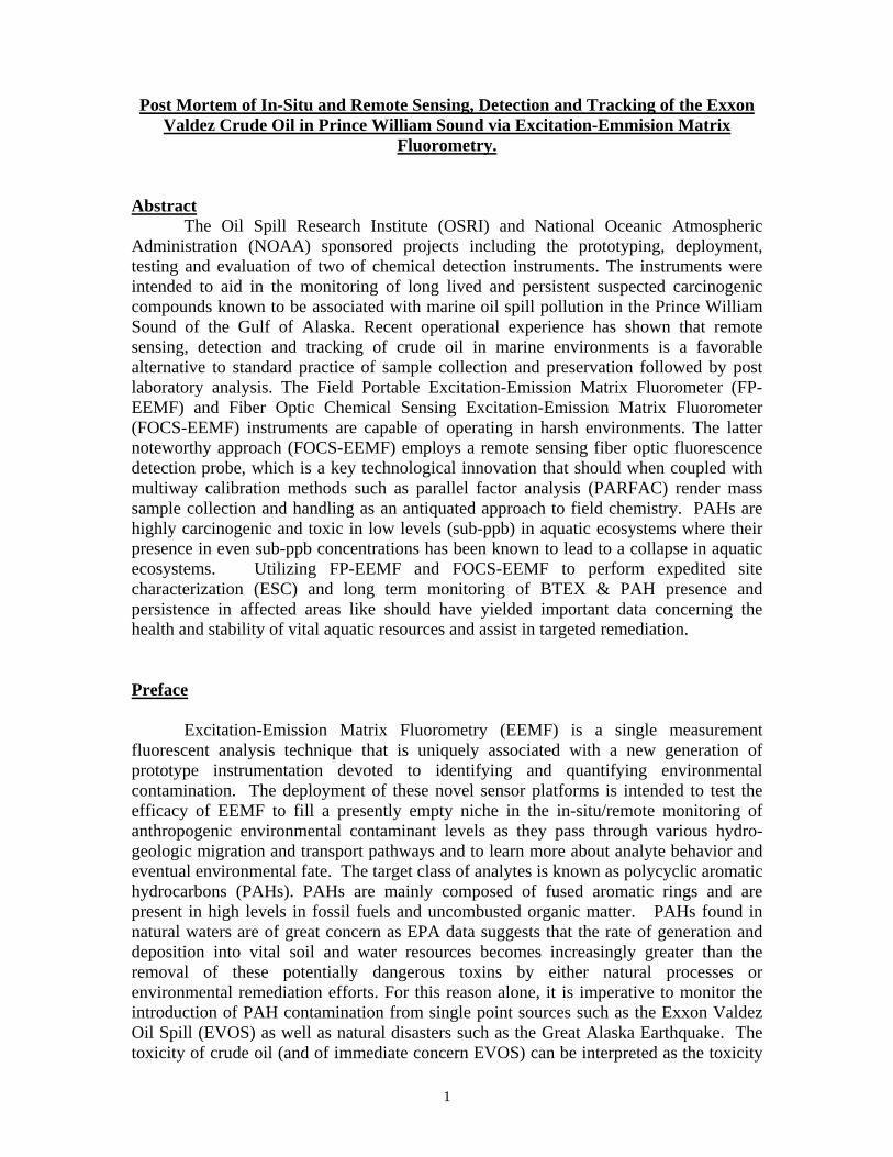
Fluorescence is one of the two luminescence methods used in spectroscopy. The other method is phosphorescence. The difference between these two methods can easiest be explained if we go down to the electronic level of the molecule. A paired electron in the ground state has two possible excitation levels (see

Figure 1). One is where the excited electron is paired to the second electron in the ground state, and thus the return to the ground state is spin-allowed and occurs rapidly (typically in 10-8s). The other option is that the excited electron has the same spin as the electron in the ground state. In this configuration the transition to the ground state is forbidden, and it thus occurs slowly (typically in the range of 1ms-1s).

Figure 1: The ground state, and the two possible excitation states. The only one giving fluorescence is the

excited single state.

4

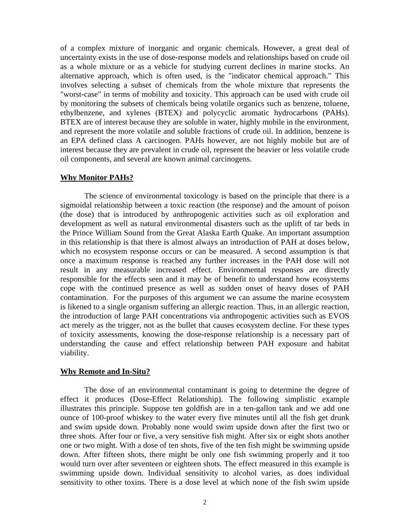
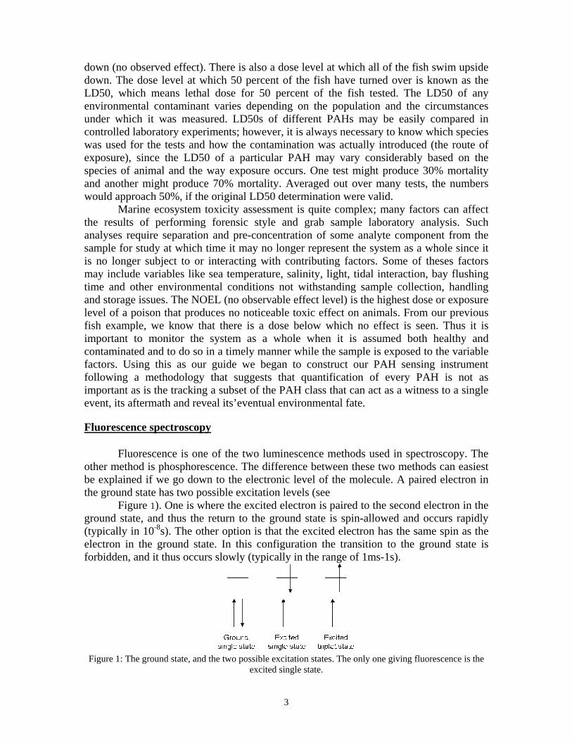
The Excitation-Emission Matrix A common way of measuring fluorescence spectrum is to excite a sample at a certain wavelength, and the emitted light can be detected in a range of wavelengths. It is also possible to excite the sample at different wavelengths, and then only measure the emission at one single wavelength. This way of measurement makes it easier to visually inspect a group of samples, but by doing so all the available information is not recorded. Another way of collecting data from a fluorescence instrument is to collect several emission spectra at different excitation wavelengths. From this procedure the emission spectra can be set side-by-side thus creating a fluorescence landscape, with the excitation wavelength along the y-axis, the emission along the y-axis and the intensity of the signal along the x-axis and fluorescence intensity along the z-axis. This landscape is also known as the excitation-emission-matrix, shortened EEM.

Emission λ

Exci

tatio

n λ

Sample

Emission λ

Exci

tatio

n λ

Sample

Emission λ

Exci

tatio

n λ

Sample

Emission λ

Exci

tatio

n λ

Sample

Emission λ

Exci

tatio

n λ

Sample

Emission λ

Exci

tatio

n λ

Sample

Emission λ

Exci

tatio

n λ

Sample

Emission λ

Exci

tatio

n λ

Sample

Emission λ

Exci

tatio

n λ

Sample

Emission λ

Exci

tatio

n λ

Sample

Emission λ

Exci

tatio

n λ

Sample

Emission λ

Exci

tatio

n λ

Sample

Emission λ

Exci

tatio

n λ

Sample

Emission λ

Exci

tatio

n λ

Sample

Fig 2.0 excitation (y) emission(x) axis Fig 2.1 view looking down the intensity (z) axis

Benefits of the EEM include: Detection Limits. The EEMF has detection limits for polycyclic aromatic hydrocarbons (PAHs) in natural water lower than the PQL of GC-MS following extraction and pre-concentration. Many environmental contaminants have detection limits lower than EPA action limits for groundwater. Speed. An entire EEMF analyses is completed in 2 minutes. This compares to 30 minutes for GC-MS (not counting the extraction and pre-concentration time). Collection of an EEMF landscape with a scanning fluorometer would require 30 minutes with the same spectral resolution and S/N. In-Situ Monitoring. With the battery power and fiber optic probe, the EEMF is ideally constructed for field screening of ‘interesting’ samples and monitoring the migration of a pollution plume. Multi-Analyte Analyses. Because a wide spectral range, EEMF landscapes collected for each sample can be used in conjunction with advanced multi-way chemometric methods to accurately resolve the spectral signatures of many classes of analytes simultaneously.

Emission (nm)

Exci

tatio

n (n

m)

EEM

Emission (nm)

Exci

tatio

n (n

m)

Emission (nm)

Exci

tatio

n (n

m)

EEM

5

Part One: Operational Concept of Field Portable Excitation-Emission Matrix Fluorometer (FP-EEMF)

The objective of this initial project was to develop and optimize a prototype single

measurement, Excitation-Emission Matrix (EEM) fluorescence instrument for target applications in environmental screening for organic pollutants,(i.e. BTEX and PAHs) This platform combines EEM fluorescence spectroscopy and advanced multi-way calibration models to enable current field instruments that are:

• Inexpensive and field portable • Provide on-site, real time analysis • Minimalize reagent use and sample pretreatment • Capable of sub-ppb aqueous PAH detection • Have low detection limits • Greatly reduce data collection and analysis time: • Have good spectral resolution • Requires no field standards

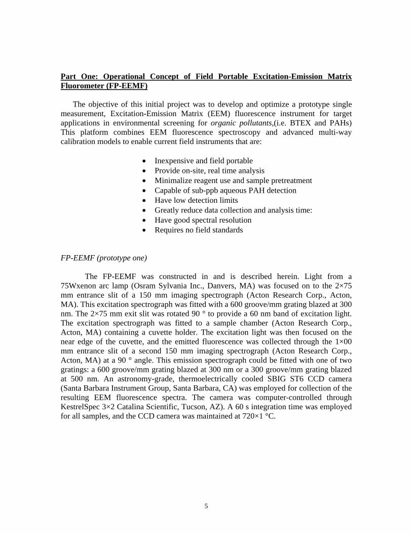
FP-EEMF (prototype one)

The FP-EEMF was constructed in and is described herein. Light from a 75Wxenon arc lamp (Osram Sylvania Inc., Danvers, MA) was focused on to the 2×75 mm entrance slit of a 150 mm imaging spectrograph (Acton Research Corp., Acton, MA). This excitation spectrograph was fitted with a 600 groove/mm grating blazed at 300 nm. The 2×75 mm exit slit was rotated 90 ° to provide a 60 nm band of excitation light. The excitation spectrograph was fitted to a sample chamber (Acton Research Corp., Acton, MA) containing a cuvette holder. The excitation light was then focused on the near edge of the cuvette, and the emitted fluorescence was collected through the 1×00 mm entrance slit of a second 150 mm imaging spectrograph (Acton Research Corp., Acton, MA) at a 90 ° angle. This emission spectrograph could be fitted with one of two gratings: a 600 groove/mm grating blazed at 300 nm or a 300 groove/mm grating blazed at 500 nm. An astronomy-grade, thermoelectrically cooled SBIG ST6 CCD camera (Santa Barbara Instrument Group, Santa Barbara, CA) was employed for collection of the resulting EEM fluorescence spectra. The camera was computer-controlled through KestrelSpec 3×2 Catalina Scientific, Tucson, AZ). A 60 s integration time was employed for all samples, and the CCD camera was maintained at 720×1 °C.

6

150mm F/4Imaging

Spectrograph

Sample

75 WattXenon ArcLampCCD

Camera 300 g/mm grating

600 g/mm grating150mm F/4Imaging

Spectrograph150mm F/4

ImagingSpectrograph

Sample




Spectrograph150mm F/4

ImagingSpectrograph

Sample




Spectrograph

excitation spectrograph

emission spectrograph

Lamp

CCD

sample chamber

12 V 75 A Deep Cycle batteries

AC Ignition Transformer*

* DC Transformer not shown

excitation spectrograph

emission spectrograph

Lamp

CCD

sample chamber

12 V 75 A Deep Cycle batteries

AC Ignition Transformer*

* DC Transformer not shown

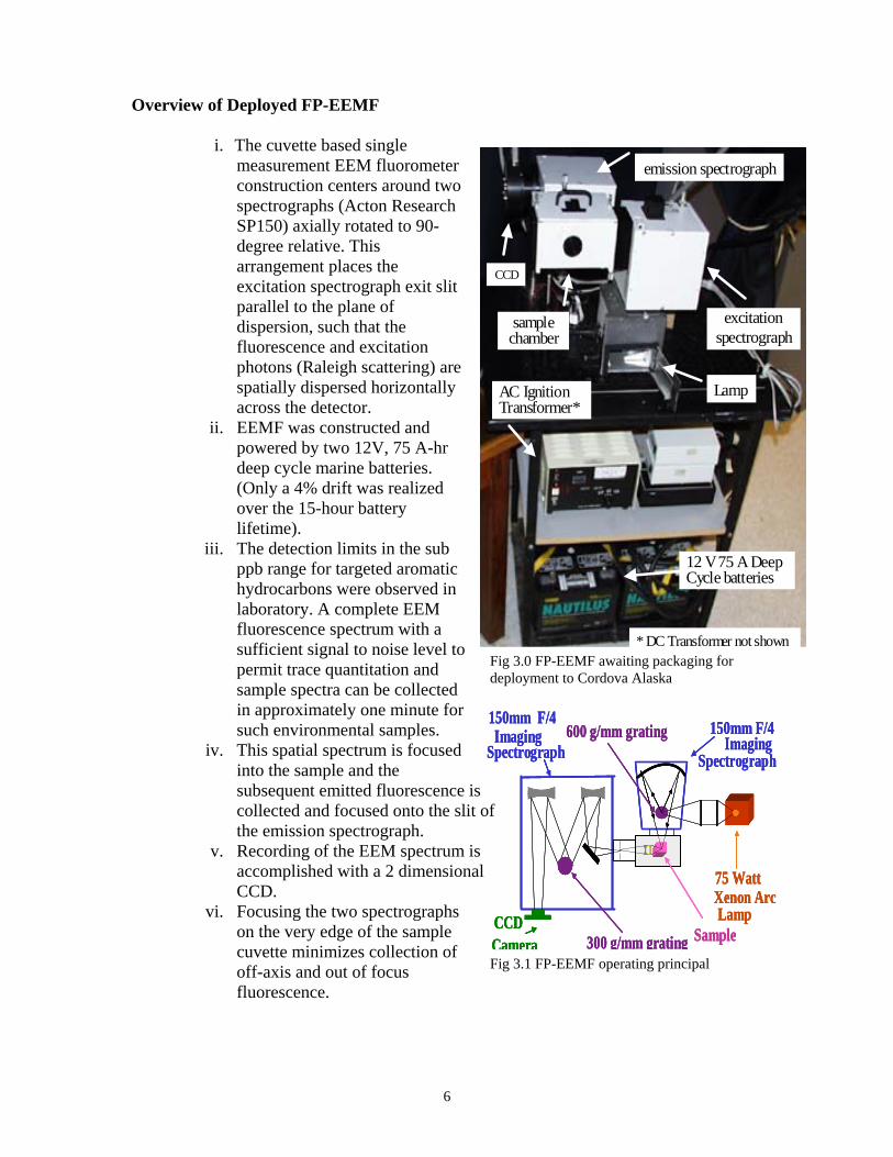
Overview of Deployed FP-EEMF

i. The cuvette based single measurement EEM fluorometer construction centers around two spectrographs (Acton Research SP150) axially rotated to 90-degree relative. This arrangement places the excitation spectrograph exit slit parallel to the plane of dispersion, such that the fluorescence and excitation photons (Raleigh scattering) are spatially dispersed horizontally across the detector.

ii. EEMF was constructed and powered by two 12V, 75 A-hr deep cycle marine batteries. (Only a 4% drift was realized over the 15-hour battery lifetime).

iii. The detection limits in the sub ppb range for targeted aromatic hydrocarbons were observed in laboratory. A complete EEM fluorescence spectrum with a sufficient signal to noise level to permit trace quantitation and sample spectra can be collected in approximately one minute for such environmental samples.

iv. This spatial spectrum is focused into the sample and the subsequent emitted fluorescence is collected and focused onto the slit of the emission spectrograph.

v. Recording of the EEM spectrum is accomplished with a 2 dimensional CCD.

vi. Focusing the two spectrographs on the very edge of the sample cuvette minimizes collection of off-axis and out of focus fluorescence.

Fig 3.0 FP-EEMF awaiting packaging for deployment to Cordova Alaska

Fig 3.1 FP-EEMF operating principal

7

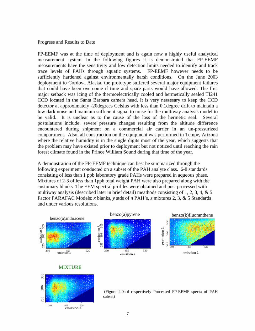
Progress and Results to Date FP-EEMF was at the time of deployment and is again now a highly useful analytical measurement system. In the following figures it is demonstrated that FP-EEMF measurements have the sensitivity and low detection limits needed to identify and track trace levels of PAHs through aquatic systems. FP-EEMF however needs to be sufficiently hardened against environmentally harsh conditions. On the June 2003 deployment to Cordova Alaska, the prototype suffered several major equipment failures that could have been overcome if time and spare parts would have allowed. The first major setback was icing of the thermoelectrically cooled and hermetically sealed TI241 CCD located in the Santa Barbara camera head. It is very nessesary to keep the CCD detector at approximately -20degrees Celsius with less than 0.1degree drift to maintain a low dark noise and maintain sufficient signal to noise for the multiway analysis model to be valid. It is unclear as to the cause of the loss of the hermetic seal. Several postulations include; severe pressure changes resulting from the altitude difference encountered during shipment on a commercial air carrier in an un-pressurized compartment. Also, all construction on the equipment was performed in Tempe, Arizona where the relative humidity is in the single digits most of the year, which suggests that the problem may have existed prior to deployment but not noticed until reaching the rain forest climate found in the Prince William Sound during that time of the year. A demonstration of the FP-EEMF technique can best be summarized through the following experiment conducted on a subset of the PAH analyte class. 6-8 standards consisting of less than 1 ppb laboratory grade PAHs were prepared in aqueous phase. Mixtures of 2-3 of less than 1ppb total weight PAH were also prepared along with the customary blanks. The EEM spectral profiles were obtained and post processed with multiway analysis (described later in brief detail) meathods consisting of 1, 2, 3, 4, & 5 Factor PARAFAC Models: x blanks, y stds of n PAH’s, z mixtures 2, 3, & 5 Standards and under various resolutions.

(Figure 4.0a-d respectively Processed FP-EEMF specta of PAH subset)

benzo(k)fluoranthene

255

286

305

exci

tatio

n λ

emission λ

390 455 520 255

286

305

390 455 520

exci

tatio

n λ

emission λ

benzo(a)anthracene

255

286

305

390 455 520

exci

tatio

n λ

emission λ

benzo(a)pyrene

MIXTURE

255

286

305

emission λ 390 455 520

8

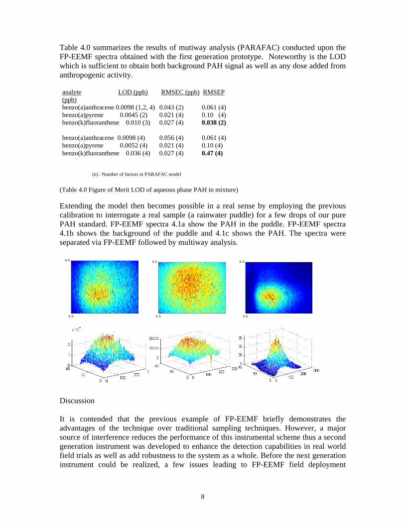
Table 4.0 summarizes the results of mutiway analysis (PARAFAC) conducted upon the FP-EEMF spectra obtained with the first generation prototype. Noteworthy is the LOD which is sufficient to obtain both background PAH signal as well as any dose added from anthropogenic activity.

(Table 4.0 Figure of Merit LOD of aqueous phase PAH in mixture) Extending the model then becomes possible in a real sense by employing the previous calibration to interrogate a real sample (a rainwater puddle) for a few drops of our pure PAH standard. FP-EEMF spectra 4.1a show the PAH in the puddle. FP-EEMF spectra 4.1b shows the background of the puddle and 4.1c shows the PAH. The spectra were separated via FP-EEMF followed by multiway analysis.

Discussion It is contended that the previous example of FP-EEMF briefly demonstrates the advantages of the technique over traditional sampling techniques. However, a major source of interference reduces the performance of this instrumental scheme thus a second generation instrument was developed to enhance the detection capabilities in real world field trials as well as add robustness to the system as a whole. Before the next generation instrument could be realized, a few issues leading to FP-EEMF field deployment

0.5

0.5

0.5

0.5

0.5

0.5

analyte LOD (ppb) RMSEC (ppb) RMSEP (ppb) benzo(a)anthracene 0.0098 (1,2, 4) 0.043 (2) 0.061 (4) benzo(a)pyrene 0.0045 (2) 0.021 (4) 0.10 (4) benzo(k)fluoranthene 0.010 (3) 0.027 (4) 0.038 (2) benzo(a)anthracene 0.0098 (4) 0.056 (4) 0.061 (4) benzo(a)pyrene 0.0052 (4) 0.021 (4) 0.10 (4) benzo(k)fluoranthene 0.036 (4) 0.027 (4) 0.47 (4)

(n) : Number of factors in PARAFAC model

9

limitations had to be recognized and dealt with. The leading issue is discussed in the next section.

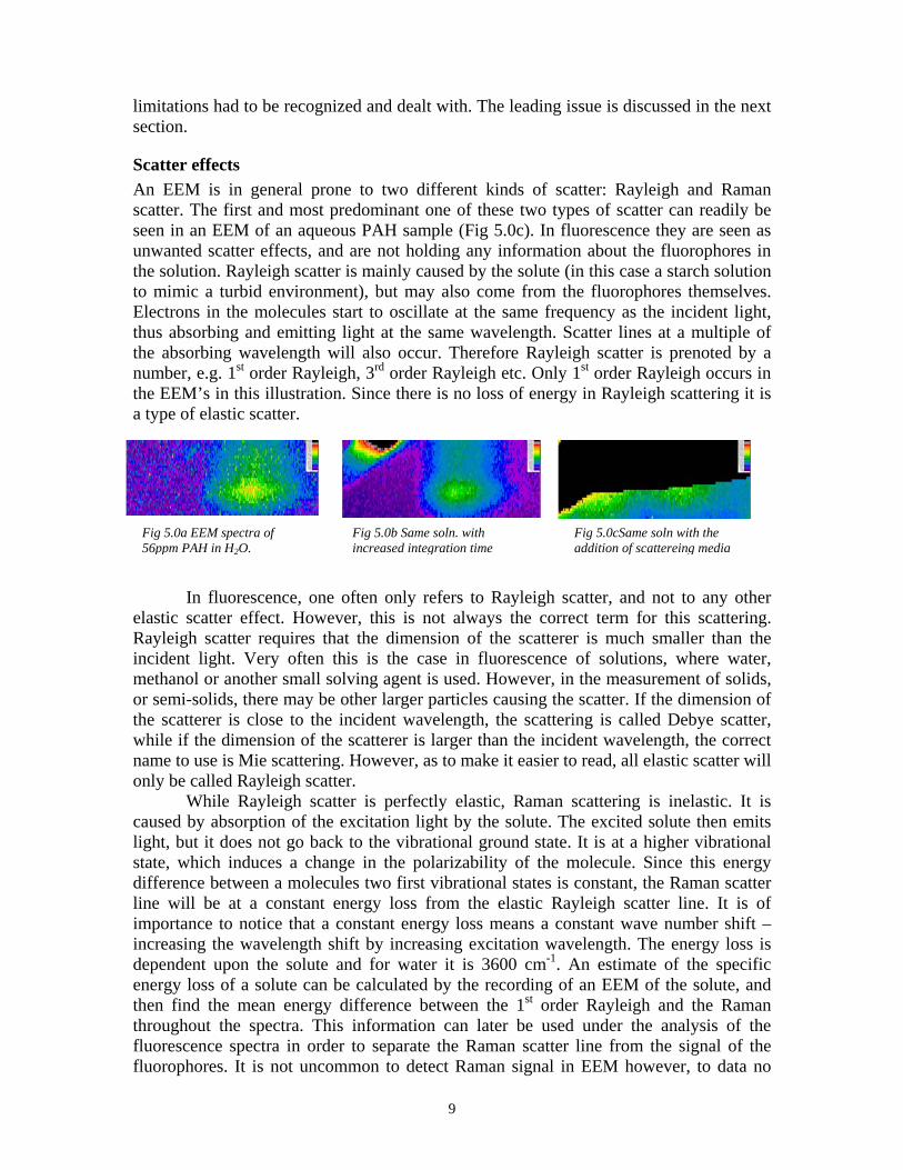
Scatter effects An EEM is in general prone to two different kinds of scatter: Rayleigh and Raman scatter. The first and most predominant one of these two types of scatter can readily be seen in an EEM of an aqueous PAH sample (Fig 5.0c). In fluorescence they are seen as unwanted scatter effects, and are not holding any information about the fluorophores in the solution. Rayleigh scatter is mainly caused by the solute (in this case a starch solution to mimic a turbid environment), but may also come from the fluorophores themselves. Electrons in the molecules start to oscillate at the same frequency as the incident light, thus absorbing and emitting light at the same wavelength. Scatter lines at a multiple of the absorbing wavelength will also occur. Therefore Rayleigh scatter is prenoted by a number, e.g. 1st order Rayleigh, 3rd order Rayleigh etc. Only 1st order Rayleigh occurs in the EEM’s in this illustration. Since there is no loss of energy in Rayleigh scattering it is a type of elastic scatter.

In fluorescence, one often only refers to Rayleigh scatter, and not to any other elastic scatter effect. However, this is not always the correct term for this scattering. Rayleigh scatter requires that the dimension of the scatterer is much smaller than the incident light. Very often this is the case in fluorescence of solutions, where water, methanol or another small solving agent is used. However, in the measurement of solids, or semi-solids, there may be other larger particles causing the scatter. If the dimension of the scatterer is close to the incident wavelength, the scattering is called Debye scatter, while if the dimension of the scatterer is larger than the incident wavelength, the correct name to use is Mie scattering. However, as to make it easier to read, all elastic scatter will only be called Rayleigh scatter.

While Rayleigh scatter is perfectly elastic, Raman scattering is inelastic. It is caused by absorption of the excitation light by the solute. The excited solute then emits light, but it does not go back to the vibrational ground state. It is at a higher vibrational state, which induces a change in the polarizability of the molecule. Since this energy difference between a molecules two first vibrational states is constant, the Raman scatter line will be at a constant energy loss from the elastic Rayleigh scatter line. It is of importance to notice that a constant energy loss means a constant wave number shift – increasing the wavelength shift by increasing excitation wavelength. The energy loss is dependent upon the solute and for water it is 3600 cm-1. An estimate of the specific energy loss of a solute can be calculated by the recording of an EEM of the solute, and then find the mean energy difference between the 1st order Rayleigh and the Raman throughout the spectra. This information can later be used under the analysis of the fluorescence spectra in order to separate the Raman scatter line from the signal of the fluorophores. It is not uncommon to detect Raman signal in EEM however, to data no

Fig 5.0a EEM spectra of 56ppm PAH in H2O.

Fig 5.0b Same soln. with increased integration time

Fig 5.0cSame soln with the addition of scattereing media

10

great effort has made in the course of this investigation to make use of it in an analytical sense.

Fig 5.0c also is illustrative of the next most pressing issue in the persuit of remote and in-situ analysis of environmental contamination. CCD detectors are prone to blooming. Blooming is a saturation of adjacent pixels due to the overfilling of the saturation potential (Vsat ) of the active photosite. This problem is especially apparent when conducting analysis of PAH samples in turbid environment where a long integration may cause Rayleigh scattering to overrun a fluorophore signal prior to gaining enough signal for processing. The spectral information contained in the bloomed pixels is presumed lost. Anti-blooming gates which can be both physical and virtual can be employed with the TI241 detector but come at a cost of increased background noise and an overall reduction of the dynamic range of the detector purported by the manufactutrer to be ~72dB. In the following section containing generation 2 of the EEMF series of prototypes that was also deployed to Cordova Alaska in 2003, this issue is dealt with successfully.

Part Two Operational Concept of Remote Sensing Fiber-Optic Excitation-Emission Matrix Fluorometer

A second smaller prototype EEMF has been constructed with a fiber optic probe.

This system weighs only 30 lbs. And has an 8 hour functional lifetime on a single 12V 35 amp-hour battery. The single measurement fiber optic excitation-emission matrix fluorometer (FOCS-EEMF) has developed for rapid field screening of potentially contaminated natural waters. The sensor system employs a fiber optic probe for direct in situ analysis of liquid and solid surfaces. The FOCS-EEMF uses a 75W zenon arc lap and a Kodak 1602E 2-dimensional CCD mounted in an in house manufactured camera head for detection. The FOCS-EEMF can access excitation wavelengths as low as 220 nm and emission wavelengths as high as 950 nm. This version is designed for screening of naturally fluorescent components in fuels and petroleum products as well as other fluorescent contaminants . Combined with multi-way spectral resolution and calibration methods, the structure of the FOCS-EEMF landscapes can be exploited to extract the signature of many compounds from the native fluorescent background.

Fig 6.0a FOCS-EEMF probe under illuminated conditions.

Fig 6.0b FOCS-EEMF in unhardended, unshielded configuration during laboratory testing.

11

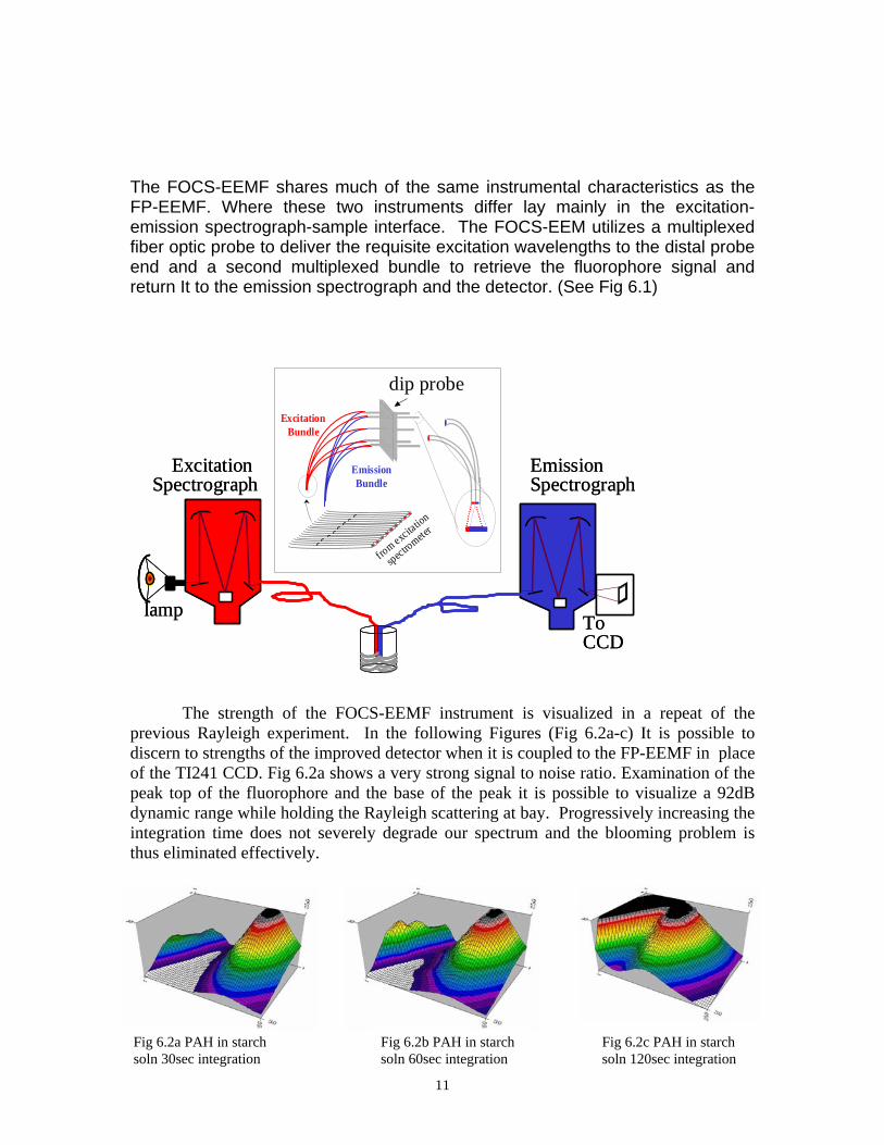
The FOCS-EEMF shares much of the same instrumental characteristics as the FP-EEMF. Where these two instruments differ lay mainly in the excitation-emission spectrograph-sample interface. The FOCS-EEM utilizes a multiplexed fiber optic probe to deliver the requisite excitation wavelengths to the distal probe end and a second multiplexed bundle to retrieve the fluorophore signal and return It to the emission spectrograph and the detector. (See Fig 6.1)

The strength of the FOCS-EEMF instrument is visualized in a repeat of the

previous Rayleigh experiment. In the following Figures (Fig 6.2a-c) It is possible to discern to strengths of the improved detector when it is coupled to the FP-EEMF in place of the TI241 CCD. Fig 6.2a shows a very strong signal to noise ratio. Examination of the peak top of the fluorophore and the base of the peak it is possible to visualize a 92dB dynamic range while holding the Rayleigh scattering at bay. Progressively increasing the integration time does not severely degrade our spectrum and the blooming problem is thus eliminated effectively.

ExcitationBundle

EmissionBundle

from excitation

spectrometer

lamp

Emission Spectrograph

To CCD

Excitation Spectrograph

lamp

Emission Spectrograph

To CCD

Excitation Spectrograph

dip probe

Fig 6.2a PAH in starch soln 30sec integration

Fig 6.2c PAH in starch soln 120sec integration

Fig 6.2b PAH in starch soln 60sec integration

12

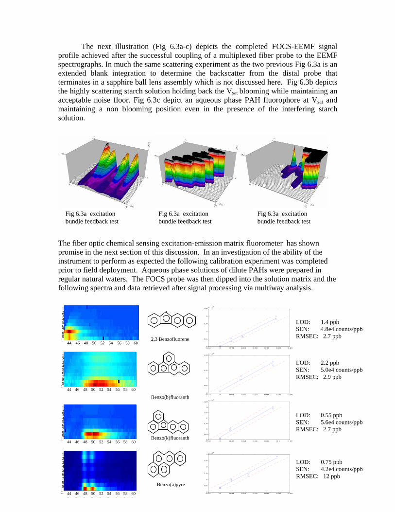
The next illustration (Fig 6.3a-c) depicts the completed FOCS-EEMF signal profile achieved after the successful coupling of a multiplexed fiber probe to the EEMF spectrographs. In much the same scattering experiment as the two previous Fig 6.3a is an extended blank integration to determine the backscatter from the distal probe that terminates in a sapphire ball lens assembly which is not discussed here. Fig 6.3b depicts the highly scattering starch solution holding back the Vsat blooming while maintaining an acceptable noise floor. Fig 6.3c depict an aqueous phase PAH fluorophore at Vsat and maintaining a non blooming position even in the presence of the interfering starch solution.

The fiber optic chemical sensing excitation-emission matrix fluorometer has shown promise in the next section of this discussion. In an investigation of the ability of the instrument to perform as expected the following calibration experiment was completed prior to field deployment. Aqueous phase solutions of dilute PAHs were prepared in regular natural waters. The FOCS probe was then dipped into the solution matrix and the following spectra and data retrieved after signal processing via multiway analysis.

-0.01 0 0.01 0.02 0.03 0.04 0.05 0.060

0.5

1

1.5

2

2.5x 106

LOD: 2.2 ppb SEN: 5.0e4 counts/ppb RMSEC: 2.9 ppb

-0.02 0 0.02 0.04 0.06 0.08 0.1 0.120

0.5

1

1.5

2

2.5

3

3.5x 106


-0.01 0 0.01 0.02 0.03 0.04 0.05 0.060

0.5

1

1.5

2

2.5x 106


-0.01 0 0.01 0.02 0.03 0.04 0.05 0.060

0.5

1

1.5

2

2.5

3x 106

LOD: 0.75 ppb SEN: 4.2e4 counts/ppb RMSEC: 12 ppb

44 46 48 50 52 54 56 58 60

123456789

1 2,3 Benzofluorene

44 46 48 50 52 54 56 58 60

123456789

1

Benzo(b)fluoranth

44 46 48 50 52 54 56 58 60

123456789

1 Benzo(k)fluoranth

440

460

480

500

520

540

560

580

600

123456789

10

Benzo(a)pyre

Fig 6.3a excitation bundle feedback test



13

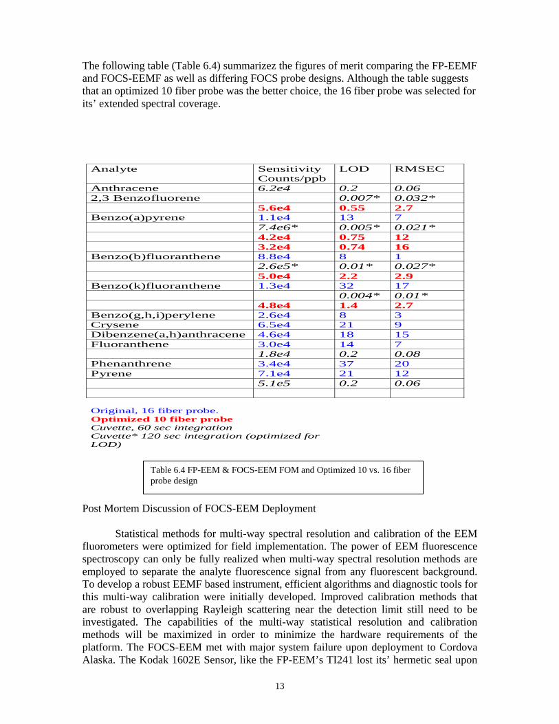
The following table (Table 6.4) summarizez the figures of merit comparing the FP-EEMF and FOCS-EEMF as well as differing FOCS probe designs. Although the table suggests that an optimized 10 fiber probe was the better choice, the 16 fiber probe was selected for its’ extended spectral coverage.

Post Mortem Discussion of FOCS-EEM Deployment

Statistical methods for multi-way spectral resolution and calibration of the EEM fluorometers were optimized for field implementation. The power of EEM fluorescence spectroscopy can only be fully realized when multi-way spectral resolution methods are employed to separate the analyte fluorescence signal from any fluorescent background. To develop a robust EEMF based instrument, efficient algorithms and diagnostic tools for this multi-way calibration were initially developed. Improved calibration methods that are robust to overlapping Rayleigh scattering near the detection limit still need to be investigated. The capabilities of the multi-way statistical resolution and calibration methods will be maximized in order to minimize the hardware requirements of the platform. The FOCS-EEM met with major system failure upon deployment to Cordova Alaska. The Kodak 1602E Sensor, like the FP-EEM’s TI241 lost its’ hermetic seal upon

Analyte Sensitivity Counts/ppb

LOD RMSEC

Anthracene 6.2e4 0.2 0.06 2,3 Benzofluorene 0.007* 0.032* 5.6e4 0.55 2.7 Benzo(a)pyrene 1.1e4 13 7 7.4e6* 0.005* 0.021* 4.2e4 0.75 12 3.2e4 0.74 16 Benzo(b)fluoranthene 8.8e4 8 1 2.6e5* 0.01* 0.027* 5.0e4 2.2 2.9 Benzo(k)fluoranthene 1.3e4 32 17 0.004* 0.01* 4.8e4 1.4 2.7 Benzo(g,h,i)perylene 2.6e4 8 3 Crysene 6.5e4 21 9 Dibenzene(a,h)anthracene 4.6e4 18 15 Fluoranthene 3.0e4 14 7 1.8e4 0.2 0.08 Phenanthrene 3.4e4 37 20 Pyrene 7.1e4 21 12 5.1e5 0.2 0.06 Original, 16 fiber probe. Optimized 10 fiber probe Cuvette, 60 sec integration Cuvette* 120 sec integration (optimized for LOD)

Table 6.4 FP-EEM & FOCS-EEM FOM and Optimized 10 vs. 16 fiber probe design

14

initial cooling iced over and was renderered permanently disabled. Other problems were also evident after a commercial flight indicating that such sensors need to re-sealed after arriving in the field and before operation. A new generation of FOCS-EEM is currently under construction which addresses this issue as well as some practical issues surrounding weight and portability as well as longevity on station. It is expected that the new generation will be acceptable to commercial carriers as a “carry-on” thus the filed team can monitor and ensure safe transport to the investigation site. \ Mutiway Analysis and Chemometrics

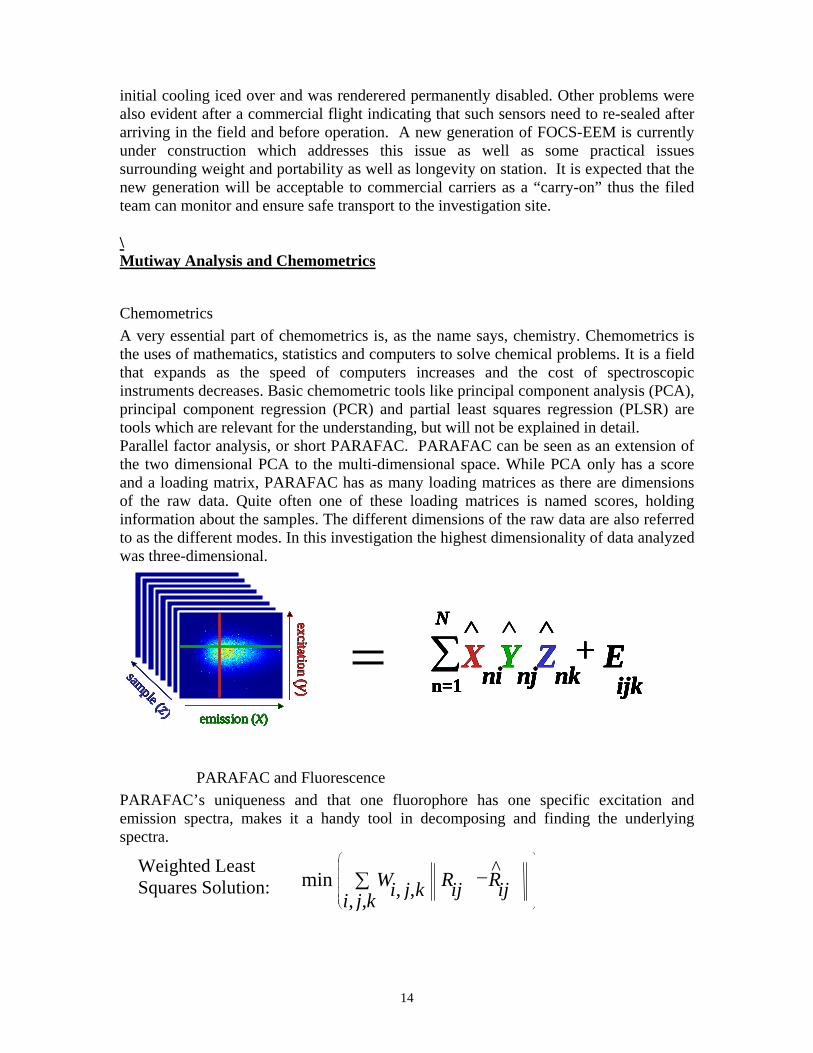
Chemometrics A very essential part of chemometrics is, as the name says, chemistry. Chemometrics is the uses of mathematics, statistics and computers to solve chemical problems. It is a field that expands as the speed of computers increases and the cost of spectroscopic instruments decreases. Basic chemometric tools like principal component analysis (PCA), principal component regression (PCR) and partial least squares regression (PLSR) are tools which are relevant for the understanding, but will not be explained in detail. Parallel factor analysis, or short PARAFAC. PARAFAC can be seen as an extension of the two dimensional PCA to the multi-dimensional space. While PCA only has a score and a loading matrix, PARAFAC has as many loading matrices as there are dimensions of the raw data. Quite often one of these loading matrices is named scores, holding information about the samples. The different dimensions of the raw data are also referred to as the different modes. In this investigation the highest dimensionality of data analyzed was three-dimensional.

PARAFAC and Fluorescence PARAFAC’s uniqueness and that one fluorophore has one specific excitation and emission spectra, makes it a handy tool in decomposing and finding the underlying spectra.

sample (z) emission (x)

excitation (y )


excitation (y)


excitation ( y)


excitation (y )


excitation (y)


excitation ( y)


excitation (y )


excitation (y )


excitation (y)


excitation ( y)

Weighted Least Squares Solution: min , ,

^

, ,

W i j k R ij R iji j k

− ∑

⎛

⎝

⎜ ⎜ ⎜ ⎜ ⎜

⎞

⎠

=ijknknjni

N

EZYX +∧

∑n=1

∧ ∧

ijknknjni

N

EZYX +∧

∑n=1

∧

ijknknjni

N

EZYX +∧

∑n=1

∧ ∧

ijknknjni

N

EZYX +∧

∑n=1

∧

ijknknjni

N

EZYX +∧

∑n=1

∧ ∧

ijknknjni

N

EZYX +∧

∑n=1

∧

15

Documents

Post Mortem of In-Situ and Remote Sensing, Detection and