Submitted to BernoulliarXiv: 1406.4406v1

Posterior concentration rates for empirical

Bayes procedures with applications to

Dirichlet process mixturesSOPHIE DONNET1 VINCENT RIVOIRARD2 JUDITH ROUSSEAU3 and CATIASCRICCIOLO4

1UMR MIA-Paris, AgroParisTech, INRA, Universite Paris-Saclay, 75005, Paris, France.E-mail: sophie.donnet@agroparistech.fr

2CEREMADE, Universite Paris-Dauphine, Place du Marechal de Lattre de Tassigny, 75775Paris Cedex 16, France. E-mail: rivoirard@ceremade.dauphine.fr

3CEREMADE, Universite Paris-Dauphine, Place du Marechal de Lattre de Tassigny, 75775Paris Cedex 16, FranceandCREST-ENSAE, 3 Avenue Pierre Larousse, 92240 Malakoff, France.E-mail: rousseau@ceremade.dauphine.fr

4Department of Economics, University of Verona, Via Cantarane 24, 37129 Verona, Italy.E-mail: catia.scricciolo@univr.it

We provide conditions on the statistical model and the prior probability law to derive con-traction rates of posterior distributions corresponding to data-dependent priors in an empiricalBayes approach for selecting prior hyper-parameter values. We aim at giving conditions in thesame spirit as those in the seminal article of Ghosal and van der Vaart [23]. We then applythe result to specific statistical settings: density estimation using Dirichlet process mixtures ofGaussian densities with base measure depending on data-driven chosen hyper-parameter valuesand intensity function estimation of counting processes obeying the Aalen model. In the formersetting, we also derive recovery rates for the related inverse problem of density deconvolution.In the latter, a simulation study for inhomogeneous Poisson processes illustrates the results.

Keywords: Aalen model, counting processes, Dirichlet process mixtures, empirical Bayes, poste-rior contraction rates.

1. Introduction

In a Bayesian approach to statistical inference, the prior distribution should, in principle,be chosen independently of the data; however, it is not always an easy task to elicit theprior hyper-parameter values and a common practice is to replace them by summariesof the data. The prior is then data-dependent and the approach falls under the umbrellaof empirical Bayes methods, as opposed to fully Bayes methods. Consider a statistical

1

2 S. Donnet et al.

model (P(n)θ : θ ∈ Θ) on a sample space X (n), together with a family of prior distributions

(π(· | γ) : γ ∈ Γ) on a parameter space Θ. A Bayesian statistician would either setthe hyper-parameter γ to a specific value γ0 or integrate it out using a probabilitydistribution for it in a hierarchical specification of the prior for θ. Both approacheswould lead to prior distributions for θ that do not depend on the data. However, it isoften the case that knowledge is not a priori available to either fix a value for γ or elicita prior distribution for it, so that a value for γ can be more easily chosen using thedata. Throughout the paper, we will denote by γn a data-driven choice for γ. There aremany instances in the literature where an empirical Bayes choice for the prior hyper-parameters is performed, sometimes without explicitly mentioning it. Some examplesconcerning the parametric case can be found in Ahmed and Reid [2], Berger [6] andCasella [8]. Regarding the nonparametric case, Richardson and Green [36] propose adefault empirical Bayes approach to deal with parametric and nonparametric mixturesof Gaussian densities; McAuliffe et al. [33] propose another empirical Bayes approach forDirichlet process mixtures of Gaussian densities, while in Szabo et al. [50] an empiricalBayes procedure is proposed in the context of the Gaussian white noise model to obtainrate adaptive posterior distributions. There are many other instances of empirical Bayesmethods in the literature, especially in applied problems.

Our aim is not to claim that empirical Bayes methods are somehow better than fullyBayes methods, rather to provide tools to study frequentist asymptotic properties ofempirical Bayes posterior distributions, given their wide use in practice. Very little isknown about the asymptotic behavior of such empirical Bayes posterior distributionsin a general framework. It is a common belief that if γn asymptotically converges tosome value γ∗, then the empirical Bayes posterior distribution associated with γn iseventually “close” to the fully Bayes posterior associated with γ∗. Results have beenobtained in specific statistical settings by Clyde and George [10], Cui and George [11] forwavelets or variable selection, by Szabo et al. [48, 49, 50] for the Gaussian white noisemodel, by Scricciolo [43] for conditional density estimation, by Sniekers and van der Vaart[47], Serra and Krivobokova [44] for Gaussian regression with Gaussian priors. Recently,Petrone et al. [34] have investigated asymptotic properties of empirical Bayes posteriordistributions obtaining general conditions for consistency and, in the parametric case, forstrong merging between fully Bayes and maximum marginal likelihood empirical Bayesposterior distributions.

In this article, we are interested in studying the frequentist asymptotic behaviour ofempirical Bayes posterior distributions in terms of contraction rates. Let d(·, ·) be a lossfunction on Θ, say a pseudo-metric. For θ0 ∈ Θ and ε > 0, let Uε := θ : d(θ, θ0) ≤ ε bea neighborhood of θ0. The empirical Bayes posterior distribution is said to concentrateat θ0 with rate εn relative to d, where εn is a positive sequence converging to zero, if the

empirical Bayes posterior probability of the set Uεn tends to one in P(n)θ0

-probability. Inthe case of fully Bayes procedures, there has been so far a vast literature on posteriorconsistency and contraction rates since the seminal articles of Barron et al. [4] and Ghosalet al. [22]. Following ideas of Schwartz [41], Ghosal et al. [22] in the case of independentand identically distributed (iid) observations and Ghosal and van der Vaart [23] in the

Empirical Bayes posterior concentration rates 3

case of non-iid observations have developed an elegant and powerful methodology toassess posterior contraction rates which boils down to lower bounding the prior mass of

Kullback-Leibler type neighborhoods of P(n)θ0

and to constructing exponentially powerfultests for testing H0 : θ = θ0 against H1 : θ ∈ θ′ : d(θ′, θ0) > εn. However, thisapproach cannot be immediately taken to deal with posterior distributions correspondingto data-dependent priors. In this article, we develop a similar methodology for assessingposterior contraction rates in the case where the prior distribution depends on the datathrough a data-driven choice γn for γ.

In Theorem 1, we provide sufficient conditions for deriving contraction rates of em-pirical Bayes posterior distributions, in the same spirit as those presented in Theorem 1of Ghosal and van der Vaart [23]. To our knowledge, this is the first result on posteriorcontraction rates for data-dependent priors which is neither model nor prior specific. Thetheorem is then applied to nonparametric mixture models. Two relevant applications areconsidered: Dirichlet process mixtures of Gaussian densities for the problems of densityestimation and density deconvolution in Section 3; Dirichlet process mixtures of uniformdensities for estimating intensity functions of counting processes obeying the Aalen modelin Section 4. Theorem 1 has also been applied to Gaussian process priors and sieve priorsin Rousseau and Szabo [38].

Dirichlet process mixtures (DPM) have been introduced by Ferguson [20] and haveproved to be a major tool in Bayesian nonparametrics, see for instance Hjort et al. [28].Rates of convergence for fully Bayes posterior distributions corresponding to DPM ofGaussian densities have been widely studied: they lead to minimax-optimal, possibly upto a logarithmic factor, estimation procedures over a wide collection of density functionclasses, see Ghosal and van der Vaart [24, 25], Kruijer et al. [31], Scricciolo [42] andShen et al. [45]. In Section 3.1, we extend existing results to the case of a Gaussian basemeasure for the Dirichlet process prior with data-driven chosen mean and variance, asadvocated for instance in Richardson and Green [36]. Furthermore, in Section 3.2, dueto some new inversion inequalities, we get, as a by-product, empirical Bayes posteriorrecovery rates for the problem of density deconvolution when the error distribution iseither ordinary or super-smooth and the mixing density is modeled as a DPM of normaldensities with a Gaussian base measure having data-driven selected mean and variance.The problem of Bayesian density deconvolution when the mixing density is modeled as aDPM of Gaussian densities and the error distribution is super-smooth has been recentlystudied by Sarkar et al. [40].

In Section 4, we focus on Aalen multiplicative intensity models which constitute amajor class of counting processes extensively used in the analysis of data arising fromvarious fields like medicine, biology, finance, insurance and social sciences. General statis-tical and probabilistic literature on such processes is very huge and we refer the reader toAndersen et al. [3], Daley and Vere-Jones [12, 13] and Karr [29] for a good introduction.In the Bayesian nonparametric setting, practical and methodological contributions havebeen obtained by Lo [32], Adams et al. [1], Cheng and Yuan [9]. Belitser et al. [5] havebeen the first ones to investigate the frequentist asymptotic behaviour of posterior dis-tributions for intensity functions of inhomogeneous Poisson processes. In Theorem 3, we

4 S. Donnet et al.

derive rates of convergence for empirical Bayes estimation of monotone non-increasing in-tensity functions of counting processes satisfying the Aalen multiplicative intensity modelusing DPM of uniform distributions with a truncated gamma base measure whose scaleparameter is data-driven chosen. Numerical illustrations are presented in this context inSection 4.3. Final remarks are exposed in Section 5. Proofs of the results in Sections 3and 4 are deferred to the Supplementary Material.

Notation and context Let (X (n), An, (P(n)θ : θ ∈ Θ)) be a sequence of statistical

experiments, where X (n) and Θ are Polish spaces endowed with their Borel σ-fields Anand B, respectively. Let X(n) ∈ X (n) be the observations. We assume that there exists

a σ-finite measure µ(n) on X (n) dominating all probability measures P(n)θ for θ ∈ Θ. For

any θ ∈ Θ, let p(n)θ := dP(n)

θ /dµ(n) and `n(θ) := log p(n)θ be the log-likelihood. We denote

by E(n)θ [·] expected values with respect to P(n)

θ . We consider a family of prior distributions(π(· | γ) : γ ∈ Γ) on Θ, where Γ ⊆ Rd, d ≥ 1. We denote by π(· | γ, X(n)) the posteriordistribution corresponding to the prior law π(· | γ),

π(B | γ, X(n)) =

∫Be`n(θ)π(dθ | γ)∫

Θe`n(θ)π(dθ | γ)

, B ∈ B.

Given θ1, θ2 ∈ Θ, let

KL(θ1; θ2) := E(n)θ1

[`n(θ1)− `n(θ2)]

be the Kullback-Leibler divergence of P(n)θ2

from P(n)θ1

. Let Vk(θ1; θ2) be the re-centeredk-th absolute moment of the log-likelihood difference associated with θ1 and θ2,

Vk(θ1; θ2) := E(n)θ1

[|`n(θ1)− `n(θ2)− E(n)θ1

[`n(θ1)− `n(θ2)]|k], k ≥ 2.

Let θ0 denote the true parameter value. For any sequence of positive real numbers εn → 0such that nε2n →∞ and any real k ≥ 2, let

Bk,n := θ : KL(θ0; θ) ≤ nε2n, Vk(θ0; θ) ≤ (nε2n)k/2 (1.1)

be the εn-Kullback-Leibler type neighborhood of θ0. The role played by these sets will beclarified in Remark 2. Throughout the text, for any set B, constant ζ > 0 and pseudo-metric d, we denote by D(ζ, B, d) the ζ-packing number of B by d-balls of radius ζ,namely, the maximal number of points in B such that the distance between every pairis at least ζ. The symbols “.” and “&” are used to indicate inequalities valid up toconstants that are fixed throughout.

2. Empirical Bayes posterior contraction rates

The main result of the article is presented in Section 2.1 as Theorem 1: the key ideasare the identification of a set Kn, whose role is discussed in Section 2.2, such that γntakes values in it with probability tending to one, and the construction of a parametertransformation which allows to transfer data-dependence from the prior distribution tothe likelihood. Examples of such transformation are given in Section 2.3.

Empirical Bayes posterior concentration rates 5

2.1. Main theorem

Let γn : X (n) → Γ be a measurable function of the observations and let

π(· | γn, X(n)) := π(· | γ, X(n))|γ=γn

be the associated empirical Bayes posterior distribution. In this section, we present atheorem providing sufficient conditions to obtain posterior contraction rates for empiricalBayes posteriors. Our aim is to give conditions resembling those usually considered in afully Bayes approach. We first define usual mathematical objects. We assume that, withprobability tending to one, γn takes values in a subset Kn of Γ,

P(n)θ0

(γn ∈ Kcn) = o(1). (2.1)

For any sequence of positive reals un → 0, let Nn(un) stand for the un-covering numberof Kn relative to the Euclidean distance denoted by ‖ · ‖, that is, the minimal number ofballs of radius un needed to cover Kn. For instance, if Kn is included in a ball of Rd ofradius Rn, then Nn(un) = O((Rn/un)d).

We consider posterior contraction rates relative to a loss function d(·, ·) on Θ usingthe following neighborhoods

UJ1εn := θ ∈ Θ : d(θ, θ0) ≤ J1εn,

with J1 a positive constant. We assume that d(·, ·) is a pseudo-metric, although thisassumption can be relaxed, see Remark 3. For every integer j ∈ N, we define

Sn,j := θ ∈ Θ : d(θ, θ0) ∈ (jεn, (j + 1)εn].

In order to obtain posterior contraction rates with data-dependent priors, we expressthe impact of γn on the prior distribution as follows: for all γ, γ′ ∈ Γ, we construct ameasurable transformation

ψγ,γ′ : Θ→ Θ

such that, if θ ∼ π(· | γ), then ψγ,γ′(θ) ∼ π(· | γ′). Let en(·, ·) be another pseudo-metricon Θ.

We consider the following assumptions.

[A1] There exists a sequence of positive reals un → 0 such that

logNn(un) = o(nε2n). (2.2)

There exists a sequence of sets Bn ⊆ Θ such that, for some constant C1 > 0,

supγ∈Kn

supθ∈Bn

P(n)θ0

(inf

γ′: ‖γ′−γ‖≤un`n(ψγ,γ′(θ))− `n(θ0) < −C1nε

2n

)= o(Nn(un)−1). (2.3)

6 S. Donnet et al.

[A2] For every γ ∈ Kn, there exists a sequence of sets Θn(γ) ⊆ Θ so that

supγ∈Kn

∫Θ\Θn(γ)

Q(n)θ,γ(X (n))

π(dθ | γ)

π(Bn | γ)= o(Nn(un)−1e−C2nε

2n) (2.4)

for some constant C2 > C1, where Q(n)θ,γ is the measure having density q

(n)θ,γ with respect

to µ(n):

q(n)θ,γ :=

dQ(n)θ,γ

dµ(n):= sup

γ′: ‖γ′−γ‖≤une`n(ψγ,γ′ (θ)).

Also, there exist constants ζ, K > 0 such that

• for all j large enough,

supγ∈Kn

π(Sn,j ∩Θn(γ) | γ)

π(Bn | γ)≤ eKnj

2ε2n/2, (2.5)

• for all ε > 0, γ ∈ Kn and θ ∈ Θn(γ) with d(θ, θ0) > ε, there exist tests φn(θ)satisfying

E(n)θ0

[φn(θ)] ≤ e−Knε2

and supθ′: en(θ′, θ)≤ζε

∫X (n)

[1−φn(θ)]dQ(n)θ′,γ ≤ e

−Knε2 , (2.6)

• for all j large enough,

logD(ζjεn, Sn,j ∩Θn(γ), en) ≤ K(j + 1)2nε2n/2, (2.7)

• there exists a constant M > 0 such that for all γ ∈ Kn,

supγ′: ‖γ′−γ‖≤un

supθ∈Θn(γ)

d(ψγ,γ′(θ), θ) ≤Mεn. (2.8)

We can now state the main theorem.

Theorem 1. Let θ0 ∈ Θ. Assume that γn satisfies condition (2.1) and that conditions[A1] and [A2] are verified for a sequence of positive reals εn → 0 such that nε2n → ∞.Then, for a constant J1 > 0 large enough,

E(n)θ0

[π(U cJ1εn | γn, X(n))] = o(1),

where U cJ1εn is the complement of UJ1εn in Θ.

Remark 1. We can replace (2.6) and (2.7) with a condition involving the existence ofa global test φn over Sn,j satisfying requirements similar to those of equation (2.7) inGhosal and van der Vaart [23] without modifying the conclusion:

E(n)θ0

[φn] = o(Nn(un)−1) and supγ∈Kn

supθ∈Sn,j

∫X (n)

(1− φn)dQ(n)θ,γ ≤ e

−Knj2ε2n .

Empirical Bayes posterior concentration rates 7

Note also that, when the loss function d(·, ·) is not bounded, it is often the case that

getting exponential control on the error rates in the form e−Knε2n or e−Knj

2ε2n is notpossible for large values of j. It is then enough to consider a modification d(·, ·) of theloss function which affects only the values of θ for which d(θ, θ0) is large and to verify(2.6) and (2.7) for d(θ, θ0) by defining Sn,j and the covering number D(·) with respect

to d(·, ·). See the proof of Theorem 3 as an illustration of this remark.

Remark 2. The requirements of assumption [A2] are similar to those proposed byGhosal and van der Vaart [23] for deriving contraction rates for fully Bayes posteriordistributions, see, for instance, their Theorem 1 and its proof. We need to strengthensome conditions to take into account that we only know that γn lies in a compact set

Kn with high probability by replacing the likelihood p(n)θ with q

(n)θ,γ . Note that in the

definition of q(n)θ,γ we can replace the centering point γ of a ball with radius un with any

fixed point in the ball. This is used, for instance, in the context of DPM of uniformdistributions in Section 4. In the applications of Theorem 1, condition [A1] is typicallyverified by resorting to Lemma 10 in Ghosal and van der Vaart [23] and by consideringa set Bn ⊆ Bk,n, with Bk,n as defined in (1.1). The only difference with the general the-orems of Ghosal and van der Vaart [23] lies in the control of the log-likelihood difference`n(ψγ,γ′(θ)) − `n(θ0) when ‖γ′ − γ‖ ≤ un. We thus need that Nn(un) = o((nε2n)k/2).In nonparametric cases where nε2n is a power of n, the sequence un can be chosen verysmall, as long as k can be chosen large enough, so that controlling the above differenceuniformly is not such a drastic condition. In parametric models where at best nε2n is apower of log n, this becomes more involved and un needs to be large or Kn needs to besmall enough so that Nn(un) can be chosen of the order O(1). In parametric models, itis typically easier to use a more direct control of the ratio π(θ | γ)/π(θ | γ′) of the priordensities with respect to a common dominating measure. In nonparametric models, thisis usually not possible since in most cases no such dominating measure exists.

Remark 3. In Theorem 1, d(·, ·) can be replaced by any positive loss function. In thiscase, condition (2.8) needs to be rephrased: for every J2 > 0, there exists J1 > 0 suchthat, for all γ, γ′ ∈ Kn with ‖γ − γ′‖ ≤ un, for every θ ∈ Θn(γ),

d(ψγ,γ′(θ), θ0) > J1εn implies d(θ, θ0) > J2εn. (2.9)

2.2. On the role of the set Kn

To prove Theorem 1, it is enough to show that the posterior contraction rate of theempirical Bayes posterior associated with γn ∈ Kn is bounded from above by the worstcontraction rate over the class of posterior distributions corresponding to the family ofpriors (π(· | γ) : γ ∈ Kn):

π(U cJ1εn | γn, X(n)) ≤ sup

γ∈Knπ(U cJ1εn | γ, X

(n)).

8 S. Donnet et al.

In other terms, the impact of γn is summarized through Kn. Hence, it is important topreliminarily figure out which set Kn could be. In the examples developed in Sections 3and 4, the hyper-parameter γ has no impact on the posterior contraction rate, at least ona large subset of Γ, so that, as long as γn stays in this range, the posterior contraction rateof the empirical Bayes posterior is the same as that of any prior associated with a fixedγ. In those cases where γ has an influence on posterior contraction rates, determining Knis crucial. For instance, Rousseau and Szabo [38] study the asymptotic behaviour of themaximum marginal likelihood estimator and characterize the set Kn; they then applyTheorem 1 to derive contraction rates for certain empirical Bayes posterior distributions.Suppose that the posterior π(· | γ, X(n)) converges at rate εn(γ) = (n/ log n)−α(γ),where the mapping γ 7→ α(γ) is Lipschitzian, and that γn concentrates on an oracle setKn = γ : εn(γ) ≤ Mnε

∗n, where ε∗n = infγ εn(γ) and Mn is some sequence such that

Mn → ∞, then, under the conditions of Theorem 1, we can deduce that the empiricalBayes posterior contraction rate is bounded above by Mnε

∗n. Proving that the empirical

Bayes posterior distribution has optimal posterior contraction rate then boils down toproving that γn converges to the oracle set Kn. This is what happens in the contextconsidered by Szabo et al. [50], as explained in Rousseau and Szabo [38].

2.3. On the parameter transformation ψγ,γ′

A key idea of the proof of Theorem 1 is the construction of a parameter transformationψγ,γ′ which allows to transfer data-dependence from the prior to the likelihood as inPetrone et al. [34]. The transformation ψγ,γ′ can be easily identified in a number ofcases. Note that this transformation only depends on the family of prior distributionsand not on the sampling model.

For Gaussian process priors in the form

θiind∼ N (0, τ2(1 + i)−(2α+1)), i ∈ N,

the following ones

ψτ,τ ′(θi) =τ ′

τθi, i ∈ N,

ψα,α′(θi) = (1 + i)−(α′−α)θi, α′ ≥ α, i ∈ N,

are possible transformations, see Rousseau and Szabo [38]. Similar ideas can be used forpriors based on splines with independent coefficients.

The transformation ψγ,γ′ can be constructed also for Polya tree priors based on aspecific family of partitions (Tk)k≥1 with parameters αε = ck2 when ε ∈ 0, 1k. Whenγ = c,

ψc,c′(θε) = G−1c′k2,c′k2(Gck2,ck2(θε)), ∀ ε ∈ 0, 1k, ∀ k ≥ 1,

where Ga,b denotes the cumulative distribution function (cdf) of a Beta random variablewith parameters (a, b).

Empirical Bayes posterior concentration rates 9

In Sections 3 and 4, we apply Theorem 1 to two types of Dirichlet process mixturemodels: DPM of Gaussian distributions used to model smooth densities and DPM ofuniform distributions used to model monotone non-increasing intensity functions in thecontext of Aalen point processes. In the case of nonparametric mixture models, thereexists a general construction of the transformation ψγ,γ′ . Consider a mixture model inthe form

f(·) =

K∑j=1

pjhθj (·), K ∼ πK , (2.10)

where, conditionally on K, p = (pj)Kj=1 ∼ πp and θ1, . . . , θK are iid with cumulative

distribution function Gγ . Dirichlet process mixtures correspond to πK = δ(+∞) and toπp equal to the Griffiths-Engen-McCloskey (GEM) distribution obtained from the stick-breaking construction of the mixing weights, cf. Ghosh and Ramamoorthi [26]. Models inthe form (2.10) also cover priors on curves if the (pj)

Kj=1 are not restricted to the simplex.

Denote by π(· | γ) the prior probability on f induced by (2.10). For all γ, γ′ ∈ Γ, if f isrepresented as in (2.10) and is distributed according to π(· | γ), then

f′(·) =

K∑j=1

pjhθ′j(·), with θ

′

j = G−1γ′

(Gγ(θj)),

is distributed according to π(· | γ′), where G−1γ′

denotes the generalized inverse of the

cdf Gγ′ . If γ = M is the mass hyper-parameter of a Dirichlet process (DP), a possible

transformation from a DP with mass M to a DP with mass M′

is through the stick-breaking representation of the weights:

ψM,M ′(Vj) = G−11,M ′(G1,M (Vj)), where pj = Vj

∏i<j

(1− Vi), j ≥ 1.

We now give the proof of Theorem 1.

2.4. Proof of Theorem 1

Because P(n)θ0

(γn ∈ Kcn) = o(1) by assumption, we have

E(n)θ0

[π(U cJ1εn | γn, X(n))] ≤ E(n)

θ0

[supγ∈Kn

π(U cJ1εn | γ, X(n))

]+ o(1).

The proof then essentially boils down to controlling E(n)θ0

[supγ∈Kn π(U cJ1εn | γ, X(n))].

We split Kn into Nn(un) balls of radius un and denote their centers by (γi)i=1, ..., Nn(un).We thus have

E(n)θ0

[π(U cJ1εn | γn, X(n))1Kn(γn)] ≤ Nn(un) max

iE(n)θ0

[ρn(γi)] ,

10 S. Donnet et al.

where the index i ranges from 1 to Nn(un) and

ρn(γi) := supγ: ‖γ−γi‖≤un

π(U cJ1εn | γ, X(n))

= supγ: ‖γ−γi‖≤un

∫UcJ1εn

e`n(θ)−`n(θ0)π(dθ | γ)∫Θe`n(θ)−`n(θ0)π(dθ | γ)

= supγ: ‖γ−γi‖≤un

∫ψ−1γi,γ

(UcJ1εn)e`n(ψγi,γ(θ))−`n(θ0)π(dθ | γi)∫

Θe`n(ψγi,γ(θ))−`n(θ0)π(dθ | γi)

.

So, it is enough to prove that maxi E(n)θ0

[ρn(γi)] = o(Nn(un)−1). We mimic the proof ofLemma 9 of Ghosal and van der Vaart [23]. Let i be fixed. For every j large enough, bycondition (2.7), there exist Lj,n ≤ exp(K(j + 1)2nε2n/2) balls of centers θj,1, . . . , θj,Lj,n ,with radius ζjεn relative to the en-distance, that cover Sn,j ∩Θn(γi). We consider testsφn(θj,`), ` = 1, . . . , Lj,n, satisfying (2.6) with ε = jεn. By setting

φn := maxj≥J1

max`∈1, ..., Lj,n

φn(θj,`),

by virtue of conditions (2.6), applied with γ = γi, and (2.2), we obtain that, for anyK ′ < K,

E(n)θ0

[φn] ≤∑j≥J1

Lj,ne−Kj2nε2n = O(e−K

′J21nε

2n/2) = o(Nn(un)−1).

Moreover, for any j ≥ J1, any θ ∈ Sn,j ∩Θn(γi) and any i = 1, . . . , Nn(un),∫X (n)

(1− φn)dQ(n)θ,γi≤ e−Kj

2nε2n . (2.11)

Since for all i we have ρn(γi) ≤ 1, it follows that

E(n)θ0

[ρn(γi)] < E(n)θ0

[φn] + P(n)θ0

(Acn,i) +eC2nε

2n

π(Bn | γi)Cn,i, (2.12)

with

An,i =

inf

γ: ‖γ−γi‖≤un

∫Θ

e`n(ψγi,γ(θ))−`n(θ0)π(dθ | γi) > e−C2nε2nπ(Bn | γi)

(2.13)

and

Cn,i = E(n)θ0

[(1− φn) sup

γ: ‖γ−γi‖≤un

∫ψ−1γi,γ

(UcJ1εn)

e`n(ψγi,γ(θ))−`n(θ0)π(dθ | γi)

].

We now study the last two terms in (2.12). Since

eC1nε2n infγ: ‖γ−γi‖≤un

e`n(ψγi,γ(θ))−`n(θ0)

≥ 1infγ: ‖γ−γi‖≤un exp (`n(ψγi,γ(θ))−`n(θ0))≥e−C1nε2n,

Empirical Bayes posterior concentration rates 11

we have

P(n)θ0

(Acn,i) ≤ P(n)θ0

(∫Bn

infγ: ‖γ−γi‖≤un

e`n(ψγi,γ(θ))−`n(θ0) π(dθ | γi)π(Bn | γi)

≤ e−C2nε2n

)< (1− e−(C2−C1)nε2n)−1

×∫Bn

P(n)θ0

(inf

γ: ‖γ−γi‖≤un`n(ψγi,γ(θ))− `n(θ0) < −C1nε

2n

)π(dθ | γi)π(Bn | γi)

.

Then, by condition (2.3), P(n)θ0

(Acn,i) = o(Nn(un)−1). For γ such that ‖γ − γi‖ ≤ un,under condition (2.8), for any θ ∈ Θn(γi),

d(ψγi,γ(θ), θ0) ≤ d(ψγi,γ(θ), θ) + d(θ, θ0) ≤Mεn + d(θ, θ0),

then, for every J2 > 0, choosing J1 > J2 +M we have

ψ−1γi,γ(U cJ1εn) ⊂

(U cJ2εn ∪Θc

n(γi)).

Note that this corresponds to (2.9). This leads to

Cn,i ≤ E(n)θ0

[(1− φn)

∫ψ−1γi,γ

(UcJ1εn)

supγ: ‖γ−γi‖≤un

e`n(ψγi,γ(θ))−`n(θ0)π(dθ | γi)

]

≤∫UcJ2εn

∪Θcn(γi)

∫X (n)

(1− φn)dQ(n)θ,γi

π(dθ | γi)

≤∫

Θcn(γi)

Q(n)θ,γi

(X (n))π(dθ | γi) +∑j≥J2

∫Sn,j∩Θn(γi)

∫X (n)

(1− φn)dQ(n)θ,γi

π(dθ | γi).

Using (2.4), (2.5) and (2.11),

Cn,i ≤∑j≥J2

e−Kj2nε2nπ(Sn,j ∩Θn(γi) | γi) + o(Nn(un)−1e−C2nε

2nπ(Bn | γi))

≤∑j≥J2

e−Kj2nε2n/2π(Bn | γi) + o(Nn(un)−1e−C2nε

2nπ(Bn | γi)),

whence Cn,i = o(Nn(un)−1e−C2nε2nπ(Bn | γi)). Consequently,

maxi=1, ..., Nn(un)

eC2nε2nCn,i/π(Bn | γi) = o(Nn(un)−1),

which concludes the proof of Theorem 1.

We now consider two applications of Theorem 1 to DPM models. They present differ-ent features: the first one deals with density estimation and considers DPM with smooth(Gaussian) kernels, the second one deals with intensity estimation in Aalen point pro-cesses and considers DPM with irregular (uniform) kernels. Estimating Aalen intensityfunctions has strong connections with density estimation, but it is not identical: as faras the control of data-dependence of the prior is concerned, the main difference lies inthe different regularity of the kernels.

12 S. Donnet et al.

3. Adaptive rates for empirical Bayes DPM ofGaussian densities

LetX(n) = (X1, . . . , Xn) be n iid observations from a Lebesgue density p0 on R. Considerthe following prior distribution on the class of Lebesgue densities p on the real line:

p(·) = pF,σ(·) :=

∫ ∞−∞

φσ(· − θ)dF (θ),

F ∼ DP(αRN (m, s2)) independent of σ ∼ IG(ν1, ν2), ν1, ν2 > 0,

(3.1)

where αR is a finite positive constant, φσ(·) := σ−1φ(·/σ), with φ(·) the density ofa standard Gaussian distribution, and N (m, s2) denotes a Gaussian distribution withmean m and variance s2. Set γ = (m, s2) ∈ Γ ⊆ R × R∗+, where R∗+ denotes the setof strictly positive real numbers, let γn : Rn → Γ be a measurable function of theobservations. Typical choices are γn = (Xn, S

2n), with the sample mean Xn =

∑ni=1Xi/n

and the sample variance S2n =

∑ni=1(Xi − Xn)2/n, or γn = (Xn, Rn), with the range

Rn = max1≤i≤nXi −min1≤i≤nXi, as in Richardson and Green [36]. Let Kn ⊂ R × R∗+be a compact set, independent of the data X(n), such that

P(n)p0 (γn ∈ Kn) = 1 + o(1), (3.2)

where p0 denotes the true sampling density. Throughout this section, we assume that p0

satisfies the following tail condition:

p0(x) . e−c0|x|τ

for |x| large enough, (3.3)

with finite constants c0, τ > 0. Let Ep0 [X1] = m0 ∈ R and Varp0 [X1] = τ20 ∈ R∗+.

If γn = (Xn, S2n), then condition (3.2) is satisfied for Kn = [m0 − (log n)/

√n, m0 +

(log n)/√n] × [τ2

0 − (log n)/√n, τ2

0 + (log n)/√n], while, if γn = (Xn, Rn), then Kn =

[m0 − (log n)/√n, m0 + (log n)/

√n]× [rn, 2(2c−1

0 log n)1/τ ], with a sequence rn ↓ 0.

3.1. Empirical Bayes density estimation

Mixtures of Gaussian densities have been extensively studied and used in the Bayesiannonparametric literature. Posterior contraction rates have been first investigated byGhosal and van der Vaart [24, 25]. Subsequently, following an idea of Rousseau [37],Kruijer et al. [31] have shown that nonparametric location mixtures of Gaussian den-sities lead to adaptive posterior contraction rates over the full scale of locally Holderlog-densities on R. This result has been extended to super-smooth densities by Scricci-olo [42] and to the multivariate case by Shen et al. [45]. The key idea is that, for anordinary smooth density p0 with regularity level β > 0, given σ > 0 small enough, thereexists a finite mixing distribution F ∗, with at most Nσ = O(σ−1| log σ|ρ2) support pointsin [−aσ, aσ], where aσ = O(| log σ|1/τ ), such that the corresponding Gaussian mixturedensity pF∗,σ satisfies

Pp0 log(p0/pF∗,σ) . σ2β

Empirical Bayes posterior concentration rates 13

and (3.4)

Pp0 | log(p0/pF∗,σ)− Pp0 log(p0/pF∗,σ)|k . σkβ , k ≥ 2,

where we have used the notation Pp0f to abbreviate∫fdPp0 ; see, for instance, Lemma

4 in Kruijer et al. [31]. In all of the above-mentioned articles, only the case where k = 2has been considered for the second inequality in (3.4), but the extension to any k > 2 isstraightforward. The regularity assumptions considered in Kruijer et al. [31], Scricciolo[42] and Shen et al. [45] to meet (3.4) are slightly different. For instance, Kruijer et al.[31] assume that log p0 satisfies some locally Holder conditions, while Shen et al. [45]consider Holder-type conditions on p0 and Scricciolo [42] Sobolev-type assumptions. Toavoid taking into account all these special cases, in the ordinary smooth case, we state(3.4) as an assumption. Regarding the super-smooth case, defined for any α ∈ (0, 1] andany pair of densities p and p0, the ρα-divergence of p from p0 as

ρα(p0; p) := α−1Pp0 [(p0/p)α − 1],

a counter-part of requirement (3.4) is the following one:

for some fixed α ∈ (0, 1], ρα(p0; pF∗,σ) . e−cα(1/σ)r , (3.5)

where cα is a positive constant possibly depending on α and F ∗ is a distribution on[−aσ, aσ], with aσ = O(σ−r/(τ∧2)), having at most Nσ = O((aσ/σ)2) support points.Because for any pair of densities p and p0,

Pp0 log(p0/p) = limβ→0+

ρβ(p0; p) ≤ ρα(p0; p) for every α ∈ (0, 1],

inequality (3.5) is stronger than the one on the first line of (3.4) and allows to derive analmost sure lower bound on the denominator of the ratio defining the empirical Bayesposterior probability of the set U cJ1εn , see Lemma 2 of Shen and Wasserman [46]. Followingthe trail of Lemma 8 in Scricciolo [42], it can be proved that inequality (3.5) holds forany density p0 satisfying the monotonicity and tail conditions (b) and (c), respectively,of Section 4.2 in Scricciolo [42], together with the following integrability condition∫ ∞

−∞|p0(t)|2e2(ρ|t|)rdt ≤ 2πL2 for some r ∈ [1, 2] and ρ, L > 0, (3.6)

where p0(t) =∫∞−∞ eitxp0(x)dx, t ∈ R, is the characteristic function of p0. Densities

satisfying requirement (3.6) form a large class including relevant statistical examples,like the Gaussian distribution which corresponds to r = 2, the Cauchy distribution whichcorresponds to r = 1; symmetric stable laws with 1 ≤ r ≤ 2, the Student’s-t distribution,distributions with characteristic functions vanishing outside a compact set as well astheir mixtures and convolutions. We then have the following theorem, where the pseudo-metric d defining the ball UJ1εn centered at p0, with radius J1εn, can equivalently be theHellinger or the L1-distance.

14 S. Donnet et al.

Theorem 2. Consider a prior distribution of the form (3.1), with a data-driven choiceγn for γ satisfying condition (3.2), where Kn ⊆ [m1, m2] × [a1, a2(log n)b1 ] for someconstants m1, m2 ∈ R, a1, a2 > 0 and b1 ≥ 0. Suppose that p0 satisfies the tail condition(3.3). Consider either one of the following cases.

(i) Ordinary smooth case. Suppose that the exponent τ appearing in (3.3) is suchthat τ ≥ 1. Assume that, for β > 0, requirement (3.4) holds with k > 8(β + 1). Let

εn = n−β/(2β+1)(log n)a3 , for some constant a3 ≥ 1 + [τ(2 + 1/β)]−1.

(ii) Super-smooth case. Assume that (3.6) holds. Suppose that the exponent τ ap-pearing in (3.3) is such that τ > 1 and (τ − 1)r ≤ τ . Assume further that themonotonicity condition (b) in Section 4.2 of Scricciolo [42] is satisfied. Let

εn = n−1/2(log n)a4 , for some constant a4 ≥ [1/2 + 1/r + 1/(τ ∧ 2)].

Then, under either case (i) or case (ii), for a sufficiently large constant J1 > 0,

E(n)p0 [π(U cJ1εn | γn, X

(n))] = o(1).

In Theorem 2, the constant a3 is the same as that appearing in the convergence rateof the posterior distribution corresponding to a non data-dependent prior with a fixed γ.

3.2. Empirical Bayes density deconvolution

We now present some results on adaptive recovery rates, relative to the L2-distance,for empirical Bayes density deconvolution when the error density is either ordinary orsuper-smooth and the mixing density is modeled as a DPM of Gaussian kernels with data-driven chosen hyper-parameter values for the base measure. The problem of deconvolvinga density when the mixing density is modeled as a DPM of Gaussian kernels and theerror density is super-smooth has been recently investigated by Sarkar et al. [40]. In afrequentist approach, rates for density deconvolution have been studied by Carroll andHall [7] and Fan [17, 18, 19]. Consider the model

X = Y + ε,

where Y and ε are independent random variables. Let pY denote the Lebesgue density onR of Y and K the Lebesgue density on R of the error measurement ε. The density of X isthen the convolution ofK and pY , denoted by pX(·) = (K∗pY )(·) =

∫∞−∞K(·−y)pY (y)dy.

The error density K is assumed to be completely known and its characteristic functionK to satisfy either

|K(t)| & (1 + t2)−η/2, t ∈ R, (ordinary smooth case) (3.7)

for some η > 0, or

|K(t)| & e−%|t|r1, t ∈ R, (super-smooth case) (3.8)

Empirical Bayes posterior concentration rates 15

for some constant % > 0 and exponent r1 > 0. The density pY is modeled as a DPMof Gaussian kernels as in (3.1), with a data-driven choice γn for γ. Assuming dataX(n) = (X1, . . . , Xn) are iid observations from a density p0X = K ∗ p0Y such thatthe characteristic function p0Y of the true mixing distribution satisfies∫ ∞

−∞(1 + t2)β1 |p0Y (t)|2dt <∞ for some β1 > 1/2, (3.9)

we derive adaptive rates for recovering p0Y using empirically selected prior distributions.

Proposition 1. Suppose that K satisfies either condition (3.7) (ordinary smooth case)or condition (3.8) (super-smooth case) and that p0Y satisfies the integrability condition(3.9). Consider a prior for pY of the form (3.1), with a data-driven choice γn for γ asin Theorem 2. Suppose that p0X = K ∗ p0Y satisfies the conditions of Theorem 2 statedfor p0. Then, there exists a sufficiently large constant J1 > 0 so that

E(n)p0X [π(‖pY − p0Y ‖2 > J1vn | γn, X(n))] = o(1),

where, for some constant κ1 > 0,

vn =

n−β1/[2(β1+η)+1](log n)κ1 , if K satisfies (3.7),

(log n)−β1/r1 , if K satisfies (3.8).

The obtained rates are minimax-optimal, up to a logarithmic factor, in the ordinarysmooth case and minimax-optimal in the super-smooth case. Inspection of the proof ofProposition 1 shows that, since the result is based on inversion inequalities relating theL2-distance between the true mixing density and the (random) approximating mixingdensity in an efficient sieve set Sn to the L2- or the L1-distance between the corre-sponding mixed densities, once adaptive rates are known for the direct problem of fullyor empirical Bayes estimation of the true sampling density p0X , the same proof yieldsadaptive recovery rates for both the fully and the empirical Bayes density deconvolutionproblems. If compared to the approach followed in Sarkar et al. [40], the present strategysimplifies the derivation of adaptive recovery rates for Bayesian density deconvolution.To our knowledge, the ordinary smooth case is treated here for the first time also for thefully Bayes approach.

4. Application to counting processes with Aalenmultiplicative monotone non-increasing intensities

In this section, we illustrate our results for counting processes with Aalen multiplicativeintensities. Bayesian nonparametric methods have been so far mainly adopted to explorepossible prior distributions on intensity functions with the aim of showing that Bayesiannonparametric inference for inhomogeneous Poisson processes can give satisfactory re-sults in applications, see, e.g., Kottas and Sanso [30]. Results on frequentist asymptotic

16 S. Donnet et al.

properties of posterior distributions, like consistency or rates of convergence, have beenfirst obtained by Belitser et al. [5] for inhomogeneous Poisson processes. In Donnet et al.[15] a general theorem on posterior concentration rates for Aalen processes is proposedand some families of priors are studied. Section 4.2 extends these results to the empiricalBayes setting and to the case of monotone non-increasing intensity functions. Section 4.3illustrates our procedure on artificial data.

4.1. Notation and setup

LetN be a counting process adapted to a filtration (Gt)t with compensator Λ so that (Nt−Λt)t is a zero-mean (Gt)t-martingale. A counting process satisfies the Aalen multiplicativeintensity model if dΛt = λ(t)Ytdt, where λ is a non-negative deterministic function calledin the sequel, with slight abuse, the intensity function, and (Yt)t is an observable non-negative predictable process. Informally,

E[N [t, t+ dt] | Gt− ] = λ(t)Ytdt, (4.1)

see Andersen et al. [3], Chapter III. We assume that Λt < ∞ almost surely for every t.We also assume that the processes N and Y both depend on an integer n and we considerestimation of λ (not depending on n) in the asymptotic perspective n → ∞, while T iskept fixed. This model encompasses several particular examples: inhomogeneous Poissonprocesses, censored data and Markov processes. See Andersen et al. [3] for a generalexposition, Donnet et al. [15], Gaıffas and Guilloux [21], Hansen et al. [27] and Reynaud-Bouret [35] for specific studies in various settings.

We denote by λ0 the true intensity function which we assume to be bounded on R+.

We define µn(t) := E(n)λ0

[Yt] and µn(t) := n−1µn(t). We assume the existence of a non-random set Ω ⊆ [0, T ] such that there are constants m1, m2 satisfying

m1 ≤ inft∈Ω

µn(t) ≤ supt∈Ω

µn(t) ≤ m2 for every n large enough, (4.2)

and there exists α ∈ (0, 1) such that, defined Γn := supt∈Ω |n−1Yt − µn(t)| ≤ αm1 ∩supt∈Ωc Yt = 0, where Ωc is the complement of Ω in [0, T ], then

limn→∞

P(n)λ0

(Γn) = 1. (4.3)

Assumption (4.2) implies that, on Γn,

∀ t ∈ Ω, (1− α)µn(t) ≤ Ytn≤ (1 + α)µn(t). (4.4)

Under mild conditions, assumptions (4.2) and (4.3) are easily satisfied for the threeexamples mentioned above: inhomogeneous Poisson processes, censored data and Markovprocesses, see Donnet et al. [15] for a detailed discussion. Recall that the log-likelihoodfor Aalen processes is

`n(λ) =

∫ T

0

log(λ(t))dNt −∫ T

0

λ(t)Ytdt.

Empirical Bayes posterior concentration rates 17

Since N is empty on Ωc almost surely, we only consider estimation over Ω. So, we setF =

λ : Ω→ R+ |

∫Ωλ(t)dt <∞

endowed with the L1-norm: for all λ, λ′ ∈ F , let

‖λ− λ′‖1 =∫

Ω|λ(t)− λ′(t)|dt. We assume that λ0 ∈ F and, for every λ ∈ F , we write

λ = Mλ × λ, with Mλ =

∫Ω

λ(t)dt and λ ∈ F1, (4.5)

where F1 = λ ∈ F :∫

Ωλ(t)dt = 1. Note that a prior probability measure π on F

can be written as πM ⊗ π1, where πM is a probability distribution on R+ and π1 is aprobability distribution on F1. This representation will be used in the next section.

4.2. Empirical Bayes concentration rates for monotonenon-increasing intensities

In this section, we focus on estimation of monotone non-increasing intensities, which isequivalent to considering λ monotone non-increasing in the parameterization (4.5). Toconstruct a prior on the set of monotone non-increasing densities on [0, T ], we use theirrepresentation as mixtures of uniform densities as provided by Williamson [51] and weconsider a Dirichlet process prior on the mixing distribution:

λ(·) =

∫ ∞0

1(0, θ)(·)θ

dP (θ), P | A, Gγ ∼ DP(AGγ), (4.6)

where Gγ is a distribution on [0, T ]. This prior has been studied by Salomond [39] forestimating monotone non-increasing densities. Here, we extend his results to the caseof a monotone non-increasing intensity function of an Aalen process with a data-drivenchoice γn for γ.

We study the family of distributions Gγ with Lebesgue density gγ belonging to one ofthe following families: for γ > 0 and a > 1,

gγ(θ) =γaθa−1

G(Tγ)e−γθ10≤θ≤T or

(1

θ− 1

T

)−1

∼ Gamma(a, γ), (4.7)

where G is the cdf of a Gamma(a, 1) random variable. We then have the following result,which is an application of Theorem 1. We denote by π(· | γ, N) the posterior distributiongiven the observations of the process N .

Theorem 3. Let εn = (n/ log n)−1/3. Assume that the prior πM for the mass M isabsolutely continuous with respect to Lebesgue measure, with positive and continuousdensity on R+, and has finite Laplace transform in a neighbourhood of 0. Assume thatthe prior π1(· | γ) on λ is a DPM of uniform distributions defined in (4.6), with A > 0 andbase measure Gγ defined as in (4.7). Let γn be a measurable function of the observations

satisfying P(n)λ0

(γn ∈ K) = 1 + o(1) for some fixed compact subset K ⊂ (0, ∞). Assume

18 S. Donnet et al.

also that (4.2) and (4.3) are satisfied and that, for any k ≥ 2, there exists C1k > 0 suchthat

E(n)λ0

[(∫Ω

[Yt − µn(t)]2dt

)k]≤ C1kn

k. (4.8)

Then, there exists a sufficiently large constant J1 > 0 such that

E(n)λ0

[π(λ : ‖λ− λ0‖1 > J1εn | γn, N)] = o(1)

andsupγ∈K

E(n)λ0

[π(λ : ‖λ− λ0‖1 > J1εn | γ, N)] = o(1).

The proof of Theorem 3 consists in verifying conditions [A1] and [A2] of Theorem 1 andis based on Theorem 3.1 of Donnet et al. [15]. As observed in Donnet et al. [15], condition(4.8) is quite mild and is satisfied for inhomogeneous Poisson processes, censored data andMarkov processes. Notice that the concentration rate εn of the empirical Bayes posteriordistribution is the same as that obtained by Salomond [39] for the fully Bayes posterior.Up to a (log n)-factor, this is the minimax-optimal convergence rate over the class ofbounded monotone non-increasing intensities.

Note that in Theorem 3, Kn is chosen to be fixed and equal to K, which covers a largerange of possible choices for γn. For instance, in the simulation study of Section 4.3, amoment type estimator has been considered which converges almost surely to a fixedvalue, so that K is a fixed interval around such value.

4.3. Numerical illustration

We present an experiment to highlight the impact of an empirical Bayes prior distri-bution for finite sample sizes in the case of an inhomogeneous Poisson process. Let(Wi)i=1, ..., N(T ) be the observed points of the process N over [0, T ], where N(T ) isthe observed number of jumps. We assume that Yt ≡ n (n being known). In this case,the compensator Λ of N is non-random and the larger n, the larger N(T ).

Estimation of Mλ0 and λ0 can be done separately, given the factorization in (4.5).Considered a gamma prior distribution on Mλ, that is, Mλ ∼ Gamma (aM , bM ), we haveMλ | N ∼ Gamma (aM+N(T ), bM+n). Nonparametric Bayesian estimation of λ0 is moreinvolved. However, in the case of DPM of uniform densities as a prior on λ, we can use thesame algorithms considered for density estimation. In this section, we restrict ourselvesto the case where the base measure of the Dirichlet process is the second alternative in

(4.7), i.e., under Gγ , it is θ ∼[T−1 + 1/Gamma (a, γ)

]−1. It satisfies the assumptions

of Theorem 3 and presents computational advantages due to conjugacy. Three hyper-parameters are involved in this prior, namely, the mass A of the Dirichlet process, aand γ. The hyper-parameter A strongly influences the number of classes in the posteriordistribution of λ. In order to mitigate its influence on the posterior distribution, wepropose to consider a hierarchical approach by putting a gamma prior distribution on A,

Empirical Bayes posterior concentration rates 19

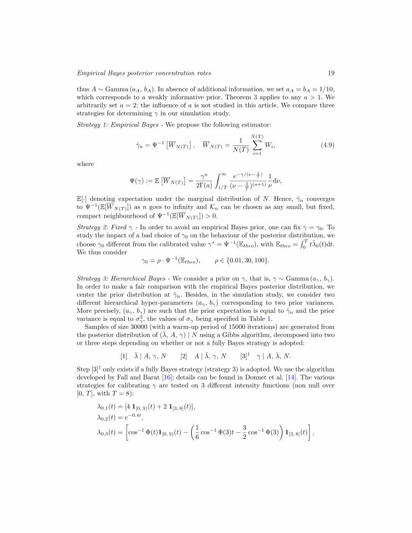
thus A ∼ Gamma (aA, bA). In absence of additional information, we set aA = bA = 1/10,which corresponds to a weakly informative prior. Theorem 3 applies to any a > 1. Wearbitrarily set a = 2; the influence of a is not studied in this article. We compare threestrategies for determining γ in our simulation study.

Strategy 1: Empirical Bayes - We propose the following estimator:

γn = Ψ−1[WN(T )

], WN(T ) =

1

N(T )

N(T )∑i=1

Wi, (4.9)

where

Ψ(γ) := E[WN(T )

]=

γa

2Γ(a)

∫ ∞1/T

e−γ/(ν−1T )

(ν − 1T )(a+1)

1

νdν,

E[·] denoting expectation under the marginal distribution of N . Hence, γn convergesto Ψ−1(E[WN(T )]) as n goes to infinity and Kn can be chosen as any small, but fixed,

compact neighbourhood of Ψ−1(E[WN(T )]) > 0.

Strategy 2: Fixed γ - In order to avoid an empirical Bayes prior, one can fix γ = γ0. Tostudy the impact of a bad choice of γ0 on the behaviour of the posterior distribution, we

choose γ0 different from the calibrated value γ∗ = Ψ−1(Etheo), with Etheo =∫ T

0tλ0(t)dt.

We thus considerγ0 = ρ ·Ψ−1(Etheo), ρ ∈ 0.01, 30, 100.

Strategy 3: Hierarchical Bayes - We consider a prior on γ, that is, γ ∼ Gamma (aγ , bγ).In order to make a fair comparison with the empirical Bayes posterior distribution, wecenter the prior distribution at γn. Besides, in the simulation study, we consider twodifferent hierarchical hyper-parameters (aγ , bγ) corresponding to two prior variances.More precisely, (aγ , bγ) are such that the prior expectation is equal to γn and the priorvariance is equal to σ2

γ , the values of σγ being specified in Table 1.Samples of size 30000 (with a warm-up period of 15000 iterations) are generated from

the posterior distribution of (λ, A, γ) | N using a Gibbs algorithm, decomposed into twoor three steps depending on whether or not a fully Bayes strategy is adopted:

[1] λ | A, γ, N [2] A | λ, γ, N [3]† γ | A, λ, N.

Step [3]† only exists if a fully Bayes strategy (strategy 3) is adopted. We use the algorithmdeveloped by Fall and Barat [16]; details can be found in Donnet et al. [14]. The variousstrategies for calibrating γ are tested on 3 different intensity functions (non null over[0, T ], with T = 8):

λ0,1(t) = [4 1[0, 3)(t) + 2 1[3, 8](t)],

λ0,2(t) = e−0.4t,

λ0,3(t) =

[cos−1 Φ(t)1[0, 3)(t)−

(1

6cos−1 Φ(3)t− 3

2cos−1 Φ(3)

)1[3, 8](t)

],

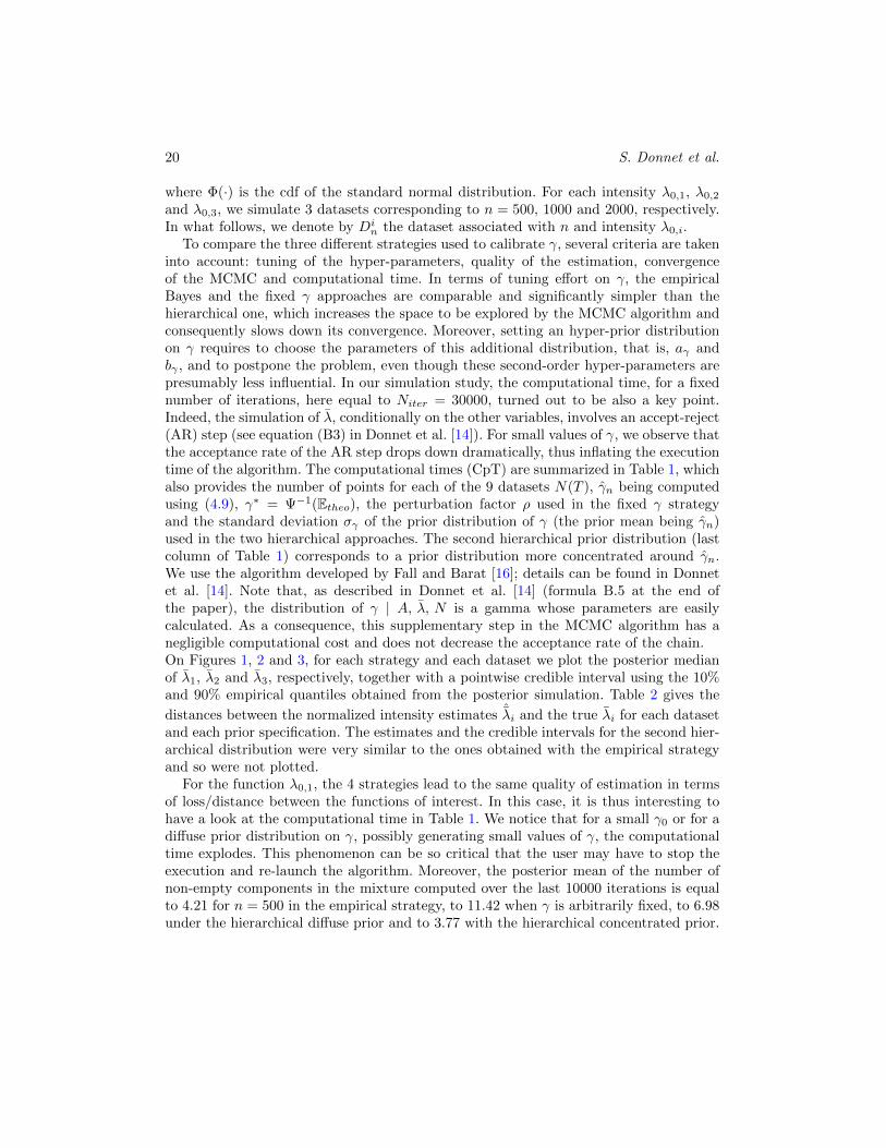
20 S. Donnet et al.

where Φ(·) is the cdf of the standard normal distribution. For each intensity λ0,1, λ0,2

and λ0,3, we simulate 3 datasets corresponding to n = 500, 1000 and 2000, respectively.In what follows, we denote by Di

n the dataset associated with n and intensity λ0,i.To compare the three different strategies used to calibrate γ, several criteria are taken

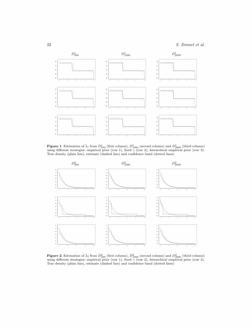
into account: tuning of the hyper-parameters, quality of the estimation, convergenceof the MCMC and computational time. In terms of tuning effort on γ, the empiricalBayes and the fixed γ approaches are comparable and significantly simpler than thehierarchical one, which increases the space to be explored by the MCMC algorithm andconsequently slows down its convergence. Moreover, setting an hyper-prior distributionon γ requires to choose the parameters of this additional distribution, that is, aγ andbγ , and to postpone the problem, even though these second-order hyper-parameters arepresumably less influential. In our simulation study, the computational time, for a fixednumber of iterations, here equal to Niter = 30000, turned out to be also a key point.Indeed, the simulation of λ, conditionally on the other variables, involves an accept-reject(AR) step (see equation (B3) in Donnet et al. [14]). For small values of γ, we observe thatthe acceptance rate of the AR step drops down dramatically, thus inflating the executiontime of the algorithm. The computational times (CpT) are summarized in Table 1, whichalso provides the number of points for each of the 9 datasets N(T ), γn being computedusing (4.9), γ∗ = Ψ−1(Etheo), the perturbation factor ρ used in the fixed γ strategyand the standard deviation σγ of the prior distribution of γ (the prior mean being γn)used in the two hierarchical approaches. The second hierarchical prior distribution (lastcolumn of Table 1) corresponds to a prior distribution more concentrated around γn.We use the algorithm developed by Fall and Barat [16]; details can be found in Donnetet al. [14]. Note that, as described in Donnet et al. [14] (formula B.5 at the end ofthe paper), the distribution of γ | A, λ, N is a gamma whose parameters are easilycalculated. As a consequence, this supplementary step in the MCMC algorithm has anegligible computational cost and does not decrease the acceptance rate of the chain.On Figures 1, 2 and 3, for each strategy and each dataset we plot the posterior medianof λ1, λ2 and λ3, respectively, together with a pointwise credible interval using the 10%and 90% empirical quantiles obtained from the posterior simulation. Table 2 gives the

distances between the normalized intensity estimates ˆλi and the true λi for each datasetand each prior specification. The estimates and the credible intervals for the second hier-archical distribution were very similar to the ones obtained with the empirical strategyand so were not plotted.

For the function λ0,1, the 4 strategies lead to the same quality of estimation in termsof loss/distance between the functions of interest. In this case, it is thus interesting tohave a look at the computational time in Table 1. We notice that for a small γ0 or for adiffuse prior distribution on γ, possibly generating small values of γ, the computationaltime explodes. This phenomenon can be so critical that the user may have to stop theexecution and re-launch the algorithm. Moreover, the posterior mean of the number ofnon-empty components in the mixture computed over the last 10000 iterations is equalto 4.21 for n = 500 in the empirical strategy, to 11.42 when γ is arbitrarily fixed, to 6.98under the hierarchical diffuse prior and to 3.77 with the hierarchical concentrated prior.

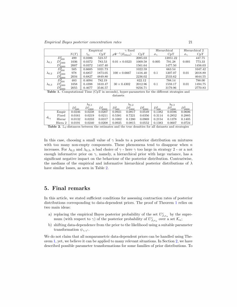
Empirical Bayes posterior concentration rates 21

Empirical γ fixed Hierarchical Hierarchical 2N(T ) γn CpT ρΨ−1(Etheo) CpT σγ CpT σγ CpT

λ0,1

D1500 499 0.0386 523.57

0.01 × 0.03232085.03

0.00512051.22

0.001447.75

D11000 1036 0.0372 783.53 1009.58 791.28 773.33

D12000 2007 0.0372 1457.40 1561.64 1477.50 1456.03

λ0,2

D2500 505 0.6605 1021.73

100 × 0.66671022.59

0.1663.54

0.011047.42

D21000 978 0.6857 1873.05 1416.40 1207.07 2018.89

D22000 2034 0.6827 4849.80 2236.02 2533.62 4644.55

λ0,3

D3500 483 0.4094 782.19

30 × 0.4302822.12

0.1788.14

0.01788.00

D31000 1058 0.4398 1610.47 2012.96 1559.17 1494.75

D32000 2055 0.4677 3546.57 9256.71 3179.96 2770.83

Table 1. Computational Time (CpT in seconds), hyper-parameters for the different strategies anddatasets

λ0,1 λ0,2 λ0,3D1

500 D11000 D1

2000 D2500 D2

1000 D22000 D3

500 D31000 D3

2000

dL1

Empir 0.0246 0.0238 0.0207 0.0921 0.0817 0.0549 0.1382 0.0596 0.0606Fixed 0.0161 0.0219 0.0211 0.5381 0.7221 0.6356 0.3114 0.2852 0.2885Hierar 0.0132 0.0233 0.0317 0.1082 0.1280 0.0969 0.2154 0.1378 0.1405Hiera 2 0.0191 0.0240 0.0208 0.0925 0.0815 0.0552 0.1383 0.0607 0.0724

Table 2. L1-distances between the estimates and the true densities for all datasets and strategies

In this case, choosing a small value of γ leads to a posterior distribution on mixtureswith too many non-empty components. These phenomena tend to disappear when nincreases. For λ0,2 and λ0,3, a bad choice of γ - here γ too large in strategy 2 - or a notenough informative prior on γ, namely, a hierarchical prior with large variance, has asignificant negative impact on the behaviour of the posterior distribution. Contrariwise,the medians of the empirical and informative hierarchical posterior distributions of λhave similar losses, as seen in Table 2.

5. Final remarks

In this article, we stated sufficient conditions for assessing contraction rates of posteriordistributions corresponding to data-dependent priors. The proof of Theorem 1 relies ontwo main ideas:

a) replacing the empirical Bayes posterior probability of the set U cJ1εn by the supre-mum (with respect to γ) of the posterior probability of U cJ1εn over a set Kn;

b) shifting data-dependence from the prior to the likelihood using a suitable parametertransformation ψγ,γ′ .

We do not claim that all nonparametric data-dependent priors can be handled using The-orem 1, yet, we believe it can be applied to many relevant situations. In Section 2, we havedescribed possible parameter transformations for some families of prior distributions. To

22 S. Donnet et al.

D1500 D1

1000 D12000

0 2 4 6 8

0.00

0.05

0.10

0.15

0.20

0 2 4 6 8

0.00

0.05

0.10

0.15

0.20

0 2 4 6 8

0.00

0.05

0.10

0.15

0.20

0 2 4 6 8

0.00

0.05

0.10

0.15

0.20

0 2 4 6 8

0.00

0.05

0.10

0.15

0.20

0 2 4 6 8

0.00

0.05

0.10

0.15

0.20

0 2 4 6 8

0.00

0.05

0.10

0.15

0.20

0 2 4 6 8

0.00

0.05

0.10

0.15

0.20

0 2 4 6 8

0.00

0.05

0.10

0.15

0.20

Figure 1. Estimation of λ1 from D1500 (first column), D1

1000 (second column) and D12000 (third column)

using different strategies: empirical prior (row 1), fixed γ (row 2), hierarchical empirical prior (row 3).True density (plain line), estimate (dashed line) and confidence band (dotted lines)

D2500 D2

1000 D22000

0 2 4 6 8

0.00.2

0.40.6

0.81.0

1.2

0 2 4 6 8

0.00.2

0.40.6

0.81.0

1.2

0 2 4 6 8

0.00.2

0.40.6

0.81.0

1.2

0 2 4 6 8

0.00.2

0.40.6

0.81.0

1.2

0 2 4 6 8

0.00.2

0.40.6

0.81.0

1.2

0 2 4 6 8

0.00.2

0.40.6

0.81.0

1.2

0 2 4 6 8

0.00.2

0.40.6

0.81.0

1.2

0 2 4 6 8

0.00.2

0.40.6

0.81.0

1.2

0 2 4 6 8

0.00.2

0.40.6

0.81.0

1.2

Figure 2. Estimation of λ2 from D2500 (first column), D2

1000 (second column) and D22000 (third column)

using different strategies: empirical prior (row 1), fixed γ (row 2), hierarchical empirical prior (row 3).True density (plain line), estimate (dashed line) and confidence band (dotted lines)

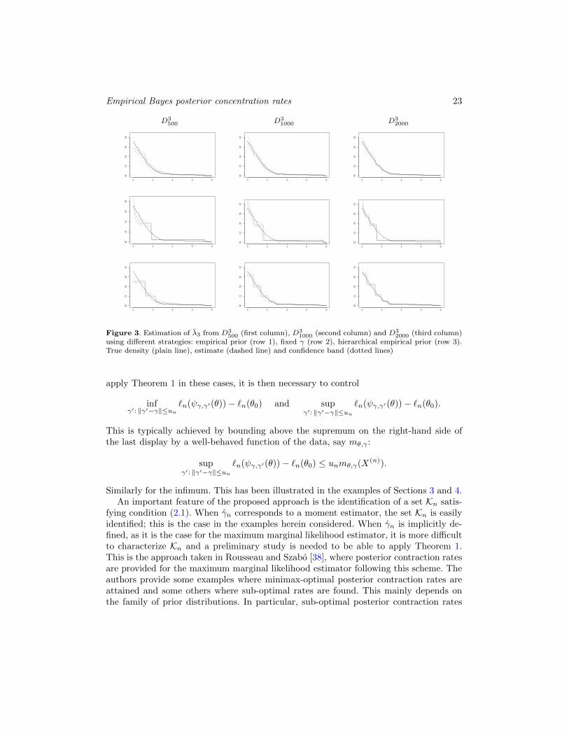
Empirical Bayes posterior concentration rates 23

D3500 D3

1000 D32000

0 2 4 6 8

0.00.2

0.40.6

0.8

0 2 4 6 8

0.00.2

0.40.6

0.8

0 2 4 6 8

0.00.2

0.40.6

0.8

0 2 4 6 8

0.00.2

0.40.6

0.8

0 2 4 6 8

0.00.2

0.40.6

0.8

0 2 4 6 8

0.00.2

0.40.6

0.8

0 2 4 6 8

0.00.2

0.40.6

0.8

0 2 4 6 8

0.00.2

0.40.6

0.8

0 2 4 6 8

0.00.2

0.40.6

0.8

Figure 3. Estimation of λ3 from D3500 (first column), D3

1000 (second column) and D32000 (third column)

using different strategies: empirical prior (row 1), fixed γ (row 2), hierarchical empirical prior (row 3).True density (plain line), estimate (dashed line) and confidence band (dotted lines)

apply Theorem 1 in these cases, it is then necessary to control

infγ′: ‖γ′−γ‖≤un

`n(ψγ,γ′(θ))− `n(θ0) and supγ′: ‖γ′−γ‖≤un

`n(ψγ,γ′(θ))− `n(θ0).

This is typically achieved by bounding above the supremum on the right-hand side ofthe last display by a well-behaved function of the data, say mθ,γ :

supγ′: ‖γ′−γ‖≤un

`n(ψγ,γ′(θ))− `n(θ0) ≤ unmθ,γ(X(n)).

Similarly for the infimum. This has been illustrated in the examples of Sections 3 and 4.An important feature of the proposed approach is the identification of a set Kn satis-

fying condition (2.1). When γn corresponds to a moment estimator, the set Kn is easilyidentified; this is the case in the examples herein considered. When γn is implicitly de-fined, as it is the case for the maximum marginal likelihood estimator, it is more difficultto characterize Kn and a preliminary study is needed to be able to apply Theorem 1.This is the approach taken in Rousseau and Szabo [38], where posterior contraction ratesare provided for the maximum marginal likelihood estimator following this scheme. Theauthors provide some examples where minimax-optimal posterior contraction rates areattained and some others where sub-optimal rates are found. This mainly depends onthe family of prior distributions. In particular, sub-optimal posterior contraction rates

24 S. Donnet et al.

are obtained for Gaussian priors in the form

θiind∼ N (0, γi−(2α+1)), i ∈ N,

when the true parameter belongs to a Sobolev ball with smoothness β > α+ 1/2.Although data-dependent prior distributions are commonly used in practice, theoreti-

cal properties have been so far considered only for maximum marginal likelihood empiricalBayes procedures when an explicit expression of the marginal likelihood is available. Thepresent contribution is an attempt at filling this gap.

Acknowledgements

This research benefited from the support of the “Chaire Economie et Gestion des Nou-velles Donnees”, under the auspices of the Institut Louis Bachelier, Havas-Media andParis-Dauphine. The research of Sophie Donnet, Vincent Rivoirard and Judith Rousseauwas partly supported by the French Agence Nationale de la Recherche (ANR 2011 BS01010 01 projet Calibration). Most of the research work of Catia Scricciolo was done whenshe was affiliated to Bocconi University, whose financial support is gratefully acknowl-edged. The authors would like to thank the Editor, an Associate Editor and two anony-mous referees whose suggestions helped to improve the final presentation of the article.

References

[1] Adams, R. P., Murray, I., and MacKay, D. J. (2009). Tractable nonparametricBayesian inference in Poisson processes with Gaussian process intensities. Proceed-ings of the 26th Annual International Conference on Machine Learning. ACM.

[2] Ahmed, S. and Reid, N. (2001). Empirical Bayes and Likelihood Inference. LectureNotes in Statistics, Springer.

[3] Andersen, P. K., Borgan, A., Gill, R. D., and Keiding, N. (1993). Statistical modelsbased on counting processes. Springer Series in Statistics. Springer-Verlag, New York.

[4] Barron, A., Schervish, M., and Wasserman, L. (1999). The consistency of posteriordistributions in nonparametric problems. Ann. Statist., 27(2):536–561.

[5] Belitser, E., Serra, P., and van Zanten, H. (2015). Rate-optimal Bayesian intensitysmoothing for inhomogeneous Poisson processes. J. Statist. Plann. Inference, 166:24–35.

[6] Berger, J. (1985). Statistical Decision Theory and Bayesian Analysis. Springer-Verlag,New York, second edition.

[7] Carroll, R. and Hall, P. (1988). Optimal rates of convergence for deconvolving adensity. J. American Statist. Assoc., 83(404):1184–1186.

[8] Casella, G. (1985). An introduction to empirical Bayes data analysis. The AmericanStatistician, 39(2):83–87.

[9] Cheng, N. and Yuan, T. (2013). Nonparametric Bayesian lifetime data analysis usingDirichlet process lognormal mixture model. Naval Res. Logist., 60(3):208–221.

Empirical Bayes posterior concentration rates 25

[10] Clyde, M. A. and George, E. I. (2000). Flexible empirical Bayes estimation forwavelets. J. Royal Statist. Society Series B, 62(4):681–698.

[11] Cui, W. and George, E. I. (2008). Empirical Bayes vs. fully Bayes variable selection.J. Statist. Plann. Inference, 138(4):888–900.

[12] Daley, D. J. and Vere-Jones, D. (2003). An introduction to the theory of pointprocesses. Vol. I. Probability and its Applications (New York). Springer-Verlag, NewYork, second edition. Elementary theory and methods.

[13] Daley, D. J. and Vere-Jones, D. (2008). An introduction to the theory of pointprocesses. Vol. II. Probability and its Applications (New York). Springer, New York,second edition. General theory and structure.

[14] Donnet, S., Rivoirard, V., Rousseau, J., and Scricciolo, C. (2014). Posterior con-centration rates for empirical Bayes procedures, with applications to Dirichlet Processmixtures. arXiv:1406.4406v1.

[15] Donnet, S., Rivoirard, V., Rousseau, J., and Scricciolo, C. (2016). Posteriorconcentration rates for counting processes with Aalen multiplicative intensities.arXiv:1407.6033v1, to appear in Bayesian Analysis.

[16] Fall, M. D. and Barat, E. (2012). Gibbs sampling methods for Pitman-Yor mixturemodels. Technical report.

[17] Fan, J. (1991a). Global behavior of deconvolution kernel estimates. Statistica Sinica,1:541–551.

[18] Fan, J. (1991b). On the optimal rates of convergence for nonparametric deconvolu-tion problems. Ann. Statist., 19(3):1257–1272.

[19] Fan, J. (1992). Deconvolution with supersmooth errors. Canadian J. Statist.,20(2):155–169.

[20] Ferguson, T. (1974). Prior distributions in spaces of probability measures. Ann.Statist., 2(4):615–629.

[21] Gaıffas, S. and Guilloux, A. (2012). High-dimensional additive hazards models andthe Lasso. Electron. J. Statist., 6:522–546.

[22] Ghosal, S., Ghosh, J. K., and van der Vaart, A. (2000). Convergence rates of pos-terior distributions. Ann. Statist., 28(2):500–531.

[23] Ghosal, S. and van der Vaart, A. (2007a). Convergence rates of posterior distribu-tions for non iid observations. Ann. Statist., 35(1):192–223.

[24] Ghosal, S. and van der Vaart, A. (2007b). Posterior convergence rates of Dirichletmixtures at smooth densities. Ann. Statist., 35(2):697–723.

[25] Ghosal, S. and van der Vaart, A. W. (2001). Entropies and rates of convergencefor maximum likelihood and Bayes estimation for mixtures of normal densities. Ann.Statist., 29(5):1233–1263.

[26] Ghosh, J. K. and Ramamoorthi, R. V. (2003). Bayesian Nonparametrics. Springer-Verlag, New York.

[27] Hansen, N. R., Reynaud-Bouret, P., and Rivoirard, V. (2015). Lasso and probabilis-tic inequalities for multivariate point processes. Bernoulli, 21(1):83–143.

[28] Hjort, N. L., Holmes, C., Muller, P., and Walker, S. G. (2010). Bayesian Nonpara-metrics. Cambridge University Press, Cambridge, UK.

[29] Karr, A. F. (1991). Point processes and their statistical inference, volume 7 of

26 S. Donnet et al.

Probability: Pure and Applied. Marcel Dekker Inc., New York, second edition.[30] Kottas, A. and Sanso, B. (2007). Bayesian mixture modeling for spatial Poisson

process intensities, with applications to extreme value analysis. J. Statist. Plann.Inference, 137(10):3151–3163.

[31] Kruijer, W., Rousseau, J., and van der Vaart, A. (2010). Adaptive Bayesian densityestimation with location-scale mixtures. Electron. J. Stat., 4:1225–1257.

[32] Lo, A. Y. (1992). Bayesian inference for Poisson process models with censored data.J. Nonparametr. Statist., 2(1):71–80.

[33] McAuliffe, J. D., Blei, D. M., and Jordan, M. I. (2006). Nonparametric empiricalBayes for the Dirichlet process mixture model. Statistics and Computing, 16(1):5–14.

[34] Petrone, S., Rousseau, J., and Scricciolo, C. (2014). Bayes and empirical Bayes: dothey merge? Biometrika, 101(2):285–302.

[35] Reynaud-Bouret, P. (2006). Penalized projection estimators of the Aalen multiplica-tive intensity. Bernoulli, 12(4):633–661.

[36] Richardson, S. and Green, P. (1997). On Bayesian analysis of mixtures with anunknown number of components (with discussion). J. Royal Statist. Society Series B,59(4):731–792.

[37] Rousseau, J. (2010). Rates of convergence for the posterior distributions of mix-tures of Betas and adaptive nonparametric estimation of the density. Ann. Statist.,38(1):146–180.

[38] Rousseau, J. and Szabo, B. T. (2015). Asymptotic behaviour of the empirical Bayesposteriors associated to maximum marginal likelihood estimator. Technical report.

[39] Salomond, J.-B. (2014). Concentration rate and consistency of the posterior dis-tribution for selected priors under monotonicity constraints. Electron. J. Statist.,8(1):1380–1404.

[40] Sarkar, A., Pati, D., Mallick, B. K., and Carroll, R. J. (2013). Adaptive posteriorconvergence rates in Bayesian density deconvolution with supersmooth errors. Tech-nical report, arXiv:1308.5427v2.

[41] Schwartz, L. (1965). On Bayes procedures. Z. Warsch. Verw. Gebiete, 4(1):10–26.[42] Scricciolo, C. (2014). Adaptive Bayesian density estimation in Lp-metrics with

Pitman-Yor or normalized inverse-Gaussian process kernel mixtures. Bayesian Anal-ysis, 9(2):475–520.

[43] Scricciolo, C. (2015). Empirical Bayes conditional density estimation. STATISTICA,LXXV(1):37–55.

[44] Serra, P. and Krivobokova, T. (2014). Adaptive empirical Bayesian smoothingsplines. Technical report.

[45] Shen, W., Tokdar, S., and Ghosal, S. (2013). Adaptive Bayesian multivariate densityestimation with Dirichlet mixtures. Biometrika, 100(3):623–640.

[46] Shen, X. and Wasserman, L. (2001). Rates of convergence of posterior distributions.Ann. Statist., 29(3):687–714.

[47] Sniekers, S. and van der Vaart, A. (2015). Adaptive Bayesian credible sets in re-gression with a Gaussian process prior. Electron. J. Statist., 9(2):2475–2527.

[48] Szabo, B., van der Vaart, A., and van Zanten, H. (2015a). Honest Bayesian confi-dence sets for the L2-norm. Journal of Statistical Planning and Inference, 166:36–51.

Empirical Bayes posterior concentration rates 27

Special Issue on Bayesian Nonparametrics.[49] Szabo, B., van der Vaart, A. W., and van Zanten, J. H. (2015b). Frequentist coverage

of adaptive nonparametric Bayesian credible sets. Ann. Statist., 43(4):1391–1428.[50] Szabo, B. T., van der Vaart, A. W., and van Zanten, J. H. (2013). Empirical Bayes

scaling of Gaussian priors in the white noise model. Electron. J. Statist., 7:991–1018.[51] Williamson, R. E. (1956). Multiply monotone functions and their Laplace trans-

forms. Duke Math. J., 23:189–207.