Potential Benefits of Discrete-Time Controller- based ... · Potential Benefits of Discrete-Time Controller-based Treatments over Protocol-based Cancer Therapies Johanna Sápi, Dániel

Acta Polytechnica Hungarica Vol. 14, No. 1, 2017

– 11 –

Potential Benefits of Discrete-Time Controller-

based Treatments over Protocol-based Cancer

Therapies

Johanna Sápi, Dániel András Drexler, Levente Kovács

Research and Innovation Center of Óbuda University, Physiological Controls

Group, Óbuda University, Kiscelli utca 82, H-1032 Budapest, Hungary

{sapi.johanna, drexler.daniel, kovacs.levente}@nik.uni-obuda.hu

Abstract: In medical practice, the effectiveness of fighting cancer is not only determined by

the composition of the used drug, but determined by the administration method as well. As

a result, having drugs with a suitable action profile is just a promising beginning, but

without appropriate delivery methods, the therapy still can be ineffective. Finding the

optimal biologic dose is an empirical process in medical practice; however, using

controllers, an automated optimal administration can be determined. In this paper, we

evaluate the effectiveness of different drug delivery protocols; using in silico simulations

(like bolus doses, low-dose metronomic regimen and continuous infusion therapy). In

addition, we compare these results with discrete-time controller-based treatments

containing state feedback, setpoint control, actual state observer and load estimation.

Keywords: antiangiogenic therapy; maximum tolerated dose; bolus dose; low-dose

metronomic regimen; continuous infusion therapy; optimal biologic dose; discrete-time

control; state feedback; setpoint control; actual state observer; load estimation

1 Introduction

1.1 Biomedical Background

Tumor cells can appear in the human body after a somatic mutation. As tumor

cells proliferate, the number of cells increase, and the tumor volume grows. This

growth, however, is limited since blood supply is provided by the nearby

capillaries, and if the tumor cells grow farther than the diffusion distance (150

μm), nutrition and oxygen access decrease. In order to overcome this problem,

tumor cells need their own blood supply. There are two main ways to form new

blood vessels. The formation of the first primitive vascular plexus is called

vasculogenesis, while the formation of new blood vessels from the preexisting

J. Sápi et al. Potential Benefits of Discrete-Time Controller-based Treatments over Protocol-based Cancer Therapies

– 12 –

microvasculature is angiogenesis [1]. In the case of tumor growth, angiogenesis

takes place, which is regulated by pro- and antiangiogenic factors. The most

important proangiogenic factor is the vascular endothelial growth factor (VEGF)

since it specifically regulates endothelial proliferation [2] which is essential for

angiogenesis. Therefore, VEGF inhibition is an important therapeutic target [3];

and to control angiogenesis, anti-VEGF agents and other VEGF inhibitors are

being used around the world [4]. However, the best angiogenic inhibition

administration method is still unknown in clinical practice [5], thus an effective

and automatic administration method is required.

1.2 Background of the Control Problem

We investigated a well-known tumor growth model under antiangiogenic therapy

[6] and designed several continuous-time controllers like an LQ control method

and state observer [7-9], flat control [10-12], modern robust control method [13-

15], feedback linearization method [16] and adaptive fuzzy techniques [17].

However, with the current scientific knowledge, there is no medical device which

can handle continuous infusion cancer therapy [18]; hence we designed a discrete-

time control herein.

2 Tumor Growth Model

P. Hahnfeldt et al. created a model which describes tumor growth under

angiogenic inhibition [6]. Assuming that after the injection, the level of the

inhibitor in the bloodstream is equal to the amount of the injected inhibitor, the

original third-order system was modified to a second-order system:

,

ln

1

22

3/2

112

2

1111

xy

gexxdxbxx

x

xxx

(1)

(2)

(3)

where the first state variable (x1) is the tumor volume [mm3], while the second

state variable (x2) is the volume of the vasculature of the tumor [mm3]. The input

of the model is the concentration of the injected inhibitor (g [mg/kg]). The first

equation contains the λ1 parameter which describes the tumor growth rate (1/day).

The change of the vasculature volume depends on three effects: a) the tumor can

stimulate the already existing capillaries to form new blood vessels by the process

of sprouting (parameter b [1/day]), b) endothelial cell death causes volume loss in

vasculature (parameter d [1/(day·mm2]), c) the administration of antiangiogenic


– 13 –

drug causes volume loss in vasculature as well (parameter e [kg/(day·mg]). In the

case of Lewis lung carcinoma, and using endostatin as antiangiogenic drug, the

parameters are the following [1]: λ1 = 0.192 1/day, b = 5.85 1/day, d = 0.00873

1/day·mm2, e = 0.66 kg/(day·mg).

3 Protocol-based Cancer Therapies

3.1 Cancer Protocols in the Light of the Dosage Problem

As it was discussed previously, there is no best way for antiangiogenic drug

administration in clinical practice. There are three main methods which are used;

however, both ones have advantages and disadvantages. Bolus dose (BD)

administration means that the patient receives drug boluses on given days, and

between the injections, the treatment has rest periods when there is no drug

administration at all. The amount of injected dose can be the Maximum Tolerated

Dose (MTD) or any lower dose. After an MTD injection, the treatment should

include an extended rest period in order to avoid adverse events. Instead of bolus

doses, anticancer drugs can be delivered over prolonged periods using low-doses,

this therapy is called as Low-Dose Metronomic (LDM) regimen. Of course, in this

case the rest periods can be shorter; but the real question is to find the Optimal

Biologic Dose (OBD) which results in the best therapeutic efficacy. Finally, in

clinical environment continuous infusion therapy is feasible (e.g. using mini-

osmotic pumps), but there is no portable device yet. Clinical experiments have

shown that low-dose administration therapies have better therapeutic efficacy than

bolus dose injections, and continuous infusion therapies have even better results

[19].

3.2 Simulation Results of the Protocol-based Cancer Therapies

The effect of bolus dose administration, low-dose metronomic regimen and

continuous infusion therapy was investigated in silico, using the modified

Hahnfeldt-model described by Eq. (1)-(3). The total administered inhibitor

concentration is 300 mg/kg, and treatment period is 15 days in every simulation,

in order to get comparable results. Simulations start from the lethal steady-state of

the model when the initial value of tumor volume (x1(0)) and vascular volume

(x2(0)) are 1.734∙104

mm3. Four different scenarios were examined [20] (left side

of Figure 1).


– 14 –

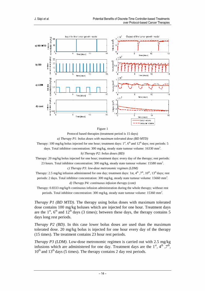
Figure 1

Protocol based therapies (treatment period is 15 days)

a) Therapy P1: bolus doses with maximum tolerated dose (BD MTD)

Therapy: 100 mg/kg bolus injected for one hour; treatment days: 1st, 6th and 12th days; rest periods: 5

days. Total inhibitor concentration: 300 mg/kg, steady state tumour volume: 16330 mm3.

b) Therapy P2: bolus doses (BD)

Therapy: 20 mg/kg bolus injected for one hour; treatment days: every day of the therapy; rest periods:

23 hours. Total inhibitor concentration: 300 mg/kg, steady state tumour volume: 15580 mm3.

c) Therapy P3: low-dose metronomic regimen (LDM)

Therapy: 2.5 mg/kg infusion administered for one day; treatment days: 1st, 4th ,7th, 10th, 13th days; rest

periods: 2 days. Total inhibitor concentration: 300 mg/kg, steady state tumour volume: 15660 mm3.

d) Therapy P4: continuous infusion therapy (cont)

Therapy: 0.8333 mg/kg/h continuous infusion administration during the whole therapy; without rest

periods. Total inhibitor concentration: 300 mg/kg, steady state tumour volume: 15360 mm3.

Therapy P1 (BD MTD). The therapy using bolus doses with maximum tolerated

dose contains 100 mg/kg boluses which are injected for one hour. Treatment days

are the 1st, 6

th and 12

th days (3 times); between these days, the therapy contains 5

days long rest periods.

Therapy P2 (BD). In this case lower bolus doses are used than the maximum

tolerated dose. 20 mg/kg bolus is injected for one hour every day of the therapy

(15 times). The treatment contains 23 hour rest periods.

Therapy P3 (LDM). Low-dose metronomic regimen is carried out with 2.5 mg/kg

infusions which are administered for one day. Treatment days are the 1st, 4

th ,7

th,

10th

and 13th

days (5 times). The therapy contains 2 day rest periods.


– 15 –

Therapy P4 (cont). Continuous infusion therapy is carried out with

0.8333 mg/kg/h continuous infusion during the whole treatment, without rest

periods.

The right side of Figure 1 depicts the outputs of the tumor growth model, using

Therapy P1 - Therapy P4 as inputs. Similarly to the clinical experimental results,

simulations show that the less effective therapy is the bolus doses with maximum

tolerated dose (BD MTD). Tumor volume reduction is not effective (steady state

tumor volume is 16330 mm3), and beside this, side-effects can occur and quality

of life (QoL) of the patient decreases due to the therapy. Lower bolus doses (BD)

cause continuous slight reduction of the tumor volume, however this is not

significant (steady state tumor volume is 15580 mm3). Another disadvantage of

this method is the resulting high frequency oscillation-like characteristics of the

vascular volume. Low-dose metronomic administration (LDM) has similar results

as BD in terms of tumor volume reduction (steady state tumor volume is

15660 mm3) and oscillation-like characteristics of the vascular volume; however,

the oscillation frequency and amplitude are lower which can be more tolerable for

the patient. The most effective treatment is the continuous infusion therapy (cont)

since it results in the lower steady state tumor volume (15360 mm3) and the

change of the vascular volume is a smooth curve. In addition, due to the extremely

low dosage, continuous infusion therapy has virtually no side-effects.

4 Discrete-Time Controller-based Treatments

The modified Hahnfeldt-model describes a nonlinear system, which has to be

linearized due to controller design aspects. We applied operating point

linearization in the g0 = 0 operating point. The resulting LTI (linear time

invariant) system using state space representation is

,DuCxy

BuAxx

(4)

(5)

where the matrices are

3

2

123

1

1

2

111

2

11

3

2

log

xdxxdb

x

x

x

x

A

(6)


– 16 –

.0

01

0

2

D

C

ex

B

(7)

(8)

(9)

4.1 Discrete-Time Controller Design with State Feedback,

Setpoint Control, Actual State Observer and Load

Estimation

Taking into account a feasible discrete-time system, the state space equations are

.

1

ii

ididi

Cxy

uBxAx

(10)

(11)

The controllability and observability matrices of the discrete-time system are

,

...

]...[

1

1

n

d

d

O

d

n

ddddC

CA

CA

C

M

BABABM

(12)

(13)

where n is the dimension of the state variables. Since for every nonzero operating

point, the matrices are full rank, the system is controllable and observable in every

operating point.

In order to find optimal solutions, we used the LQ control method as state

feedback to minimize the tumor volume (x1) using the lowest possible control

signal. The discrete-time cost function containing the positive definite Q and R

weighting matrices is

T

i

i

T

ii

T

i RuuQxxuJ1

.)( (14)

As our aim was to minimize the square of the output (x12 = y

2), the Q matrix is the

following:

.CCQ T (15)


– 17 –

The sought K feedback matrix of the discrete-time LQ problem can be found using

the P solution of the Discrete Control Algebraic Ricatti Equation (DARE):

d

T

dd

T

d PABPBBRK1

(16)

.1

QPABPBBRPBAPAAP d

T

dd

T

dd

T

dd

T

d

(17)

For setpoint control, we assume that the reference signal is constant. The control

structure is needed to be extended by two matrices (Nx and Nu) in order to use

nonzero reference signal. The values of these matrices can be calculated as

follows:

,

0

0

1

m

nxmdd

u

x

IC

BIA

N

N (18)

where n is the dimension of the state variables, while m is the dimension of the

inputs (and outputs).

As the vascular volume is non-measurable, we designed an actual state observer to

estimate this state variable. We have verified that the matrix MoAd is full rank, thus

the discrete-time system is observable with an actual observer described by the

following difference equation:

.ˆˆ11 iiii HuGyxFx (19)

The F, H and G parameter matrices of the observer can be calculated as follows:

,,e 1T

n

TT

dF

T

d

T

d

T

dc

dd

dd

ACAAMG

GCBBH

GCAAF

(20)

(21)

(22)

where φF(AdT) refers to the characteristic polynomial of the matrix F evaluated at

the matrix AdT.

Assuming that a disturbance reduced to the input of the system can occur (load

change), we designed load estimation as well. The system was extended by the

disturbance modeled as a constant state-variable that adds up to the input of the

original model. The state feedback and the setpoint control were designed for the

original system; however, the actual state observer was designed for the extended

system. As a consequence, the difference equation of the state observer is

,~~

ˆ

ˆ~

ˆ

ˆ1

1

1

ii

id

i

id

iuHyG

x

xF

x

x (23)

where dx̂ is the estimation of the disturbance.


– 18 –

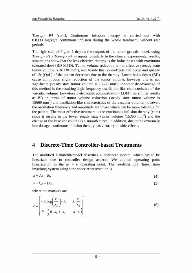
Figure 2 depicts the whole block diagram of the closed-loop discrete-time control

system containing state feedback, setpoint control, actual state observer and load

estimation. Please note that saturation is used before the input of the tumor model

in order to avoid negative or too high input values due to physiological aspects.

Figure 2

Block diagram of the discrete-time control containing state feedback, setpoint control, actual state

observer and load estimation

4.2 Simulation Results of the Discrete-Time Controller-based

Treatments

Using discrete-time controller, the treatment can contain bolus doses, low-dose

metronomic parts and continuous periods as well. In order to get comparable

results with the protocol based therapies, the treatment period was chosen to be 15

days. Parameters of the discrete-time controllers were chosen according to [21].

The operating point of the linearization is x1= x2=10 mm3, the R weighting matrix

used in the design of the LQ control is 1. In order to get steady state tumor

volumes close the protocol based cancer therapies’ values, the reference signal is

13000 mm3. Since protocol based cancer therapies do not have disturbance, the

disturbance is 0% in the case of discrete-time controllers. Three different

scenarios were examined in the light of the saturation level (left side of Figure 3).


– 19 –

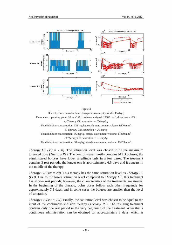
Figure 3

Discrete-time controller based therapies (treatment period is 15 days)

Parameters: operating point: 10 mm3; R: 1; reference signal: 13000 mm3; disturbance: 0%.

a) Therapy C1: saturation = 100 mg/kg

Total inhibitor concentration: 138 mg/kg, steady state tumour volume: 9870 mm3.

b) Therapy C2: saturation = 20 mg/kg


c) Therapy C3: saturation = 2.5 mg/kg


Therapy C1 (sat = 100). The saturation level was chosen to be the maximum

tolerated dose (Therapy P1). The control signal mostly contains MTD boluses; the

administered boluses have lower amplitude only in a few cases. The treatment

contains 3 rest periods, the longer one is approximately 6.5 days and it appears in

the middle of the therapy.

Therapy C2 (sat = 20). This therapy has the same saturation level as Therapy P2

(BD). Due to the lower saturation level compared to Therapy C1, this treatment

has shorter rest periods; however, the characteristics of the treatments are similar.

In the beginning of the therapy, bolus doses follow each other frequently for

approximately 7.5 days, and in some cases the boluses are smaller than the level

of saturation.

Therapy C3 (sat = 2.5). Finally, the saturation level was chosen to be equal to the

input of the continuous infusion therapy (Therapy P3). The resulting treatment

contains only one rest period in the very beginning of the treatment. After that a

continuous administration can be obtained for approximately 8 days, which is


– 20 –

followed by a phase where bolus doses follow each other frequently (the

amplitude of these boluses is the saturation level in every case).

The right side of Figure 3 depicts the outputs of the tumor growth model, using

Therapy C1 - Therapy C3 as inputs. Using Therapy C1, the total inhibitor

concentration is 138 mg/kg, which is the highest total drug administration among

the discrete-time controller based therapies. The achieved “steady state”1 tumor

volume is 9870 mm3 (since at the end of the treatment, an undershoot can be

observed). The total inhibitor concentration in Therapy C2 is 56 mg/kg, which is

substantially lower in comparison with Therapy C1; however the steady state

tumor volume is comparable (11360 mm3). Finally, Therapy C3 has resulted in the

lowest total inhibitor concentration (30 mg/kg), and the achieved steady state

tumor volume is 13153 mm3 in this case.

Conclusions

The efficacy of the therapies are compared and evaluated based on the achieved

total inhibitor concentrations and steady state tumor volumes (Figure 4). During

the protocol based therapies, the same amount of inhibitor was administered in

total. As a consequence, the comparison is quite trivial: the smaller the steady

state tumor volume, the better the therapy. Bolus doses with maximum tolerated

dose (BD MTD) is the less effective treatment; bolus doses with lower boluses

(BD) and low-dose metronomic regimen (LDM) are better; however, the best

method is the continuous infusion therapy (cont) from the protocol based

therapies. Nevertheless, discrete-time controller based therapies show better

performance regardless of the saturation value. The choice between these

therapies depends on the medical preferences and constraints. Having a patient

who can tolerate MTD, and knowing that the aim is the fastest tumor reduction,

we have to choose 100 mg/kg saturation (sat = 100). If we would like to find a

trade-off solution, 20 mg/kg saturation (sat = 20) is the most appropriate choice.

However, if slower tumor reduction is desired and/or patient does not tolerate the

inhibitor well, our choice is the 2.5 mg/kg saturation level (sat = 20).

1 In fact, in most of the cases the output of the tumor growth model does not reach the

steady state at the end of the simulation; however, as we would like to express the

effectiveness of the control in terms of tumor reduction, we use the “steady state” for

the final state of the investigated control and we specify its value.


– 21 –

Figure 4

Comparison of the therapies as functions of total inhibitor concentration and steady state tumour

volume

Protocol based therapies: bolus doses with maximum tolerated dose (BD MTD), bolus doses (BD),

low-dose metronomic regimen (LDM), continuous infusion therapy (cont). Discrete controller based

therapies: saturation: 100 mg/kg (sat = 100), saturation: 20 mg/kg (sat = 20),

saturation: 2.5 mg/kg (sat = 2.5).

Acknowledgement

This project has received funding from the European Research Council (ERC)

under the European Union’s Horizon 2020 research and innovation programme

(grant agreement No 679681).

References

[1] J. H. Distler, A. Hirth, M. Kurowska-Stolarska, R. E. Gay, S. Gay, O.

Distler, “Angiogenic and Angiostatic Factors in the Molecular Control of

Angiogenesis”, The Quarterly Journal of Nuclear Medicine, Vol. 47(3), pp.

149-161, 2003

[2] N. Ferrara, “Vascular Endothelial Growth Factor and the Regulation of

Angiogenesis”, Recent Prog Horm Res, Vol. 55, pp. 15-35, discussion 35-

36, 2000

[3] A. L. Harris, “Angiogenesis as a New Target for Cancer Control”,

European Journal of Cancer Supplements, Vol. 1, pp. 1-12, 2003


– 22 –

[4] S. Saha, M. K. Islam, J. A. Shilpi, S. Hasan, “Inhibition of VEGF: a Novel

Mechanism to Control Angiogenesis by Withania Somnifera's Key

Metabolite Withaferin A”, In Silico Pharmacol, Vol. 29, pp. 1-11, DOI:

10.1186/2193-9616-1-11, eCollection 2013

[5] O. Distler, M. Neidhart, R. E. Gay, S. Gay, “The Molecular Control of

Angiogenesis”, International Reviews of Immunology, Vol. 21(1), pp. 33-

49, 2002

[6] P. Hahnfeldt, D. Panigrahy, J. Folkman, and L. Hlatky, “Tumor

Development under Angiogenic Signaling: A Dynamical Theory of Tumor

Growth, Treatment Response, and Postvascular Dormancy”, Cancer

Research, Vol. 59, pp. 4770-4775, 1999

[7] D. A. Drexler, L. Kovács, J. Sápi, I. Harmati, Z. Benyó, “Model-based

Analysis and Synthesis of Tumor Growth under Angiogenic Inhibition: a

Case Study.” IFAC WC 2011 – 18th

World Congress of the International

Federation of Automatic Control, pp. 3753-3758, August 2011, Milano,

Italy

[8] J. Sápi, D. A. Drexler, I. Harmati, Z. Sápi, L. Kovács, “Linear State-

Feedback Control Synthesis of Tumor Growth Control in Antiangiogenic

Therapy,” SAMI 2012 – 10th IEEE International Symposium on Applied

Machine Intelligence and Informatics, pp. 143-148, January 2012, Herlany,

Slovakia

[9] J. Sápi, D. A. Drexler, I. Harmati, Z. Sápi, L. Kovács, “Qualitative Analysis

of Tumor Growth Model under Antiangiogenic Therapy – Choosing the

Effective Operating Point and Design Parameters for Controller Design,”

Optimal Control Applications and Methods, Article first published online: 9

SEP 2015, DOI: 10.1002/oca.2196

[10] D. A. Drexler, J. Sápi, A. Szeles, I. Harmati, A. Kovács, L. Kovács, “Flat

Control of Tumor Growth with Angiogenic Inhibition”, SACI 2012 – 6th

IEEE International Symposium on Applied Computational Intelligence and

Informatics, pp. 179-183, May 2012, Timisoara, Romania

[11] D. A. Drexler, J. Sápi, A. Szeles, I. Harmati, L. Kovács, “Comparison of

Path Tracking Flat Control and Working Point Linearization Based Set

Point Control of Tumor Growth with Angiogenic Inhibition”, Scientific

Bulletin of the ”Politehnica” University of Timisoara, Transactions on

Automatic Control and Computer Science, Vol. 57 (71):(2), pp. 113-120,

2012

[12] A. Szeles, D. A. Drexler, J. Sápi, I. Harmati, L. Kovács, “Study of Modern

Control Methodologies Applied to Tumor Growth under Angiogenic

Inhibition”, IFAC WC 2014 – 19th

World Congress of the International

Federation of Automatic Control, pp. 9271-9276, August 2014, Cape

Town, South Africa


– 23 –

[13] A. Szeles, J. Sápi, D. A. Drexler, I. Harmati, Z. Sápi, and L. Kovács,

“Model-based Angiogenic Inhibition of Tumor Growth using Modern

Robust Control Method”, IFAC BMS 2012 – 8th

IFAC Symposium on

Biological and Medical Systems, pp. 113-118, August 2012, Budapest,

Hungary

[14] J. Sápi, D. A. Drexler, L. Kovács, “Parameter Optimization of H∞

Controller Designed for Tumor Growth in the Light of Physiological

Aspects”, CINTI 2013 – 14th

IEEE International Symposium on

Computational Intelligence and Informatics, pp. 19-24, November 2013,

Budapest, Hungary

[15] L. Kovács, A. Szeles, J. Sápi, D. A. Drexler, I. Rudas, I. Harmati, Z. Sápi,

“Model-based Angiogenic Inhibition of Tumor Growth using Modern

Robust Control Method”, Computer Methods and Programs in

Biomedicine, Vol. 114, pp. 98-110, 2014

[16] A. Szeles, D. A. Drexler, J. Sápi, I. Harmati, Z. Sápi, L. Kovács, “Model-

based Angiogenic Inhibition of Tumor Growth using Feedback

Linearization”, CDC 2013 – 52nd

IEEE Conference on Decision and

Control, pp. 2054-2059, December 2013, Florence, Italy

[17] A. Szeles, D. A. Drexler, J. Sápi, I. Harmati, L. Kovács, “Model-based

Angiogenic Inhibition of Tumor Growth using Adaptive Fuzzy

Techniques”, Periodica Polytechnica: Electrical Engineering and

Computer Science, Vol. 58:(1), pp. 29-36, 2014

[18] J. Sápi, L. Kovács, D.A. Drexler, P. Kocsis, D. Gajári, Z. Sápi, “Tumor

Volume Estimation and Quasi-Continuous Administration for Most

Effective Bevacizumab Therapy”, Plos One, Vol. 10:(11), Paper e0142190.

20 p, 2015

[19] O. Kisker, CM. Becker, D. Prox, M. Fannon, R. D'Amato, E. Flynn, WE.

Fogler, BK. Sim, EN. Allred, SR. Pirie-Shepherd, J. Folkman, “Continuous

Administration of Endostatin by Intraperitoneally Implanted Osmotic Pump

Improves the Efficacy and Potency of Therapy in a Mouse Xenograft

Tumor Model”, Cancer Res, Vol. 61(20), pp. 7669-7674, 2001

[20] J. Sápi, D. A. Drexler, L. Kovács, “Comparison of Protocol-based Cancer

Therapies and Discrete Controller-based Treatments in the Case of

Endostatin Administration”, SMC 2016 - IEEE International Conference on

Systems, Man, and Cybernetics, pp. 3830-3835, October 2016, Budapest,

Hungary

[21] J. Sápi, D. A. Drexler, L. Kovács, “Discrete Time State Feedback with

Setpoint Control, Actual State Observer and Load Estimation for a Tumor

Growth Model”, SACI 2016 - IEEE 11th

International Symposium on

Applied Computational Intelligence and Informatics, pp. 111-118, May

2016, Timisoara, Romania

Documents

Potential Benefits of Discrete-Time Controller- based ... · Potential Benefits of Discrete-Time Controller-based Treatments over Protocol-based Cancer Therapies Johanna Sápi, Dániel