Potential Economic Effects on the Philippines of the Trans … · Potential Economic Effects on the Philippines of the Trans-Pacific Partnership (TPP)* Caesar B. Cororaton and David

Potential Economic Effects on the Philippines of the Trans-Pacific

Partnership (TPP)*

Caesar B. Cororaton and David Orden**

Revised February 2015

GII Working Paper No. 2014-1

Keywords: Trans-Pacific Partnership, Regional trade, Philippines, Global CGE

JEL Classification: C68, D58, F15

__________________________ * Research funding provided by the Global Issues Initiative/ Institute for Society, Culture and Environment, Virginia

Polytechnic Institute and State University.

**Caesar Cororaton ([email protected]) is Senior Research Fellow and David Orden ([email protected]) is Director, at the

Global Issues Initiative (GII), Institute for Society, Culture and Environment (ISCE), Virginia Polytechnic Institute

and State University. 900 N. Glebe Road, Arlington Virginia, USA, 22203.

mailto:[email protected]

mailto:[email protected]

Trans-Pacific Partnership - Philippines

1

Abstract

The TPP is a potential economic block in Asia Pacific. If the negotiations are successful, the TPP

can have important implications for the Philippines whether it decides to join or not because

countries in TPP are important markets for Philippine exports and sources of imports, investments,

and technology. The paper simulates a reduction in trade barriers within the TPP using a global

CGE model. The results indicate trade creation within the TPP and trade diversion from the non-

TPP. Philippine non-participation will generate small negative effects on the economy, but the

economic opportunity cost of non-participation is larger. If the inflows of investments into the

country improve with participation, the welfare gain is higher. While higher investments lead to

real exchange rate appreciation, the majority of Philippine sectors benefit from the scale

production effect of larger capital inflows.


2

I. Introduction

The goal of the twelve-nation Trans-Pacific Partnership (TPP) is to expand trade and

investment across the Asia Pacific region through the elimination of tariffs and non-tariff barriers

(NTBs), the harmonization of trade regulations, and the elimination of investment barriers. The

TPP group includes Brunei, Chile, New Zealand, Singapore, United States, Japan, Canada,

Mexico, Peru, Australia, Malaysia, and Vietnam. Together, this group is a huge economic block

representing 40 percent of the world’s gross domestic product (GDP) and 40 percent of world

trade. In 2012, the TPP member countries had a combined population of 783.6 million and GDP

of US$27.5 trillion. Although a TPP agreement is yet to be achieved with the members working

to resolve many challenging and contentious issues, South Korea and Taiwan have already

signified interest in joining because of the significance of the group as a major economic block1.

The Philippines has yet to signify interest in joining TPP, but the government is in the process of

evaluating a possible participation.

Based on the 10th November 2014 TPP Trade Minister’s Report to Leaders, the

negotiations among the participating countries are moving forward to finalize an agreement in

several areas including: a comprehensive market access (duty-free access to goods within the TPP

and lifting of restrictions on services, investment and financial services, temporary entry of

business persons, and government procurement); a regional agreement (common rules of origin,

trade facilitation, and elimination of non-tariff barriers); new trade issues (rules that ensure private

sector businesses can compete with State-owned enterprises on a level playing field); and cross-

cutting trade issues (promotion of small-and medium-sized enterprises, transparency and good

1 See Krist (2013) for a discussion of the early negotiations and Fergusson and Vaughn (2010) for an overview of the

TPP.


3

governance, strengthen anti-corruption efforts, improve opportunities for women and low-income

individuals, capacity building in developing countries)2.

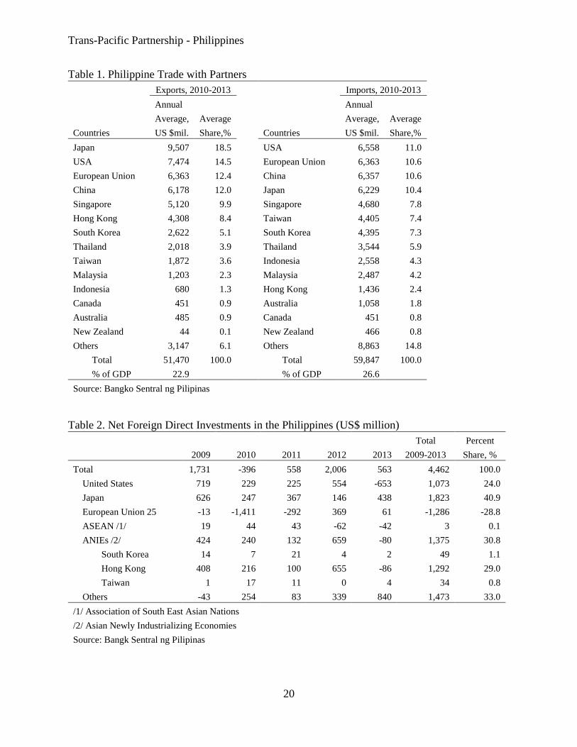
Currently, several of the key TPP member countries are important markets for Philippine

exports and sources of imports (Table 1), foreign direct investments (Table 2) and technology.

With total merchandize exports 21.1 percent of GDP and imports 24.1 percent, external trade is a

key component of the Philippine economy. Of the total exports, manufactures account for 86

percent, agriculture (including forestry) 7 percent and mining (including petro products) 5 percent.

The leading export items of the Philippines are electronics and related products which accounted

for an average share of 55 percent of total exports in 2010-2012. Raw materials and intermediate

goods accounted for 51 percent of Philippine merchandise imports in 2010-2012. The other major

import items are oil and fuel (19 percent), capital goods (17 percent), and consumer goods (12

percent). Thus, Philippine participation or non-participation in the TPP can affect its economy

because it can expand or contract existing trade and investment linkages with partners participating

in the group. Moreover, an important element in the TPP is the establishment of an institution that

monitors the compliance of participating countries to the agreed rules and regulations and settles

trade disputes. Should the Philippines decide to join the group, the institutional set-up in the TPP

can provide discipline and therefore speed up trade reforms in agriculture, investments and

corporate taxation.

The objective of this paper is to provide a quantitative analysis of the potential economic

effects on the Philippine economy of a possible TPP and whether it is a member or not. In the

analysis, a global computable general equilibrium (CGE) model (Robichaud, et al., 2011)

2 http://www.ustr.gov/about-us/press-office/press-releases/2014/November/Trans-Pacific-Partnership-Trade-

Ministers-Report-to-Leaders

http://www.ustr.gov/about-us/press-office/press-releases/2014/November/Trans-Pacific-Partnership-Trade-Ministers-Report-to-Leaders

http://www.ustr.gov/about-us/press-office/press-releases/2014/November/Trans-Pacific-Partnership-Trade-Ministers-Report-to-Leaders


4

calibrated to the GTAP 8 database3 is used to simulate the possible effects on members, non-

members and specifically the Philippine economy under three scenarios: Philippines not a TPP

member; Philippine TPP participation with no additional foreign direct investment (FDI) inflow

effects in the country; and Philippine TPP participation with additional FDI inflow effects in the

country. In the analysis, a TPP agreement will involve a 10-year phased reduction in tariffs and

NTBs among the participating parties.

There are a few quantitative assessment studies conducted that have used global CGE

models to analyze the potential economic effects of the TPP agreement. Petri, Plummer, and Zhai

(2012) calibrated the global CGE model of Zhai (2008) using a preliminary release version of the

GTAP 8 database and analyzed trade liberalization within TPP in the context of other trade

initiatives in Asia. In the analysis, changes in tariffs (including the reduction in preferential tariffs

and the utilization rate of preferences) and non-tariff barriers were considered. Itakura and Lee

(2012) used the dynamic GTAP model of Ianchovichina and Walmsley (2012) calibrated to the

GTAP 7 database analyzed trade liberalization (reduction in tariffs and non-tariff barriers) within

the TPP and within the current trade negotiations in the region. Both studies find steady and

increasing gains over time among participating nations. Using the dynamic GTAP model

calibrated to the GTAP 8 database, Cheong (2013) analyzed the potential effects of trade

liberalization within the TPP and found that not all TPP member countries would benefit from the

liberalization. Some countries would have negative GDP effects. Non-TPP countries will face

economic losses from trade diversion.

To further develop these results, and with specific focus on the Philippines, the paper is

organized as follows. The next section gives a brief discussion of the Philippines-TPP model, the

3 GTAP refers to the Global Trade Analysis Project (https://www.gtap.agecon.purdue.edu/databases/).

https://www.gtap.agecon.purdue.edu/databases/


5

tariff and NTB issues we assume TPP will address, and performance of the Philippines of attracting

foreign investment. The simulation scenarios designed around these circumstances are described.

The third section presents the simulation results including effects of a TPP on aggregate trade and

welfare among members and non-members, effects of the scenarios on output in the Philippines

disaggregate into 15 sectors and effects on factor returns for the Philippines. The final section is a

brief summary and discussion of the results.

II. Framework of Analysis

Philippines-TPP CGE model. The Robichaud, et al. (2011) model was calibrated to the

GTAP 8 database which consists of fifty seven sectors in one hundred and twenty nine

countries/regions. The database includes two types of labor (skilled and unskilled), capital, land,

and natural resources. However, to facilitate the computation of the model solution and the analysis

of results, the database was aggregated to fifteen sectors in twenty countries/regions (Table 3)4.

The fifteen sectors reflect the disaggregation of important sectors in the Philippine economy

including the labor-intensive service sector, the electronic equipment sector which produces the

country’s key exports, the agricultural crops and food manufacturing sectors which have the

highest trade barriers, and the labor-intensive textile and wearing apparel sectors which are among

the list of industries in the export promotion program of the Philippine government.

In terms of the countries/regions, eleven of the included countries are the TPP members5.

South Korea and Taiwan are included in the model because of their announced interest in the TPP.

Indonesia and Thailand are included because they are important countries in the region,

particularly in the ASEAN, and similarly to the Philippines, these countries are currently

4 Appendix A presents a mapping of the 15 sectors and 20 countries/regions to the GTAP 8 database. 5 Brunei was excluded in the model because it is not in the GTAP 8 database. The model’s sectoral and regional

aggregation compared to the GTAP 8 database is available from the authors.


6

performing due diligence on the TPP to assess the potential benefits and the domestic policy

adjustments required should they decide to join in the coming years. In addition, other main

geographic regions are aggregated into the EU25, Latin America (excluding Chile, Mexico and

Peru), Africa and a remaining Rest of the World.

Model Structure. The detailed specification of the model is given in Appendix A. Important

features of the model include: (a) a three-level production structure where value added and

intermediate inputs are used in fixed proportion to produce output and the second and third levels

are constant elasticity of substitution (CES) functions of various disaggregated factor inputs; (b)

a linear expenditure system demand structure; (c) domestically produced and imported goods are

imperfect substitutes and modeled using CES function; (d) imports of each commodity are

disaggregated using another CES function to the various sources of imports, which implies

product differentiation among imports from the various origins; (e) exports of each commodity

are disaggregated using constant elasticity of transformation (CET) function to the various export

destinations, which also implies imperfect substitutability among exports to the destinations; and

(f) the system of prices in the model reflects the cost of production plus a series of mark-ups

which consists of layers of taxes and international transport margins.

Trade Barriers. The sectoral tariff rates applied by each country/region on imports from

each of the import origins were calibrated from the GTAP 8 database. Over the past couple of

decades the series of tariff reduction programs implemented globally under the World Trade

Organization (WTO), regionally under the various regional trading agreements or unilaterally

have lowered quite considerably the level of tariff rates across countries. However, despite the

trade reform programs, tariff rates in a few commodities remain high, especially those goods that

fall under the special product categories. Furthermore, there are various NTBs which continue to


7

affect the flow of commodities across borders. In the international market for food for example,

although most of the production, processing, and distribution of food is done by the private sector,

the market is affected by various forms of government regulation. The economic justifications for

a government role in food markets stem from both the public goods aspects of disease and pest

control and the opportunities to reduce market transactions cost for firms and consumers, but

NTMs can also serve protectionist purposes (Josling, Roberts, and Orden, 2004). To factor in

some of these features in international trade into the analysis, and in an effort to capture the overall

level of protection imposed by countries on imports, the calibrated import tariff rates were

augmented to include estimates of NTBs effects available in the literature.

Modeling NTBs within a CGE framework is complex because NTBs have both demand-

shifting and supply-shifting effects which may affect both the demand and supply elasticities

which are difficult to implement in a CGE framework (Fugazza and Maur, 2008)6. Setting aside

these challenging modeling issues on NTBs, the analysis includes the estimates of NTB effects

of Kee, Nicita, and Olarreaga (2006) added to the calibrated sectoral tariff rates to come up with

the estimates of the overall level of protection. That is, following Kee, Nicita, and Olarreaga

(2006), the overall protection is 𝑇𝑖,𝑧 = 𝐴𝑉𝐸𝑖,𝑧 + 𝑡𝑖,𝑧 where 𝑇𝑖,𝑧 is the overall protection that

country z imposes on commodity imports i; 𝐴𝑉𝐸𝑖,𝑧 is the tariff ad-valorem equivalent (AVE) of

NTBs that country z imposes on imports i; and 𝑡𝑖,𝑧 is the applied tariff. The estimates of the AVE

protection used in the analysis are given in Table 4 for three aggregates of sectors. As shown, the

AVE of NTBs generally exceed the simple average tariffs reported by Kee, Nicita, and Olarreaga

(2006). In the simulations, estimates of the AVE of NTBs for agriculture in each of the

6 For example, requirements to provide information to consumers (e.g., labelling) may affect supply by changing the

costs of production and distribution but also affect consumer behavior and therefore consumer demand. Similarly,

preventing the sale of products that have hazardous effects on health or creating standards to increase compatibility

can affect both supply and demand.


8

countries/regions was applied to crops and other agriculture sectors in the model, and the

manufacturing rate to all manufacturing sectors, i.e., from food manufacturing to all other

manufacturing sectors. The estimates of the AVE of NTBs for mining was applied to the mining

sector in the model.

Foreign Investments. One of the benefits of participating in trade agreements is the

expected increase in the volume of trade flows among the participating parties as trade barriers

are minimized. Another benefit that normally goes with higher volume of trade is higher

investment flows and active transfer of technology among the participating parties. The

Philippines is located in a dynamic zone in Asia where a rapid increase in inflows of FDI has been

observed. Unfortunately, the inflows of FDI into the Philippines have been low; the country has

been underperforming in terms of attracting FDI. Using a concept called global FDI frontier, Petri,

Plummer, and Zhai (2012) have shown that the stock of FDI inflows as of 2006 into the

Philippines were significantly below the global FDI frontier by about US$30 – 40 billion (Table

5). The Philippines has a large absorptive capacity for higher inflows of FDI given its large and

young population base and educated work force and its rich natural resources. Thus, the country

may be able to improve its FDI performance as it seeks deeper integration with its trading partners

in the TPP, especially with the United States and Japan, the two major sources of FDI in the

Philippines.

Definition of Simulations. To analyze the potential economic effects on the Philippines of

a possible TPP participation, four simulations were conducted:

A. Baseline. The global CGE was simulated until 2024 using actual real GDP and

population growth from 2007 to 2013, and projected GDP growth of the World Bank and the

population projection of the United Nations until 2024. A calibrated (pre-solved) multifactor


9

productivity in each country/region was used to ensure that the model replicates exactly the real

GDP used, both actual and projected, in the baseline.

B. TPP without Philippine Participation (‘TPP’). In this simulation, the trade barriers

among the TPP members were reduced starting in 2015 until 2024; a phased reduction over a 10-

year period. The negotiations among the original TPP members are still ongoing and no definite

agreements have been reached as of December 2014. For this reason, an assumed adjustment is

hypothesized to occur as follows. The applied tariffs in the TPP countries were reduced from the

current levels by 90 percent over the 10-year period. Tariffs were reduced using a geometric

growth formula and no exceptions were provided for special products. Issues related to NTBs are

sometimes contentious, their negotiations are quiet involved, and their resolution often protracted.

Thus, the reduction in NTBs is expected to be much lower compared to the reduction in tariff rates

over the 10-year period. In the analysis, the AVE of NTBs among TPP participating countries was

reduced by 20 percent7. The AVEs were reduced using a geometric growth formula over the 10-

year period. Both tariffs and NTBs in the non-TPP (including the Philippines) were retained during

the simulation period.

C. TPP including the Philippines (‘TPP+Philippines’). In this simulation, the trade

barriers (tariffs and NTBs) in the TPP plus the Philippines were reduced using the same method

in B. In this simulation the non-TPP excludes the Philippines.

D. TPP including the Philippines with Enhanced FDI Inflows

(‘TPP+Philippines+FDI’). This is similar to C, except that FDI inflows into the Philippines

increase yearly by US$1 billion over the 10-year period. Given the relatively low level of FDI

stock in the Philippines in the estimates of Petri, Plummer, and Zhai (2012), the additional US$10

7 Additional simulation results involving a 40 percent reduction in the AVE of NTBs are available from the authors.


10

billion FDI over the 10-year period results in a stock of FDI stock that is still well below the global

FDI frontier. An improvement in FDI inflow increases foreign savings in the Philippines, which

in turn increases total investments in the country. In addition, this will have general equilibrium

impacts on tradables and non-tradables through the effects on the Philippine real exchange rate.

III. Simulation Results

In this section the effects of the reduction in trade barriers within the TPP are evaluated on

the members, non-members, and on the Philippines depending on whether the country participates

or not. The trade creation, trade diversion and welfare effects are discussed as well as the effects

on Philippine sector output and factor returns. The results presented are for the years 2015, 2020

and 20248, essentially immediate, medium-term and long-term impacts as the reductions in trade

barriers are phased in and economic adjustments occur.

Trade Effects. The trade effects on the TPP countries under the ‘TPP’ scenario are

presented in Table 6. In the table, the ‘Total’ column is the sum of the ‘Within TPP’ and ‘To Non-

TPP’ columns. The table includes the baseline values in 2014 and the yearly value difference from

the baseline expressed in US$ billion at 2007 prices. The percent difference is also included for

2024.

The combined exports of the TPP countries increases annually starting by US$8.3 billion

in 2015 and increasing to US$71.7 billion in 2024. The effects of the reduction in tariffs dominate

the effects of the reduction in NTBs9. These results are consistent with the earlier CGE studies of

8 The series of annual results from 2015 to 2024 are available from the authors upon request. 9It is only in the 9th year (in 2023) that the NTB reduction effects start to exceed the tariff reduction effects. However,

the simulations involving a 40 percent reduction in the AVE of NTBs indicates that the effects of the reduction in

NTBs dominate the effects of a 90 percent drop in tariffs throughout the 10-year period.


11

Petri, Plummer, and Zhai (2012) and Itakura and Lee (2012) which find that the TPP will result in

steady and increasing gains over time among participating nations.

In 2024, the United States shows an increase in exports of US$18.1 billion over the

baseline. It is followed by Japan with an increase of US$15.3 billion. But as a percent of the 2024

baseline export value, Viet Nam has the highest improvement in exports of 4.8 percent, followed

by New Zealand with export increase of 2.5 percent.

The TPP creates trade among the member countries. The trade creation effect increases the

total exports of the TPP annually starting by US$10.1 billion in 2015 and increasing to US$ 87.4

billion in 2024. Among the TPP members, Viet Nam benefits the most in percentage terms with

the highest increase in exports of 12.3 percent in 2024.

The TPP diverts trade from the non-TPP. The trade diversion decreases exports of the TPP

to the non-TPP annually starting by US$ 1.8 billion and decreasing further to US$ 15.7 billion in

2024. Among the TPP countries, New Zealand has the highest trade diversion of -1.8 percent

relative to the 2024 baseline exports.

Table 7 presents the trade effects on the non-TPP countries/regions under the ‘TPP’

scenario. The combined exports of the non-TPP declines annually starting by US$1.6 billion in

2015 and decreasing by US$16.1 billion in 2024. This decline is due to the steady drop in exports

to the TPP countries from US$ 2.2 billion in 2015 to US$ 19.6 billion in 2024. Exports within the

non-TPP increase but not enough to offset the drop in exports to the TPP. Similar pattern of trade

effects on the Philippines is observed. Philippine exports decline annually starting by US$ 0.01

billion in 2015 and declining by US$ 0.4 billion in 2024. Philippine exports within the non-TPP

increase, but only marginally and not enough to offset the decline in exports to the TPP.


12

If the Philippines joins the TPP under the ‘TPP+Philippines’ scenario, the positive trade

effects are higher for the expanded group relative to results in Table 6. The expanded group’s total

exports improves annually starting by US$ 8.9 billion in 2015 and increasing to US$ 77.6 billion

in 2024. Table 8 shows that Philippine participation in the TPP leads to higher exports. The total

exports of the Philippines improve annually starting by US$ 0.25 billion in 2015 and increasing to

US$ 3.0 billion in 2024. These effects are consistent with the results of Petri, Plummer and Zhai

(2013) in their analysis of the possible South Korean participation in the TPP. Their results indicate

similar small trade diversion effects for South Korea if the country decides to stay outside of the

TPP. Likewise, the export effects are considerably larger if South Korea joins the TPP.

The trade creation among the members of the expanded TPP group is also higher. The total

exports within the expanded ‘TPP+Philippines’ group increases annually starting by US$ 10.8

billion and increasing to US$ 95 billion in 2014. Philippine exports within the expanded group is

also higher with an export improvement of 6.3 percent in 2024. Conversely, the trade diversion

effect of the expanded TPP on the non-TPP is relatively larger. The total exports of the expanded

TPP to non-TPP (excluding the Philippines) declines annually starting by US$ 2 billion in 2015

and decreasing further to US$ 17.3 billion in 2024. Philippine exports to the non-TPP also declines.

Table 8 also includes the results for the Philippines under TPP participation with enhanced

FDI inflow into the country, the ‘TPP+Philippines+FDI’ scenario. The results indicate that

additional inflows of foreign capital will result in Philippine real exchange rate appreciation

starting by 0.1 percent in 2015 and increasing to 0.5 percent in 2024. The appreciation of the real

exchange reduces the effects on Philippine exports. However, as shown below the additional

inflows of FDI generate scale production effect which improve output of key sectors in the

Philippines.


13

Philippine Sectoral Effects. Table 9 presents the sectoral output effects in the Philippines.

The first column in the table shows the 2014 baseline values of sectoral production. Services,

excluding public administration, has the largest share of 27.5 percent, followed by the export-

focused electronic equipment sector with an output share of 15.3 percent. The second column

shows the yearly percent change difference of sectoral value of production from the baseline under

the ‘TPP’ scenario, while the third and the fourth columns show the percent change difference

under the ‘TPP+Philippines’ and the ‘TPP+Philippines+FDI’ scenarios respectively.

The small negative export effects on the Philippines under the ‘TPP’ scenario lead to small

negative effects on sectoral output. In 2024, the total production in the Philippines declines by 0.1

percent. The effects vary across sectors. The service sector declines relative to the baseline

annually starting by 0.01 percent in 2015 and declining further by 0.16 percent in 2024. The output

of the second major sector, electronic equipment, starts to decline in 2019. In 2024 its output is

0.12 percent lower than the baseline. Similar pattern is observed in the transport and machinery

equipment sector. Its output starts to decline in 2017, and in 2024 the sector’s output is 0.15 percent

lower than the baseline. The relatively smaller sectors such as other agriculture, textile and wearing

apparel, petroleum products, chemicals, metal products, utilities and construction also decline

relative to the baseline over time. There are ten sectors which are negatively affected under

Philippine non-participation in the TPP. However, food manufacturing, another major sector,

improves. The crops sector which supplies inputs to the food manufacturing sector improves as

well.

The positive effects on Philippine exports under the ‘TPP+Philippines’ scenario lead to

higher production. Total output improves annually starting by 0.01 percent in 2015 and increasing

to 0.31 percent in 2024. Two key sectors, service and electronic equipment, show increasing


14

output growth relative to the baseline throughout the 10-year period. Smaller sector such as textile

and wearing apparel, shows notable improvement in output growth. However, there are also

negatively affected sectors. The output of the construction sector, which is non-tradable, drops.

The output of the relatively protected food manufacturing and the crops sectors decline under TPP

participation. The output of the transport and machinery equipment sector is lower. There are eight

sectors which are negatively affected under the ‘TPP+Philippines’ scenario.

The real exchange rate appreciation from additional inflows of FDI in the

‘TPP+Philippines+FDI’ scenario reduces the positive effects on its exports. However, additional

inflows of FDI generate scale production effect. In 2024, total output improves by 0.70 percent

with additional FDI inflows, which is relatively higher compared to the 0.31 percent increase under

TPP participation without additional FDI inflows.

The scale production effect of higher FDI inflows varies across sectors. The decline in the

output of crops and food manufacturing sectors is lower under the case with additional FDI inflows

compared to the decrease under the scenario of no additional FDI inflows. In 2024, output of the

crops sector declines by 0.23 percent under TPP with no additional FDI inflows as compared to

0.2 percent decline under TPP with additional FDI. The scale production effect is also evident in

the service sector. The negative effect on the construction sector from the reduction in trade

barriers is partly offset by the additional inflows of FDI. Overall, a positive scale production effect

is observed in all sectors, except for textile and wearing apparel and electronic equipment. The

improvement in the output of these two sectors relative to the baseline is lower under the scenario

with additional FDI inflows as the real exchange rate effect dominates the scale production effect

in these sectors. In the scenario with additional FDI inflows, there are seven sectors with reduced


15

negative output effect, four sectors with higher positive output growth effect, one sector which

changes from negative to positive output effect, and two sectors with lower positive output effect.

Table 10 presents the effects on factor returns in the Philippines. The results were adjusted

for the change in the GDP deflator. Wages of skilled and unskilled workers in the Philippines

decline if the country decides to remain outside of the TPP. The returns to capital decline in the

initially years, but improve in the latter years. The returns to land improve throughout the 10-year

period under the ‘TPP’ scenario.

Philippine participation with no change in the FDI inflows will result in a sustained

improvement in the wages of skilled and unskilled workers and in the returns to capital. The returns

to land declines. The ‘TPP+Philippines+FDI’ scenario will result in higher wages relative to the

case with no additional FDI inflows. The increase in the returns to capital and the decline in the

returns to land are both lower under the case with additional FDI inflows into the Philippines.

Welfare Effects. The measure of welfare used in the analysis is equivalent variation (EV).

Table 11 presents EV results as a percent of GDP. If the Philippines decides to remain outside of

the TPP, the decline in its exports will result in lower output and a loss in welfare. In 2024, the

welfare loss is 0.2 percent of GDP. Philippine participation will result in sustained welfare gain.

In 2024 the gain is 1.2 percent of GDP. If the inflows of FDI improve with participation, the

welfare gain is relatively higher, representing 1.5 percent of GDP in 2024. The economic

opportunity cost to the Philippines of remaining outside of the TPP, computed as the sum of the

welfare loss due to non-participation and the potential welfare gain from participation with FDI

inflows, is higher. In 2024, the economic opportunity cost is 1.7 percent of GDP.

Among other countries/regions, the welfare effects vary across TPP participating countries.

In 2024, Viet Nam benefits the most from the TPP with a welfare gain representing 2.7 percent of


16

GDP. It is followed by Malaysia. If the Philippines joins the TPP, the welfare gain across

participating countries is relatively higher, except for Mexico and Peru where the increase in

welfare is slightly lower. All non-TPP countries/regions show welfare losses. Thailand has the

highest welfare loss followed by Taiwan.

IV. Summary and Conclusions

The Philippines has a sizeable share of external trade in GDP. The members in the TPP are

key markets for Philippine exports as well as sources of imports, foreign investments and

technology. If the ongoing negotiations within the TPP are successful, participation or non-

participation in the TPP will affect the Philippine economy.

The negotiations cover several elements. One important component is the reduction in the

trade barriers within TPP. The analysis in the paper considers a 90 percent drop in tariff rates and

a 20 percent decline in the AVE of NTBs. The reduction in the trade barriers was phased over a

10-year period from 2015 to 2024 and simulated using a global CGE model.

The reduction in the trade barriers within the TPP (with or without Philippine participation)

results in trade creation within the TPP and trade diversion from the non-TPP. If the Philippines

remains outside of the TPP, the trade diversion effect is small. If the Philippines decides to join

the TPP, the trade creation effect is higher and will benefit not only the country but all members

of the expanded TPP group as well. If the inflows of FDI to the Philippines improve with

participation, the economy will benefit from the scale production effect of higher capital inflows.

Although the real exchange rate appreciates with higher FDI which reduces slightly the positive

effects of participation on exports, the appreciation effect is offset by the scale production effect.

Thus, total output is higher. Philippine participation in the TPP will lead to higher wages for both


17

skilled and unskilled labor and returns to capital will improve. The increase in wages is relatively

higher if the inflow of capital improves with participation.

The output effects vary across sectors. Two of the key sectors of the economy, the service

and the electronic equipment, will improve if the Philippines decides to join the TPP. The output

of the textile and wearing apparel sector, which is part of the government’s list of industries for

export promotion, will improve notably. The output of the sectors with high trade barriers, crops

and food manufacturing, will decline and land prices will fall. These adjustments may be worth

bearing. Food prices in the Philippines are high because of trade barriers in agriculture and food

manufacturing. Rice imports are still controlled by quantitative restrictions. Tariffs on import sugar

are still prohibitively high. Philippine participation in the TPP can provide discipline and can speed

up the trade reform process in agriculture and food sectors, which is critical in reducing food prices

and in alleviating poverty.

The model results show that TPP participation will lead to an overall welfare gain for the

Philippines. But the gain can potentially be higher. The analysis in the paper only considers

additional yearly FDI inflows of US$1 billion over a 10-year period. While these inflows will

improve the economy’s position relative to the FDI frontier estimated by Petri, P., M. Plummer,

and F. Zhai (2012), this new position is still well below the frontier. The Philippines has large

absorptive capacity for foreign capital. The country has a huge gap in infrastructure. It requires

significant amount of investment to improve its infrastructure, which is currently inadequate to

sustain the economy’s present growth trajectory. The country has large amounts of untapped

natural (mineral) resources. It has a large young labor force with high level of education which can

benefit from higher wages as a result of a TPP participation. However, significant reforms in

investment and corporate taxation are required to make the Philippines an attractive destination


18

for foreign investments. At present, the negative list for foreign investment is long. Corporate taxes

are high relative to those in the region. Again, TPP participation could help stimulate beneficial

reforms of domestic policies.


19

References:

Cheong, I. 2013. Negotiations for the Trans-Pacific Partnership Agreement: Evaluation and

Implications for East Asian Regionalism. ADBI Working Paper Series No. 428. Asian

Development Bank Institute: Tokyo, Japan.

Fergusson, I., and B. Vaughn. 2010. The Trans-Pacific Partnership. Congressional Research

Service 7-5700. Washington D.C.

Fugazza, M., and J. Maur. 2008. Non-Tariff Barriers in Computable General Equilibrium

Modeling. Policy Issues in International Trade and Commodities Study Series N. 38.

United Nations Conference on Trade and Development.

Ianchovichina, E. and T. Walmsley. 2012. GDyn Book: Dynamic Modeling and Applications in

Global Economic Analysis. Cambridge University Press: Cambridge, U.K.

Itakura, K, and H. Lee. 2012. Welfare Changes and Sectoral Adjustments of Asia-Pacific

Countries under Alternative Sequencings of Free Trade Agreements. Osaka School of

International Public Policy Discussion Paper DP-2012-E-005.

Josling, T., D. Roberts, and D. Orden. 2004. Food Regulation and Trade: Toward a Safe and Open

Global System. Institute for International Economics: Washington, D.C.

Kee, H., A. Nicita, and M. Olarreaga. 2006. Estimating Trade Restrictiveness Indices. World Bank

Policy Research Working Paper 3840. World Bank: Washington, D.C.

Krist, W. 2013. The Trans-Pacific Partnership Negotiations: Getting to an Agreement. Program on

America and the Global Economy. Woodrow Wilson International Center for Scholars:

Washington, D.C. Available from URL: www.wilsoncenter.org/page.

Petri, P., M. Plummer, and F. Zhai. 2012. The Trans-Pacific Partnership and Asia-Pacific

Integration: A Quantitative Assessment. 98 Policy Analyses in International Economics.

November. Peterson Institute for International Economics: Washington, D.C.

Petri, P., M. Plummer, and F. Zhai. 2013. Adding Japan and Korea to the TPP. March 7. Available

from URL: http://asiapacifictrade.org/wp-content/uploads/2013/05/Adding-Japan-and-

Korea-to-TPP.pdf

Petri, P., M. Plummer, and F. Zhai. 2012. “The ASEAN Economic Community: A General

Equilibrium Analysis”. Asian Economic Journal. Vol. 26. Issue 2. Pages 93-118.

Robichaud, V., A. Lemelin, H. Maisonnave and B. Decaluwe. 2011. The PEP Standard Multi-

Region, Recursive Dynamic World Model, PEP Global Model (PEP-w-t_v1_4.gms).

Available from URL: www.pep-net.org.

Zhai, F. 2008. Armington Meets Meltiz: Introducing Firm Heterogeneity in a Global CGE Model

of Trade. Journal of Economic Integration 23(3), September, pp. 575-604.

http://www.wilsoncenter.org/page

http://asiapacifictrade.org/wp-content/uploads/2013/05/Adding-Japan-and-Korea-to-TPP.pdf

http://asiapacifictrade.org/wp-content/uploads/2013/05/Adding-Japan-and-Korea-to-TPP.pdf

http://www.pep-net.org/


20

Table 1. Philippine Trade with Partners

Exports, 2010-2013 Imports, 2010-2013

Annual Annual

Average, Average Average, Average

Countries US $mil. Share,% Countries US $mil. Share,%

Japan 9,507 18.5 USA 6,558 11.0

USA 7,474 14.5 European Union 6,363 10.6

European Union 6,363 12.4 China 6,357 10.6

China 6,178 12.0 Japan 6,229 10.4

Singapore 5,120 9.9 Singapore 4,680 7.8

Hong Kong 4,308 8.4 Taiwan 4,405 7.4

South Korea 2,622 5.1 South Korea 4,395 7.3

Thailand 2,018 3.9 Thailand 3,544 5.9

Taiwan 1,872 3.6 Indonesia 2,558 4.3

Malaysia 1,203 2.3 Malaysia 2,487 4.2

Indonesia 680 1.3 Hong Kong 1,436 2.4

Canada 451 0.9 Australia 1,058 1.8

Australia 485 0.9 Canada 451 0.8

New Zealand 44 0.1 New Zealand 466 0.8

Others 3,147 6.1 Others 8,863 14.8

Total 51,470 100.0 Total 59,847 100.0

% of GDP 22.9 % of GDP 26.6

Source: Bangko Sentral ng Pilipinas

Table 2. Net Foreign Direct Investments in the Philippines (US$ million)

Total Percent

2009 2010 2011 2012 2013 2009-2013 Share, %

Total 1,731 -396 558 2,006 563 4,462 100.0

United States 719 229 225 554 -653 1,073 24.0

Japan 626 247 367 146 438 1,823 40.9

European Union 25 -13 -1,411 -292 369 61 -1,286 -28.8

ASEAN /1/ 19 44 43 -62 -42 3 0.1

ANIEs /2/ 424 240 132 659 -80 1,375 30.8

South Korea 14 7 21 4 2 49 1.1

Hong Kong 408 216 100 655 -86 1,292 29.0

Taiwan 1 17 11 0 4 34 0.8

Others -43 254 83 339 840 1,473 33.0

/1/ Association of South East Asian Nations

/2/ Asian Newly Industrializing Economies

Source: Bangk Sentral ng Pilipinas


21

Table 3. Sectors and Regions in the Philippines-TPP CGE Model

Sectors Countries/Regions

Crops TPP Countries

All other agriculture Australia Canada

Mining New Zealand United States

Food manufacturing Japan Mexico

Textile and wearing apparel Malaysia Chile

Petroleum products Singapore Peru

Chemical, rubber, plastic & others Viet Nam

Metal products Non-TPP

Transport & machinery equipment South Korea European Union 25

Electronic equipment Taiwan Latin America

All other manufacturing Philippines Africa

Utilities Indonesia Rest of the World

Construction Thailand

Services

Public administration


22

Table 4. Estimates of Tariff and Non-Tariff Barriers for Aggregations of Sectors

Simple Average Tariffs AVE of Non-Tariff Barriers /1/

Agriculture Mining Manufacturing Agriculture Manufacturing

Australia 0.003 0.013 0.031 0.210 0.052

New Zealand 0.001 0.016 0.023 0.254 0.084

Japan 0.050 0.003 0.031 0.345 0.043

Korea 0.540 0.028 0.065 0.262 0.040

Taiwan 0.097 0.026 0.048 0.262 0.040

Malaysia 0.069 0.037 0.052 0.423 0.181

Philippines 0.049 0.036 0.045 0.398 0.177

Singapore 0.000 0.000 0.000 0.262 0.040

Viet Nam 0.083 0.067 0.104 0.306 0.197

Indonesia 0.024 0.029 0.042 0.146 0.026

Thailand 0.124 0.037 0.096 0.087 0.017

Canada 0.008 0.007 0.033 0.127 0.021

United States 0.018 0.008 0.018 0.138 0.046

Mexico 0.068 0.091 0.090 0.266 0.126

Chile 0.027 0.030 0.035 0.113 0.038

Peru 0.052 0.073 0.079 0.146 0.055

European Union 0.029 0.008 0.026 0.345 0.057

Latin America 0.055 0.051 0.083 0.149 0.066

Africa 0.090 0.064 0.104 0.146 0.093

Rest of the World 0.084 0.053 0.096 0.430 0.040

Sources: GTAP 8 database; Kee, Nicita, and Olarreaga (2006); and Fugazza and Maur (2008)

/1/ AVE refers to ad valorem equivalent

Table 5. Alternative Foreign Direct Investment Scenarios (US$ millions)

Actual FDI Alternative estimated stocks (2006)

stock (2006) Top 3 years 75th percentile 1/2 to 90th

ASEAN 420,025 536,993 648,178 643,649

Brunei 9,861 19,057 15,312 15,312

Cambodia 2,954 3,245 3,481 3,969

Indonesia 19,056 77,545 178,794 134,655

Lao 856 1,209 1,686 1,599

Malaysia 53,575 90,704 73,067 78,074

Myanmar 5,005 7,165 6,378 7,280

Philippines 17,120 17,849 57,364 48,757

Singapore 210,089 211,070 210,521 210,521

Thailand 68,068 68,928 101,180 104,599

Vietnam 33,451 40,221 36,395 38,883

Source: Petri, Plummer, and Zhai (2011).


23

Table 6. Trade Effects on TPP Countries of Reduction in Trade Barriers within TPP /1/

Total Within TPP To Non-TPP

2014 2015 2020 2024 2014 2015 2020 2024 2014 2015 2020 2024

US$ Billion 2007 prices % US$ Billion 2007 prices US$ Billion 2007 prices

Baseline

Difference from

baseline /1/

Diff.

/2/ Baseline

Difference from

baseline

%

Diff. Baseline

Difference from

baseline

%

Diff.

Combined exports /3/ 8.32 45.06 71.71

Due to tariff ch. alone 5.25 24.06 32.84

Due to NTB ch. alone 3.05 20.37 37.51

Total Exports: 3,697 8.32 45.06 71.71 1.44 1,587 10.13 54.80 87.38 4.17 2,110 -1.80 -9.74 -15.67 -0.55

Australia 175 0.57 2.89 4.14 1.80 58 0.83 4.34 6.46 8.80 117 -0.25 -1.45 -2.33 -1.49

New Zealand 34 0.15 0.79 1.16 2.51 14 0.22 1.14 1.67 9.12 20 -0.07 -0.35 -0.50 -1.80

Japan 745 2.25 10.80 15.32 1.75 215 2.81 13.10 18.46 7.33 530 -0.56 -2.30 -3.14 -0.50

Malaysia 240 0.59 3.60 6.67 1.51 91 0.65 4.02 7.29 4.60 149 -0.06 -0.42 -0.62 -0.22

Singapore 253 0.39 2.76 5.48 1.40 79 0.54 3.61 6.96 5.33 174 -0.14 -0.85 -1.48 -0.57

Viet Nam 64 0.58 3.41 5.67 4.84 29 0.72 4.02 6.52 12.25 35 -0.13 -0.61 -0.86 -1.35

Canada 421 0.86 4.64 7.31 1.40 320 0.94 5.22 8.40 2.17 101 -0.08 -0.57 -1.09 -0.80

United States 1,370 2.11 11.43 18.10 1.01 515 2.49 13.78 22.15 3.36 854 -0.38 -2.35 -4.05 -0.36

Mexico 279 0.58 3.51 6.03 1.56 226 0.60 3.69 6.45 2.09 52 -0.02 -0.18 -0.42 -0.55

Chile 79 0.10 0.52 0.80 0.68 25 0.18 1.03 1.69 4.95 54 -0.08 -0.51 -0.89 -1.09

Peru 36 0.13 0.69 1.05 1.85 14 0.15 0.84 1.33 6.38 22 -0.02 -0.15 -0.28 -0.77

Source: Authors' calculations

/1/ Total = (Within TPP) + (To Non-TPP) for yearly values, but not for 2024 % difference because baseline values are different

/2/ % difference from baseline in 2024

/3/ ch. means change. The effects of simulating changes in tariffs and NTBs separately may not be equal to the combined effects of simulating them together due

to model nonlinearity


24

Table 7. Trade Effects on Non-TPP (including the Philippines) of Reduction in Trade Barriers within TPP

Total Within Non-TPP To TPP

2014 2015 2020 2024 2014 2015 2020 2024 2014 2015 2020 2024

US$ Billion 2007 prices % US$ Billion 2007 prices US$ Billion 2007 prices

Baseline

Difference from

baseline /1/

Diff.

/2/ Baseline

Difference from

baseline

%

Diff. Baseline

Difference from

baseline

%

Diff.

Total exports 11,803 -1.56 -9.36 -16.13 -0.10 9,140 0.67 2.78 3.46 0.03 2,663 -2.23 -12.15 -19.59 -0.57

Korea 471 -0.11 -0.70 -1.20 -0.19 341 0.04 0.14 0.11 0.02 130 -0.16 -0.84 -1.31 -0.83

Taiwan 335 -0.04 -0.31 -0.57 -0.12 240 0.05 0.19 0.22 0.06 95 -0.09 -0.50 -0.79 -0.66

Indonesia 168 -0.07 -0.47 -0.86 -0.29 96 0.04 0.20 0.32 0.18 72 -0.10 -0.67 -1.18 -0.99

Thailand 210 -0.08 -0.53 -0.95 -0.28 130 0.06 0.26 0.34 0.16 80 -0.14 -0.79 -1.29 -1.08

European Union 25 5,242 -0.35 -1.70 -2.51 -0.04 4,544 0.11 0.37 0.39 0.01 698 -0.47 -2.07 -2.90 -0.38

Latin America 504 -0.11 -0.62 -1.01 -0.14 320 0.07 0.34 0.53 0.11 185 -0.18 -0.96 -1.54 -0.64

Africa 526 -0.06 -0.32 -0.54 -0.07 380 0.04 0.20 0.32 0.06 146 -0.09 -0.53 -0.87 -0.45

Rest of the World 4,255 -0.73 -4.57 -8.13 -0.13 3,031 0.25 1.03 1.20 0.03 1,225 -0.98 -5.60 -9.34 -0.55

Philippines 91 -0.01 -0.16 -0.35 -0.25 59 0.02 0.05 0.02 0.02 32 -0.03 -0.20 -0.37 -0.80


/1/Total = (Within Non-TPP) + (To TPP) for yearly values, but not for 2024 % difference because of different baseline values

/2/ % difference from baseline in 2024


25

Table 8. Trade Effects in the Philippines (difference from baseline, US$ billion 2007 prices)

2015 2020 2024 2015 2020 2024 2015 2020 2024

Scenario: TPP TPP+Philippines TPP+Philippines+FDI

Total Exports -0.01 -0.16 -0.35 0.25 1.64 3.00 0.19 1.36 2.61

To TPP -0.03 -0.20 -0.37 0.29 1.79 3.14 0.26 1.70 3.04

To Non-TPP 0.02 0.05 0.02 -0.03 -0.15 -0.14 -0.08 -0.34 -0.43

FOREX appreciation /1/ -0.11 -0.37 -0.54


/1/ Appreciation in the real exchange rate in the Philippines


26

Table 9. Sectoral Production Effects in the Philippines

2014 baseline % Change from the baseline

US$ billion Output 2015 2020 2024 2015 2020 2024 2015 2020 2024

2007 prices share, % Scenario: TPP TPP+Philippines TPP+Philippines+FDI

Crops 13.13 3.51 0.01 0.02 0.02 -0.04 -0.18 -0.23 -0.04 -0.17 -0.20

All other agriculture 14.28 3.82 0.00 -0.01 -0.02 -0.02 -0.19 -0.24 -0.01 -0.03 0.04

Mining 8.45 2.26 0.00 0.04 0.06 -0.03 -1.31 -2.30 -0.04 -1.09 -1.61

Food manufacturing 32.00 8.56 0.01 0.03 0.02 -0.06 -0.40 -0.52 -0.08 -0.39 -0.47

Textile and wearing apparel 9.75 2.61 -0.02 -0.31 -0.55 0.97 8.75 14.28 0.90 8.57 14.18

Petroleum products 8.23 2.20 -0.02 -0.16 -0.27 0.15 0.70 1.06 0.14 0.85 1.45

Chemical, rubber, & others 10.55 2.82 0.00 -0.05 -0.10 0.02 0.37 0.62 0.01 0.52 1.03

Metal products 14.96 4.00 0.00 -0.06 -0.13 -0.18 -1.66 -2.56 -0.21 -1.40 -1.78

Transport & machinery equip. 32.98 8.82 0.01 -0.06 -0.15 -0.20 -1.86 -3.00 -0.20 -1.27 -1.60

Electronic equip. 57.20 15.30 0.01 -0.03 -0.12 0.04 0.54 1.15 -0.04 0.13 0.53

All other manufacturing 11.64 3.11 0.02 0.07 0.08 -0.07 -0.40 -0.50 -0.11 -0.27 -0.07

Utilities 12.20 3.26 -0.01 -0.08 -0.15 0.08 0.41 0.65 0.07 0.63 1.18

Construction 20.73 5.54 0.00 -0.09 -0.20 -0.52 -2.98 -4.52 -0.26 -0.83 -0.58

Services /1/ 102.71 27.47 -0.01 -0.09 -0.16 0.08 0.48 0.80 0.07 0.74 1.40

Weighted total output change 0.00 -0.05 -0.11 0.01 0.13 0.31 0.00 0.29 0.70


/1/ The share of public administration is 6.72%; its output is held fixed


27

Table 10. Factor Return Effects in the Philippines /1/

2015 2020 2024 2015 2020 2024 2015 2020 2024

Scenario: TPP TPP+Philippines TPP+Philippines+FDI

Skilled wages -0.01 -0.09 -0.16 0.07 0.51 0.95 0.09 0.74 1.36

Unskilled wages -0.01 -0.08 -0.15 0.01 0.29 0.64 0.04 0.58 1.16

Returns to capital -0.01 0.01 0.04 0.11 0.53 0.78 0.09 0.18 0.05

Returns to land 0.05 0.11 0.08 -0.41 -1.94 -2.65 -0.41 -1.37 -1.45

Source: Authors'

calculations

/1/ % change in factor returns less % change in GDP deflator

Table 11. Welfare Effects (equivalent variation % of GDP)

2015 2020 2024 2015 2020 2024

Scenario: TPP TPP+Philippines

Philippines -0.023 -0.100 -0.193 0.170 0.829 1.220

with FDI 0.175 0.942 1.461

Total /1/ 0.198 1.042 1.654

TPP members:

Australia 0.039 0.160 0.185 0.039 0.162 0.188

New Zealand 0.054 0.228 0.276 0.055 0.232 0.282

Japan 0.040 0.173 0.230 0.041 0.177 0.237

Malaysia 0.282 1.238 1.738 0.288 1.277 1.803

Singapore 0.064 0.289 0.455 0.069 0.308 0.481

Viet Nam 0.481 2.028 2.713 0.535 2.310 3.117

Canada 0.046 0.205 0.276 0.046 0.206 0.278

United States 0.009 0.039 0.052 0.009 0.041 0.055

Mexico 0.048 0.218 0.294 0.048 0.217 0.291

Chile 0.043 0.179 0.224 0.045 0.195 0.252

Peru 0.073 0.276 0.337 0.073 0.276 0.335

Non-TPP:

South Korea -0.011 -0.052 -0.079 -0.012 -0.052 -0.091

Taiwan -0.014 -0.069 -0.104 -0.016 -0.069 -0.125

Indonesia -0.014 -0.077 -0.123 -0.016 -0.077 -0.146

Thailand -0.022 -0.099 -0.139 -0.025 -0.099 -0.164

European Union 25 -0.001 -0.005 -0.007 -0.001 -0.005 -0.008

Latin America -0.004 -0.018 -0.028 -0.004 -0.018 -0.030

Africa -0.004 -0.016 -0.023 -0.004 -0.016 -0.025

Rest of the World -0.004 -0.018 -0.026 -0.005 -0.018 -0.029


/1/ The sum of the opportunity cost of non-participation and the estimated

effects of participation with FDI effects


28

Appendix A: Mapping to GTAP 8 and Specification of a Global CGE Model

A.1. Mapping to GTAP 8 Database

The GTAP 8 database contains information for 57 sectors in 129 countries/regions. To

facilitate the computation of the model solution and analysis of results, the database was

aggregated to 15 sectors in 20 countries/regions and used to calibrate the global CGE model. Table

A1 presents the mapping of the 15 sectors in the model to 57 sectors the GTAP 8, while Table A2

the mapping of the 20 countries/regions to the 129 countries/regions in the database.

Table A1. Mapping of Global CGE Sectors to GTAP 8 Database Sectors

Global CGE Sectors GTAP 8 Database Sectors

Sector No. Code Description Code Description

1 1crops Crops pdr Paddy rice

wht Wheat

gro Cereal grains nec

v_f Vegetables-fruit-nuts

osd Oil seeds

c_b Sugar cane-sugar beet

pfb Plant-based fibers

ocr Crops nec

2 1oagri All other agriculture ctl Cattle-sheep-goats-horses

oap Animal products nec

rmk Raw milk

wol Wool-silk-worm cocoons

frs Forestry

fsh Fishing

3 1mng Mining coa Coal

oil Oil

gas Gas

omn Minerals nec

nmm Mineral products nec

4 1food Food cmt Meat-cattle-sheep-goats-horse

omt Meat products nec

vol Vegetable oils-fats

mil Dairy products

pcr Processed rice

sgr Sugar

ofd Food products nec

b_t Beverages-tobacco products


29

5 1texwap Textile and wearing apparel tex Textiles

wap Wearing apparel

6 1petro Petroleum products p_c Petroleum-coal products

7 1crp

Chemical, rubber, and plastic

prods crp Chemical-rubber-plastic prods

8 1metal Metal products i_s Ferrous metals

nfm Metals nec

fmp Metal products

9 1trnpmac

Transp_Machinery

equipment mvh Motor vehicles-parts

otn Transport equipment nec

ome Machinery-equipment nec

10 1ele Electronic equipment ele Electronic equipment

11 1omanf All other manufacturing lea Leather products

lum Wood products

ppp Paper products-publishing

omf Manufactures nec

12 1util Utilities ely Electricity

gdt Gas manufacture-distribution

wtr Water

13 1cns Construction cns Construction

14 1serv Services trd Trade

otp Transport nec

wtp Sea transport

atp Air transport

cmn Communication

ofi Financial services nec

isr Insurance

obs Business services nec

ros Recreation-other services

dwe Dwellings

15 1osg Public administration osg PubAdmin-Defense-Health-Education


30

Table A2. Mapping of Global CGE Countries/Regions to GTAP 8 Countries/Regions

Global CGE Countries/Regions GTAP 8 Database Countries/Regions

No. Code Description Code Description

1 1AUS Australia AUS Australia

2 1NZL New Zealand NZL New Zealand

3 1JPN Japan JPN Japan

4 1KOR Korea KOR Korea

5 1TWN Taiwan TWN Taiwan

6 1MYS Malaysia MYS Malaysia

7 1PHL Philippines PHL Philippines

8 1SGP Singapore SGP Singapore

9 1VNM Viet Nam VNM Viet Nam

10 1IDN Indonesia IDN Indonesia

11 1THA Thailand THA Thailand

12 1CAN Canada CAN Canada

13 1USA United States of America USA United States of America

14 1MEX Mexico MEX Mexico

15 1CHL Chile CHL Chile

16 1PER Peru PER Peru

17 1EU25 European Union 25 AUT Austria

BEL Belgium

CYP Cyprus

CZE Czech Republic

DNK Denmark

EST Estonia

FIN Finland

FRA France

DEU Germany

GRC Greece

HUN Hungary

IRL Ireland

ITA Italy

LVA Latvia

LTU Lithuania

LUX Luxembourg

MLT Malta

POL Poland

PRT Portugal

SVK Slovakia

SVN Slovenia

ESP Spain

SWE Sweden


31

GBR United Kingdom

18 1LTN Latin America ARG Argentina

BOL Bolivia

BRA Brazil

COL Colombia

ECU Ecuador

PRY Paraguay

URY Uruguay

VEN Venezuela

XSM Rest of South America

CRI Costa Rica

GTM Guatemala

HND Honduras

NIC Nicaragua

PAN Panama

SLV El Salvador

XCA Rest of Central America

XCB Caribbean

19 1AFR Africa EGY Egypt

MAR Morocco

TUN Tunisia

XNF Rest of North Africa

CMR Cameroon

CIV Cote d_Ivoire

GHA Ghana

NGA Nigeria

SEN Senegal

XWF Rest of Western Africa

XCF Central Africa

XAC South Central Africa

ETH Ethiopia

KEN Kenya

MDG Madagascar

MWI Malawi

MUS Mauritius

MOZ Mozambique

TZA Tanzania

UGA Uganda

ZMB Zambia

ZWE Zimbabwe

XEC Rest of Eastern Africa

BWA Botswana

NAM Namibia


32

ZAF South Africa

XSC Rest of South African Custom

20 1ROW Rest of the World XOC Rest of Oceania

CHN China

HKG Hong Kong

MNG Mongolia

XEA Rest of East Asia

KHM Cambodia

LAO Lao Peoples Democratic Rep

XSE Rest of Southeast Asia

BGD Bangladesh

IND India

NPL Nepal

PAK Pakistan

LKA Sri Lanka

XSA Rest of South Asia

XNA Rest of North America

CHE Switzerland

NOR Norway

XEF Rest of EFTA

ALB Albania

BGR Bulgaria

BLR Belarus

HRV Croatia

ROU Romania

RUS Russian Federation

UKR Ukraine

XEE Rest of Eastern Europe

XER Rest of Europe

KAZ Kazakhstan

KGZ Kyrgyzstan

XSU Rest of Former Soviet Union

ARM Armenia

AZE Azerbaijan

GEO Georgia

BHR Bahrain

IRN Iran Islamic Republic of

ISR Israel

KWT Kuwait

OMN Oman

QAT Qatar

SAU Saudi Arabia

TUR Turkey


33

ARE United Arab Emirates

XWS Rest of Western Asia

XTW Rest of the World

A.2. Specification of a Global CGE Model10

Indices

The following are the indices used in the variables of the model

(i, j, ij): sectors

(m): imported commodities

(nm): non-imported, domestically produced commodities

(x): exports

(nx): domestically produced sold to the domestic market only

(z, zj): countries or regions

(k): capital type

(l): labor type

(t): period

Production

Sectoral value added (𝑉𝐴𝑗,𝑧,𝑡) is a fixed proportion of sectoral output (𝑋𝑆𝑗,𝑧,𝑡)

(1) 𝑉𝐴𝑗,𝑧,𝑡 = 𝜐𝑗,𝑧𝑋𝑆𝑗,𝑧,𝑡

where (𝜐𝑗,𝑧) is a set of fixed value added coefficients.

Sectoral intermediate consumption is also a fixed proportion of sectoral output

(2) 𝐶𝐼𝑗,𝑧,𝑡 = 𝑖𝑜𝑗,𝑧𝑋𝑆𝑗,𝑧,𝑡

where (𝑖𝑜𝑗,𝑧) is a set of fixed intermediate consumption coefficients.

10 The structure of the model follows closely the PEP-w-t model (Robichaud, et al. 2011), but some equations were

modified to facilitate the coding of the model.


34

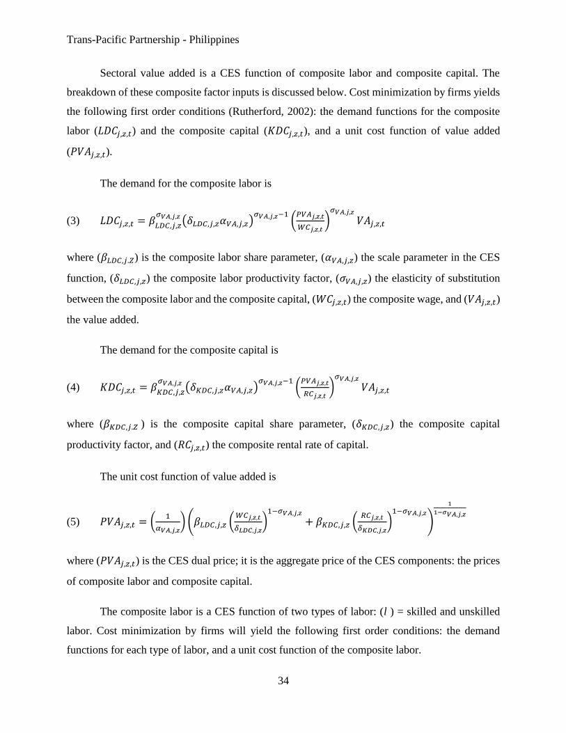
Sectoral value added is a CES function of composite labor and composite capital. The

breakdown of these composite factor inputs is discussed below. Cost minimization by firms yields

the following first order conditions (Rutherford, 2002): the demand functions for the composite

labor (𝐿𝐷𝐶𝑗,𝑧,𝑡) and the composite capital (𝐾𝐷𝐶𝑗,𝑧,𝑡), and a unit cost function of value added

(𝑃𝑉𝐴𝑗,𝑧,𝑡).

The demand for the composite labor is

(3) 𝐿𝐷𝐶𝑗,𝑧,𝑡 = 𝛽𝐿𝐷𝐶,𝑗,𝑧

𝜎𝑉𝐴,𝑗,𝑧 (𝛿𝐿𝐷𝐶,𝑗,𝑧𝛼𝑉𝐴,𝑗,𝑧)𝜎𝑉𝐴,𝑗,𝑧−1

(𝑃𝑉𝐴𝑗,𝑧,𝑡

𝑊𝐶𝑗,𝑧,𝑡)

𝜎𝑉𝐴,𝑗,𝑧

𝑉𝐴𝑗,𝑧,𝑡

where (𝛽𝐿𝐷𝐶,𝑗.𝑍) is the composite labor share parameter, (𝛼𝑉𝐴,𝑗,𝑧) the scale parameter in the CES

function, (𝛿𝐿𝐷𝐶,𝑗,𝑧) the composite labor productivity factor, (𝜎𝑉𝐴,𝑗,𝑧) the elasticity of substitution

between the composite labor and the composite capital, (𝑊𝐶𝑗,𝑧,𝑡) the composite wage, and (𝑉𝐴𝑗,𝑧,𝑡)

the value added.

The demand for the composite capital is

(4) 𝐾𝐷𝐶𝑗,𝑧,𝑡 = 𝛽𝐾𝐷𝐶,𝑗,𝑧

𝜎𝑉𝐴,𝑗,𝑧 (𝛿𝐾𝐷𝐶,𝑗,𝑧𝛼𝑉𝐴,𝑗,𝑧)𝜎𝑉𝐴,𝑗,𝑧−1

(𝑃𝑉𝐴𝑗,𝑧,𝑡

𝑅𝐶𝑗,𝑧,𝑡)

𝜎𝑉𝐴,𝑗,𝑧

𝑉𝐴𝑗,𝑧,𝑡

where (𝛽𝐾𝐷𝐶,𝑗.𝑍 ) is the composite capital share parameter, (𝛿𝐾𝐷𝐶,𝑗,𝑧) the composite capital

productivity factor, and (𝑅𝐶𝑗,𝑧,𝑡) the composite rental rate of capital.

The unit cost function of value added is

(5) 𝑃𝑉𝐴𝑗,𝑧,𝑡 = (1

𝛼𝑉𝐴,𝑗,𝑧) (𝛽𝐿𝐷𝐶,𝑗,𝑧 (

𝑊𝐶𝑗,𝑧,𝑡

𝛿𝐿𝐷𝐶,𝑗,𝑧)

1−𝜎𝑉𝐴,𝑗,𝑧

+ 𝛽𝐾𝐷𝐶,𝑗,𝑧 (𝑅𝐶𝑗,𝑧,𝑡

𝛿𝐾𝐷𝐶,𝑗,𝑧)


)

1


where (𝑃𝑉𝐴𝑗,𝑧,𝑡) is the CES dual price; it is the aggregate price of the CES components: the prices

of composite labor and composite capital.

The composite labor is a CES function of two types of labor: (l ) = skilled and unskilled

labor. Cost minimization by firms will yield the following first order conditions: the demand

functions for each type of labor, and a unit cost function of the composite labor.


35

The demand for type l labor is

(6) 𝐿𝐷𝑙,𝑗,𝑧,𝑡 = 𝛽𝑙,𝑗,𝑧

𝜎𝐿𝐷,𝑗,𝑧(𝛿𝑙,𝑗,𝑧𝛼𝐿𝐷,𝑗,𝑧)𝜎𝐿𝐷,𝑗,𝑧−1

(𝑊𝐶𝑗,𝑧,𝑡

𝑊𝑇𝐼𝑙,𝑗,𝑧,𝑡)

𝜎𝐿𝐷,𝑗,𝑧

𝐿𝐷𝐶𝑗,𝑧,𝑡

where (𝛽𝑙,𝑗.𝑍) is the share parameter of type l labor, (𝛿𝑙,𝑗,𝑧t) the productivity factor of type l labor,

(𝛼𝐿𝐷,𝑗,𝑧) the scale parameter in the CES function, (𝜎𝐿𝐷,𝑗,𝑧) the elasticity of substitution between the

two types of labor, and (𝑊𝑇𝐼𝑙,𝑗,𝑧,𝑡) the wage rate of type l labor including payroll tax.

The unit cost function of the composite labor is

(7) 𝑊𝐶𝑗,𝑧,𝑡 = (1

𝛼𝐿𝐷,𝑗,𝑧) ( ∑ 𝛽𝑙,𝑗,𝑧𝑙 (

𝑊𝑇𝐼𝑙,𝑗,𝑧,𝑡

𝛿𝑙,𝑗,𝑧)

1−𝜎𝐿𝐷,𝑗,𝑧

)

1

1−𝜎𝐿𝐷,𝑗,𝑧

This is a CES dual price.

The composite capital is a CES function of two types of capital: (k) = physical capital and

land (which includes natural resources). However, land is only used in agriculture and mining

while physical capital in all sectors.

The demand for type k capital is

(8) 𝐾𝐷𝑘,𝑗,𝑧,𝑡 = 𝛽𝑘,𝑗,𝑧

𝜎𝐾𝐷,𝑗,𝑧(𝛿𝑘,𝑗,𝑧𝛼𝐾𝐷,𝑗,𝑧)𝜎𝐾𝐷,𝑗,𝑧−1

(𝑅𝐶𝑗,𝑧,𝑡

𝑅𝑇𝐼𝑘,𝑗,𝑧,𝑡)

𝜎𝐾𝐷,𝑧

𝐾𝐷𝐶𝑗,𝑧,𝑡

where (𝛽𝑘,𝑗.𝑍) is the share parameter of type k capital, (𝛿𝑘,𝑗,𝑧t) the productivity factor of type k

capital, (𝛼𝐾𝐷,𝑗,𝑧) the scale parameter in the CES function, (𝜎𝐾𝐷,𝑗,𝑧) the elasticity of substitution

between the two types of capital, and (𝑅𝑇𝐼𝑘,𝑗,𝑧,𝑡) the rental rate of type k capital including factor

tax on capital.

The unit cost function of the composite capital is

(9) 𝑅𝐶𝑗,𝑧,𝑡 = (1

𝛼𝐾𝐷,𝑗,𝑧) ( ∑ 𝛽𝑘,𝑗,𝑧𝑘 (

𝑅𝑇𝐼𝑘,𝑗,𝑧,𝑡

𝛿𝑘,𝑗,𝑧)

1−𝜎𝐾𝐷,𝑗,𝑧

)

1

1−𝜎𝐾𝐷,𝑗,𝑧

This is a CES dual price.


36

Income and Savings

In each region there is a single household and a government. Household income (𝑌𝐻𝑧,𝑡) is

composed of labor (𝑌𝐻𝐿𝑧,𝑡) and capital income (𝑌𝐻𝐾𝑧,𝑡).

(10) 𝑌𝐻𝑧,𝑡 = 𝑌𝐻𝐿𝑧,𝑡 + 𝑌𝐻𝐾𝑧,𝑡

Labor income is the sum of labor earnings from the two types of labor, while capital income

is the sum of rentals paid for the two types of capital less depreciation. That is,

(11) 𝑌𝐻𝐿𝑧,𝑡 = ∑ 𝑊𝑙,𝑧,𝑡𝐿𝐷𝑙,𝑗,𝑧,𝑡𝑙,𝑗

(12) 𝑌𝐻𝐾𝑧,𝑡 = ∑ 𝑅𝑘,𝑗,𝑧,𝑡𝐾𝐷𝑘,𝑗,𝑧,𝑡𝑘,𝑗 − 𝐷𝑒𝑝𝑧,𝑡

where (𝑊𝑙,𝑧,𝑡) is the wage rate of type l labor before payroll tax, (𝑅𝑘,𝑗,𝑧,𝑡) the sectoral rental rate of

type k capital before rental tax, and (𝐷𝑒𝑝𝑧,𝑡) the amount of depreciation (capital consumption

allowance).

The household disposable income (𝑌𝐷𝐻𝑧,𝑡), the household consumption budget (𝐶𝑇𝐻𝑧,𝑡),

and the household savings (𝑆𝐻𝑧,𝑡 ) are

(13) 𝑌𝐷𝐻𝑧,𝑡 = 𝑌𝐻𝑧,𝑡 − 𝑇𝐷𝐻𝑧,𝑡

(14) 𝐶𝑇𝐻𝑧,𝑡 = 𝑌𝐷𝐻𝑧,𝑡 − 𝑆𝐻𝑧,𝑡

(15) 𝑆𝐻𝑧,𝑡 = 𝑃𝐼𝑋𝐶𝑂𝑁𝑧,𝑡𝜂

𝑠ℎ0𝑧,𝑡 + 𝑠ℎ1𝑧𝑌𝐷𝐻𝑧,𝑡

where (𝑇𝐷𝐻𝑧,𝑡) is the household income tax, (𝑃𝐼𝑋𝐶𝑂𝑁𝑧,𝑡) the consumer price index, (𝑠ℎ0𝑧,𝑡) the

intercept in the savings function in t, (𝑠ℎ1𝑧) the slope of the savings function, and (𝜂) the price-

elasticity of indexed transfers and parameters.

Government

The revenue of the government (𝑌𝐺𝑧,𝑡) comes from three sources: household income tax

(𝑇𝐷𝐻𝑧,𝑡), production-related taxes (𝑇𝑃𝑅𝑂𝐷𝑁𝑧,𝑡), and products and imports taxes (𝑇𝑃𝑅𝐶𝑇𝑧,𝑡).


37

(16) 𝑌𝐺𝑧,𝑡 = 𝑇𝐷𝐻𝑧,𝑡 + 𝑇𝑃𝑅𝑂𝐷𝑁𝑧,𝑡 + 𝑇𝑃𝑅𝐶𝑇𝑧,𝑡

Income taxes paid by households are a linear function of total income, i.e.,

(17) 𝑇𝐷𝐻𝑧,𝑡 = 𝑃𝐼𝑋𝐶𝑂𝑁𝑧,𝑡𝜂

𝑡𝑡𝑑ℎ0𝑧,𝑡 + 𝑡𝑡𝑑ℎ0𝑧,𝑡𝑌𝐻𝑧,𝑡

The production-related taxes are: the taxes on payroll (𝑇𝐼𝑊𝑇𝑧,𝑡), the taxes on the use capital

(𝑇𝐼𝐾𝑇𝑧,𝑡), and the taxes on production (𝑇𝐼𝑃𝑇𝑧,𝑡).

(18) 𝑇𝑃𝑅𝑂𝐷𝑁𝑧,𝑡 = 𝑇𝐼𝑊𝑇𝑧,𝑡 + 𝑇𝐼𝐾𝑇𝑧,𝑡 + 𝑇𝐼𝑃𝑇𝑧,𝑡

The tax on payroll is

(19) 𝑇𝐼𝑊𝑇𝑧,𝑡 = ∑ 𝑇𝐼𝑊𝑙,𝑗,𝑧,𝑡𝑙,𝑗 = ∑ 𝑡𝑡𝑖𝑤𝑙,𝑗,𝑧,𝑡𝑊𝑙,𝑧,𝑡𝐿𝐷𝑙,𝑗,𝑧,𝑡𝑙,𝑗

where (𝑇𝐼𝑊𝑙,𝑗,𝑧,𝑡) is the revenue from payroll tax on type l labor, and (𝑡𝑡𝑖𝑤𝑙,𝑗,𝑧,𝑡) the rate of payroll

tax.

Similarly, the tax on the use of capital is

(20) 𝑇𝐼𝐾𝑇𝑧,𝑡 = ∑ 𝑇𝐼𝐾𝑘,𝑗,𝑧,𝑡𝑘,𝑗 = ∑ 𝑡𝑡𝑖𝑘𝑘,𝑗,𝑧,𝑡𝑅𝑘,𝑗,𝑧,𝑡𝐾𝐷𝑘,𝑗,𝑧,𝑡𝑘,𝑗

where (𝑇𝐼𝐾𝑘,𝑗,𝑧,𝑡) is the revenue from the tax on the use of type k capital, and (𝑡𝑡𝑖𝑘𝑘,𝑗,𝑧,𝑡) the tax

rate on the use of capital.

The production tax is

(21) 𝑇𝐼𝑃𝑇𝑧,𝑡 = ∑ 𝑇𝐼𝑃𝑗,𝑧,𝑡𝑗 = ∑ 𝑡𝑡𝑖𝑝𝑗,𝑧,𝑡𝑃𝑃𝑗,𝑧,𝑡𝑋𝑆𝑗,𝑧,𝑡𝑗

where (𝑇𝐼𝑃𝑗,𝑧,𝑡) is the revenue from the tax on production, (𝑡𝑡𝑖𝑃𝑗,𝑧,𝑡) the tax rate on the use of

capital, and (𝑃𝑃𝑗,𝑧,𝑡) the unit cost of sector j.

The taxes on products and imports are: the indirect taxes on commodities (𝑇𝐼𝐶𝑇𝑧,𝑡), the

duties levied on imports (𝑇𝐼𝑀𝑇𝑧,𝑡), and the export taxes (𝑇𝐼𝑋𝑇𝑧,𝑡).

(22) 𝑇𝑃𝑅𝐶𝑇𝑆𝑧,𝑡 = 𝑇𝐼𝐶𝑇𝑧,𝑡 + 𝑇𝐼𝑀𝑇𝑧,𝑡 + 𝑇𝐼𝑋𝑇𝑧,𝑡


38

The indirect tax on commodities is

(23) 𝑇𝐼𝐶𝑇𝑧,𝑡 = ∑ 𝑇𝐼𝐶𝑖,𝑧,𝑡𝑖

where (𝑇𝐼𝐶𝑖,𝑧,𝑡) is the revenue from indirect tax. Since commodities available in the domestic

market are composed of domestically produced goods and imports, (𝑇𝐼𝐶𝑖,𝑧,𝑡) has two components:

(𝑇𝐼𝐶𝑛𝑚,𝑧,𝑡) the indirect tax on non-imported commodities, and (𝑇𝐼𝐶𝑚,𝑧,𝑡) the indirect tax on

imported commodities.

The indirect tax on non-imported commodities is

(24) 𝑇𝐼𝐶𝑛𝑚,𝑧,𝑡 = 𝑡𝑡𝑖𝑐𝑛𝑚,𝑧,𝑡𝑃𝐿𝑛𝑚,𝑧,𝑡𝐷𝐷𝑛𝑚,𝑧,𝑡

where (𝑡𝑡𝑖𝑐𝑛𝑚,𝑧,𝑡) is the indirect tax rate on non-imported commodities, (𝑃𝐿𝑛𝑚,𝑧,𝑡) the price of

locally produced commodities excluding taxes, and (𝐷𝐷𝑛𝑚,𝑧,𝑡) the domestic demand for

commodity nm.

Import duties are levied on commodities that enter the border. When these commodities

are moved beyond the border into the various domestic markets, similar to the domestically

produced goods, they are charged with indirect taxes as well. Moreover, the border price of imports

includes trade margins. Taking all these factors together, the indirect tax on imported commodities

(𝑇𝐼𝐶𝑚,𝑧,𝑡) is

(25) 𝑇𝐼𝐶𝑚,𝑧,𝑡 = 𝑡𝑡𝑖𝑐𝑚,𝑧,𝑡{𝑃𝐿𝑚,𝑧,𝑡𝐷𝐷𝑚,𝑧,𝑡 ∑ [(1 + 𝑡𝑡𝑖𝑚𝑚,𝑧𝑗,𝑧,𝑡)(𝑃𝑊𝑀𝑚,𝑧𝑗,𝑧,𝑡 +𝑧𝑗

∑ 𝑃𝑊𝑀𝐺𝑖𝑗,𝑡𝑡𝑚𝑟𝑔𝑖𝑗,𝑚,𝑧𝑗,𝑧,𝑡𝑖𝑗 )𝑒𝑧,𝑡𝐼𝑀𝑚,𝑧𝑗,𝑧,𝑡]}

where (𝑡𝑡𝑖𝑐𝑚,𝑧,𝑡) the indirect tax rate on imports, (𝑡𝑡𝑖𝑚𝑚,𝑧𝑗,𝑧,𝑡) the rate of import duties,

(𝑃𝑊𝑀𝑚,𝑧𝑗,𝑧,𝑡) the world price of m imported from country/region zj by country/region z in

international currency, (𝑃𝑊𝑀𝐺𝑖𝑗,𝑡) the world price of trade margins in international currency,

(𝑡𝑚𝑟𝑔𝑖𝑗,𝑚,𝑧𝑗,𝑧,𝑡) the rate of international transport margin services, (𝑒𝑧,𝑡) the exchange rate, and

(𝐼𝑀𝑚,𝑧𝑗,𝑧,𝑡) imports.

The total government revenue (𝑇𝐼𝑀𝑇𝑧,𝑡) from duties on imports is given as


39

(26) 𝑇𝐼𝑀𝑇𝑧,𝑡 = ∑ 𝑇𝐼𝑀𝑚,𝑧𝑗,𝑧,𝑡𝑚,𝑧𝑗 = ∑ 𝑡𝑡𝑖𝑚𝑚,𝑧𝑗,𝑧,𝑡(𝑃𝑊𝑀𝑚,𝑧𝑗,𝑧,𝑡 +𝑚,𝑧𝑗

𝑃𝑊𝑀𝑚,𝑧𝑗,𝑧,𝑡)𝑒𝑧,𝑡𝐼𝑀𝑚,𝑧𝑗,𝑧,𝑡

The total government revenue (𝑇𝐼𝑋𝑇𝑧,𝑡) from export taxes is defined as

(27) 𝑇𝐼𝑋𝑇𝑧,𝑡 = ∑ 𝑇𝐼𝑋𝑥,𝑧,𝑧𝑗,𝑡𝑥,𝑧𝑗 = ∑ 𝑡𝑡𝑖𝑥𝑥,𝑧,𝑧𝑗,𝑡𝑃𝐸𝑥,𝑧,𝑧𝑗,𝑡𝐸𝑋𝑥,𝑧,𝑧𝑗,𝑡𝑥,𝑧𝑗

where (𝑇𝐼𝑋𝑥,𝑧,𝑧𝑗,𝑡) is the revenue from taxes on export by country/region z to country/region zj,

(𝑡𝑡𝑖𝑥𝑥,𝑧,𝑧𝑗,𝑡) the rate of export taxes, (𝑃𝐸𝑥,𝑧,𝑧𝑗,𝑡) the price of exports excluding export taxes, and

(𝐸𝑋𝑥,𝑧,𝑧𝑗,𝑡) exports.

Government savings (𝑆𝐺𝑧,𝑡) is total government revenue net of total current government

expenditure (𝐺𝑧,𝑡).

(28) 𝑆𝐺𝑧,𝑡 = 𝑌𝐺𝑧,𝑡 − 𝐺𝑧,𝑡

Domestic Demand

Household demand (𝐶𝑖,𝑧,𝑡) is derived by utility maximization subject to a budget constraint.

This process will yield the following consumption function11

(29) 𝐶𝑖,𝑧,𝑡𝑃𝐶𝑖,𝑧,𝑡 = 𝐶𝑖,𝑧,𝑡𝑀𝐼𝑁𝑃𝐶𝑖,𝑧,𝑡 + 𝛾𝑖,𝑧

𝐿𝐸𝑆(𝐶𝑇𝐻𝑧,𝑡 − ∑ 𝐶𝑖𝑗,𝑧,𝑡𝑀𝐼𝑁

𝑖𝑗 )

where (𝐶𝑖,𝑧,𝑡𝑀𝐼𝑁) is the minimum consumption of commodity, (𝑃𝐶𝑖,𝑧,𝑡) the purchaser price of

commodity, and (𝛾𝑖,𝑧𝐿𝐸𝑆) the marginal share of commodity in the household consumption budget.

The volume of government expenditure on commodities (𝐶𝐺𝑖,𝑧,𝑡) is given by

(30) 𝐶𝐺𝑖,𝑧,𝑡𝑃𝐶𝑖,𝑧,𝑡 = 𝛾𝑖,𝑧𝐺𝑉𝑇𝐺𝑧,𝑡

11 This is a linear expenditure system (LES).


40

where (𝛾𝑖,𝑧𝐺𝑉𝑇) is the share of expenditure on commodities in the total current government

expenditure. The total current government expenditure is equal to the total real government

expenditure (𝑅𝐺𝑧,𝑡) multiplied by a public (government) expenditure price index (𝑃𝐼𝑋𝐺𝑉𝑇𝑧,𝑡), i.e.,

(31) 𝐺𝑧,𝑡 = 𝑅𝐺𝑧,𝑡𝑃𝐼𝑋𝐺𝑉𝑇𝑧,𝑡

The public expenditure price index is defined later. The equation (31) allows for alternative model

closures in the sense that government expenditure can either be fixed in real or in nominal terms.

The total investment in each country/region is determined by the savings-investment

equilibrium constraint which is be defined later. The total available investment (𝐼𝑇𝑧,𝑡) is distributed

across sectors using a set of fixed shares

(32) 𝐼𝑁𝑉𝑖,𝑧,𝑡𝑃𝐶𝑖,𝑧,𝑡 = 𝛾𝑖,𝑧𝐼𝑁𝑉𝐼𝑇𝑧,𝑡

where (𝐼𝑁𝑉𝑖,𝑧,𝑡) is the final demand for commodity for investment purposes (or the gross fixed

capital formation), and (𝛾𝑖,𝑧𝐼𝑁𝑉) the share of commodity in the total investment expenditures12.

The total intermediate demand (𝐷𝐼𝑇𝑖,𝑧,𝑡) for each commodity is the sum of the industry

demands for production inputs (𝐷𝐼𝑖,𝑗,𝑧,𝑡), i.e.,

(33) 𝐷𝐼𝑇𝑖,𝑧,𝑡 = ∑ 𝐷𝐼𝑖,𝑗,𝑧,𝑡𝑗

Supplies and International Trade

The supply of produced output in each country/region is represented by two-level nested

CET functions: (a) in the first nest, each sectoral output produced (𝑋𝑆𝑗,𝑧,𝑡) is allocated to three

outlets: domestic demand (𝐷𝑆𝑗,𝑧,𝑡), exports (𝐸𝑋𝑇𝑗,𝑧,𝑡), and international transport margin services

(𝑀𝑅𝐺𝑁𝑗,𝑧,𝑡); and (b) in the second nest, the total export of each country/region is distributed to the

various export market destinations. However, not all output produced are exportable. Some goods

are only sold in the domestic market. Thus, the commodities are grouped in two sets: (x) for output

12As pointed out in Robichaud, et al (2011), this specification implies that the production of new capital is Cobb-

Douglas. Thus, the quantity demanded for each commodity for investment purposes under a given amount of

investment expenditure is inversely related to its price.


41

sold in both exports and the domestic markets, and (nx) for output sold in the domestic market

only.

Producers allocate output to the three outlets in order to maximize revenue given product

prices in each of the outlets. Assuming imperfect substitutability among the three outlets, the

product is supplied to each outlet based on a CET function. The first order conditions yield supply

of exports, domestic demand, and international transport margin services.

The supply of exports is

(34) 𝐸𝑋𝑇𝑥,𝑧,𝑡 = 𝛽𝑥,𝑧𝐸𝑋𝑇𝛼1𝑥,𝑧

−(1+𝜎1𝑥,𝑧)(

𝑃𝑥,𝑧,𝑡

𝑃𝐸𝑇𝑥,𝑧,𝑡)

−𝜎1𝑥,𝑧

𝑋𝑆𝑥,𝑧,𝑡

where (𝛽𝑥,𝑧𝐸𝑋𝑇) is the share parameter in the CET function for exports, (𝛼1𝑥,𝑧) the scale parameter

in the CET function in the first nest, (𝜎1𝑥,𝑧) the elasticity of transformation in the first nest, (𝑃𝑥,𝑧,𝑡)

the basic price of commodities, and (𝑃𝐸𝑇𝑥,𝑧,𝑡) the border price of exports excluding export taxes.

The supply of goods sold in the domestic market is

(35) 𝐷𝑆𝑥,𝑧,𝑡 = 𝛽𝑥,𝑧𝐷𝑆𝛼1𝑥,𝑧

−(1+𝜎1𝑥,𝑧)(

𝑃𝑥,𝑧,𝑡

𝑃𝐿𝑥,𝑧,𝑡)

−𝜎1𝑥,𝑧


where (𝛽𝑥,𝑧𝐷𝑆) is the share parameter in the CET function for domestic demand, and (𝑃𝐿𝑥,𝑧,𝑡) the

price of locally produced commodities excluding indirect taxes.

The supply of international transport margin services is

(36) 𝑀𝑅𝐺𝑁𝑥,𝑧,𝑡 = 𝛽𝑥,𝑧𝑀𝑅𝐺𝑁𝛼1𝑥,𝑧

−(1+𝜎1𝑥,𝑧)(

𝑃𝑥,𝑧,𝑡

𝑒𝑧,𝑡𝑃𝑊𝑀𝐺𝑥,𝑧,𝑡)

−𝜎1𝑥,𝑧


where (𝛽𝑥,𝑧𝑀𝑅𝐺𝑁) is the share parameter in the CET function for domestic demand, and (𝑃𝑊𝑀𝐺𝑥,𝑧,𝑡)

the world price of imports of international transport margin services in international currency.

The basic price is the CET dual price which is an aggregate price of the CET components.

It is given by


42

(37) 𝑃𝑥,𝑧,𝑡 = (1

𝛼1𝑥,𝑧) (𝛽𝑥,𝑧

𝐸𝑋𝑇(𝑃𝐸𝑇𝑥,𝑧,𝑡)1+𝜎1𝑥,𝑧

+ 𝛽𝑥,𝑧𝐷𝑆(𝑃𝐿𝑥,𝑧,𝑡)

1+𝜎1𝑥,𝑧+

𝛽𝑥,𝑧𝑀𝑅𝐺𝑁(𝑒𝑧,𝑡𝑃𝑊𝑁𝐺𝑥,𝑧,𝑡)

1+𝜎1𝑥,𝑧)

1

1+𝜎1𝑥,𝑧

The total exports of each country/region is disaggregated to the various export destinations

using a second nest CET function. The first order conditions for revenue maximization yield the

supply of exports of country/region z in export destination zj

(38) 𝐸𝑋𝑥,𝑧,𝑧𝑗,𝑡 = 𝛽𝑥,𝑧,𝑧𝑗𝛼2𝑥,𝑧−(1+𝜎2𝑥,𝑧)

(𝑃𝐸𝑇𝑥,𝑧,𝑡

𝑃𝐸𝑥,𝑧,𝑧𝑗,𝑡)

−𝜎2𝑥,𝑧

𝐸𝑋𝑇𝑥,𝑧,𝑡

where (𝛽𝑥,𝑧,𝑧𝑗) is the share parameter in the CET function, (𝛼2𝑥,𝑧) the scale parameter in the CET

function in the second nest, (𝜎2𝑥,𝑧) the elasticity of transformation in the second nest, and (𝑃𝐸𝑥,𝑧,𝑡)

the price of exports excluding export taxes.

The dual CET price is

(39) 𝑃𝐸𝑇𝑥,𝑧,𝑡 = (1

𝛼2𝑥,𝑧) (∑ 𝛽𝑥,𝑧,𝑧𝑗𝑧𝑗 𝑃𝐸𝑥,𝑧,𝑧𝑗,𝑡

1+𝜎2𝑥,𝑧 )

1

1+𝜎2𝑥,𝑧

For commodities which are not exported their output prices are

(40) 𝑃𝑛𝑥,𝑧,𝑡 = 𝑃𝐿𝑛𝑥,𝑧,𝑡

The supply of each commodity in the domestic market of each country/region is

represented by two-level nested CES function: (a) in the first level is an Armington composite

good consisting of domestically produced commodities and composite imports; and (2) in the

second level is a disaggregation of imports from various countries/regions of origin. Also, since

not all commodities have competing imports, commodities are grouped in two sets: (m) for

commodities with competing imports, and (nm) for commodities supplied by domestically

produced goods only.

The first order conditions for cost minimization will yield the demand for domestically

produced goods, and the demand for the composite imports, and a composite import price. The

demand for domestically produced goods (𝐷𝐷𝑚,𝑧,𝑡) is


43

(41) 𝐷𝐷𝑚,𝑧,𝑡 = 𝛽𝐷𝐷,𝑚,𝑧

𝜎1𝑚,𝑧 (𝛼1𝑚,𝑧)𝜎1𝑚,𝑧−1

(𝑃𝐶𝑚,𝑧,𝑡

𝑃𝐷𝑚,𝑧,𝑡)

𝜎1𝑚,𝑧

𝑄𝑚,𝑧,𝑡

where (𝛽𝐷𝐷,𝑚,𝑧) is the share parameter for domestically produced goods, (𝛼1𝑚,𝑧) the scale

parameter in the CES function in the first nest, (𝜎1𝑚,𝑧) the elasticity of substitution in the first

nest, (𝑃𝐶𝑚,𝑧,𝑡) the purchaser price of commodity, (𝑃𝐷𝑚,𝑧,𝑡) the price of locally produced goods

sold in the domestic market including taxes, and (𝑄𝑚,𝑧,𝑡) the Armington composite good.

The demand for the composite imports (𝐼𝑀𝑇𝑚,𝑧,𝑡) is given by

(42) 𝐼𝑀𝑇𝑚,𝑧,𝑡 = 𝛽𝐼𝑀𝑇,𝑚,𝑧


(𝑃𝐶𝑚,𝑧,𝑡

𝑃𝑀𝑇𝑚,𝑧,𝑡)

𝜎1𝑚,𝑧

𝑄𝑚,𝑧,𝑡

where (𝛽𝐼𝑀𝑇,𝑚,𝑧) is the share parameter for the composite imports, and (𝑃𝑀𝑇𝑚,𝑧,𝑡) the price of the

composite imports.

The CES dual price is the composite price of (𝑃𝐷𝑚,𝑧,𝑡) and (𝑃𝑀𝑇𝑚,𝑧,𝑡), i.e.,

(43) 𝑃𝐶𝑚,𝑧,𝑡 = (1

𝛼1𝑚,𝑧) (𝛽𝐷𝐷,𝑚,𝑧(𝑃𝐷𝑚,𝑧,𝑡)

1−𝜎1𝑚,𝑧+ 𝛽𝐼𝑀𝑇,𝑚,𝑧(𝑃𝑀𝑇𝑚,𝑧,𝑡)

1−𝜎1𝑚,𝑧)

1

1−𝜎1𝑚,𝑧

The total imports of each commodity in each country/region is disaggregated into imports

from various countries/regions of origin using a second CES nest. The first order conditions for

cost minimization yields the import demand for imports by z from zj

(44) 𝐼𝑀𝑚,𝑧𝑗,𝑧,𝑡 = 𝛽𝑚,𝑧𝑗,𝑧


(𝑃𝑀𝑇𝑚,𝑧,𝑡

𝑃𝑀𝑚,𝑧𝑗,𝑧,𝑡)

𝜎2𝑚,𝑧

𝐼𝑀𝑇𝑚,𝑧,𝑡

where (𝛽𝑚,𝑧𝑗,𝑧) is the share parameter for imports from origin zj, (𝜎2𝑚,𝑧) the elasticity of

substitution in the second nest, (𝛼2𝑚,𝑧) the scale parameter in the CES function in the second nest,

and (𝑃𝑀𝑚,𝑧𝑗,𝑧,𝑡) the price of imports inclusive of taxes, duties and trade margins.

The CES dual price is

(45) 𝑃𝑀𝑇𝑚,𝑧,𝑡 = (1

𝛼2𝑚,𝑧) (∑ 𝛽𝑚,𝑧𝑗,𝑧𝑧𝑗 (𝑃𝑀𝑚,𝑧𝑗,𝑧,𝑡)

1−𝜎2𝑚,𝑧)

1

1−𝜎2𝑚,𝑧


44

For commodities without competing imports their purchasing prices are given by

(46) 𝑃𝐶𝑛𝑚,𝑧,𝑡 = 𝑃𝐷𝑛𝑚,𝑧,𝑡

External Account

In the GTAP 8 database, information is available on the amount of trade margin in each

sector i associated with each bilateral trade flows between countries/regions z and zj. However,

there is no information available matching the producers of the international transport margin

services (𝑀𝑅𝐺𝑁𝑗,𝑧,𝑡) to the individual bilateral trade flows. Therefore, the disaggregating

international transport margin services similar to the breaking down of exports of goods and

services to the various export destination cannot be done because there are no information available

in the GTAP 8 database needed to calibrate this nest. Thus similar to the PEP-w-t- model, the

present model has the supply of 𝑀𝑅𝐺𝑁𝑥,𝑧,𝑡 in each country/region pooled in a sector called

‘external account’ (EA)’ and its production is shared among suppliers in each country/region

through a competitive process.

The EA receives payments (𝑌𝐸𝐴𝑧,𝑡) for the value imports of the country/region including

international transport margin services, i.e.,

(47) 𝑌𝐸𝐴𝑧,𝑡 = 𝑒𝑧,𝑡 ∑ {𝐼𝑀𝑚,𝑧𝑗,𝑡(𝑃𝑊𝑀𝑚,𝑧𝑗,𝑧,𝑡 + ∑ 𝑃𝑊𝑀𝐺𝑖,𝑡𝑡𝑚𝑟𝑔𝑖,𝑚,𝑧𝑗,𝑧𝑖 )}𝑚,𝑧𝑗

The saving in the EA (𝑆𝐸𝐴𝑧,𝑡) is the difference between total receipts and spending which

is given by

(48) 𝑆𝐸𝐴𝑧,𝑡 = 𝑌𝐸𝐴𝑧,𝑡 − 𝑒𝑧,𝑡 ∑ 𝑃𝑊𝑋𝑥,𝑧,𝑧𝑗,𝑡𝑥,𝑧𝑗 𝐸𝑋𝑥,𝑧,𝑧𝑗,𝑡 − 𝑒𝑧,𝑡 ∑ 𝑃𝑊𝑀𝐺𝑚,𝑡𝑚 𝑀𝑅𝐺𝑁𝑚,𝑧,𝑡

where (𝑃𝑊𝑋𝑥,𝑧,𝑧𝑗,𝑡) is the world price of x exported by country/region z to zj in international

currency.

The current account balance (𝐶𝐴𝐵𝑧,𝑡) of each country/region is the negative of (𝑆𝐸𝐴𝑧,𝑡),

i.e.,

(49) 𝐶𝐴𝐵𝑧,𝑡 = −𝑆𝐸𝐴𝑧,𝑡


45

Prices

The unit cost of a sector’s output (including taxes related to the use of capital and labor,

but excluding other production taxes) is given by

(50) 𝑃𝑃𝑗,𝑧,𝑡 =𝑃𝑉𝐴𝑗,𝑧,𝑡𝑉𝐴𝑗,𝑧,𝑡+𝑃𝐶𝐼𝑗,𝑧,𝑡𝐶𝐼𝑗,𝑧,𝑡

𝑋𝑆𝑗,𝑧,𝑡

where (𝑃𝐶𝐼𝑗,𝑧,𝑡) is the price of intermediate consumption which is given as

(51) 𝑃𝐶𝐼𝑗,𝑧,𝑡 =∑ 𝑃𝐶𝑖,𝑧,𝑡𝐷𝐼𝑖,𝑗,𝑧,𝑡𝑖

𝐶𝐼𝑗,𝑧,𝑡

There are various forms of taxes that appear in the model. The relationship between prices

before and after taxes are defined below. The basic price of production in (37) is the unit cost in

(50) plus production taxes, excluding taxes on the use of labor and capital which have already been

included in the unit cost. That is,

(52) 𝑃𝑗,𝑧,𝑡 = (1 + 𝑡𝑡𝑖𝑝𝑗,𝑧,𝑡)𝑃𝑃𝑗,𝑧,𝑡

where (𝑡𝑡𝑖𝑝𝑗,𝑧,𝑡) is the production tax rate.

The wage rate of type l labor including payroll tax in (6) and (7) is

(53) 𝑊𝑇𝐼𝑙,𝑗,𝑧,𝑡 = (1 + 𝑡𝑡𝑖𝑤𝑙,𝑗,𝑧,𝑡)𝑊𝑙,𝑧,𝑡

where (𝑡𝑡𝑖𝑤𝑙,𝑗,𝑧,𝑡) is the payroll tax rate, and (𝑊𝑙,𝑧,𝑡) is the wage rate of type l labor.

Similarly, the rental rate of type k capital including the rental tax rate on the use of capital

in (8) and (9) is

(54) 𝑅𝑇𝐼𝑘,𝑗,𝑧,𝑡 = (1 + 𝑡𝑡𝑖𝑘𝑘,𝑗,𝑧,𝑡)𝑅𝑘,𝑗,𝑧,𝑡

where (𝑡𝑡𝑖𝑘𝑘,𝑗,𝑧,𝑡) is the rental tax rate, and (𝑅𝑘,𝑗,𝑧,𝑡) is the rental rate of type k capital in sector j.

The price of locally produced commodities in (41) and (46) is


46

(55) 𝑃𝐷𝑖,𝑧,𝑡 = (1 + 𝑡𝑡𝑖𝑐𝑖,𝑧,𝑡)𝑃𝐿𝑖,𝑧,𝑡

where (𝑡𝑡𝑖𝑐𝑖,𝑧,𝑡) is the indirect tax rate.

The relationship between the export price and the world price of exports is

(56) 𝑃𝐸𝑥,𝑧,𝑧𝑗,𝑡(1 + 𝑡𝑡𝑖𝑥𝑥,𝑧,𝑧𝑗,𝑡) = 𝑒𝑧,𝑡𝑃𝑊𝑋𝑥,𝑧,𝑧𝑗,𝑡

where (𝑡𝑡𝑖𝑥𝑥,𝑧,𝑧𝑗,𝑡) is the export tax rate, and (𝑃𝑊𝑋𝑥,𝑧,𝑧𝑗,𝑡) is the world price of exports in

international currency.

The local price of imports is

(57) 𝑃𝑀𝑚,𝑧𝑗,𝑧,𝑡 = 𝑒𝑧,𝑡(1 + 𝑡𝑡𝑖𝑐𝑚,𝑧,𝑡)(𝑃𝑊𝑀𝑚,𝑧𝑗,𝑡 + ∑ 𝑃𝑊𝑀𝐺𝑖,𝑟𝑡𝑚𝑟𝑔𝑖,𝑚,𝑧𝑗,𝑧𝑖 )(1 +

𝑡𝑡𝑖𝑚𝑚,𝑧𝑗,𝑧,𝑡)

where (𝑃𝑊𝑀𝑚,𝑧𝑗,𝑡) is the world price of imports, and (𝑡𝑡𝑖𝑚𝑚,𝑧𝑗,𝑧,𝑡) is the import tariff rate.

The world price of exports and imports are the same

(58) 𝑃𝑊𝑋𝑥,𝑧,𝑧𝑗,𝑡 = 𝑃𝑊𝑀𝑚,𝑧,𝑧𝑗,𝑡 ∀ 𝑥 = 𝑚

The consumer price index is a Laspeyres index defined as

(59) 𝑃𝐼𝑋𝐶𝑂𝑁𝑧,𝑡 =∑ 𝑃𝐶𝑖,𝑧,𝑡𝐶𝑖,𝑧

0𝑖

∑ 𝑃𝐶𝑖𝑗,𝑧0 𝐶𝑖𝑗,𝑧

0𝑖𝑗

where (𝐶𝑖,𝑧0 ) is household demand at the base value, and (𝑃𝐶𝑖𝑗,𝑧

0 ) is consumer price at the base

value.

The investment price index is

(60) 𝑃𝐼𝑋𝐼𝑁𝑉𝑧,𝑡 = ∏ (𝑃𝐶𝑖,𝑧,𝑡

𝑃𝐶𝑖𝑗,𝑧0 )

𝛾𝑖,𝑧𝐼𝑁𝑉

𝑖

This price index is the dual price of a Cobb-Douglas function which describes the commodity

demand for investment purposes in (32).


47

Similarly, the public expenditure price index is

(61) 𝑃𝐼𝑋𝐺𝑉𝑇𝑧,𝑡 = ∏ (𝑃𝐶𝑖,𝑧,𝑡

𝑃𝐶𝑖𝑗,𝑧0 )

𝛾𝑖,𝑧𝐺𝑉𝑇

𝑖

which is also a dual price of a Cobb-Douglas function which describes the commodity demand for

public consumption in (31).

The GDP price deflator is a Fisher index defined as

(62) 𝑃𝐼𝑋𝐺𝐷𝑃𝑧,𝑡 = √∑ (𝑃𝑉𝐴𝑗,𝑧,𝑡)𝑗 (𝑉𝐴𝑗,𝑧

0 ) ∑ (𝑃𝑉𝐴𝑗,𝑧,𝑡)𝑗 (𝑉𝐴𝑗,𝑧,𝑡)

∑ (𝑃𝑉𝐴𝑗,𝑧0 )𝑗 (𝑉𝐴𝑗,𝑧

0 ) ∑ (𝑃𝑉𝐴𝑗,𝑧0 )𝑗 (𝑉𝐴𝑗,𝑧,𝑡)

Equilibrium

The equilibrium in the labor market is

(63) 𝐿𝑆𝑙,𝑧,𝑡 = ∑ 𝐿𝐷𝑙,𝑗,𝑧,𝑡𝑗

where (𝐿𝑆𝑙,𝑧,𝑡) is the supply of type l labor. This will determine the value of the wage rate (𝑊𝑙,𝑧,𝑡)

in (53).

The equilibrium in the capital market is

(64) 𝐾𝑆𝑘,𝑗,𝑧,𝑡 = ∑ 𝐾𝐷𝑘,𝑗,𝑧,𝑡𝑗

where (𝐾𝑆𝑙,𝑗,𝑧,𝑡) is the supply of type k capital in sector j. This will determine the value of the

sectoral rental rate of type k capital (𝑅𝑘,𝑗,𝑧,𝑡) in (54).

Total investment expenditure is equal total savings plus the amount of depreciation. Total

savings is the sum of household savings, government savings, and foreign savings (which is the

negative of the current account balance in (49)).

(65) 𝐼𝑇𝑧,𝑡 = 𝑆𝐻𝑧,𝑡 + 𝑆𝐺𝑧,𝑡 − 𝐶𝐴𝐵𝑧,𝑡 + 𝐷𝐸𝑃𝑧,𝑡


48

The amount of depreciation is the sum of capital consumption allowances for all types of

capital in all sectors, and the capital consumption allowance is a constant fraction of the

replacement value of capital, i.e.,

(66) 𝐷𝐸𝑃𝑧,𝑡 = 𝑃𝐾𝑧,𝑡 ∑ 𝛿𝑘,𝑗,𝑧𝐾𝑆𝑘,𝑗,𝑧,𝑡𝑘,𝑗

where (𝛿𝑘,𝑗,𝑧) is the depreciation rate of capital k in sector j, (𝐾𝑆𝑘,𝑗,𝑧,𝑡) is the sectoral supply of

type k capital, and (𝑃𝐾𝑧,𝑡) is the price of new capital which is defined later in the section on

dynamics.

The supply of commodity by local producers is equal to the domestic demand for that

commodity produced locally, i.e.,

(67) 𝐷𝑆𝑖,𝑧,𝑡 = 𝐷𝐷𝑖,𝑧,𝑡

The quantity of each commodity exported from z to zj is equal to the quantity imported

from z by zj, i.e.,

(68) 𝐸𝑋𝑥,𝑧,𝑧𝑗,𝑡 = 𝐼𝑀𝑚,𝑧,𝑧𝑗,𝑡 ∀ 𝑥 = 𝑚

The supply of international transport margin services is equal to the sum of the demand

associated with all bilateral (z,zj) trade flows in all ij commodities, i.e.,

(69) ∑ 𝑀𝑅𝐺𝑁𝑖,𝑧,𝑡 = ∑ 𝑡𝑚𝑟𝑔𝑖,𝑖𝑗,𝑧𝑗,𝑧𝐼𝑀𝑖𝑗,𝑧𝑗,𝑧,𝑡𝑧,𝑧𝑗,𝑖𝑗𝑧

Note that because of (47), (48), (58), (68) and (69), the sum of 𝑆𝑅𝑂𝑊𝑧,𝑡 expressed in

common international currency across countries/regions is zero.

The product market equilibrium where supply is equal to demand for each commodity in

the domestic market of each country/region is defined as

(70) 𝑄𝑖−1,𝑧,𝑡 = 𝐶𝑖−1,𝑧,𝑡 + 𝐶𝐺𝑖−1,𝑧,𝑡 + 𝐼𝑁𝑉𝑖−1,𝑧,𝑡 + 𝐷𝐼𝑇𝑖−1,𝑧,𝑡

Note that because of Walras Law, one of the demand-supply product equilibrium

conditions is redundant. Thus, (70) is over (i-1) only.


49

Gross Domestic Product

The gross domestic product at basic prices (𝐺𝐷𝑃𝑧,𝑡𝐵𝑃) of each country/region is defined as

the payments to factors plus taxes on production but excluding taxes on factors, i.e.,

(71) 𝐺𝐷𝑃𝑧,𝑡𝐵𝑃 = ∑ 𝑃𝑉𝐴𝑗,𝑧,𝑡𝑉𝐴𝑗,𝑧,𝑡 + 𝑇𝐼𝑃𝑇𝑧,𝑡𝑗

GDP at market price (𝐺𝐷𝑃𝑧,𝑡𝑀𝑃) is GDP at basic prices plus taxes on products and imports,

i.e.,

(72) 𝐺𝐷𝑃𝑧,𝑡𝑀𝑃 = 𝐺𝐷𝑃𝑧,𝑡

𝐵𝑃 + 𝑇𝑃𝑅𝐶𝑇𝑆𝑧,𝑡

Model Closure

The present global CGE model adopts the PEP-w-t model closure with the following

features:

(a) The numeraire is the GDP deflator of the reference country/region (𝑃𝐼𝑋𝐺𝐷𝑃𝑧𝑟,𝑡), where zr

is the reference country/region. In the present case, zr = Europe Union 25. In the PEP-w-t

model zr = United States.

(b) Government expenditure in real terms (𝑅𝐺𝑧,𝑡) in (31) is fixed in each period t in each

country/region.

(c) Public capital investment (𝐼𝑁𝐷𝑘=𝑐𝑎𝑝𝑖𝑡𝑎𝑙,𝑗=𝑔𝑜𝑣𝑟𝑛𝑚𝑒𝑛𝑡,𝑧,𝑡) is fixed in each period t in each

country/region.

(d) The supply of type l labor (𝐿𝑆𝑙,𝑧,𝑡) in (63) is fixed in each period t in each country/region.

This is however updated in the succeeding periods using the growth projections of the labor

force.

(e) The supply of type k capital in each sector (𝐾𝑆𝑘,𝑗,𝑧,𝑡) in (64) is fixed in each period t in each

country/region. This is however updated in the succeeding periods using a dynamic

equation discussed in the next section.


50

(f) The minimum consumption (𝐶𝑖,𝑧,𝑡𝑀𝐼𝑁) in (29) is fixed in each period t in each country/region.

(g) The exchange rate (𝑒𝑧,𝑡) is fixed in each in each period t in each country/region.

The model has been tested for homogeneity wherein changing the value of the numeraire

changes all price variables and the nominal values of the variables by the same proportion as the

change in the numeraire, but retains the volume of the variables as they are not affected.

Dynamics

The supply of sectoral capital (k=capital) in each country/region in period t+1 is equal to

the stock in the preceding period, minus depreciation, and plus the volume of new capital

investment in the preceding period. That is,

(73) 𝐾𝑆𝑘,𝑗,𝑧,𝑡+1 = 𝐾𝑆𝑘,𝑗,𝑧,𝑡(1 − 𝛿𝑘,𝑗,𝑧) + 𝐼𝑁𝐷𝑘,𝑗,𝑧,𝑡

where (𝐼𝑁𝐷𝑘,𝑗,𝑧,𝑡) is the volume of new capital investment of the private sector. The new capital

investment of the government (for j=government) is fixed in model closure (c) above. There is no

change in the supply of land (k=land) over time.

The total capital investment is constrained by the total investment in (65), i.e.,

(74) 𝐼𝑇𝑧,𝑡 = 𝑃𝐾𝑧,𝑡 ∑ 𝐼𝑁𝐷𝑘,𝑗,𝑧,𝑡𝑘,𝑗

where the price of new capital (𝑃𝐾𝑧,𝑡) which is given by

(75) 𝑃𝐾𝑧,𝑡 = (1

𝐴𝑧𝐾) ∏ (

𝑃𝐶𝑖,𝑧,𝑡

𝛾𝑖,𝑧𝐼𝑁𝑉 )

𝛾𝑖,𝑧𝐼𝑁𝑉

𝑖

where (𝐴𝑧𝐾) is a scale parameter.

Following Jung and Thorbecke (2001) the sectoral capital investment of the private sector

(j=private) is patterned after the specification of the Tobin’s q. That is,

(76) 𝐼𝑁𝐷𝑘,𝑗,𝑧,𝑡 = ∅𝑘,𝑗,𝑧 (𝑅𝑘,𝑗,𝑧,𝑡

𝑈𝑘,𝑗,𝑧,𝑡)

𝜎𝑘,𝑗,𝑧𝐼𝑁𝐶

𝐾𝑆𝑘,𝑗,𝑧,𝑡


51

where (𝑈𝑘,𝑗,𝑧,𝑡) is user cost of type k capital in sector j, (𝜎𝑘,𝑗,𝑧𝐼𝑁𝐶 ) is the elasticity of investment

demand relative to Tobin’s q. The user cost of capita is given as

(77) 𝑈𝑘,𝑗,𝑧,𝑡 = 𝑃𝐾𝑧,𝑡(𝛿𝑘,𝑗,𝑧 + 𝐼𝑅𝑗,𝑧,𝑡)

where (𝐼𝑅𝑗,𝑧,𝑡) is the interest rate in z in period t. This interest rate is a rationing device that adjusts

so as to satisfy the investment constraint in (74).

Baseline Scenario

The standard reference scenario is called the ‘business as usual (BaU)’ scenario. This

scenario is generated using the individual countries/regions projections on population (from the

population projections of the United Nations) and on GDP per capita (from the GDP growth

projections of the World Bank). The growth of the per capita GDP (𝑔𝑟𝑧,𝑡

𝐺𝐷𝑃𝑝𝑐) is

(78) 𝑔𝑟𝑧,𝑡

𝐺𝐷𝑃𝑝𝑐 =𝑔𝑟𝑧,𝑡

𝐺𝐷𝑃+1

𝑔𝑟𝑧,𝑡𝑝𝑜𝑝

+1− 1

where (𝑔𝑟𝑧,𝑡𝐺𝐷𝑃) is the growth rate of GDP, and (𝑔𝑟𝑧,𝑡

𝑝𝑜𝑝) is the growth rate of the population.

Following the PEP-w-t model, some variables and parameters are updated using an index

that incorporates the growth projections of the population and GDP. This index is

(79) 𝑔𝑑𝑝𝑖𝑛𝑑𝑒𝑥𝑧,𝑡 = (1 + 𝑔𝑟𝑧,𝑡𝑝𝑜𝑝)(1 + 𝑔𝑟𝑧

𝐺𝐷𝑃̅̅ ̅̅ ̅̅ ̅̅ ̅)𝑔𝑑𝑝𝑖𝑛𝑑𝑒𝑥𝑧,𝑡−1, 𝑤𝑖𝑡ℎ 𝑔𝑑𝑝𝑖𝑛𝑑𝑒𝑥𝑧,𝑡=1 = 1

where ( 𝑔𝑟𝑧𝐺𝐷𝑃̅̅ ̅̅ ̅̅ ̅̅ ̅) is defined as

(80) 𝑔𝑟𝑧𝐺𝐷𝑃̅̅ ̅̅ ̅̅ ̅̅ ̅ = (

1

𝑇𝑇−𝑡=1) (∑ 𝑔𝑟𝑧,𝑡

𝐺𝐷𝑃𝑝𝑐𝑇𝑇−1𝑡=1 )

where t=1 is the first period and TT the last period. This index (𝑔𝑑𝑝𝑖𝑛𝑑𝑒𝑥𝑧,𝑡) is used to update the

following variables: 𝐶𝑖,𝑧,𝑡𝑀𝐼𝑁 in (29), 𝐿𝑆𝑙,𝑧,𝑡 in (63), 𝐼𝑁𝐷𝑘=𝑐𝑎𝑝𝑖𝑡𝑎𝑙,𝑗=𝑔𝑜𝑣𝑟𝑛𝑚𝑒𝑛𝑡,𝑧,𝑡 in item (c) of the

model closure, 𝑠ℎ0𝑧,𝑡 in (15), 𝑡𝑡𝑑ℎ0𝑧,𝑡 in (17), and 𝑅𝐺𝑧,𝑡 in (31).

Similar to PEP-w-t, the model can be solved so the value of the GDP of each country/region

align with the GDP projections of the World Bank. This is done by setting (𝑔𝑟𝑧,𝑡𝐺𝐷𝑃) equal to the


52

World Bank projections and solving for a multifactor productivity factor (𝐴𝑧,𝑡𝑉𝐴) for each

country/region over the simulation period (from t=1 to TT). The solution of the model using these

values of (𝐴𝑧,𝑡𝑉𝐴) will generate the GDP growth projections of the World Bank.

Elasticity of Substitution

(a) Between Domestic Products and Imports, and Among Imports of Origin

The elasticity of substitution between domestically produced commodities and imports (in

the first nest in the CES structure in (41), (42), and (43)) is

(81) 𝜎1𝑚,𝑧 = ∑ 𝑠ℎ𝑖,𝑚,𝑧𝑄

𝑖 𝐸𝑆𝑈𝐵𝐷𝑖

where (𝐸𝑆𝑈𝐵𝐷𝑖) is the elasticity parameter in the GTAP model, and (𝑠ℎ𝑖,𝑚,𝑧𝑄

) is share of sector i

in the base aggregate composite commodities (∑ 𝑄𝑚,𝑧0

𝑚 ) in each country/region. The value of the

elasticity of substitution among imports from the different trading partners (in the second nest in

the CES structure in (44) and (45)) is 𝜎2𝑚,𝑧 = 2 ∗ 𝜎1𝑚,𝑧.

(b) Between Factors of Production

The elasticity of substitution between the composite labor and composite capital (the first

nest in the CES structure in (3), (4), and (5)) is

(82) 𝜎𝑉𝐴,𝑗,𝑧 = ∑ 𝑠ℎ𝑗,𝑧𝑉𝐴

𝑗 𝐸𝑆𝑈𝐵𝑉𝐴𝑗

where (𝐸𝑆𝑈𝐵𝑉𝐴𝑖) is the elasticity parameter in the GTAP model, and (𝑠ℎ𝑗,𝑧𝑉𝐴) is share of sector j

in the base aggregate value added (∑ 𝑉𝐴𝑗,𝑧0

𝑗 ) in each country/region. The value of the elasticity of

substitution between the two types of labor (the second nest in the CES structure in (6) and (7)) is

𝜎𝐿𝐷,𝑗,𝑧 = 2 ∗ 𝜎𝑉𝐴,𝑗,𝑧. Similarly, the value of the elasticity of substitution between the two types of

capital (the second nest in the CES structure in (8) and (9)) is 𝜎𝐾𝐷,𝑗,𝑧 = 2 ∗ 𝜎𝑉𝐴,𝑗,𝑧.

(c) Between Domestic Market and Exports, and Among Export Destination


53

The elasticity of transformation in the first nest of the CET structure i(34), (35), and (36)

is 𝜎1𝑥,𝑧 = 2, while in the second nest in (38), and (39) is 𝜎2𝑥,𝑧 = 3.

Appendix B: Welfare Measure

The welfare measure used in the analysis is equivalent variation (EV). The global model

used in the analysis utilizes a LES system whose demand functions are given in (29). Robichaud

(2001) has shown that the EV corresponding to a demand system which is LES may be written as

(83) 𝐸𝑉𝑧,𝑡 = ∏ (𝑃𝐶𝑖,𝑧,𝑡

𝐵

𝑃𝐶𝑖,𝑧,𝑡𝑆 )

𝑔𝑎𝑚𝑚𝑎_𝐿𝐸𝑆𝑖,𝑧

(𝐶𝑇𝐻𝑧,𝑡𝑆 − ∑ 𝐶𝑀𝐼𝑁𝑖,𝑧,𝑡

𝐵𝑖 𝑃𝐶𝑖,𝑧,𝑡

𝑆 )𝑖 − (𝐶𝑇𝐻𝑧,𝑡𝐵 −

∑ 𝐶𝑀𝐼𝑁𝑖,𝑧,𝑡𝐵

𝑖 𝑃𝐶𝑖,𝑧,𝑡𝐵 )

where the superscript B refers to the baseline solution, while S to the simulation solution.

Documents

Potential Economic Effects on the Philippines of the Trans … · Potential Economic Effects on the Philippines of the Trans-Pacific Partnership (TPP)* Caesar B. Cororaton and David