Potential phytoplankton indicators for assessment of water

1

WATERS Report no 2016:8 Deliverable 3.3-3, Appendix: Gulf of Bothnia

Potential phytoplankton indicators for assessment of water quality in the coastal Gulf of Bothnia

Agneta Andersson1,2*, Chatarina Karlsson2, Siv Huseby2

1 Dept of Ecology and Environmental Science, Umeå University, SE-901 87 Umeå, Sweden

2 Umeå Marine Sciences Centre, Umeå University, SE-905 71 Hörnefors, Sweden

*Corresponding author. E-mail: [email protected]

2

Abstract

With the aim to develop phytoplankton indicators for assessment of coastal waters in the Gulf of Bothnia, we analysed a dataset collected in 25 basins. They were sampled 3-6 times during July-August 2011. A total of 120 samplings were performed at 114 stations, and the sampling sites were in most cases randomly selected in the different basins. Seawater samples were collected in the upper mixed water layer, and phytoplankton and potential explanatory physicochemical were analysed. We hypothesized that high phosphorus, which is the growth limiting substance in the study area, cause an increase of the total phytoplankton biomass, but also that certain taxonomic groups and species would selectively be promoted, e.g. Oscillatoriales, Nostocales, Chlorophyceans, Planktothrix sp. and Aphanizomenon sp.. We furthermore expected that phosphorus would promote relatively large phytoplankton and affect the phytoplankton diversity (number of dominating taxa). The relation between the potential phytoplankton indicators and environmental factors (Tot N, Tot P, temperature and salinity) were tested using partial least square (PLS) analysis and linear regression.

Twelve different phytoplankton variables showed a significant relation to salinity, nine to Tot P, four to Tot N, and three to temperature. Phytoplankton abundance and average cell size did not show any significant relation to the tested environmental factors, while the diversity, tested as the number of taxa having a biomass >10% of the total phytoplankton biomass, showed a positive relation to salinity. As anticipated, many phytoplankton variables related positively to high concentrations of total phosphorus; total phytoplankton carbon biomass, biovolume and chlorophyll a concentrations, the orders Oscillatoriales, Nostocales and Chroococcales, the class Chrysophyceae and the genus Pseudanabaena spp. We conclude that these phytoplankton variables are all promising candidates for being indicators of coastal water quality in the Gulf of Bothnia, as they were found to be selectively promoted by high phosphorus concentrations, i.e. the growth limiting substance in the study area.

Key words: Coastal Gulf of Bothnia, Baltic Sea, Phytoplankton indicators, Total phytoplankton biomass, Cyanobacteria, Total phosphorus

3

Introduction

Phytoplankton is one of the biological variables considered to be suitable for ecological classification of coastal waters in Europe (European Water Framework Directive (WFD)). So far only chlorophyll a and total biovolume concentrations of phytoplankton are used for classifying Swedish coastal waters (Swedish Environmental Protection Agency 2007). It is well-known that total phytoplankton biomass respond positively to increased nutrient load/availability concentrations (e.g. Samuelsson and Andersson 2002). Due to this fact, chlorophyll a and total biovolume concentrations are the most commonly phytoplankton variables used in different assessment systems around Europe (Höglander et al. 2013). However, to be fully compliant with the WFD, also other potential indicators e.g. taxonomic composition, diversity, size-structure and specific problematic species should be tested and eventually included in the assessment system.

The overall purpose of this study was to develop phytoplankton indicators to be used for ecological classification of coastal waters. Specific aims were to test if specific phytoplankton classes, orders or species are suitable as indictors for nutrient load/availability, or if size structure and diversity can be used as indicator.

It is known from previous studies in the Baltic Sea that for example the problematic Oscillatorian species Planktothrix agardhii and the cyanophycean order Nostocales respond positively to increased nutrient load (Carstensen and Heiskanen 2007, Andersson et al. 2015). In this study we thus expected to find a similar pattern. The size structure would be related to the nutrient availability, in that low nutrient concentrations would promote small phytoplankton and high nutrient concentrations would promote growth of large phytoplankton (Legendre and Rassoulzadegan 1995, Samuelsson and Andersson 2002). We thus expected to find a positive relation between average cell-size and nutrient concentration. The diversity often shows a hump-shaped relation to productivity in the system (Cermeno et al. 2013), highest diversity is shown at intermediate nutrient levels while at high nutrient concentrations a few species “take over” and become dominant. The diversity would decrease. We thus expected a negative relationship between nutrient concentrations and number of dominating species.

Our study area was the coastal Gulf of Bothnia, which is mainly limited by phosphorus (Andersson et al. 1996). The Tot P concentrations varied with a factor of 10, indicating that we had reasonable phytoplankton gradient to examine. Tot N and Tot P were in this study used as proxy for the carrying capacity of the system. Assuming a significant turnover of N and P in the system, the Tot N and Tot P concentrations would reflect nutrients available to the planktonic organisms. The data set used in this study has not earlier been used for development of phytoplankton indicators.

Material and Methods

The study comprised 120 samplings at 114 different stations in the coastal Gulf of Bothnia during July-August 2011 (Table 1, Fig. 1-3). Temperature and salinity were measured using CTD probes (SeaBird, USA). Samples for phytoplankton and chlorophyll a were sampled using a 0 to 10 m plastic hose. If depths were lower than 10 m, samples were taken from surface down to maximum depth minus 1 m with the hose (Table 1). The phytoplankton samples were then preserved with acidic Lugol´s

4

solution and analyzed using the Utermöhl technique (HELCOM 2014) and biomass was calculated according to Menden-Deuer and Lessard (2000). For chlorophyll a 100 mL of the samples were filtered and measured by spectroflourometer spectrophotometer at 680 nm (HELCOM 2003). Samples for total nitrogen (Tot N) and total phosphorus (Tot P) were collected in surface water and at 5 and 10 m depth when that could be accomplished (Table 1). Tot N and Tot P samples from both areas were oxidized using a modified method of Koroleff (1983) and then analyzed by flow injection analysis and segmented continuous flow analysis (Traacs 800 system, Bran + Luebbe and Quattro system, Seal Analytical) (Grasshoff 1983, Helcom guidelines (HELCOM 2014). Average values were then calculated for the 3 depths. Statistical analyses Partial least square analysis was performed on the impact of the environmental factors salinity, temperature TotN and TotP on total phytoplankton carbon biomass, biovolume, chlorophyll a, and autotrophic + mixotrophic forms of the phytoplankton classes and orders: Charophyceae, Chlorophyceae, Chrysophyceae, Cryptophyceae, Bacillariales (pennate diatoms), Eupodiales (centric diatoms), Dinophyceae, Eugleophyceae, Litostomatea (Mesodinium rubrum), Flagellates, Oscillatoriales, Chroococcales, Nostocales, Prasinophyceae and Prymnesiophyceae. Furthermore the relation between the environmental factors and phytoplankton abundance (average number of phytoplankton units/l), unit size (average carbon biomass/unit) and “diversity” (number of taxa accounting for >10% of the total phytoplankton biomass) were tested. Finally, the relationship between the identified 20 dominant taxa and the environmental factors were tested. Log-transformed data were analysed using the program SIMCA 14. Each phytoplankton variable were tested separately in relation to the environmental factors. The data were cross validated to determine the number of significant components. Permutation analysis were performed to test the selected phytoplankton variables. Analysis of variance (ANOVA) was performed on the residuals in the cross validated phytoplankton variables and p-values indicate the significance of the investigated model. For those models having a p-value <0.05, regression coefficient plots were performed to identify and visualize “prediction vectors”, i.e. environmental factors affecting the tested phytoplankton variables. Factors with error bars not crossing the zero-line were identified as positive or negative drivers of the tested phytoplankton variable. Results Distribution of environmental factors in the studied coastal area The environmental factor Tot P showed the largest variation, varying with at factor of 11 in the coastal gradient (Table 2). Tot N varied with a factor of 4. The salinity spanned from 1-4.9 units and the temperature from 10 to 21°C. Relation between total phytoplankton carbon biomass, biovolume and chlorophyll a and environmental factors

5

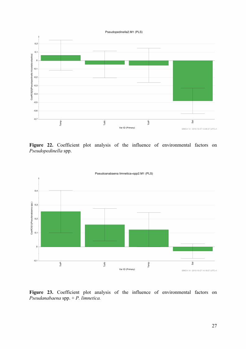
The total phytoplankton biomass, measured as carbon biomass, biovolume and chlorophyll a ranged a factor 20-40 in the studied coastal gradient (Table 2). PLS analysis showed that Tot P had a relatively strong positive influence on all these factors (Fig. 4-6, Table 3). Linear regression analysis also showed a positive relation between these phytoplankton variables and Tot P (Fig. 7). Relation between phytoplankton abundance, cell size and diversity and environmental factors The average cell size varied with a factor of ~700 in the coastal gradient and the abundance showed an even larger range, varying with a factor of ~16 000 (Table 2). Neither average cell size nor phytoplankton abundances showed any significant relation to the measured environmental factors (Table 3). The number of taxa accounting for >10% of the phytoplankton biomass (diversity), ranged from 1 to 6 (Table 3). The summed biomass of the dominant taxa ranged from 23-95% of the total phytoplankton biomass (Fig 8, Table 3). The diversity showed a positive relation to salinity (Fig 9). Relation between phytoplankton classes, orders, diversity and environmental factors Fifteen different phytoplankton classes and orders were investigated for potential relationship to environmental factors (Table 3). For eleven of them a significant PLS model was obtained (Table 3), and for eight of them driving environmental factors were identified (Table 3, Fig. 10-17). Flagellates, Dinophyceae and Nostocales were positively influenced by salinity (Table 3, Fig. 11, 12, 14), while Oscillatoriales, Nostocales Chroococcales and Chrysophyceae were promoted by Tot P (Table 3, Fig. 7, 10, 14, 15, 16). Dinophyceae was the only phytoplankton class containing heterotrophic forms. The proportion of heterotrophic Dinophyeae ranged from 0-100% at different stations, with an average of 44%. The relation between heterotrophic dinophyceans and environmental factors was not evaluated. Relation between dominating phytoplankton taxa and environmental factors Twenty phytoplankton taxa were found to have a biomass >10% of the total phytoplankton biomass (Table 3). For eight of them a significant PLS model was obtained (Table 3), and for nine of them driving environmental factors were identified (Table 3, Fig. 18-25). Aphanizomenon spp. And Dinophysis acuminata were found to have a positive relation to salinity (Fig. 18, 20), while Diatoma tenuis, Pseudopedinella spp. and Uroglena spp. were found to have a negative relation to salinity (Fig. 19, 22, 25). Pseudopedinella spp. was also found to have a positive relation to Tot P (Fig. 7, 23). Measurement of phytoplankton biomass

Total phytoplankton biomass were measured as carbon biomass, biovolume and chlorophyll a. Regression analysis showed strong relationships between all these variables (Fig. 26). For most of the phytoplankton, the carbon density was relatively similar (Fig. 27). A conversion factor of phytoplankton carbon biomass to wet-weight biomass of 157 µg C/mm3 (Fig. 27) was estimated.

6

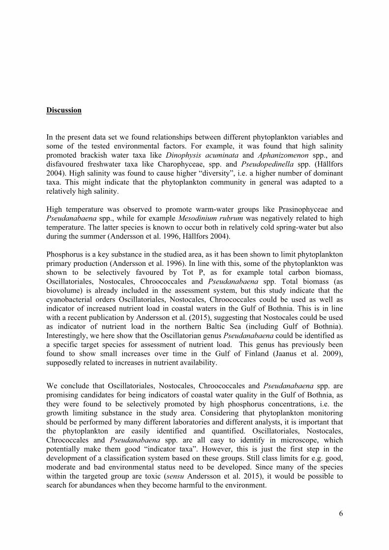
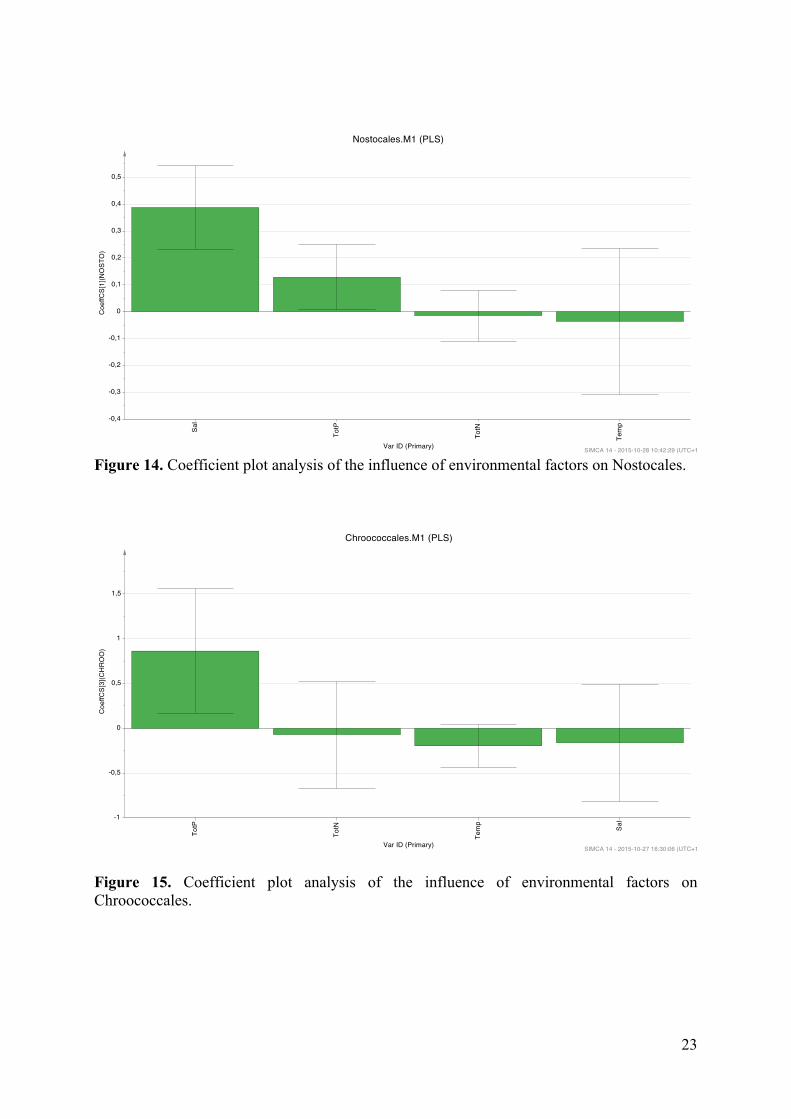
Discussion In the present data set we found relationships between different phytoplankton variables and some of the tested environmental factors. For example, it was found that high salinity promoted brackish water taxa like Dinophysis acuminata and Aphanizomenon spp., and disfavoured freshwater taxa like Charophyceae, spp. and Pseudopedinella spp. (Hällfors 2004). High salinity was found to cause higher “diversity”, i.e. a higher number of dominant taxa. This might indicate that the phytoplankton community in general was adapted to a relatively high salinity. High temperature was observed to promote warm-water groups like Prasinophyceae and Pseudanabaena spp., while for example Mesodinium rubrum was negatively related to high temperature. The latter species is known to occur both in relatively cold spring-water but also during the summer (Andersson et al. 1996, Hällfors 2004). Phosphorus is a key substance in the studied area, as it has been shown to limit phytoplankton primary production (Andersson et al. 1996). In line with this, some of the phytoplankton was shown to be selectively favoured by Tot P, as for example total carbon biomass, Oscillatoriales, Nostocales, Chroococcales and Pseudanabaena spp. Total biomass (as biovolume) is already included in the assessment system, but this study indicate that the cyanobacterial orders Oscillatoriales, Nostocales, Chroococcales could be used as well as indicator of increased nutrient load in coastal waters in the Gulf of Bothnia. This is in line with a recent publication by Andersson et al. (2015), suggesting that Nostocales could be used as indicator of nutrient load in the northern Baltic Sea (including Gulf of Bothnia). Interestingly, we here show that the Oscillatorian genus Pseudanabaena could be identified as a specific target species for assessment of nutrient load. This genus has previously been found to show small increases over time in the Gulf of Finland (Jaanus et al. 2009), supposedly related to increases in nutrient availability.

We conclude that Oscillatoriales, Nostocales, Chroococcales and Pseudanabaena spp. are promising candidates for being indicators of coastal water quality in the Gulf of Bothnia, as they were found to be selectively promoted by high phosphorus concentrations, i.e. the growth limiting substance in the study area. Considering that phytoplankton monitoring should be performed by many different laboratories and different analysts, it is important that the phytoplankton are easily identified and quantified. Oscillatoriales, Nostocales, Chrococcales and Pseudanabaena spp. are all easy to identify in microscope, which potentially make them good “indicator taxa”. However, this is just the first step in the development of a classification system based on these groups. Still class limits for e.g. good, moderate and bad environmental status need to be developed. Since many of the species within the targeted group are toxic (sensu Andersson et al. 2015), it would be possible to search for abundances when they become harmful to the environment.

7

Acknowledgement

This study was supported by grants from the research programmes WATERS and ECOCHANGE.

References

Andersson A, Hajdu S, Haecky P, Kuparinen J., Wikner, J. (1996) Succession and growth limitation of phytoplankton in the Gulf of Bothnia. Marine Biology. 126: 791-801

Andersson A, Höglander S, Karlsson C, Huseby S (2015) Key role of phosphorus and nitrogen in regulating cyanobacterial community composition in the northern Baltic Sea. Estuarine Coastal and Shelf Science 164: 161-171.

Carstensen J and Heiskanen A-S (2007) Phytoplankton responses to nutrient status: application of a screening method to the northern Baltic Sea. Marine Ecology Progress Series 336: 29-42.

Cermeno P, Rodriques-Ramos T, Dornelas M, Figueiras FG, Maranon E, Teixeira IG, Vallina

SM (2013) Species richness in marine phytoplankton communities is not correlated to ecosystem productivity. Mar. Ecol. Prog. Ser. 488: 1-9.

Grasshoff K, Ehrhardt M, Kremling K (1983) Methods of Seawater Analysis, 2nd edition,

Verlag Chemie, Weinheim, New York. Hällfors G (2004) Checklist of Baltic Sea phytoplankton species. Baltic Sea Environment

Proceedings No. 95. Helsinki Commission. Baltic Marine Environment Protection Commission.

HELCOM (1988) Guidelines for Baltic Monitoring Programme for the third stage. Part D.

Biological determinants. Baltic Sea Environment Proceedings No. 27 D. Höglander H, Karlson B, Johansen M, Walve J, Andersson A (2013) Overview of coastal

phytoplankton indicators and their potential use in Swedish waters. WATERS Report no. 2013:5

Jaanus A, Andersson A, Olenina I, Toming K, Kaljurand K (2011) Changes in phytoplankton

communities along a north-south gradient in the Baltic Sea between 1990 and 2008. Boreal Environment Research 16 (suppl A): 191-208.

Koroleff F (1983) Determination of nutrients, p. 125-139, 162-173. In: Grashoff K, Ehrhardt

M, Kremling K [Eds], Methods of seawater analysis. Verlag Chemie.

Legendre L and Rassoulzadegan F (1995) Plankton and nutrient dynamics in marine waters. Ophelia 41: 153-172.

Menden-Deuer S, Lessard EJ (2000) Carbon to volume relationsships for dinoflagellates, diatoms and other protist plankton. Limnol. Oceanogr. 45: 569-579.

8

Samuelsson K, Haecky P, Berglund J, Andersson A.(2002) Structural changes in an aquatic microbial food web caused by inorganic nutrient addition. Aquatic Microbial Ecology, 29:29-38.

Swedish Environmental Protection Agency (2007) Classification system for coastal waters and transitional waters. Handbook Appendix B.

Table 1. Sampling design in the northern Bothnian Sea.

Type Waterbody Station Sample date LATIT LONGI Maximum depth (m)

Sample depths (m) Chemistry

Sample depths

(m) Biology

18 Bäckfjärden SBa10 2011-08-01 6313,19 1842,15 38 1; 5; 10 10 18 Bäckfjärden SBa 2011-07-05 6314,32 1840,6 34 1; 5; 10 10 18 Bäckfjärden SBa6 2011-07-05 6313,89 1844,43 13 1; 5; 10 10 18 Bäckfjärden SBa7 2011-07-20 6313,74 1842,2 37 1; 5; 10 10 18 Bäckfjärden SBa8 2011-07-20 6314,7 1841,06 15 1; 5; 10 10 18 Bäckfjärden SBa9 2011-08-01 6314,33 1842,19 9 1; 4; 8 8 20 Djupsundsviken SDj3 2011-07-07 6341,22 2022,66 2 1; 1.5; 2 1 20 Djupsundsviken SDj4 2011-07-21 6341,16 2022,67 4 1; 2; 3 3 20 Djupsundsviken SDj5 2011-08-03 6341,25 2022,74 2 1; 1.5; 2 1 18 Dockstafjärden SDo10 2011-08-02 6301,99 1819,99 19 1; 5; 10 10 18 Dockstafjärden SDo5 2011-07-05 6301,96 1820,43 39 1; 5; 10 10 18 Dockstafjärden SDo6 2011-07-05 6302,8 1819,96 16 1; 5; 10 10 18 Dockstafjärden SDo7 2011-07-19 6301,94 1819,97 16 1; 5; 10 10 18 Dockstafjärden SDo8 2011-07-19 6303,1 1819,81 7 1; 4; 6 6 18 Dockstafjärden SDo9 2011-08-02 6301,74 1820,25 53 1; 5; 10 10 20 Djupviken SDv3 2011-07-06 6340,15 2015,74 2 1; 1.5; 2 1 20 Djupviken SDv4 2011-07-21 6340,18 2015,92 3 1; 2; 3 2 20 Djupviken SDv5 2011-08-04 6340,2 2015,86 3 1; 2; 3 2 20 Fjärdgrundsområdet SFj10 2011-08-03 6339,51 2020,39 11 1; 5; 10 10 20 Fjärdgrundsområdet SFj5 2011-07-06 6338,83 2021,03 18 1; 5; 10 10 20 Fjärdgrundsområdet SFj6 2011-07-06 6340,47 2019,74 15 1; 5; 10 10 20 Fjärdgrundsområdet SFj7 2011-07-21 6338,68 2023,27 17 1; 5; 10 10 20 Fjärdgrundsområdet SFj8 2011-07-21 6339,86 2021,66 18 1; 5; 10 10 20 Fjärdgrundsområdet SFj9 2011-08-03 6339,32 2022,48 14 1; 5; 10 10 19 Germundsöfjärden SGe10 2011-08-02 6249,61 1820,2 56 1; 5; 10 10 19 Germundsöfjärden SGe5 2011-07-05 6251,42 1818,84 35 1; 5; 10 10 19 Germundsöfjärden SGe6 2011-07-05 6250,14 1817,16 74 1; 5; 10 10 19 Germundsöfjärden SGe7 2011-07-19 6252,42 1819,84 5 1; 3; 4 4 19 Germundsöfjärden SGe8 2011-07-19 6250,3 1818,96 34 1; 5; 10 10 19 Germundsöfjärden SGe9 2011-08-02 6251,74 1818,26 2 1; 1.5; 2 1

9

20 Gumbodafjärden SGu1 2011-07-07 6412,44 2105,28 12 11 8 20 Gumbodafjärden SGu1 2011-07-21 6412,46 2105,25 9 8 8 20 Gumbodafjärden SGu1 2011-08-04 6412,47 2105,13 9 8 8 19 Höga Kustens kustvatten SHK10 2011-08-02 6304,6 1853,66 157 1; 5; 10 10 19 Höga Kustens kustvatten SHK5 2011-07-04 6227,99 1754,11 100 1; 5; 10 10 19 Höga Kustens kustvatten SHK6 2011-07-05 6300,66 1841,8 41 1; 5; 10 10 19 Höga Kustens kustvatten SHK7 2011-07-19 6240,18 1808,85 90 1; 5; 10 10 19 Höga Kustens kustvatten SHK8 2011-07-19 6241,79 1809,44 73 1; 5; 10 10 19 Höga Kustens kustvatten SHK9 2011-08-02 6259,58 1843,03 53 1; 5; 10 10 20 Hörneforsområdet SHo10 2011-08-02 6334,25 1957,25 21 1; 5; 10 10 20 Hörneforsområdet SHo5 2011-07-05 6332,77 1954,64 20 1; 5; 10 10 20 Hörneforsområdet SHo6 2011-07-05 6333,4 2000,9 30 1; 5; 10 10 20 Hörneforsområdet SHo7 2011-07-21 6335,81 1957,99 12 1; 5; 10 10 20 Hörneforsområdet SHo8 2011-07-21 6335,39 1959,11 19 1; 5; 10 10 20 Hörneforsområdet SHo9 2011-08-02 6333,39 1954,92 18 1; 5; 10 10 18 Idbyfjärden SId10 2011-08-01 6316,22 1851,93 12 1; 5; 10 10 18 Idbyfjärden SId5 2011-07-04 6316,12 1852,38 17 1; 5; 10 10 18 Idbyfjärden SId6 2011-07-04 6317,5 1851,99 3 1; 2; 3 2 18 Idbyfjärden SId7 2011-07-18 6315,87 1851,82 6 1; 3; 5 5 18 Idbyfjärden SId8 2011-07-18 6316,56 1852,16 8 1; 4; 7 7 18 Idbyfjärden SId9 2011-08-01 6316,91 1851,47 9 1; 4; 8 8 20 Lillfjärden SLi1 2011-07-07 6349,74 2029,7 1 1 1 20 Lillfjärden SLi1 2011-07-21 6349,74 2029,7 1 1 1 20 Lillfjärden SLi1 2011-08-03 6349,74 2029,7 1 1 1 20 Ljumviken SLj3 2011-07-07 6341,58 2021,96 2 1; 1.5; 2 1 20 Ljumviken SLj4 2011-07-21 6341,48 2022,08 2 1; 1.5; 2 1 20 Ljumviken SLj5 2011-08-03 6341,54 2022 2 1; 1.5; 2 1 20 Megrundsområdet SMe3 2011-07-07 6336,85 1955 2 1; 1.5; 2 1 20 Megrundsområdet SMe4 2011-07-20 6336,89 1955,4 2 1; 1.5; 2 1 20 Megrundsområdet SMe5 2011-08-04 6336,83 1955,34 2 1; 1.5; 2 1 18 Näskefjärden SNa10 2011-08-02 6309,21 1831,44 9 1; 4; 8 8 18 Näskefjärden SNa5 2011-07-05 6309,42 1831,64 12 1; 5; 10 10 18 Näskefjärden SNa6 2011-07-05 6307,9 1832,48 32 1; 5; 10 10 18 Näskefjärden SNa7 2011-07-20 6307,34 1832,08 16 1; 5; 10 10 18 Näskefjärden SNa8 2011-07-20 6307,47 1833,72 18 1; 5; 10 10 18 Näskefjärden SNa9 2011-08-02 6308,8 1832,15 17 1; 5; 10 10

19 Norra Bottenhavets kustvatten SNB10 2011-08-02 6323,88 1927,23 27 1; 5; 10 10






18 Norrfjärden SNf10 2011-08-02 6303,56 1824,65 10 1; 5; 9 9

10

18 Norrfjärden SNf5 2011-07-05 6302,19 1823,94 10 1; 4; 9 9 18 Norrfjärden SNf6 2011-07-05 6301,56 1826,22 52 1; 5; 10 10 18 Norrfjärden SNf7 2011-07-20 6302,65 1825,64 77 1; 5; 10 10 18 Norrfjärden SNf8 2011-07-20 6301,29 1826,57 64 1; 5; 10 10 18 Norrfjärden SNf9 2011-08-02 6302,51 1823,88 15 1; 5; 10 10 18 Norafjärden SNo10 2011-08-02 6250,24 1800,93 21 1; 5; 10 10 18 Norafjärden SNo5 2011-07-05 6249,29 1805,05 58 1; 5; 10 10 18 Norafjärden SNo6 2011-07-05 6248,85 1808,43 13 1; 5; 10 10 18 Norafjärden SNo7 2011-07-19 6250,26 1802,54 52 1; 5; 10 10 18 Norafjärden SNo8 2011-07-19 6250,01 1800,59 16 1; 5; 10 10 18 Norafjärden SNo9 2011-08-02 6248,82 1807,88 14 1; 5; 10 10 20 Österfjärden SOf1 2011-07-06 6342,13 2020,24 17 16 10 20 Österfjärden SOf1 2011-07-21 6342,13 2020,24 15 14 10 20 Österfjärden SOf1 2011-08-03 6342,13 2020,24 17 16 10 20 Österlångslädan SOl10 2011-08-03 6341,63 2023,83 4 1; 2.5;4 3 20 Österlångslädan SOl5 2011-07-07 6341,88 2023,94 2 1; 1.5; 2 1 20 Österlångslädan SOl6 2011-07-07 6341,16 2024,33 2 1; 1.5; 2 1 20 Österlångslädan SOl7 2011-07-22 6341,43 2024,36 4 1; 3; 4 3 20 Österlångslädan SOl8 2011-07-22 6341,38 2023,92 3 1; 2; 3 2 20 Österlångslädan SOl9 2011-08-03 6341,53 2024,26 3 1; 2; 3 2 20 Östra Sundet SOS3 2011-07-06 6339,86 2016,41 2 1; 1.5; 2 1 20 Östra Sundet SOS4 2011-07-21 6339,56 2016,34 7 1; 4; 7 6 20 Östra Sundet SOS5 2011-08-04 6339,81 2016,58 2 1; 1.5; 2 1 20 Patholmsviken SPa3 2011-07-07 6341,68 2021,47 5 1; 3; 5 4 20 Patholmsviken SPa4 2011-07-21 6341,61 2021,37 6 1; 3; 5 5 20 Patholmsviken SPa5 2011-08-03 6341,79 2021,48 4 1; 2.5; 4 3 19 Skaghamnsfjärden SSk10 2011-08-01 6312,88 1902 15 1; 5; 10 10 19 Skaghamnsfjärden SSk5 2011-07-04 6312,45 1903,24 10 1; 4; 9 9 19 Skaghamnsfjärden SSk6 2011-07-04 6312,58 1901,94 27 1; 5; 10 10 19 Skaghamnsfjärden SSk7 2011-07-18 6311,96 1902,6 30 1; 5; 10 10 19 Skaghamnsfjärden SSk8 2011-07-18 6312,63 1902,2 29 1; 5; 10 10 19 Skaghamnsfjärden SSk9 2011-08-01 6312,62 1901,98 24 1; 5; 10 10 19 Stubbsandsfjärden SSt10 2011-08-01 6312,92 1857,4 14 1; 5; 10 10 19 Stubbsandsfjärden SSt5 2011-07-04 6312,1 1857,67 25 1; 5; 10 10 19 Stubbsandsfjärden SSt6 2011-07-04 6312,79 1856,63 19 1; 5; 10 10 19 Stubbsandsfjärden SSt7 2011-07-18 6312,36 1857,98 29 1; 5; 10 10 19 Stubbsandsfjärden SSt8 2011-07-18 6313,1 1857,39 14 1; 5; 10 10 19 Stubbsandsfjärden SSt9 2011-08-01 6312,67 1856,02 18 1; 5; 10 10 19 SannaUltrafjärden SSU10 2011-08-01 6316,4 1907,31 23 1; 5; 10 10 19 SannaUltrafjärden SSU5 2011-07-04 6316,35 1908,15 25 1; 5; 10 10 19 SannaUltrafjärden SSU6 2011-07-04 6315,93 1906,42 10 1; 4; 9 9 19 SannaUltrafjärden SSU7 2011-07-18 6315,93 1909,65 12 1; 5; 10 10 19 SannaUltrafjärden SSU8 2011-07-18 6316,11 1906,94 23 1; 5; 10 10 19 SannaUltrafjärden SSU9 2011-08-01 6316,94 1908,09 7 1; 3; 7 6 20 VästraSundet SVS3 2011-07-06 6339,69 2015,62 3 1; 2; 3 2 20 VästraSundet SVS4 2011-07-21 6339,71 2015,86 3 1; 2; 3 2

11

20 VästraSundet SVS5 2011-08-04 6339,71 2015,86 2 1; 1.5; 2 1

Table 2. Descriptive statistics for physicochemical and phytoplankton variables in the studied area in Gulf of Bothnia. Range factor is the ratio between the maximum and minimum observation.

Variable Range (min-max)

Range factor

Median Mean Stdev

Tot P (umol/l) 0.17-1.84 11 0.34 0.41 0.22

Tot N (umol/l) 14.8-56.0 4 16.9 18.8 6.0

Temperature (oC) 10.2-21.3 2 16.5 16.7 2.5

Salinity 1.0-4.9 5 4.0 3.7 1.0

Chla (ug/l) 1.2-13.4 23 2.37 2.94 1.94

Carbon biomass (ug/l)

10.3-370.6 36 48.6 61.7 57.0

Biovolume (mm3/l) 0.07-2.1 30 0.37 0.43 0.36

Carbon biomass /unit (ug C/l)

0.001-0.83 792 0.014 0.02 0.08

Abundance (units/l)

22000-3.52 108

15990 3.07 106 8.45 106 3.41 107

Dominant taxa >10% of com. biomass.

1-6 6 2 2.6 1.0

Proportion biomass dominant taxa

0.23-0.93 4 0.65 0.64 0.13

Charophyceae (ugC/l)

0-3.1 - 0 0.1 0.4

Chlorophyceae (ugC/l)

0.02-11.6 488 1.0 1.5 1.6

Flagellates (ugC/l) 0-18.1 - 0.4 3.0 4.2

Chrococcales (ugC/l)

0-78.6 - 0.3 1.8 8.2

Chrysophyceae (ugC/l)

0-140 - 3.9 7.0 14.2

Cryptophyceae (ugC/l)

0-57.1 - 2.1 3.5 6.2

Euglenophyceae 0-8.4 - 0.03 0.5 1.4

12

(ugC/l) Eupodales (ugC/l) 0-17.4 - 1.0 2.0 2.8

Bacillares (ugC/l) 0-56.8 - 0.2 2.1 7.9

Dinophyceae AU (ugC/l)

0-9.1 - 0.6 1.4 1.9

Litostomatea (ugC/l)

0-229 - 5.6 11.3 23.8

Nostocales (ugC/l) 0-119 - 3.8 11.1 19.3

Oscillatoriales (ugC/l)

0-81 - 0.07 3.6 13.8

Prasinophyceae (ugC/l)

0-119 - 3.4 8.4 16.0

Prymnesiophyceae (ugC/l)

0-47 - 0.9 3.9 7.6

Aphanizomenon spp. (ugC/l)

0-0.7 - 0.04 0.1 0.2

Centrales spp. (ugC/l)

0-0.3 - 0.02 0.03 0.05

Chrysochromulina spp. (ugC/l)

0-0.7 - 0.02 0.05 0.09

Chaetoceros wighamii +similis (ugC/l)

0-0.35 - 0 0.04 0.08

Cryptomonas spp. (ugC/l)

0-0.47 - 0 0.01 0.06

Diatoma tenuis (ugC/l)

0-0.21 - 2.410-5 0.01 0.03

Eutreptiella spp. (ugC/l)

0-0.2 - 0.0004 0.007 0.002

Dinophysis acuminata

0-0.12 - 0 0.02 0.03

Gymnodiniales pp+Gymnodinium spp (ugC/l)

0-0.11 - 0.001 0.006 0.02

Mesodinium rubrum (ugC/l)

0-0.93 - 0.14 0.20 0.19

Nodularia sp + spp. (ugC/l)

0-0.10 - 0 0.004 0.002

Pseudopedinella tricostata + elastica (ugC/l)

0-0.31 - 0.009 0.037 0.06

Pseudanabaena limnetica+spp (ugC/l)

0-0.43 - 0.0001 0.02 0.06

13

Pyramimonas spp. (ugC/l)

0-0.66 - 0.05 0.13 0.17

Rhizosolenia spp (ugC/l)

0-0.53 - 0 0.006 0.05

Synedra acus var acus (ugC/l)

0-0.39 - 0 0.014 0.05

Teleaulax spp. (ugC/l)

0-0.13 - 0.012 0.017 0.02

Uroglena spp + americana (ugC/l)

0-0.48 - 0.04 0.06 0.08

14

Table 3. PLS test of impact of environmental factors temperature, salinity, Tot N and Tot P on different phytoplankton variables. Significant relationships bold-marked.

Phytoplankton variable Model significance (p value)

Significant factor(s)

Carbon biomass P= 2.3 10-15 +TotP

Biovolume P= 3.9 10-13 +TotP

Chla P= 1.1e 10-28 +TotP

+TotN

Abundance P>0.05 -

Size P>0.05 -

Number dom. taxa P=0.02 +Sal

Oscillatoriales P=1.3 10-7 +TotP

Chlorophyceae P= 3.4 10-8 -

Flagellata P= 6.14 10-6 +Sal

Dinophyceae P= 1.4 10-7 +Sal

Euglenophyceae P>0.05 +Sal

Prymnesiophyceae P>0.05 +Sal

Prasinophyceae P=0.006 +Temp

Nostocales P=0.001 +Sal

+Totp

Chrococcales P=1.2 10-9 +TotP

Litostomatea P>0.05 -

Eupodales P>0.05 -

Bacillares P=0.01 -

Cryptophyceae P=4.8 10-9 -

Chrysophyceae P=0.009 +TotP

Charophyceae P=0.002 -Sal

Aphanizomenon spp. P= 6.26 10-8 +Sal

Centrales spp P>0.05 -TotP

15

-TotN

Chrysochromulina spp P>0.05 No

Chaetoceros wighamii + similis

P>0.05 +Sal

Cryptomonas spp. P=4.9e-12 -

Diatoma tenuis P=2.6 10-7 -TotP

-Sal

Eutreptiella spp. P>0.05 +Sal

Dinophysis acuminata P=0.0001 +Sal

Gymnodiniales spp P>0.05 +Sal

-Tamp

Mesodinium rubrum P=0.04 -TotN

-Temp

Nodularia spumigena P>0.05 +Sal

Pseudopedinella tricostata + elastica

P=1.5 10-5 -Sal

Pseudanabaena spp P=1.9 10-5 +TotP

+TotN

+Temp

Pyramimonas spp P>0.05 -

Rhizosolenia spp. P>0.05 -

Synedra acis var acus P 0.002

+Temp

+TotN

-Sal

Teleaulax spp. No p= 0.38 -TotP

Uroglena spp + americana P= 0.004 -Sal

16

Figure 1. Map of the sampling stations located in the southern Botnian Bay coast.

Figur 2. Map of sampling station located in the northern Bothnian Sea coast.

17

Figure 3. Map of the sampling stations located in the High coast.

Figure 4. Coefficient plot of the relative impact of environmental factors on total phytoplankton carbon biomass.

18

Figure 5. Coefficient plot of the relative impact of environmental factors on total phytoplankton biovolume concentrations.

Figure 6. Coefficient plot of the relative impact of environmental factors on chlorophyll a.

19

Figure 7. Phytoplankton variables responding positively to Tot P concentrations.

20

Figure 8. Relation between the number of dominant taxa (>10% of total biomass) and their summed contribution to total phytoplankton carbon biomass.

Figure 9. Relative impact of environmental factors on number of dominant taxa.

0

0,1

0,2

0,3

0,4

0,5

0,6

0,7

0,8

0,9

1

0 1 2 3 4 5 6 7

Prop

ortio

nbiom

assd

ominanttaxa

Numberdominanttaxa>10%ofcommunitybiomass

21

Figure 10. Coefficient plot analysis of the influence of environmental factors on Oscillatoriales.

Figure 11. Coefficient plot analysis of the influence of environmental factors on Flagellates.

22

Figure 12. Coefficient plot analysis of the influence of environmental factors on Dinophyceae.

Figure 13. Coefficient plot analysis of the influence of environmental factors on Prasinophyceae.

23

Figure 14. Coefficient plot analysis of the influence of environmental factors on Nostocales.

Figure 15. Coefficient plot analysis of the influence of environmental factors on Chroococcales.

24

Figure 16. Coefficient plot analysis of the influence of environmental factors on Chrysophyceae.

Figure 17. Coefficient plot analysis of the influence of environmental factors on Charophyceae.

25

Figure 18. Coefficient plot analysis of the influence of environmental factors on Aphanizomenon spp.

Figure 19. Coefficient plot analysis of the influence of environmental factors on Diatoma tenuis.

26

Figure 20. Coefficient plot analysis of the influence of environmental factors on Dinophysis acuminata.

Figure 21. Coefficient plot analysis of the influence of environmental factors on Mesodinium rubrum.

27

Figure 22. Coefficient plot analysis of the influence of environmental factors on Pseudopedinella spp.

Figure 23. Coefficient plot analysis of the influence of environmental factors on Pseudanabaena spp. + P. limnetica.

28

Figure 24. Coefficient plot analysis of the influence of environmental factors on Synedra acus var acus.

Figure 25. Coefficient plot analysis of the influence of environmental factors on Uroglena spp.

29

Figure 26. Relation between different biomass estimates; carbon biomass, biovolume and chlorophyll a.

y=127,85x+54,154R²=0,46925

0

500

1000

1500

2000

2500

0 2 4 6 8 10 12 14 16

AUww(m

m3/L)

Chla (ug/L)

y=6,2119x+47,022R²=0,95058

0

500

1000

1500

2000

2500

0 50 100 150 200 250 300 350 400

AU(ugC/L)

AUbiovol(mm3/L)

y=19,825x+3,3752R²=0,45802

0

50

100

150

200

250

300

350

400

0 2 4 6 8 10 12 14 16

AU(u

gC/L)

Chla(ug/L)

30

average 143 min 38 max 335 median 157 Figure 27. Frequency of phytoplankton with different carbon density (carbon per biovolume (or wet weight)).

Documents

Potential phytoplankton indicators for assessment of water