Embed Size (px)
Citation preview

POTENTIAL SUPPLY AND COST IMPACTS OF LOWER SULFUR, LOWER RVP
GASOLINE
PREPARED FOR THE AMERICAN PETROLEUM INSTITUTE
JULY 2011
David C. Tamm
Kevin P. Milburn Richard X. Thomas

- i -
TABLE OF CONTENTS
I. ABSTRACT .................................................................................................... 1
II. INTRODUCTION ............................................................................................ 3
III. EXECUTIVE SUMMARY ................................................................................ 5
REGULATORY ASSUMPTIONS .................................................................... 8 TECHNOLOGY AND INVESTMENT COSTS ................................................. 9 ANALYTICAL BASIS .................................................................................... 10 STUDY RESULTS ........................................................................................ 11
IV. REGULATORY ASSUMPTIONS .................................................................. 17
GREENHOUSE GAS EMISSIONS ............................................................... 20 OTHER REGULATIONS .............................................................................. 20
V. GASOLINE CONSUMPTION FORECAST ................................................... 21
VI. TECHNOLOGY AND CAPITAL INVESTMENT COSTS ............................... 22
FRACTIONATION ........................................................................................ 22 FCC FEED AND GASOLINE DESULFURIZATION ..................................... 22 CAPITAL COSTS FOR GRASSROOTS UNITS ........................................... 23 REVAMP/EXPANSION COSTS ................................................................... 24 NATURAL GAS LIQUID (NGL) STORAGE AND LOADING COSTS ........... 24 OTHER OFF-SITE CAPITAL COSTS .......................................................... 25 CONTINGENCY ALLOWANCE .................................................................... 25 CAPITAL INVESTMENT CHARGE .............................................................. 25
VII. INPUT COSTS ............................................................................................. 26
NATURAL GAS COST ................................................................................. 26 HYDROGEN COSTS ................................................................................... 26
VIII. ANALYTICAL BASIS .................................................................................... 27
REFINERY MODELING ............................................................................... 27 REFINERY CAPACITY AND UTILIZATION ................................................. 28 CRUDE SLATE ............................................................................................ 29 SEASONALITY ............................................................................................. 29 CALIFORNIA REFINERIES.......................................................................... 30 DISPOSITION OF EXCESS NGLS .............................................................. 30

- ii -
REDUCE NGL IMPORTS .................................................................. 30 DISPLACE OTHER ETHYLENE CRACKER FEEDSTOCKS ............ 30 EXPORT MARKETS .......................................................................... 32 CONSUME OR SELL AS FUEL OR HYDROGEN FEEDSTOCK ...... 33 ALKYLATION ..................................................................................... 33 STOCKPILE FOR WINTER CONSUMPTION ................................... 33 NGLS TRANSPORTATION ............................................................... 34
VALUATION OF EXCESS NGLS ................................................................. 35 COMPLIANCE RESPONSE ......................................................................... 36 OTHER GASOLINE SUPPLY ....................................................................... 38 IMPORTS ..................................................................................................... 38 ETHANOL QUALITY .................................................................................... 38
IX. STUDY RESULTS ........................................................................................ 39
BASE CASE GASOLINE SUPPLY BALANCE AND REFINERY OPERATIONS .............................................................................................. 39 COMPLIANCE RESPONSE ......................................................................... 40 STUDY AND SENSITIVITY CASES GASOLINE SUPPLY BALANCE AND REFINERY OPERATIONS .................................................................. 42 DISPOSITION OF SURPLUS NGLS ............................................................ 44 GREENHOUSE GAS EMISSIONS ............................................................... 48 TOTAL COMPLIANCE COSTS .................................................................... 49 COMPARISON TO AAM REPORT .............................................................. 51
X. CONCLUSIONS ........................................................................................... 53

- 1 -
I. ABSTRACT
A proposal has been made by the Alliance of Automobile Manufacturers for a
single national (excluding California) summertime gasoline specification that they
referred to as National Clean Gasoline (NCG). NCG, as proposed, would require
significantly lower sulfur limits than current United States gasoline and, for much of the
nation, also significantly lower limits on Reid vapor pressure (RVP).
This report examines four potential scenarios with lower sulfur and lower RVP
requirements than current gasoline specifications. In two, summertime RVP is reduced
nationwide (excluding California) to 7 pounds per square inch absolute (psia). In the
other two, summer time RVP’s are limited to 7.8 psia and 8.8 psia (including a 1 psia
waiver for ethanol blending) in regions that currently allow the waiver for conventional
gasoline. Reformulated gasoline (RFG) maintains an RVP of 7.0 psia. In three of the
cases, sulfur in individual batches is limited to 20 parts per million (ppm) with a
company annual average limit of 10 ppm. In one case, the sulfur limits are 10 and 5
ppm, respectively.
The results of the analysis show that four to seven refineries are likely to shut
down rather than make the necessary investments to produce gasoline with lower sulfur
and lower RVP specifications. A substantial volume of domestically-produced light
hydrocarbon currently blended into gasoline would be removed from gasoline and would
be sold into other markets. Total domestically-produced gasoline (excluding ethanol) is
estimated to decrease by 0.6 to 1.3 million barrels per day during the summer. If
gasoline consumption remains at Base Case levels, gasoline imports would more than
double in three of the cases, leaving the U.S. more exposed to supply disruptions.
Annualized marginal compliance costs for U.S. refineries are estimated in the range of
12 to 25 cents per gallon. Summer-only costs are nearly double that of annualized
costs. Additional hydrotreating and fractionation required to comply would result in an

- 2 -
increase in carbon dioxide (CO2) emission from refineries that continue to operate. On
an annual average basis, the total increase in CO2 emissions at domestic and foreign
refineries is estimated at 2.9 to 7.4 million tonnes per year.

- 3 -
II. INTRODUCTION
In 2009, the Alliance of Automobile Manufacturers published a report1 (the AAM
Report) documenting purported costs and benefits of a single national standard for
gasoline quality that would apply to all states except California. The AAM Report calls
the new gasoline standard “National Clean Gasoline.” The American Petroleum
Institute (API) engaged Baker and O’Brien, Inc. (Baker & O’Brien) to perform an
independent analysis to determine the potential supply and cost impacts of lowering the
specifications for sulfur and RVP in gasoline. This study was prepared by Baker and
O’Brien using its own models and analysis.
General industry conditions, corporate profiles, geographic considerations, and
unique refinery characteristics can influence potential responses to regulatory
requirements. Therefore, Baker & O’Brien undertook a refinery-by-refinery approach in
evaluating the potential impacts of lowering the specifications for sulfur and RVP in
gasoline. Compliance options were evaluated and production estimates calculated for
each refinery using Baker & O’Brien’s PRISM™ Refining Industry Analysis modeling
system. The PRISM model is based on publicly-available information, and incorporates
Baker & O'Brien's industry experience and knowledge.
Baker & O’Brien conducted this analysis and prepared this report with
reasonable care and skill, utilizing methods we believe to be consistent with normal
industry practice. No other representations or warranties, expressed or implied, are
made by Baker & O’Brien. All results and observations are based on information
available at the time of this report. To the extent that additional information becomes
1 Alliance of Automobile Manufacturers, “National Clean Gasoline: An Investigation of Costs and
Benefits,” June 2009. ™ PRISM is a trademark of Baker & O’Brien, Inc. All rights reserved.

- 4 -
available or the factors upon which our analysis is based change, our opinions could be
subsequently affected.
- 5 -
III. EXECUTIVE SUMMARY
In 2009, the Alliance of Automobile Manufacturers published a report2 (the AAM
Report) documenting purported costs and benefits of a single national standard for
gasoline quality with significant reductions in sulfur and Reid vapor pressure (RVP) that
would apply to all states except California. The AAM Report calls the new gasoline
standard “National Clean Gasoline.”
The American Petroleum Institute (API) engaged Baker and O’Brien, Inc. (Baker
& O’Brien) to perform an independent analysis to determine the potential supply and
cost impacts of lowering the specifications for sulfur and RVP in gasoline. A refinery-by-
refinery analysis was performed that considered each refinery’s compliance options
accounting for technical, strategic, market, and economic factors, and then estimated a
likely response based on this information. It is believed this approach is superior to
aggregate or notional-type modeling, given the likely variation in refinery response to
regulation, based on each refinery’s unique position.
Implementing a nationwide (except California) summer season 7 pounds per
square inch (psia) RVP specification and sulfur limits of 20 parts per million (ppm) per
gallon cap and 10 ppm company annual average (the Study Case) would remove a
large quantity of natural gas liquids (NGLs)3 from gasoline. Our modeling indicates that
domestic gasoline production would decrease by 1,157 thousand barrels per calendar
2 Alliance of Automobile Manufacturers, “National Clean Gasoline: An Investigation of Costs and
Benefits,” June 2009. 3 NGLs refer to a class of hydrocarbons in natural gas that are separated from the gas as liquids. NGLs
include ethane, propane, butane, isobutane, and “Pentanes Plus.” Pentanes Plus is a term used by the U.S. Department of Energy to describe a mixture of mainly pentanes and heavier hydrocarbon which may contain some butanes and which is obtained from the processing of raw natural gas, condensate or crude oil. The term “Pentanes Plus” is sometimes used interchangeably with the terms condensates and natural gasoline. These hydrocarbons are also produced in refineries, and in this report the term NGLs is used to describe these hydrocarbons regardless of the source.

- 6 -
day (MB/CD) during the summer,4 this is equivalent to 14 percent (%) of projected
summer 2016 hydrocarbon gasoline consumption.5 If gasoline consumption remains at
Base Case levels, summer gasoline imports would need to increase by 125% from 923
MB/CD in the Base Case to 2,080 MB/CD in the Study Case. It is not clear that this
volume of gasoline with lower sulfur and lower RVP would be available from foreign
refineries, and United States (U.S.) vulnerability to supply disruptions is obviously much
greater in the Study Case.
Three Sensitivity Cases were also examined. In the first, even lower sulfur limits
were imposed, and the modeling indicates a further reduction in domestic gasoline
production and a still greater need for imports. In the other two, sulfur levels were the
same as in the Study Case and RVP limits were relaxed slightly in some regions. The
relaxation of RVP limits in these cases increased gasoline production relative to the
Study Case, but the lost gasoline production relative to the Base Case was still
significant.
Domestic refinery investment costs for implementing the lower sulfur and lower
RVP standards considered range from $10 to $17 billion.6 Based on investment-
decision criteria described below, four to seven refineries would likely shut down rather
than make the required investments. There are additional investments that would be
required outside the refineries that are not included in these totals. On an annual basis,
total domestic refining industry compliance costs are estimated at $5 to $13 billion.
Additional hydrotreating and fractionation required to comply would result in an
increase in carbon dioxide (CO2) emissions from refineries that continue to operate. On
4 The analysis divided the year into two seasons. In this report, “summer” includes the months April
through September inclusively. “Winter” is the remaining six months. 5 Changes in gasoline production and imports throughout the report are hydrocarbon only. It was
assumed that domestic ethanol production and consumption remain constant at Base Case levels. 6 All costs in this report are expressed in constant 2009 U.S. Dollars.

- 7 -
an annual average basis, the total increase in CO2 emissions at domestic and foreign
refineries is estimated at 2.9 to 7.4 million tonnes per year.
These results are significantly different than those reported in the AAM Report.
While a detailed reconciliation was not performed, there are several obvious differences
in approach. The refining section of the AAM Report only considered refineries in
PADDs 1, 2, and 3. According to the AAM Report, modeling was done using three
aggregate refinery models, one for each of these PADDs.7 Our analysis was done with
individual models of 112 refineries, including refineries in PADDs 4 and 5. As noted in
the AAM Report, the aggregate modeling approach may lead to “over-optimization” and
an understatement of compliance costs.8
The AAM Report does not appear to consider the lost value of NGLs that would
be removed from the gasoline pool, and their estimate of the volumes that would be
removed appear to be much smaller than what is reported herein. The AAM Report
assumes that many refineries already have the capability to produce 5 ppm sulfur
gasoline.9 Our analysis indicates that most will require capital investments to produce 5
or 10 ppm sulfur gasoline. The AAM Report also uses a capital cost estimate for new
fluid catalytic cracker (FCC) gasoline hydrotreater capacity that is approximately 25% of
the figure used in this report.10 The AAM analysis does not appear to include FCC feed
hydrodesulfurization revamps, expansions, or new units. These items were included in
this analysis.
7 Alliance of Automobile Manufacturers, “National Clean Gasoline: An Investigation of Costs and
Benefits,” June 2009, p.1-2. 8 Ibid, p. 1-23. 9 Ibid, p.1-19.
10 Ibid, p.1-19.

- 8 -
REGULATORY ASSUMPTIONS
The Base Case in this analysis assumes that all existing fuel regulations based
on existing law are fully implemented. The Study Case assumes that a lower sulfur and
lower RVP standard with a nationwide (excluding California) RVP limit of 7 psia and
sulfur limits of 20 ppm on individual batches and 10 ppm company annual average is
implemented. Three Sensitivity Cases were also analyzed. A comparison of the key
gasoline specifications in those cases and those proposed in the AAM Report is shown
below. All other gasoline specifications were assumed to remain unchanged.
Regulatory Assumptions
Case 1 Case 2 Case 3Company
annual average
30 10 5 10*
Individual batch
80 20 10 *
Base 7.01 psia Waiver
Varies *
Base1 psia Waiver
*
Regular 87Premium 93
Summer 1,250*
Winter *
0.62
1.3
Varies regionallyOctane, minimum
(R+M)/2
Benzene, maximum
Vol.%
Varies regionally
Ethanol, fixed Vol.%
ASTM Driveability Index (DI),
maximum***10
Company annual average
Refinery annual average
AAM Study
Summer
Sulfur, maximum ppm
Winter
Maximum RVP, psia
Varies regionally
Varies regionally
Property
*
7.0
Base Case
Study Case
Sensitivity Cases
7.0 to 7.8**
10
20
No
* It is not clear from the AAM Report how the sulfur, RVP, and ASTM DI maximums would be applied. A
blending limit of 5 ppm, 6.8 psia, and 1,220 for sulfur, RVP, and DI, respectively, was reportedly used in the refinery modeling work. It is also not clear what volatility limits would apply during the non-summer seasons or if the refinery annual average for benzene would remain unchanged.
**RVP limited to 7.0 psia in current RFG areas and other areas currently requiring 7.0 psia. RVP limited to 7.8 psia in all other regions except California.
*** No units apply, but in this context, temperatures are measured in degrees Fahrenheit (°F).

- 9 -
Most of the analysis described in this report was completed before the
Environmental Protection Agency (EPA) approval of a gasoline formulation with 15%
ethanol for late-model automobiles. Because of the uncertainty in what specifications
for motor gasoline containing more than 10% ethanol might be, it was assumed that the
10% limit would remain in place on all motor gasoline other than E85.11 The analysis is,
therefore, focused on the impact of the potential lower sulfur and lower RVP
specifications, and complications related to changes in ethanol content are avoided.
TECHNOLOGY AND INVESTMENT COSTS
There are significant differences in gasoline sulfur and summer RVP
specifications between the Base, Study, and Sensitivity Cases. The summer RVP limits
in the Study and Sensitivity Cases would require removal of additional low boiling point,
high RVP blendstocks from the gasoline pool at many refineries. New fractionation
towers would be required at many refineries to accomplish this.
To reduce sulfur in finished gasoline, further reductions in FCC gasoline sulfur
would be required. The Tier 2 gasoline regulations that took effect in 2004 caused
almost all refiners to lower FCC gasoline sulfur by desulfurizing FCC gasoline and/or
FCC feed. Additional reductions would be required to meet the Study and Sensitivity
Cases’ sulfur standards. This would require a combination of new desulfurization units
and revamps and expansions of existing units.
New or expanded loading and unloading facilities (storage tanks, piping, vapor
recovery systems, pumps, rail car loading spots, etc.) would be required at refineries to
handle the volume of NGLs that would be extracted and sold as a result of lower
summer RVP specifications. The scope of such modifications would vary by refinery
and depends on a refiner’s existing loading/unloading infrastructure and capability.
11 E85 refers to a gasoline-ethanol blend containing a nominal 85% ethanol by volume.

- 10 -
Transportation of the displaced surplus NGLs would be a challenge. Much of this
material would need to be shipped in special-purpose rail cars. Additional rail cars,
storage, and handling facilities would be required.
ANALYTICAL BASIS
Each refinery is unique, given its current technology, location, product slate, etc.
Therefore, a refinery-by-refinery analysis was performed that considered each refinery’s
compliance options accounting for technical, strategic, market, and economic factors,
and then estimated a likely response based on this information. It is believed this
approach is superior to aggregate or notional-type modeling, given the likely variation in
refinery response to regulation, based on each refinery’s unique position.
Baker & O’Brien’s proprietary PRISM™ Refining Industry Analysis modeling
system was used extensively throughout this study. The PRISM system includes a
sophisticated, mass-balanced refinery simulator and models of virtually every refinery in
North America.
The Study Case summer RVP requirement would cause many refineries to
produce additional NGLs that cannot be blended in gasoline. A surplus of NGLs would
likely be resolved through a combination of a number of actions including:
A reduction in butane and/or pentane imports;
Substitution of butane and/or pentane for other chemical industry feedstock;
An increase in butane and/or pentane exports to foreign markets;
Consumption or sales of butane and/or pentane as fuel or as feedstock for hydrogen production;
Alkylation of FCC Pentanes;12 and
Seasonal stockpiling of NGLs.
PRISM is a registered trademark of Baker & O'Brien, Inc. All rights reserved. 12 The term FCC Pentanes refers to the mix of 5-carbon molecules produced from an FCC unit and
includes C5 olefins and di-olefins.

- 11 -
The quantity of NGLs that would need to be removed from gasoline during the
summer in both the Study and Sensitivity Cases is quite large. This would have a
significant impact on the value of these hydrocarbons. Because the incremental or
lowest value market for the surplus NGLs would be a substitute for natural gas, that
portion of the displaced NGLs would have to compete with natural gas. Refiners selling
these hydrocarbons into that market would only realize a value roughly equivalent to
natural gas. Using a pricing scenario consistent with Annual Energy Outlook 2010
(AEO 2010), this value is significantly less than the value as gasoline blendstocks. This
lost value has been treated as a cost to refiners, in addition to the investment and
operating costs required to meet the gasoline specifications in the Study and Sensitivity
Cases.
A stepwise refinery-by-refinery approach was utilized in analyzing compliance
options. If the investment required at any refinery exceeded its value as an ongoing
concern (assumed to be five times the future annual net cash flow), then it was
assumed that the refinery would stop making gasoline and/or shut down.
The demand side response to the Study and Sensitivity Case scenarios has not
been analyzed. Gasoline consumption has been held constant in all Cases. Imports in
the Base Case are consistent with the AEO 2010 Reference Case and history. The
availability of imports to meet the requirements of the other Cases was not assessed.
STUDY RESULTS
In the Base Case, U.S. refiners are projected to supply 7,435 MB/CD of gasoline
during the summer, meeting 87% of the domestic requirement in 2016. Non-refinery
domestic gasoline production is estimated to be 200 MB/CD, and 923 MB/CD of
imported gasoline (excluding ethanol) would be required to meet the summer U.S.
consumption forecast of 8,558 MB/CD. Foreign refiners have supplied the U.S. market

- 12 -
with this magnitude of gasoline in recent years, but the ability of foreign refineries to
supply the 2016 requirements was not analyzed.
In the Base Case, 112 refineries were producing non-California gasoline
(including some California refineries). In the Study Case and Sensitivity Cases 2 and 3,
it was projected that four refineries would likely shut down rather than make the
investments required to comply with the lower sulfur and lower RVP specifications. In
Sensitivity Case 1 the number of refineries that are projected to shut down increases to
seven. These refineries are projected to have the potential to make 110 MB/CD of
gasoline with lower sulfur and lower RVP in the Study Case, 170 MB/CD in Sensitivity
Cases 2 and 3, and 206 MB/CD in Sensitivity Case 1 if they did make the investment.
The estimated compliance investments for the remaining refineries (net of shutdowns)
are shown below.

- 13 -
Expected Refinery Compliance Investments
Study Case Sensitivity
Case 1 Sensitivity
Case 2 Sensitivity
Case 3
Refinery Shutdowns 4 7 4 4
Number of New Units
Naphtha Depentanizer 45 43 27 16
FCC Depentanizer 40 38 9 9
Hydrocracker Depentanizer 23 22 2 2
FCC Feed Hydrotreater 1 8 1 1
FCC Gasoline Hydrotreater 9 20 9 9
Number of Revamps and Expansions
FCC Feed Hydrotreater 30 28 27 27
FCC Gasoline Hydrotreater 32 38 30 30
Logistics/Tankage, $MM 977 1,114 609 366
Total Investment Cost, $MM 11,488 17,343 9,957 9,577
Note: Individual refineries may appear in multiple categories for each case.
To meet the Study and Sensitivity Case summer RVP specification, 315 to 934
MB/CD of NGLs would be removed from the gasoline blend pool. In the Study Case,
the resulting decrease in summer refinery gasoline production is estimated at 1,157
MB/CD versus (vs.) the Base Case. This is equivalent to 14% of projected 2016
summer hydrocarbon gasoline consumption. In Sensitivity Case 1 the lost production
increases to 1,377 MB/CD of domestic gasoline production. In Sensitivity Cases 2 and
3, the reduction vs. the Base Case is 873 and 622 MB/CD, respectively.
Because refiners are already running at maximum volatility limits during the
winter, there is no room to reabsorb the NGLs displaced during the summer into the

- 14 -
winter gasoline pool. Other outlets would need to be found. The magnitude of these
volumes would likely have a significant impact on the U.S. refining, chemicals, and NGL
markets. Investments required by refiners to modify their storage, loading, and
unloading facilities to store and transport surplus summer butanes and pentanes are
estimated at $400 million (in Sensitivity Case 3) to $1.1 billion (in Sensitivity Case 1).
Additional investments would be required outside the refining industry to transport and
handle these NGLs.
The downgrade in NGLs value is by far the largest compliance cost. Capital
investment costs are second. Refinery investment costs range from $9.6 billion (in
Sensitivity Case 3) to $17.3 billion (in Sensitivity Case 1). As mentioned, there are
additional investments that would be required outside the refineries that are not included
in these totals.
The total annual compliance cost borne by refiners for the Study and Sensitivity
Cases is shown below:
Total Annual Compliance Cost
2009 $MM per Year
Study Case Sensitivity
Case 1 Sensitivity
Case 2 Sensitivity
Case 3
Purchased Hydrogen 305 546 354 354
Other Variable Operating Expenses
498 749 342 303
Fixed Operating Expenses
269 404 37 35
Capital Recovery 1,953 2,949 1,693 1,628
Light Hydrocarbon Downgrading
7,368 8,572 4,363 2,528
Total Cost 10,393 13,220 6,789 4,848

- 15 -
The annualized and summer compliance costs for individual refineries are shown
for the Study and Sensitivity Cases in graphs that follow.
2016 Domestic Gasoline Production (excluding Ethanol) Study Case
Cost vs. Volume
(10)
0
10
20
30
40
50
60
0.0 1.0 2.0 3.0 4.0 5.0 6.0 7.0
Cumulative U.S. Gasoline Production (excluding Ethanol)MMB/D
Inc
rea
se
in C
os
t o
f G
as
olin
e P
rod
uc
tio
n¢
/Ga
l.
Annualized Costs
Summer Costs
2016 Domestic Gasoline Production (excluding Ethanol) Sensitivity Case 1Cost vs. Volume
0
10
20
30
40
50
60
0.0 1.0 2.0 3.0 4.0 5.0 6.0 7.0Cumulative U.S. Gasoline Production (excluding Ethanol)
MMB/D
Incr
eas
e in
Co
st
of
Ga
solin
e P
rod
uc
tio
n¢
/Ga
l.
Annualized Costs
Summer Costs

- 16 -
2016 Domestic Gasoline Production (excluding Ethanol) Sensitivity Case 2Cost vs. Volume
0
10
20
30
40
50
60
0.0 1.0 2.0 3.0 4.0 5.0 6.0 7.0Cumulative U.S. Gasoline Production (excluding Ethanol)
MMB/D
Inc
rea
se
in C
os
t o
f G
as
olin
e P
rod
uc
tio
n¢
/Ga
l.
Annualized Costs
Summer Costs
2016 Domestic Gasoline Production (excluding Ethanol) Sensitivity Case 3
Cost vs. Volume
(10)
0
10
20
30
40
50
60
0.0 1.0 2.0 3.0 4.0 5.0 6.0 7.0
Cumulative U.S. Gasoline Production (excluding Ethanol)MMB/D
Inc
rea
se
in C
os
t o
f G
as
olin
e
Pro
du
cti
on
¢/G
al.
Annualized Costs
Summer Costs

- 17 -
IV. REGULATORY ASSUMPTIONS
Historically, ASTM International (formerly known as the American Society for
Testing and Materials) has published standards for minimum gasoline quality that varied
seasonally and geographically. These standards have been adopted by many, but not
all, states and have long been the minimum standards for gasoline sold in the U.S.
Over the last several decades, the U.S. federal government has imposed a number of
additional and more stringent gasoline quality requirements in an effort to reduce
emissions from the combustion of gasoline and improve air quality. These standards
vary seasonally and geographically. Additionally, the federal government has required
individual states to develop State Implementation Plans (SIPs) to meet federal air
quality standards. Several of the SIPs have imposed additional gasoline quality
standards that create unique gasoline specification requirements for small geographical
regions.
In June 2009, the Alliance of Automobile Manufacturers published a report (the
AAM Report) documenting purported costs and benefits of a single national standard for
gasoline quality that would apply to all states except California. The AAM Report calls
the new gasoline standard “National Clean Gasoline” or NCG. The proposed NCG
standard has some elements that would impact refinery operations all year long (i.e.,
the reduced sulfur specification) and some that would only impact summer blending
(i.e., the reduced Reid vapor pressure [RVP] specification). This report examines four
possible regulatory scenarios for gasoline with lower sulfur and lower RVP: a Study
Case and three Sensitivity Cases.
The Base Case for the analysis assumes that the existing Tier-2 gasoline sulfur
(maximum annual average of 30 parts per million [ppm]) and Mobile Source Air Toxics
([MSAT2] maximum annual average of 0.62 volume percent [Vol.%] benzene in
gasoline) are fully implemented. The impacts of potential changes in fuel specifications

- 18 -
that could result from “proposed” regulations, such as more stringent ground level
ozone standards or NAAQS requirements, were not analyzed in any of the Cases.
Most of the analysis described in this report was completed before the
Environmental Protection Agency (EPA) approval of a gasoline formulation with 15%
ethanol for late-model automobiles. Because of the uncertainty in what specifications
for motor gasoline containing more than 10% ethanol might be, it was assumed that the
10% limit would remain in place on all motor gasoline other than E85.13 The analysis is,
therefore, focused on the impact of the potential lower sulfur and lower RVP
specifications, and complications related to changes in ethanol content are avoided.
In the Study Case and Sensitivity Cases 2 and 3, it was assumed that each
refining company would be required to meet an average annual sulfur limit of 10 ppm,
with a maximum cap of 20 ppm on individual gasoline batches by 2016. In Sensitivity
Case 1, the company average limit is set at 5 ppm, and the cap is set at 10 ppm. To
ensure compliance, it was assumed that companies would actually produce gasoline
with sulfur levels slightly below the standard. In the Study Case and Sensitivity Cases 2
and 3, company average sulfur was limited to 9 ppm, and the individual batch limit was
set at 18 ppm. In Sensitivity Case 1, these were limited to 4.5 and 9 ppm, respectively.
No inter-company trading of sulfur credits was assumed.
In all Cases a summer (April to September) 7 pounds per square inch absolute
(psia) maximum RVP specification was assumed in all Reformulated Gasoline (RFG)
Areas,14 and in Conventional Gasoline (CG) area that currently require this RVP during
the summer. It was assumed this RVP standard would replace the existing EPA
complex model volatile organic compounds limits. In the Study Case and Sensitivity
Case 1, it was assumed that the 7 psia summer limit would also apply in all other
regions, except California. In Sensitivity Case 2, a 7.8 psia limit was assumed in these
13 E85 refers to a gasoline-ethanol blend containing a nominal 85% ethanol by volume. 14 Including the Chicago-Milwaukee region.

- 19 -
other regions. In Sensitivity Case 3, the RVP limit in these regions was set at 7.8 psia,
plus a 1 psia “waiver” for ethanol blending.
For the remainder of the year, it was assumed that the existing regional and
seasonal RVP specifications would remain in effect. All other gasoline specifications
were assumed to be the same as in the Base Case. A comparison of the key gasoline
specifications considered in this report and those proposed in the AAM Report is shown
in the table below.
Regulatory Assumptions
Case 1 Case 2 Case 3Company
annual average
30 10 5 10*
Individual batch
80 20 10 *
Base 7.01 psia Waiver
Varies *
Base1 psia Waiver
*
Regular 87Premium 93
Summer 1,250*
Winter *
0.62
1.3
Varies regionallyOctane, minimum
(R+M)/2
Benzene, maximum
Vol.%
Varies regionally
Ethanol, fixed Vol.%
ASTM Driveability Index (DI),
maximum***10
Company annual average
Refinery annual average
AAM Study
Summer
Sulfur, maximum ppm
Winter
Maximum RVP, psia
Varies regionally
Varies regionally
Property
*
7.0
Base Case
Study Case
Sensitivity Cases
7.0 to 7.8**
10
20
No
* It is not clear from the AAM Report how the sulfur, RVP, and ASTM DI maximums would be applied. A
blending limit of 5 ppm, 6.8 psia, and 1,220 for sulfur, RVP, and DI, respectively, was reportedly used in the refinery modeling work. It is also not clear what volatility limits would apply during the non-summer seasons or if the refinery annual average for benzene would remain unchanged.
**RVP limited to 7.0 psia in current RFG areas and other areas currently requiring 7.0 psia. RVP limited to 7.8 psia in all other regions except California.
*** No units apply, but in this context, temperatures are measured in degrees Fahrenheit (°F).

- 20 -
The above specifications were assumed to apply in all states except California,
where existing California Air Resource Board (CARB) specifications were assumed to
remain unchanged.
GREENHOUSE GAS EMISSIONS
Carbon dioxide (CO2) emissions from refineries were calculated for all cases, but
no cost was assigned to these emissions. Because a cost has not been assigned to
CO2 emissions, there is a possibility that refineries that have been assumed to be
operating in this analysis could be shut down as a result of regulations to control and
reduce CO2 emissions. These potential shutdowns could significantly change the
results shown in this report.
OTHER REGULATIONS
In addition to the gasoline specification changes, impacts of the following existing
fuel-quality regulations were included in the all cases:
Ultra Low Sulfur Diesel (15 ppm maximum at retail location);
Marine diesel limited to 0.1 weight percent sulfur; and
All No. 2 heating oil is limited to 500 ppm sulfur.

- 21 -
V. GASOLINE CONSUMPTION FORECAST
In December 2009, the Energy Information Administration (EIA) published an
early release of its Annual Energy Outlook 2010 (AEO 2010). In this study, 2016 U.S.
consumption of petroleum products is assumed to be constant in all cases and
consistent with the AEO 2010 Reference Case15, and is reported on a Petroleum
Administration Defense District (PADD) basis. Because AEO 2010 projections are
presented on a different regional basis, the AEO 2010 regional forecasts have been
disaggregated and then re-aggregated on a PADD basis.16 The 2016 consumption
forecast was further divided between the summer and winter sub-cases on the basis of
seasonal consumption in 2005 to 2006. The 2005 to 2006 time frame was selected,
because it represents a more normal consumption pattern, unaffected by the volatile
economic conditions in 2008 and 2009.
The AEO 2010 Reference Case includes separate line items for “motor gasoline”
and “E85”. Each of these categories includes both ethanol and petroleum-sourced
gasoline; motor gasoline is assumed to be E10.17 Because of the uncertainty
associated with potential specifications for motor gasoline containing more than 10%
ethanol and to keep this study focused on its primary purpose, it was assumed that all
motor gasoline would be E10 in the analysis period.
The 2016 gasoline consumption forecast and a comparison to 2005 to 2006 are
shown in Table 1. (Numbered tables are located at the end of this report.)
15 Subsequent to the completion of our analysis, the EIA published an early release of the AEO 2011.
The 2016 gasoline consumption forecast in the AEO 2011 early release is 1.2% above the forecast used in this report. The revision does not significantly impact the conclusions of this report.
16 The AEO 2010 forecast of motor gasoline and E85 consumption was allocated to individual states based on vehicle miles traveled in 2005-2006, as reported by the U.S. Department of Transportation. Consumption of other products was allocated to individual states based on average annual consumption patterns in 2005-2006, as published by the EIA in Petroleum Marketing Monthly.
17 E10 refers to a gasoline-ethanol blend containing a nominal 10% ethanol by volume.

- 22 -
VI. TECHNOLOGY AND CAPITAL INVESTMENT COSTS
All costs in this report are expressed in constant 2009 U.S. dollars.
FRACTIONATION
The summer RVP limits in the Study and Sensitivity Cases would require
additional removal of low boiling point, high-RVP blendstocks from the gasoline pool at
many refineries. Butanes would likely be the first to be rejected, followed by pentanes
and pentenes contained in the light straight run, light hydrocrackate, and the light FCC
gasoline. It is expected that new depentanizers would be required at many refineries.
The removal of butanes and pentanes from the gasoline blend pool raises the DI
of the remaining pool. Therefore, refineries that must install depentanizers to meet the
summertime RVP limit would also need to reduce naphtha and/or fluid catalytic cracker
(FCC) gasoline endpoints to meet summer DI specifications. In some cases, the
butanes and pentanes/pentenes removed from the gasoline pool have lower sulfur
content than the remainder of the pool. Removing butane and pentanes/pentenes from
the pool would tend to complicate the task of meeting gasoline sulfur limits in these
refineries.
FCC FEED AND GASOLINE DESULFURIZATION
Tier 2 gasoline regulations took effect in 2004 and required almost all refiners to
lower their annual average gasoline pool sulfur to a maximum of 30 ppm by December
31, 2009. FCC gasoline is the primary source of sulfur in the gasoline pools in most
U.S. refineries. As a result, most refiners responded to Tier 2 requirements by reducing
FCC gasoline sulfur though FCC feed hydrodesulfurization, FCC gasoline
desulfurization, or a combination of the two. Further reduction in finished gasoline sulfur

- 23 -
would require revamps and expansions of existing FCC feed and gasoline
desulfurization units and/or construction of new units.
In this report, a revamp is defined as the addition of catalyst volume to lower the
space velocity and increase desulfurization without adding additional feed capacity.
Revamps may require additional reactor vessels or significant modifications to reactor
vessels and possibly compressors, but modifications to the remainder of the unit are not
required. An expansion is an increase in unit capacity which likely would include
additional reactor/catalyst volume and also modifications to the feed preheat and
product fractionation sections.
To meet Tier 2 sulfur limits, some refiners installed FCC gasoline fractionators in
combination with heavy FCC gasoline hydrotreaters, but did not install reactors to
hydrotreat light FCC gasoline. Many of these refiners would need to hydrotreat light
FCC gasoline to meet the Study and Sensitivity Cases’ sulfur requirements. The
addition of a light FCC gasoline hydrotreater reactor has been treated as an expansion
rather than a revamp in this analysis.
CAPITAL COSTS FOR GRASSROOTS UNITS
Inside the battery limits (ISBL) capital costs for the technologies used in this
study were estimated using the formula:
ISBL Cost = Base Cost * (Actual Capacity/Base Capacity)SF
where:
Base Capacity refers to the capacity of a unit for which there is an estimated construction cost;
Base Cost refers to the estimated construction cost for that unit;
Actual Capacity refers to the capacity of a unit for which a cost estimate is required, and would vary by refinery; and
SF = Scale Factor (typically 0.6 to 0.7).

- 24 -
The following table shows the base cost, base capacity, and SF coefficients for
each technology.
FCC Gasoline
Hydrodesulfurization1
FCC Feed
Hydrodesulfurization2 Depentanizer3
Capacity (B/D) 35,000 35,000 20,000Capital cost (million $) 228.8 163.6 7.0
Scale Factor 0.67 0.67 0.39Initial Catalyst & Chemical $/MB/D) 0.08 0.08
3. Baker & O'Brien estimate.
Process Unit Inside Battery Limits Capital Cost AssumptionsSecond Quarter 2009
1. Based on reported total installation costs of several units since 2001 minus assumed 20% outside battery limits (OSBL) costs and inflation based on discussions with refiners.
2. Assumed an ISBL cost between the reported total installed cost of ULSD units and mild hydrocracker units minus assumed 20% OSBL costs.
REVAMP/EXPANSION COSTS
For revamps as defined above, it was assumed the investment cost would be
30% to 70% of the ISBL replacement cost of a grassroots unit, depending on the extent
of the revamp. For expansions, the investment cost was assumed to be 150% of the
difference in ISBL replacement cost between the Base Case and the alternate Case.
NATURAL GAS LIQUID (NGL) STORAGE AND LOADING COSTS
New or expanded loading and unloading facilities (storage tanks, piping, vapor
recovery systems, pumps, rail car loading spots, etc.) would be required at refineries to
handle the volume of NGLs that would be sold if the summer gasoline RVP specification
is lowered to 7 psia nationwide. The scope of such modifications would vary by refinery
and depend on a refiner’s existing loading/unloading infrastructure and capability. A

- 25 -
capital investment cost of $140 per barrel (Bbl.) of storage capacity18 on a U.S. Gulf
Coast (USGC) basis was assumed, and it was further assumed that refiners would
install storage capacity equal to 10 days of production.
OTHER OFF-SITE CAPITAL COSTS
It was assumed that no additional investment for off-sites would be required
unless new units or new equipment were installed (i.e., a depentanizer). Process off-
site investment costs were estimated at 20% of the ISBL cost. Non-process off-sites
costs were estimated at 15% of the ISBL, and spare parts and catalyst at 1.2% of the
ISBL cost.
CONTINGENCY ALLOWANCE
Because of the considerable uncertainty associated with actual capital costs, it is
prudent to apply some reasonable "contingency" allowance to capture unidentified costs
that can be expected during construction. A contingency allowance of 20% of the
combined ISBL and outside battery limits costs was assumed.
CAPITAL INVESTMENT CHARGE
Estimated capital costs were converted into a unit charge based on the barrels of
product produced and an assumed return on total investment. Refiners would not
normally invest in a project unless they anticipate a rate of return commensurate with
the opportunity cost of capital. It was assumed that refiners would require a 10% after-
tax rate of return based on a 15-year operating life, a ten-year accelerated depreciation
schedule, a 38% tax rate, and a two-year construction period.
18 Based on applying a cost representing the midpoint of the range recommended for butane storage in
the 5th edition (2007) of “Petroleum Refining: Technology and Economics,” by James H. Gary, Glenn E. Handwerk, Mark J. Kaiser, and escalated to 2009 dollars by using the Nelson Farrar Refinery Construction Cost Index.

- 26 -
VII. INPUT COSTS
NATURAL GAS COST
The most significant operating cost was natural gas. Natural gas costs used in
this study are above current levels, but within 10% of those reflected in both the New
York Mercantile Exchange annual average futures values and the AEO 2010 for 2011
and 2012.
HYDROGEN COSTS
If individual refineries were unable to meet increased hydrogen requirements
associated with additional gasoline desulfurization, it was assumed incremental
hydrogen requirements would be supplied by outside sources. The cost of natural gas
usually comprises approximately half the total cost (including capital charges) of
manufacturing or purchasing hydrogen from outside sources. The cost of purchased
hydrogen was assumed to be 2.38 times the cost of natural gas on an energy-
equivalent basis. Such a value has historically been adequate to encourage third-party
companies to build hydrogen production capacity using steam methane reforming
technology and supply hydrogen to refiners under term-sales contracts.
In some situations, refiners may find lower-cost sources for small increases in
hydrogen production by making changes to reformer operations, from expansion of
existing hydrogen plants, and through recovery of hydrogen from refinery fuel systems.
These sources are expected to be limited and are not included in this study.

- 27 -
VIII. ANALYTICAL BASIS
Even without new gasoline sulfur and RVP rules, compliance with existing
regulation is placing difficult and expensive burdens on the refining industry. Numerous
federal and state regulations are adding to the cost of merely staying in business. State
and federal emissions standards at refineries in non-attainment areas necessitate the
expenditure of capital on new emissions control equipment. Revisions to new source
review standards are currently being challenged in court. Depending upon the
outcome, there could be an increase in the cost of investments needed to comply with
fuel quality regulations.
Each refinery is unique given its current technology, location, product slate, etc.
Therefore, a refinery-by-refinery analysis was performed that considered each refinery’s
compliance options accounting for technical, strategic, market, and economic factors,
and then predicted a likely response based on this information. It is believed this
approach is superior to aggregate or notional-type modeling, given the likely variation in
refinery response to regulation, based on each refinery’s unique position.
REFINERY MODELING
The PRISM Refining Industry Analysis modeling system was used extensively
throughout this study. The PRISM system includes a sophisticated, mass-balanced
refinery simulator that is based on non-linear yield correlations for conversion units and
optimized blending of gasolines and distillate fuels. Variable operating costs are
calculated on a process unit by process unit basis, and detailed estimates of fixed
operating costs are made based on the refinery capacity and configuration. The
complete PRISM system includes models of virtually every refinery in North America,
along with a crude assay library (containing over 210 different crude oils), product
distribution channels, market prices for products, and pipeline tariffs. It includes fixed
- 28 -
and variable operating cost and capital replacement cost estimates for each refinery,
and provides a systematic method of evaluating and comparing refinery operating and
financial performance over time and across different markets. The PRISM system was
used to model the operations of individual U.S. refineries for each of the Cases.
REFINERY CAPACITY AND UTILIZATION
Baker & O’Brien routinely makes an independent assessment of process unit
capacity for individual refineries based on publicly-available information, including the
EIA annual survey of refinery capacity and other sources. Refining capacity is usually
reported on either a calendar day (CD) or a stream day (SD) basis. We define SD
capacity as the maximum rate at which a unit can produce or consume material during a
continuous 24-hour period.
CD capacity represents the maximum sustainable capacity to produce or
consume material over an extended period of operation and accounts for the capacity
that is lost during planned and unplanned outages. CD capacities are typically around
90% of SD capacities. All the capacities used in this report are CD capacities, and by
definition it is possible for individual process units to sustain operations at 100% of
these capacities. CD capacity utilization of 100% is typically equivalent to 90%
utilization of SD capacity.
The Base Case refinery capacity estimate began with our estimates of 2009
capacities. Announced refinery projects that are expected to be completed before 2016
include:
BP – Whiting Expansion;
Holly – Tulsa Refineries Integration;
Marathon – Garyville Expansion;
Motiva – Port Arthur Expansion;
Total – Port Arthur Coker; and
WRB Refining – Wood River Coker Expansion.

- 29 -
It was also assumed that the capacity associated with announced permanent
refinery closures would not be available in 2016. These closures include:
Sunoco – Eagle Point;
Western – Bloomfield; and
Valero – Delaware City.19
Modifications required to comply with existing regulations listed in Section IV of
this report were assumed to be completed before 2016. No other refinery investments,
capacity “creep,” or shutdowns are included in the 2016 Base Case. Current and 2016
Base Case refining capacities are shown in Table 2. The AEO 2010 Reference Case
figures are provided for comparison.
Refinery utilization rates in the Base Case were calibrated to match the AEO
2010 Reference Case crude throughputs and utilization rates as closely as possible.
CRUDE SLATE
Except at those refineries with announced projects that impact their crude slates,
it was assumed that refineries would continue running crude slates comparable to those
currently being run. It is recognized that domestic crude production is declining, and it
was assumed that foreign crudes with equivalent qualities would be purchased to
replace the declining domestic crudes. Crude slates are the same in the Base, Study,
and Sensitivity Cases.
SEASONALITY
To adequately evaluate the impact of the Study and Sensitivity Cases’ summer
RVP reduction, it was necessary to run the individual refinery models in both a summer
and winter mode. This made it possible to address the full magnitude of NGLs
disposition and management issues in the summer.
19 Subsequent to the completion of the initial modeling work, the Delaware City refinery was purchased by
a subsidiary of PBF Energy Company LLC, which announced its intention to restart the refinery.

- 30 -
CALIFORNIA REFINERIES
Although the specifications for California gasoline do not change in the Study and
Sensitivity Cases, there are several California refineries that produce non-California
gasoline. These refineries were included in the analysis.
DISPOSITION OF EXCESS NGLS
Imposition of the Study or Sensitivity Cases’ summer RVP specifications would
cause large quantities of NGLs to be removed from gasoline and to be sold as NGLs by
refiners. This would likely cause some combination of the following:
A reduction in butane and/or pentane imports;
Substitution of butane and/or pentane for other ethylene cracker feedstocks;
An increase in butane and/or pentane exports to foreign markets;
Consumption or sales of butane and/or pentane as fuel or as feedstock for hydrogen production;
Alkylation of FCC Pentanes,20 and;
Increased seasonal stockpiling of NGLs.
REDUCE NGL IMPORTS
The U.S. imported an average of 42 thousand barrels per calendar day (MB/CD)
of n-butane, 26 MB/CD of Pentanes Plus, and roughly 100 MB/CD of petrochemical
feedstock naphtha during 2006 through 2008. It would be expected that any scenario
which resulted in a large surplus of refinery produced NGLs would trigger a significant
curtailment or elimination of these imports.
DISPLACE OTHER ETHYLENE CRACKER FEEDSTOCKS
The U.S. ethylene industry has the capability to consume nearly 2 million barrels
per calendar day (MMB/CD) of combined ethane, propane, butane, and other petroleum
20 FCC Pentanes refers to the mix of 5-carbon molecules produced from an FCC unit and includes C5
olefins and di-olefins.

- 31 -
liquids.21 Feedstock consumption for U.S. ethylene producers during the 2000 through
2008 period was within the ranges below:22
Feedstock Consumption in U.S. Ethylene Plants
Consumption Range
2000-2008, MB/CD
Consumption Midpoint MB/CD
Ethane 400 - 800 650
Propane 200 - 450 350
Butane 0 - 140 50
Light and Heavy Liquids 400 - 750 550
Total 1,600
The relative portion of feedstock consumed by ethylene crackers varies
dynamically, as most producers optimize their feedstock slates based on real-time
feedstock and product prices. Not all ethylene crackers have the flexibility to consume
all types of feedstock. Approximately 50% of U.S. ethylene is produced from crackers,
which have the flexibility to consume either NGLs or liquid feedstocks.23
If the surplus refinery-produced NGLs are substituted for other ethylene cracker
feedstocks, the displaced ethylene feedstocks would need to be accommodated
elsewhere. While there are options available for balancing the supply of these
feedstocks, these options are somewhat limited.
Ethane has no market outlet other than as ethylene feedstock. If ethane is displaced from ethylene crackers, the only option for balancing ethane supply is to reduce the quantity of ethane extracted from natural gas to the extent permitted by common carrier natural gas pipeline specifications.
Displacing propane and heavier NGLs would likely cause a reduction in U.S. waterborne imports. The U.S. imported an average of 165 MB/CD of propane and 150 MB/CD of “heavy liquids” (greater than 400°F end point) during 2006
21 Baker & O’Brien analysis based on information provided in the Oil & Gas Journal “Special Report -
International Survey of Ethylene From Steam Crackers – 2009,” July 27, 2009. 22 U.S. Ethane Outlook – Conclusion: “Midstream, petchem players must face problems of increased
ethane capacity,” Oil & Gas Journal, February 23, 2009. 23 Ibid.

- 32 -
through 2008. While propane competes with heating oil in the home heating market, it is unlikely that fuel switching would become a major factor in balancing propane supply.
It is important to note that changes in ethylene cracker feed composition would
result in changes in product mix. For instance, if U.S. crackers substitute butanes for
naphtha, these crackers would produce much lower quantities of aromatics. If they
substitute butanes for ethane, they would produce higher quantities of propylene and
C4 co-products. The change in product mix would have repercussions throughout the
U.S. petrochemicals supply chain. A detailed analysis of ethylene cracker feedstocks is
beyond the scope of this study.
EXPORT MARKETS
The U.S. exported a relatively small quantity of n-butane during 2006 through
2008, averaging 14 MB/CD. Over the past 20 years, the U.S. has demonstrated peak
n-butane export volumes of roughly 45 MB/CD. Therefore, the U.S. has the capability
to export at least an additional 30 MB/CD of n-butane above the 2006 to 2008 average.
Export capacity could be significantly higher since Enterprise Products Partners
reportedly has the capability to export over 100 MB/CD of propane and butane.24
U.S. exports of Pentanes Plus have increased from 12 MB/CD in 2006 to 39
MB/CD in 2009. These exports were all destined for Canada for use as a diluent to
facilitate the pipeline transport of heavy Canadian crude oil and bitumen. While
increases in Pentanes Plus exports may continue, this increase would likely be a simple
recycling of diluent imported from Canada; diluent is probably not a significant new
market for Pentanes Plus produced in the U.S. from other sources.
24 Enterprise Products Partners reported in their 2009 Form 10K Filing (p.12) that they can load
refrigerated propane and butane onto tanker vessels at rates up to 6,700 barrels per hour.

- 33 -
CONSUME OR SELL AS FUEL OR HYDROGEN FEEDSTOCK
Some refiners may elect to modify their hydrogen plants to consume butanes
and/or pentanes, while others may elect to consume these materials as fuel in their
steam boilers, furnaces, or nearby combined heat and power plants.
ALKYLATION
FCC Pentanes can be alkylated with isobutane to yield a low RVP gasoline
blendstock. This would not only consume the FCC Pentanes, it would also allow
additional pentanes and butanes to be blended into gasoline and partially mitigate lost
gasoline production. Traditionally, economics have not favored the alkylation of FCC
Pentanes, partially because the octane ratings of the resulting alkylate are lower than
those produced with other feedstocks and because acid catalyst consumption and
resulting operating costs are significantly higher than for other feedstock.
Alkylation of FCC Pentanes, as a partial solution to the problem of excess
refinery NGLs generated by the Study and Sensitivity Cases RVP limits, would require
capital investments in alkylation capacity. The Study and Sensitivity Cases assume that
refiners only make investments required for compliance. Since investment in additional
alkylation capacity is not required for compliance, they were not included in the analysis.
The potential that some refiners might make these investments certainly exists.
Refiners would make these incremental investments if they anticipated earning an
adequate return on the investment. This was accounted for in the valuation of excess
refinery NGLs.
STOCKPILE FOR WINTER CONSUMPTION
The U.S. stockpiled just over 360 MB/CD of NGLs during the summer months of
2006 through 2008 for consumption during the winter months.25 Summer stockpiling of
propane and n-butane for winter consumption is commonplace in the U.S. These
25 Based on an analysis of statistics reported by the EIA through the Petroleum Navigator located at
http://tonto.eia.doe.gov.

- 34 -
products are stockpiled in underground salt dome caverns, primarily in the USGC. The
seasonal stockpiling of Pentanes Plus is an option that would be considered by
participants in the refining, chemical, and NGLs industries to respond to a summer
surplus of Pentanes Plus.
NGLS TRANSPORTATION
The vast majority of refinery Pentanes Plus is blended into gasoline, so there is
very limited logistics infrastructure dedicated to Pentanes Plus transportation. Mont
Belvieu, Texas, is a major clearing hub for U.S. NGLs, and could be the primary
destination for surplus NGLs produced by refineries in the Study and Sensitivity Cases.
Mont Belvieu is connected by an extensive pipeline network to a large number of
refineries and petrochemical facilities, as well as to the largest U.S. NGL import/export
facility. Those refineries that are either connected to Mont Belvieu by two-way
pipelines, or are located adjacent to flexible feed ethylene crackers, would not be
expected to require any significant infrastructure modifications to enable the disposition
of surplus NGLs. Some refiners, particularly those on the Houston Ship Channel, may
be able to utilize pressurized barges to transport surplus NGLs. However, refineries
located outside of USGC would most likely need to transport their surplus NGLs by rail
car to the USGC.
Rail transport of NGLs requires special-purpose rail cars, referred to as high-
pressure tank cars. It is estimated that high-pressure tank cars represent approximately
3% of the 1.75MM U.S. rail car fleet.26 These cars typically transport NGLs and a
number of chemical products. High-pressure tank cars typically hold about 30,000
gallons of product.
The number of rail cars that would be required to transport surplus refinery
produced NGLs was calculated by dividing the aggregate daily surplus for each PADD
26 Baker & O’Brien estimate.

- 35 -
that would be transported to the USGC by the average rail car size (30,000 gallons) and
then multiplying by the round-trip transit time between the respective PADD and the
USGC.
VALUATION OF EXCESS NGLS
The quantity of NGLs removed from gasoline during the summer in the Study
and Sensitivity Cases is very large and would impact the domestic and international
markets for NGLs. This would have a significant impact on the value that refiners
receive for these products. For the most part, these are relatively clean burning
gasoline components with higher than average hydrogen to carbon atomic ratios (i.e.,
iso-pentane produces less CO2 per British thermal unit when burned than iso-octane).
Because the incremental or lowest value market for the excess NGLs would be
as a substitute for natural gas, a portion of the displaced NGLs would have to compete
directly with natural gas. Refiners selling these hydrocarbons into that market would
realize a value equivalent to natural gas. Using a pricing scenario consistent with AEO
2010, this value is significantly less than the NGLs’ value as gasoline blendstocks. This
reduction in value has been treated as a cost to refiners.
Some portion of the displaced NGLs is likely to achieve values greater than
natural gas equivalence, but the fact that the incremental value is natural gas
equivalence would tend to drive values lower in alternative markets as well. A detailed
analysis of the markets for these NGLs was beyond the scope of this study and would
not have a significant impact on the results or conclusions. It has been assumed that
refiners would realize natural gas equivalent values for volumes used as fuel or sold into
export markets. All other light hydrocarbon sales have been valued at the mid-point of
their Base Case gasoline blending value and natural gas equivalence.
- 36 -
COMPLIANCE RESPONSE
Faced with the regulations in any of the study scenarios, refiners would have
three options:
1) Make the necessary investments to facilitate compliance,
2) Stop making gasoline, or
3) Shut down.
A stepwise approach was taken in analyzing compliance responses. The first
step was to determine the minimum capital necessary to comply with the new gasoline
standards at each individual refinery. Since summer compliance with both sulfur and
RVP reductions would be more difficult than winter, investment decisions would be
based on meeting the summer specifications. Any capital improvements installed to
meet the summer requirements would obviously be in place in the winter, regardless as
to whether they are needed in the winter.
Each refinery was reviewed using the following procedure:
1. Debutanizers and depentanizers were added to the extent needed to meet the 7 psi RVP specification.
2. If debutanization or depentanization caused problems with the DI specification, then FCC heavy gasoline end points were reduced, but no lower than 360°F.
3. If reducing the FCC heavy gasoline end point was insufficient to meet the existing DI specifications, crude naphtha end points were reduced.
4. If a refinery had an existing FCC feed desulfurization unit and no FCC gasoline hydrotreater, the existing unit was revamped to the extent possible to meet the lower gasoline sulfur limit.
5. Existing FCC gasoline desulfurization units were revamped or expanded as needed to meet the lower gasoline sulfur specification.
6. If expansions and revamps of existing desulfurization units were insufficient to meet the sulfur limits, then new FCC gasoline hydrotreaters were added.
The modified refineries were modeled using the PRISM refinery simulator to
generate new product yields, expense, and cash margin data. In calculating the new
- 37 -
cash margins, crude and product prices were held constant with the Base Case with the
exception of the adjustment to light hydrocarbon prices discussed above (i.e., at this
point in the analysis, it was assumed that none of the compliance cost would be
recovered by refiners).
The new estimated net cash flow for each refinery was reviewed relative to the
required investment. If the investment required at any refinery exceeded its “value as
an ongoing concern” (assumed to be five times the future annual net cash flow), then it
was assumed that the refinery would stop making gasoline. In almost every case, the
decision to not make gasoline led to a decision to shut down the refinery.
For the refineries where compliance investments met the value as an ongoing
concern, criteria summer variable cash margins27 were reviewed. If a refinery met the
ongoing concern investment test, but was operating with a negative variable cash
margin during the summer, it was assumed that the refiner would consider not making
gasoline or shutting down entirely during the summer and only make the investments
required to comply with the winter gasoline standards.
In practice, each refiner would make investment decisions based on its own
forecasts and expectations of compliance cost recovery. After identifying the refineries
that might stop making gasoline or shut down completely if they anticipated none of the
compliance cost would be recovered, individual refineries were reviewed in the context
of their unique situation. Best judgment was applied on a case-by-case basis, and
some of these marginal refineries with relatively low compliance costs were assumed to
make the necessary compliance investments.
27 Variable cash margin is defined as the sum of all product revenue less the cost of feedstocks and only
expenses that vary with operating rates. For example, fuel and power consumption will vary with operating rates, but property taxes and insurance do not. Expenses that do not vary with operating rate are defined as fixed costs.

- 38 -
OTHER GASOLINE SUPPLY
The AEO 2010 Reference Case includes 300 MB/CD of “other” supply to the
transportation fuels market in 2016. EIA staff28 indicated that one-third to one-half of
this is Non-Esterified Renewable Diesel (NERD). The remainder is other blending
components, other hydrocarbons, and renewable feedstocks for the on-site production
of diesel and gasoline. In the Base Case it has been assumed that 100 MB/CD NERD
and 200 MB/CD of gasoline blending components would be supplied to the domestic
market from sources other than domestic refineries and imports. It is reasonable to
assume that the reduction in RVP in the Study and Sensitivity Cases would impact the
supply of the non-refinery domestic gasoline components to at least the same extent
proportionally as refinery produced gasoline, but a detailed analysis was not performed.
IMPORTS
As discussed in Section V of this report, demand side response has not been
analyzed for the Study and Sensitivity Cases. Gasoline consumption was held constant
in all cases. Imports in the Base Case are consistent with the AEO 2010 Reference
Case and history. The availability of imports to meet the requirements of the Study and
Sensitivity Cases has not been analyzed.
ETHANOL QUALITY
It was assumed that ethanol has a sulfur content of 10 ppm consistent with the
default ethanol properties values specified by California Air Resources Board.29
28 Conversation with an EIA AEO Forecast Analyst, December 15, 2009. 29 Procedures for Using the California Model for California Reformulated Gasoline Blendstocks for
Oxygenate Blending (CARBOB), August 7, 2008.

- 39 -
IX. STUDY RESULTS
BASE CASE GASOLINE SUPPLY BALANCE AND REFINERY OPERATIONS
Using the PRISM refining industry model, adjusted for the capacity changes
discussed in Section VIII, 2016 domestic gasoline production for each individual refinery
was estimated under Base Case regulations. Supply balances for the Base Case
summer, winter, and annual averages are provided in Table 3, Table 4, and Table 5,
respectively. On an annual basis, U.S. refiners are projected to produce 7,296 MB/CD
of hydrocarbon gasoline,30 meeting 87% of the domestic requirement. As discussed in
Section VIII, non-refinery gasoline production in 2016 is estimated to be 200 MB/CD.
Therefore, 885 MB/CD of imported hydrocarbon gasoline would be required to meet the
AEO 2010 U.S. consumption forecast for 2016. During the summer, imports of 923
MB/CD are required to balance supply with consumption. Foreign refiners have
supplied the U.S. market with this magnitude of gasoline in recent years, but an analysis
of the ability to supply the 2016 requirement was not part of this study.
Refinery annual average utilization rates for key process units are provided in
Table 6. As mentioned in Section VIII, these utilization rates are based on our
estimates of CD capacities. Utilization rates based on SD capacities would be lower. In
the Base Case, regional average crude unit utilization rates range from a low of 79% in
PADD 5 to a high of 93% in PADD 4. The Base Case U.S. average crude utilization
rate of 82% is in line with the AEO 2010 forecast for 2016 of 83%. Average Base Case
utilization rates for key process units are within 5% of those observed during the period
of October 2008 through September 2009, with the exception of hydrocrackers, which
30 Changes in gasoline production and imports throughout the report are hydrocarbon only. It was
assumed that domestic ethanol production and consumption remain constant at Base Case levels.

- 40 -
are at 91% utilization in the Base Case vs. 80% during October 2008 through
September 2009. The higher hydrocracker operating rate is required to achieve a
higher production level of light oil products in 2016.
Tables 7A through 7D provide summaries of key gasoline quality results for the
summer and winter, with and without ethanol. (As discussed in Section V, all U.S.
gasoline is assumed to be either E10 or E85.) Tables 8 and 9 show the domestic
production by crude oil refiners for the summer and winter, respectively.
COMPLIANCE RESPONSE
In the Base Case, 112 refineries were producing non-California gasoline
(including some California refineries). To meet the lower summer RVP specifications in
the Study and Sensitivity Cases additional depentanizers will be required. In the Study
Case, a total of 46 refineries will require a total of 108 new depentanizers. In the
Sensitivities Cases, the total number of new depentanizers is 103, 38, and 27
respectively. The removal of NGLs from the gasoline blend pool raises the DI of the
remaining pool. Many of the refineries must also reduce naphtha and/or FCC gasoline
endpoints to meet summer DI specifications.
To meet the Study Case sulfur limits, 30 refineries would need to upgrade
existing FCC feed hydrotreaters, one refinery would require installation of a new FCC
feed hydrotreater, nine would need to install new FCC gasoline hydrotreaters, and 32
would need to expand or upgrade their existing FCC gasoline hydrotreaters. In
Sensitivity Case 1, the required investments are greater.
Applying the methodology and criteria described in the previous section, an
estimate of the most likely investment decisions was made for each refinery. That
analysis indicated that four refineries would likely shut down rather than make the
investments required to comply with the lower sulfur and lower RVP specifications in the
Study Case and in Sensitivity Cases 2 and 3. In Sensitivity Case 1, the number of

- 41 -
refineries estimated to shut down increases to seven. These refineries are projected to
have the potential to make 110 MB/CD of gasoline with lower sulfur and lower RVP in
the Study Case, 170 MB/CD in Sensitivity Cases 2 and 3, and 206 MB/CD in Sensitivity
Case 1 if they did make the investment. Assuming those refineries do shut down, the
expected compliance investments are shown below.
Expected Refinery Compliance Investments
Study Case Sensitivity
Case 1 Sensitivity
Case 2 Sensitivity
Case 3
Refinery Shutdowns 4 7 4 4
Number of New Units
Naphtha Depentanizer 45 43 27 16
FCC Depentanizer 40 38 9 9
Hydrocracker Depentanizer 23 22 2 2
FCC Feed Hydrotreater 1 8 1 1
FCC Gasoline Hydrotreater 9 20 9 9
Number of Revamps and Expansions
FCC Feed Hydrotreater 30 28 27 27
FCC Gasoline Hydrotreater 32 38 30 30
Logistics/Tankage, $MM 977 1,114 609 366
Total Investment Cost, $MM 11,488 17,343 9,957 9,577
Note: Individual refineries may appear in multiple categories for each case.

- 42 -
STUDY AND SENSITIVITY CASES GASOLINE SUPPLY BALANCE AND REFINERY OPERATIONS
The low summer RVP specification in the Study and Sensitivity Cases results in
the removal of a large quantity of domestically-produced hydrocarbon from the gasoline
blend pool. In the Study Case, the resulting decrease in summer refinery gasoline
production is estimated at 1,157 MB/CD vs. the Base Case. This is equivalent to 14%
of projected 2016 summer hydrocarbon gasoline consumption. In Sensitivity Case 1 the
loss in production increases to 1,377 MB/CD of domestic summer gasoline supply. In
Sensitivity Cases 2 and 3, the reduction vs. the Base Case is 873 and 622 MB/CD,
respectively.
Consideration was given to increasing refinery operating rates to offset the
decline in gasoline production. An increase in refinery operating rates would increase
distillate and NGLs production, requiring additional U.S. exports of these products. The
U.S. currently exports diesel fuel and additional exports may be possible. However,
even without an increase in crude processing, significant exports of NGLs are required
in the Study and Sensitivity Cases, and it is not obvious that foreign markets would
accommodate these exports. Therefore, crude utilization rates were held constant at
Base Case levels in refineries that continued to operate in the Study and Sensitivity
Cases.
In the Base Case, 200 MB/CD of gasoline is provided by non-refining domestic
suppliers. As discussed in the previous section, it would be reasonable to assume that
the implementation of the Study or Sensitivity RVP limits would impact this supply at
least proportionally to the supply lost from refineries.
The net result in both the Study Case and Sensitivity Case 1 and 2 is that
summer imports of gasoline (excluding ethanol) would need to more than double vs. the
Base Case and almost double in sensitivity Case 3 vs. the Base Case, if projected
consumption is to be supplied. At the same time, incremental NGLs removed from U.S.

- 43 -
gasoline would be exported or burned as a substitute for natural gas. The capability of
foreign refineries to supply this volume of gasoline with lower sulfur and lower RVP was
not studied, but it is questionable. At the very least, the increased dependence on
gasoline imports would cause the U.S. to be more vulnerable to supply disruptions.
Because the winter RVP specifications are unchanged from the Base Case,
there were no significant changes in refinery production rates compared to the Base
Case. The desulfurization facilities required for summer compliance were sufficient to
meet the sulfur specification in the winter. Refiners would incur higher winter operating
costs vs. the Base Case, primarily because of an increase in hydrogen consumption
related to additional FCC feed and FCC gasoline desulfurization.
The details of all modeled scenarios’ gasoline quality and supply balances are
reported in Tables 10 through 25.
Refinery hydrogen production was reduced in the Study and Sensitivity Cases
due to the reduced reformer utilization associated with undercutting naphtha. The
combination of the decline in reformer hydrogen production and an increase in
consumption for desulfurization results in an annualized increase in net hydrogen
purchases of 164 million standard cubic feet per calendar day (MMscf/CD) at refineries
operating in the Study Case, and 293, 185, and 185 MMscf/CD at refineries operating in
Sensitivity Cases 1, 2, and 3, respectively. These numbers assume that existing
refinery hydrogen plants produce at capacity where needed. It was assumed that the
incremental hydrogen purchases would be available from third-party steam methane
reformers.

- 44 -
Hydrogen Purchases, MMscf/CD
Total U.S. PADD 1 PADD 2 PADD 3 PADD 4 PADD 5
Base Case* 1,629.7 20.1 36.5 1326.7 0.8 245.5
Study Case purchases 1,793.6 28.4 64.8 1424.5 1.5 274.5
Delta vs. Base Case** 163.9 8.2 28.3 97.7 0.6 29.0
Delta, % 10% 41% 77% 7% 72% 12%
Base Case* 1,618.4 20.1 36.5 1315.4 0.8 245.5
Sensitivity Case 1,911.2 46.3 93.5 1,469.3 1.5 300.5
Delta vs. Base Case** 292.8 26.2 57.0 153.9 0.6 55.0
Delta, % 18% 130% 156% 12% 74% 22%
Base Case* 1,629.7 20.1 36.5 1,326.7 0.8 245.5
Sensitivity Case 2 1,814.4 28.3 64.5 1,416.6 0.8 304.1
Delta vs. Base Case** 184.7 8.2 28.0 89.9 0.0 58.6
Delta, % 11% 41% 77% 7% 0% 24%
Base Case* 1,629.7 20.1 36.5 1,326.7 0.8 245.5
Sensitivity Case 3 1,814.6 28.3 64.5 1,416.5 0.8 304.4
Delta vs. Base Case** 184.9 8.2 28.0 89.8 0.0 58.9
Delta, % 11% 41% 77% 7% 0% 24%
* The hydrogen purchases are based on the same refineries operating in the Base Case as the
Study Case and the Sensitivity Cases, respectively ** Difference in reported delta values are due to rounding.
DISPOSITION OF SURPLUS NGLS
During the summer, the reduction in gasoline RVP would result in 850 MB/CD of
NGLs being removed from the domestic gasoline pool in the Study Case and 934, 559,
and 315 MB/CD in Sensitivity Cases 1, 2, and 3, respectively. The breakdown of the
material rejected during the summer is summarized below:

- 45 -
Change in Summer NGL Supply vs. the Base Case, MB/CD
Study Case
Sensitivity Case 1
Sensitivity Case 2
Sensitivity Case 3
Additional Refinery Production
n-butane 73 71 72 57
Pentanes Plus 664 751 374 197
Reduced Refinery Purchases
n-butane 7 9 7 7
Pentanes Plus 106 103 106 54
Total Surplus 850 934 559 315
Because refiners are already running at maximum volatility limits during the
winter, there is no room to reabsorb these volumes into the winter gasoline pool. Other
outlets would need to be found. The magnitude of these volumes would have a
significant impact on the U.S. refining, chemicals, and NGL markets. It is estimated that
investments required by refiners to modify their storage, loading, and unloading facilities
to store and transport surplus summer NGLs would be nearly $1 billion for the Study
Case, $1.1 billion for Sensitivity Case 1, $600 million for Sensitivity Case 2, and $400
million for Sensitivity Case 3. For reasons discussed below, existing transportation and
handling infrastructure outside the refinery gate likely cannot accommodate the
additional NGLs volume without significant investments. The cost of these outside the
battery limits investments has not been estimated as part of this study.

- 46 -
The following table presents a potential scenario for disposing of surplus NGLs:
Potential Disposition of Surplus Refinery Produced NGLs, MB/CD
Study Case
Sensitivity Case 1
Sensitivity Case 2
Sensitivity Case 3
Reduce imports of NGLs and light naphtha
160 160 160 80
Increase exports of NGLs
150 150 150 140
Displace ethylene cracker feedstock*
250 250 168 80
Stockpile for winter consumption
75 75 33 15
Consume as fuel, hydrogen feedstock, or other use.
215 299 48
TOTAL 850 934 559 315
* Excludes the displacement of imported NGLs and light naphtha that are accounted for in the first item above.
This scenario includes the elimination of all waterborne imports of NGLs, plus an
increase in NGLs exports to a level exceeding demonstrated maximum export levels.
Butane/pentane cracking for ethylene production also exceeds the historic maximum
levels outlined in Section VIII of this report. While the level of exports and cracking are
above historic maximum rates, these levels could be possible under market conditions
which sufficiently depress the cost of butanes and pentanes to ethylene producers.
The 15 - 75 MB/CD of surplus NGLs shown as stockpiled would be consumed
during the winter primarily as ethylene cracker feedstock. This would require up to 14
million barrels of underground salt dome storage and associated rail car unloading
facilities. It is unlikely that this quantity of storage capacity would already be available,
as it represents roughly 20% of the typical seasonal U.S. NGL inventory increase.
Therefore, new salt dome storage and associated rail car unloading facilities would

- 47 -
likely be required. These facilities would be installed outside of the refinery and would
likely be owned and operated by third parties. Their cost is not included this study.
The scenario also includes a substantial quantity of NGLs being consumed in the
Study Case and Sensitivity Case 1 as fuel, as feedstock for hydrogen, or other use.
The proportion of NGLs consumed in each of these outlets would depend on individual
refiner circumstances, economics, and preferences.
While a portion of surplus NGLs in the Study and Sensitivity Cases may be
transported by pipeline, the majority would likely be transported to the USGC by rail. It
is estimated that an incremental 16,000 high-pressure rail cars would be required to
transport NGLs to the USGC, corresponding to roughly 900 rail car loadings per day.
The number of rail cars required represents roughly 30% of the U.S. high-pressure rail
car fleet,31 while the number of daily rail car loadings represents approximately 1% of
total U.S. rail car loadings.
The U.S. rail car construction industry appears to have the ability to produce
20,000 tank cars per year, with less than 10,000 per year forecasted to be constructed
in the near term.32 However, the lead time for delivery may depend on the backlog at
construction facilities.
The disposition of nearly 600 to 1,000 MB/CD of additional NGLs in the Study
Case and Sensitivity Cases 1 and 2 would be very challenging, would require new
transportation infrastructure, and would impact essentially all major U.S. hydrocarbon
processing industries. The 300 MB/CD of additional NGLs in Sensitivity Case 3 would
be less challenging, but some investment in storage and transportation infrastructure
would still be required. While it may be feasible, sufficient time must be allowed for the
design, permitting, and construction of the required facilities, or significant disruptions
31 Baker & O’Brien estimate. 32 Trinity Rail Presentation at NGFA Ag Transportation Symposium, May 12, 2009. Reference to Global
Insight May 2009 forecast.

- 48 -
could occur across the refining, petrochemical, NGL, and transportation industries. If
refiners are unable to dispose of the projected volumes, it may be difficult to achieve the
gasoline production rates shown in the Study and Sensitivity Cases, and the gasoline
shortfall would be worse than what is shown.
GREENHOUSE GAS EMISSIONS
The additional hydrotreating and fractionation required in the Study and
Sensitivity Cases would result in an increase in CO2 emission from refineries that
continue to operate as shown below.
Incremental CO2 Emissions Tonnes/CD
CO2 Emissions TOTAL
U.S. PADD 1 PADD 2 PADD 3 PADD 4 PADD 5
Base Case* 717,811 48,248 137,968 375,030 24,241 132,323
Study Case 727,748 48,667 140,932 380,321 24,892 132,935
Delta 9,936
419 2,964 5,292 650 612
Base Case* 708,840 48,248 135,811 368,215 24,241 132,323
Sensitivity Case 1 724,976 49,245 139,793 376,141 25,276 134,521
Delta 16,136 997 3,982 7,926 1,035 2,197
Base Case* 717,811 48,248 137,968 375,030 24,241 132,323
Sensitivity Case 2 725,411 48,502 139,524 379,316 24,583 133,486
Delta 7,599 253 1,555 4,286 342 1,163
Base Case* 717,811 48,248 137,968 375,030 24,241 132,323
Sensitivity Case 3 724,951 48,502 139,429 379,135 24,506 133,379
Delta 7,140 253 1,461 4,105 264 1,056
*The CO2 values are based on the same refineries operating in the Base Case as the Study Case and the Sensitivity Cases, respectively.
Assuming foreign refineries experience a proportional increase, the combined
increase in CO2 emissions would be 2.9 to 7.4 million tonnes per year. As a result of
shifting emissions overseas, incurring additional emissions associated with fuel

- 49 -
transport (not included here), and increasing emissions for operating refineries in the
U.S., aggregate global CO2 emissions increase.
TOTAL COMPLIANCE COSTS
The downgrade in NGLs value is by far the largest compliance cost. Capital
investment costs are second. Refinery investment costs for the compliance responses
discussed above are $11.5 billion in the Study Case and $9.5 to $17.3 billion in the
Sensitivity Cases. As mentioned, there are additional investments that would be
required outside the refineries that are not included in these totals.
The total compliance costs that would be borne by refiners for the Study and
Sensitivity Cases are shown below:
Total Annual Compliance Cost
2009 $MM per Year
Study CaseSensitivity
Case 1 Sensitivity
Case 2 Sensitivity
Case 3
Purchased Hydrogen 305 546 354 354
Other Variable Operating Expenses
498 749 342 303
Fixed Operating Expenses 269 404 37 35
Capital Recovery 1,953 2,949 1,693 1,628
Light Hydrocarbon Downgrading
7,368 8,572 4,363 2,528
Total Cost 10,393 13,220 6,789 4,848
Relative to the Study Case, additional NGLs were blended into gasoline in
Sensitivity Cases 2 and 3. Because some of this material need to be hydrotreated,
purchased hydrogen costs were slightly higher in Sensitivity Cases 2 and 3.

- 50 -
In the graphs that follow, the annualized and summer individual refinery
compliance costs are plotted in cents per gallon (¢/Gal.) of gasoline for the Study and
Sensitivity Cases vs. cumulative barrels of gasoline supplied by U.S. refiners.
2016 Domestic Gasoline Production (excluding Ethanol) Study Case
Cost vs. Volume
(10)
0
10
20
30
40
50
60
0.0 1.0 2.0 3.0 4.0 5.0 6.0 7.0
Cumulative U.S. Gasoline Production (excluding Ethanol)MMB/D
Inc
rea
se
in C
os
t o
f G
as
olin
e P
rod
uc
tio
n¢
/Ga
l.
Annualized Costs
Summer Costs
2016 Domestic Gasoline Production (excluding Ethanol) Sensitivity Case 1Cost vs. Volume
0
10
20
30
40
50
60
0.0 1.0 2.0 3.0 4.0 5.0 6.0 7.0Cumulative U.S. Gasoline Production (excluding Ethanol)
MMB/D
Incr
eas
e in
Co
st
of
Ga
solin
e P
rod
uc
tio
n¢
/Ga
l.
Annualized Costs
Summer Costs

- 51 -
2016 Domestic Gasoline Production (excluding Ethanol) Sensitivity Case 2Cost vs. Volume
0
10
20
30
40
50
60
0.0 1.0 2.0 3.0 4.0 5.0 6.0 7.0Cumulative U.S. Gasoline Production (excluding Ethanol)
MMB/D
Inc
rea
se
in C
os
t o
f G
as
olin
e P
rod
uc
tio
n¢
/Ga
l.
Annualized Costs
Summer Costs
2016 Domestic Gasoline Production (excluding Ethanol) Sensitivity Case 3
Cost vs. Volume
(10)
0
10
20
30
40
50
60
0.0 1.0 2.0 3.0 4.0 5.0 6.0 7.0
Cumulative U.S. Gasoline Production (excluding Ethanol)MMB/D
Inc
rea
se
in C
os
t o
f G
as
olin
e
Pro
du
cti
on
¢/G
al.
Annualized Costs
Summer Costs
COMPARISON TO AAM REPORT
The results of this study are significantly different than those in the AAM Report.
While a detailed reconciliation was not performed, there are several obvious differences

- 52 -
in approach. The refining section of the AAM Report only considered refineries in
PADDs 1, 2, and 3. According to the AAM Report, modeling was done using three
aggregate refinery models, one for each of these PADDs.33 Our analysis was done with
individual models of 112 refineries, including refineries in PADDs 4 and 5. As noted in
the AAM Report, the aggregate modeling approach may lead to “over-optimization” and
an understatement of compliance costs.34
The AAM Report does not appear to consider the lost value of NGLs that would
be removed from the gasoline pool, and their estimate of the volumes that would be
removed seem to be much smaller than those reported herein. The AAM Report
assumes that many refineries already have the capability to produce 5 ppm sulfur
gasoline.35 Our analysis indicates that most will require capital investments to produce
5 or 10 ppm sulfur gasoline. The AAM Report also uses a capital cost estimate for new
FCC gasoline hydrotreater capacity that is approximately 25% of the figure used in this
report.36 The AAM analysis does not appear to include FCC feed hydrodesulfurization
revamps, expansions, or new units. These items were included in our analysis.
33 Alliance of Automobile Manufacturers, “National Clean Gasoline: An Investigation of Costs and
Benefits,” June 2009, p.1-2. 34 Ibid, p. 1-23. 35 Ibid, p.1-19. 36 Ibid, p.1-19.

- 53 -
X. CONCLUSIONS
The results of our study are significantly different than those in the AAM Report.
We found that implementation of standards considered in the Study and Sensitivity
Cases would have a significant negative impact on gasoline production cost and supply.
Four to seven refineries could shut down rather than make the investments required to
meet the standards. Supplies of domestically-produced hydrocarbon gasoline are
projected to decline by 8 to 19% in the summer, as a result of refinery shutdowns and
the removal of NGLs from the gasoline pools. Additional hydrotreating and fractionation
in the Study and Sensitivity Cases result in increased CO2 emissions at the refineries
that continue to operate.
If gasoline consumption remains at Base Case levels, gasoline imports would
have to double, increasing U.S. vulnerability to supply disruptions. Distillate and NGL
production at domestic refineries would increase as gasoline production declines.
Additional exports of both would likely result to balance those markets.
Required compliance investments by refiners are estimated at $9 to 17 billion.
On an ongoing annual basis, compliance costs are estimated at $5 to $13 billion.
Allocating these costs to gasoline produced yields marginal costs of 12¢ to 25¢/Gal. on
an annualized basis.

TOTAL U.S. PADD 1 PADD 2 PADD 3 PADD 4 PADD 5
2005/2006 Summer4
Conventional 6,107 2,019 2,169 1,087 331 501 Reformulated 2,019 1,248 360 323 - 88 CARB 1,059 1,059
TOTAL 9,185 3,267 2,529 1,410 331 1,648
2005/2006 Winter5
Conventional 5,815 1,951 2,045 1,061 300 458 Reformulated 1,978 1,207 359 313 - 99 CARB 1,023 1,023
TOTAL 8,816 3,158 2,404 1,374 300 1,580
2005/2006 AnnualConventional 5,966 1,984 2,106 1,076 316 484 Reformulated 1,995 1,228 360 316 - 91 CARB 1,039 1,039
TOTAL 9,000 3,212 2,466 1,392 316 1,614
2016 SummerE85 65.4 0.4 64.7 0.1 0.0 0.2 Conventional 6,270 2,132 2,080 1,172 369 517 Reformulated 2,101 1,307 358 345 - 91 CARB 1,118 1,118
TOTAL 9,555 3,440 2,503 1,517 369 1,726
2016 WinterE85 62.7 0.4 62.0 0.1 0.0 0.2 Conventional 8,027 3,298 2,338 1,455 354 583 CARB 1,072 - - - - 1,072
TOTAL 9,162 3,299 2,400 1,455 354 1,655
2016 AnnualE85 64.1 0.4 63.4 0.1 0.0 0.2 Conventional 7,149 2,715 2,209 1,313 361 550Reformulated 1,051 654 179 172 - 46CARB 1,095 - - - - 1,095
TOTAL 9,358 3,369 2,451 1,486 361 1,690
NOTES:(1)
(2)
(3) As described in the main body of the report entitled "Potential Supply and Cost Impacts of Lower Sulfur, Lower RVP Gasoline"
(4)
(5)
TABLE 1
U.S. Gasoline Consumption1,2,3
(Thousands of Barrels Per Day - Including Ethanol)
"Winter" is defined as October through March. 2005/2006 data represent average consumption during the winter months of 2005 and 2006. Annual average consumption from the EIA 2010 Annual Energy Outlook Early Release was seasonally adjusted using actual 2005/2006 consumption as reported by EIA in Petroleum Marketing Monthly.
Annual average consumption from the EIA 2010 Annual Energy Outlook Early Release was seasonally adjusted using actual 2005/2006 consumption as reported by EIA in Petroleum Marketing Monthly.
2005/2006 represents average consumption during 2005 and 2006 as reported in the EIA Petroleum Marketing Monthly.
"Summer" is defined as April through September. 2005/2006 data represent average consumption during the summer periods of 2005 and 2006. Annual average consumption from the EIA 2010 Annual Energy Outlook Early Release was seasonally adjusted using actual 2005/2006 consumption as reported by EIA in Petroleum Marketing Monthly.

AEO Capacity 2 TOTAL U.S. PADD 1 PADD 2 PADD 3 PADD 4 PADD 5
June 2009 Capacities3
Crude 17,676 17,616 1,715 3,723 8,499 624 3,055 FCC 5,757 710 1,187 2,854 181 824 Hydrocracker 1,685 56 249 835 17 528 Coker 2,372 92 387 1,283 84 526 Reformer 3,523 297 838 1,715 121 553 Isom 509 16 168 169 6 151
2016 CapacitiesCrude 17,616 17,603 1,279 3,713 8,933 624 3,055 FCC 5,644 585 1,200 2,854 181 824 Hydrocracker 1,767 26 249 948 17 526 Coker 2,638 44 490 1,472 84 550 Reformer 3,605 230 840 1,861 121 553 Isom 559 11 158 219 20 151
NOTES:(1)
(2)
(3)
Table 11 - Annual Energy Outlook 2010 Early Release, December 14, 2009.
TABLE 2
Based on PRISM TM 2nd Quarter 2009 estimated capacity.
U.S. Refining Capacities1
(Thousands of Barrels Per Day)
As described in the main body of the report entitled "Potential Supply and Cost Impacts of Lower Sulfur, Lower RVP Gasoline"

Ethanol 3 Hydrocarbon TOTAL U.S. PADD 1 PADD 2 PADD 3 PADD 4 PADD 5
Domestic Refinery Gasoline Production4
E85 48.4 17.0 65.4 0.4 64.7 0.1 0.0 0.2 Conventional 547.1 4,924 5,471 318 1,570 2,842 344 397 Reformulated 180.6 1,626 1,806 358 345 1,068 - 35 CARB 96.4 868 964 - - - - 964
TOTAL 873 7,435 8,307 677 1,980 3,910 344 1,396
Gasoline Consumption5
E85 48.4 17.0 65.4 0.4 64.7 0.1 0.0 0.2 Conventional 627.0 5,643 6,270 2,132 2,080 1,172 369 517 Reformulated 210.1 1,891 2,101 1,307 358 345 - 91 CARB 111.8 1,006 1,118 - - - - 1,118
TOTAL 997 8,558 9,555 3,440 2,503 1,517 369 1,726
E85 - - - - - - - Conventional (719) (799) (1,814) (510) 1,670 (25) (120) Reformulated (265) (295) (949) (12) 723 - (56) CARB (139) (154) - - - - (154)
TOTAL (1,123) (1,248) (2,763) (523) 2,393 (25) (330)
NOTES:(1)
(3)
TABLE 3
Base Case 2016 Summer Supply Balance1,2
(Thousands of Barrels Per Day - Including Ethanol)
Totals represent finished gasoline produced from refinery CBOB, RBOB, and CARBOB as determined by PRISM simulations and include 10 Vol.% ethanol added to domestic refinery production. Gasoline blender production, based on blendstock sources other than from domestic refiners, is not included.
As described in the main body of the report entitled "Potential Supply and Cost Impacts of Lower Sulfur, Lower RVP Gasoline"(2)
The difference between the ethanol in Domestic Refinery Gasoline Production and Gasoline Consumption is the ethanol blended into the imported gasoline blendstocks.
(6)
(5)
Net supply requirements are from finished gasoline and gasoline blendstocks, excluding oxygenates, either from foreign imports or non-refinery supply.
Total U.S. gasoline consumption is based on the full year 2016 forecast contained in the EIA 2010 Annual Energy Outlook Early Release. PADD level allocations are based on annual 2005/2006 vehicle miles traveled as reported by the U.S. Department of Transportation. Grade allocations are based on 2005/2006 average annual share of sales as reported in the Petroleum Marketing Annual.
Domestic Refinery Over/(Under) Supply6
"Summer" is defined as April through September. Annual average consumption from the EIA 2010 Annual Energy Outlook Early Release was seasonally adjusted using actual 2005/2006 consumption as reported by the EIA in Petroleum Marketing Monthly.
(4)

Ethanol 3 Hydrocarbon TOTAL U.S. PADD 1 PADD 2 PADD 3 PADD 4 PADD 5
Domestic Refinery Gasoline Production4
E85 46.4 16.3 62.7 0.4 62.0 0.1 0.0 0.2 Conventional 701.3 6,312 7,013 657 1,827 3,787 332 411 CARB 92.2 830 922 - - - - 922
TOTAL 840 7,158 7,998 657 1,889 3,787 332 1,333
Gasoline Consumption5
E85 46.4 16.3 62.7 0.4 62.0 0.1 0.0 0.2 Conventional 802.7 7,225 8,027 3,298 2,338 1,455 354 583 CARB 107.2 965 1,072 - - - - 1,072
TOTAL 956 8,206 9,162 3,299 2,400 1,455 354 1,655
E85 - - - - - - - Conventional (913) (1,015) (2,641) (511) 2,332 (22) (172) CARB (135) (150) - - - - (150)
TOTAL (1,048) (1,164) (2,641) (511) 2,332 (22) (322)
NOTES:(1)
(2)
(3)
TABLE 4
Base Case 2016 Winter Supply Balance1,2
(Thousands of Barrels Per Day - Including Ethanol)
As described in the main body of the report entitled "Potential Supply and Cost Impacts of Lower Sulfur, Lower RVP Gasoline"
Domestic Refinery Over/(Under) Supply6
"Winter" is defined as October through March. Annual average consumption from the EIA 2010 Annual Energy Outlook Early Release was seasonally adjusted using actual 2005/2006 consumption as reported by the EIA in Petroleum Marketing Monthly.
(6) Net supply requirements are from finished gasoline and gasoline blendstocks, excluding oxygenates, either from foreign imports or non-refinery supply.
The difference between the ethanol in Domestic Refinery Gasoline Production and Gasoline Consumption is the ethanol blended into the imported gasoline blendstocks.
(4) Totals represent finished gasoline produced from refinery CBOB, RBOB, and CARBOB as determined by PRISM simulations and include 10 Vol.% ethanol added to domestic refinery production. Gasoline blender production, based on blendstock sources other than from domestic refiners, is not included.
(5) Total U.S. gasoline consumption is based on the full year 2016 forecast contained in the EIA 2010 Annual Energy Outlook Early Release. PADD level allocations are based on annual 2005/2006 vehicle miles traveled as reported by the U.S. Department of Transportation. Grade allocations are based on 2005/2006 average annual share of sales as reported in the Petroleum Marketing

Ethanol 2 Hydrocarbon TOTAL U.S. PADD 1 PADD 2 PADD 3 PADD 4 PADD 5
Domestic Refinery Gasoline Production3
E85 47.4 16.6 64.0 0.4 63.4 0.1 - 0.2 Conventional 624.2 5,618 6,242 488 1,698 3,315 338 404 Reformulated 90.3 813 903 179 173 534 - 18 CARB 94.3 849 943 - - - - 943
TOTAL 856 7,296 8,152 667 1,934 3,849 338 1,364
Gasoline Consumption4
E85 47.4 16.7 64.1 0.4 63.4 0.1 0.0 0.2 Conventional 714.9 6,434 7,149 2,715 2,209 1,313 361 550 Reformulated 105.1 946 1,051 654 179 172 - 46 CARB 109.5 986 1,095 - - - - 1,095
TOTAL 977 8,382 9,358 3,369 2,451 1,486 361 1,690
E85 (0.0) (0.0) - - - (0.0) - Conventional (816) (907) (2,228) (511) 2,001 (23) (146) Reformulated (133) (147) (475) (6) 362 - (28) CARB (137) (152) - - - - (152)
TOTAL (1,085) (1,206) (2,702) (517) 2,363 (23) (326)
NOTES:(1)
(2)
(4) Total U.S. gasoline consumption is based on the full year 2016 forecast contained in the EIA 2010 Annual Energy Outlook Early Release. PADD level allocations are based on annual 2005/2006 vehicle miles traveled as reported by the U.S. Department of Transportation. Grade allocations are based on 2005/2006 average annual share of sales as reported in the Petroleum Marketing Annual.
(5) Net supply requirements are from finished gasoline and gasoline blendstocks, excluding oxygenates, either from foreign imports or non-refinery supply.
Domestic Refinery Over/(Under) Supply5
As described in the main body of the report entitled "Potential Supply and Cost Impacts of Lower Sulfur, Lower RVP Gasoline"
The difference between the ethanol in Domestic Refinery Gasoline Production and Gasoline Consumption is the ethanol blended into the imported gasoline blendstocks.
(3)
TABLE 5
Base Case 2016 Annual Supply Balance1
(Thousands of Barrels Per Day - Including Ethanol)
Totals represent finished gasoline produced from refinery CBOB, RBOB, and CARBOB as determined by PRISM simulations and include 10 Vol.% ethanol added to domestic refinery production. Gasoline blender production, based on blendstock sources other than from domestic refiners, is not included.

AEO
Utilization 2 TOTAL U.S. PADD 1 PADD 2 PADD 3 PADD 4 PADD 5
2009 Utilization3
Crude 80% 83% 76% 85% 83% 87% 82%FCC 86% 81% 85% 89% 88% 82%Hydrocracker 80% 84% 87% 74% 89% 86%Coker 83% 71% 83% 84% 68% 85%Reformer 86% 84% 91% 83% 94% 87%Isom 84% 58% 89% 80% 66% 87%
2016 Utilization4
Crude 83% 82% 85% 86% 80% 93% 79%FCC 87% 82% 87% 86% 94% 89%Hydrocracker 91% 97% 95% 91% 85% 89%Coker 86% 90% 88% 86% 81% 86%Reformer 83% 82% 82% 81% 93% 90%Isom 89% 82% 95% 87% 93% 87%
NOTES:(1)
(2)
(3)
(4)
Based on PRISM 2nd Quarter 2009 estimated capacity and unit rates for 4th Quarter 2008 - 3rd Quarter 2009.
TABLE 6
U.S. Refining Utilization (Based on Calendar Day Capacity)1
Based on PRISM simulations.
Table 11 - Annual Energy Outlook 2010 Early Release, December 14, 2009. Defined as Total Crude Supply divided by Domestic Refinery Distillation Capacity.
As described in the main body of the report entitled "Potential Supply and Cost Impacts of Lower Sulfur, Lower RVP Gasoline"

TOTAL U.S. PADD 1 PADD 2 PADD 3 PADD 4 PADD 5
Domestic Production by Crude Oil Refiners3
Total PoolRVP, psi 7.4 7.0 8.2 7.3 8.5 6.6Olefins, Vol.% 9.9% 12.6% 10.2% 10.6% 10.6% 6.1%Aromatics, Vol.% 29.3% 28.4% 30.6% 29.5% 27.8% 27.7%Benzene, Vol.% 0.58% 0.60% 0.64% 0.52% 0.95% 0.57%Sulfur, wppm 24.7 29.8 29.9 26.9 28.9 7.8
CBOBRVP, psi 8.4 8.9 8.7 8.0 8.5 9.0Olefins, Vol.% 11.6% 19.1% 10.5% 11.6% 10.6% 11.4%Aromatics, Vol.% 33.4% 35.7% 33.8% 33.6% 27.8% 32.6%Benzene, Vol.% 0.59% 0.60% 0.70% 0.49% 0.95% 0.57%Sulfur, wppm 26.8 30.3 31.0 25.2 28.9 17.0
RBOBRVP, psi 5.4 5.3 5.6 5.3 - 5.4Olefins, Vol.% 7.8% 6.9% 8.9% 7.8% - 4.5%Aromatics, Vol.% 18.6% 21.9% 16.1% 18.6% - 8.1%Benzene, Vol.% 0.56% 0.61% 0.35% 0.61% - 0.63%Sulfur, wppm 29.6 29.3 24.6 31.8 - 12.6
CARBOBRVP, psi 5.7 - - - - 5.7Olefins, Vol.% 4.0% - - - - 4.0%Aromatics, Vol.% 26.5% - - - - 26.5%Benzene, Vol.% 0.56% - - - - 0.56%Sulfur, wppm 3.8 - - - - 3.8
NOTES:(1)
(2)
(3)
"Summer" is defined as April through September.
TABLE 7A
Base Case 2016 Summer Regional Finished Gasoline Qualities1,2
At Refinery Gate (Before Ethanol is Added)
PRISM simulation results.
As described in the main body of the report entitled "Potential Supply and Cost Impacts of Lower Sulfur, Lower RVP Gasoline"

TOTAL U.S. PADD 1 PADD 2 PADD 3 PADD 4 PADD 5
Domestic Production by Crude Oil Refiners3
Total PoolRVP, psi 8.6 8.2 9.2 8.5 9.5 7.9Olefins, Vol.% 8.9% 11.3% 9.2% 9.5% 9.5% 5.5%Aromatics, Vol.% 26.4% 25.6% 27.5% 26.6% 25.0% 25.0%Benzene, Vol.% 0.53% 0.55% 0.58% 0.48% 0.86% 0.52%Sulfur, wppm 23.2 27.7 27.8 25.2 26.9 8.0
ConventionalRVP, psi 9.4 9.9 9.7 9.1 9.5 9.9Olefins, Vol.% 10.5% 17.2% 9.4% 10.5% 9.5% 10.2%Aromatics, Vol.% 30.0% 32.1% 30.4% 30.3% 25.0% 29.3%Benzene, Vol.% 0.54% 0.55% 0.64% 0.45% 0.86% 0.52%Sulfur, wppm 25.0 28.2 28.8 23.6 26.9 16.3
ReformulatedRVP, psi 6.8 6.8 7.0 6.8 - 6.9Olefins, Vol.% 7.0% 6.2% 8.0% 7.0% - 4.0%Aromatics, Vol.% 16.7% 19.7% 14.5% 16.8% - 7.2%Benzene, Vol.% 0.51% 0.55% 0.32% 0.55% - 0.57%Sulfur, wppm 27.5 27.3 23.1 29.5 - 12.3
CARBRVP, psi 7.1 - - - - 7.1Olefins, Vol.% 3.6% - - - - 3.6%Aromatics, Vol.% 23.8% - - - - 23.8%Benzene, Vol.% 0.51% - - - - 0.51%Sulfur, wppm 4.5 - - - - 4.5
NOTES:(1)
(2)
(3)
"Summer" is defined as April through September.
TABLE 7B
Base Case 2016 Summer Regional Finished Gasoline Qualities1,2
(includes Ethanol)
PRISM simulation results.
As described in the main body of the report entitled "Potential Supply and Cost Impacts of Lower Sulfur, Lower RVP Gasoline"

TOTAL U.S. PADD 1 PADD 2 PADD 3 PADD 4 PADD 5
Domestic Production by Crude Oil Refiners3
Total PoolRVP, psi 12.2 13.9 13.5 12.5 12.8 8.7Olefins, Vol.% 9.7% 11.4% 10.1% 10.4% 10.3% 6.1%Aromatics, Vol.% 25.5% 24.3% 25.9% 25.4% 24.8% 25.7%Benzene, Vol.% 0.56% 0.56% 0.63% 0.50% 0.92% 0.52%Sulfur, wppm 23.7 28.7 28.9 25.7 28.7 7.1
CBOBRVP, psi 12.9 13.9 13.5 12.5 12.8 12.3Olefins, Vol.% 10.4% 11.4% 10.1% 10.4% 10.3% 10.4%Aromatics, Vol.% 25.6% 24.3% 25.9% 25.4% 24.8% 28.8%Benzene, Vol.% 0.56% 0.56% 0.63% 0.50% 0.92% 0.60%Sulfur, wppm 26.4 28.7 28.9 25.7 28.7 15.0
CARBOBRVP, psi 7.1 - - - - 7.1Olefins, Vol.% 4.2% - - - - 4.2%Aromatics, Vol.% 24.3% - - - - 24.3%Benzene, Vol.% 0.49% - - - - 0.49%Sulfur, wppm 3.6 - - - - 3.6
NOTES:(1)
(2)
(3)
"Winter" is defined as October through March.
TABLE 7C
Base Case 2016 Winter Regional Finished Gasoline Qualities1,2
At Refinery Gate (Before Ethanol is Added)
PRISM simulation results.
As described in the main body of the report entitled "Potential Supply and Cost Impacts of Lower Sulfur, Lower RVP Gasoline"

TOTAL U.S. PADD 1 PADD 2 PADD 3 PADD 4 PADD 5
Domestic Production by Crude Oil Refiners3
Total PoolRVP, psi 12.8 14.3 13.9 13.1 13.3 9.7Olefins, Vol.% 8.7% 10.3% 9.1% 9.4% 9.3% 5.5%Aromatics, Vol.% 22.9% 21.8% 23.3% 22.9% 22.3% 23.1%Benzene, Vol.% 0.51% 0.51% 0.57% 0.46% 0.83% 0.48%Sulfur, wppm 22.2 26.7 26.9 24.0 26.7 7.4
ConventionalRVP, psi 13.4 14.3 13.9 13.1 13.3 12.9Olefins, Vol.% 9.4% 10.3% 9.1% 9.4% 9.3% 9.4%Aromatics, Vol.% 23.0% 21.8% 23.3% 22.9% 22.3% 25.9%Benzene, Vol.% 0.51% 0.51% 0.57% 0.46% 0.83% 0.54%Sulfur, wppm 24.6 26.7 26.9 24.0 26.7 14.4
CARBRVP, psi 8.3 - - - - 8.3Olefins, Vol.% 3.8% - - - - 3.8%Aromatics, Vol.% 21.9% - - - - 21.9%Benzene, Vol.% 0.45% - - - - 0.45%Sulfur, wppm 4.3 - - - - 4.3
NOTES:(1)
(2)
(3)
"Winter" is defined as October through March.
TABLE 7D
Base Case 2016 Winter Regional Finished Gasoline Qualities1,2
(includes Ethanol)
PRISM simulation results.
As described in the main body of the report entitled "Potential Supply and Cost Impacts of Lower Sulfur, Lower RVP Gasoline"

TOTAL U.S. PADD 1 PADD 2 PADD 3 PADD 4 PADD 5
Domestic Production by Crude Oil Refiners3
E85 Gasoline 65.4 0.4 64.7 0.1 0.0 0.2 Conventional Gasoline 5,471 318 1,570 2,842 344 397 Reformulated Gasoline 1,806 358 345 1,068 - 35 CARB Gasoline 964 - - - - 964 Jet Fuel 1,488 79 263 666 41 439 Distillates 4,245 331 893 2,345 170 505 Pentanes 92 2 - 30 - 60
Other4 4,126 306 722 2,184 128 786
TOTAL 18,258 1,395 3,858 9,136 683 3,186
NOTES:(1)
(4) Includes LPG, residual fuel oil, aviation gasoline, petrochemical feedstocks, lubricants, waxes, asphalt, road oil, still gas, special naphthas, petroleum coke, and miscellaneous petroleum products.
(3)
TABLE 8
Base Case 2016 Summer Production1,2
(Thousands of Barrels Per Day - Including Ethanol)
Totals represent finished gasoline produced from refinery CBOB, RBOB, and CARBOB as determined by PRISM simulations and include 10 Vol.% ethanol added to refinery production. Gasoline blender production, based on blendstock sources other than from domestic refiners, is not included.
"Summer" is defined as April through September. Annual average consumption from the EIA 2010 Annual Energy Outlook Early Release was seasonally adjusted using actual 2005/2006 consumption as reported by the EIA in Petroleum Marketing Monthly.
(2) As described in the main body of the report entitled "Potential Supply and Cost Impacts of Lower Sulfur, Lower RVP Gasoline"

TOTAL U.S. PADD 1 PADD 2 PADD 3 PADD 4 PADD 5
Domestic Production by Crude Oil Refiners3
E85 Gasoline 62.7 0.4 62.0 0.1 0.0 0.2 Conventional Gasoline 7,013 657 1,827 3,787 332 411 CARB Gasoline 922 - - - - 922 Jet Fuel 1,488 96 279 668 39 405 Distillates 4,383 334 967 2,421 173 488 Pentanes 18 - - 6 - 12
Other4 3,284 258 572 1,711 114 628
TOTAL 17,170 1,345 3,708 8,594 657 2,866
NOTES:
(4)
"Winter" is defined as October through March. Annual average consumption from the EIA 2010 Annual Energy Outlook Early Release was seasonally adjusted using actual 2005/2006 consumption as reported by the EIA in Petroleum Marketing Monthly.
Includes LPG, residual fuel oil, aviation gasoline, petrochemical feedstocks, lubricants, waxes, asphalt, road oil, still gas, special naphthas, petroleum coke, and miscellaneous petroleum products.
(3) Totals represent finished gasoline produced from refinery CBOB, RBOB, and CARBOB as determined by PRISM simulations and include 10 Vol.% ethanol added to refinery production. Gasoline blender production, based on blendstock sources other than from domestic refiners, is not included.
TABLE 9
Base Case 2016 Winter Production1,2
(Thousands of Barrels Per Day - Including Ethanol)
(2) As described in the main body of the report entitled "Potential Supply and Cost Impacts of Lower Sulfur, Lower RVP Gasoline"
(1)

Ethanol 3Hydrocarbon TOTAL U.S. PADD 1 PADD 2 PADD 3 PADD 4 PADD 5
Domestic Refinery Gasoline Production4
E85 48.4 17.0 65.4 0.4 64.7 0.1 0.0 0.2 Lower Sulfur, Lower RVP Gasoline 609.4 5,484 6,094 581 1,477 3,350 287 399 CARB 86.2 776 862 - - - - 862
TOTAL 744 6,278 7,022 581 1,541 3,350 287 1,262
Gasoline Consumption5
E85 48.4 17.0 65.4 0.4 64.7 0.1 0.0 0.2 Lower Sulfur, Lower RVP Gasoline 837.2 7,534 8,372 3,440 2,438 1,517 369 608 CARB 111.8 1,006 1,118 - - - - 1,118
TOTAL 997 8,558 9,555 3,440 2,503 1,517 369 1,726
E85 - - - - - - - Lower Sulfur, Lower RVP Gasoline (2,050) (2,278) (2,859) (961) 1,833 (82) (209) CARB (230) (256) - - - - (256)
TOTAL (2,280) (2,533) (2,859) (961) 1,833 (82) (464)
NOTES:(1)
(2)
(3)
(5) Total U.S. gasoline consumption is based on the full year 2016 forecast contained in the EIA 2010 Annual Energy Outlook Early Release. PADD level allocations are based on annual 2005/2006 vehicle miles traveled as reported by the U.S. Department of Transportation. Grade allocations are based on 2005/2006 average annual share of sales as reported in the Petroleum Marketing Annual.
(6) Net supply requirements are from finished gasoline and gasoline blendstocks, excluding oxygenates, either from foreign imports or non-refinery supply.
The difference between the ethanol in Domestic Refinery Gasoline Production and Gasoline Consumption is the ethanol blended into the imported gasoline blendstocks.
(4)
As described in the main body of the report entitled "Potential Supply and Cost Impacts of Lower Sulfur, Lower RVP Gasoline"
TABLE 10
Study Case 2016 Summer Supply Balance1,2
(Thousands of Barrels Per Day - Including Ethanol)
Domestic Refinery Over/(Under) Supply6
"Summer" is defined as April through September. Annual average consumption from the EIA 2010 Annual Energy Outlook Early Release was seasonally adjusted using actual 2005/2006 consumption as reported by the EIA in Petroleum Marketing Monthly.
Totals represent finished gasoline produced from refinery CBOB, RBOB, and CARBOB as determined by PRISM simulations and include 10 Vol.% ethanol added to domestic refinery production. Gasoline blender production, based on blendstock sources other than from domestic refiners, is not included.

Ethanol 3 Hydrocarbon TOTAL U.S. PADD 1 PADD 2 PADD 3 PADD 4 PADD 5
Domestic Refinery Gasoline Production4
E85 46.4 16.3 62.7 0.4 62.0 0.1 0.0 0.2 Lower Sulfur, Lower RVP Gasoline 687.1 6,184 6,871 657 1,733 3,787 332 363 CARB 92.2 830 922 - - - - 922
TOTAL 826 7,030 7,856 657 1,795 3,787 332 1,285
Gasoline Consumption5
E85 46.4 16.3 62.7 0.4 62.0 0.1 0.0 0.2 Lower Sulfur, Lower RVP Gasoline 802.7 7,225 8,027 3,298 2,338 1,455 354 583 CARB 107.2 965 1,072 - - - - 1,072
TOTAL 956 8,206 9,162 3,299 2,400 1,455 354 1,655
E85 - - - - - - - Lower Sulfur, Lower RVP Gasoline (1,041) (1,156) (2,641) (605) 2,332 (22) (220) CARB (135) (150) - - - - (150)
TOTAL (1,176) (1,306) (2,641) (605) 2,332 (22) (370)
NOTES:(1)
(3) The difference between the ethanol in Domestic Refinery Gasoline Production and Gasoline Consumption is the ethanol blended into the imported gasoline blendstocks.
(4) Totals represent finished gasoline produced from refinery CBOB, RBOB, and CARBOB as determined by PRISM simulations and include 10 Vol.% ethanol added to domestic refinery production. Gasoline blender production, based on blendstock sources other than from domestic refiners, is not included.
(5) Total U.S. gasoline consumption is based on the full year 2016 forecast contained in the EIA 2010 Annual Energy Outlook Early Release. PADD level allocations are based on annual 2005/2006 vehicle miles traveled as reported by the U.S. Department of Transportation. Grade allocations are based on 2005/2006 average annual share of sales as reported in the Petroleum Marketing Annual.
(6) Net supply requirements are from finished gasoline and gasoline blendstocks, excluding oxygenates, either from foreign imports or non-refinery supply.
TABLE 11
Study Case 2016 Winter Supply Balance1,2
(Thousands of Barrels Per Day - Including Ethanol)
(2) As described in the main body of the report entitled "Potential Supply and Cost Impacts of Lower Sulfur, Lower RVP Gasoline"
Domestic Refinery Over/(Under) Supply6
"Winter" is defined as October through March. Annual average consumption from the EIA 2010 Annual Energy Outlook Early Release was seasonally adjusted using actual 2005/2006 consumption as reported by the EIA in Petroleum Marketing Monthly.

TOTAL U.S. PADD 1 PADD 2 PADD 3 PADD 4 PADD 5
Domestic Production by Crude Oil Refiners3
Total PoolRVP, psi 5.5 5.4 5.4 5.4 5.4 5.5Olefins, Vol.% 7.2% 8.3% 7.6% 7.6% 8.8% 4.6%Aromatics, Vol.% 32.4% 31.7% 33.7% 33.5% 31.4% 28.4%Benzene, Vol.% 0.64% 0.73% 0.77% 0.57% 0.82% 0.59%Sulfur, wppm 10.7 11.7 12.0 12.2 12.6 4.6
Lower Sulfur, Lower RVP GasolineRVP, psi 5.4 5.4 5.4 5.4 5.4 5.4Olefins, Vol.% 7.6% 8.3% 7.6% 7.6% 8.8% 5.8%Aromatics, Vol.% 33.1% 31.7% 33.7% 33.5% 31.4% 31.0%Benzene, Vol.% 0.65% 0.73% 0.77% 0.57% 0.82% 0.70%Sulfur, wppm 11.7 11.7 12.0 12.2 12.6 6.8
CARBOBRVP, psi 5.6 - - - - 5.6Olefins, Vol.% 4.0% - - - - 4.0%Aromatics, Vol.% 27.2% - - - - 27.2%Benzene, Vol.% 0.53% - - - - 0.53%Sulfur, wppm 3.5 - - - - 3.5
NOTES:(1)
(2)
(3) PRISM simulation results.
As described in the main body of the report entitled "Potential Supply and Cost Impacts of Lower Sulfur, Lower RVP Gasoline"
"Summer" is defined as April through September.
TABLE 12A
Study Case 2016 Summer Regional Finished Gasoline Qualities1,2
At Refinery Gate (Before Ethanol is Added)

TOTAL U.S. PADD 1 PADD 2 PADD 3 PADD 4 PADD 5
Domestic Production by Crude Oil Refiners3
Total PoolRVP, psi 6.9 6.9 6.9 6.9 6.9 7.0Olefins, Vol.% 6.5% 7.4% 6.9% 6.9% 7.9% 4.1%Aromatics, Vol.% 29.1% 28.5% 30.3% 30.1% 28.3% 25.6%Benzene, Vol.% 0.58% 0.67% 0.70% 0.52% 0.75% 0.54%Sulfur, wppm 10.7 11.5 11.8 11.9 12.3 5.1
Lower Sulfur, Lower RVP GasolineRVP, psi 6.9 6.9 6.9 6.9 6.9 6.9Olefins, Vol.% 6.9% 7.4% 6.9% 6.9% 7.9% 5.2%Aromatics, Vol.% 29.8% 28.5% 30.3% 30.1% 28.3% 27.9%Benzene, Vol.% 0.60% 0.67% 0.70% 0.52% 0.75% 0.64%Sulfur, wppm 11.6 11.5 11.8 11.9 12.3 7.1
CARBOBRVP, psi 7.0 - - - - 7.0Olefins, Vol.% 3.6% - - - - 3.6%Aromatics, Vol.% 24.5% - - - - 24.5%Benzene, Vol.% 0.49% - - - - 0.49%Sulfur, wppm 4.2 - - - - 4.2
NOTES:(1)
(2)
(3) PRISM simulation results.
As described in the main body of the report entitled "Potential Supply and Cost Impacts of Lower Sulfur, Lower RVP Gasoline"
"Summer" is defined as April through September.
TABLE 12B
Study Case 2016 Summer Regional Finished Gasoline Qualities1,2
(includes Ethanol)

TOTAL U.S. PADD 1 PADD 2 PADD 3 PADD 4 PADD 5
Domestic Production by Crude Oil Refiners3
Total PoolRVP, psi 12.2 13.9 13.5 12.5 12.8 8.5Olefins, Vol.% 9.7% 11.4% 10.1% 10.4% 10.3% 6.0%Aromatics, Vol.% 25.4% 24.3% 25.5% 25.4% 24.8% 25.7%Benzene, Vol.% 0.56% 0.56% 0.65% 0.50% 0.92% 0.53%Sulfur, wppm 5.9 6.3 6.3 6.3 6.3 4.2
Lower Sulfur, Lower RVP GasolineRVP, psi 12.9 13.9 13.5 12.5 12.8 12.0Olefins, Vol.% 10.4% 11.4% 10.1% 10.4% 10.3% 10.6%Aromatics, Vol.% 25.5% 24.3% 25.5% 25.4% 24.8% 29.0%Benzene, Vol.% 0.57% 0.56% 0.65% 0.50% 0.92% 0.61%Sulfur, wppm 6.3 6.3 6.3 6.3 6.3 5.7
CARBOBRVP, psi 7.1 - - - - 7.1Olefins, Vol.% 4.2% - - - - 4.2%Aromatics, Vol.% 24.3% - - - - 24.3%Benzene, Vol.% 0.49% - - - - 0.49%Sulfur, wppm 3.6 - - - - 3.6
NOTES:(1)
(2)
(3) PRISM simulation results.
As described in the main body of the report entitled "Potential Supply and Cost Impacts of Lower Sulfur, Lower RVP Gasoline"
"Winter" is defined as October through March.
TABLE 12C
Study Case 2016 Winter Regional Finished Gasoline Qualities1,2
At Refinery Gate (Before Ethanol is Added)

TOTAL U.S. PADD 1 PADD 2 PADD 3 PADD 4 PADD 5
Domestic Production by Crude Oil Refiners3
Total PoolRVP, psi 12.8 14.3 14.0 13.1 13.3 9.5Olefins, Vol.% 8.7% 10.3% 9.1% 9.3% 9.3% 5.4%Aromatics, Vol.% 22.8% 21.8% 23.0% 22.9% 22.3% 23.1%Benzene, Vol.% 0.51% 0.51% 0.59% 0.46% 0.83% 0.48%Sulfur, wppm 6.4 6.7 6.7 6.7 6.7 4.8
Lower Sulfur, Lower RVP GasolineRVP, psi 13.4 14.3 14.0 13.1 13.3 12.6Olefins, Vol.% 9.4% 10.3% 9.1% 9.3% 9.3% 9.5%Aromatics, Vol.% 22.9% 21.8% 23.0% 22.9% 22.3% 26.1%Benzene, Vol.% 0.52% 0.51% 0.59% 0.46% 0.83% 0.56%Sulfur, wppm 6.7 6.7 6.7 6.7 6.7 6.1
CARBOBRVP, psi 8.3 - - - - 8.3Olefins, Vol.% 3.8% - - - - 3.8%Aromatics, Vol.% 21.9% - - - - 21.9%Benzene, Vol.% 0.45% - - - - 0.45%Sulfur, wppm 4.3 - - - - 4.3
NOTES:(1)
(2)
(3) PRISM simulation results.
As described in the main body of the report entitled "Potential Supply and Cost Impacts of Lower Sulfur, Lower RVP Gasoline"
"Winter" is defined as October through March.
TABLE 12D
Study Case 2016 Winter Regional Finished Gasoline Qualities1,2
(includes Ethanol)

TOTAL U.S. PADD 1 PADD 2 PADD 3 PADD 4 PADD 5
Domestic Production by Crude Oil Refiners3
E85 Gasoline 65.4 0.4 64.7 0.1 0.0 0.2 Lower Sulfur, Lower RVP Gasoline 6,094 581 1,477 3,350 287 399 CARB Gasoline 862 - - - - 862 Jet Fuel 1,494 79 273 672 41 428 Distillates 4,418 353 958 2,434 179 494 Pentanes 746 62 172 369 24 120
Other4 4,070 312 683 2,200 134 742
TOTAL 17,750 1,387 3,626 9,026 665 3,046
NOTES:(1)
(2)
(4) Includes LPG, residual fuel oil, aviation gasoline, petrochemical feedstocks, lubricants, waxes, asphalt, road oil, still gas, special naphthas, petroleum coke, and miscellaneous petroleum products.
As described in the main body of the report entitled "Potential Supply and Cost Impacts of Lower Sulfur, Lower RVP Gasoline"
(3)
TABLE 13
Study Case 2016 Summer Production1,2
(Thousands of Barrels Per Day - Including Ethanol)
Totals represent finished gasoline produced from refinery CBOB, RBOB, and CARBOB as determined by PRISM simulations and include 10 Vol.% ethanol added to refinery production. Gasoline blender production, based on blendstock sources other than from domestic refiners, is not included.
"Summer" is defined as April through September. Annual average consumption from the EIA 2010 Annual Energy Outlook Early Release was seasonally adjusted using actual 2005/2006 consumption as reported by the EIA in Petroleum Marketing Monthly.

TOTAL U.S. PADD 1 PADD 2 PADD 3 PADD 4 PADD 5
Domestic Production by Crude Oil Refiners3
E85 Gasoline 62.7 0.4 62.0 0.1 0.0 0.2 Lower Sulfur, Lower RVP Gasoline 6,871 657 1,733 3,787 332 363 CARB Gasoline 922 - - - - 922 Jet Fuel 1,474 96 265 668 39 405 Distillates 4,362 334 947 2,421 173 488 Pentanes 18 - - 6 - 12
Other4 3,196 258 534 1,711 114 579
TOTAL 16,906 1,345 3,542 8,594 657 2,768
NOTES:
(2)
(4) Includes LPG, residual fuel oil, aviation gasoline, petrochemical feedstocks, lubricants, waxes, asphalt, road oil, still gas, special naphthas, petroleum coke, and miscellaneous petroleum products.
(3)
TABLE 14
Study Case 2016 Winter Production1,2
(Thousands of Barrels Per Day - Including Ethanol)
Totals represent finished gasoline produced from refinery CBOB, RBOB, and CARBOB as determined by PRISM simulations and include 10 Vol.% ethanol added to refinery production. Gasoline blender production, based on blendstock sources other than from domestic refiners, is not included.
"Winter" is defined as October through March. Annual average consumption from the EIA 2010 Annual Energy Outlook Early Release was seasonally adjusted using actual 2005/2006 consumption as reported by the EIA in Petroleum Marketing Monthly.
(1)
As described in the main body of the report entitled "Potential Supply and Cost Impacts of Lower Sulfur, Lower RVP Gasoline"

Ethanol 3Hydrocarbon TOTAL U.S. PADD 1 PADD 2 PADD 3 PADD 4 PADD 5
Domestic Refinery Gasoline Production4
E85 48.4 17.0 65.4 0.4 64.7 0.1 0.0 0.2 Lower Sulfur, Lower RVP Gasoline 586.3 5,276 5,863 568 1,434 3,183 284 394 CARB 84.9 765 849 - - - - 849
TOTAL 720 6,058 6,777 568 1,499 3,183 284 1,244
Gasoline Consumption5
E85 48.4 17.0 65.4 0.4 64.7 0.1 0.0 0.2 Lower Sulfur, Lower RVP Gasoline 837.2 7,534 8,372 3,440 2,438 1,517 369 608 CARB 111.8 1,006 1,118 - - - - 1,118
TOTAL 997 8,558 9,555 3,440 2,503 1,517 369 1,726
E85 - - - - - - - Lower Sulfur, Lower RVP Gasoline (2,258) (2,509) (2,872) (1,004) 1,666 (85) (214) CARB (242) (269) - - - - (269)
TOTAL (2,500) (2,778) (2,872) (1,004) 1,666 (85) (482)
NOTES:(1)
(2)
(3)
(5) Total U.S. gasoline consumption is based on the full year 2016 forecast contained in the EIA 2010 Annual Energy Outlook Early Release. PADD level allocations are based on annual 2005/2006 vehicle miles traveled as reported by the U.S. Department of Transportation. Grade allocations are based on 2005/2006 average annual share of sales as reported in the Petroleum Marketing Annual.
(6) Net supply requirements are from finished gasoline and gasoline blendstocks, excluding oxygenates, either from foreign imports or non-refinery supply.
The difference between the ethanol in Domestic Refinery Gasoline Production and Gasoline Consumption is the ethanol blended into the imported gasoline blendstocks.
(4)
As described in the main body of the report entitled "Potential Supply and Cost Impacts of Lower Sulfur, Lower RVP Gasoline"
TABLE 15
Sensitivity Case 1 2016 Summer Supply Balance1,2
(Thousands of Barrels Per Day - Including Ethanol)
Domestic Refinery Over/(Under) Supply6
"Summer" is defined as April through September. Annual average consumption from the EIA 2010 Annual Energy Outlook Early Release was seasonally adjusted using actual 2005/2006 consumption as reported by the EIA in Petroleum Marketing Monthly.
Totals represent finished gasoline produced from refinery CBOB, RBOB, and CARBOB as determined by PRISM simulations and include 10 Vol.% ethanol added to domestic refinery production. Gasoline blender production, based on blendstock sources other than from domestic refiners, is not included.

Ethanol 3Hydrocarbon TOTAL U.S. PADD 1 PADD 2 PADD 3 PADD 4 PADD 5
Domestic Refinery Gasoline Production4
E85 46.4 16.3 62.7 0.4 62.0 0.1 0.0 0.2 Lower Sulfur, Lower RVP Gasoline 674.5 6,071 6,745 657 1,701 3,694 332 363 CARB 92.2 830 922 - - - - 922
TOTAL 813 6,917 7,730 657 1,763 3,694 332 1,285
Gasoline Consumption5
E85 46.4 16.3 62.7 0.4 62.0 0.1 0.0 0.2 Lower Sulfur, Lower RVP Gasoline 802.7 7,225 8,027 3,298 2,338 1,455 354 583 CARB 107.2 965 1,072 - - - - 1,072
TOTAL 956 8,206 9,162 3,299 2,400 1,455 354 1,655
E85 - - - - - - - Lower Sulfur, Lower RVP Gasoline (1,154) (1,282) (2,641) (637) 2,239 (22) (220) CARB (135) (150) - - - - (150)
TOTAL (1,289) (1,432) (2,641) (637) 2,239 (22) (370)
NOTES:(1)
(2)
(3)
(4) Totals represent finished gasoline produced from refinery CBOB, RBOB, and CARBOB as determined by PRISM simulations and include 10 Vol.% ethanol added to domestic refinery production. Gasoline blender production, based on blendstock sources other than from domestic refiners, is not included.
(5) Total U.S. gasoline consumption is based on the full year 2016 forecast contained in the EIA 2010 Annual Energy Outlook Early Release. PADD level allocations are based on annual 2005/2006 vehicle miles traveled as reported by the U.S. Department of Transportation. Grade allocations are based on 2005/2006 average annual share of sales as reported in the Petroleum Marketing
TABLE 16
Sensitivity Case 1 2016 Winter Supply Balance1,2
(Thousands of Barrels Per Day - Including Ethanol)
As described in the main body of the report entitled "Potential Supply and Cost Impacts of Lower Sulfur, Lower RVP Gasoline"
Domestic Refinery Over/(Under) Supply6
"Winter" is defined as October through March. Annual average consumption from the EIA 2010 Annual Energy Outlook Early Release was seasonally adjusted using actual 2005/2006 consumption as reported by the EIA in Petroleum Marketing Monthly.
(6) Net supply requirements are from finished gasoline and gasoline blendstocks, excluding oxygenates, either from foreign imports or non-refinery supply.
The difference between the ethanol in Domestic Refinery Gasoline Production and Gasoline Consumption is the ethanol blended into the imported gasoline blendstocks.

TOTAL U.S. PADD 1 PADD 2 PADD 3 PADD 4 PADD 5
Domestic Production by Crude Oil Refiners3
Total PoolRVP, psi 5.5 5.4 5.4 5.4 5.4 5.5Olefins, Vol.% 7.1% 8.0% 7.4% 7.8% 7.8% 4.3%Aromatics, Vol.% 32.8% 31.8% 33.8% 34.0% 31.6% 29.1%Benzene, Vol.% 0.65% 0.74% 0.77% 0.59% 0.85% 0.58%Sulfur, wppm 4.9 5.1 5.1 5.3 5.2 3.7
Lower Sulfur, Lower RVP GasolineRVP, psi 5.4 5.4 5.4 5.4 5.4 5.4Olefins, Vol.% 7.5% 8.0% 7.4% 7.8% 7.8% 5.3%Aromatics, Vol.% 33.8% 31.8% 33.8% 34.0% 31.6% 36.7%Benzene, Vol.% 0.66% 0.74% 0.77% 0.59% 0.85% 0.68%Sulfur, wppm 5.2 5.1 5.1 5.3 5.2 4.4
CARBOBRVP, psi 5.6 - - - - 5.6Olefins, Vol.% 3.8% - - - - 3.8%Aromatics, Vol.% 25.6% - - - - 25.6%Benzene, Vol.% 0.53% - - - - 0.53%Sulfur, wppm 3.4 - - - - 3.4
NOTES:(1)
(2)
(3) PRISM simulation results.
As described in the main body of the report entitled "Potential Supply and Cost Impacts of Lower Sulfur, Lower RVP Gasoline"
"Summer" is defined as April through September.
TABLE 17A
Sensitivity Case 1 2016 Summer Regional Finished Gasoline Qualities1,2
At Refinery Gate (Before Ethanol is Added)

TOTAL U.S. PADD 1 PADD 2 PADD 3 PADD 4 PADD 5
Domestic Production by Crude Oil Refiners3
Total PoolRVP, psi 6.9 6.9 6.9 6.9 6.9 7.0Olefins, Vol.% 6.4% 7.2% 6.6% 7.0% 7.0% 3.9%Aromatics, Vol.% 29.5% 28.6% 30.5% 30.6% 28.4% 26.2%Benzene, Vol.% 0.59% 0.68% 0.70% 0.53% 0.77% 0.52%Sulfur, wppm 5.5 5.6 5.6 5.8 5.7 4.4
Lower Sulfur, Lower RVP GasolineRVP, psi 6.9 6.9 6.9 6.9 6.9 6.9Olefins, Vol.% 6.8% 7.2% 6.6% 7.0% 7.0% 4.8%Aromatics, Vol.% 30.4% 28.6% 30.5% 30.6% 28.4% 33.0%Benzene, Vol.% 0.60% 0.68% 0.70% 0.53% 0.77% 0.62%Sulfur, wppm 5.6 5.6 5.6 5.8 5.7 4.9
CARBOBRVP, psi 7.0 - - - - 7.0Olefins, Vol.% 3.4% - - - - 3.4%Aromatics, Vol.% 23.0% - - - - 23.0%Benzene, Vol.% 0.48% - - - - 0.48%Sulfur, wppm 4.1 - - - - 4.1
NOTES:(1)
(2)
(3)
As described in the main body of the report entitled "Potential Supply and Cost Impacts of Lower Sulfur, Lower RVP Gasoline"
PRISM simulation results.
"Summer" is defined as April through September.
TABLE 17B
Sensitivity Case 1 2016 Summer Regional Finished Gasoline Qualities1,2
(includes Ethanol)

TOTAL U.S. PADD 1 PADD 2 PADD 3 PADD 4 PADD 5
Domestic Production by Crude Oil Refiners3
Total PoolRVP, psi 12.2 13.9 13.5 12.5 12.8 8.5Olefins, Vol.% 9.7% 11.4% 10.1% 10.4% 10.3% 6.0%Aromatics, Vol.% 25.3% 24.3% 25.5% 25.3% 24.8% 25.7%Benzene, Vol.% 0.56% 0.56% 0.64% 0.50% 0.92% 0.53%Sulfur, wppm 3.4 3.3 3.4 3.3 3.3 3.5
Lower Sulfur, Lower RVP GasolineRVP, psi 12.9 13.9 13.5 12.5 12.8 12.0Olefins, Vol.% 10.4% 11.4% 10.1% 10.4% 10.3% 10.6%Aromatics, Vol.% 25.5% 24.3% 25.5% 25.3% 24.8% 29.0%Benzene, Vol.% 0.57% 0.56% 0.64% 0.50% 0.92% 0.61%Sulfur, wppm 3.3 3.3 3.4 3.3 3.3 3.2
CARBOBRVP, psi 7.1 - - - - 7.1Olefins, Vol.% 4.2% - - - - 4.2%Aromatics, Vol.% 24.3% - - - - 24.3%Benzene, Vol.% 0.49% - - - - 0.49%Sulfur, wppm 3.6 - - - - 3.6
NOTES:(1)
(2)
(3) PRISM simulation results.
"Winter" is defined as October through March.
TABLE 17C
Sensitivity Case 1 2016 Winter Regional Finished Gasoline Qualities1,2
At Refinery Gate (Before Ethanol is Added)
As described in the main body of the report entitled "Potential Supply and Cost Impacts of Lower Sulfur, Lower RVP Gasoline"

TOTAL U.S. PADD 1 PADD 2 PADD 3 PADD 4 PADD 5
Domestic Production by Crude Oil Refiners3
Total PoolRVP, psi 12.8 14.3 13.9 13.1 13.3 9.5Olefins, Vol.% 8.7% 10.3% 9.1% 9.4% 9.3% 5.4%Aromatics, Vol.% 22.8% 21.8% 23.0% 22.8% 22.3% 23.1%Benzene, Vol.% 0.51% 0.51% 0.59% 0.46% 0.83% 0.48%Sulfur, wppm 4.1 4.1 4.0 4.0 4.1 4.2
Lower Sulfur, Lower RVP GasolineRVP, psi 13.4 14.3 13.9 13.1 13.3 12.6Olefins, Vol.% 9.4% 10.3% 9.1% 9.4% 9.3% 9.5%Aromatics, Vol.% 22.9% 21.8% 23.0% 22.8% 22.3% 26.1%Benzene, Vol.% 0.52% 0.51% 0.59% 0.46% 0.83% 0.56%Sulfur, wppm 4.0 4.1 4.0 4.0 4.1 3.9
CARBOBRVP, psi 8.3 - - - - 8.3Olefins, Vol.% 3.8% - - - - 3.8%Aromatics, Vol.% 21.9% - - - - 21.9%Benzene, Vol.% 0.45% - - - - 0.45%Sulfur, wppm 4.3 - - - - 4.3
NOTES:(1)
(2)
(3) PRISM simulation results.
"Winter" is defined as October through March.
TABLE 17D
Sensitivity Case 1 2016 Winter Regional Finished Gasoline Qualities1,2
(includes Ethanol)
As described in the main body of the report entitled "Potential Supply and Cost Impacts of Lower Sulfur, Lower RVP Gasoline"

TOTAL U.S. PADD 1 PADD 2 PADD 3 PADD 4 PADD 5
Domestic Production by Crude Oil Refiners3
E85 Gasoline 65.4 0.4 64.7 0.1 0.0 0.2 Lower Sulfur, Lower RVP Gasoline 5,863 568 1,434 3,183 284 394 CARB Gasoline 849 - - - - 849 Jet Fuel 1,480 79 273 673 41 414 Distillates 4,365 354 949 2,390 184 487 Pentanes 751 64 170 374 25 118
Other4 4,170 326 671 2,224 133 816
TOTAL 17,543 1,391 3,562 8,844 668 3,078
NOTES:(1)
(2)
(4) Includes LPG, residual fuel oil, aviation gasoline, petrochemical feedstocks, lubricants, waxes, asphalt, road oil, still gas, special naphthas, petroleum coke, and miscellaneous petroleum products.
As described in the main body of the report entitled "Potential Supply and Cost Impacts of Lower Sulfur, Lower RVP Gasoline"
(3)
TABLE 18
Sensitivity Case 1 2016 Summer Production1,2
(Thousands of Barrels Per Day - Including Ethanol)
Totals represent finished gasoline produced from refinery CBOB, RBOB, and CARBOB as determined by PRISM simulations and include 10 Vol.% ethanol added to refinery production. Gasoline blender production, based on blendstock sources other than from domestic refiners, is not included.
"Summer" is defined as April through September. Annual average consumption from the EIA 2010 Annual Energy Outlook Early Release was seasonally adjusted using actual 2005/2006 consumption as reported by the EIA in Petroleum Marketing Monthly.

TOTAL U.S. PADD 1 PADD 2 PADD 3 PADD 4 PADD 5
Domestic Production by Crude Oil Refiners3
E85 Gasoline 62.7 0.4 62.0 0.1 0.0 0.2 Lower Sulfur, Lower RVP Gasoline 6,745 657 1,701 3,694 332 363 CARB Gasoline 922 - - - - 922 Jet Fuel 1,448 96 256 662 39 395 Distillates 4,275 334 931 2,364 173 473 Pentanes 18 - - 6 - 12
Other4 3,184 258 521 1,686 114 605
TOTAL 16,654 1,345 3,470 8,412 657 2,769
NOTES:
(2)
(4)
TABLE 19
Sensitivity Case 1 2016 Winter Production1,2
(Thousands of Barrels Per Day - Including Ethanol)
As described in the main body of the report entitled "Potential Supply and Cost Impacts of Lower Sulfur, Lower RVP Gasoline"
(1)
Includes LPG, residual fuel oil, aviation gasoline, petrochemical feedstocks, lubricants, waxes, asphalt, road oil, still gas, special naphthas, petroleum coke, and miscellaneous petroleum products.
(3) Totals represent finished gasoline produced from refinery CBOB, RBOB, and CARBOB as determined by PRISM simulations and include 10 Vol.% ethanol added to refinery production. Gasoline blender production, based on blendstock sources other than from domestic refiners, is not included.
"Winter" is defined as October through March. Annual average consumption from the EIA 2010 Annual Energy Outlook Early Release was seasonally adjusted using actual 2005/2006 consumption as reported by the EIA in Petroleum Marketing Monthly.
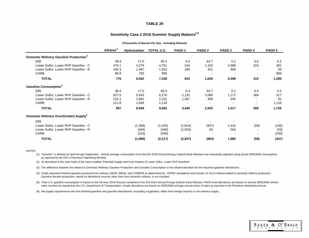
Ethanol 3Hydrocarbon TOTAL U.S. PADD 1 PADD 2 PADD 3 PADD 4 PADD 5
Domestic Refinery Gasoline Production4
E85 48.4 17.0 65.4 0.4 64.7 0.1 0.0 0.2 Lower Sulfur, Lower RVP Gasoline - C 475.1 4,276 4,751 319 1,153 2,589 310 381 Lower Sulfur, Lower RVP Gasoline - R 165.3 1,487 1,653 284 421 909 - 39 CARB 86.9 782 869 - - - - 869
TOTAL 776 6,562 7,338 603 1,639 3,498 310 1,289
Gasoline Consumption5
E85 48.4 17.0 65.4 0.4 64.7 0.1 0.0 0.2 Lower Sulfur, Lower RVP Gasoline - C 627.0 5,643 6,270 2,132 2,080 1,172 369 517 Lower Sulfur, Lower RVP Gasoline - R 210.1 1,891 2,101 1,307 358 345 - 91 CARB 111.8 1,006 1,118 - - - - 1,118
TOTAL 997 8,558 9,555 3,440 2,503 1,517 369 1,726
E85 - - - - - - - Lower Sulfur, Lower RVP Gasoline - C (1,368) (1,520) (1,814) (927) 1,416 (59) (136) Lower Sulfur, Lower RVP Gasoline - R (404) (449) (1,024) 63 564 - (53) CARB (224) (249) - - - - (249)
TOTAL (1,996) (2,217) (2,837) (864) 1,980 (59) (437)
NOTES:(1)
(2)
(3)
(5) Total U.S. gasoline consumption is based on the full year 2016 forecast contained in the EIA 2010 Annual Energy Outlook Early Release. PADD level allocations are based on annual 2005/2006 vehicle miles traveled as reported by the U.S. Department of Transportation. Grade allocations are based on 2005/2006 average annual share of sales as reported in the Petroleum Marketing Annual.
(6) Net supply requirements are from finished gasoline and gasoline blendstocks, excluding oxygenates, either from foreign imports or non-refinery supply.
The difference between the ethanol in Domestic Refinery Gasoline Production and Gasoline Consumption is the ethanol blended into the imported gasoline blendstocks.
(4)
TABLE 20
Sensitivity Case 2 2016 Summer Supply Balance1,2
(Thousands of Barrels Per Day - Including Ethanol)
Domestic Refinery Over/(Under) Supply6
"Summer" is defined as April through September. Annual average consumption from the EIA 2010 Annual Energy Outlook Early Release was seasonally adjusted using actual 2005/2006 consumption as reported by the EIA in Petroleum Marketing Monthly.
Totals represent finished gasoline produced from refinery CBOB, RBOB, and CARBOB as determined by PRISM simulations and include 10 Vol.% ethanol added to domestic refinery production. Gasoline blender production, based on blendstock sources other than from domestic refiners, is not included.
As described in the main body of the report entitled "Potential Supply and Cost Impacts of Lower Sulfur, Lower RVP Gasoline"

TOTAL U.S. PADD 1 PADD 2 PADD 3 PADD 4 PADD 5
Domestic Production by Crude Oil Refiners3
Total PoolRVP, psi 6.0 5.9 6.0 6.0 6.4 5.9Olefins, Vol.% 8.9% 10.4% 10.0% 9.3% 10.5% 5.4%Aromatics, Vol.% 30.9% 30.6% 31.6% 31.9% 29.1% 27.9%Benzene, Vol.% 0.61% 0.71% 0.72% 0.55% 0.75% 0.57%Sulfur, wppm 10.9 12.0 12.1 12.4 12.6 4.5
Lower Sulfur, Lower RVP Gasoline - CRVP, psi 6.3 6.4 6.2 6.2 6.4 6.3Olefins, Vol.% 10.2% 10.1% 10.6% 10.2% 10.5% 8.5%Aromatics, Vol.% 33.2% 37.5% 32.5% 33.4% 29.1% 33.2%Benzene, Vol.% 0.67% 0.71% 0.83% 0.58% 0.75% 0.75%Sulfur, wppm 11.8 10.8 12.2 12.5 12.6 6.7
Lower Sulfur, Lower RVP Gasoline - RRVP, psi 5.4 5.4 5.4 5.4 - 5.4Olefins, Vol.% 7.9% 10.7% 8.3% 7.0% - 4.6%Aromatics, Vol.% 27.3% 22.8% 28.9% 27.8% - 30.2%Benzene, Vol.% 0.52% 0.70% 0.44% 0.48% - 0.70%Sulfur, wppm 12.2 13.4 12.0 12.3 - 7.6
CARBOBRVP, psi 5.8 - - - - 5.8Olefins, Vol.% 4.0% - - - - 4.0%Aromatics, Vol.% 25.5% - - - - 25.5%Benzene, Vol.% 0.49% - - - - 0.49%Sulfur, wppm 3.4 - - - - 3.4
NOTES:(1)
(2)
(3) PRISM simulation results.
"Summer" is defined as April through September.
TABLE 21A
Sensitivity Case 2 2016 Summer Regional Finished Gasoline Qualities1,2
At Refinery Gate (Before Ethanol is Added)
As described in the main body of the report entitled "Potential Supply and Cost Impacts of Lower Sulfur, Lower RVP Gasoline"

TOTAL U.S. PADD 1 PADD 2 PADD 3 PADD 4 PADD 5
Domestic Production by Crude Oil Refiners3
Total PoolRVP, psi 7.4 7.3 7.4 7.4 7.7 7.3Olefins, Vol.% 8.0% 9.3% 9.0% 8.4% 9.5% 4.8%Aromatics, Vol.% 27.8% 27.5% 28.4% 28.8% 26.2% 25.1%Benzene, Vol.% 0.56% 0.64% 0.66% 0.50% 0.68% 0.52%Sulfur, wppm 10.8 11.8 11.9 12.2 12.3 5.1
Lower Sulfur, Lower RVP Gasoline - CRVP, psi 7.6 7.7 7.6 7.6 7.7 7.7Olefins, Vol.% 9.1% 9.1% 9.5% 9.1% 9.5% 7.6%Aromatics, Vol.% 29.9% 33.7% 29.3% 30.1% 26.2% 29.9%Benzene, Vol.% 0.61% 0.65% 0.75% 0.52% 0.68% 0.68%Sulfur, wppm 11.7 10.8 11.9 12.2 12.3 7.0
Lower Sulfur, Lower RVP Gasoline - RRVP, psi 6.9 6.9 6.9 6.9 - 6.9Olefins, Vol.% 7.1% 9.6% 7.5% 6.3% - 4.1%Aromatics, Vol.% 24.5% 20.5% 26.0% 25.0% - 27.1%Benzene, Vol.% 0.47% 0.64% 0.41% 0.44% - 0.64%Sulfur, wppm 12.0 13.0 11.8 12.0 - 7.9
CARBOBRVP, psi 7.2 - - - - 7.2Olefins, Vol.% 3.6% - - - - 3.6%Aromatics, Vol.% 23.0% - - - - 23.0%Benzene, Vol.% 0.45% - - - - 0.45%Sulfur, wppm 4.1 - - - - 4.1
NOTES:(1)
(2)
(3) PRISM simulation results.
"Summer" is defined as April through September.
TABLE 21B
Sensitivity Case 2 2016 Summer Regional Finished Gasoline Qualities1,2
(includes Ethanol)
As described in the main body of the report entitled "Potential Supply and Cost Impacts of Lower Sulfur, Lower RVP Gasoline"

TOTAL U.S. PADD 1 PADD 2 PADD 3 PADD 4 PADD 5
Domestic Production by Crude Oil Refiners3
E85 Gasoline 65.4 0.4 64.7 0.1 0.0 0.2 Lower Sulfur, Lower RVP Gasoline - C 4,751 319 1,153 2,589 310 381 Lower Sulfur, Lower RVP Gasoline - R 1,653 284 421 909 - 39 CARB Gasoline 869 - - - - 869 Jet Fuel 1,666 109 273 796 41 447 Distillates 4,251 285 960 2,311 177 518 Pentanes 437 40 78 225 6 88
Other4 4,135 434 756 2,153 41 751
TOTAL 17,826 1,471 3,705 8,982 574 3,094
NOTES:(1)
(2)
(4) Includes LPG, residual fuel oil, aviation gasoline, petrochemical feedstocks, lubricants, waxes, asphalt, road oil, still gas, special naphthas, petroleum coke, and miscellaneous petroleum products.
(3)
TABLE 22
Sensitivity Case 2 2016 Summer Production1,2
(Thousands of Barrels Per Day - Including Ethanol)
Totals represent finished gasoline produced from refinery CBOB, RBOB, and CARBOB as determined by PRISM simulations and include 10 Vol.% ethanol added to refinery production. Gasoline blender production, based on blendstock sources other than from domestic refiners, is not included.
"Summer" is defined as April through September. Annual average consumption from the EIA 2010 Annual Energy Outlook Early Release was seasonally adjusted using actual 2005/2006 consumption as reported by the EIA in Petroleum Marketing Monthly.
As described in the main body of the report entitled "Potential Supply and Cost Impacts of Lower Sulfur, Lower RVP Gasoline"

Ethanol 3Hydrocarbon TOTAL U.S. PADD 1 PADD 2 PADD 3 PADD 4 PADD 5
Domestic Refinery Gasoline Production4
E85 48.4 17.0 65.4 0.4 64.7 0.1 0.0 0.2 Lower Sulfur, Lower RVP Gasoline - C 501.2 4,510 5,012 331 1,232 2,730 324 394 Lower Sulfur, Lower RVP Gasoline - R 166.3 1,496 1,663 284 409 931 - 39 CARB 87.7 790 877 - - - - 877
TOTAL 804 6,813 7,617 615 1,706 3,662 324 1,311
Gasoline Consumption5
E85 48.4 17.0 65.4 0.4 64.7 0.1 0.0 0.2 Lower Sulfur, Lower RVP Gasoline - C 627.0 5,643 6,270 2,132 2,080 1,172 369 517 Lower Sulfur, Lower RVP Gasoline - R 210.1 1,891 2,101 1,307 358 345 - 91 CARB 111.8 1,006 1,118 - - - - 1,118
TOTAL 997 8,558 9,555 3,440 2,503 1,517 369 1,726
E85 - - - - - - - Lower Sulfur, Lower RVP Gasoline - C (1,133) (1,259) (1,801) (848) 1,558 (45) (122) Lower Sulfur, Lower RVP Gasoline - R (395) (439) (1,024) 51 586 - (53) CARB (216) (241) - - - - (241)
TOTAL (1,744) (1,938) (2,825) (797) 2,144 (45) (415)
NOTES:(1)
(3)
(5) Total U.S. gasoline consumption is based on the full year 2016 forecast contained in the EIA 2010 Annual Energy Outlook Early Release. PADD level allocations are based on annual 2005/2006 vehicle miles traveled as reported by the U.S. Department of Transportation. Grade allocations are based on 2005/2006 average annual share of sales as reported in the Petroleum Marketing Annual.
(6) Net supply requirements are from finished gasoline and gasoline blendstocks, excluding oxygenates, either from foreign imports or non-refinery supply.
The difference between the ethanol in Domestic Refinery Gasoline Production and Gasoline Consumption is the ethanol blended into the imported gasoline blendstocks.
(4)
TABLE 23
Sensitivity Case 3 2016 Summer Supply Balance1,2
(Thousands of Barrels Per Day - Including Ethanol)
Domestic Refinery Over/(Under) Supply6
"Summer" is defined as April through September. Annual average consumption from the EIA 2010 Annual Energy Outlook Early Release was seasonally adjusted using actual 2005/2006 consumption as reported by the EIA in Petroleum Marketing Monthly.
Totals represent finished gasoline produced from refinery CBOB, RBOB, and CARBOB as determined by PRISM simulations and include 10 Vol.% ethanol added to domestic refinery production. Gasoline blender production, based on blendstock sources other than from domestic refiners, is not included.
(2) As described in the main body of the report entitled "Potential Supply and Cost Impacts of Lower Sulfur, Lower RVP Gasoline"

TOTAL U.S. PADD 1 PADD 2 PADD 3 PADD 4 PADD 5
Domestic Production by Crude Oil Refiners3
Total PoolRVP, psi 6.6 6.3 6.7 6.7 7.5 6.2Olefins, Vol.% 9.6% 11.2% 9.8% 10.5% 10.1% 5.7%Aromatics, Vol.% 29.7% 29.6% 30.1% 30.5% 27.9% 27.5%Benzene, Vol.% 0.59% 0.69% 0.70% 0.53% 0.73% 0.56%Sulfur, wppm 10.8 11.8 12.0 12.2 12.1 4.5
Lower Sulfur, Lower RVP Gasoline - CRVP, psi 7.1 7.1 7.1 7.1 7.5 7.4Olefins, Vol.% 11.2% 11.5% 10.5% 11.8% 10.1% 10.1%Aromatics, Vol.% 32.2% 36.9% 30.8% 33.1% 27.9% 30.2%Benzene, Vol.% 0.63% 0.63% 0.80% 0.54% 0.73% 0.66%Sulfur, wppm 11.8 10.2 12.5 12.4 12.1 6.8
Lower Sulfur, Lower RVP Gasoline - RRVP, psi 5.4 5.4 5.4 5.4 - 5.4Olefins, Vol.% 7.6% 10.8% 7.8% 6.7% - 4.6%Aromatics, Vol.% 24.0% 21.1% 28.0% 22.9% - 30.2%Benzene, Vol.% 0.51% 0.77% 0.39% 0.48% - 0.70%Sulfur, wppm 11.6 13.8 10.4 11.7 - 7.6
CARBOBRVP, psi 5.8 - - - - 5.8Olefins, Vol.% 3.8% - - - - 3.8%Aromatics, Vol.% 26.1% - - - - 26.1%Benzene, Vol.% 0.51% - - - - 0.51%Sulfur, wppm 3.4 - - - - 3.4
NOTES:(1)
(3) PRISM simulation results.
"Summer" is defined as April through September.
TABLE 24A
Sensitivity Case 3 2016 Summer Regional Finished Gasoline Qualities1,2
At Refinery Gate (Before Ethanol is Added)
(2) As described in the main body of the report entitled "Potential Supply and Cost Impacts of Lower Sulfur, Lower RVP Gasoline"

TOTAL U.S. PADD 1 PADD 2 PADD 3 PADD 4 PADD 5
Domestic Production by Crude Oil Refiners3
Total PoolRVP, psi 7.9 7.7 8.0 7.9 8.7 7.6Olefins, Vol.% 8.6% 10.1% 8.8% 9.5% 9.1% 5.1%Aromatics, Vol.% 26.7% 26.6% 27.1% 27.4% 25.1% 24.7%Benzene, Vol.% 0.54% 0.63% 0.63% 0.48% 0.66% 0.51%Sulfur, wppm 10.7 11.6 11.8 12.0 11.9 5.1
Lower Sulfur, Lower RVP Gasoline - CRVP, psi 8.3 8.3 8.3 8.3 8.7 8.5Olefins, Vol.% 10.1% 10.4% 9.4% 10.6% 9.1% 9.1%Aromatics, Vol.% 29.0% 33.2% 27.7% 29.8% 25.1% 27.2%Benzene, Vol.% 0.57% 0.57% 0.72% 0.49% 0.66% 0.60%Sulfur, wppm 11.6 10.2 12.3 12.1 11.9 7.1
Lower Sulfur, Lower RVP Gasoline - RRVP, psi 6.9 6.9 6.9 6.9 - 6.9Olefins, Vol.% 6.8% 9.7% 7.0% 6.0% - 4.1%Aromatics, Vol.% 21.6% 19.0% 25.2% 20.6% - 27.1%Benzene, Vol.% 0.47% 0.70% 0.36% 0.44% - 0.64%Sulfur, wppm 11.5 13.4 10.4 11.5 - 7.9
CARBOBRVP, psi 7.2 - - - - 7.2Olefins, Vol.% 3.4% - - - - 3.4%Aromatics, Vol.% 23.5% - - - - 23.5%Benzene, Vol.% 0.46% - - - - 0.46%Sulfur, wppm 4.1 - - - - 4.1
NOTES:(1)
(3) PRISM simulation results.
"Summer" is defined as April through September.
TABLE 24B
Sensitivity Case 3 2016 Summer Regional Finished Gasoline Qualities1,2
(includes Ethanol)
(2) As described in the main body of the report entitled "Potential Supply and Cost Impacts of Lower Sulfur, Lower RVP Gasoline"

TOTAL U.S. PADD 1 PADD 2 PADD 3 PADD 4 PADD 5
Domestic Production by Crude Oil Refiners3
E85 Gasoline 65.4 0.4 64.7 0.1 0.0 0.2 Lower Sulfur, Lower RVP Gasoline - C 5,012 331 1,232 2,730 324 394 Lower Sulfur, Lower RVP Gasoline - R 1,663 284 409 931 - 39 CARB Gasoline 877 - - - - 877 Jet Fuel 1,667 109 273 796 41 448 Distillates 4,250 285 960 2,310 177 518 Pentanes 269 28 41 130 0 70
Other4 4,323 432 750 2,240 134 766
TOTAL 18,125 1,469 3,729 9,138 676 3,114
NOTES:(1)
(4) Includes LPG, residual fuel oil, aviation gasoline, petrochemical feedstocks, lubricants, waxes, asphalt, road oil, still gas, special naphthas, petroleum coke, and miscellaneous petroleum products.
(3)
TABLE 25
Sensitivity Case 3 2016 Summer Production1,2
(Thousands of Barrels Per Day - Including Ethanol)
Totals represent finished gasoline produced from refinery CBOB, RBOB, and CARBOB as determined by PRISM simulations and include 10 Vol.% ethanol added to refinery production. Gasoline blender production, based on blendstock sources other than from domestic refiners, is not included.
"Summer" is defined as April through September. Annual average consumption from the EIA 2010 Annual Energy Outlook Early Release was seasonally adjusted using actual 2005/2006 consumption as reported by the EIA in Petroleum Marketing Monthly.
(2) As described in the main body of the report entitled "Potential Supply and Cost Impacts of Lower Sulfur, Lower RVP Gasoline"

TOTAL U.S. PADD 1 PADD 2 PADD 3 PADD 4 PADD 5
Crude InputsBase Case 14,941 1,118 3,256 7,400 596 2,571 Study Case 14,511 1,118 3,111 7,293 596 2,393
Delta (430) - (145) (107) - (178) Delta, % -3% 0% -4% -1% 0% -7%
Total Refinery InputsBase Case 16,402 1,261 3,434 8,250 623 2,835 Study Case 15,864 1,262 3,257 8,077 610 2,657
Delta (538) 1 (177) (172) (13) (177) Delta, % -3% 0% -5% -2% -2% -6%
LSRBOB (excl. EtOH)3
Base Case 6,567 609 1,741 3,519 310 389 Study Case 5,501 523 1,346 3,015 258 359
Delta (1,066) (86) (395) (504) (51) (29) Delta, % -16% -14% -23% -14% -17% -8%
CARBOB (excl. EtOH)Base Case 868 - - - - 868 Study Case 776 - - - - 776
Delta (91) - - - - (91) Delta, % -11% -11%
DistillatesBase Case 5,733 410 1,156 3,012 211 944 Study Case 5,911 432 1,231 3,106 220 922
Delta 178 22 75 95 9 (22) Delta, % 3% 5% 6% 3% 4% -2%
Base Case (MMSCFD) 1,629.7 20.1 36.5 1,326.7 0.8 245.5 Study Case (MMSCFD) 1,793.6 28.4 64.8 1,424.5 1.5 274.5
Delta (MMSCFD)5 163.9 8.2 28.3 97.7 0.6 29.0 Delta, % 10% 41% 77% 7% 72% 12%
NOTES:(1) "Summer" is defined as April through September.
(2)
(3)
(4)
(5)
SOURCE: Baker & O'Brien PRISM simulations
Difference in reported delta values are due to rounding.
LSRBOB is Lower Sulfur, Lower RVP Gasoline Blend for Oxygenate Blending. Base Case includes E85 hydrocarbon, CBOB and RBOB and the Study Case includes E85 hydrocarbon and LSRBOB.
Refinery Hydrogen Purchases is the total hydrogen purchased by domestic refineries to produce fuels.
TABLE 26
Study Case vs. Base Case Summer 20161,2
(Thousands of Barrels Per Day Unless Otherwise Stated)
As described in the main body of the report entitled "Potential Supply and Cost Impacts of Lower Sulfur, Lower RVP Gasoline"
Refinery Hydrogen Purchases4

TOTAL U.S. PADD 1 PADD 2 PADD 3 PADD 4 PADD 5
Crude InputsBase Case 14,941 1,118 3,256 7,400 596 2,571 Sensitivity Case 1 14,328 1,118 3,046 7,140 596 2,428
Delta (613) - (210) (260) - (143) Delta, % -4% 0% -6% -4% 0% -6%
Total Refinery InputsBase Case 16,402 1,261 3,434 8,250 623 2,835 Sensitivity Case 1 15,679 1,266 3,191 7,918 612 2,693
Delta (723) 5 (243) (332) (11) (142) Delta, % -4% 0% -7% -4% -2% -5%
LSRBOB (excl. EtOH)3
Base Case 6,567 609 1,741 3,519 310 389 Sensitivity Case 1 5,293 511 1,308 2,865 255 355
Delta (1,274) (98) (433) (654) (54) (34) Delta, % -19% -16% -25% -19% -18% -9%
CARBOB (excl. EtOH)Base Case 868 - - - - 868 Sensitivity Case 1 765 - - - - 765
Delta (103) - - - - (103) Delta, % -12% -12%
DistillatesBase Case 5,733 410 1,156 3,012 211 944 Sensitivity Case 1 5,844 434 1,222 3,063 225 900
Delta 111 23 66 51 14 (43) Delta, % 2% 6% 6% 2% 7% -5%
Base Case (MMSCFD) 1,618.4 20.1 36.5 1,315.4 0.8 245.5 Sensitivity Case 1 (MMSCFD) 1,911.2 46.3 93.5 1,469.3 1.5 300.5
Delta (MMSCFD)5 292.8 26.2 57.0 153.9 0.6 55.0 Delta, % 18% 130% 156% 12% 74% 22%
NOTES:(1) "Summer" is defined as April through September.
(2)
(3)
(4)
(5)
SOURCE: Baker & O'Brien PRISM simulations
Difference in reported delta values are due to rounding.
LSRBOB is Lower Sulfur, Lower RVP Gasoline Blend for Oxygenate Blending. Base Case includes E85 hydrocarbon, CBOB and RBOB and the Sensitivity Case 1 includes E85 hydrocarbon and LSRBOB.
Refinery Hydrogen Purchases is the total hydrogen purchased by domestic refineries to produce fuels.
TABLE 27
Sensitivity Case 1 vs. Base Case Summer 20161,2
(Thousands of Barrels Per Day Unless Otherwise Stated)
As described in the main body of the report entitled "Potential Supply and Cost Impacts of Lower Sulfur, Lower RVP Gasoline"
Refinery Hydrogen Purchases4

TOTAL U.S. PADD 1 PADD 2 PADD 3 PADD 4 PADD 5
Crude InputsBase Case 14,941 1,118 3,256 7,400 596 2,571 Sensitivity Case 2 14,511 1,118 3,111 7,293 596 2,393
Delta (430) - (145) (107) - (178) Delta, % -3% 0% -4% -1% 0% -7%
Total Refinery InputsBase Case 16,402 1,261 3,434 8,250 623 2,835 Sensitivity Case 2 15,860 1,260 3,255 8,075 612 2,658
Delta (543) (1) (178) (175) (11) (177) Delta, % -3% 0% -5% -2% -2% -6%
LSRBOB - C (excl. EtOH)3
Base Case 4,941 286 1,430 2,558 310 357 Sensitivity Case 2 4,293 287 1,054 2,330 279 343
Delta (649) 1 (375) (229) (31) (14) Delta, % -13% 0% -26% -9% -10% -4%
LSRBOB - R (excl. EtOH)4
Base Case 1,626 322 311 961 32 Sensitivity Case 2 1,487 255 379 818 - 35
Delta (138) (67) 68 (143) - 3 Delta, % -9% -21% 22% -15% - 11%
CARBOB (excl. EtOH)Base Case 868 - - - - 868 Sensitivity Case 2 782 - - - - 782
Delta (86) - - - - (86) Delta, % -10% -10%
DistillatesBase Case 5,733 410 1,156 3,012 211 944 Sensitivity Case 2 5,917 394 1,233 3,107 218 966
Delta 184 (17) 77 95 7 22 Delta, % 3% -4% 7% 3% 3% 2%
Base Case (MMSCFD) 1,629.7 20.1 36.5 1,326.7 0.8 245.5 Sensitivity Case 2 (MMSCFD) 1,814.4 28.3 64.5 1,416.6 0.8 304.1
Delta (MMSCFD)6 184.7 8.2 28.0 89.9 - 58.6 Delta, % 11% 41% 77% 7% 0% 24%
NOTES:(1) "Summer" is defined as April through September.
(2)
(3)
(4)
(5)
(6)
SOURCE: Baker & O'Brien PRISM simulations
Difference in reported delta values are due to rounding.
LSRBOB - C is Lower Sulfur, Lower RVP Gasoline Blend for Oxygenate Blending. Base Case includes E85 hydrocarbon, CBOB and the Sensitivity Case 2 includes E85 hydrocarbon and LSRBOB - C.
Refinery Hydrogen Purchases is the total hydrogen purchased by domestic refineries to produce fuels.
TABLE 28
Sensitivity Case 2 vs. Base Case Summer 20161,2
(Thousands of Barrels Per Day Unless Otherwise Stated)
As described in the main body of the report entitled "Potential Supply and Cost Impacts of Lower Sulfur, Lower RVP Gasoline"
Refinery Hydrogen Purchases5
LSRBOB - R is Lower Sulfur, Lower RVP Gasoline Blend for Oxygenate Blending. Base Case includes RBOB and the Sensitivity Case 2 includes

TOTAL U.S. PADD 1 PADD 2 PADD 3 PADD 4 PADD 5
Crude InputsBase Case 14,941 1,118 3,256 7,400 596 2,571 Sensitivity Case 3 14,511 1,118 3,111 7,293 596 2,393
Delta (430) - (145) (107) - (178) Delta, % -3% 0% -4% -1% 0% -7%
Total Refinery InputsBase Case 16,402 1,261 3,434 8,250 623 2,835 Sensitivity Case 3 15,923 1,258 3,271 8,119 617 2,658
Delta (479) (3) (163) (131) (5) (177) Delta, % -3% 0% -5% -2% -1% -6%
LSRBOB - C (excl. EtOH)3
Base Case 4,941 286 1,430 2,558 310 357 Sensitivity Case 3 4,527 298 1,126 2,457 291 355
Delta (414) 12 (304) (101) (18) (2) Delta, % -8% 4% -21% -4% -6% -1%
LSRBOB - R (excl. EtOH)4
Base Case 1,626 322 311 961 32 Sensitivity Case 3 1,496 255 368 838 35
Delta (129) (67) 57 (123) - 3 Delta, % -8% -21% 18% -13% - 11%
CARBOB (excl. EtOH)Base Case 868 - - - - 868 Sensitivity Case 3 790 - - - - 790
Delta (78) - - - - (78) Delta, % -9% -9%
DistillatesBase Case 5,733 410 1,156 3,012 211 944 Sensitivity Case 3 5,916 394 1,233 3,106 218 966
Delta 183 (17) 77 95 7 23 Delta, % 3% -4% 7% 3% 3% 2%
Base Case (MMSCFD) 1,629.7 20.1 36.5 1,326.7 0.8 245.5 Sensitivity Case 3 (MMSCFD) 1,814.6 28.3 64.5 1,416.5 0.8 304.4
Delta (MMSCFD)6 184.9 8.2 28.0 89.8 - 58.9 Delta, % 11% 41% 77% 7% 0% 24%
NOTES:(1) "Summer" is defined as April through September.
(2)
(3)
(4)
(5)
(6)
SOURCE: Baker & O'Brien PRISM simulations
Difference in reported delta values are due to rounding.
LSRBOB - C is Lower Sulfur, Lower RVP Gasoline Blend for Oxygenate Blending. Base Case includes E85 hydrocarbon, CBOB and the Sensitivity Case 3 includes E85 hydrocarbon and LSRBOB - C.
Refinery Hydrogen Purchases is the total hydrogen purchased by domestic refineries to produce fuels.
TABLE 29
Sensitivity Case 3 vs. Base Case Summer 20161,2
(Thousands of Barrels Per Day Unless Otherwise Stated)
As described in the main body of the report entitled "Potential Supply and Cost Impacts of Lower Sulfur, Lower RVP Gasoline"
Refinery Hydrogen Purchases5
LSRBOB - R is Lower Sulfur, Lower RVP Gasoline Blend for Oxygenate Blending. Base Case includes RBOB and the Sensitivity Case 3 includes