Pouring Liquids: A Study in Commonsense Physical Reasoning · PDF filefrom one container to another, ... and demonstrates that this inference and other similar inferences can be

Pouring Liquids:

A Study in Commonsense Physical Reasoning

Ernest Davis∗

Dept. of Computer Science

New York University

[email protected]

June 23, 2010

Abstract

This paper presents a theory that supports commonsense, qualitative reasoning about the

flow of liquid around slowly moving solid objects; specifically, inferring that liquid can be poured

from one container to another, given only qualitative information about the shapes and motions

of the containers. It shows how the theory and the problem specification can be expressed in

a first-order language; and demonstrates that this inference and other similar inferences can be

justified as deductive conclusions from theory and the problem specification.

Keywords: Liquids, qualitative physical reasoning, naive physics, qualitative spatial reasoning.

1 Introduction

Carrying liquids in containers and pouring or ladling liquids from one container to another areamong the most common ways in which people interact with liquids in daily life. People are veryfamiliar with these phenomena and can reason about them easily. In particular, people understandhow the physical behavior of the liquids is largely determined by the geometrical characteristics ofthe liquid, the containers, and the motions involved; they can reason about physical behavior usingonly partial knowledge of the geometry, without full geometric specifications; and they can use thesame knowledge in multiple inferential directions.

For instance, people know that, if a cup has a small hole through the bottom, then liquid inthe cup will leak out through the hole, but that a dent in the bottom will not cause the liquid toleak. They can use this knowledge in many ways: prediction — given that there is a hole, predictthat the liquid will leak; explanation — given that the liquid is leaking from the bottom, deducethat there is a hole; design — if you want the liquid to drain (e.g. you are designing a colander),put a hole in the bottom; and so on. These various forms of reasoning can be carried out withoutknowing or positing a precise shape description for the cup or the hole.

It is very desirable that an automated reasoner likewise be able to deal with partial geometricinformation. Precise geometric information may be unavailable for a number of different reasons.

∗I am grateful to the reviewers for many helpful suggestions. This research was supported in part by NSF grantIIS-0534809.

1

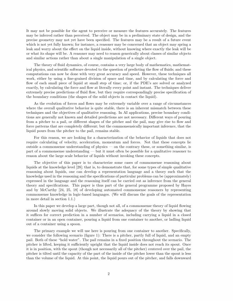
It may not be possible for the agent to perceive or measure the features accurately. The featuresmay be inferred rather than perceived. The object may be in a preliminary state of design, and theprecise geometry may not yet have been specified. The features may be a result of a future eventwhich is not yet fully known; for instance, a reasoner may be concerned that an object may spring aleak and worry about the effect on the liquid inside, without knowing where exactly the leak will beor what its shape will be. A reasoner may need to reason generically about classes of similar objectsand similar actions rather than about a single manipulation of a single object.

The theory of fluid dynamics, of course, contains a very large body of mathematics, mathemat-ical physics, and scientific software devoted to the question of predicting the flow of fluids; and thesecomputations can now be done with very great accuracy and speed. However, these techniques allwork, either by using a fine-grained division of space and time, and by calculating the force andflow of each small piece of liquid at small step of time; or, if the PDE’s are solved or analyzedexactly, by calculating the force and flow at literally every point and instant. The techniques deliverextremely precise predictions of fluid flow, but they require correspondingly precise specification ofthe boundary conditions (the shapes of the solid objects in contact the liquid).

As the evolution of forces and flows may be extremely variable over a range of circumstanceswhere the overall qualitative behavior is quite stable, there is an inherent mismatch between thesetechniques and the objectives of qualitative reasoning. In AI applications, precise boundary condi-tions are generally not known and detailed predictions are not necessary. Different ways of pouringfrom a pitcher to a pail, or different shapes of the pitcher and the pail, may give rise to flow andforce patterns that are completely different; but the commonsensically important inference, that theliquid pours from the pitcher to the pail, remains stable.

For this reason, we are looking for a characterization of the behavior of liquids that does notrequire calculating of velocity, acceleration, momentum and forces. Not that these concepts lieoutside a commonsense understanding of physics — on the contrary these, or something similar, ispart of a commonsense understanding — but it must often be possible for a qualitative reasoner toreason about the large scale behavior of liquids without invoking these concepts.

The objective of this paper is to characterize some cases of commonsense reasoning aboutliquids at the knowledge level [28]; that is, to demonstrate that, for some types of simple qualitativereasoning about liquids, one can develop a representation language and a theory such that theknowledge used in the reasoning and the specifications of particular problems can be (approximately)expressed in the language and the reasoning itself can be carried out as inference from the generaltheory and specifications. This paper is thus part of the general programme proposed by Hayesand by McCarthy [24, 25, 18] of developing automated commonsense reasoners by representingcommonsense knowledge in logic-based languages. (We will discuss the goals of the representationin more detail in section 1.1.)

In this paper we develop a large part, though not all, of a commonsense theory of liquid flowingaround slowly moving solid objects. We illustrate the adequacy of the theory by showing thatit suffices for correct prediction in a number of scenarios, including carrying a liquid in a closedcontainer or in an open container, pouring a liquid from one container to another, or ladling liquidout of a container using a spoon.

The primary example we will use here is pouring from one container to another. Specifically,we consider the following scenario (figure 1): There is a pitcher, partly full of liquid, and an emptypail. Both of these “hold water”. The pail remains in a fixed position throughout the scenario. Thepitcher is lifted, keeping it sufficiently upright that the liquid inside does not reach its spout. Onceit is in position, with the spout (though not necessarily all of the pitcher) centered over the pail, thepitcher is tilted until the capacity of the part of the inside of the pitcher lower than the spout is lessthan the volume of the liquid. At this point, the liquid pours out of the pitcher, and falls downward

2

��

��

��

��

��

��

��

��

��

��

��

��

��

��

��

��

��

��

��

��

Pail Pitcher

Figure 1: Pouring from pitcher to pail

into the pail, where it remains. At the end of the scenario, the liquid is divided into a section thatremains in the pitcher and a section that is in the pail. We demonstrate that, given qualitativecharacterizations of the shapes of the pitcher and the pail and of the motion of the pitcher, ourtheory allows us to infer the behavior of the liquid.

(Note: all of the figures in this paper are cross-sections in the x-z plane. Throughout thispaper, solid objects are indicated with diagonal lines, and liquid is indicated in grey. The fact thatthe pictures show liquid flowing in polygonal patterns reflects my personal limitations in using thedrawing software; it is not at all a requirement of the theory.)

Many aspects of the commonsense understanding of liquids are omitted from our analysis here.Some of the most important of these are:

• Liquids in modes that are not “bulk”, in Hayes’ [19] terminology, such as mists, wettings ofsurfaces, liquids absorbed in sponges, and so on.

• Liquids in energetic modes, again in Hayes’ terminology, such as fountains or even splashes.

• Mixtures or solutions of any kind.

• Interactions of liquids with the atmosphere or other gasses.

• The effect of liquids on the solids with which they are in contact. We assume that the motionof the solids is given by external constraints. Thus, our theory does not include waterwheelsor other mechanisms controlled by hydraulics, solid objects floating on liquids, swimming, andso on. (The theory may be capable in such cases of predicting the liquid flow given the motionof the solid objects, but it certainly cannot predict the motion of the solid objects.)

• Pressure and any consequences of pressure differences. In particular, we assume that all partsof the top surface of a liquid meet the open atmosphere and are therefore at equal height.

• Viscosity, surface tension, cohesion, adhesion, absorption, and so on. We deal only with “drywater”, in von Neumann’s sardonic phrase.

• Any consideration of heat, temperature, and phase transitions, such as evaporation and freez-ing.

• The feasibility of actions by an agent. The theory developed for physical feasibility of actionson solid objects in [11] can be extended to this domain, but we will not discuss this in thispaper.

3

• The theory yields incorrect predictions for liquids flowing down a channel (section 6). This isprobably the most important gap in the theory.

The paper is organized as follows. Section 1.1 discusses the various goals of this representa-tional work in more detail. Section 2 reviews previous relevant work. Section 3 gives a pre-formalaccount of the physical theory that we develop here. Section 4 shows how the theory can be formal-ized; it presents the ontology, the formal language, and the axioms. Section 5 describes a problemspecification for a scenario of carrying a liquid in a pitcher and pouring it into a pail; sketches thestructure of the formal inference; and demonstrates that the axioms and specifications are consistentby exhibiting a specific model satisfying them. (A complete formal proof of the inference is givenin the online appendix http://www.cs.nyu.edu/faculty/davise/papers/liqAppa.pdf.) Section 6 dis-cusses the problem of flow in a channel, which is a major gap in this theory. Section 7 presents theconclusion and discusses possible next steps for research.

1.1 Objectives

This paper undertakes a representational project with the following parts:

• We define a microworld of solid objects and liquids, which includes many of the basic large-scale behaviors of liquids carried in solid containers, poured out of and into solid containers,and flowing over solids. We state a number of physical laws that govern the behavior of liquidin the microworld.

• We develop a formal ontology and a first-order representation language in which we can for-mally state these laws.

• Extending this representation language with some additional geometric predicates, we con-struct a specification of a scenario of a pitcher pouring liquid into a pail with incompletegeometric specifications of the shapes and motions of the pitcher and the pail. We demon-strate that, from the rules and the specifications, we can infer that some of the liquid poursfrom the pitcher.

Of course, the physical theory is not intended to apply only to this particular specification; it shouldapply to many different specifications and different directions of inference within this microworld,and we are quite confident that it does (section 5.3).

There are many ways in which such a representational project could be carried out, and numer-ous different desiderata for the theory and for the problem specification:

1. The theory and specifications should be logically sufficient. The conclusion must beprovable from the specifications and the physical theory.

2. The specifications should be qualitative. It would be (comparatively) easy to give geo-metrically precise descriptions of shape and motion that would suffice to justify the conclusion.But that kind of inference can be done much better — more precisely, robustly, and generally— by conventional simulation methods. The whole point of the theory we have developed isthat it supports reasoning from incomplete specifications. Other things being equal, the moregeneral the specifications the better.

3. The theory should be general. The theory should not apply only to the problem inquestion but to a wide range of problems in the microworld. It should be usable not only forprediction but also for other directions of inference (postdiction, planning, design, etc.)

4

4. The specifications for a prediction problem should be geometric. A well-formedprediction problem should consist of specifications of the shape of the objects; the initial stateof the liquid; constraints on the motion of the objects; and isolation conditions excludingoutside interference (no other object or liquid comes close to the scene of the action). This isessentially the “No function in structure” rule of [15].

5. Specifications should be logically simple and use fixed geometric vocabulary. Ina knowledge base that uses this representation, the general theory corresponds to the fixedknowledge base whereas the specification corresponds to the run-time query. Therefore, com-plex logical form or specialized predicates may be tolerable in the theory, since these can beincorporated off-line into workable algorithms, but it is important that queries in the spec-ification language be logically simple combinations of known predicates (e.g. conjunction ofground formulas) if there is to be any hope of achieving run-time efficiency.

6. The specifications should be ecologically valid. The constraints should correspond tothe kinds of partial information that are available in actual applications, or should be easilyderivable from that information.

7. The theory and specifications should be computationally tractable. It should bepossible for a program to draw the desired inferences from the specifications in reasonable time.Until there is a corpus of examples and a proposal on the table for an inference algorithm,there is no way to evaluate this. The theoretical worst-case results are all discouraging; spatiallanguages much more restricted than this one are intractable or undecidable [2].

8. The theory should bear some relation to physical reality. The theory should beapproximately correct, or correct in the limit in some sense, or correct as an average in somesense, or in one way or another correspond to the physical reality. A theory with physicallyvery unrealistic assumptions is likely to go very badly wrong sooner or later.

9. The theory should be plausible as a cognitive model. To the extent that this can bejudged reliably, it should be plausible that the predicates correspond to concepts available tonaive human reasoners. It should be noted that almost nothing is known about what conceptsare used for qualitative physical reasoning by human reasoners, so it would be a mistake to letone’s own guesses on the subject dictate the form of one’s theory.

10. It is desirable that the predicates should be standard in computational geometry. .It would be helpful, though it is not critical, if the geometric predicates used were well-knownand well-understood in the literatures of computational geometry, graphics, CAD, physics,scientific computing etc. so that we could draw on methods from those disciplines and interfaceeasily with them.

The theory and problem specifications developed in this paper presented below certainly satisfycondition 1-4 and, in their current form, certainly do not satisfy condition 7. On the whole we havevery much favored achieving the generality advocated in condition 3 over conditions 6-10. In mostrespects, the theory is approximately physically correct (condition 8); in some aspects, which we willpoint out, the approximation is quite crude. Condition 5 is hard to evaluate until many differenttypes of problems have been formalized, which we have not yet done. Some of the predicates in ourrepresentation are standard (condition 10); many as far as I know as new here and of very limitedapplicability.

As regards cognitive plausibility (condition 9): At first blush it would seem absurd to claim anydegree of cognitive plausibility for a theory with concepts like “continuity relative to the Hausdorffdistance” (section 3.7) or “bubble-free attachment” (section 5). But the truth is that the common-sensical human reasoner has some conceptualization of the fact that liquids move continuously and of

5

the geometric relation between a container and an opening. The formal definitions here are intendedas mathematical definitions that idealize or approximate the intuitive conception, and though theformal definition is not very readable, I would argue that the actual concept is reasonably close.That is, this jargon is just a translation of the intuitive conceptualization of “continuous liquid mo-tion” into “math-talk”, and, it seems to me, a reasonably close translation. The major physical rulesthat are developed in this paper. (section 3.1) are, I would argue, quite reasonable candidates for acognitive model, though the details are designed in part to avoid the need for plausible reasoning,which a true cognitive model would, of course, deal with. At minimum, it seems to me that theconcepts and rules here constitute a worthwhile first stab at a cognitive theory of the domain. I donot claim that the cognitive processes involved at all resemble the formal proofs in the appendix.

The important sticking point here is condition 6. As argued at length in [8], though it is clearthat many AI applications require reasoning from partial information, it is not at all easy to know,for a given application, exactly what kinds of partial information are involved; and it is often veryhard, for a given domain of interest, to find an application that naturally generates a collection ofinferences from partial information to satisfy the requirements of condition 4. It is obvious thatpeople can reason about pouring liquid from a pitcher without knowing the precise shape of thepitcher; it is much harder to say what it is they do know about the pitcher. Moreover, in realisticapplications, some of the information that is available may not satisfy either condition 1 or condition3 above. For instance, one may know “I have often poured liquid from this pitcher without trouble”or “The text refers to this object as a ‘pitcher’; hence, it is presumably possible to pour from it.”But clearly neither of these facts support very strong deductive conclusions, nor are they geometric.

2 Related Work

It is unusual, particularly in a fast-moving field like AI, for a survey of previous related work tobe dominated by a single paper — Pat Hayes’ “Ontology for Liquids” [19], a companion paper toHayes’ “Naive Physics Manifesto” [18] – which was written almost thirty years ago,1 immediatelybecame very famous, and has barely been touched from then to now.

Besides proposing liquids as a challenging and fruitful domain for research in automated com-monsense physical reasoning, and proposing as an initial step the axiomatization of the domain ina first-order language, “Ontology for Liquids” made a number of critical contributions. The mostimportant of these (certainly in terms of its influence on this paper) was to show that a criticalcategory in reasoning about liquids is that of a region of space that evolves over time, and that suchan evolving region should be considered as an entity in the domain of discourse. (Hayes calls this a“history”, whereas in this paper it is called a “region-valued fluent”.) Other important contributionsof Hayes’ paper include:

• The categorization of different modes of liquids, in a commonsense understanding, along four,largely independent, dimensions: bulk vs. divided, still vs. moving and lazy vs. energetic,unsupported vs. supported, in an extended space vs. close to a surface. (Of the 24 logicalcombinations, Hayes claims that 15 are physically possible.)

• The development of a qualitative language of geometry guided by the demands of a physicaltheory. This is one of the earliest works in AI on qualitative geometry, and, despite all thesubsequent work in this area [2], still one of comparatively few that is designed to fit witha physical theory. (DeKleer’s NEWTON [14] predates it in both respects, but is much morelimited in both the geometry and the physics.)

1“Ontology for Liquids” was written as a working paper in 1979 and circulated in photocopies for six years beforeit was published in 1985.

6

Moreover, the discussion in “Ontology for Liquids” is in many respects broader than this paper.Hayes touches on such subjects as the fifteen modes of liquids mentioned above, liquids adhering tosurfaces, solid objects floating on liquids, and others, which we do not consider here.

However, the logic presented in “Ontology for Liquids” has substantial gaps and flaws. Themost serious of these is that, in developing his representation, Hayes assumes that “Almost all thehistories we consider in this paper . . . consist[] of a certain piece of space in which something happensfor a certain length of time; they are rectangular” ([19], p. 90). Both the representation and theaxiomatization depend strongly on this assumption. But the two examples he considers (a bathtuboverflowing, a liquid flowing from a tilted container onto a surface) do not at all correspond to thisassumption; almost none of the significant histories involved are rectangular. For that reason, it isactually impossible to fill in the details of the logical analysis of these examples given in section 9of “Ontology for Liquids”. This gap is very much obscured for the reader (and, probably, for Hayeshimself) by the fact that Hayes does not give a logical statement of the specification of the problemsbeing addressed in section 9.2

Rectangular histories are the norm only when the system is in the steady-state, and over theclass of steady-state histories, Hayes’ theory is indeed often adequate. But pouring is not a steady-state system, and rectangular histories do not come close to dealing adequately with it.

Another problem, which as we shall see arises also with theories of very different kinds, hasto do with the physics of overflowing. As we shall discuss in more detail in section 3, when anopen container overflows at the top, the liquid necessarily rises somewhat above the top of thecontainer and spills out some horizontal distance beyond the edge of the container. Neither of theseis consistent with Hayes’ theory. In particular, as soon as a liquid goes beyond the edge of thecontainer, then it must fall straight down; therefore, it cannot travel outward any finite distance.

2.1 Other AI theories of liquids

A number of other AI theories have dealt with geometrically and physically rich models of liquids.Gardin and Meltzer [17] simulate liquids in terms of particles interacting in a two-dimensionalspace (one vertical and one horizontal). They also simulate rigid objects, flexible objects, andstrings in the same way. Obviously, no such representation can deal adequately with qualitativespatial reasoning. Less obviously, the rules of physical interaction they propose lead to a systemwhose behavior is determined by the grain-size of the discretization of time and space. (In standardscientific computation, as the grain-size becomes increasingly fine, the predictions hopefully convergeon the actual behavior.) Specifically, in the “pouring” scenario, once a particle of water has gonepast the lip of the pitcher, it is unsupported, and therefore must fall straight down. The resultis that the liquid pours out of the pitcher in a column one molecule thick. (This is quite clearlyillustrated in [17] p. 679, figure 19.10.)

DeCuyper et al. [13] point out, correctly, some of the limitations of Hayes’ analysis, particularlyin terms of the spatial language, and propose a hybrid architecture for reasoning about liquidscombining three representations: a particle-based representation which tracks the movement ofparticles of liquid; a fixed grid partition of space which tracks the occupancy of each voxel of space,and a qualitative representation similar to Hayes’. They do not give the details, and, frankly, itseems unlikely that this was ever worked out in detail. It is not difficult to imagine a system thatcan compute a simulation and abstract a qualitative representation, though this is certainly a non-

2This gap was also critical to the debate over Hayes’ argument between McDermott in his “Critique of Pure Reason”[26] and Hayes in his response [20]. McDermott claimed that Hayes’ bathtub examples required non-monotonicreasoning; Hayes claimed that they required only modus tollens. The truth is that, in the absence of a specificproblem specification, there is no way to know which closed world assumptions are to be considered part of theproblem specification, and which are to be considered as deduced using non-monotonic principles.

7

trivial challenge; but it is very difficult to devise a system in which there is significant informationflow in the opposite direction, from the qualitative analysis to the simulation.

Kim [21] developed a system that carried out qualitative predictions of the motions of liquidsin response to the motions of pistons. She also included in her model a special case of solids beingacted on by liquids, namely the opening and closing of one-way valves. Both the geometric andphysical language of this system were quite limited.

Many AI physical reasoning systems have used a geometry-free model of liquids, characterizingthe state of liquid purely in terms of the quantity of liquid contained in specified containers, andcharacterizing flow just as a process that decreases the quantity in the source and increases thequantity in the destination. For instance Forbus [16] uses this as an example for qualitative predic-tion; Shin and Davis [34] use it as an example for planning with quantities that are linear functionsof time (the system assume that all flows are constant-rate). Collins and Forbus [3] combine thiswith a model of liquids in terms of collections of molecules, which supports some more sophisticatedinferences.

2.2 Logical theories of commonsense physical domains

The work described in this paper is part of an ongoing project to develop formal theories of com-monsense physical domains. This work is mostly presented in three previous papers.

In [4] I presented a formal theory of a very small part of solid object dynamics, capable ofsupporting the inference that a marble dropped inside a funnel would come out the bottom. Themost significant technical innovation here is the concept of a “pseudo-object”, a geometric entitythat “moves around” with a rigid object, such as the hole of a doughnut or the center of mass of anobject (section 4.5). This theory has been very much extended in [11], which supports the conclusionthat a collection of objects can be loaded into a box and then carried in the box. That paper, unlikethis one, includes an explicit theory of manipulation by an agent.

An axiomatization of a kinematic model of one solid object cutting another is given in [7]. Twotheories are presented. The “object” theory views the process of a blade cutting a target object asinvolving a continuous change in the shape of the target until it splits, when it becomes two objects.The “chunk” theory views the same process in terms of the chunks of solid material contained inthe target. (Every separate region defines a separate chunk.) A chunk persists until it is penetratedby the blade, at which point it ceases to exist. These chunks are closely analogous to the “liquidchunks” studied in this paper.

All of these theories are mutually compatible, and I hope to present them in an integrated formin a monograph currently under preparation [12].

I have also done other, more minor and less well integrated, work on the formalization of physicalreasoning.

Chapter 7 of [5] gives preliminary axiomatizations for a number of physical domains, includingliquids. An axiomatization of qualitative process theory is given in [6]. The main issue here is toformulate the closed world assumptions correctly.

The methodological paper [8] advocates structuring domain theories around microworlds ratherthan clusters, as proposed in Hayes’ “Naive Physics Manifesto” [18].

Other than the above, there has been little work on logical formalizations of physical domainssince Hayes’ original papers, despite their fame and popularity. Schmolze [32] presents an axioma-tization for a domain that includes actions, events, processes, liquids, solid containers, and faucets.A liquid is modelled as a collection of “granules”.

8

Sandewall [31] developed a logical description of a microworld of points objects moving alongsurfaces. The chief focus of this work was integrating non-monotonic logic with a continuous modelof time. Fluents were assumed non-monotonically to be continuous at each point in time; thus amodel with a minimal class of discontinuities was preferred.

Three parallel papers by Lifschitz, Morgenstern, and Shanahan [23, 27, 33] axiomatize variousaspects of the process of cracking an egg into a bowl.

Bennett et al. [1] present an axiomatization of solid object kinematics built up from geometricalprimitives.

2.3 Fluid dynamics

The elephant in the room here, which I can neither ignore nor adequately deal with, is the immense,deep, and sophisticated mathematical and computational theory of fluid dynamics. It would requireyears of study to gain a sufficient mastery of this field to be confident that the problems I am studyingcannot be solved by existing techniques; or that an expert in the field could not develop a theory ofpower comparable to the one here, but grounded in standard fluid dynamics. Such a theory wouldby definition be more physically correct than the one here; it would almost certainly be easier tointegrate with standard methods of physical calculation; it might well be more extensible, easily tovalidate for consistency, perhaps even a more plausible cognitive model. All I can say is that I havenot found any evidence that the kind of reasoning studied in this paper has been addressed in theexisting theory of fluid dynamics, or indeed is of any interest to researchers in fluid dynamics. As faras I have been able to determine, none of the techniques that have been developed in fluid dynamicscan be applied at all directly to the kinds of qualitative information that we are considering here.

3 The Physical Theory

The physical theory developed in this paper deals with the motion of liquid around slowly movingsolid objects. We begin with a high-level sketch of the theory (section 3.1); we then work througha detailed formulation of our proposed physical rules. (section 3.2–3.5). Section 3.6 discusses theontology of liquids. Section 3.7 discusses the constraint that liquids move continuously.

3.1 The Physical Theory: High-level view

Our ontology, like Hayes’, has two dual categories that we use to characterize the motion of liquids.The first category is region-valued fluents (Hayes calls these “histories”): fluents whose value at eachtime is a region, such as “the region contained inside pitcher P1”. Many aspects of liquid motioncan be characterized in terms of the quantity of liquid contained in significant region-valued fluents,but some aspects, such as steady-state flow or cyclic flow, cannot. The second category is bodies orpieces or chunks of liquid (we will use these terms interchangeably). A piece of liquid is a particularcollection of matter; a set of molecules, if you like, though our theory is not based on molecules.Thus we can say, “Some of the piece of liquid that was in the pitcher at the start of the scenario isin the pail at the end of the scenario.” By contrast, in the language of region-based fluents all thatwe can say is that at the end of the scenario there is less liquid in the pitcher and more liquid inthe pail than at the beginning. To say that that the liquid that is in the pail at the end is the sameas the liquid that was in the pitcher at the start and is no longer in the pitcher requires an identitycriterion on liquid over time, and thus requires the category of pieces of liquid. Hayes prefers usinghistories to using pieces of liquids; we use the two concepts about equally.

9

��

��

��

��

��

��

R

Figure 2: Region R is cupped

Essentially, our theory of liquids consists of the following rules:

Rule 1. Liquids cannot interpenetrate solid objects.

Rule 2. The volume of a particular body of liquid is constant (incompressibility).

Rule 3. The motion of liquid through space is continuous over time (we will define the sense of “con-tinuity” required here in section 3.7).

Rule 4. A connected region R is said to be “cupped” at a given time if the outside of the boundary ofR consists of solid objects everywhere except at a top, horizontal surface (figure 2). If a region(more precisely, a region-valued fluent) R is cupped over a period of time and is never full ofliquid, then no liquid flows out of R.

Rule 5. If a body of liquid can flow straight down without encountering a solid object or a cuppedliquid, then it does flow straight down.

Rule 6. If a body of liquid is in contact with a solid or cupped liquid but can flow downward aroundit, then it does flow downward around it.

Given these rules, one can (informally) justify the analysis of the pouring scenario as follows:By rule 4, the liquid remains in the pitcher as the pitcher is lifted into position. By rule 2, oncethe volume inside the pitcher below the spout falls below the volume of the liquid, the liquid can nolonger be held in the pitcher; since the pitcher prevents it from flowing out the bottom or out thesides (rule 1), it flows out the top. At this point, the part of the liquid above the top of the spoutcannot flow straight downward because of the cupped liquid underneath it, but it can flow at anangle downward over the spout following rule 6. Once it has cleared the spout, it can flow straightdownward, so it does so by rule 5. This brings it inside the pail. Once it is inside the pail, it cannotescape by rule 4.

The objective here is to formulate these rules in a way that they are mutually consistent, strongenough to predict the result of the pouring scenario, and flexible enough to be usable with qualitativespatial information.

The first problem is that the overflow of the pitcher in the pouring scenario necessarily con-tradicts rules 5 and 6. If liquid pours out of a spout, then it must necessarily flow up somewhathigher than the level of the spout and flow out horizontally somewhat beyond the spout (figure 3).Suppose that the liquid rises to height DH over the top of the spout and flows out to a distanceDW beyond the spout. Then at the earlier time when it had only flowed out to distance DW/2beyond the spout it could have flowed straight down, and should have, if rule 5 applied. Likewise,at the time when the liquid had risen to height DH/2 above the spout, it should have started toflow downward over the spout if rule 6 applied, and not have continued to flow upward.

In a continuous model, such as we will use here, this leads to a Zeno-like paradox. In a moleculartheory, it leads to the conclusion that the liquid rises one molecule about the level of the spout and

10

��

��

DH

DW

Figure 3: Flowing over and past of the spout

��

��

Figure 4: Overflow past a precipice

then pours out in a column one molecule thick. As mentioned above, this is exactly the conclusionthat Gardin and Meltzer’s program does come to [17].

The same problem can arise in any situation where a flow over an object turns into free flow.If a liquid has been flowing down a slanted surface, and then comes to a precipice (figure 4) thenit must flow some distance beyond the edge before falling straight down, but, again, if it does flowa finite distance beyond the edge, then it is violating rule 5 by not starting to flow straight downsooner.

Finally, the problem arises, though in a less clear-cut form, when a downward flow terminatesin an object. If a vertical column of liquid is flowing downward and hits a surface, then any part ofthe liquid above the object can flow downward and by rule 5 must do so; but it is not possible thatthe horizontal flow of the liquid begins exactly at the surface.

The true explanation here, of course, involves the momentum of the liquid; but as we havediscussed, we wish if possible to avoid reasoning paths that require reasoning about momentum.Instead, what we will do here is to posit that these kinds of scenarios generate exceptions to rules 5and 6.

This solution in turn raises two further difficulties. The first is that, in a monotonic logic suchas we use here, if one has stated that a rule has exceptions, then ever after, in order to apply the

11

rule, one must ascertain that the exception does not hold. As we shall see, this places demands bothon the domain axiomatization and on the problem specification.

The second, more important, problem is that some limits must be given on how far, spatially,these exceptions extend: How far can liquid rise above the wall of a cup before it is required to flowdown, and how far horizontally can it flow out beyond the rim of a cup before it is required to flowstraight down? These are necessary, first because it is obviously the case that liquid in this scenariocannot flow indefinitely far up or out, and more specifically because this conclusion is necessary tocarry out the desired inference. If we cannot bound how far the liquid flows beyond the spout of thepitcher, then we cannot predict that it will flow into the pail; it may overshoot the pail.

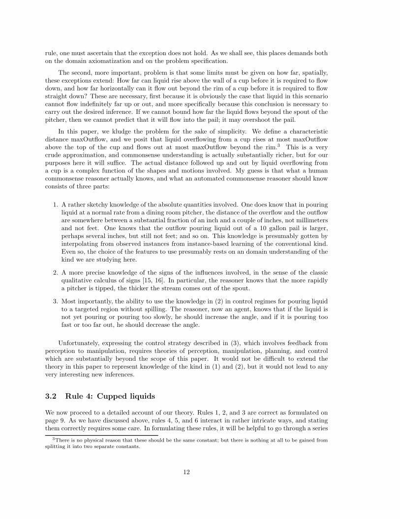
In this paper, we kludge the problem for the sake of simplicity. We define a characteristicdistance maxOutflow, and we posit that liquid overflowing from a cup rises at most maxOutflowabove the top of the cup and flows out at most maxOutflow beyond the rim.3 This is a verycrude approximation, and commonsense understanding is actually substantially richer, but for ourpurposes here it will suffice. The actual distance followed up and out by liquid overflowing froma cup is a complex function of the shapes and motions involved. My guess is that what a humancommonsense reasoner actually knows, and what an automated commonsense reasoner should knowconsists of three parts:

1. A rather sketchy knowledge of the absolute quantities involved. One does know that in pouringliquid at a normal rate from a dining room pitcher, the distance of the overflow and the outfloware somewhere between a substantial fraction of an inch and a couple of inches, not millimetersand not feet. One knows that the outflow pouring liquid out of a 10 gallon pail is larger,perhaps several inches, but still not feet; and so on. This knowledge is presumably gotten byinterpolating from observed instances from instance-based learning of the conventional kind.Even so, the choice of the features to use presumably rests on an domain understanding of thekind we are studying here.

2. A more precise knowledge of the signs of the influences involved, in the sense of the classicqualitative calculus of signs [15, 16]. In particular, the reasoner knows that the more rapidlya pitcher is tipped, the thicker the stream comes out of the spout.

3. Most importantly, the ability to use the knowledge in (2) in control regimes for pouring liquidto a targeted region without spilling. The reasoner, now an agent, knows that if the liquid isnot yet pouring or pouring too slowly, he should increase the angle, and if it is pouring toofast or too far out, he should decrease the angle.

Unfortunately, expressing the control strategy described in (3), which involves feedback fromperception to manipulation, requires theories of perception, manipulation, planning, and controlwhich are substantially beyond the scope of this paper. It would not be difficult to extend thetheory in this paper to represent knowledge of the kind in (1) and (2), but it would not lead to anyvery interesting new inferences.

3.2 Rule 4: Cupped liquids

We now proceed to a detailed account of our theory. Rules 1, 2, and 3 are correct as formulated onpage 9. As we have discussed above, rules 4, 5, and 6 interact in rather intricate ways, and statingthem correctly requires some care. In formulating these rules, it will be helpful to go through a series

3There is no physical reason that these should be the same constant; but there is nothing at all to be gained fromsplitting it into two separate constants.

12

R2 R3 R3R1

R1 and R2 are thickly connected. R3 (the union of the two outer brackets) is not.

Figure 5: Thickly connected regions

of approximations; that is, we will first state the rule in a form that is nearly correct, explain thecases in which it works, explain the cases it doesn’t work, revise the rule, and if necessary iterate.

We begin our formulation of rule 4 with a few basic definitions,

Definition 3.2.1: A region is a topologically regular4 set of points in ℜ3, not necessarilyeither connected or bounded. A region-valued fluent is a function from time to regions.

Definition 3.2.2: A region R is thickly connected if the interior of R is connected(figure 5).

Definition 3.2.3: A region R is cupped at time T if:

1. R is thickly connected;

2. No solid object overlaps R;

3. Any boundary point of R that is lower than the highest point in R is a boundary pointof some solid object.

Thus the boundary of a cupped region R consists of (a) a horizontal top surface (possiblydisconnected, but of constant height) where R meets the open air; and (b) the rest of the boundary,where R is bounded by solid objects. Note that the cupped region may be formed by a single solidobject or by many.

We can now formulate a first approximation to rule 4:

Rule 4.A: Let Q be a region-valued fluent. Suppose that over time interval I, Q isalways cupped and is a continuous function of time. (Again, we defer to section 3.7 thequestion of what it means to say that a function of time to regions is “continuous”.) IfQ is never full of liquid in I, then there is no outflow from Q during I.

Before explaining the problem with this formulation and correcting it, let me first discuss acouple of critical aspects of the proposed rule, and then show that this rule works correctly in somecases where one might suppose there was a problem.

First, when we say that liquid L “flows out of” fluent Q during time interval I, what that meansis at some time in I, L is inside Q, and at some later time in I, L is outside Q. This can happen,either because the liquid L moves, or because Q moves, or both.

Second, the chief feature of rule 4.A is that it applies to all region-valued fluents that arecontinuous and always cupped, not just the largest-possible cup in each state. For instance, infigure 6, one might define the following fluents:

4A set of points is regular if it is equal to the closure of its interior. The regularization of set S is the closure ofthe interior of S.

13

��

��

��

��

��

��

��

��

Q1

Q2Q2

Q3

Q1Q1

Q1,Q3

Q2Q2Q3

S1 S2

S3 S4

Q3

Figure 6: Fluents onto cupped regions for Rule 4

• Q1 is the largest cupped region formed by the cup.

• Q2 is the cupped region whose top is always 8 inches below the top of Q1.

• Q3 is the cupped region whose top is always 8 inches above the bottom of the cup

All of these satisfy the conditions of continuity and of always being cupped. There are infinitelymany such fluents. The condition that Q is not full of liquid is met by Q1 throughout the scenario;it is met by Q2 from states S1 to S2, and ends sometime between S2 and S3; it is met by Q3 fromS1 to S2, becomes false in S2, and becomes true again some time between S3 and S4. During thetime that it is met, for a given fluent, the rule states that no liquid flows out of the fluent, which isclearly the case. The point is that, since the fluent Q is always cupped, any flow out of Q can onlycome out of the top of Q; and the liquid inside Q only reaches the top of Q if its volume becomesequal to the volume of Q.

Third, the boundaries of the cup can be formed either by a single object, as in the pitcherexample, or by several objects; in fact, the collection of objects that form the cup can vary overtime, as long as the interior of the cup is a continuous function of time. For example, if you droppebbles into a vase, then the “cupped region” is the interior of the vase minus the pebbles; the rulethen states that as long as the volume of the liquid is less than the volume of the vase minus thevolume of the pebbles, the vase will not overflow. Or one might have a cup formed by a cylinder

14

��

��

��

��

��

��

��

��

��

��

��

��

��

��

��

��

��

��

Figure 7: Cylinder with piston

��

��

��

��

��

��

��

��

��

��

��

��

S1 S2 S3

Figure 8: Ladling from a pail

and a piston that can move the bottom of the cupped region up and down (figure 7); this will be auseful example for us in our discussion, since it is easier to see what happens to the volume of thecup in this case than in the case of a tilting pitcher. In all these cases, we assume that the liquidinside the cup can always reshape itself to the interior of the cup as fast as the objects move around;this is part of the assumption that objects move slowly.

One might suppose that a scenario like figure 8, in which liquid is lifted out of a pail in a ladle,would contradict rule 4.A. After all, the interior of the pail is a cupped region and the liquid inthe ladle comes out of the pail even though the interior of the pail is not full of liquid. But in factthere is no problem here. The interior of the pail, minus the solid material of the ladle, does indeedconstitute a cupped region in state S1, and continues to do so right until state S2, when the rim ofthe ladle reaches the top of the pail. At that moment, however, the interior of the pail as a wholeceases to be a cupped region, because it ceases to be thickly connected. In S2 there are two separatecupped region: One region that is inside the pail and outside the ladle and one region that is insidethe ladle, and there is no cupped region that includes them both. Therefore, the fluent “inside ofthe pail minus the material of the ladle” does not satisfy the conditions of the lemma, since it is notcupped in S2 and after.

One might also suppose that inflow into a cupped region could cause trouble for the rule; surelyif there is liquid flowing into a region there can be liquid flowing out of it? The answer is no; therecan be outflow only if the region is full of liquid, in which case the condition of the rule is notsatisfied.

15

��

��

��

��

��

��

��

��

��

��

��

��

��

��

��

��

Figure 9: Exception to rule 4.A

The cases where the rule does fail are more recondite. Consider the case shown in figure 9: thepiston cup, full of liquid, is inside an empty pail and the piston is pushed upward. Suppose thatthe motion of the piston causes the liquid to rise a distance DH over the top of the cylinder. Nowconsider the region bounded by the pail whose top is DH/2 above the top of the cylinder. Thisfluent does violate rule 4.A; it is always cupped, it is a continuous function of time, it is not full ofliquid, and yet liquid flows out.

We therefore have to make an exception to rule 4.A in the case of a cupped region that containsanother cupped region that is overflowing. Specifically, we say that a piece of liquid is “driven” ifit is overflowing from a cup (the precise definition is given in the next sentence). Driven liquids areexceptions to rules 4, 5, and 6.

We now can formulate rule 4 correctly:

Rule 4. Let Q be a region-valued fluent. Suppose that over time interval I, Q is alwayscupped, is a continuous function of time, and does not contain any driven liquids. If Qis never full of liquid in I, then there is no outflow from Q during I.

3.3 Driven Liquids

To complete the formulation of rule 4, we need next to define precisely what is meant by a “driven”liquid. This definition, as we will see, constitutes our theory of overflowing; overflow occurs in theregion above the top of a cup where a driven liquid is allowed to violate rules 4, 5, and 6.

The definition that we will present is obviously rather arbitrary and does not correspond closelyto any physical reality. Given the nature of the theory here, this arbitrariness is, I think, bothinevitable and unimportant. It is inevitable, because we are trying to characterize what is a verycomplex, dynamic process in terms of a few simple geometric constraints; necessarily, the fit will notbe very good. And it is unimportant because the question of exactly what is happening at the layerwhere liquid is overflowing is probably not very well understood by human commonsense reasoner,and does not much affect the large-scale inference that the liquid pours from the pitcher into thepot. What is important is that the rule should be stated in a way that (a) successfully resolves thecontradiction between the unqualified version of rules 4, 5, and 6 and the scenario of an overflowingcup; and (b) justifies the inference that overflow liquid pouring from a spout can only go a fairlysmall distance before rule 5 starts to apply and the liquid pours straight downward.

Since driven liquid is caused by an overflowing cupped region, we must first characterize the

16

��

��

��

��

��

��

��

��

��

��

��

��

��RA

Figure 10: Not a case of overflow

circumstance of overflowing. Unlike rule 4, which applies to all cupped regions, it is not the case thatoverflowing occurs whenever any cupped region becomes too small for the liquid it contains. Forinstance, in figure 10, the liquid reaches the top of RA and rises above it, but there is no overflow,in the sense of an exception to rules 4, 5, and 6; the liquid just continues to occupy the cuppedregion of the correct volume at the current bottom of the cylinder. True overflow and driven liquidoccurs when it is not possible for the liquid to adjust instantaneously to a new bottom of a cup,either because it is not inside any cupped region at all any more, or because the nearest containingcupped region is some finite distance beyond the overflowing cup, and the liquid requires some finitetime to flow out to it.

We are thus led to the definition of a locally maximal cup:

Definition 3.3.1: Region R is a locally maximal cup at time T if:

1. R is a cupped region at T .

2. There exists a distance D > 0 such that, if R1 is a cupped region in S and R1 properly containsR, then some point in R1 is at least distance D from R.

Thus, RA in figure 10 is not a locally maximal cup, since there are cupped regions that aresupersets of RA and arbitrarily close to RA. By contrast, the inside of the ladle in figure 8 and theinside of the cylinder in figure 9 are locally maximal cups, because the cupped regions that properlycontain them all involve the inside of the pail and thus contain points that are far from the insideof the ladle/cylinder.

Definition 3.3.2: Let Q be a region-valued fluent that, throughout time interval [TS, TE], iscontinuous and is always a locally-maximal cup. If Q is full at TS, and the volume of Q strictlymonotonically decreases throughout [TS, TE], then Q overflows throughout I.

Definition 3.3.3: Let Q be a region-valued fluent that overflows throughout time interval [TS, TE].Let T be a time between TS and TE, and let Q(T ) be the value of Q at T . Suppose that a pieceof liquid L fills region R at T . L is driven by the overflow from Q at T (figure 11) if:

1. R ∪ Q(T ) is thickly connected.

2. R is entirely within distance maxOutflow of Q(T ).

3. For every point P in R there is a point P ′ in Q(T ) such that the line from P to P ′ is entirelyin R and the height of P ′ is less than or equal to the height of P .

Note that in these definitions, the liquid overflowing from Q is driven only as long as the volume

17

��

��

��

��

��

��

��

��

RBRAmaxOutflow

Regions RA and RB are driven regions

Figure 11: Driven regions

of Q is monotonically decreasing; as soon as Q stops decreasing in volume, the overflow ceases to bedriven and starts being governed by rules 4 and 5.

3.4 Rule 6: Flowing down

Definition 3.4.1: A liquid L flows down during a time interval if the heights of the top and of thebottom of L are monotonically strictly decreasing functions of time.

Rule 6: If a piece of liquid L can flow down at time T , then it does flow down.

The question is, what do we mean by saying that a liquid “can flow down”? Rather thananalyze this in terms of a general theory of possible behaviors of liquids, which raises rather difficulttechnical issues, we will give an an explicit geometric characterization.

Definition 3.4.2: At any time T , nonFlowingSpace is the union of all regions of space occupied bysolid objects, cupped liquids, driven liquids, and “weakly cupped” liquids.

A liquid is weakly cupped if it is cupped by some combination of solid objects and driven liquid.Since driven liquid is, to a degree, resistant to being pushed out of the way, weakly cupped liquidmust likewise be, since there is nowhere it can flow to except into the driven liquid.

Definition 3.4.3 Point P is a flow stopping point associated with region R if P is a local minimumof the top surface of R. (R is the region occupied by an obstacle. A liquid incident on P cannotflow downward at P .)

Definition 3.4.4: A piece of liquid L cannot flow down if either L overlaps nonFlowingSpace or ifa bottom point of L is incident on a flow stopping point of nonFlowingSpace. If it is not the casethat L cannot flow down, then L can flow down.

If a piece of liquid L can flow down, in the sense of definition 3.4.3 then either there is nothingbelow it, or it can flow around whatever is below it, or whatever is below it is itself flowing downand thus making room for L.

Suppose, for instance, that in a given coordinate system there is a fixed solid table with a roundhorizontal top of radius 2 lying in the x-y plane at z=0, and suppose that there is a cylinder of water

18

��

��

Figure 12: Column of liquid flowing down

of radius 1 and height 1 sitting above the center of the table at time t=0. By our definition anypiece of this cylinder that is incident on the table cannot flow down; any piece that is not incidenton the table can flow down. And indeed, assuming that the cylinder flows outward and downward,every piece not incident on the table will flow down (figure 12). Consider, for example, the followingflow pattern: a point of liquid whose position at t = 0 is 〈r0, θ0, z0〉 in cylindrical coordinates att = 0 flows to position 〈r0/

√1 − t, θ0, z0(1 − t)〉 for t between 0 and 3/4 (at t = 3/4 the liquid

reaches the edge of the table). It is easily verified that in this flow pattern every piece of liquid hasa constant volume, and move continuously, and that every piece of liquid not incident on the tableflows downward.

3.5 Rule 5: Flowing straight downward

There are two main questions about rule 5. First, what is the dividing line between regions whererule 5 applies and regions where only rule 6 applies? Second, what is meant by the statement thata liquid “flows straight down”?

As regards the first question: As with our definition of “driven liquid” in section 3.3, ourdefinition here is rather arbitrary, justified on the grounds that in this kind of theory precision isneither possible nor necessary.

Definition 3.5.1: At time T , R is a flow disruption region if the following hold:

1. R is thickly connected.

2. R is filled with liquid.

3. For every point P in R, there is a point P ′ at the top of nonFlowingSpace such thatheight(P ) ≥ height(P ′); P is within maxOutflow of P ′; and the line from P to P ′ does not gothrough any solid objects.

Definition 3.5.2: The region flowDisruptedSpace is the union of all flow disruption regions. Theregion flowUndisruptedSpace is the complement of flowDisruptedSpace ∪ nonFlowingSpace.

As regards “flowing straight down”: The obvious interpretation of “flows straight down” wouldbe a simple vertical translation downward. However, it is obviously impossible to have a steadyflow of liquid in a column that (a) translates straight downward; (b) preserves volume; (c) does notbreak into droplets; and (d) accelerates under gravity. Rather, if (b), (c), and (d) hold, then the

19

stream of flowing liquid must get narrower, and indeed this is what happens. But if the stream isgrowing narrower, then the parts of the liquid at the periphery are not translating straight down,they are moving toward the center. It is not necessary, at our level of precision, to have a theorythat mandates that falling liquid accelerates, but it seems overly restrictive to have a theory thatprohibits it. Therefore we define “falling straight down” as a characteristic, not of all pieces ofliquids, but of a stream as a whole (or, more precisely, of a horizontal slice of a stream.)

Definition 3.5.3: A piece of liquid L falls straight down if it falls downward and the horizontalprojection of L is a monotonically non-increasing function of time. (The complete statement of thisdefinition requires an additional condition to ensure continuity. See section 4.9.)

Rule 5: At time T , let L be any piece of liquid in flowUndisruptedSpace. Then Lis contained in a piece of liquid LX with the same vertical span that flows straightdownward for some time interval starting in T .

3.6 The Ontology of Liquids

There are a number of different ontologies that can be used for modelling the dynamics of liquidflow:

I. Discrete models

I.1 Molecular model. A quantity of liquid on the scale of easy manipulations (between about1 gram and 100 kilograms) consists of between about 1022 and 1027 molecules, interactingthrough van der Waals forces.

I.2 Small particle model. Liquid consists of a collection of particles that are very small on thehuman scale but very large as compared to a molecule. They are too small, and thereforetoo numerous, to allow reasoning that depends on enumerating them individually, butlarge enough that each one can be meaningfully assigned properties that are in factstatistics over large numbers of molecules, such as temperature [3].5

I.3 Large particle model. The behavior of liquid can be calculated by simulating the in-teractions of a fairly small number (dozens or at most hundreds) of large-scale particles[17].

I.4 Spatial cellular model. Space is divided into a grid of cells, and the state of the liquid ischaracterized in terms of the occupancy of the cells.

II. Continuous models

II.1 Fixed point model. The behavior of the liquid is characterized in terms of the evolvingstate of the liquid at fixed points in space. (This is the Eulerian model in fluid dynamics.)

II.2 Flowing point model. The behavior of the liquid is characterized by tracking “points” ofliquid as they move through space over time, and describing the position of each pointand the state of the liquid at the point. (This is the Lagrangian model in fluid dynamics.)For instance, the specification of fluid flow in section 3.4 is a simple instance of a flowingpoint model.

II.3 Fixed region models. The behavior of the liquid is characterized in terms of the occupancyof fixed regions.

5Gibbs used a somewhat similar model in order to apply statistical mechanic arguments to thermodynamics withoutneeding to resolve the ongoing controversy over the kinetic model of heat.

20

II.4 Pieces of liquid. The behavior of the liquid is characterized in terms of the motion ofpieces of liquid over time.

Hayes’ theory [19] uses primarily the fixed regions model and to a lesser extent the “pieces ofliquid” model. Kim’s program [21] likewise uses primarily the fixed regions model. DeCuyper et al.[13] propose a hybrid architecture combining a large particle model, a spatial cellular model, and afixed region model, but as mentioned it seems unlikely that the details of this were ever worked out.As our above discussion indicates, our theory here uses primarily the “pieces of liquids” model andto a lesser extent the fixed regions model.

Space here does not permit an extended comparison of these ontologies, but let me discussbriefly the difficulties that arise in using the other ontologies for the kinds of reasoning addressedhere.

The true molecular model I.1 is of course the most correct of these; but it is by far the mostdifficult to use. The relationship between the small scale interactions of the molecules and the largescale dynamics of liquid is mediated by statistical mechanics, and the reasoning needed to get fromone to the other is generally more complex than the kinds of reasoning used in this paper or incontinuous fluid dynamics.

The small particle discrete model of [3] was developed to enable rather specific lines of inference;for instance, to reason about liquid that heats up while flowing past a heat source. No generaldynamic theory has been developed using this ontology.

The large particle model and the cellular model are both inherently limited in their precisionby the grain-size of the discretization. Neither is applicable in any straightforward way to reasoningwith qualitative spatial information.

It should be noted that the large particle model is no less an abstraction of the true molecularmodel than any of the other models described here; and it is a mistake to suppose that the superficialresemblance between the large particle model and the molecular model implies that there is anyactual advantage to using the large particle model in reasoning. A collection of 1023 moleculesactually behaves in almost every respect more like the partial differential equations of fluid dynamicsthan like a collection of 100 particles.

The two point-based models II.1 and II.2 are the basis of fluid dynamics. They have the advan-tages, first, that an exact specification of flow and other dynamic change can easily be representedin terms of closed-form formulas, as we have done in above in section 3.4; and that a very precisedynamic theory can be stated in partial differential equations. However, neither of these is suitedto qualitative reasoning. The evolution of the flow field and the partial derivatives involved areunstable under the kind of qualitative variation we wish to consider, even in circumstances wherethe overall behavior is very stable.

Note, also, that even in stating the standard scientific theory, there are facts that are moreeasily stated in the region-based ontology than in point-based ontologies. In particular, the incom-pressibility of liquid is trivial to state in the region-based model. In the flowing point model, it issubstantially more complicated to state, and in the fixed point model, it can only be stated quiteindirectly, using the divergence theorem.

Ideally, one would think that there ought to be a language for describing large-scale physicalphenomena that is agnostic and indifferent to the small-scale structure. After all, the naive humanreasoner knows how liquids behave on the scales in which he can perceive and manipulate it and heneither knows nor cares what is going on at scales much smaller than he can perceive; a commonsensetheory should do likewise, certainly if it is making claims to cognitive validity. Unfortunately, despitemany attempts, no one has succeeded in formulating such a theory. Space here does not permit ananalysis of the difficulties involved; I hope to address this in [12].

21

a1

b1 a3

a2 b2

Figure 13: Measures of distance between regions

3.7 Continuous motion of liquids

An important constraint on liquids is that they move continuously in space. In a “piece of liquid”ontology, it is not obvious how this constraint should be expressed, since there are a number ofdifferent possible topologies over the space of regions, and hence a number of different notions ofcontinuity [9].

One condition that is indisputable is that the volume of liquid in any bounded region must be acontinuous function of time; e.g. the volume of liquid in a pail cannot instantaneously change from1 pint to 2 pints. This can be guaranteed as follows:

Definition 3.7.1: Let R1 and R2 be two bounded, topologically regular regions. The symmetricdifference of R1 and R2, denoted R1⊖R2 is defined as the regularization of (R1−R2)∪ (R2−R1).We define the function dV (R1, R2) =volume(R1 ⊖ R2).

For example, let A be the square with vertices 〈1, 1〉, 〈−1, 1〉〈−1,−1〉, 〈1,−1〉 and let B be thecircle centered at the origin of radius 1.2 (figure 13). The symmetric difference between A and B

consists of the four corners of the square that lie outside the circle together with the four “sides” ofthe circle that lie outside the square. The area of this region is 0.92.

It is easily shown that dV is a metric over the space of regular, bounded regions.

Definition 3.7.2: Let Q be a region-valued fluent and let I be a time interval. Q is volume-continuous during I if it is continuous with respect to the metric dV ; that is, for any ǫ > 0 thereexists δ > 0 such that, for all T 1, T 2 in I, if |T 1 − T 2| < δ then dV (Q(T 1), Q(T 2)) < ǫ.

It is certainly the case that the region occupied by any piece of liquid is volume-continuous overtime. However, this constraint is too weak; it would permit a liquid to gradually disappear from onecontainer and simultaneously reappear in a container some distance away. Such a behavior wouldbe volume-continuous but is clearly not what we mean by liquid moving continuously.

22

��

��

��

��

��

��

��

��

��

��

��

��

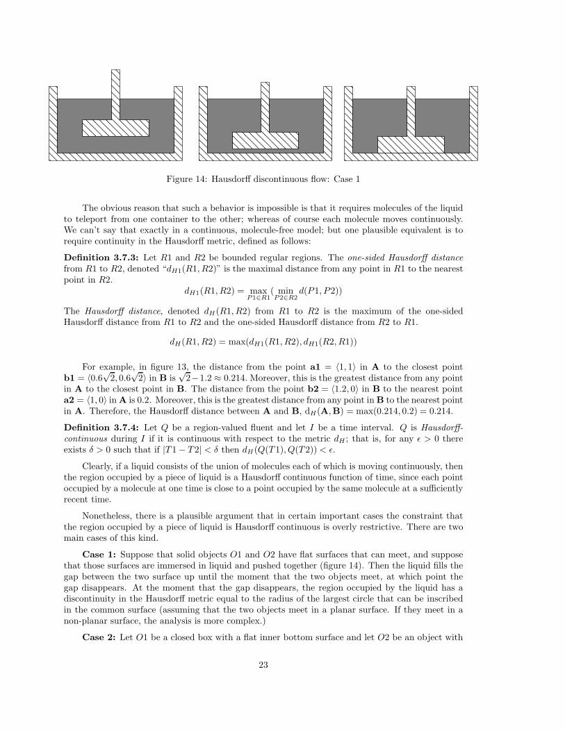
Figure 14: Hausdorff discontinuous flow: Case 1

The obvious reason that such a behavior is impossible is that it requires molecules of the liquidto teleport from one container to the other; whereas of course each molecule moves continuously.We can’t say that exactly in a continuous, molecule-free model; but one plausible equivalent is torequire continuity in the Hausdorff metric, defined as follows:

Definition 3.7.3: Let R1 and R2 be bounded regular regions. The one-sided Hausdorff distancefrom R1 to R2, denoted “dH1(R1, R2)” is the maximal distance from any point in R1 to the nearestpoint in R2.

dH1(R1, R2) = maxP1∈R1

( minP2∈R2

d(P1, P2))

The Hausdorff distance, denoted dH(R1, R2) from R1 to R2 is the maximum of the one-sidedHausdorff distance from R1 to R2 and the one-sided Hausdorff distance from R2 to R1.

dH(R1, R2) = max(dH1(R1, R2), dH1(R2, R1))

For example, in figure 13, the distance from the point a1 = 〈1, 1〉 in A to the closest pointb1 = 〈0.6

√2, 0.6

√2〉 in B is

√2−1.2 ≈ 0.214. Moreover, this is the greatest distance from any point

in A to the closest point in B. The distance from the point b2 = 〈1.2, 0〉 in B to the nearest pointa2 = 〈1, 0〉 in A is 0.2. Moreover, this is the greatest distance from any point in B to the nearest pointin A. Therefore, the Hausdorff distance between A and B, dH(A,B) = max(0.214, 0.2) = 0.214.

Definition 3.7.4: Let Q be a region-valued fluent and let I be a time interval. Q is Hausdorff-continuous during I if it is continuous with respect to the metric dH ; that is, for any ǫ > 0 thereexists δ > 0 such that if |T 1 − T 2| < δ then dH(Q(T 1), Q(T 2)) < ǫ.

Clearly, if a liquid consists of the union of molecules each of which is moving continuously, thenthe region occupied by a piece of liquid is a Hausdorff continuous function of time, since each pointoccupied by a molecule at one time is close to a point occupied by the same molecule at a sufficientlyrecent time.

Nonetheless, there is a plausible argument that in certain important cases the constraint thatthe region occupied by a piece of liquid is Hausdorff continuous is overly restrictive. There are twomain cases of this kind.

Case 1: Suppose that solid objects O1 and O2 have flat surfaces that can meet, and supposethat those surfaces are immersed in liquid and pushed together (figure 14). Then the liquid fills thegap between the two surface up until the moment that the two objects meet, at which point thegap disappears. At the moment that the gap disappears, the region occupied by the liquid has adiscontinuity in the Hausdorff metric equal to the radius of the largest circle that can be inscribedin the common surface (assuming that the two objects meet in a planar surface. If they meet in anon-planar surface, the analysis is more complex.)

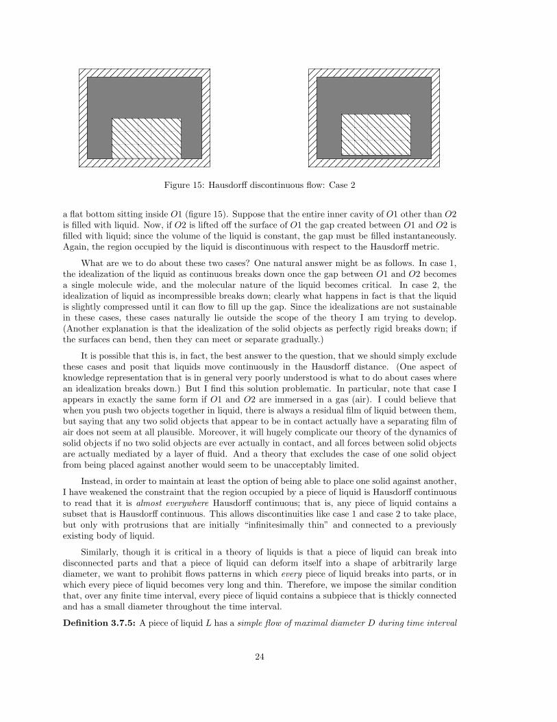
Case 2: Let O1 be a closed box with a flat inner bottom surface and let O2 be an object with

23

��

��

��

��

��

��

��

��

Figure 15: Hausdorff discontinuous flow: Case 2

a flat bottom sitting inside O1 (figure 15). Suppose that the entire inner cavity of O1 other than O2is filled with liquid. Now, if O2 is lifted off the surface of O1 the gap created between O1 and O2 isfilled with liquid; since the volume of the liquid is constant, the gap must be filled instantaneously.Again, the region occupied by the liquid is discontinuous with respect to the Hausdorff metric.

What are we to do about these two cases? One natural answer might be as follows. In case 1,the idealization of the liquid as continuous breaks down once the gap between O1 and O2 becomesa single molecule wide, and the molecular nature of the liquid becomes critical. In case 2, theidealization of liquid as incompressible breaks down; clearly what happens in fact is that the liquidis slightly compressed until it can flow to fill up the gap. Since the idealizations are not sustainablein these cases, these cases naturally lie outside the scope of the theory I am trying to develop.(Another explanation is that the idealization of the solid objects as perfectly rigid breaks down; ifthe surfaces can bend, then they can meet or separate gradually.)

It is possible that this is, in fact, the best answer to the question, that we should simply excludethese cases and posit that liquids move continuously in the Hausdorff distance. (One aspect ofknowledge representation that is in general very poorly understood is what to do about cases wherean idealization breaks down.) But I find this solution problematic. In particular, note that case Iappears in exactly the same form if O1 and O2 are immersed in a gas (air). I could believe thatwhen you push two objects together in liquid, there is always a residual film of liquid between them,but saying that any two solid objects that appear to be in contact actually have a separating film ofair does not seem at all plausible. Moreover, it will hugely complicate our theory of the dynamics ofsolid objects if no two solid objects are ever actually in contact, and all forces between solid objectsare actually mediated by a layer of fluid. And a theory that excludes the case of one solid objectfrom being placed against another would seem to be unacceptably limited.

Instead, in order to maintain at least the option of being able to place one solid against another,I have weakened the constraint that the region occupied by a piece of liquid is Hausdorff continuousto read that it is almost everywhere Hausdorff continuous; that is, any piece of liquid contains asubset that is Hausdorff continuous. This allows discontinuities like case 1 and case 2 to take place,but only with protrusions that are initially “infinitesimally thin” and connected to a previouslyexisting body of liquid.

Similarly, though it is critical in a theory of liquids is that a piece of liquid can break intodisconnected parts and that a piece of liquid can deform itself into a shape of arbitrarily largediameter, we want to prohibit flows patterns in which every piece of liquid breaks into parts, or inwhich every piece of liquid becomes very long and thin. Therefore, we impose the similar conditionthat, over any finite time interval, every piece of liquid contains a subpiece that is thickly connectedand has a small diameter throughout the time interval.

Definition 3.7.5: A piece of liquid L has a simple flow of maximal diameter D during time interval

24

[TS, TE] if throughout [TS, TE], L is Hausdorff continuous, is thickly connected, and has a diameterat most D.

Rule 3: For any piece of liquid L and time interval I,

• The region occupied by L is volume continuous;

• For any distance D > 0 there is a subset L1 of L that has simple flow of maximaldiameter D during I.

It is easily shown that rule 3 as stated above is flexible enough to allows cases 1 and 2 abovebut strong enough to prohibit a liquid from disappearing from one place and reappearing at aseparated place. To show the latter we use a proof by contradiction. Suppose that liquid L1gradually disappears from R1 and reappears in R2, where R1 and R2 are separated. Then theremust exist a subset L1 of L that has simple flow. But L1 must likewise move from R1 to R2, whichcontradicts both the condition that L1 is Hausdorff continuous and the condition that it is alwaysthickly connected.

We also wish to impose a rule that discontinuities like cases 1 and 2 can only happen underspecial circumstances. For our purposes in this paper, it suffices to say that they cannot happen inflowUndisruptedSpace. The exact statement is given in axiom DOWN.4, and will be discussed insection 4.9.

(One of the reviewers suggested an alternative solution to this problem, which would be to addan axiom stating, in effect,

for each piece of liquid L and times TS, TEthere exists a finite set of time points T1 . . . Tk between TS and TE

such that for every subset L1 of L,L1 is Hausdorff continuous throughout TS, TE except at T1..Tk.

With a small extension to the temporal vocabulary, this can be recast in valid first-order form. Idon’t know whether this alternative axiom is adequate or how it relates logically to rule 3 above.)

4 The Formal Representation and Theory

This section describes how the physical theory developed in section 3 can be represented in formallogic. This is actually reasonably straightforward; we have covered most of the tricky issues already.In this section we first describe the foundational theories: notational conventions and system of sorts(section 4.1), theories of real arithmetic and of Boolean operations on finite sets of objects (4.2) andthe language and theory of time (4.3), and space (4.4). We then proceed to the parts of the paperspecific to the theory of liquids. Section 4.5 describes the ontology of solids and liquids. Section 4.6formalizes the kinematic theory, which includes rules 1, 2, and 3. Section 4.7 formalizes our theory ofoverflowing, particularly the definition of driven liquid (definition 3.3.3 above). Section 4.8 formalizesthe theory of cupped liquids, particularly rule 4. Section 4.9 formalizes the theory of downward flow,particularly rules 5 and 6.

It may be of methodological interest to note that, though the exposition in this paper followsa linear sequence of first working through the pre-formal theory, next formalizing the theory, thenverifying the proof, the actual progression of the research project did not proceed in anything like sosystematic a fashion. Rather, at the time when I first thought I had completed the representationalwork and could now easily work out the formal proof of the example (in early April 2007), both the

25

physical theory and the problem specifications were quite different from when I finally completedthe proof (in mid July); inadequate in many respects, overly detailed or overly constrained or eveninconsistent in others. Many large holes in the physical theory and the specifications were foundthrough the impossibility of closing surprisingly minor details of desired lemmas. I am not advocatingthis as a method of research — in fact, I suspect I could have saved time overall if I had spent moretime earlier on the pre-formal theory before entering on to the work of formalization — just sayingthat this is, in fact, how this project developed.

We assume the standard mathematical theories of integer and real arithmetic, Boolean operatorson finite sets, Euclidean geometry, and continuous functions. Therefore, in our axiomatization, wewill enumerate the sorts and symbols we need, but we will not list the axioms. In our formal proof,we cite theorems from these theories as needed without axiomatic proofs (though when the theoremsare not obvious, we give proofs in the usual sense).

4.1 Notational Conventions

All this is largely standard and self-explanatory, but it is as well to lay it out systematically.

Our axioms are stated in a sorted first-order logic. We use symbols in Roman font beginning witha lower-case letter, such as “openBox” for constant, function, and predicate symbols. We use uppercase symbols in italics for variables. Standard mathematical functions and predicates are used in thestandard way; e.g. X1+X2 is an infix function; the curly brackets of {E1, E2} is an outfix function(mapping E1 and E2 to the set {E1, E2}). To aid readability, the sort of a variable is generallyindicated by the first letter; however, all axioms are stated so that this convention is not necessary.Quantified variables are subscripted to their quantifier. For brevity, we use two forms of restrictedquantification in the subscript: a variable may be restricted by sort or by membership in a set.Logical operators follow the following precedence, from highest to lowest: negation ¬, conjunction∧, disjunction ∨, implication ⇒, equivalence ⇔, definitional equivalence ≡, and quantifiers ∀ and∃. Thus, the scope of a quantifier is to the end of the formula or to a right bracket that containsit. Free variables are taken to be universally quantified, where the scope of the implicit quantifier isthe entire formula. Greek letters are infrequently used as meta-variables.

We have a hierarchical system of sorts, which is interpreted as syntactic sugar for a standardfirst-order theory with a null element ⊥. (The null element is never used explicitly in our formulas,except in the axioms of sorts in table 1.) In the translation to the base theory, an individual sort suchas “object” or “time” is considered an entity. There are two predicates over sorts: “sortOf(X, S)”,meaning that X is an entity of sort S, and “subsort(S1, S2)”, meaning that S1 is a subsort of S2. Wewill abuse notation in our formulas by writing “S(X)” where S is a sort instead of “sortOf(X, S)”; e.g.we will write “object(O)” instead of “sortOf(X ,object)”. The sorts of the arguments to predicateand function symbols and to the values of function and constant symbols will be declared in aself-explanatory notation when these symbols are defined. Table 1 shows the translation of sortdeclarations into the base language.

As axiom SORT.2 indicates, all functions are required to be total over the sort on which they aredefined. Hence, when we have a mapping which is single-valued but not total, we will use a relationsymbol for it and add an axiom stating that it is single valued (when necessary). The “value” ofthe mapping will conventionally be the last argument. For this reason, in cases where we do use afunction symbol, even if that is defined and not primitive, we do not have to add an axiom statingthat the function is total; such an axiom is implicit from the use of the function symbol.

Axiom SORT.4 combined with axioms SORT.1 and SORT.2 implies that any ground term withargument ⊥ evaluates to ⊥ and that any ground atomic formula with argument ⊥ is false, unlessthe predicate is the equals sign.

26

SORT.1 The declaration of predicate symbol α as taking arguments of sorts σ1 . . . σk corresponds tothe axiom∀X1...Xk

α(X1 . . . Xk) ⇒ sortOf(X1, σ1) ∧ . . .∧ sortOf(Xk, σk).(Note: The equality symbol X = Y has no sort declaration, so this axiom does not apply.)

SORT.2 The declaration of function symbol β as taking arguments of sorts σ1 . . . σk and returning avalue of sort σ0 corresponds to the two axioms∀X0,X1...Xk

X0 = β(X1 . . .Xk) 6= ⊥⇒sortOf(X1, σ1) ∧ . . .∧ sortOf(Xk, σk) ∧ sortOf(X0, σ0)

and∀X0,X1...Xk

sortOf(X1, σ1) ∧ . . .∧ sortOf(Xk, σk) ⇒ β(X1 . . . Xk) 6= ⊥

SORT.3 The declaration of constant symbol γ as having sort σ corresponds to the axiomsortOf(γ, σ)

SORT.4 ∀S ¬sortOf(⊥, S).(The null element has no sort.)

SORT.5 subsort(S1, S2) ≡ ∀X sortOf(X, S1) ⇒ sortOf(X, S2).(Definition of subsort.)

Table 1: Axioms of sorts

Sorts:

Real numbers (X).Integers (I). Subsort of reals.Elements. (E)Sets of elements (U).

Symbols:

X1+X2, X1−X2, X1 ·X2, X1/X2, |X |, min(X1, X2), X1 < X2, X1 ≤ X2, X1 > X2, X1 ≥ X2.

∅, {E1, E2 . . .Ek}, E ∈ U , U1 ∪ U2, U1 ⊂ U2, U1 − U2.

Table 2: Sorts and symbols for real arithmetic and set theory

4.2 Real Arithmetic; Set Theory

As stated above, we use real arithmetic and Boolean set theory over sets of elements. (As we shallsee below, the sets that we need in this paper are sets of objects and sets of geometric points; thesetwo sorts are therefore defines as subsorts of “element”.) Table 2 enumerates the sorts and thesymbols used.

4.3 Time

Since this paper does not deal with the feasibility of actions, and since all the actions carried outconsist of the exogenous motion of solid objects, a very simple temporal ontology will suffice; thereis a single time line, isomorphic to the real numbers, and there are fluents (functions of time) thattake on different values at different times. Times and fluents are indeed the only temporal sorts thatwe will need. For brevity, we will treat times as real numbers, though of course a more rigorous

27

Sorts:

Time (T ) = real.Fluent (Q).

Symbols:

holds(T : time, Q: fluent[Bool]). Boolean fluent Q holds at time T .value(T : time, Q: fluent[γ]) → γ.

The value of non-Boolean fluent Q at time T . γ is a meta-variable ranging over sorts.throughout(T 1, T 2:time, Q: fluent[Bool]). Boolean fluent Q holds from T 1 to T 2 inclusive.throughoutxE(T 1, T 2:time, Q:fluent). Boolean fluent Q holds from T 1 until T 2 but possibly not at

T 2.foreverAfter(T :time, Q:fluent). Fluent Q holds from time T onward.eventuallyForever(Q:fluent). Q eventually becomes true and remains true forever.

Definitions:

TD.1 throughout(T 1, T 2, Q) ≡ ∀T T 1 ≤ T ≤ T 2 ⇒ holds(T, Q).

TD.2 throughoutxE(T 1, T 2, Q) ≡ ∀T T 1 ≤ T < T 2 ⇒ holds(T, Q).

TD.3 foreverAfter(T, Q) ≡ ∀T1 T ≤ T 1 ⇒ holds(T 1, Q).

TD.4 eventuallyForever(Q) ≡ ∃T1∀T2 T 1 < T 2⇒ holds(T 2, Q).

Axioms:

T.1 Let Φ(T ) be an open formula where T is a variable of sort “time” such that the variable Qdoes not appear free in Φ. Then the following is an axiom:

∃Q ∀T :time holds(T, Q) ⇔ Φ(T ).

T.2 Let Φ(X, T ) be an open formula where T is a variable of sort “time”, and X is an atemporalvariable (i.e. not of sort “time” or “fluent”) such that the variable Q does not appear free inΦ. Then the following is an axiom:

[∀T :time ∃X Φ(X, T )] ⇒ ∃Q ∀

T :time Φ(value(T, Q),T ).

Table 3: Temporal Theory: Proper Axioms

treatment would take “time” to be a separate sort which has a real-valued measure in a giventemporal coordinate system.

A fluent is an entity that takes on a particular value at a particular time. A Boolean fluent suchas “fullOfLiquid(R)” (region R is full of liquid) is true or false at a time; a non-Boolean fluent such as“place(O)” (the region occupied by object O) takes on values of some other sort. If a fluent Q takeson values of sort σ, we denote the sort of Q as “fluent[σ]”; e.g. grasping(A, O) has sort fluent[Bool]and place(O) has sort fluent[region]. In translating the sort language to the base language, thesymbol “fluent” here is a function mapping a sort like “region” to the sort fluent[region].

The temporal language is likewise simple and requiring only two primitives holds(T, Q) andvalue(T, Q) in addition to the primitives over the reals. However, it is useful to have some additionaldefined predicates as convenient abbreviations.

We assert two axioms of time in table 3 (in addition to the implicit axioms of the real numbers).These are comprehension axioms for fluents; they state that any definable property of time can be

28

reified as a fluent.

It will also be convenient to define some additional syntactic conventions for constructing func-tions over fluents from functions and predicates over atemporal entities. First, if X is an atemporalentity, then we define value(T, X) = X for all times T ; that is, we conflate a fluent that is constantwith its value.

Let Φ(X1 : σ1 . . . Xk : σk) be a predicate (or equality sign) over atemporal sorts σ1 . . . σk. Fori = 1 . . . k let Qi be a fluent of sort fluent[σi]. Then we define Φ#(Q1 . . . Qk) to be the Booleanfluent satisfying

∀T :time holds(T, Φ#(Q1 . . .Qk)) ⇔ Φ(value(T, Q1) . . . value(T, Qk)).

Similarly let Ψ(X1 . . . Xk) : σ be a function with arguments of atemporal sorts σ1 . . . σk andvalue of sort σ. Then Ψ#(Q1 . . . Qk) is the fluent of sort fluent[σ] satisfying

∀T :time value(T, Ψ#(Q1 . . . Qk)) = Ψ(value(T, Q1) . . . value(T, Qk)).

Finally, if ∆ is a Boolean operator then ∆# is the corresponding function over Boolean fluents(used with the same syntax as the operator). That is,

∀T :time holds(T, Q1∆#Q2) ⇔ [holds(T, Q1) ∆ holds(T, Q2)]

For example, if Q1 and Q2 are fluents whose value at each time is a set, then “Q1 =# ∅” isthe Boolean fluent that holds at those times where Q1 is empty. “Q1 ⊂# Q2” is the Boolean fluentthat holds when Q1 is a subset of Q2. “Q1 ∪# Q2” is the fluent whose value at each time S is theunion of the values of Q1 and Q2. “Q1 ⊂# Q2 ∨# Q2 ⊂# Q1” is the fluent that holds at all timesin which either Q1 is a subset of Q2 or Q2 is a subset of Q1.

4.4 Space

The ontology we use for space is Euclidean geometry (ℜ3). Our discussion here is entirely ad hoc forthe example of pouring liquids from one container to another. That is, table 4 enumerates the sortsand the predicates that we use in the physical axioms of sections 4.5-4.9; it does not attempt anysystematic discussion of geometric reasoning. In our formal proof, we will cite standard or easilyproven geometric theorems as needed.

We use the following geometric sorts: distance, height (abbreviated “ht”), volume, point,, pointset, vector, region, bregion, and rigid mapping. The general category “geometric entity” includespoints, point sets, vectors, regions, bregions, and rigid mappings.

It is useful to posit a standard unit length and a standard coordinate system, with a verticalz-axis. Relative to these, “distance”, “height” and “volume” can be considered subsorts of the realnumbers.

A point set is any non-empty set of points. The exclusion of empty point sets together withour rule excluding partial functions means that many useful functions such as intersection have tobe defined as predicates. (Including empty point sets would necessitate adding the condition “PS isnon-empty” to all kinds of logical statements; my feeling is that overall it is about an even trade-off.)

A region is a topologically regular point set. A region need not be either bounded or connected.A bregion is a bounded (but not necessarily connected) region.

A rigid mapping is a positive, orthonormal mapping of three-dimensional space to itself; thatis, the composition of a rotation and a translation. (Reflections are not allowed.)

The other geometric sorts are self-explanatory.

The large number of geometric sorts that we use here may surprise readers who are used to more

29

ontologically pure theories, in which the only geometric sort allowed is the sort of well-behaved, fullydimensional regions. However, it turns out that, strictly speaking, the greater ontological profligacyhere is illusory. Specifically, if you have a first-order language that allows quantification over regions,then even if you restrict the language to the single predicate “closer(X, Y, Z)”, meaning “region Xis closer to Y than to Z” and you restrict the universe of entities to include only simple polygons,nonetheless all of these ontological categories and the whole range of standard geometric conceptscan be defined as first-order constructions in this language [10].

Because of the large number of geometric sorts, we are less systematic about the use of initialletters to indicate sort of variables. In most cases, variables of sort “region” start with R; pointsstart with start with P ; pointSets start with PS; rigid mappings start with M ; distances start withD; other geometric variables start with G.

We use some of the RCC [29] topological relations between regions. However, since our vocab-ulary of symbols is so large, we preface the name with “rcc”. Thus, the predicate “rccC(R1, R2)” isthe relation usually designated “C(R1, R2)” in the qualitative spatial reasoning literature; namely,regions R1 and R2 are connected. Similarly “rccEC(R1, R2)” is the QSR relation EC(R1, R2),R1 and R2 are externally connected; “rccDS(R1, R2)” is the QSR relation DS(R1, R2), R1 andR2 are disjoint (either disconnected or externally connected); “rccO(R1, R2)” is the QSR relationO(R1, R2), R1 and R2 overlap; and “rccNTPP(R1, R2)” is the QSR relation NTPP(R1, R2), R1 isa non-tangential proper part of R2. The RCC relations are only applied to regions, not to otherpoint sets.

The function “mappingImage(M, G)” denotes the image of G under rigid mapping M . The sortof mappingImage(M, G) is the same as the sort of G (in other words, all our geometric sorts areclosed under rigid mappings).

The predicates “regDif(R1, R2, RD)”, “regCompl(R1, RC)”, and “regInt(R1, R2, RI)” assertthat RD is the regularized difference of R1 and R2, RC is the regularized complement of R1, andRI is the regularized intersection of R1 and R2.

The predicate “openBox(RB, RI)” is the geometric equivalent of the definition of a “cupped”region in definition 3.2.3. It holds for regions RB, RI if RI is thickly connected; RB and RI aredisjoint; and every boundary point of RI either has height equal to top(RI) or is a boundary pointof RB.

The predicate “diameter(PS, X)” means that X is the diameter of point set PS; that is, theleast upper bound on distance(P1, P2) where P1, P2 are points in PS. If PS is unbounded, thenthis does not hold for any X .

The predicate “topPoint(P, R)” holds if point P is a boundary point of R and there is a verticalline segment upward from P that lies outside R. The predicate “bottomPoint(P, R)” is definedanalogously. The predicate “weakTopPoint(P, R)” holds if P is a boundary point of R and thereis a vertical line segment upward from P that does not enter the interior of R (but may lie in theboundary of R).

The predicates “hausdorff1(PS1, PS2, D)” and “hausdorff(PS1, PS2, D)” assert that D is theone-sided Hausdorff distance / the true Hausdorff distance between point sets PS1 and PS2. Theyare defined as predicates, because they may be undefined (i.e. infinite) for unbounded point sets.

The function “xyProj(PS)” is the projection of point set PS in the standard coordinate system.

The function “expand(PS, D)” is the set of all points within distance D of some point in PS.The predicate “upExpand(PS, D, R, RE)” states that RE is the upward expansion of point set PSby distance D through region R; that is, RE is the set of all points P such that there is a point PAin PS within distance D of P such that the line segment from P to PA goes through R and P is at

30

least as high as PA.

The meanings of the remaining symbols in table 4 are immediate. Functions and predicatesdefined over point sets are overloaded to apply to individual points by coercing the point P to thepoint set {P}.

4.5 Ontology

There are two basic kinds of physical entities in our theory. An object is a rigid solid object.

A liquid chunk is a piece of liquid. Think of it as an abstraction of a set of particular molecules.At any time, any bounded region, connected or disconnected, which is filled with liquid has acorresponding liquid chunk. Each liquid chunk is eternal. The volume of liquid chunk L, denoted“liqVolume(L)” is constant over time. The set theoretic relation between two liquid chunks isconstant over time; in particular, the atemporal relation “subchunk(L1, L2)” asserts that L1 is asubset of L2.

In physical reasoning about solid objects it is often useful to be able to reify pseudo-objects [4];geometric entities that “move around” with an object, such as the center of mass of an object, thehole of a donut, the apex of a cone, and so on. The source of pseudo-object B is the object to whichB is “attached”.

Since objects, pseudo-objects, and liquid chunks have important properties in common, it willbe convenient to group these into supersorts and define these properties over the supersorts. Ageneralized object (gObject) is either an object or a pseudo-object, and a movable entity is either anobject, a pseudo-object or a liquid chunk.

We characterize an object O and its associated pseudo-objects in terms of an arbitrary standardposition. The shape of O is the region that it occupies in its standard position. The shape of pseudo-object Q is the geometric entity that instantiates Q when O is in its standard position.

The position of an object O at a given time T is specified by a rigid mapping from its stan-dard position to its position at T , denoted value(T ,placement(O)). The region occupied by O attime T is thus the image of shape(O) under the mapping value(T ,placement(O)); this is denotedvalue(T ,place(O)). The same holds for pseudo-objects. The constraint that a pseudo-object mustmove around with its source is expressed by axiom ONT.2, which states that, for any pseudo-objectB, placement(B)=placement(source(B)).

Similarly, if L is a liquid chunk, then the fluent “place(L)” is the region occupied by L at eachtime T .

Since the function place(E) is used so frequently in our theory, we abbreviate it using the symbol↑E. For example, the formula, “holds(T ,rccEC#(↑O, ↑L))” is an abbreviation for“holds(T ,rccEC#(place(O), place(L)))”, meaning that O and L are externally connected at time T .

The constants “liquidSpace” and “solidSpace” denote the fluents corresponding to all of thespace in the world occupied by liquid/solids at a given time. The constant “solidFreeSpace” denotesthe fluent corresponding to all the space not in the interior of a solid at a given time. The function“fullOfLiquid(R)” denotes the Boolean fluent that holds at time T if R is full of liquid. Thefunction “empty(R)” holds when the interior of R is empty of both liquids and solids. The fluent“emptyLiquid(R)” holds when the interior of R is empty of liquid but not necessarily of solids.

Table 8 presents ontological definitions and axioms. ONT.4 asserts that the place occupied byany object or pseudo-object G is the image of shape(G) under the rigid mapping placement(G).Since shape(G) is constant over time rather than a fluent, this implies that objects are rigid. ONT.2asserts that the placement of a pseudo-object is equal to the placement of a source, guaranteeing

31

Sorts:

distance. subsort(distance,real).ht (height). subsort(ht,real).geomEntity (G) . Any geometric entity.point (P ). subsort(point,geomEntity). subsort(point,element).pointSet (PS). subsort(pointSet,set). subsort(pointSet,geomEntity).vector. subsort(vector,geomEntity).region (R). subsort(region,pointSet).bregion(R). subsort(bregion,region)rigidMapping (M). subsort(rigidMapping,geomEntity).

Symbols: (These are mostly explained in the text.)rccC(R1, R2: region).rccEC(R1, R2: region).rccDS(R1, R2: region).rccO(R1, R2: region).rccNTPP(R1, R2: region).bounded(PS:pointSet).mappingImage(M :rigidMapping, G: geomEntity) → geomEntity. The image of G under M .interior(PS:region) → pointSet. The topological interior of PS.boundary(R:region) → pointSet. The topological boundary surface of R (R−interior(R)).diameter(R: bregion) → distance.z: vector. The absolute upward direction.pointAbove(P1, P2: point). P1 is vertically above P2.height(P : point) → ht.bottom(R: bregion) → ht. The minimum value of height(P ) for P ∈ R.top(R: bregion) → ht. The maximum value of height(P ) for P ∈ R.openBox(RB:region, RI: bregion).thicklyConnected(R:region)volumeOf(R:bregion) → volume.topPoint(P :point, R:region).bottomPoint(P :point, R:region).weakTopPoint(P :point,R:region).dist(P1, P2:point) → distance.dist(PS1, PS2:pointSet) → distance.xyProj(PS: pointSet) → pointSet.regDif(R1, R2, RD:region)regCompl(R1, R2:region)regInt(R1, R2, RI:region)hausdorff1(PS1, PS2:pointSet, D:distance).hausdorff(PS1, PS2:pointSet, D:distance).expand(PS:pointSet, D:distance) → pointSet.lineSeg(PS:pointSet,PA, PB:point)upExpand(PS:pointSet, D:distance, R, RE:region).

Table 4: Spatial sorts and symbols

32

Definitions:

SD.1 bregion(R) ≡ region(R) ∧ bounded(R).

SD.2 localMin(P, PS) ≡∃D D > 0 ∧ ∀P1∈PS dist(P, P1)< D ⇒ height(P )≤height(P1).

SD.3 bottom(R)=H ≡ [∃P∈R height(P )=H)] ∧ [∀P∈R height(P )≥ H)].

SD.4 top(R)=H ≡ [∃P∈R height(P )=H)] ∧ [∀P∈R height(P )≤ H)].

SD.5 topPoint(P, R) ≡P ∈boundary(R)) ∧∃

D1:distance 0 < D1 ∧ ∀D2:distance,P∈PS

0 < D2 < D1 ⇒ P + D2 · z 6∈ R.

SD.6 bottomPoint(P, R) ≡P ∈boundary(R)) ∧∃


0 < D2 < D1 ⇒ P − D2 · z 6∈ R.

SD.7 dist(PS1, PS2)=D ≡[ ∀P1∈PS1,P2∈PS2 dist(P1, P2) ≥ D] ∧[∀D1 D1 > D ⇒ ∃P1∈PS1,P2∈PS2 dist(P1, P2) < D1].

SD.8 regDif(R1, R2, R3) ≡∀R:region R ⊂ R3 ⇔ R ⊂ R1 ∧ rccDS(R, R2).

Table 5: Some spatial definitions

that the pseudo-object moves around with the corresponding object. ONT.6 asserts that at a giventime the region occupied by liquid chunk L1 is a subset of the region occupied by liquid chunkL2 just if L1 is a subchunk of L2; since subchunk is not time-dependent, this means that the settheoretical relations among chunks are constant over time. ONT.7 and ONT.8 assert that everybounded region filled with water corresponds to a liquid chunk, and conversely.

4.6 Kinematics

We begin with the representation of rules 1, 2, and 3, called the kinematic constraints. In thedomain of solid object mechanisms, reasoning purely with kinematic constraints is an importantcategory of reasoning; there are many mechanisms whose workings can be explained largely orentirely on kinematic principles [22]. In the domain of liquids, purely kinematic reasoning is muchless important because the class of kinematic behaviors is much less constrained. Nonetheless, theseare very important constraints, because they always apply, as long as the idealizations that objectsare rigid and liquids are incompressible are valid.

Table 9 defines the concepts of continuity that we will need, as in section 3.7. Solid objectshave a continuous placement function; liquid chunks are volume-continuous and almost everywhereHausdorff-continuous.

Table 10 contains the kinematic axioms. Definition KIND.2 defines a liquid chunk L having“simple flow” of diameter D between times TS and TE as in definition 3.7.5. Axiom KIN.1 assertsthat no two solid objects overlap. Axiom KIN.2 asserts that no liquid overlaps a solid object. AxiomKIN.3 asserts that a liquid chunk always occupies a volume equal to its inherent volume; thus liquidsare incompressible. Axiom KIN.4 asserts that the place of every liquid chunk is volume continuous.

33

SD.9 regCompl(R1, R2) ≡ ∀R:region R ⊂ R2 ⇔ rccDS(R, R1).

SD.10 regInt(R1, R2, R3) ≡ ∀R:region R ⊂ R3 ⇔ R ⊂ R1 ∧ R ⊂ R2.

SD.11 openBox(RB, RI) ≡rccEC(RI, RB) ∧ thicklyConnected(RI) ∧[∀P P ∈boundary(RI) ⇒ top(RI)=height(P )) ∨ P ∈boundary(RB)]

SD.12 pointAbove(PA, PB) ≡∃D 0 ≤ D ∧ PA = PB + D · z.

SD.13 hausdorff1(PS1, PS2, D) ≡[ ∀P1∈PS1 dist(P1, PS2) ≤ D] ∧[∀D1 D1 < D ⇒ ∃P1∈PS1 dist(P1, PS2) > D1].

SD.14 hausdorff(PS1, PS2, D) ≡∃D1,D2 hausdorff1(PS1, PS2, D1) ∧ hausdorff1(PS2, PS1, D2) ∧ D = max(D1, D2).

SD.15 weakTopPoint(P, R) ≡P ∈boundary(R)) ∧∃


0 < D2 < D1 ⇒ P + D2 · z 6∈interior(R).

SD.16 P ∈expand(PS, D) ⇔ dist(P, PS) ≤ D.

SD.17 upExpand(PS, D, R, RE) ≡∀P P ∈ RE ⇔∃PA,PL PA ∈ PS ∧ lineSeg(PL, PA, P ) ∧ PL ∈ R ∧height(P ) ≥ height(PA) ∧ dist(P, PA) ≤ D.

Table 6: More spatial definitions

34

Sorts:

movableEntity(G).gObject (G). Subsort of movableEntityobject (O). Subsort of gObject.pseudo (B). Subsort of gObject.liquidChunk (L). Subsort of movableEntity.objectSet(U). Subsort of set.

Symbols:

place(G: movableEntity) → fluent[geomEntity].source(G: gObject) → object.shape(G: gObject) → geomEntity.placement(G: gObject) → fluent[rigidMapping].motionless(O:object) → fluent[Bool] liquidSpace → fluent[region].solidSpace → fluent[region].solidFreeSpace → fluent[region].subChunk(L1, L: liquidChunk).liqVolume(L:liquidChunk) → volume.fullOfLiquid(R:region) → fluent[Bool].empty(R: region) → fluent[Bool].emptyLiquid(R:region) → fluent[Bool].

Table 7: Ontology: Sorts and Symbols

Axiom KIN.5 asserts that every liquid chunk has a subchunk with simple flow of arbitrarily smalldiameter.

4.7 Overflow

Table 11 gives the formal statement of definition 3.3.3 of “driven” liquids, since that category isneeded as an exception to rules 4, 5, and 6,

Definitions SPILLD.1 and SPILLD.2 define “locally maximal cup” as in definition 3.3.1. Defini-tion SPILLD.3 defines the relation “monotonic(Q, TS, TE, X)”, meaning that fluent Q is monotonicover interval [TS, TE] with sign X . If X is positive, Q is strictly monotonically increasing; if X isnegative, Q is strictly monotonically decreasing; if X is 0, Q is constant.

Definition SPILLD.5 defines the event of a cupped region overflowing. Let Q be a locallymaximal cup throughout interval [TS, TE] that is volume continuous. If liquid chunk L fills Q atTS and the volume of Q monotonically decreases during [TS, TE], then Q overflows during [TS, TE].The condition “continuousVolume(Q, H)” is required, first to ensure that Q does not simply “jump”from one cup to an entirely separate cup, and second to exclude the case where the extent of acupped region changes discontinuously, e.g. a plug is pulled from the side of a cup.

Definitions SPILLD.6 and SPILLD.7 defines a “driven region” and a “driven liquid” as indefinition 3.3.3.

Axiom SPILL.1 is required to exclude certain pathological scenarios. SPILLD.6 and SPILLD.7assert that a liquid is driven only while the corresponding cup is overflowing, and SPILLD.5 statesthat a cup overflows only over a history where its volume decreases monotonically. However, thereexist continuous real-valued functions — variants of the Cantor function — which decrease between

35

Definitions:

ONTD.1 fullOfLiquid(R) = R ⊂#liquidSpace.

ONTD.2 emptyLiquid(R) = rccDS#(R,liquidSpace)

ONTD.3 holds(T , P ∈#solidSpace) ≡ ∃O:object holds(T, P ∈# ↑O).

ONTD.4 solidFreeSpace = regCompl#(solidSpace).

ONTD.5 empty(R) = emptyLiquid(R) ∧# R ⊂#solidFreeSpace.

ONTD.6 objectSet(U) ∧ O ∈ U ⇒ object(O).

Axioms:

ONT.1 object(O) ⇒ source(O)=O.

ONT.2 gObject(G) ⇒ placement(G) = placement(source(G)).

ONT.3 object(O) ⇒ bregion(shape(O)).

ONT.4 gObject(G) ⇒value(T ,place(G)) = mappingImage(value(T ,placement(G)),shape(G)).

ONT.5 ∀T :time,L1,L2:liquidChunk subChunk(L1, L2) ⇔ holds(T, ↑L1 ⊂# ↑L2)

ONT.6 bregion(R) ∧ holds(T ,fullOfLiquid(R)) ⇒ ∃1

L:liquidChunk value(T, ↑L)=R.

ONT.7 ∀T :time,L:liquidChunk holds(T ,bregion#(↑L)∧# ↑L ⊂#liquidSpace)

ONT.8 throughout(T 1, T 2,motionless(O)) ⇔ ∃P throughout(T 1, T 2,P =#placement(O)).

Table 8: Ontology: Definitions and Axioms

36

Symbols:

continuous(Q:fluent[real], TS, TE:time)continuousPoint(Q:fluent[point], TS, TE:time)continuousPlacement(Q:fluent[rigidMapping], TS, TE:time)volumeDiff(R1, R2:bregion) → volumevolumeSymDiff(R1, R2:bregion) → volumecontinuousVolume(Q:fluent[bregion], TS, TE:time)continuousHausdorff(Q:fluent[pointSet], TS, TE:time)

Definitions:

CONTD.1 continuous(Q, TS, TE) ≡∀E E > 0 ⇒

∃D D > 0 ∧∀T1,T2 TS ≤ T 1 < T 2 ≤ TE ∧ T 2 − T 1 < D ⇒

|value(T 1, Q)−value(T 2, Q)| < E.

CONTD.2 continuousPoint(Q, TS, TE) ≡∀E E > 0 ⇒

∃D D > 0 ∧∀T1,T2 TS ≤ T 1 < T 2 ≤ TE ∧ T 2 − T 1 < D ⇒

dist(value(T 1, Q),value(T 2, Q)) < E

CONTD.3 continuousPlacement(Q, TS, TE) ≡∀P continuousPoint(mappingImage#(Q, P ), TS, TE).

CONTD.4 volumeDiff(R1, R2)=V ⇔[R1 ⊂ R2 ∧ V = 0] ∨ [∃R3 regDif(R1, R2, R3) ∧ V =volumeOf(R3)].

CONTD.5 volumeSymDiff(R1, R2) = volumeDif(R1, R2) + volumeDif(R2, R1).

CONTD.6 continuousVolume(Q, TS, TE) ≡∀E E > 0 ⇒

∃D D > 0 ∧∀T1,T2 TS ≤ T 1 < T 2 ≤ TE ∧ T 2 − T 1 < D ⇒

volumeSymDiff(value(T 1, Q),value(T 2, Q)) < E

CONTD.7 continuousHausdorff(Q, TS, TE) ≡∀E E > 0 ⇒

∃D D > 0 ∧∀T1,T2 TS ≤ T 1 < T 2 ≤ TE ∧ T 2 − T 1 < D ⇒

∃E1 hausdorff(value(T 1, Q),value(T 2, Q),E1) ∧ E1 < E.

Table 9: Continuity

37

Symbols:

simpleFlow(L:liquidChunk, D:distance, TS, TE:time)

Definitions:

KIND.1 simpleFlow(L, D, TS, TE) ≡continuousHausdorff(↑L, TS, TE) ∧throughout(TS, TE,thicklyConnected#(↑L) ∧# diameter#(↑L) <# D)

Axioms:

KIN.1 ∀O1,O2:object,T :time O1 6= O2 ⇒ holds(T, rccDS#(↑O1, ↑O2))

(Two objects O1 and O2 do not overlap at any time T .)

KIN.2 ∀O:object,L:liquidChunk,T :time holds(T, rccDS#(↑O, ↑L))

(An object O does not overlap a liquid chunk L at time T .)

KIN.3 ∀L:liquidChunk,T :time volumeOf(value(T, ↑L)) = liqVolume(L).

(The volume of a liquid chunk L is constant.)

KIN.4 ∀L:liquidChunk,TS,TE:time continuousVolume(↑L, TS, TE)

KIN.5 ∀L:liquidChunk,TS,TE:time,D:distance

D > 0 ⇒∃

L1:liquidChunk subchunk(L1, L) ∧ simpleFlow(L1, D, TS, TE).

(Liquids flow continuously, as described in the text.)

Table 10: Kinematics

38

the start and end of an interval but do not monotonically decrease over any subinterval. If thevolume of a cupped region were to follow one of these, then SPILLD.5 would say that it never“overflows” even though the volume of the cup has fallen below the volume of the liquid it contains.To rule this out, we assert the rather specialized axiom SPILL.1 that if Q is a fluent satisfying theconditions of SPILLD.5 (other than being filled with liquid) at time T 1, then volumeOf(Q) has the“monotonic prefix property” defined in SPILLD.4; there exists T 2 > T 1 such that volumeOf(Q) ismonotonic over [T 1, T 2]. Essentially, this amounts to a well-behavedness condition on the shape andthe motion of the objects forming the cup. It is a quite weak condition; if the shapes and motionsare semi-algebraic or probably even if they are semi-analytic, then the condition is guaranteed.

4.8 Cupped Liquid

Axiom CUP.1 is the formal statement of rule 4, the first of our substantive dynamic rules: If,throughout an interval [TS, TE] fluent Q is always a cupped region, is continuous, and is neverfull of liquid, and if the objects in contact with Q move slowly throughout [TS, TE] , then thereis no outflow from Q during [TS, TE]. The definition of “no outflow” and other useful predicatesassociated with flow are given in table 12.

Axiom CUP.2 states a dynamic rule which we actually do not need for our pouring examplehere and did not discuss in section 3: If a fixed region R is a cupped region forever after a startingtime TS and the objects in contact with R are motionless throughout forever, then eventually theliquid in R will likewise become motionless.

Axioms CUP.3–CUP.5 assert some basic properties of “slow object motion”: it is inherited bysubhistories and by splicing, and an object that is motionless is (so to speak) moving slowly.

4.9 Downward flow

Finally, tables 14–16 give the formal statement of our theory of downward flow and rules 5 and 6from sections 3.4 and 3.5. Definitions DOWND.1–DOWND.5 define the concepts of weakly cuppedliquids, nonFlowingSpace, flowDisruptedSpace, and flowUndisruptedSpace, corresponding to defini-tions 3.4.2, 3.5.1, and 3.5.2. Definitions DOWND.7–DOWND.9 define regions that can and can’tflow down, corresponding to definitions 3.4.3 and 3.4.4. Definitions DOWND.10–DOWND.12 definethe event of a liquid flowing down and flowing straight down, corresponding to definitions 3.4.1 and3.5.3. Definition DOWND.13 defines the concept of a liquid slice with the same vertical span, usedin rule 5.

The definition of “flowing straight down” given in section 3.5 (definition 3.5.3) was not quiteadequate, and is corrected here. The precise definition is given in DOWND.11 and DOWND.12. Wesay that a region-value fluent Q flows straight down in history [TS, TE] if Q is continuous and flowsdown and is always thickly connected and its projection on the xy plane is constant. A piece of liquidL flows straight down in [TS, TE] if L flows down TS, TE, and at TE, the place of every connectedpiece L2 of L is equal to the value in TE of some region-valued fluent Q that has flowed straightdown in H and has always been part of L in [TS, TE]. Note that Q does not have to correspondto L2 throughout [TS, TE] — that would require the whole liquid to flow vertically downward —but at each time T between TS and TE, Q corresponds to some part of L. This condition excludeshistories in which pieces of L could “sneak around” obstacles, getting underneath other pieces of Lthat they are not actually connected to, which would satisfy definition 3.5.3 as originally stated.

Axiom DOWN.2 states rule 5: a liquid that can flow down throughout an interval does flowdown. Axiom DOWN.3 states rule 6: a liquid chunk in flowUndisruptedSpace is part of a horizontalslice of the same vertical extent that flows straight down for some finite length of time. The horizontal

39

Symbols:

localMaxBox(RB:region,RI:bregion) → fluent[Bool].localMaxCup(R:bregion) → fluent[Bool].monotonic(Q:fluent[real], TS, TE:time, X :real).monotonicPrefix(Q:fluent[real], TS:time).simpleOverflows(L:liquidChunk, Q: fluent[bregion], TS, TE: history)drivenReg(R:bregion) → fluent[Bool].driven(L:liquidChunk) → fluent[Bool].

SPILLD.1 localMaxBox(RB, RI) ≡openBox(RB, RI) ∧∃D D > 0 ∧

∀R1 openBox(RB, R1)) ∧ RI ⊂ R1 ∧ R 6= R1 ⇒∃P∈R1 dist(P, RI) > D.

SPILLD.2 localMaxCup(R) = localMaxBox#(solidSpace,R).

SPILLD.3 monotonic(Q, TS, TE, X) ≡TS < TE ∧∀T1,T2 TS ≤ T 1 < T 2 ≤ TE ⇒

[[X = 0 ∧ value(T 2, Q) = value(T 1, Q)] ∨X ·(value(T 2, Q) − value(T 1, Q)) > 0].

SPILLD.4 monotonicPrefix(Q, TS) ≡ ∃TE,X monotonic(Q, TS, TE, X).

SPILLD.5 simpleOverflows(L, Q, TS, TE) ≡holds(TS, ↑L =# Q) ∧throughout(TS, TE, localMaxCup#(Q)) ∧ continuousVolume(Q, TS, TE) ∧monotonic(volumeOf#(Q), TS, TE,−1)

SPILLD.6 holds(T ,drivenReg(R)) ⇔∃LO,QO,TS,TE,RE TS ≤ T ≤ TE ∧

simpleOverflow(LO, QO, TS, TE) ∧ R ⊂ RE ∧holds(T ,thicklyConnected#(R ∪ ↑LO) ∧#

upExpand#(topSurface#(QO), maxOutflow, solidFreeSpace, RE))

SPILLD.7 holds(T ,driven(L)) ⇔∃R holds(T ,drivenReg(R) ∧# ↑L ⊂# R)

Axioms:

SPILL.1 throughout(TS, TE,localMaxCup#(Q)) ∧ continuousVolume(Q, TS, TE) ⇒monotonicPrefix(volumeOf(Q),TS).

Table 11: Overflow

40

Symbols:

flowsIn(L:liquidChunk, Q:fluent[bregion], TS, TE: time)flowsOut(L:liquidChunk, Q:fluent[bregion], TS, TE: time)noInflow(Q:fluent[bregion], TS, TE: time)noInflowDuring(Q:fluent[bregion], TS, TE: time)noOutflow(Q:fluent[bregion], TS, TE: time)

Definitions:

FLOWD.1 flowsIn(L, Q, TS, TE) ≡holds(TS, rccDS#(↑L, Q)) ∧ holds(TE, ↑L ⊂# Q).

FLOWD.2 flowsOut(L, Q, TS, TE) ≡holds(TS, ↑L ⊂# Q) ∧ holds(TE, rccDS#(↑L, Q)).

FLOWD.3 noInflow(Q, TS, TE) ≡ ¬∃L flowsIn(L, Q, TS, TE).

FLOWD.4 noOutflow(Q, TS, TE) ≡ ¬∃L flowsOut(L, Q, TS, TE).

FLOWD.5 noInflowDuring(Q, TS, TE) ≡∀T1,T2 TS ≤ T 1 < T 2 ≤ TE ⇒ noInflow(Q, T 1, T 2).

Table 12: Flow

slice may flow into flowDisruptedSpace — indeed, it may overlap flowDisruptedSpace even at thestart — but it certainly does not stop flowing straight down before it has come into contact withflowDisruptedSpace.

Axiom DOWN.4 prohibits the phenomenon of liquid flow that is not Hausdorff continuous,discussed in section 3.7, from occurring in flowUndisruptedSpace. Specifically it states that for anysufficiently small interval [TS, TE], any liquid chunk that is contained within flowUndisruptedSpaceat any time between TS and TE moves only a small Hausdorff distance between TS and TE.

Axiom DOWN.5 states that if a region R never contains any cups, and there is no flow into R,then all the liquid will eventually flow out of R.

Axiom DOWN.6 states that the downward velocity of any downward flowing liquid L is fasterthan the downward velocity of the top of any region fluent Q which is a maximal cup of any slowlymoving object. This is not literally true, but we use it to exclude a scenario in which one poursliquid of of a cup and catches it again in the same cup.6 Note that “slow moving” must actuallyexclude downward acceleration that is faster than gravitational acceleration, or axiom CUP.2 wouldbe false. Axiom DOWN.6 approximates this constraint on acceleration with a similar constraint onvelocity, since we do not deal with acceleration in this paper.

5 Problem Specification

In this section, we translate the commonsense inference, “If a partially full pitcher is lifted over apail and tilted far enough, some of the liquid will pour from the pitcher to the pail,” into a formalspecification and a conclusion that is a logical consequence of the specification and the theorypresented above. In particular, we must specify the necessary geometric constraints on the pitcher,

6One of the reviewers of this paper, who is more agile than the author, remarks that he/she has actually succeededin doing this.

41

Symbols:

cuppedRegion(R:bregion) → fluent[Bool]motionlessLiquidIn(R:bregion) → fluent[Bool].slowObjectMotion(O:object) → fluent[Bool].slowObjectsInContact(R:region) → fluent[Bool].motionlessObjectsInContact(R:region) → fluent[Bool].driven(L) → fluent[Bool].noDrivenLiqIn(R:region) → fluent[Bool].

Definitions:

CUPD.1 cuppedRegion(R) = openBox#(solidSpace,R)

CUPD.2 holds(T ,slowObjectsInContact(R) ≡∀

O:object holds(T, rccC#(↑O, R)) ⇒ holds(T ,slowObjectMotion(O))

CUPD.3 holds(T ,motionlessObjectsInContact(R)) ≡∀

O:object holds(T, rccC#(↑O, Q)) ⇒ holds(T ,motionless(O))

CUPD.4 holds(T ,noDrivenLiqIn(R)) ≡¬∃L holds(T , driven(L) ∧# ↑L ⊂# R).

Axioms:

CUP.1 throughout(TS, TE,motionlessLiquidIn(Q)) ≡TS < TE ∧∀

L:liquidChunk,T1,T2TS ≤ T 1 ≤ TE ∧ TS ≤ T 2 ≤ TE ∧ holds(T 1,↑L ⊂# Q) ⇒

value(T 2,↑L)=value(T 1, ↑L).

CUP.2 continuousVolume(Q, TS, TE) ∧throughout(TS, TE,slowObjectsInContact(Q) ∧# cuppedRegion(Q) ∧#

¬#fullOfLiquid(Q) ∧# noDrivenLiqIn(Q)) ⇒noOutflow(Q, TS, TE).

CUP.3 ∀TS:time,R:bregion

[∀T1 TS ≤ T 1 ⇒holds(T 1,cuppedRegion(R) ∧# motionlessObjectsInContact(R)) ∧noInflowDuring(R, TS, T 1)] ⇒

eventuallyForever(motionlessLiquidIn(R)).

CUP.4 holds(T ,motionless(O)) ⇒ holds(T ,slowObjectMotion(O)).

Table 13: Cups

42

Symbols:

maxOutflow → distance.obstacleSpace → fluent[region]weaklyCupped(L:liquidChunk) → fluent[Bool]nonFlowingSpace → fluent[region].flowDisruptionReg(R:region) → fluent[Bool].flowDisruptedSpace → fluent[region].flowUndisruptedSpace → fluent[region].flowStoppingPoint(P :point,R:region).cantFlowDown(R:bregion) → fluent[Bool].canFlowDown(R:bregion) → fluent[Bool].flowsDown(Q:fluent[bregion], TS, TE:time).flowsStraightDown(L:liquidChunk, TS, TE:time).connHorizOutslice(LA, LB:liquidChunk) → fluent[Bool].

Table 14: Downward flow: Symbols

the pail, and the motion of the pitcher.

This is a more problematic undertaking than one might suppose. It seems plausible to assumethat the specifications of individual inference problems will consist entirely or largely of a set ofsentences of simple logical form over a fixed and finite language. Determining what concepts shouldbe included in that language is a large part of the research enterprise. That is to say, we needto determine what concepts are important in specifying individual inference problems; this is adifferent and probably larger set than the concepts needed to state the general theory. The conceptsthemselves are defined in terms of the theoretical temporal, spatial, and physical primitives. Thesedefinitions may be of arbitrary logical complexity, but hopefully they will eventually be a fixedand finite collection. We have followed this structure in our specifications, giving the definitions intable 17, and the scenario description in table 18; note that the scenario description is effectively aconjunction of ground atomic formulas.

Turning now to the details of the specifications: There are two objects oPitcher and oPail, and aliquid chunk l0. There are three pseudo-objects associated with oPitcher: bInsidePitcher, the insideof the pitcher at the starting time, bTopPitcher, the top surface of bInsidePitcher, and bSpout, thespout (PS.3, PS.4). Initially all the liquid l0 is inside bInsidePitcher (PS.5).

There are three distinguished time points: t0, t1, and t2 (PS.1). At the starting time t0, thepitcher is an open box (PS.3) and contains the liquid l0 (PS.4).

From t0 to t1, the pitcher is moved slowly (PS.7) to a position where its spout is over oPail,being kept reasonably upright throughout (PS.8).

From t2 to t3, the pitcher is tipped to a final position where the volume it can contain is lessthan the volume of l0. After t3, it remains motionless forever in its pouring position (PS.17). Sincethe pitcher remains motionless after t3, any geometric property that holds in t3 continues to holdafter t3.

PS.6 specifies that the bottom of bTopPitcher is always above the bottom of bInsidePitcher.This guarantees that there is always some cupped region inside the pitcher, and thus that some ofl0 remains inside the pitcher.

PS.7 asserts that oPitcher is a “simple box” throughout the scenario. This means that (a)throughout j0, oPitcher bounds at most one locally maximal boxed region; and (b) that the onlyflow stopping points associated with oPitcher are in the inside of the pitcher. Thus, no flow of liquidoutside the pitcher can have its flow blocked by a piece of the pitcher.

43

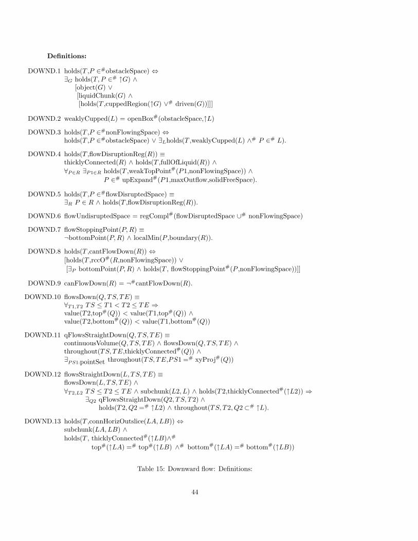
Definitions:

DOWND.1 holds(T ,P ∈#obstacleSpace) ⇔∃G holds(T, P ∈# ↑G) ∧

[object(G) ∨[liquidChunk(G) ∧[holds(T ,cuppedRegion(↑G) ∨# driven(G))]]]

DOWND.2 weaklyCupped(L) = openBox#(obstacleSpace,↑L)

DOWND.3 holds(T ,P ∈#nonFlowingSpace) ⇔holds(T ,P ∈#obstacleSpace) ∨ ∃Lholds(T ,weaklyCupped(L) ∧# P ∈# L).

DOWND.4 holds(T ,flowDisruptionReg(R)) ≡thicklyConnected(R) ∧ holds(T ,fullOfLiquid(R)) ∧∀P∈R ∃P1∈R holds(T ,weakTopPoint#(P1,nonFlowingSpace)) ∧

P ∈# upExpand#(P1,maxOutflow,solidFreeSpace).

DOWND.5 holds(T ,P ∈#flowDisruptedSpace) ≡∃R P ∈ R ∧ holds(T ,flowDisruptionReg(R)).

DOWND.6 flowUndisruptedSpace = regCompl#(flowDisruptedSpace ∪# nonFlowingSpace)

DOWND.7 flowStoppingPoint(P, R) ≡¬bottomPoint(P, R) ∧ localMin(P ,boundary(R)).

DOWND.8 holds(T ,cantFlowDown(R)) ⇔[holds(T ,rccO#(R,nonFlowingSpace)) ∨[∃P bottomPoint(P, R) ∧ holds(T , flowStoppingPoint#(P ,nonFlowingSpace))]]

DOWND.9 canFlowDown(R) = ¬#cantFlowDown(R).

DOWND.10 flowsDown(Q, TS, TE) ≡∀T1,T2 TS ≤ T 1 < T 2 ≤ TE ⇒value(T 2,top#(Q)) < value(T 1,top#(Q)) ∧value(T 2,bottom#(Q)) < value(T 1,bottom#(Q))

DOWND.11 qFlowsStraightDown(Q, TS, TE) ≡continuousVolume(Q, TS, TE) ∧ flowsDown(Q, TS, TE) ∧throughout(TS, TE,thicklyConnected#(Q)) ∧∃

PS1:pointSet throughout(TS, TE,PS1 =# xyProj#(Q))

DOWND.12 flowsStraightDown(L, TS, TE) ≡flowsDown(L, TS, TE) ∧∀T2,L2 TS ≤ T 2 ≤ TE ∧ subchunk(L2, L) ∧ holds(T 2,thicklyConnected#(↑L2)) ⇒

∃Q2 qFlowsStraightDown(Q2, TS, T 2) ∧holds(T 2, Q2 =# ↑L2) ∧ throughout(TS, T 2, Q2 ⊂# ↑L).

DOWND.13 holds(T ,connHorizOutslice(LA, LB)) ⇔subchunk(LA, LB) ∧holds(T , thicklyConnected#(↑LB)∧#

top#(↑LA) =# top#(↑LB) ∧# bottom#(↑LA) =# bottom#(↑LB))

Table 15: Downward flow: Definitions:

44

Axioms:

DOWN.1 maxOutflow > 0.

DOWN.2 liquidChunk(L) ∧throughout(TS, TE,slowObjectsInContact(↑L) ∧# canFlowDown(↑L)) ⇒flowsDown(↑L,TS, TE)

DOWN.3 liquidChunk(L) ∧ throughout(TS, TE,slowObjectsInContact(↑L)) ∧holds(TS, ↑L ⊂#flowUndisruptedSpace) ⇒∃TX,LX TS < TX ∧

holds(TS,connHorizOutslice(L, LX) ∧# rccDS#(↑LX ,nonFlowingSpace)) ∧flowsStraightDown(LX, TS, TX) ∧ holds(TX, rccC#(↑LX ,flowDisruptedSpace)).

DOWN.4 ∀TS,TE:time TS < TE ∧ bregion(R) ∧ distance(D) ∧ D > 0 ⇒

∃T1 TS < T 1 ≤ TE ∧∀

L:liquidChunk,T

TS ≤ T ≤ T 1 ∧ holds(T , ↑L ⊂#flowUndisruptedSpace ∧# ↑L ⊂# R) ⇒∃D1 hausdorff(value(T, ↑L),value(TS, ↑L),D1) ∧ D1 < D.

DOWN.5 ∀TS:time,R:bregion

[∀TE,RC TS ≤ TE ∧ RC ⊂ R ⇒noInflowDuring(R, TS, TE) ∧ ¬holds(TE,cuppedRegion(RC))]

⇒eventuallyForever(emptyLiquid(R)).

DOWN.6 liquidChunk(L) ∧ flowsDown(↑L, TS, TE) ∧ continuousVolume(QIN, TS, TE) ∧throughout(TS, TE,slowObjectMotion(OB) ∧# localMaxBox#(↑OB, QIN) ∧#

rccDS#(↑L,nonFlowingSpace)) ⇒value(TS, top#(QIN)) − value(TE, top#(QIN)) ≤

value(TS, top#(L)) − value(TE, top#(L)).

Table 16: Downward Flow: Axioms

45

��

��

RBRI1

RI2 DROPEN

Figure 16: Partial Box

PS.8 together with PD.8, PD.7, PD.6 asserts that from t0 to t1, the pitcher stays sufficientlyupright that the volume of the inside of the pitcher below the bottom of bTopPitcher is alwaysgreater than the volume of the liquid l0. This guarantees that bInsidePitcher does not overflowbetween t0 and t1.. (This is a sufficient condition, not a necessary one; the cupped region mayactually extend higher than the lowest point of bTopPitcher.)

PS.9 states that bSpout is a “spout” for oPitcher from time t1 onward. This is a geometricconstraint whose purpose is to guarantee that any overflow out of the pitcher to the outside mustpass through bSpout. The geometric definition is a little complicated. We say (PD.3) that RB is apartial box with true inside RI1, overflow region RI2, and opening ROPEN relative to the overflowdistance D if the following hold (figure 16):

• RB is a locally maximal box with inside RI1.

• The union of RB with ROPEN forms a open box with inside equal to RI2. RI2 containsRI1 and has a top D higher than the top of RI1.

RSPOUT is a spout for RB if

• RB is a partial box with opening ROPEN which is a subset of RSPOUT .

• RSPOUT ∪RB has no internal cavities other than the ones that are already in RB (RSPOUTis a bubble free attachment to RB (PD.1)).

PS.10 asserts that at t2, the maximal volume of any region cupped by oPitcher is less than thevolume of l0, so oPitcher must have overflowed before t2.

PS.15 states that oPail is motionless throughout the scenario. Therefore any geometric propertyof the pail that holds at t0 holds throughout the scenario.

PS.14 states that bInsidePail is the maximal open box formed by oPail. PS.13 states that thepart of bInsidePail that is at least maxOutflow below its top has a volume greater than l0. Thus,even if bInsidePail were filled with l0, the top of bInsidePail is still in freeFlowingSpace.

PS.16 states that from t1 onward the bottom of the spout is higher than the top of the pail.

PS.17 defines the fixed region “pouringRegion” as a vertical column rising from the inside ofbInsidePail and at least maxOuflow from the material of the pail (figure 17). The proof will workby showing that, once the liquid has been poured from the spout, it remains inside pouringRegion

PS.18 asserts that, from time t1 onward, the spout bSpout is always inside pouringRegion, morethan 2·maxOutflow from the boundaries of pouringRegion.

46

��

��

��

��

��

pouringRegion

Figure 17: Pouring region

PS.19 enforces the constraint that there are no channels on the outside of oPitcher that wouldallow liquid to flow from the inside of pouringRegion to within maxOutflow of the boundary ofpouringRegion. Otherwise, one could construct a scenario in which the liquid pours out of thespout, but is then caught by a channel on the exterior of the pitcher and guided to spill out at apoint that is not over the pail.

PS.20 and PS.21 enforce the “isolation” conditions that no objects other than the pitcher andthe pail and no liquids other than l0 interacts with the pouring of the liquid. PS.20 states that noobject other than oPitcher and no liquid other than l0 comes within 2·maxOutflow of the convexhull of oPitcher. PS.21 states that no objects other than oPitcher and oPail and no liquids otherthan l0 come within maxOutflow, horizontally, of the pouring region or of the inside of the pail. Inparticular, the pail is empty at t0 and no liquid other than l0 pours into the pail.

5.1 Correctness Proof

The proof of the desired inference from the axioms and the problem specification is very much assketched at the beginning of section 3. The detailed proof is rather long but not deep; it is given inthe online appendix at http://www.cs.nyu.edu/faculty/davise/papers/liqAppa.pdf.

The main steps are as follows (we enumerate only the most important axioms as justificationshere): By CUP.1, PS.10 the liquid remains in the pitcher as the pitcher is lifted into position. ByPS.12 at t2 the cupped volume in the pitcher is less than the volume of l0; hence using SPILL.1and SPILLD.5 the pitcher overflows at some point between t1 and t2. It follows from DOWN.2,DOWN.6 using a proof by contradiction that the liquid cannot rise more than maxOutflow abovethe region cupped by the pitcher. Hence, by PS.11, any liquid that flows out of the pitcher or out ofthe overflow region must go through the spout. By PS.12, PS.13, after t2 the cupped region in thepitcher is too small to hold the liquid; hence it must flow out of the pitcher. By PS.8 there is alwayssome cupped region inside the pitcher; hence by CUP.1 some of the liquid remains in the pitcher.By DOWN.2 the liquid in the overflow region must flow downward through the spout. When itflows out of the spout, by PS.20 it is inside pouringRegion. Using DOWN.2, DOWN.3, DOWN.4,PS.9, PS.21, PS.15 once the liquid is past the spout it remains inside pouringRegion until it is insidebInsidePail and at least maxOutflow below the top of the pail. (This is by far the hardest part ofthe proof; the proof is given in lemma 64 of the appendix). Once the liquid is inside the pail, thenby CUP.1, PS.10 it remains inside the pail. By DOWN.5 the part of pouringRegion above the pail

47

Symbols:

oPitcher, oPail → object.bInsidePitcher, bSpout, bTopPitcher → pseudo.l0 → liquidChunk.t0,t1,t2 → time.topSurface(PS:pointSet, R:region)partialBox(RB, RI1, RI2, ROPEN : bregion, D:distance)spout1(RB, RI1, RI2, RSPOUT, ROPEN :region,D:distance)spout(RSPOUT, RB:bregion, D;distance).pitcherShape(ROB, RIN :bregion, PTOP :pointSet ,RSPOUT :bregion).pitcher(OP :object, BI, BT, BS:pseudo) → fluent[Bool].volumeBelow(R:region, Z:ht) → volumepsBottom(PS:pointSet, Z:ht).simpleSafeTilt(BIN, BTOP : pseudo, V : volume)alwaysSimpleBox(RB: region)passOverBox(PASS:pointSet, RBOX, RIN :region)upColumn(PS:pointSet, Z:ht, PSC:pointSet).pouringRegion → fluent[region].simpleBox(R:region).convexHull(PS:pointSet) → pointSet.isolated(R:region, U :objectSet, L:liquidChunk) → fluent[Bool].maxBox(RB, RI:region).horizExpand(PS:pointSet, D:distance) → pointSet.

Table 17: Problem Specification: Symbols

and the overflow region above the pitcher are eventually empty. Hence eventually some of the liquidis in the pail, some of it is in the pitcher, and none of it is anywhere else.

5.2 Consistency Proof

Of course, the above inference is only significant if the problem specifications are consistent withthe domain axioms; if they are not, then one can prove anything at all. One can demonstrate thatthe specifications are consistent with the axioms by constructing a specific model of the shapes andmotions of the objects and the flow of the liquid that satisfies the specifications and axioms.

We sketch one such model below (figure 18). Assume a coordinate system where the z-axis isthe vertical and where the unit length is one inch.

Atemporal specifications:

Assume that maxOutflow = 2.

The inside of the pail is a 18 × 18 × 19 rectangular solid. The pail is a cubical box around theinside, open on top and with one inch walls on the sides and the bottom.

The pitcher is a 10 × 10 × 9 rectangular box, with the 8 × 8 × 8 block cut out from the centertop, and with a notch 2 inches deep cut out of the lower x-face. In other words: the bottom of thepitcher is 10 × 10 × 1. The lower x-side is 1 × 10 × 7 (this overlaps with the bottom). The upperx-side is 1 × 10 × 10, and the two y-faces are 10 × 1 × 10. The spout is the 1 × 8 × 2 notch cutout from the top of the lower x-face.

The volume of the liquid is 256 cubic inches.

48

Definitions:

PD.1 bubbleFreeAttachment(RA, RB) ≡rccEC(RA, RB) ∧¬∃R rccEC(R, RA) ∧ rccDS(R, RB) ∧boundary(R) ⊂ boundary(RA) ∪ boundary(RB) ∧¬[boundary(R) ⊂ boundary(RB)].

PD.2 topSurface(PS, R) ≡ ∀P P ∈ PS ⇔ topPoint(P, R).

PD.3 partialBox(RB, RI1, RI2, ROPEN, D) ≡localMaxBox(RB, RI1) ∧ RI1 ⊂ RI2 ∧ top(RI2)=top(RI1)+D ∧rccEC(RB, ROPEN) ∧ openBox(RB ∩ ROPEN, RI2,D)

PD.4 spout1(RB, RI1, RI2, RSPOUT, ROPEN, D) ≡partialBox(RB, RI1, RI2, ROPEN, D) ∧bubbleFreeAttachment(RSPOUT, RB) ∧ ROPEN ⊂ RSPOUT .

PD.5 spout(RSPOUT, RB, D) ≡∃RI1,RI2,ROPEN spout1(RB, RI1, RI2, RSPOUT, ROPEN, D).

PD.6 regionBelow(R, Z, RB) ≡∀

R1:region R1 ⊂ RB ⇔ R1 ⊂ R ∧ top(RB) ≤ Z.

PD.7 psBottom(PS, Z) ≡[∀P∈PS height(PS) ≥ Z] ∧[∀Z1 Z1 > Z ⇒ ∃P∈PS height(P ) < Z1].

PD.8 holds(T ,simpleSafeTilt(BIN, BTOP, V )) ≡∃Z,RB holds(T ,psBottom#(↑BTOP, Z) ∧# regionBelow#(↑BIN, Z, RB)) ∧V ≤volumeOf(RB)

PD.9 simpleBox(R) ≡∃R1 localMaxBox(R, R1) ∧

[∀R2 localMaxBox(R, R2) ⇒ R1 = R2] ∧[∀P flowStoppingPoint(P, R) ⇒ P ∈ R1].

PD.10 holds(T ,isolated(R, U, L)) ⇔∃

D:distance D > 0 ∧[∀

O:object holds(T ,dist#(↑O, R) <# D) ⇒ O ∈ U ] ∧[∀

L1:liquidChunk holds(T, ↑L1 ⊂# expand#(R, D)) ⇒ subchunk(L1, L)].

PD.11 maxBox(RB, RI) ≡openBox(RB, RI) ∧ [∀RC openBox(RB, RC) ∧ RI ⊂ RC ⇒ RI = RC].

PD.12 columnWithin(RC, RI) ≡∃RB,ZTOP RB ⊂ RI ∧ thicklyConnected(RB) ∧ upColumn(RB, ZTOP, RC)

PD.13 P ∈horizExpand(PS, D) ⇔∃PA∈PS dist(P, PS) ≤ D ∧ height(PA)=height(P ).

PD.14 onlyChannelsInReg(RB, RE, RX, ZTOP, D) ≡∀P weakTopPoint(P, RB) ∧ height(P ) ≤ ZTOP ∧ P ∈ RE ⇒

[P ∈ RX∨ horizExpand(P, D) ⊂ RE ∨ [∃RI openBox(RB, RI) ∧ P ∈ RI]]

Table 18: Problem Specification: Definitions

49

Axioms:

PS.1 t0 < t1 < t2

PS.2 oPitcher = source(bInsidePitcher) = source(bTopPitcher) = source(bSpout).

PS.3 holds(t0,openBox#(↑oPitcher,↑bInsidePitcher) ∧#

↑bTopPitcher =# topSurface#(↑bInsidePitcher))

PS.4 holds(t0,l0 ⊂# bInsidePitcher)

PS.5 foreverAfter(t0,slowObjectMotion(oPitcher)).

PS.6 ∀T t0≤ T ⇒∃H holds(T, psBottom#(↑bTopPitcher,H) ∧#

H ># bottom#(↑bInsidePitcher))

PS.7 foreverAfter(t0,simpleBox(oPitcher))

PS.8 throughout(t0,t1, simpleSafeTilt(bInsidePitcher,bTopPitcher,liqVolume(l0))).

PS.9 foreverAfter(t1,spout#(↑bSpout,↑oPitcher, maxOutflow)).

PS.10 ∃RI holds(t2, maxBox#(↑oPitcher,RI)) ∧ volumeOf(RI) < liqVolume(l0).

PS.11 foreverAfter(t2,motionless(oPitcher)).

PS.12 source(bInsidePail)=oPail.

PS.13 ∃R holds(t0,regionBelow#(↑bInsidePail, top#(↑bInsidePail)−#maxOutflow,R)) ∧volumeOf(R) > liqVolume(l0).

PS.14 holds(t0,maxBox#(↑oPail,↑bInsidePail) ∧# simpleBox(oPail))

PS.15 foreverAfter(t0,motionless(oPail)).

PS.16 foreverAfter(t1,top#(↑bInsidePail) <# bottom#(↑bSpout)).

PS.17 holds(t0,columnWithin#(pouringRegion,↑bInsidePail, topPouringRegion) ∧#

dist#(pouringRegion,↑oPail) ># maxOutflow)

PS.18 foreverAfter(t1,rccNTPP#(expand#(↑bSpout, 2·maxOutflow), pouringRegion))

PS.19 foreverAfter(t2,onlyChannelsInReg#(↑oPitcher, pouringRegion,↑bSpout,top#(↑bSpout),maxOutflow)

PS.20 foreverAfter(t0, isolated(expand#(convexHull#(↑oPitcher), 2·maxOutflow), { oPitcher }, l0))

PS.21 foreverAfter(t0, isolated(horizExpand#(pouringRegion ∪# ↑bInsidePail), maxOutflow){ oPail, oPitcher }, l0)).

Infer:

∃L1,L2:liquidChunk eventuallyForever(↑l0 =# ↑L1 ∪# ↑L2∧#

liqInContainer(L1,oPitcher) ∧# liqInContainer(L2,oPail)).

Table 19: Problem Specification: Axioms

50

��

��

��

��

��

��

��

��

��

��

��

��

��

��

��

��

Pail Pitcher

pouringRegion

Spout

TIme T0

After T2Time T2

Time T1

Figure 18: Model Scenario

51

shape(bInsidePail) = [1,19] × [1,19] × [1,20]

shape(oPail) = ([0,20] × [0,20] × [0,20]) − bInsidePail.

shape(bInsidePitcher) = [31,39] × [6,14] × [1,8].

shape(oPitcher) = ([30,40] × [5,15] × [0,9]) − (bInsidePitcher ∪ ([30,39] × [6,14] × [8,9]).

shape(bSpout) = [30,31] × [6,14] × [8,9]

liqVolume(l0) = 256.

pouringRegion = [4,15] × [5,15] × [4,43]

Time points: t0=0. t1=1. t2=2.

Initial State: At time t0, the pitcher and pail are at the positions specified by their shape.The liquid occupies the bottom half of the pitcher.

value(t0,placement(oPitcher)) = value(s0,placement(oPail)) = identity.

value(t0,place(l0)) = [31,39] × [6,14] × [1,5].

Motion of the rigid objects: The pail is motionless throughout. From t=0 to t=1/2, the pitchertranslates vertically 30 inches. From t=1/2 to t=1, the pitcher translates horizontally to the left 20inches. From t1 to t2 the pitcher rotates at a constant rate around the line x = 15, z = 35; this lineis parallel to the y-axis, sits at the top of the liquid, in the center of the x-extent of the top surfaceof the liquid. After t2 the pitcher is motionless.

motionless(oPail,j0)

0 ≤ T ≤ 1/2 ⇒ value(T ,placement(oPitcher)) = translate(0, 0, 60T )

1/2 ≤ T ≤ 1 ⇒ value(T ,placement(oPitcher)) = translate(−40(T − 1/2), 0, 30)

1 ≤ T ≤ 2 ⇒ value(T ,placement(oPitcher)) = rotateAroundAxis({〈15, Y, 35〉|real(Y )}, π(T − 1)/4)

(In the above formulas, the function “translate(X, Y, Z)” maps coordinates to a translation andthe function “rotateAroundAxis(PSL, A)” maps a line PSL and an angle A to a rotation in theobvious way.)

foreverAfter(t2,motionless(oPitcher)).

Liquid flow: There is no flow in the y-dimension. Hence, we will describe the flow purely in termsof its x-z component,

From t0 to t1 the liquid simply translates along with the pitcher.

The liquid flow from t1 to t2 is described as follows: Let Q2 be the region-valued fluent whosevalue is always the boxed region bounded by oPail ∪ bSpout. From t1 to t2, the liquid fills the sectionof that region which is below the plane z = 35. That is, we are supposing that the liquid flows inexactly the same way it would if the notch were filled in. Note that the volume of this sectionis constant; viewed in a coordinate system attached to the pitcher, this flow involves vacating atriangular wedge on the right and flowing into a congruent wedge on the left. Note that at t1, theliquid is simply observing rule 4 and in the region cupped by the pitcher. At some time tm beforet2, it reaches the edge of the pitcher and then starts to overflow. Between tm and t2 the liquid isfilling the maximal cupped region in the pitcher, and the volume of that region is monotonicallydecreasing; hence by SPILLD.5 the liquid is overflowing is overflowing out of the pitcher. Sinceit continues to overflow until t2, and since the specified region of overflow is all within the drivenarea, this pattern of flow is allowed by our rules. Within the region occupied by the liquid, theflow consists of a volume-preserving “rotation” around the axis of rotation. That is, as the pitcher

52

��

��

��

��

��

A: Liquid in state S2

Corner of pitcher

Spout

B: Flow lines out of overflow region

Oveflow region

Spout

Figure 19: Down flow from overflow region

rotates, every wedge of liquid centered at the axis replaces the wedge of equal volume to its left.

At t2, then, the liquid fills the cupped region bounded by oPitcher, plus a trapezoid over that(figure 19.A). After t2 the pitcher is motionless; hence, the volume of the maximal cupped region isconstant; hence, by SPILLD.5 the liquid is no longer considered to be overflowing, and is no longerdriven. The liquid in the cupped region remains where it is; the liquid in the overflow trapezoidmust all flow down. The liquid in the overflow trapezoid flows downward and to the left into thetriangle to the left of the overflow trapezoid, following the flow lines shown in figure 19.B. To seeintuitively that this can be done while maintaining constant volume, imagine cutting each flow tubeinto segments of equal volume, in a way that is consistent across the flow tubes. Then in each smalltime interval ∆T , each segment flows into the place vacated by the next segment in the tube.

Once the liquid has flowed out the bottom of the left hand triangle, it flows vertically in acolumn at a constant rate down toward the pail. Until the column hits the pail, it maintains itscolumnar shape. Once it has hit the bottom, there will be a rising pool occupying a cupped regionat the bottom of the pail. The part of the falling liquid more than maxOutflow above the top of thispool is in flowUndisruptedSpace and therefore continues to fall down in a column. The part of theliquid that is above the top of the pool but less than maxOutflow above it is in flowDisruptedSpace;it flows downward and outward, fast enough to make room for the column falling down after it.

It is an easy, but long and very uninteresting, exercise to specify this flow in closed formulas.

Verifying that the specified flow actually satisfies the axioms is not trivial, since some of the

53

axioms involve quantifying over all regions, or all region-valued fluents, but neither is it very difficult.

Of course, it would be undesirable to have to construct an explicit model like this for each newproblem specification, to make sure that the theory meaningfully applies to it. Much better wouldbe to have a general meta-theorem stating that all problem specifications of a specified form areconsistent with the axioms.

5.3 Other inferences

The above inference is the only one that I have worked through in full detail. However, I am quiteconfident that the following inferences are also justified in the theory. Moreover, their proof can usemany of the same general lemmas already worked through for our example.

• It is possible to ladle liquid out of a bowl with a spoon, if the spoon is immersed in the liquidand then lifted out, maintaining its cupped shape. The spoon may be immersed, either byplunging it in, so that the liquid spills over its side, or by sliding it in.

• If pebbles are gradually dropped into a vase filled with liquid, the level of the liquid willgradually rise. Once the volume of the pebbles plus the volume of the liquid exceeds thecapacity of the vase, the vase will overflow.

• If an object with no cups is immersed in a bowl of liquid and then lifted out, the removal ofthe object does not bring any liquid with it.

• If a large object is lowered gradually into a bowl of liquid, the liquid will reach the rim ofthe bowl just when the volume of the part of the object below the rim plus the volume of theliquid is equal to the capacity of the bowl. If part of the object is still above the liquid, thenlowering the object any further will cause the bowl to overflow.

• (Archimedes). Consider a scenario in which (1) object A is placed inside a bowl; (2) the bowlis filled to the brim with liquid; (3) object A is removed; (4) object B is placed inside the bowl.Assume that object A has no cups in which to carry out liquid. The bowl will overflow duringthe execution of (4) if and only if the volume of B is greater than the volume of A.

• If liquid is poured over a solid object suspended in the air, and the object does not form anycups then the liquid will flow down over the object, spreading a short distance beyond thebounds of the object. If the object does form cups then all of the liquid that is not caught inthose cups will pour down over the object in the same way.

• Suppose there is a body of liquid inside a simple cup with a plug at the bottom and the plugis removed. If there is nothing below the cup, then all the liquid will flow out the bottom. Ifthe cup is itself inside a bowl then the liquid will flow out the bottom of the cup into the bowluntil the level in the outer bowl is equal to the level in the cup.

• Suppose you have a W-shaped pail, and you pour from a pitcher into one of the internal cups(figure 20). The level of liquid will rise until it is full. Once it is full, the liquid will start topour off into the other internal cup. Once both internal cups are full, the two pools of liquidwill be joined on top, and the level will gradually rise across the entire pail.

54

��

��

��

��

Figure 20: Pouring into W-shaped Pail

��

��

maxOutflow

Cross section of channel:Steady state flow is only possible in the grey annulus.

The central core is all flowUndisruptedSpace.

Figure 21: Anomalous flow in channel

6 The Problem with Channels

The most immediate problem with our theory is that it completely mispredicts the way that waterflows in a channel. Not only does it fail to predict the correct behavior, it actually excludes thecorrect behavior. Suppose that there is a channel whose cross-section has a radius greater thanmaxOutflow filled with flowing water. The liquid chunks that are more than maxOutflow fromthe boundaries of the channel, in the center-top of the channel, are in flowUndisruptedSpace, andtherefore by rule 5 flow straight down rather than parallel to the channel. The only steady-state flowpattern allowed by rule 5 is one in which the water flows down in the annulus which is maxOutflowfrom the boundary of the channel (figure 21). This is all flowDisruptedSpace, and therefore theliquid there is allowed to flow parallel to the channel.

Thus, fixing this problem has two parts. The first part is to fix rule 5 so that it does not prohibitthe true flow down the channel; the second part is to add rules that require the correct flow. It iscertainly possible that the first part can be accomplished through some fairly minor change to rule 5that will eliminate this problem, while still preserving the ability to predict that liquid poured from

55

the pitcher lands in the pail. I doubt it, however; I suspect that even the first part of the solutionwill involve explicitly characterizing channels and marking them, like overflow, as an exception torule 5.

In any case, for the second part of the solution we need rules that will allow us to predict theflow of liquids in a channel. I intend to address this in future work. In the meantime, the problemprovides an interesting context for discussing the issues involved in extending a theory like this.Absent any great simplifying insight, adding channel flow to this theory will probably involve thefollowing:

• Defining a channel geometrically. This is considerably more challenging than defining a cup. Acup has a single distinguished direction – upward – which is fixed. A channel has two – upwardand forward – and the latter is defined relative to the channel and may change over the lengthof the channel. Also channels interact with each other and with other topographical featuresin more complicated ways than cups. Channels may split and merge; they may contain pits,bumps, and ridges.

• Defining the dynamics of “normal flow” in a channel. Again this is more complicated thanthe dynamics of cupped liquid; at its simplest, it is a steady-state flow rather than a staticcondition. For example, an open channel overflows its banks when the flow rate into thechannel exceeds the maximum flow rate that the channel can sustain; expressing this requiresa substantially richer theory than the simple rule for an overflowing cup. As with cups, wewould wish to at least partially categorize flow through a channel even in the case where thesolid object or objects forming the channel are in motion.

• Define the liquid in a channel as an exception to rule 5.

• Make sure that the rules accommodate the case of non-steady-state flow in a channel; forexample, a chunk of liquid falls onto the side of a channel. The prediction in a case like thisneed not be precise, but it should not be absurd, and it should smoothly interface with thenormal flow through a channel. For instance, if a chunk of liquid falls onto the side of a channelwhich has a channeled flow in it, the chunk should somehow merge with the channeled flow.

• Make sure that the examples that have been worked out still work. For instance the spout ofa pitcher may well be a channel, or it may not; make sure that the pitcher example works ineither case.

• As far as possible, check that the theory is still consistent.

Another problem is leaky cups. A cup with a small hole in fact works like a cup except fora slow leak, and can be used to carry liquid. But in our theory, a cup with a small hole is nota cup at all; the liquid inside can flow down (definition 3.4.4) and therefore must flow down (rule6). In particular, if the cup is lifted, our theory states that the liquid must flow out the hole fastenough that the absolute height of the top of the liquid always decreases. This problem, however,unlike the problem of channels is easy to fix; it is merely necessary to add a new rule similar torule 4 stating that leaky cups leak slowly, and to add the liquid cupped in a leaky cup as a part ofnonFlowingSpace in definition 3.4.2.

7 Conclusions and Future Work

We have constructed and formalized a theory that supports qualitative reasoning about many scenar-ios involving liquid flowing around slowly moving objects. There are a few scenarios that it handles

56

badly, but it seems likely that these can be corrected and that this theory can be an important partof a larger theory of commonsense physical reasoning.

The most important next steps in this research are:

• To develop a theory of liquid flow in channels.

• To develop a theory of liquid flow around rapidly moving objects.

• To integrate a theory of pressure, including atmospheric pressure.

• To integrate a theory of agents, with feedback from perception to manipulation, so that onecan describe the plan of carefully pouring liquid from a pitcher to a pail and reason about itsfeasibility.

• To define a reasonable subclass of inferences, particularly prediction, that can be effectivelyimplemented. The complexities of the proof in the appendix should not be discouraging,here; this is a complete proof based on very general axioms. If the language of the problemspecification and the closed-world assumptions can be standardized, and powerful generallemmas can be subsumed into procedures, then it may well be possible to develop an inferenceengine whose complexity is not much greater than the English description of the reasoninginvolved on page 3.1.

In the longer term, the critical problems are to identify significant classes of inference in this do-main, to develop effective algorithms for these, and to integrate these into knowledge-based systemsfor applications such as design, text interpretation, and automated tutoring.

References

[1] B. Bennett, A.G. Cohn. P. Torrini, and S.M. Hazarika, “Describing Rigid Body Motions in aQualitative Theory of Spatial Regions,” AAAI-00, pp. 503-509.

[2] A.G. Cohn and J. Renz, “Spatial Reasoning” in The Handbook of Knowledge Representation,F. van Harmelen, V. Lifschitz, and B. Porter (eds.), Elsevier, Oxford, 2007, to appear.

[3] J. Collins and K. Forbus, “Reasoning about Fluids via Molecular Collections,” AAAI-87,pp. 590-595.

[4] E. Davis, “A Logical Framework for Commonsense Predictions of Solid Object Behavior,” Int.Journal of AI in Engineering,, vol. 3, no. 3, 1988, pp. 125-140.

[5] E. Davis, Representations of Commonsense Reasoning, Morgan Kaufmann, 1990.

[6] E. Davis. “Axiomatizing Qualitative Process Theory,” KR-92, pp. 177-188.

[7] E. Davis, “The Kinematics of Cutting Solid Objects.” Annals of Mathematics and ArtificialIntelligence, Vol. 9, 1993, pp. 253-305.

[8] E. Davis, “The Naive Physics Perplex,” AI Magazine, Winter 1998, Vol. 19. No. 4. pp. 51-79.

[9] E. Davis, “Continuous Shape Transformations and Metrics on Regions,” Fundamenta Infor-maticae, Vol. 46, Nos. 1-2, 2001, pp. 31-54.

[10] E. Davis, “The Expressivity of Quantifying over Regions,” Journal of Logic and Computation,vol. 16, 2006, pp. 891-916.

57

[11] E. Davis, “How Does a Box Work? A Study in the Qualitative Dynamics of Solid Objects.”Submitted to Artificial Intelligence, 2007.

[12] E. Davis, The Logic of Commonsense Physical Reasoning, in preparation.

[13] J. DeCuyper, D. Keymeulen, and L. Steels, “A Hybrid Architecture for Modelling Liquid Behav-ior,” in J. Glasgow, B. Chandrasekaran, and N.H. Narayanan (eds.) Diagrammatic Reasoning,MIT Press, 1995, pp. 731-751.

[14] J. de Kleer, “Multiple Representations of Knowledge in a Mechanics Problem Solver” IJCAI-77,pp. 299-304.

[15] J. de Kleer and J.S. Brown, “A Qualitative Physics Based on Confluences.” In D. Bobrow (ed.)Qualitative Reasoning about Physical Systems. Cambridge, Mass.: MIT Press, 1985, pp. 7-83.

[16] K. Forbus, “Qualitative Process Theory”, In Bobrow, D. (ed.) Qualitative Reasoning aboutPhysical Systems, Cambridge, Mass.: MIT Press, 1985, pp. 85-186.

[17] F. Gardin and B. Meltzer, “Analogical Representations of Naive Physics,” in J. Glasgow,B. Chandrasekaran, and N.H. Narayanan (eds.) Diagrammatic Reasoning, MIT Press, 1995,pp. 669-689.

[18] P. Hayes, “The Naive Physics Manifesto,” in D. Michie (ed.) Expert Systems in the Microelec-tronic Age. Edinburgh: Edinburgh University Press, 1979.

[19] P. Hayes, “Ontology for Liquids,” in J. Hobbs and R. Moore (eds.) Formal Theories of theCommonsense World, Norwood NJ, Ablex Pub., 1985.

[20] P. Hayes, “A Critique of Pure Treason”, Computational Intelligence, vol. 3, 1987, pp. 179-185.

[21] H. Kim, Qualitative Reasoning about Fluids and Mechanics, Ph.D. thesis, Institute of LearningSciences, Northwestern University, 1993.

[22] L. Joskowicz and E. Sacks, “Computational Kinematics,” Artificial Intelligence, vol. 51, 1991,pp. 381-416.

[23] V. Lifschitz, “Cracking an Egg: An Exercise in Formalizing Commonsense Reasoning,” FourthSymposium on Logical Formalizations of Commonsense Reasoning, 1998.

[24] J. McCarthy, “Programs with common sense,” in: M. Minsky (ed.) Semantic InformationProcessing, MIT Press, Cambridge, MA, 1968, pp. 403-418.

[25] J. McCarthy and P. Hayes, “Some Philosophical Problems from the Standpoint of ArtificialIntelligence,” in B. Meltzer and D. Michie (eds.) Machine Intelligence 4, Edinburgh UniversityPress, 1969.

[26] D. McDermott, “A Critique of Pure Reason”, Computational Intelligence, vol. 3, 1987, pp.151-160.

[27] L. Morgenstern. “Mid-Sized Axiomatizations of Commonsense Problems: A Case Study in EggCracking,” Studia Logica, vol. 67, 2001, pp. 333-384.

[28] A. Newell, “The Knowledge Level,” AI Magazine, vol. 2 no. 2, 1981.

[29] D.A. Randell, Z. Cui, and A.G. Cohn, “A spatial logic based on regions and connection,”Third International Conference on Principles of Knowledge Representation and Reasoning,1992, pp. 165-176.

58

[30] R. Reiter, Knowledge in Action: Logical Foundations for Specifying and Implementing Dynam-ical Systems, MIT Press, Cambridge, MA, 2001.

[31] E. Sandewall, “Combining Logic and Differential Equations for Describing Real-World Sys-tems,” KR-89, pp. 412-420.

[32] J. Schmolze, “Physics for Robots,” AAAI-86, pp. 44-50.

[33] M. Shanahan. “An Attempt to Formalise a Non-Trivial Problem in Common Sense Reasoning,”Artificial Intelligence, Vol. 153, 2004, pp. 141-165.

[34] J. Shin and E. Davis, “Processes and Continuous Change in a SAT-Based Planner,” ArtificialIntelligence, vol. 166 nos. 1-2, 2005, pp. 194-253.

59

Documents

Pouring Liquids: A Study in Commonsense Physical Reasoning · PDF filefrom one container to another, ... and demonstrates that this inference and other similar inferences can be