Embed Size (px)
Citation preview

Power and Sample Size Calculation for
Log-rank Test under a Non-proportional
Hazards Model∗
Daowen Zhang
Department of Statistics
North Carolina State University
http://www4.stat.ncsu.edu/∼dzhang2/
∗ Joint work with Hui Quan, Department of Biostatistics &
Programming, Sanofi-Aventis
1

OUTLINE
1. Motivating example: Rimonabant trial on cardiovascular
risk
2. Review of the log-rank test statistic
3. Distributions of the log-rank test statistic
4. Detailed power calculation
5. Example and simulation Results
6. Summary
2

1. Motivating example: Rimonabant trial
• Rimonabant trial: Assess the benefit of Rimonabant on reducing
cardiovascular risk.
• Placebo-controlled
• Primary endpoint: time to cardiovascular event; event rates
expected to be low in each group
• Log-rank test was proposed to assess the treatment effect.
• Power and sample size consideration should also be based on the
log-rank test
3

• It is straightforward if treatment effect is characterized by
λ1(t)
λ0(t)= eβ ,
λ1(t): hazard of cardiovascular event for treatment
λ0(t): hazard of cardiovascular event for placebo
• If β ≈ 0 and censoring process independent of treatment group,
log-rank test statistic T has distribution (Schoenfeld, 1981
Biometrika)
Ta∼ N(β
√θ(1 − θ)D, 1),
θ: Allocation probability to the treatment
D: Expected total # of deaths (under Ha) from both groups
4

• Can be used to calculate power and sample size if the treatment
effect model (PH model) is reasonable.
• However ...
5

6

• Other issues:
1. censoring (information cannot be retrieved)
2. drop-out (information can be retrieved during the study)
• How to handle drop-out?
1. treat it as censoring: assumption?
2. conduct ITT analysis: efficiency loss?
• Problem: how to calculate power and sample size for each
strategy? which is better?
• Need to investigate the distribution of the log-rank test statistic
for our problem
7

2. Review of the log-rank test statistic
• The (standard) log-rank test statistic
T =U√
v̂ar(U),
where
U =∑
x
{d1(x) − n1(x)
d(x)
n(x)
}
v̂ar(U) =∑
x
n1(x)n0(x)d(x){n(x) − d(x)}n2(x){n(x) − 1}
8

• Under H0 : S1(t) = S0(t) ⇐⇒ H0 : λ1(t) = λ0(t),
Ta∼ N(0, 1)
So reject H0 if |T | ≥ zα/2.
• Under Ha : λ1(t) 6= λ0(t) (but λ1(t) ≈ λ0(t)) (Schoenfeld, 1981
Biometrika)
Ta∼ N(φ, 1),
where
φ =
√n
∫ ∞
0log{λ1(t)/λ0(t)}π(t){1 − π(t)}V (t)dt
[∫ ∞
0π(t){1 − π(t)}V (t)dt]1/2
,
where V (t) describes process of observing deaths, π(t) −→ θ if
censoring process is the same in both groups.
9

• Special case: PH alternative
Ha :λ1(t)
λ0(t)= eβ (β ≈ 0),
then
Ta∼ N(β
√θ(1 − θ)D, 1),
• Can be used to calculate the power for PH alterative.
10
3. Distribution of the log-rank test statistic
• It is reasonable to assume the alternative for our problem:
Ha :λ1(t)
λ0(t)=
1 t ∈ [0, t0)
eβ (β ≈ 0) t ∈ [t0,∞)
λ1(t) = hazard of treated group
λ0(t) = hazard of untreated group
• Distributions of the log-rank test statistic under Ha for two
strategies?
1. Strategy 1: Treat drop-out as censoring
2. Strategy 2: Conduct ITT analysis
11

Distribution for Strategy 1
• Direct use of the result of Schoenfeld, 1981 (Biometrika) =⇒
Ta∼ N(φ, 1),
φ ≈√
nβ∫ ∞
t0π(t){1 − π(t)}V (t)dt
[∫ ∞
0π(t){1 − π(t)}V (t)dt]1/2
≈ β√
θ(1 − θ) × D̃√D
,
D = total expected # of deaths from two groups in the study
D̃ = total expected # of deaths from two groups after t0.
• Power = P [Z > |φ| − zα/2].
• Concern: approximation good enough? better one?
12

• The use of a series of double expectation theorem leads to
φ ≈√
θ(1 − θ) × (1 − e−β)D̃1 + (eβ − 1)D̃0√D
D̃1 = total # of deaths from treated group after t0D̃0 = total # of deaths from untreated group after t0
• Assumption: drop-out independent of the (unerlying) survival
time had the patient not dropped out; the same in both groups.
• Let
D1 = total expected # of deaths from treated group
D0 = total expected # of deaths from untreated group
D∗1 = total expected # of deaths from treated group before t0
D∗0 = total expected # of deaths from placebo group before t0
D = D0 + D1, D̃1 = D1 − D∗1, D̃0 = D0 − D∗
0
13
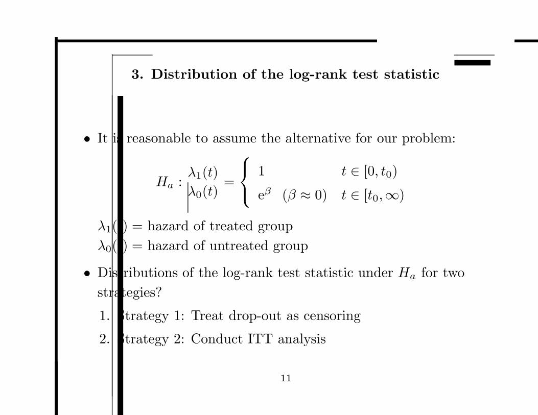
Distribution for Strategy 2
• Lakatos (1988, Biometrics) derived an approx. dist. of the
log-rank test under any Ha : λ∗1(t) 6= λ∗
0(t) (λ∗1(t) ≈ λ∗
0(t)).
• λ∗0(t) = hazard of the group randomized to placebo
λ∗1(t) = hazard of the group randomized to treatment
• Partition patient time [0, L = A + F ) = ∪[ti, ti+1) with equal
width ∆.
0
-
ti ti+1 F L = A + F
A = accrual period, F = follow-up time, L = study length.
14

• Under Ha : λ∗1(t) 6= λ∗
0(t) (λ∗1(t) ≈ λ∗
0(t)):
Ta∼ N(φ, 1),
φ ≈∑
Di
{ξipi
1+ξipi
− pi
1+pi
}
{∑Di
pi
(1+pi)2
}1/2
1. Di = {n1(ti)λ∗1(ti) + n0(ti)λ
∗0(ti)}∆
= total expected # of deaths in [ti, ti+1)
2. ξi = λ∗1(ti)/λ
∗0(ti)
3. pi = n1(ti)/n0(ti)
15

4. n0(ti), n1(ti), number of patients at risk, can be calculated
iteratively:
nk(ti+1) =
nk(ti){1 − λ∗k(ti)∆} ti < F
nk(ti){
1 − λ∗k(ti)∆ − ∆
L−ti
}ti ≥ F
Assume constant accrual rate in [0, A].
• Need to know the hazard function for each (randomized) group.
16
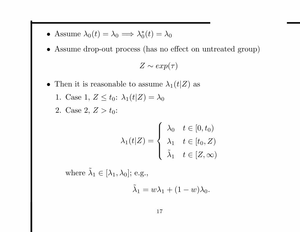
• Assume λ0(t) = λ0 =⇒ λ∗0(t) = λ0
• Assume drop-out process (has no effect on untreated group)
Z ∼ exp(τ)
• Then it is reasonable to assume λ1(t|Z) as
1. Case 1, Z ≤ t0: λ1(t|Z) = λ0
2. Case 2, Z > t0:
λ1(t|Z) =
λ0 t ∈ [0, t0)
λ1 t ∈ [t0, Z)
λ̃1 t ∈ [Z,∞)
where λ̃1 ∈ [λ1, λ0]; e.g.,
λ̃1 = wλ1 + (1 − w)λ0.
17

• The survival function for group randomized to treatment:
S∗1(t) = E{I(T ≥ t)}
= E[E{I(T ≥ t)|Z}]= E{S1(t|Z)}.
• Case 1, Z < t0:
S1(t|Z) = e−λ0t
• Case 2: Z ≥ t0:
S1(t|Z) = e−Λ1(t|Z) =
e−λ0t t ∈ [0, t0)
e−λ0t0−λ1(t−t0) t ∈ [t0, Z)
e−λ0t0−λ1(Z−t0)−λ̃1(t−Z) t ∈ [Z,∞)
18

• Can calculate S∗1(t) and f∗
1 (t) and hence
λ∗1(t) =
f∗1 (t)
S∗1(t)
.
• Then can calculate the nc φ in N(φ, 1) for the log-rank test.
• For better numerical accuracy, ∆ needs to be small, say, 1/1000,
if unit = year.
19

4. Detailed power calculation for strategy 1
• Some assumptions:
1. Other than drop-out, end-of-study is the only other censoring
(can be relaxed)
2. [0, A) is the accrual period, a = accrual rate (can be a(t))
3. F = follow-up period, L = A + F = total study length
4. F ≥ t0.
5. λ0(t) = λ0.
20

• Consider [t, t + dt) in [0, A):
0
-
t t + dt A L
• Average # of patients entering into study in [t, t + dt):
θadt treatment group
(1 − θ)adt placebo group(1)
21

• The probability that a patient entering at t is observed to die in
the study (i.e., dies before L) is
P [T ≤ min(L − t, Z)]
• The probability that a patient entering at t is observed to die
before t0 is
P [T ≤ min(t0, Z)]
22

• For placebo group:
P [T ≤ min(L − t, Z)] = E[E{I[T ≤ min(L − t, Z)]|Z}]
The inner expectation can be shown to be
E{I[T ≤ min(L − t, Z)]|Z} =
1 − e−λ0(L−t) Z ≥ L − t
1 − e−λ0Z Z < L − t
=⇒
P [T ≤ min(L − t, Z)] =λ0
λ0 + τ− λ0
λ0 + τe−(λ0+τ)(L−t)
23

• The total expected # of deaths in the study for placebo group:
D0 =
∫ A
0
a(1 − θ)P [T ≤ min(L − t, Z)]dt
=a(1 − θ)λ0
λ0 + τ
[A − e−(λ0+τ)L
λ0 + τ{e(λ0+τ)A − 1}
].
• The total expected # of deaths for placebo group before t0:
D∗0 =
∫ A
0
a(1 − θ)P [T ≤ min(t0, Z)]dt
=aA(1 − θ)λ0
λ0 + τ{1 − e−(λ0+τ)t0}.
24
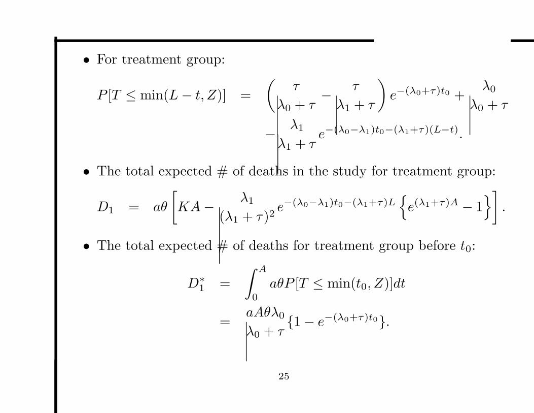
• For treatment group:
P [T ≤ min(L − t, Z)] =
(τ
λ0 + τ− τ
λ1 + τ
)e−(λ0+τ)t0 +
λ0
λ0 + τ
− λ1
λ1 + τe−(λ0−λ1)t0−(λ1+τ)(L−t).
• The total expected # of deaths in the study for treatment group:
D1 = aθ
[KA − λ1
(λ1 + τ)2e−(λ0−λ1)t0−(λ1+τ)L
{e(λ1+τ)A − 1
}].
• The total expected # of deaths for treatment group before t0:
D∗1 =
∫ A
0
aθP [T ≤ min(t0, Z)]dt
=aAθλ0
λ0 + τ{1 − e−(λ0+τ)t0}.
25

5. Example and simulation results
• Expect new treatment takes effect after 1 year =⇒ t0 = 1
• Rate to have cardiovascular risk 0.03 per year (λ0 = 0.03)
• Expect 25% reduction when new treatments takes its full effect
(λ1 = 0.0225).
• Accrual rate a = 1000 patients/month
• Study length (L = 50) months
• Expect 10% (per year) drop-out rate
• Significance level α = 0.05; targeted power = 0.9
• How long should the accrual period (A) be? And sample size?
26

1.0 1.2 1.4 1.6 1.8 2.0
0.85
0.90
0.95
Accrual period in years
Powe
r
Solution 1: 1.313 years
solution 2: 1.385 years
accrual rate: 12000 patients/yearstudy length: 4.17 years
27
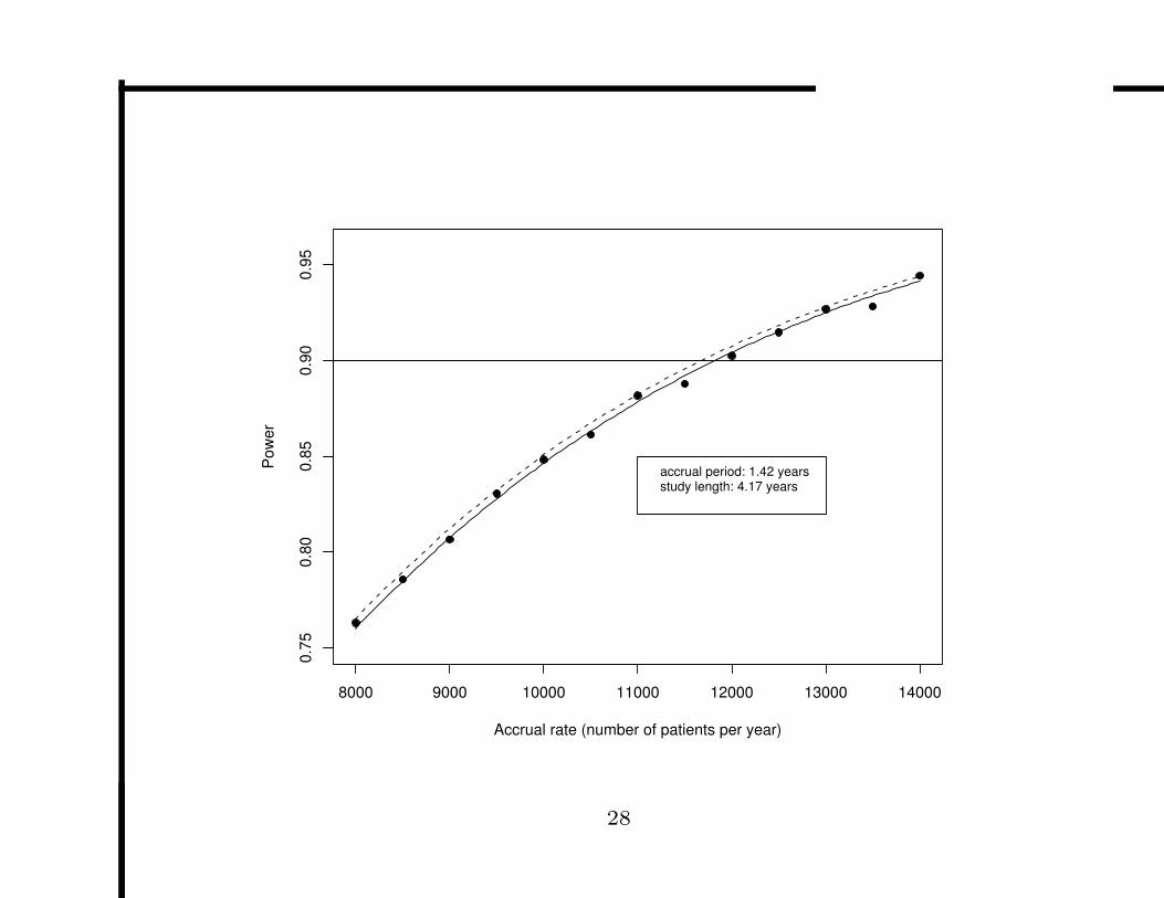
8000 9000 10000 11000 12000 13000 14000
0.75
0.80
0.85
0.90
0.95
Accrual rate (number of patients per year)
Powe
r
accrual period: 1.42 yearsstudy length: 4.17 years
28

3.6 3.8 4.0 4.2 4.4
0.75
0.80
0.85
0.90
0.95
Study length in years
Powe
r
accrual rate: 12000 patients/yearaccrual period: 1.42 years
29
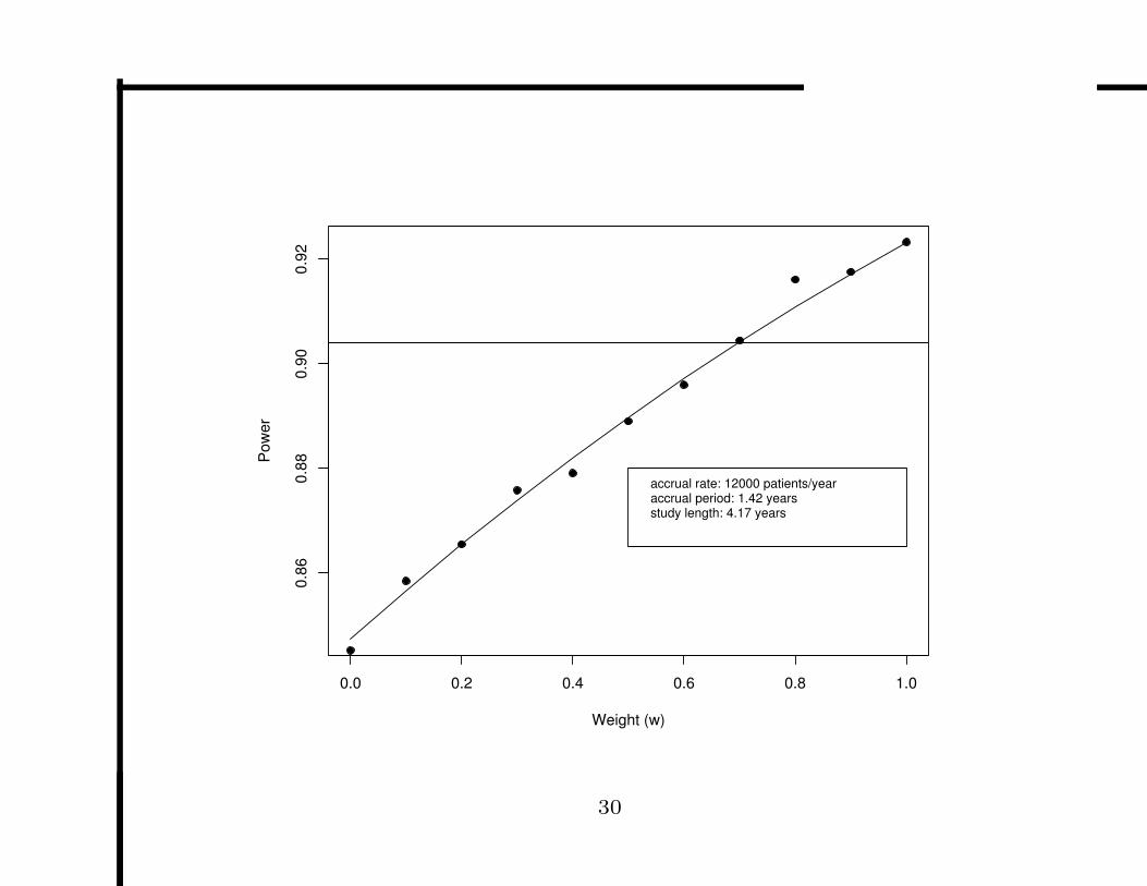
0.0 0.2 0.4 0.6 0.8 1.0
0.86
0.88
0.90
0.92
Weight (w)
Powe
r
accrual rate: 12000 patients/yearaccrual period: 1.42 yearsstudy length: 4.17 years
30

1.0 1.2 1.4 1.6 1.8 2.0
0.70
0.75
0.80
0.85
0.90
0.95
Accrual period in years
Powe
r
accrual rate: 12000 patients/yearstudy length: 4.17 years
31

8000 9000 10000 11000 12000 13000 14000
0.70
0.75
0.80
0.85
0.90
0.95
Accrual Rate (number of patients per year)
Powe
r
accrual period: 17 monthsstudy length: 50 months
32

3.6 3.8 4.0 4.2 4.4
0.70
0.75
0.80
0.85
0.90
0.95
Study Length in Year
Powe
r
accrual rate: 12000 patients/yearaccrual period: 17 months
33

software: S-plus function logrankpower(
alpha=0.05, signifance level of the log-rank test
lambda0=, hazard for placebo
lambda1=, hazard for treatment
t0=0, t0 used in the formula
wt=0.5, weight for residual treatment effect
tau=0, drop-out rate
acrate=, accrual rate
acperiod=, accrual period
slength=, study lenght (slength-acperiod>t0)
theta=0.5, allocation prob
nsub=1000, number of sub-intervals for ITT analysis
itt=F flag for ITT analysis)
34

6. Discussion
• Delayed treatment effect + drop-outs present challenge to
statisticians
• Proposed two strategies:
1. Treat drop-outs as censored observations
(a) Assumption: drop-out process independent of (underlying
true) time to event
(b) Drop-out processes almost the same in both groups.
(c) Calculation straightforward
(d) Don’t need to specify the hazard for untreated group
2. Conduct ITT analysis:
(a) May be what regulatory agencies want
(b) May have enough power only if residual treatment effect is
35

relatively large (70% in our example)
(c) Can be computationally intensive (small ∆)
(d) Have to specify the hazard for untreated group
• Derived formula easy to use; confirmed by simulation to have
good statistical properties
• Can include other censoring
36