Embed Size (px)
Citation preview

Power grid vulnerability analysis
Daniel Bienstock
Columbia University
Dimacs 2010
Daniel Bienstock (Columbia University) Power grid vulnerability analysis Dimacs 2010 1 / 45
Background: a power grid is three systems
DISTRIBUTION
GENERATION
TRANSMISSION
Daniel Bienstock (Columbia University) Power grid vulnerability analysis Dimacs 2010 2 / 45

Challenges to analysis
Power grids follow the laws of physics, characterized by nonlinear,nonconvex equations that make fast computation difficult.
Furthermore, direct control is difficult: we cannot dictate howpower will flow.
Power grids are subject to “noise” which is difficult to modelaccurately.
Power grids can exhibit non-monotone behavior as a result ofcontrol or adversarial actions.
Power grids can cascade.
Daniel Bienstock (Columbia University) Power grid vulnerability analysis Dimacs 2010 3 / 45
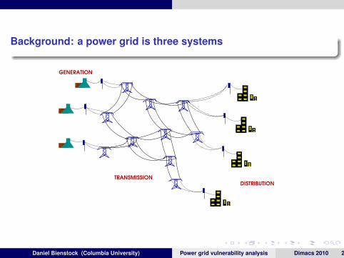
AC power flows – polar coordinates
→ Voltage at a node (“bus”) k is of the form Uk ejθk , where j =√
−1
→ Power flowing on edge (“line”) {k , m} equals pkm + jqkm, where
pkm = U2k gkm − Uk Um gkm cos θkm − Uk Um bkm sin θkm
qkm = −U2k (bkm + bsh
km) + Uk Um bkm cos θkm − Uk Um gkm sin θkm
Here, θkm.= θk − θm
gkm, bkm, bshkm are known parameters (series conductance, series reactance,
shunt susceptance)
Daniel Bienstock (Columbia University) Power grid vulnerability analysis Dimacs 2010 4 / 45

Voltage at k = Uk ejθk ; power on line {k , m} = pkm + jqkm, where
pkm = U2k gkm − Uk Um gkm cos θkm − Uk Um bkm sin θkm
qkm = −U2k (bkm + bsh
km) + Uk Um bkm cos θkm − Uk Um gkm sin θkm
( θkm.= θk − θm)
Pk = Σ{k ,m}pkm (active power), Qk = Σ{k ,m}qkm (reactive power)
Power flow problem: Choose the vectors p, q, θ, P, Q so as to satisfy allequations above, and
meet demand requirements and generator constraints
and, ideally, meet thermal constraints (flow limits) on the power lines
Daniel Bienstock (Columbia University) Power grid vulnerability analysis Dimacs 2010 5 / 45
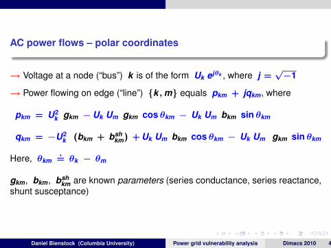
Research challenges
→ Do we have fast and reliable algorithm for the power flow problem?
Should not require human input in order to terminate.
When no “acceptable” solution exists, should produce a certificatethat this is the case.
What about the cases where multiple solutions exist?
After a contingency has take place, or a control has been applied:which solution should be instantiated?
What if all solutions are “bad”?
Daniel Bienstock (Columbia University) Power grid vulnerability analysis Dimacs 2010 6 / 45

Solution methodologies
Newton-Raphson (iterative) algorithms to solve system ofequations
The claim: this “always” works fast. At least in the case of a“normal” system.
New result: Low et al (2010). Some (many?) optimal power flowproblems can be solved using semidefinite programming.
Daniel Bienstock (Columbia University) Power grid vulnerability analysis Dimacs 2010 7 / 45

Solution methodologies
Newton-Raphson (iterative) algorithms to solve system ofequations
The claim: this “always” works fast.
At least in the case of a“normal” system.
New result: Low et al (2010). Some (many?) optimal power flowproblems can be solved using semidefinite programming.
Daniel Bienstock (Columbia University) Power grid vulnerability analysis Dimacs 2010 7 / 45

Solution methodologies
Newton-Raphson (iterative) algorithms to solve system ofequations
The claim: this “always” works fast. At least in the case of a“normal” system.
New result: Low et al (2010). Some (many?) optimal power flowproblems can be solved using semidefinite programming.
Daniel Bienstock (Columbia University) Power grid vulnerability analysis Dimacs 2010 7 / 45

Solution methodologies
Newton-Raphson (iterative) algorithms to solve system ofequations
The claim: this “always” works fast. At least in the case of a“normal” system.
New result: Low et al (2010). Some (many?) optimal power flowproblems can be solved using semidefinite programming.
Daniel Bienstock (Columbia University) Power grid vulnerability analysis Dimacs 2010 7 / 45
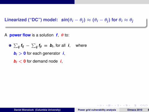
Linearized (“DC”) model: sin(θi − θj) ≈ (θi − θj) for θi ≈ θj
A power flow is a solution f , θ to:∑ij fij −
∑ij fji = bi , for all i , where
bi > 0 for each generator i ,
bi < 0 for demand node i ,
xij fij − θi + θj = 0 for all (i, j). ( xij = “reactance”)
Lemma: Given a choice for b with∑
i bi = 0 (a requirement),the system has a unique (in f) solution.
Daniel Bienstock (Columbia University) Power grid vulnerability analysis Dimacs 2010 8 / 45

Linearized (“DC”) model: sin(θi − θj) ≈ (θi − θj) for θi ≈ θj
A power flow is a solution f , θ to:∑ij fij −
∑ij fji = bi , for all i , where
bi > 0 for each generator i ,
bi < 0 for demand node i ,
xij fij − θi + θj = 0 for all (i, j). ( xij = “reactance”)
Lemma: Given a choice for b with∑
i bi = 0 (a requirement),
the system has a unique (in f) solution.
Daniel Bienstock (Columbia University) Power grid vulnerability analysis Dimacs 2010 8 / 45

Linearized (“DC”) model: sin(θi − θj) ≈ (θi − θj) for θi ≈ θj
A power flow is a solution f , θ to:∑ij fij −
∑ij fji = bi , for all i , where
bi > 0 for each generator i ,
bi < 0 for demand node i ,
xij fij − θi + θj = 0 for all (i, j). ( xij = “reactance”)
Lemma: Given a choice for b with∑
i bi = 0 (a requirement),the system has a unique (in f) solution.
Daniel Bienstock (Columbia University) Power grid vulnerability analysis Dimacs 2010 8 / 45
A quote from:
Final Report on the August 14, 2003 Blackout in the United Statesand Canada: Causes and Recommendations, U.S.-Canada PowerSystem Outage Task Force, April 5, 2004. (https://reports.energy.gov)
Cause 1 was “inadequate system understanding” – stated 20 times
Cause 2 was “inadequate situational awareness” – stated 14 times
Cause 3 was “inadequate tree trimming” – stated 4 times
Cause 4 was “inadequate RC diagnostic support” – stated 5 times
Daniel Bienstock (Columbia University) Power grid vulnerability analysis Dimacs 2010 9 / 45

A quote from:
Final Report on the August 14, 2003 Blackout in the United Statesand Canada: Causes and Recommendations, U.S.-Canada PowerSystem Outage Task Force, April 5, 2004. (https://reports.energy.gov)
Cause 1 was “inadequate system understanding”
– stated 20 times
Cause 2 was “inadequate situational awareness” – stated 14 times
Cause 3 was “inadequate tree trimming” – stated 4 times
Cause 4 was “inadequate RC diagnostic support” – stated 5 times
Daniel Bienstock (Columbia University) Power grid vulnerability analysis Dimacs 2010 9 / 45

A quote from:
Final Report on the August 14, 2003 Blackout in the United Statesand Canada: Causes and Recommendations, U.S.-Canada PowerSystem Outage Task Force, April 5, 2004. (https://reports.energy.gov)
Cause 1 was “inadequate system understanding” – stated 20 times
Cause 2 was “inadequate situational awareness” – stated 14 times
Cause 3 was “inadequate tree trimming” – stated 4 times
Cause 4 was “inadequate RC diagnostic support” – stated 5 times
Daniel Bienstock (Columbia University) Power grid vulnerability analysis Dimacs 2010 9 / 45

A quote from:
Final Report on the August 14, 2003 Blackout in the United Statesand Canada: Causes and Recommendations, U.S.-Canada PowerSystem Outage Task Force, April 5, 2004. (https://reports.energy.gov)
Cause 1 was “inadequate system understanding” – stated 20 times
Cause 2 was “inadequate situational awareness” – stated 14 times
Cause 3 was “inadequate tree trimming” – stated 4 times
Cause 4 was “inadequate RC diagnostic support” – stated 5 times
Daniel Bienstock (Columbia University) Power grid vulnerability analysis Dimacs 2010 9 / 45
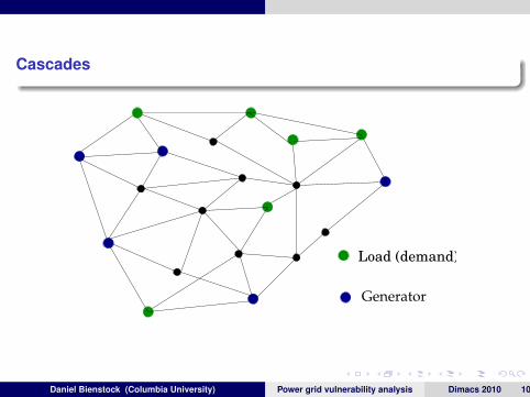
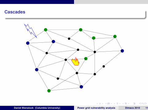
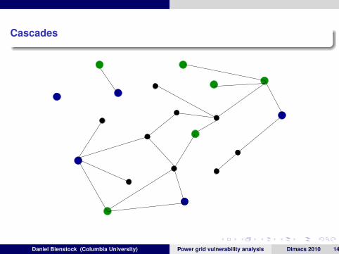
Cascades
Generator
Load (demand)
Daniel Bienstock (Columbia University) Power grid vulnerability analysis Dimacs 2010 10 / 45
Cascades
Daniel Bienstock (Columbia University) Power grid vulnerability analysis Dimacs 2010 11 / 45

Cascades
Daniel Bienstock (Columbia University) Power grid vulnerability analysis Dimacs 2010 12 / 45

Cascades
Daniel Bienstock (Columbia University) Power grid vulnerability analysis Dimacs 2010 13 / 45
Cascades
Daniel Bienstock (Columbia University) Power grid vulnerability analysis Dimacs 2010 14 / 45

Cascades
= lost demand
Daniel Bienstock (Columbia University) Power grid vulnerability analysis Dimacs 2010 15 / 45

Cascades
Daniel Bienstock (Columbia University) Power grid vulnerability analysis Dimacs 2010 16 / 45

Cascades
Daniel Bienstock (Columbia University) Power grid vulnerability analysis Dimacs 2010 17 / 45
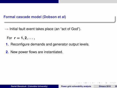
Formal cascade model (Dobson et al)
→ Initial fault event takes place (an “act of God”).
For r = 1, 2, . . . ,
1. Reconfigure demands and generator output levels.
Daniel Bienstock (Columbia University) Power grid vulnerability analysis Dimacs 2010 18 / 45
Formal cascade model (Dobson et al)
→ Initial fault event takes place (an “act of God”).
For r = 1, 2, . . . ,
1. Reconfigure demands and generator output levels.
Daniel Bienstock (Columbia University) Power grid vulnerability analysis Dimacs 2010 18 / 45

Islanding
supply > demand
Daniel Bienstock (Columbia University) Power grid vulnerability analysis Dimacs 2010 19 / 45
Formal cascade model (Dobson et al)
→ Initial fault event takes place (an “act of God”).
For r = 1, 2, . . . ,
1. Reconfigure demands and generator output levels.
2. New power flows are instantiated.
3. The next set of faults takes place.(Stochastic or history-dependent criterion)
Daniel Bienstock (Columbia University) Power grid vulnerability analysis Dimacs 2010 20 / 45

Formal cascade model (Dobson et al)
→ Initial fault event takes place (an “act of God”).
For r = 1, 2, . . . ,
1. Reconfigure demands and generator output levels.
2. New power flows are instantiated.
3. The next set of faults takes place.
(Stochastic or history-dependent criterion)
Daniel Bienstock (Columbia University) Power grid vulnerability analysis Dimacs 2010 20 / 45

Formal cascade model (Dobson et al)
→ Initial fault event takes place (an “act of God”).
For r = 1, 2, . . . ,
1. Reconfigure demands and generator output levels.
2. New power flows are instantiated.
3. The next set of faults takes place.(Stochastic or history-dependent criterion)
Daniel Bienstock (Columbia University) Power grid vulnerability analysis Dimacs 2010 20 / 45
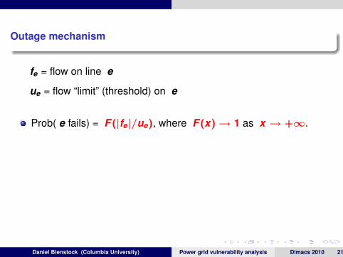
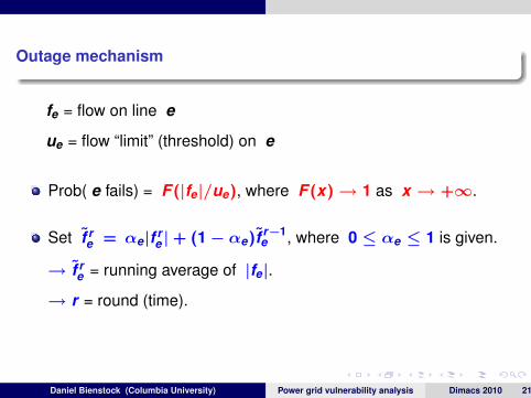
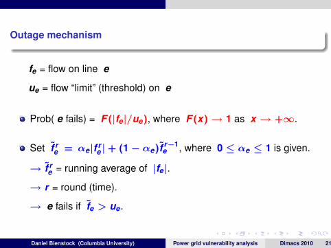
Outage mechanism
fe = flow on line e
ue = flow “limit” (threshold) on e
Prob( e fails) = F (|fe|/ue), where F (x) → 1 as x → +∞.
Set f re = αe|f r
e | + (1 − αe)f r−1e , where 0 ≤ αe ≤ 1 is given.
→ f re = running average of |fe|.
→ r = round (time).
→ e fails if fe > ue. or: e fails if fe ≥ ue
Daniel Bienstock (Columbia University) Power grid vulnerability analysis Dimacs 2010 21 / 45
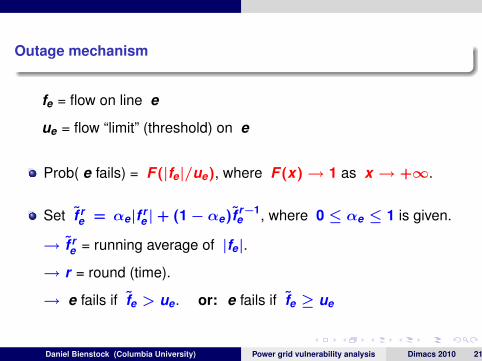
Outage mechanism
fe = flow on line e
ue = flow “limit” (threshold) on e
Prob( e fails) = F (|fe|/ue), where F (x) → 1 as x → +∞.
Set f re = αe|f r
e | + (1 − αe)f r−1e , where 0 ≤ αe ≤ 1 is given.
→ f re = running average of |fe|.
→ r = round (time).
→ e fails if fe > ue.
or: e fails if fe ≥ ue
Daniel Bienstock (Columbia University) Power grid vulnerability analysis Dimacs 2010 21 / 45
Outage mechanism
fe = flow on line e
ue = flow “limit” (threshold) on e
Prob( e fails) = F (|fe|/ue), where F (x) → 1 as x → +∞.
Set f re = αe|f r
e | + (1 − αe)f r−1e , where 0 ≤ αe ≤ 1 is given.
→ f re = running average of |fe|.
→ r = round (time).
→ e fails if fe > ue. or: e fails if fe ≥ ue
Daniel Bienstock (Columbia University) Power grid vulnerability analysis Dimacs 2010 21 / 45

Outage mechanism
fe = flow on line e
ue = flow “limit” (threshold) on e
Prob( e fails) = F (|fe|/ue), where F (x) → 1 as x → +∞.
Set f re = αe|f r
e | + (1 − αe)|f r−1e |, where 0 ≤ αe ≤ 1 is given.
→ f re = two-round average of |fe|.
→ r = round (time).
→ e fails if fe > ue,
(or, e fails if fe ≥ ue)
Daniel Bienstock (Columbia University) Power grid vulnerability analysis Dimacs 2010 22 / 45

Outage mechanism
fe = flow on line e
ue = flow “limit” (threshold) on e
Prob( e fails) = F (|fe|/ue), where F (x) → 1 as x → +∞.
Set f re = αe|f r
e | + (1 − αe)|f r−1e |, where 0 ≤ αe ≤ 1 is given.
→ f re = two-round average of |fe|.
→ r = round (time).
→ e fails if fe > ue, (or, e fails if fe ≥ ue)
Daniel Bienstock (Columbia University) Power grid vulnerability analysis Dimacs 2010 22 / 45
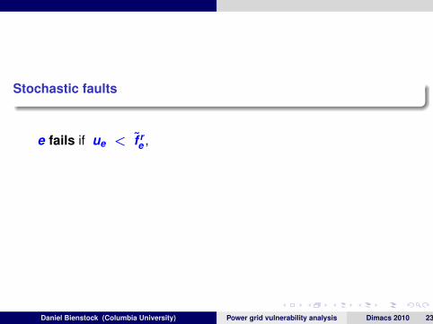
Stochastic faults
e fails if ue < f re ,
e does not fail if (1 − γ)ue > f re , (γ = tolerance)
if (1 − γ)ue ≤ f re ≤ ue then e fails with probability 1/2
Daniel Bienstock (Columbia University) Power grid vulnerability analysis Dimacs 2010 23 / 45

Stochastic faults
e fails if ue < f re ,
e does not fail if (1 − γ)ue > f re , (γ = tolerance)
if (1 − γ)ue ≤ f re ≤ ue then e fails with probability 1/2
Daniel Bienstock (Columbia University) Power grid vulnerability analysis Dimacs 2010 23 / 45

Stochastic faults
e fails if ue < f re ,
e does not fail if (1 − γ)ue > f re , (γ = tolerance)
if (1 − γ)ue ≤ f re ≤ ue then e fails with probability 1/2
Daniel Bienstock (Columbia University) Power grid vulnerability analysis Dimacs 2010 23 / 45
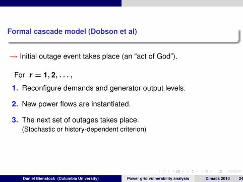
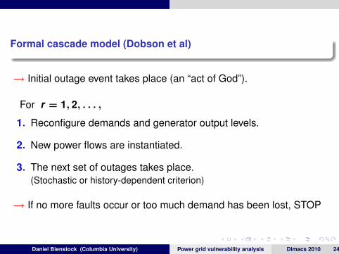
Formal cascade model (Dobson et al)
→ Initial outage event takes place (an “act of God”).
For r = 1, 2, . . . ,
1. Reconfigure demands and generator output levels.
2. New power flows are instantiated.
3. The next set of outages takes place.(Stochastic or history-dependent criterion)
→ If no more faults occur or too much demand has been lost, STOP
Daniel Bienstock (Columbia University) Power grid vulnerability analysis Dimacs 2010 24 / 45
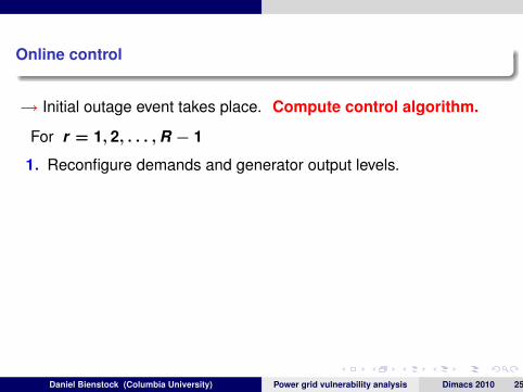
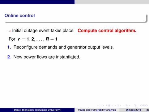
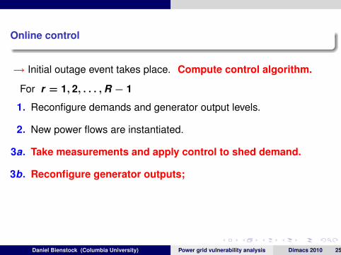
Online control
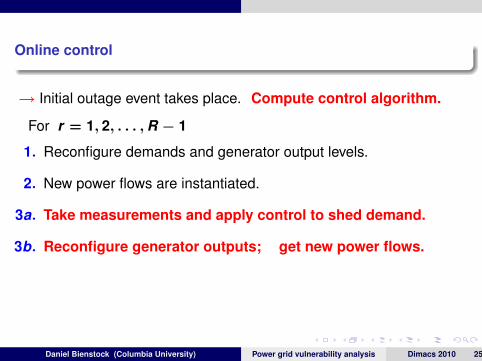
→ Initial outage event takes place.
Compute control algorithm.
For r = 1, 2, . . . , R − 1
1. Reconfigure demands and generator output levels.
2. New power flows are instantiated.
3a. Take measurements and apply control to shed demand.
3b. Reconfigure generator outputs; get new power flows.
4. The next set of outages takes place.
At round R, reduce demands so as to remove any line overloads.
Daniel Bienstock (Columbia University) Power grid vulnerability analysis Dimacs 2010 25 / 45
Online control
→ Initial outage event takes place. Compute control algorithm.
For r = 1, 2, . . . , R − 1
1. Reconfigure demands and generator output levels.
2. New power flows are instantiated.
3a. Take measurements and apply control to shed demand.
3b. Reconfigure generator outputs; get new power flows.
4. The next set of outages takes place.
At round R, reduce demands so as to remove any line overloads.
Daniel Bienstock (Columbia University) Power grid vulnerability analysis Dimacs 2010 25 / 45
Online control
→ Initial outage event takes place. Compute control algorithm.
For r = 1, 2, . . . , R − 1
1. Reconfigure demands and generator output levels.
2. New power flows are instantiated.
3a. Take measurements and apply control to shed demand.
3b. Reconfigure generator outputs;
get new power flows.
4. The next set of outages takes place.
At round R, reduce demands so as to remove any line overloads.
Daniel Bienstock (Columbia University) Power grid vulnerability analysis Dimacs 2010 25 / 45
Online control
→ Initial outage event takes place. Compute control algorithm.
For r = 1, 2, . . . , R − 1
1. Reconfigure demands and generator output levels.
2. New power flows are instantiated.
3a. Take measurements and apply control to shed demand.
3b. Reconfigure generator outputs; get new power flows.
4. The next set of outages takes place.
At round R, reduce demands so as to remove any line overloads.
Daniel Bienstock (Columbia University) Power grid vulnerability analysis Dimacs 2010 25 / 45

Deterministic, no history model
“Optimal” control via integer programming formulation
?
f rj = flow on arc j at round r
y rj = 1, if arc j fails in round r , 0 otherwise
d rj = demand at node i in round r
and many other variables
Daniel Bienstock (Columbia University) Power grid vulnerability analysis Dimacs 2010 26 / 45

Deterministic, no history model
“Optimal” control via integer programming formulation ?
f rj = flow on arc j at round r
y rj = 1, if arc j fails in round r , 0 otherwise
d rj = demand at node i in round r
and many other variables
Daniel Bienstock (Columbia University) Power grid vulnerability analysis Dimacs 2010 26 / 45
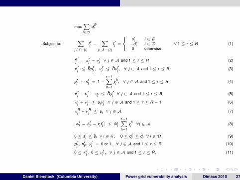
maxXi∈D
dRi
Subject to:X
j∈δ+(i)
f rj −
Xj∈δ−(i)
f rj =
8<: sri i ∈ G
−d ri i ∈ D
0 otherwise∀ 1 ≤ r ≤ R (1)
f rj = π
rj − ν
rj ∀ j ∈ A and 1 ≤ r ≤ R (2)
πrj ≤ Dpr
j , νrj ≤ Dnr
j , ∀ j ∈ A and 1 ≤ r ≤ R (3)
prj + nr
j = 1 −r−1Xh=1
yhj , ∀ j ∈ A and 1 ≤ r ≤ R (4)
πrj + ν
rj − uj ≤ Dy r
j ∀ j ∈ A and 1 ≤ r ≤ R (5)
πrj + ν
rj ≥ uj y
rj ∀ j ∈ A and 1 ≤ r ≤ R − 1 (6)
πRj + ν
Rj ≤ uj ∀ j ∈ A (7)
|φri − φ
rj − xj f
rj | ≤ Mj
r−1Xh=1
yhj ∀j ∈ A (8)
0 ≤ sri ≤ si ∀ i ∈ G, 0 ≤ d r
i ≤ di ∀ i ∈ D, (9)
prj , nr
ij , y rj = 0 or 1, ∀ j ∈ A and 1 ≤ r ≤ R (10)
0 ≤ πrj , 0 ≤ ν
rj , ∀ j ∈ A and 1 ≤ r ≤ R. (11)
Daniel Bienstock (Columbia University) Power grid vulnerability analysis Dimacs 2010 27 / 45

What’s bad about the formulation
probably can’t solve it for medium to large networks
stochastic variant probably needed, harder
optimal solutions = complex policies
Daniel Bienstock (Columbia University) Power grid vulnerability analysis Dimacs 2010 28 / 45

What’s bad about the formulation
probably can’t solve it for medium to large networks
stochastic variant probably needed, harder
optimal solutions = complex policies
Daniel Bienstock (Columbia University) Power grid vulnerability analysis Dimacs 2010 28 / 45
Adaptive affine controls
For each demand v , and round r , control crv , br
v , srv to be
computed
→ Parameterized by integer r > 0.
At round r ,
Let κ = maximum overload of any line within radius r of v
If κ > crv , demand at v reduced (scaled) by a factor
max{
1, srv (cr
v − κ) + brv}
.
The goal: pick control to maximize demand being served at the end ofround R.
Daniel Bienstock (Columbia University) Power grid vulnerability analysis Dimacs 2010 29 / 45
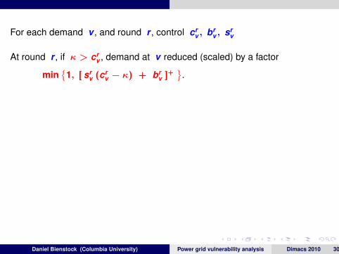
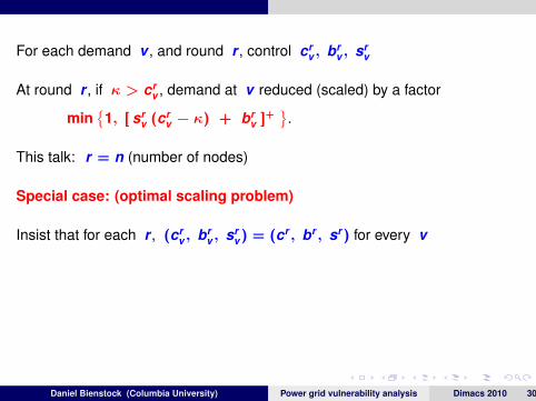
For each demand v , and round r , control crv , br
v , srv
At round r , if κ > crv , demand at v reduced (scaled) by a factor
min{
1, [ srv (cr
v − κ) + brv ]+
}.
This talk: r = n (number of nodes)
Special case: (optimal scaling problem)
Insist that for each r , (crv , br
v , srv) = (cr , br , sr) for every v
Then, equivalent problem:
In round r , let αr(K ) ≤ 1 be chosen for each component of thenetwork in round r
If node v ∈ component K , then its demand is scaled by αr(K )
Daniel Bienstock (Columbia University) Power grid vulnerability analysis Dimacs 2010 30 / 45

Notation:
β = supply/demand vector at time 0
f = corresponding power flows at time 0
ΘR(t, β) : R+ → R+ = total demand, at the end of round R, usingoptimal control, if the supply/demand vector is t β
Note: supply/demand = tβ means flow = t f
Theorem:
ΘR(t, β) is nondecreasing piecewise-linear with at mostmR/R! + O(mR−1) breakpoints. m = no. of arcs
In round 1, the optimal scale is equal to uj/(t fj) for some arc j .So arc j will become critical
And recursively ...
Robust/stochastic version?
Daniel Bienstock (Columbia University) Power grid vulnerability analysis Dimacs 2010 31 / 45

Notation:
β = supply/demand vector at time 0
f = corresponding power flows at time 0
ΘR(t, β) : R+ → R+ = total demand, at the end of round R, usingoptimal control, if the supply/demand vector is t β
Note: supply/demand = tβ means flow = t f
Theorem:
ΘR(t, β) is nondecreasing piecewise-linear with at mostmR/R! + O(mR−1) breakpoints. m = no. of arcs
In round 1, the optimal scale is equal to uj/(t fj) for some arc j .
So arc j will become critical
And recursively ...
Robust/stochastic version?
Daniel Bienstock (Columbia University) Power grid vulnerability analysis Dimacs 2010 31 / 45

Notation:
β = supply/demand vector at time 0
f = corresponding power flows at time 0
ΘR(t, β) : R+ → R+ = total demand, at the end of round R, usingoptimal control, if the supply/demand vector is t β
Note: supply/demand = tβ means flow = t f
Theorem:
ΘR(t, β) is nondecreasing piecewise-linear with at mostmR/R! + O(mR−1) breakpoints. m = no. of arcs
In round 1, the optimal scale is equal to uj/(t fj) for some arc j .So arc j will become critical
And recursively ...
Robust/stochastic version?
Daniel Bienstock (Columbia University) Power grid vulnerability analysis Dimacs 2010 31 / 45

Notation:
β = supply/demand vector at time 0
f = corresponding power flows at time 0
ΘR(t, β) : R+ → R+ = total demand, at the end of round R, usingoptimal control, if the supply/demand vector is t β
Note: supply/demand = tβ means flow = t f
Theorem:
ΘR(t, β) is nondecreasing piecewise-linear with at mostmR/R! + O(mR−1) breakpoints. m = no. of arcs
In round 1, the optimal scale is equal to uj/(t fj) for some arc j .So arc j will become critical
And recursively ...
Robust/stochastic version?
Daniel Bienstock (Columbia University) Power grid vulnerability analysis Dimacs 2010 31 / 45

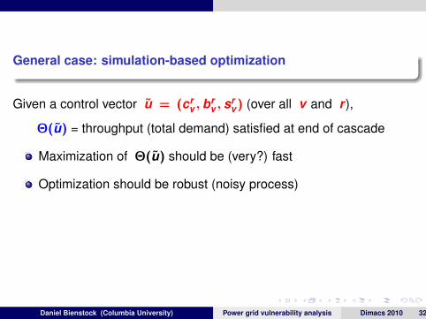
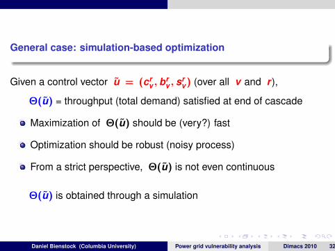
General case: simulation-based optimization
Given a control vector u = (crv , br
v , srv) (over all v and r ),
Θ(u) = throughput (total demand) satisfied at end of cascade
Maximization of Θ(u) should be (very?) fast
Optimization should be robust (noisy process)
From a strict perspective, Θ(u) is not even continuous
Θ(u) is obtained through a simulation
Daniel Bienstock (Columbia University) Power grid vulnerability analysis Dimacs 2010 32 / 45

Derivative-free optimization
Conn, Scheinberg, Vicente, others
Rough description:
Sample a number of control vectors u
Use the sample points to construct a convex approximation to Θ
Optimize this approximation; this yields a new sample point
Scalability to large dimensionality?
Daniel Bienstock (Columbia University) Power grid vulnerability analysis Dimacs 2010 33 / 45

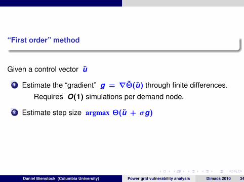
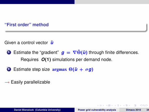
“First order” method
Given a control vector u
1 Estimate the “gradient” g = ∇Θ(u) through finite differences.
Requires O(1) simulations per demand node.
2 Estimate step size argmax Θ(u + σg)
→ Easily parallelizable
Daniel Bienstock (Columbia University) Power grid vulnerability analysis Dimacs 2010 34 / 45
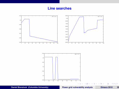
Line searches
0.85
0.86
0.87
0.88
0.89
0.9
0.91
0 10 20 30 40 50 60 70 80 90 100
ls3.1
0.9155
0.916
0.9165
0.917
0.9175
0.918
0.9185
0.919
0.9195
0.92
0.9205
0 10 20 30 40 50 60 70 80 90 100
ls3.2
0.25
0.3
0.35
0.4
0.45
0.5
0.55
0 10 20 30 40 50 60 70 80
ls4.2
Daniel Bienstock (Columbia University) Power grid vulnerability analysis Dimacs 2010 35 / 45

Current parallel implementation: boss-nerd
Boss carries out search algorithm
Nerds simulate cascades with given control
Communication using Unix sockets
Daniel Bienstock (Columbia University) Power grid vulnerability analysis Dimacs 2010 36 / 45

Scaling
Example: 10000 nodes, 19309 lines
5 gradient steps
8-core i7 CPUs (3 machines total)
cores wall-clock sec2 943794 475928 2813616 1461824 9918
Daniel Bienstock (Columbia University) Power grid vulnerability analysis Dimacs 2010 37 / 45

Initial experiments with Eastern Interconnect
15023 nodes, 23769 lines.
2122 generator nodes, 6261 demand nodes
“Equivalent” DC flow version
Methodology for experiments1 Generate an interdiction of the grid (“initial event”)2 Compute control and simulate3 At least three rounds of cascade after initial event
Daniel Bienstock (Columbia University) Power grid vulnerability analysis Dimacs 2010 38 / 45

Initial experiments with Eastern Interconnect
15023 nodes, 23769 lines.
2122 generator nodes, 6261 demand nodes
“Equivalent” DC flow version
Methodology for experiments1 Generate an interdiction of the grid (“initial event”)2 Compute control and simulate
3 At least three rounds of cascade after initial event
Daniel Bienstock (Columbia University) Power grid vulnerability analysis Dimacs 2010 38 / 45

Initial experiments with Eastern Interconnect
15023 nodes, 23769 lines.
2122 generator nodes, 6261 demand nodes
“Equivalent” DC flow version
Methodology for experiments1 Generate an interdiction of the grid (“initial event”)2 Compute control and simulate3 At least three rounds of cascade after initial event
Daniel Bienstock (Columbia University) Power grid vulnerability analysis Dimacs 2010 38 / 45
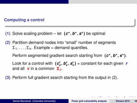
Computing a control
(1) Solve scaling problem – let (c∗, b∗, s∗) be optimal
(2) Partition demand nodes into “small” number of segmentsΣ1, . . . ,Σk . Example = demand quantiles.
Perform segmented gradient search starting from (c∗, b∗, s∗).
Look for a control with (crv , br
v , srv) = constant for each given r
and all v in a common Σi .
(3) Perform full gradient search starting from the output in (2).
Daniel Bienstock (Columbia University) Power grid vulnerability analysis Dimacs 2010 39 / 45
Computing a control
(1) Solve scaling problem – let (c∗, b∗, s∗) be optimal
(2) Partition demand nodes into “small” number of segmentsΣ1, . . . ,Σk .
Example = demand quantiles.
Perform segmented gradient search starting from (c∗, b∗, s∗).
Look for a control with (crv , br
v , srv) = constant for each given r
and all v in a common Σi .
(3) Perform full gradient search starting from the output in (2).
Daniel Bienstock (Columbia University) Power grid vulnerability analysis Dimacs 2010 39 / 45
Computing a control
(1) Solve scaling problem – let (c∗, b∗, s∗) be optimal
(2) Partition demand nodes into “small” number of segmentsΣ1, . . . ,Σk . Example = demand quantiles.
Perform segmented gradient search starting from (c∗, b∗, s∗).
Look for a control with (crv , br
v , srv) = constant for each given r
and all v in a common Σi .
(3) Perform full gradient search starting from the output in (2).
Daniel Bienstock (Columbia University) Power grid vulnerability analysis Dimacs 2010 39 / 45

Experiments
K random lines taken out
highly loaded lines more likely to be taken out; connectivity preserved
K yield, (%) yield, wallclockno control control (sec)
1 90.04 95.03 1342 12.54 50.13 875 32.94 81.05 10710 2.02 36.97 9720 1.64 27.84 15950 0.83 16.96 209
Daniel Bienstock (Columbia University) Power grid vulnerability analysis Dimacs 2010 40 / 45

Conjectures
It is best to stop the cascade in the first round
It is best to apply control in the first round only, and ride out thecascade
(Answer: both wrong)
Daniel Bienstock (Columbia University) Power grid vulnerability analysis Dimacs 2010 41 / 45

Conjectures
It is best to stop the cascade in the first round
It is best to apply control in the first round only, and ride out thecascade
(Answer: both wrong)
Daniel Bienstock (Columbia University) Power grid vulnerability analysis Dimacs 2010 41 / 45

Details: cascade with 50 (highly loaded) random lines taken out
No control ⇒ yield = 0%
Optimal round 1 only constant control ⇒ yield = 38%
Optimal scaling control ⇒ yield = 45%
Plus segmented gradient seach ⇒ yield = 50%
Daniel Bienstock (Columbia University) Power grid vulnerability analysis Dimacs 2010 42 / 45

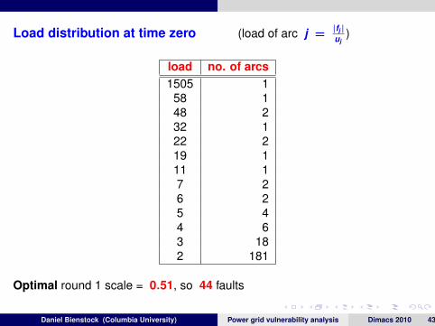
Load distribution at time zero (load of arc j =|fj |uj
)
load no. of arcs1505 1
58 148 232 122 219 111 17 26 25 44 63 182 181
Optimal round 1 scale = 0.51, so 44 faults
Daniel Bienstock (Columbia University) Power grid vulnerability analysis Dimacs 2010 43 / 45

Load distribution at time zero (load of arc j =|fj |uj
)
load no. of arcs1505 1
58 148 232 122 219 111 17 26 25 44 63 182 181
Optimal round 1 scale = 0.51,
so 44 faults
Daniel Bienstock (Columbia University) Power grid vulnerability analysis Dimacs 2010 43 / 45
Load distribution at time zero (load of arc j =|fj |uj
)
load no. of arcs1505 1
58 148 232 122 219 111 17 26 25 44 63 182 181
Optimal round 1 scale = 0.51, so 44 faults
Daniel Bienstock (Columbia University) Power grid vulnerability analysis Dimacs 2010 43 / 45
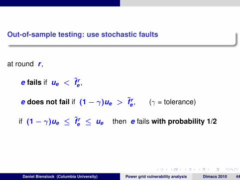
Out-of-sample testing: use stochastic faults
at round r ,
e fails if ue < f re ,
e does not fail if (1 − γ)ue > f re , (γ = tolerance)
if (1 − γ)ue ≤ f re ≤ ue then e fails with probability 1/2
What is the impact of γ?
Daniel Bienstock (Columbia University) Power grid vulnerability analysis Dimacs 2010 44 / 45
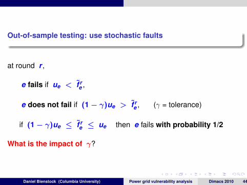
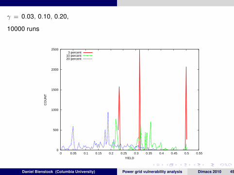
γ = 0.03, 0.10, 0.20,
10000 runs
0
500
1000
1500
2000
2500
0 0.05 0.1 0.15 0.2 0.25 0.3 0.35 0.4 0.45 0.5 0.55
CO
UN
T
YIELD
3 percent10 percent20 percent
Daniel Bienstock (Columbia University) Power grid vulnerability analysis Dimacs 2010 45 / 45


![Power Grid Vulnerability to Geographically …...to physical attacks, such as an Electromagnetic Pulse (EMP) attack [17], [34]. Thus, we focus on the vulnerability of the power grid](https://img.pdfslide.net/doc/110x75/5f598366158abd33eb72043e/power-grid-vulnerability-to-geographically-to-physical-attacks-such-as-an-electromagnetic.jpg)