Embed Size (px)
Citation preview

Power Iteration ClusteringFrank Lin and William W. Cohen
School of Computer Science, Carnegie Mellon University
ICML 20102010-06-23, Haifa, Israel

Overview
• Preview• Motivation• Power Iteration Clustering– Power Iteration– Stopping
• Results• Related Work

Overview
• Preview• Motivation• Power Iteration Clustering– Power Iteration– Stopping
• Results• Related Work

Preview
• Spectral clustering methods are nice

Preview
• Spectral clustering methods are nice• But they are rather expensive (slow)

Preview
• Spectral clustering methods are nice• But they are rather expensive (slow)
Power iteration clustering can provide a similar solution at a
very low cost (fast)

Preview: Runtime
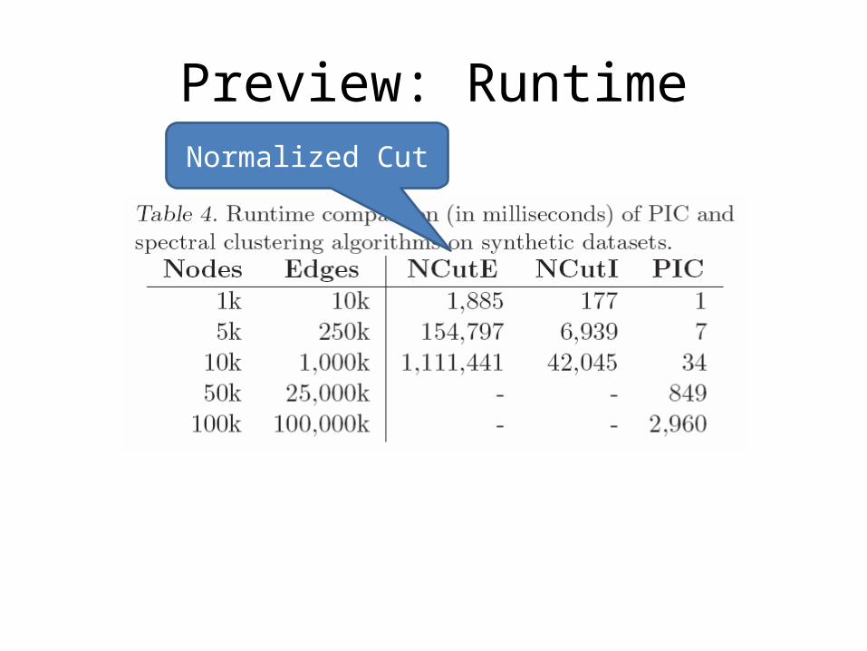
Preview: RuntimeNormalized Cut
Preview: RuntimeNormalized Cut Normalized Cut, faster
implementation

Preview: RuntimeNormalized Cut Normalized Cut, faster
implementation
Pretty fast

Preview: RuntimeNormalized Cut Normalized Cut, faster
implementation
Ran out of memory (24GB)

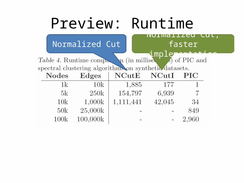
Preview: Accuracy
Preview: Accuracy
Upper triangle: PIC does
better

Preview: Accuracy
Upper triangle: PIC does
better
Lower triangle: NCut or
NJW does better

Overview
• Preview• Motivation• Power Iteration Clustering– Power Iteration– Stopping
• Results• Related Work
k-means
• A well-known clustering method

k-means
• A well-known clustering method• 3-cluster examples:

k-means
• A well-known clustering method• 3-cluster examples:
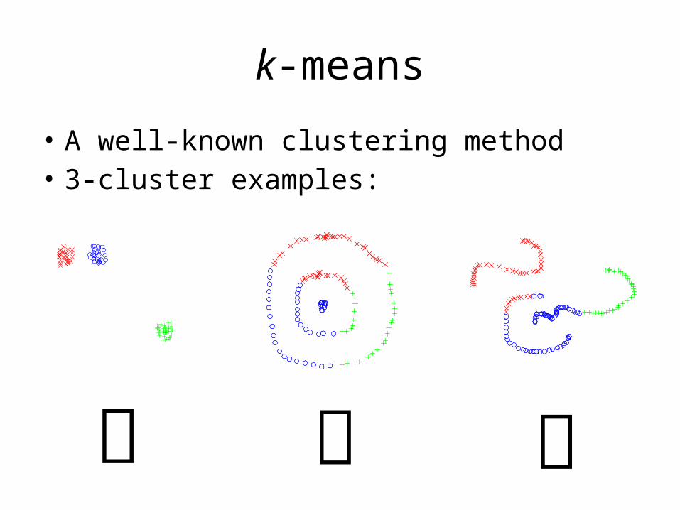
k-means
• A well-known clustering method• 3-cluster examples:

Spectral Clustering
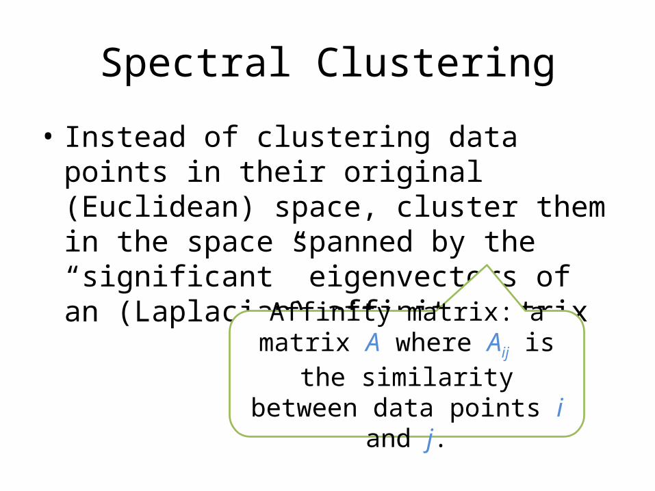
• Instead of clustering data points in their original (Euclidean) space, cluster them in the space spanned by the “significant” eigenvectors of an (Laplacian) affinity matrix
Spectral Clustering
• Instead of clustering data points in their original (Euclidean) space, cluster them in the space spanned by the “significant” eigenvectors of an (Laplacian) affinity matrix
Affinity matrix: a matrix A where Aij is the similarity
between data points i and j.

Spectral Clustering
• Network = Graph = Matrix
AB
C
FD
E
GI
HJ
A B C D E F G H I J
A 1 1 1
B 1 1
C 1
D 1 1
E 1
F 1 1 1
G 1
H 1 1
I 1 1 1
J 1 1

Spectral Clustering
• Results with Normalized Cuts:

Spectral Clusteringdataset and normalized cut results
2nd eigenvector
3rd eigenvector

Spectral Clusteringdataset and normalized cut results
2nd eigenvector
3rd eigenvector
valu
e
index
1 2 3cluster

Spectral Clusteringdataset and normalized cut results
2nd smallest eigenvector
3rd smallest eigenvector
valu
e
index
1 2 3cluster
clus
terin
g s
pace
Spectral Clustering
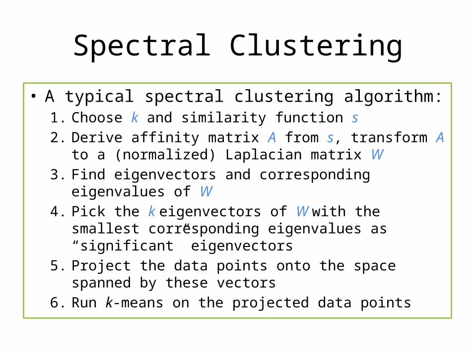
• A typical spectral clustering algorithm:1. Choose k and similarity function s2. Derive affinity matrix A from s, transform A to a
(normalized) Laplacian matrix W3. Find eigenvectors and corresponding eigenvalues of W4. Pick the k eigenvectors of W with the smallest
corresponding eigenvalues as “significant” eigenvectors5. Project the data points onto the space spanned by these
vectors6. Run k-means on the projected data points

Spectral Clustering
• Normalized Cut algorithm (Shi & Malik 2000):1. Choose k and similarity function s2. Derive A from s, let W=I-D-1A, where I is the identity
matrix and D is a diagonal square matrix Dii=Σj Aij
3. Find eigenvectors and corresponding eigenvalues of W4. Pick the k eigenvectors of W with the 2nd to kth smallest
corresponding eigenvalues as “significant” eigenvectors5. Project the data points onto the space spanned by these
vectors6. Run k-means on the projected data points
D
Finding eigenvectors and eigenvalues of a matrix is very slow
in general: O(n3)

Hmm…
• Can we find a low-dimensional embedding for clustering, as spectral clustering, but without calculating these eigenvectors?

Overview
• Preview• Motivation• Power Iteration Clustering– Power Iteration– Stopping
• Results• Related Work
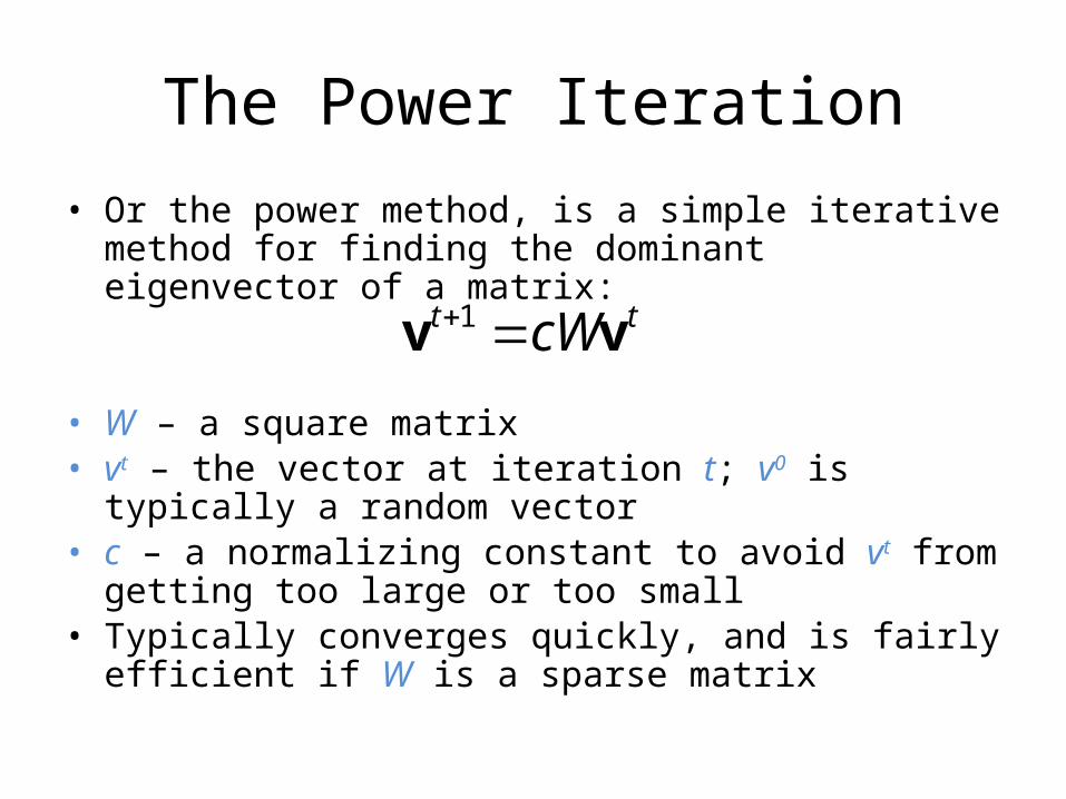
The Power Iteration• Or the power method, is a simple iterative method for finding
the dominant eigenvector of a matrix:
• W – a square matrix• vt – the vector at iteration t; v0 is typically a random vector• c – a normalizing constant to avoid vt from getting too large or
too small• Typically converges quickly, and is fairly efficient if W is a
sparse matrix
tt cWvv 1

The Power Iteration• Or the power method, is a simple iterative method for finding
the dominant eigenvector of a matrix:
• What if we let W=D-1A (similar to Normalized Cut)?
tt cWvv 1

The Power Iteration• Or the power method, is a simple iterative method for finding
the dominant eigenvector of a matrix:
• What if we let W=D-1A (similar to Normalized Cut)?• The short answer is that it converges to a constant vector,
because the dominant eigenvector of a row-normalized matrix is always a constant vector
• Not very interesting. However…
tt cWvv 1

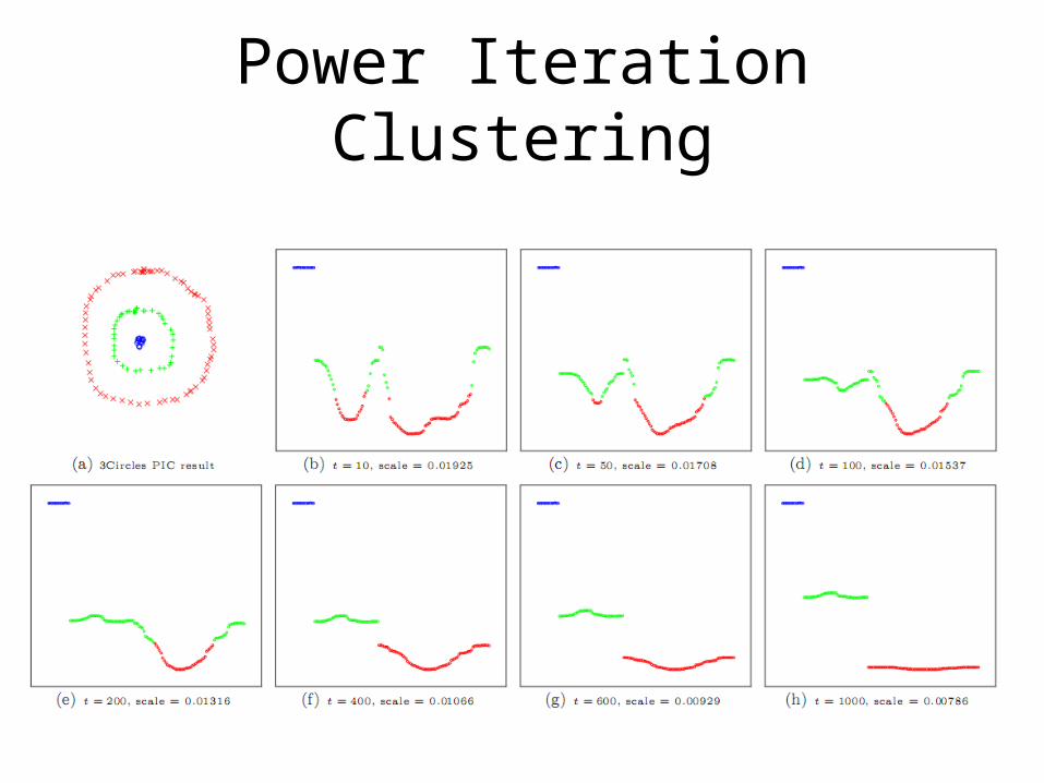
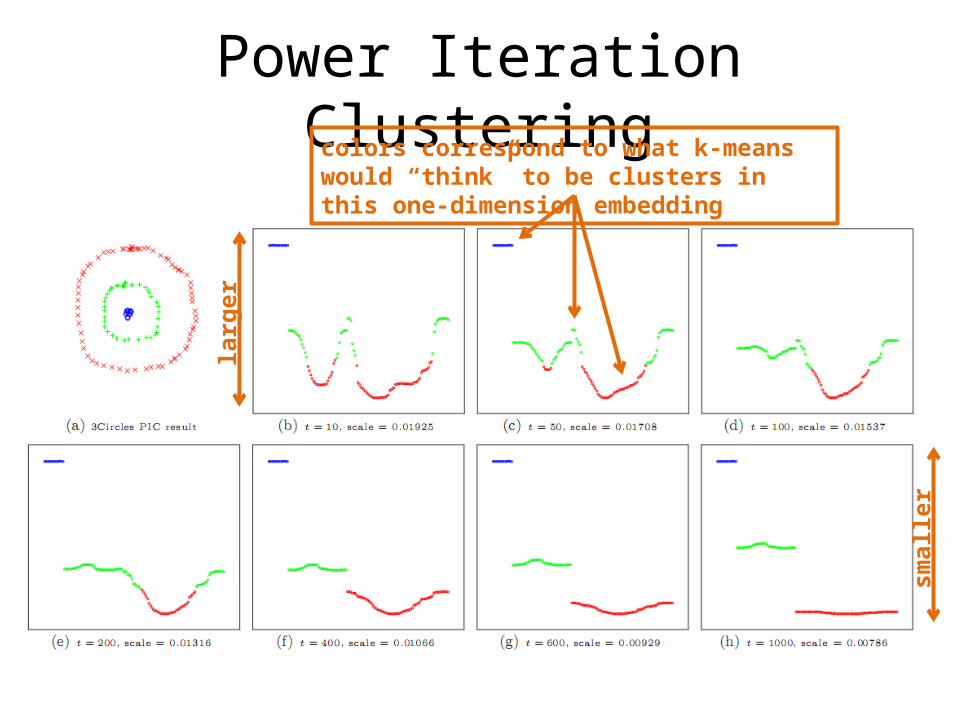
Power Iteration Clustering
• It turns out that, if there is some underlying cluster in the data, PI will quickly converge locally within clusters then slowly converge globally to a constant vector.
• The locally converged vector, which is a linear combination of the top eigenvectors, will be nearly piece-wise constant with each piece corresponding to a cluster
Power Iteration Clustering
Power Iteration Clustering
smal
ler
larg
er
colors correspond to what k-means would “think” to be clusters in this one-dimension embedding

Power Iteration Clustering• Recall the power iteration update:
ntnn
tt
nt
ntt
t
t
tt
ccc
WcWcWc
W
W
W
eee
eee
v
v
vv
...
...
...
222111
2211
0
22
1

Power Iteration Clustering• Recall the power iteration update:
ntnn
tt
nt
ntt
t
t
tt
ccc
WcWcWc
W
W
W
eee
eee
v
v
vv
...
...
...
222111
2211
0
22
1
λi - the ith largest eigenvalue of W
ci - the ith coefficient of v when projected
onto the space spanned by the
eigenvectors of W
ei – the eigenvector corresponding to λi

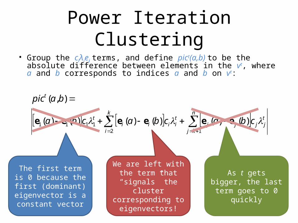
Power Iteration Clustering• Group the ciλiei terms, and define pict(a,b) to be the absolute
difference between elements in the vt, where a and b corresponds to indices a and b on vt:
n
kj
tjjjj
k
i
tiiii
t
t
cbacbacba
bapic
121111 )()()()()()(
),(
eeeeee

Power Iteration Clustering• Group the ciλiei terms, and define pict(a,b) to be the absolute
difference between elements in the vt, where a and b corresponds to indices a and b on vt:
n
kj
tjjjj
k
i
tiiii
t
t
cbacbacba
bapic
121111 )()()()()()(
),(
eeeeee
The first term is 0 because the first
(dominant) eigenvector is a constant vector
As t gets bigger, the last term goes to 0 quickly
We are left with the term that “signals” the cluster corresponding
to eigenvectors!

Power Iteration Clustering
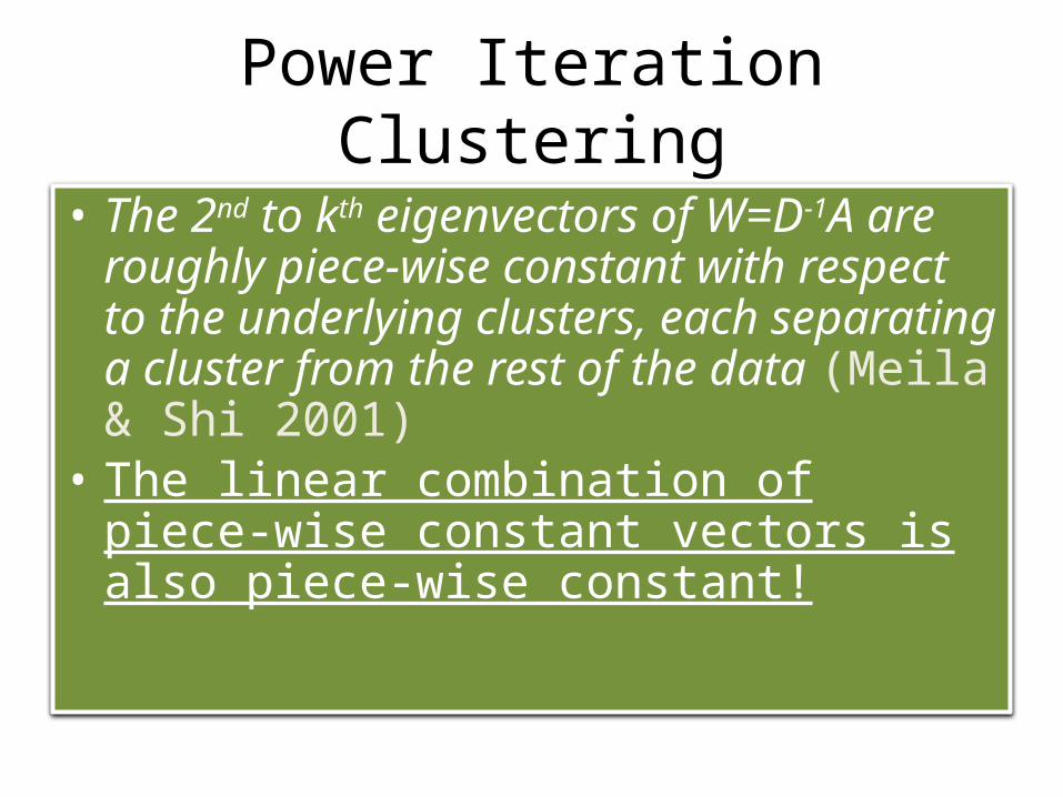
• The 2nd to kth eigenvectors of W=D-1A are roughly piece-wise constant with respect to the underlying clusters, each separating a cluster from the rest of the data (Meila & Shi 2001)
Power Iteration Clustering
• The 2nd to kth eigenvectors of W=D-1A are roughly piece-wise constant with respect to the underlying clusters, each separating a cluster from the rest of the data (Meila & Shi 2001)
• The linear combination of piece-wise constant vectors is also piece-wise constant!

Spectral Clusteringdataset and normalized cut results
2nd smallest eigenvector
3rd smallest eigenvector
valu
e
index
1 2 3cluster
clus
terin
g s
pace

Spectral Clusteringdataset and normalized cut results
2nd smallest eigenvector
3rd smallest eigenvector
valu
e
index
clus
terin
g s
pace

Spectral Clustering
2nd smallest eigenvector
3rd smallest eigenvector


a·
b·
+

a·
b·
+
=

a·
b·
+
=

Power Iteration Clustering
Power Iteration Clustering
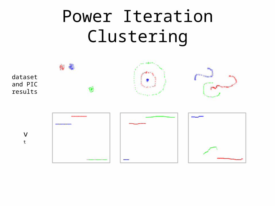
dataset and PIC results
vt

Power Iteration Clustering
dataset and PIC results
vt
The Take-Away
To do clustering, we may not need all the information in a spectral embedding (e.g., distance between clusters in a k-dimension eigenspace); we just need the clusters to be separated in some space.
Power Iteration Clustering
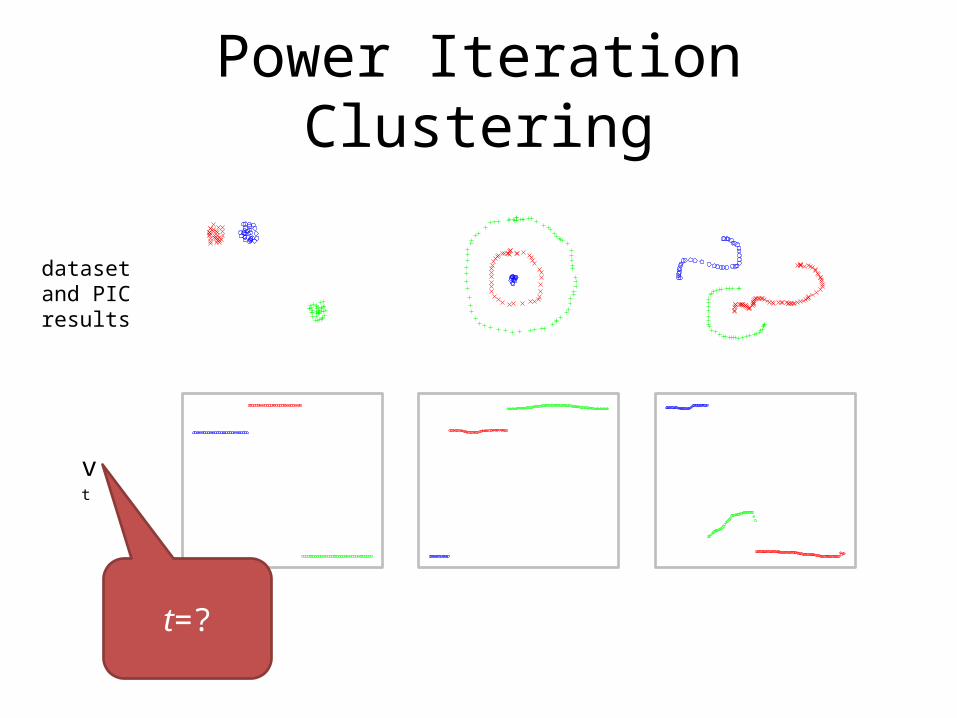
dataset and PIC results
vt
t=?

Power Iteration Clustering
dataset and PIC results
vt
t=? Want to iterate enough to show clusters, but not too much so as to converge to a constant
vector

Overview
• Preview• Motivation• Power Iteration Clustering– Power Iteration– Stopping
• Results• Related Work

When to Stop
ntnnk
tkkk
tkk
tt cccc eeeev ...... 111111
Recall:

When to Stop
ntnnk
tkkk
tkk
tt cccc eeeev ...... 111111
Recall:
n
t
nnk
t
kkk
t
kkt
t
c
c
c
c
c
c
ceeee
v
111
1
1
1
1
111
11
......
Then:

When to Stop
ntnnk
tkkk
tkk
tt cccc eeeev ...... 111111
Recall:
n
t
nnk
t
kkk
t
kkt
t
c
c
c
c
c
c
ceeee
v
111
1
1
1
1
111
11
......
Then:
Because they are raised to the power t, the eigenvalue ratios
determines how fast v converges to e1

When to Stop
ntnnk
tkkk
tkk
tt cccc eeeev ...... 111111
Recall:
n
t
nnk
t
kkk
t
kkt
t
c
c
c
c
c
c
ceeee
v
111
1
1
1
1
111
11
......
Then:
Because they are raised to the power t, the eigenvalue ratios
determines how fast v converges to e1
At the beginning, v changes fast (“accelerating”) to converge locally due to “noise terms”
(k+1…n) with small λ
When “noise terms” have gone to zero, v changes slowly (“constant speed”) because only larger λ terms (2…k) are left, where the
eigenvalue ratios are close to 1

When to Stop
• So we can stop when the “acceleration” is nearly zero.

When to Stop
ntnnk
tkkk
tkk
tt cccc eeeev ...... 111111
Recall:
n
t
nnk
t
kkk
t
t
t
c
c
c
c
c
c
ceeee
v
111
1
1
1
1
1
2
1
21
11
......
Then:
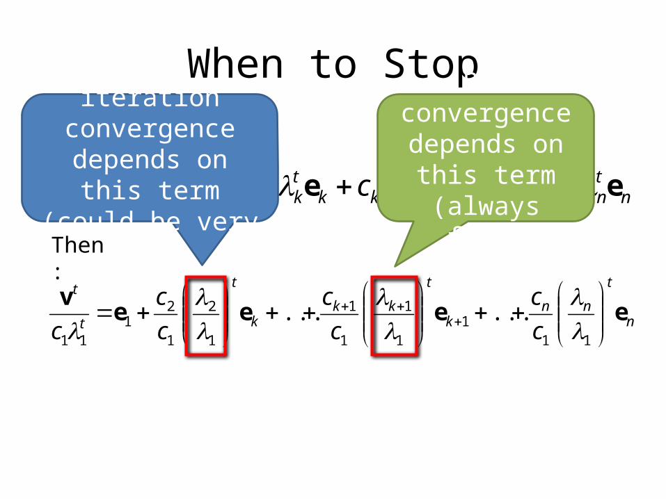
Power iteration convergence depends
on this term (could be very slow)
When to Stop
ntnnk
tkkk
tkk
tt cccc eeeev ...... 111111
Recall:
n
t
nnk
t
kkk
t
t
t
c
c
c
c
c
c
ceeee
v
111
1
1
1
1
1
2
1
21
11
......
Then:
Power iteration convergence depends
on this term (could be very slow)
PIC convergence depends on this
term (always fast)

Algorithm
• A basic power iteration clustering algorithm:
Input: A row-normalized affinity matrix W and the number of clusters kOutput: Clusters C1, C2, …, Ck
1. Pick an initial vector v0
2. Repeat• Set vt+1 ← Wvt
• Set δt+1 ← |vt+1 – vt|• Increment t• Stop when |δt – δt-1| ≈ 0
3. Use k-means to cluster points on vt and return clusters C1, C2, …, Ck

Overview
• Preview• Motivation• Power Iteration Clustering– Power Iteration– Stopping
• Results• Related Work

Results on Real Data• “Network” problems - natural graph structure:
– PolBooks 105 political books, 3 classes, linked by co-purchaser– UMBCBlog 404 political blogs, 2 classes, blog post links– AGBlog 1222 political blogs, 2 classes, blogroll links
• “Manifold” problems - cosine distance between instances:– Iris 150 flowers, 3 classes– PenDigits01 200 handwritten digits, 2 classes (“0” and “1”)– PenDigits17 200 handwritten digits, 2 classes (“1” and “7”)– 20ngA 200 docs, misc.forsale vs. soc.religion.christian– 20ngB 400 docs, misc.forsale vs. soc.religion.christian– 20ngC 20ngB + 200 docs from talk.politics.guns– 20ngD 20ngC + 200 docs from rec.sport.baseball

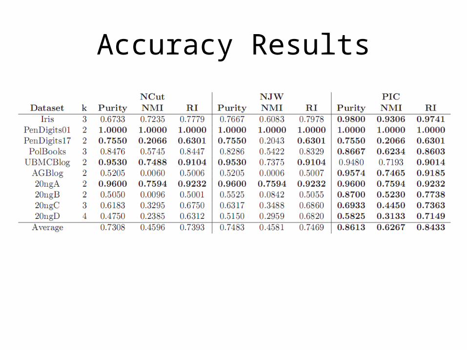
Accuracy Results
Upper triangle: PIC does
better
Lower triangle: NCut or
NJW does better

Accuracy Results

Accuracy Results

Runtime Speed Results
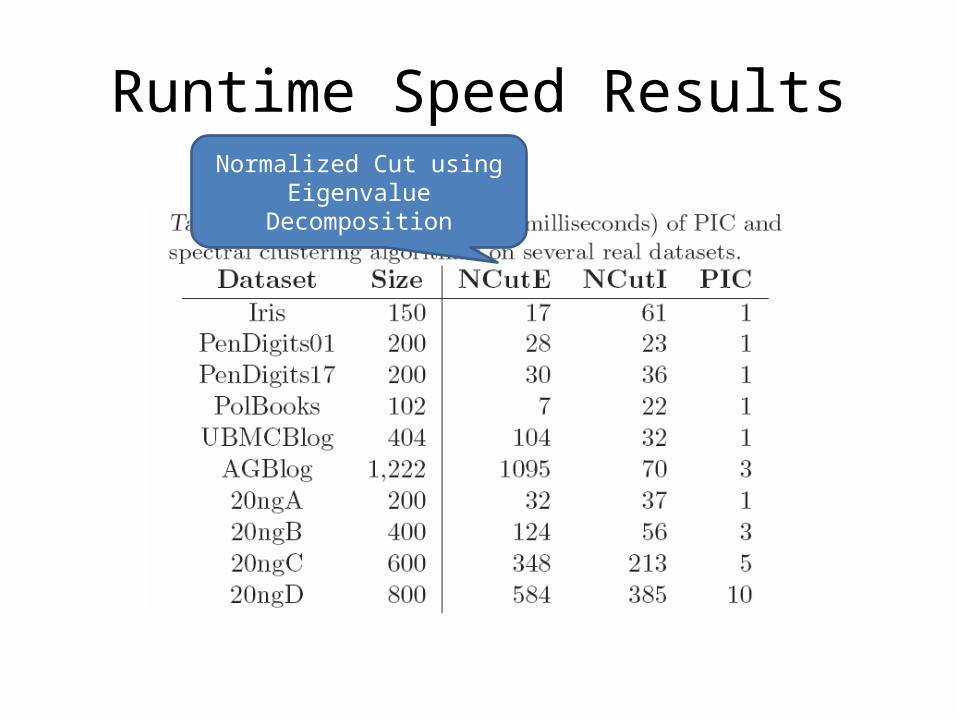
Runtime Speed ResultsNormalized Cut using
Eigenvalue Decomposition
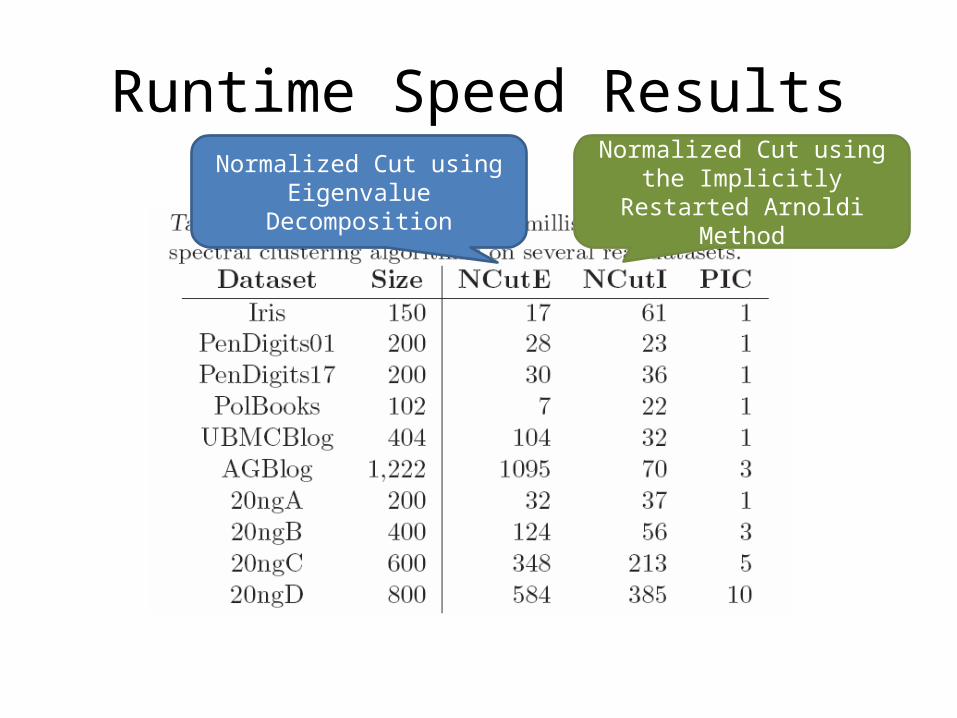
Runtime Speed ResultsNormalized Cut using
Eigenvalue Decomposition
Normalized Cut using the Implicitly Restarted Arnoldi
Method

Runtime Speed ResultsSome of
these ran in less than a millisecond

Runtime Speed Results

Runtime Speed ResultsModified version of Erdos-Renyi
with two similar-sized cluster per dataset

Runtime Speed Results
Ran out of memory (24GB)

Overview
• Preview• Motivation• Power Iteration Clustering– Power Iteration– Stopping
• Results• Related Work

Related Clustering Work• Spectral Clustering
– (Roxborough & Sen 1997, Shi & Malik 2000, Meila & Shi 2001, Ng et al. 2002)• Kernel k-Means (Dhillon et al. 2007)• Modularity Clustering (Newman 2006)• Matrix Powering
– Markovian relaxation & the information bottleneck method (Tishby & Slonim 2000)
– matrix powering (Zhou & Woodruff 2004)– diffusion maps (Lafon & Lee 2006)– Gaussian blurring mean-shift (Carreira-Perpinan 2006)
• Mean-Shift Clustering– mean-shift (Fukunaga & Hostetler 1975, Cheng 1995, Comaniciu & Meer 2002)– Gaussian blurring mean-shift (Carreira-Perpinan 2006)

Some “Powering” Methods at a Glance
Method W Iterate Stopping Final
Tishby & Slonim 2000 W=D-1A Wt+1=Wt
rate of information
loss
information bottleneck
method
Zhou & Woodruff
2004W=A Wt+1=Wt a small t a threshold ε
Carreira-Perpinan
2006W=D-1A Xt+1=WX entropy a threshold ε
PIC W=D-1A vt+1=Wvt acceleration k-means
How far can we go with a one- or low-dimensional
embedding?

Conclusion
• Fast• Space-efficient• Simple• Simple parallel/distributed implementation

Conclusion
• Fast• Space-efficient• Simple• Simple parallel/distributed implementation
• Plug: extensions for manifold problems with dense similarity matrices, without node/edge sampling (ECAI 2010)
Thanks to…
• NIH/NIGMS• NSF• Microsoft LiveLabs• Google

Questions?
Accuracy Results

Accuracy Results
Methods compared: Normalized Cut, Ng-Jordan-Weiss, and PIC

Accuracy Results
Evaluation measures: Purity, Normalized Mutual Information, and
Rand Index
Methods compared: Normalized Cut, Ng-Jordan-Weiss, and PIC

Accuracy Results
Comparable results, overall PIC does better.
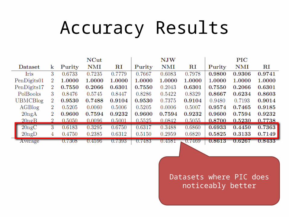
Accuracy Results
Datasets where PIC does noticeably better

Accuracy Results
Datasets where PIC does well, but Ncut and NJW fail completely

Accuracy Results
Datasets where PIC does well, but Ncut and NJW fail completely
Why? Isn’t PIC an one-dimension approximation to
Normalized Cut?

Why is PIC sometimes much better?
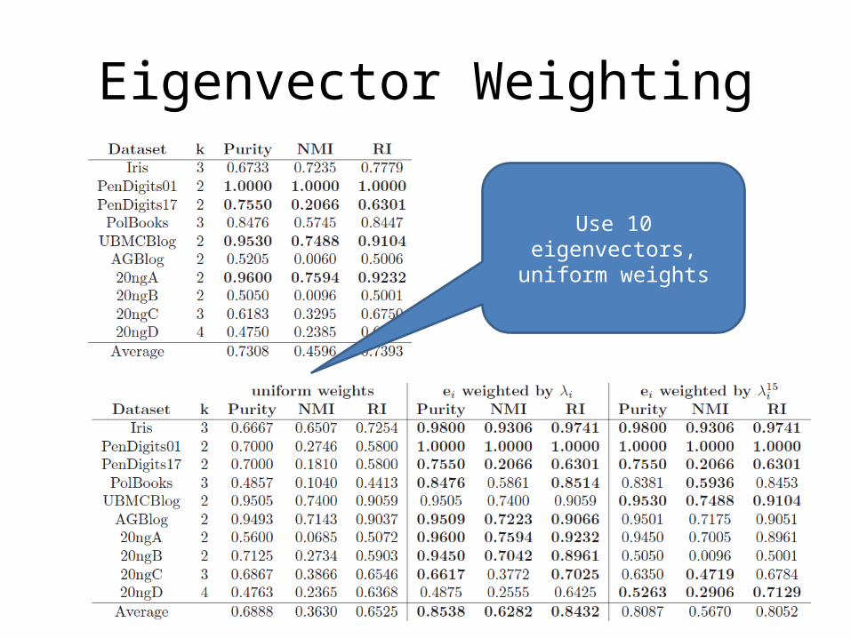
• To be precise, the embedding PIC provides is not just a linear combination of the top k eigenvectors; it is a linear combination of all the eigenvectors weighted exponentially by their respective eigenvalues.

Eigenvector Weighting
Original NCut – using k eigenvectors, uniform
weights on eigenvectors
Eigenvector Weighting
Use 10 eigenvectors, uniform weights

Eigenvector Weighting
Use 10 eigenvectors, weighted by respective
eigenvalues
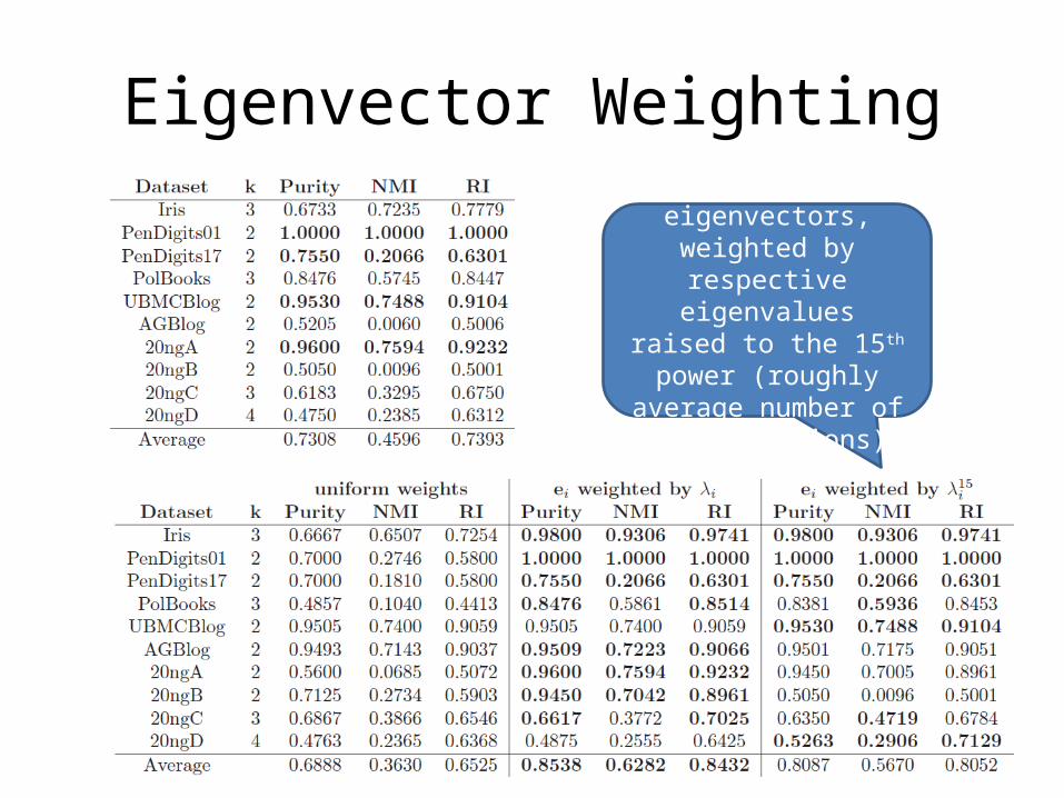
Eigenvector Weighting
Use 10 eigenvectors, weighted by respective
eigenvalues raised to the 15th power (roughly
average number of PIC iterations)

Eigenvector Weighting
Indiscriminant use of eigenvectors is bad – why original Normalized Cut
picks k

Eigenvector Weighting
Eigenvalue weighed NCut does much better than the original on these
datasets!

Eigenvector Weighting
Eigenvalue weighted NCut does much better than the original on these
datasets!
Exponentially eigenvalue weighted NCut does not do as well, but still much better than original
NCut

Eigenvector Weighting
• Eigenvalue weighting seems to improve results!• However, it requires a (possibly much) greater
number of eigenvectors and eigenvalues:– More eigenvectors may mean less precise
eigenvectors– It often means more computation time is required
• Eigenvector selection and weighting for spectral clustering is itself a subject of much recent study and research

PIC as a General Method

PIC as a General Method
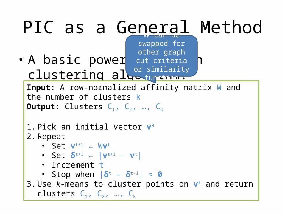
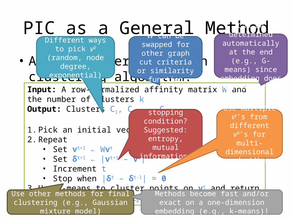
• A basic power iteration clustering algorithm:
Input: A row-normalized affinity matrix W and the number of clusters kOutput: Clusters C1, C2, …, Ck
1. Pick an initial vector v0
2. Repeat• Set vt+1 ← Wvt
• Set δt+1 ← |vt+1 – vt|• Increment t• Stop when |δt – δt-1| ≈ 0
3. Use k-means to cluster points on vt and return clusters C1, C2, …, Ck
PIC as a General Method
• A basic power iteration clustering algorithm:
Input: A row-normalized affinity matrix W and the number of clusters kOutput: Clusters C1, C2, …, Ck
1. Pick an initial vector v0
2. Repeat• Set vt+1 ← Wvt
• Set δt+1 ← |vt+1 – vt|• Increment t• Stop when |δt – δt-1| ≈ 0
3. Use k-means to cluster points on vt and return clusters C1, C2, …, Ck
W can be swapped for other graph cut criteria or similarity
function
Can be determined automatically at the end (e.g., G-means)
since embedding does not require k
Different ways to pick v0 (random, node
degree, exponential)
Better stopping condition?
Suggested: entropy, mutual information,
modularity, …
Use multiple vt’s from different v0’s
for multi-dimensional embedding
Use other methods for final clustering (e.g., Gaussian mixture model)
Methods become fast and/or exact on a one-dimension embedding (e.g., k-means)!

Spectral Clustering
• Things to consider:– Choosing a similarity function– Choosing the number of clusters k?– Which eigenvectors should be considered “significant”?
• The top or bottom k is not always the best for k clusters, especially on noisy data (Li et al. 2007, Xiang & Gong 2008)
– Finding eigenvectors and eigenvalues of a matrix is very slow in general: O(n3)
– Construction and storage of, and operations on a dense similarity matrix could be expensive: O(n2)

Large Scale Considerations
• But…what if the dataset is large and the similarity matrix is dense? For example, a large document collection where each data point is a term vector?
• Constructing, storing, and operating on an NxN dense matrix is very inefficient in time and space.

Lazy computation of distances and normalizers
• Recall PIC’s update is– vt = W*vt-1 = = D-1A * vt-1
– …where D is the [diagonal] degree matrix: D=A*1
• My favorite distance metric for text is length-normalized if-idf:– Def’n: A(i,j)=<vi,vj>/||vi||*||vj||
– Let N(i,i)=||vi|| … and N(i,j)=0 for i!=j
– Let F(i,k)=tf-idf weight of word wk in document vi
– Then: A = N-1FFTN-1

Large Scale Considerations
• Recall PIC’s update is– vt = W * vt-1 = = D-1A * vt-1
– …where D is the [diagonal] degree matrix: D=A*1– Let F(i,k)=TFIDF weight of word wk in document vi
– Compute N(i,i)=||vi|| … and N(i,j)=0 for i!=j
– Don’t compute A = N-1FFTN-1
– Let D(i,i)= N-1FFTN-1*1 where 1 is an all-1’s vector• Computed as D=N-1(F (FT (N-1*1))) for efficiency
– New update:• vt = D-1A * vt-1 = D-1 N-1FFTN-1 *vt-1

Experimental results• RCV1 text classification dataset– 800k + newswire stories– Category labels from industry vocabulary– Took single-label documents and categories with at least
500 instances– Result: 193,844 documents, 103 categories
• Generated 100 random category pairs– Each is all documents from two categories– Range in size and difficulty– Pick category 1, with m1 examples
– Pick category 2 such that 0.5m1<m2<2m1

Results
•NCUTevd: NCut using eigenvalue decomposition•NCUTiram: Implicit Restarted Arnoldi Method•No statistically significant difference between NCUTevd and PIC

Results

Results

Results
• Linear run-time implies constant number of iterations.
• Number of iterations to “acceleration-convergence” is hard to analyze:– Faster than a single complete run of power
iteration to convergence.– On our datasets• 10-20 iterations is typical• 30-35 is exceptional
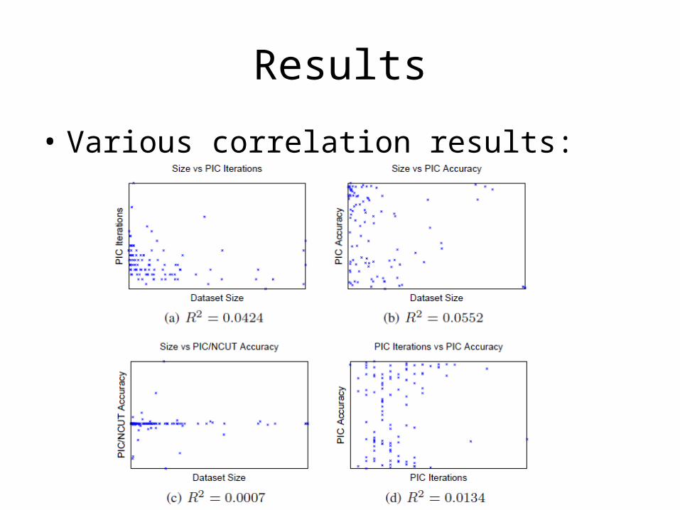
Results
• Various correlation results: