Embed Size (px)
Citation preview
Power Reduction Techniques for Networks-on-Chip
Amit Berman

Power Reduction Techniques for Networks-on-Chip
Research Thesis
Submitted in Partial Fulfillment of the Requirements for the Degree ofMaster of Science in Electrical Engineering
Amit Berman
Submitted to the Senate of the Technion - Israel Institute of Technology
SH’VAT, 5770 HAIFA FEBRUARY, 2010


The Research Thesis Was Done Under The Supervision of Prof. Idit Keidar
in the Department of Electrical Engineering.
I would like to thank Prof. Idit Keidar for the stimulating discussions, the
importent insights and the productive joint work.
I would like to thank Prof. Ran Ginosar for the joint research, for the
major contributions and unique point of view.
The Generous Financial Help of the Technion is Gratefully Acknowledged.

Contents
1 Introduction 5
1.1 Background: Networks-on-Chip . . . . . . . . . . . . . . . . . 5
1.2 Motivation: Power Consumption in Modern VLSI Systems . . 6
1.3 Structure and Contributions of this Thesis . . . . . . . . . . . 6
1.4 Related Work . . . . . . . . . . . . . . . . . . . . . . . . . . . 7
1.4.1 Interconnect Reliability . . . . . . . . . . . . . . . . . . 7
1.4.2 Power Consumption in NoC . . . . . . . . . . . . . . . 8
2 Parity Routing 11
2.1 Introduction . . . . . . . . . . . . . . . . . . . . . . . . . . . . 11
2.2 Goal and Definitions . . . . . . . . . . . . . . . . . . . . . . . 14
2.2.1 Problem Definition . . . . . . . . . . . . . . . . . . . . 14
2.2.2 Definitions . . . . . . . . . . . . . . . . . . . . . . . . . 16
2.3 Parity Routing Algorithm . . . . . . . . . . . . . . . . . . . . 17
2.3.1 PaR-1: One-bit Error Protection . . . . . . . . . . . . 17
2.3.2 PaR-r: r-bit Error Protection . . . . . . . . . . . . . . 18
2.4 Evaluation . . . . . . . . . . . . . . . . . . . . . . . . . . . . . 22
2.4.1 PaR-1 Analysis . . . . . . . . . . . . . . . . . . . . . . 23
2.4.2 PaR-r Analysis . . . . . . . . . . . . . . . . . . . . . . 25
2.4.3 Power Reduction Example . . . . . . . . . . . . . . . . 27
3 Selective Packet Interleaving 29
3.1 Introduction . . . . . . . . . . . . . . . . . . . . . . . . . . . . 29
3.2 Selective Packet Interleaving Algorithm . . . . . . . . . . . . . 31
3.3 Analysis . . . . . . . . . . . . . . . . . . . . . . . . . . . . . . 33
3.3.1 Assumptions . . . . . . . . . . . . . . . . . . . . . . . . 34
3.3.2 Case Analysis . . . . . . . . . . . . . . . . . . . . . . . 35
3.3.3 Typical Values and Comparison . . . . . . . . . . . . . 39
3.4 Benchmark Simulation . . . . . . . . . . . . . . . . . . . . . . 41
3.4.1 Methodology . . . . . . . . . . . . . . . . . . . . . . . 41
3.4.2 Simulation Results . . . . . . . . . . . . . . . . . . . . 42
3.4.3 Evaluation of Link and Interleaving Overhead . . . . . 43
3.5 Power Analysis . . . . . . . . . . . . . . . . . . . . . . . . . . 44
4 Conclusions 57
Appendices 59

List of Figures
2.1 Example: bit flip detection. . . . . . . . . . . . . . . . . . . . 13
2.2 Information flow among encoder, decoder and parity circuits. . 15
2.3 Node coordinates in a regular mesh. . . . . . . . . . . . . . . . 16
2.4 PaR-1 concept. . . . . . . . . . . . . . . . . . . . . . . . . . . 17
2.5 PaR-1 encoder pseudo-code. . . . . . . . . . . . . . . . . . . . 18
2.6 PaR-1 decoder pseudo-code. . . . . . . . . . . . . . . . . . . . 19
2.7 The 2r routing paths for r parity bits. . . . . . . . . . . . . . . 20
2.8 PaR-r encoder pseudo code. . . . . . . . . . . . . . . . . . . . 21
2.9 PaR-r decoder pseudo code. . . . . . . . . . . . . . . . . . . . 22
2.10 PaR cost reduction. . . . . . . . . . . . . . . . . . . . . . . . . 26
2.11 Example: PaR-1 power reduction. . . . . . . . . . . . . . . . . 28
3.1 Virtual channels (VCs) in a NoC router’s output buffer. . . . . 31
3.2 Example of SPI flit transmission scheme. . . . . . . . . . . . . 32
3.3 SPI flit selection with m virtual channels in a NoC router. . . 34
3.4 Expected values of the number of bit transitions. . . . . . . . 39
3.5 Percentage of reduction in the number of bit transitions. . . . 47

3.6 SPI vs. BI Comparison . . . . . . . . . . . . . . . . . . . . . . 48
3.7 Average number of bit transitions with various benchmarks. . 49
3.8 Simulated MP3 benchmark. . . . . . . . . . . . . . . . . . . . 50
3.9 Simulated values of the number of bit transitions. . . . . . . . 52
3.10 Simulated values of the number of bit transitions. . . . . . . . 54
3.11 SPI power reduction. . . . . . . . . . . . . . . . . . . . . . . . 55
1 PaR encoder hardware architecture. . . . . . . . . . . . . . . . 63
2 PaR decoder hardware architecture. . . . . . . . . . . . . . . . 64
3 SPI hardware architecture. . . . . . . . . . . . . . . . . . . . . 65
Abstract
Modern Network-on-Chip (NoC) links consume a significant fraction of the
total NoC power, e.g., one study has shown that they consume up to 60%
of total power and that this fraction is apparently growing. We present two
algorithms for power reduction in NoC links.
We first present Parity Routing (PaR), a novel method to add redundant
parity information to packets, while minimizing the number of redundant bits
transmitted. PaR exploits NoC path diversity in order to avoid transmitting
some of the redundant parity bits. Our analysis shows that, for example,
on a 4x4 NoC with a demand of one parity bit, PaR reduces the redundant
information transmitted by 75%, and the savings increase asymptotically to
100% with the size of the NoC. In addition, we show that PaR can yield
power savings due to the reduced number of bit transmissions. Furthermore,
PaR utilizes low complexity, small-area circuits.
Second, we present Selective Packet Interleaving (SPI), a flit transmission
scheme that reduces power consumption in NoC links. SPI decreases the
number of bit transitions in the links by exploiting the multiplicity of virtual
1

channels in a NoC router. SPI multiplexes flits to the router’s output link so
as to minimize the number of bit transitions from the previously transmitted
flit. Analysis and simulations demonstrate a reduction of up to 55% in the
number of bit transitions and up to 40% savings in power consumed on the
link. SPI benefits grow with the number of virtual channels. SPI works
better for links with a small number of bits in parallel. While SPI compares
favorably against bus inversion, combining both schemes helps to further
reduce bit transitions.
2

Symbols and Abbreviations
• VLSI - Very Large Scale Integration.
• FPGA - Field Programmable Gate Array.
• NoC - Network on Chip.
• VC - Virtual Channel.
• SPI - Selective Packet Interleaving.
• UC - Uncoded.
• BI - Bus Invert.
• SB - Combined Selective Packet Interleaving with Bus Invert.
• PaR-r - Parity Routing with r parity bits.
• ParVal(x) - Parity Value of variable x.
• dx(U, V ) - the vertical distance between nodes U and V.
• dy(U, V ) - the horizontal distance between nodes U and V.
3

• dd(U, V ) - the diagonal distance between nodes U and V.
• V = (Vx, Vy) - Vx and Vy are the coordinates of node V.
• orient(e) - orientation of the edge e, either horizontal or vertical.
• p[x] - parity bit in location x.
• dec2bin(x) - decimal to binary function on variable x.
• bin2dec(x) - binary to decimal function on variable x.
• CRx(N,M) - cost redcution of regular mesh NxM NoC using PaR-x.
• fi - Flit at the head of virtual channel number i.
• fLINK - Logic state of the NoC router’s output link.
• dH(p, q) - the Hamming distance between the flits fp and fq.
• Tx(n) - number of bit transitions from the previous state with x flit
transmission scheme.
4

Chapter 1
Introduction
1.1 Background: Networks-on-Chip
The Network-on-Chip (NoC) paradigm has evolved to replace ad-hoc global
wiring interconnects [7, 13, 14]. With this approach, system modules com-
municate by sending packets to one another over a network. The structured
NoC wiring allows for the use of high-performance circuits to reduce latency
and increase bandwidth [7, 13, 14].A conventional NoC consists of a packet-
switched network with a two-dimensional mesh topology [7, 36]. NoCs typi-
cally employ wormhole routing, i.e., each packet is divided into smaller units
called flits, which are forwarded individually on links [19, 36].
NoC routers typically employ multiple buffers, called virtual channels (VCs)
[26, 36, 44], which allows them to transmit several flows in parallel by inter-
leaving their flits on a single outgoing link. Currently proposed NoCs employ
5

between two and four VCs [19, 26], but studies argue that this number should
increase in future NoCs in order to supply higher throughput demands [36].
Each VC holds a buffer of flits pertaining to one flow.
1.2 Motivation: Power Consumption
in Modern VLSI Systems
Power consumption is becoming a crucial factor in the design of high-speed
digital systems, [1, 4, 5, 8, 12, 20, 21, 38, 44]. Whereas static power consump-
tion is due to leakage and short-circuit currents, dynamic power consumption
stems from switching activity, i.e., bit transitions. Interconnects consume the
lion’s share of dynamic power in modern chips. For example, studies show
that interconnect links consume up to 60% of the dynamic power in NoCs [1,
42], more than 60% of the dynamic power in a modern microprocessor [21],
and more than 90% in FPGA [15]. This portion is apparently growing [1, 9,
12, 33, 38, 44].
1.3 Structure and Contributions
of this Thesis
In this thesis, we address the challenge of reducing power consumption in NoC
links, in two contexts: coding for reliability (Chapter 2) and bus transitions
6

(Chapter 3).
The first problem we tackle in this thesis is to reduce the number of
redundant bit transmissions resulting from error detection [2]. A solution to
this problem is given in Chapter 2. Our analysis shows that, for example, on a
4x4 NoC with one redundant parity bit, our technique reduces the redundant
information transmitted by 75%, and the savings increase asymptotically to
100% with the size of the NoC.
Our second goal in this thesis is to develop an approach for reducing
the number of bit transitions in NoC interconnect links [3]. This problem is
tackled in Chapter 3. Analysis and simulations of our technique demonstrate
a reduction of up to 55% in the number of bit transitions and up to 40%
savings in power consumed on the link.
1.4 Related Work
1.4.1 Interconnect Reliability
Modern device scaling results in deep sub micron noises, which cause inter-
connect errors to be more dominant and harder to predict [10, 25, 27, 28, 29,
30, 41, 45], and also gives rise to new error sources [25, 27].
Traditional designs enhance interconnect reliability at the physical layer,
using worst-case design margins such as aggressive inter-wire spacing, inser-
tion of repeaters, and shielding of link wires [29, 32, 41]. Unfortunately, all
these techniques incur high area and power costs [27, 40]. Moreover, they
7

require knowledge of the circuit layout, thus inflicting design complexity [27,
30]. Furthermore, in novel technologies, the efficiency of these techniques
decreases because transient errors are becoming harder to predict [41].
A promising alternative to the traditional physical layer solutions is to add
reliability at the data-link layer of the NoC, using error detection codes, as
suggested in [30, 45]. Whereas error protection at the physical layer involves
circuit design techniques that rely on specific device parameters, data link
solutions are technology-independent [30].
In this thesis, we present a technique to save redundant bit transmissions
resulting from error detection codes, along with the associated power penalty.
1.4.2 Power Consumption in NoC
System-level power design approaches include synthesis algorithms to in-
crease the power efficiency in interconnection networks via better module
placement [15] or improved application design [23]. In such methods, the
traffic patterns among the cores need to be known a-priori. In contrast, the
approach we present in this thesis does not require a-priori knowledge of the
interconnect usage.
Embedded power design approaches include techniques for energy effi-
cient microarchitecture. For example, in [42] a power-driven design of router
for NoC is presented. The technique we present in this thesis can comple-
ment this approache, and combining both schemes can help to further reduce
power.
8
Data encoding is often employed to decrease the number of bit transitions
over interconnects. Popular methods include Bus Invert (BI) [38], adaptive
coding [16], gray coding [24] and transition method [35]. Of these, we elab-
orate only on BI, which was shown to be the most effective in NoCs [31]. BI
compares the data to be transmitted with the current data on link. If the
Hamming distance (the number of bits in which the data patterns differ) be-
tween the new information and the link state is larger than half the number
of bits (wires) on the link, then the data pattern is inverted before trans-
mission. To enable restoring the original data pattern, an extra control wire
is added to the link, in which a transmission of 1 indicates data inversion.
Analysis [37] shows that on link widths of more than 8 bits, the savings are
insufficient to justify the overhead of encoding circuits, and therefore wider
links are segmented.
Previous work [31] has investigated the reduction of NoC power consump-
tion achieved using the four mentioned data encoding schemes. Experiments
in 0.35µ technology showed that BI achieves the best results. We therefore
compare our technique to and combine our technique with BI in this thesis.
Nevertheless, the same paper found that the achieved power gain is offset by
the overhead required to implement the BI encoding scheme. In contrast, the
power savings achieved by our technique are higher than the power consumed
by the required overhead. The reasons for that are that our technique does
not add any redundant control wires.
Power may also be reduced using low-power device and circuit design tech-
9

niques, such as dynamic voltage and frequency scaling (DVFS) [17], which
adjust the supply voltage and clock rate dynamically according to circuit
parameters. The energy efficiency of DVFS is highly dependant on the slack
of the circuit. Another approach uses low-swing signaling techniques [13, 18,
43], the efficiency of which depends on circuit layout and manufacturing pa-
rameters. In contrast, the approach we present in this thesis does not require
knowledge about the circuit layout or manufacturing parameters.
10

Chapter 2
Parity Routing
2.1 Introduction
Modern device scaling results in deep sub micron noises, which cause inter-
connect errors to be more dominant and harder to predict [10, 25, 27, 28,
29, 30, 41, 45], and also gives rise to new error sources [25, 27]. The need for
efficient low-power design techniques, along with aggressive voltage scaling
and higher integration make interconnects even more susceptible to errors
[10, 30, 45]. In this chapter, we focus on efficient solutions for interconnect
reliability in the context of NoCs. Our goal is to provide any desired level of
error detection, while reducing the number of redundant bits, as we specify
in Section 2.2.
In Section 2.3, we present Parity Routing (PaR), a novel method for error
protection in NoC. The main idea behind our approach is to take advantage of
11

the multiplicity of routing paths between nodes. Path diversity was exploited
in the past in order to achieve load-balancing, by routing some traffic XY
and remaining traffic YX [39]. Here, we use it for the first time for error
detection, and achieve better load balancing as a favorable side effect of
this approach. For example, if one bit error detection is required, then the
traditional approach is to add a single parity bit to the packet. In PaR,
we save the redundant bit by selecting the routing path according to the
parity of the data. As in [30], errors are detected at every hop: routers
along the path can identify parity errors by observing that the packet is on
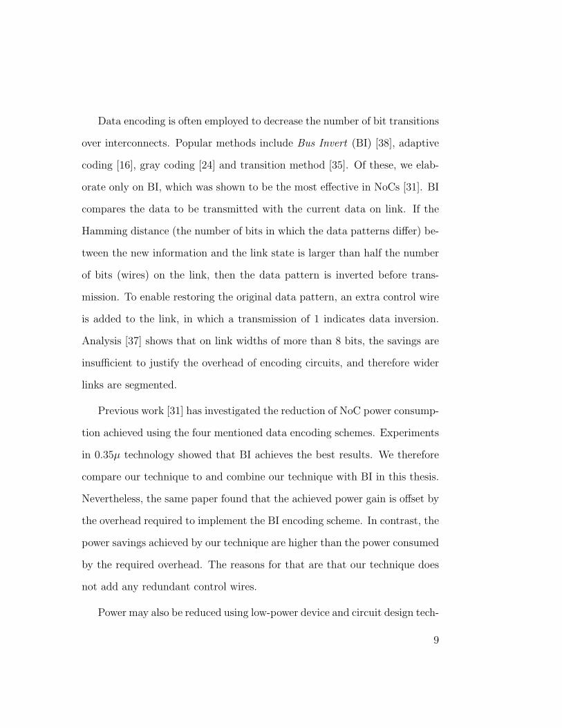
the wrong path. We illustrate this in Fig. 2.1, where a packet is transferred
from a source node, S, to a destination node, D, on a regular mesh NoC.
The data parity determines the routing path: 0 for XY routing and 1 for
YX. In Fig. 2.1, the data is 0101, so the parity bit is 0, which indicates XY
routing. While transferring the packet from S to the adjacent horizontal node
(according to XY routing), one error occurs, changing the data to 0111. At
the receiving node, the calculated parity bit is then 1, which indicates YX
routing. Since the edge the packet arrives on is not on the expected path, an
error is deduced.
A single parity bit can be saved whenever there are more than two avail-
able paths between the source and destination nodes. However, this may not
always be the case if we wish to employ shortest-path routing: if the source
and the destination nodes share one coordinate (either X or Y) there is only
one shortest routing path. In such cases, PaR adds an extra parity bit to the
12
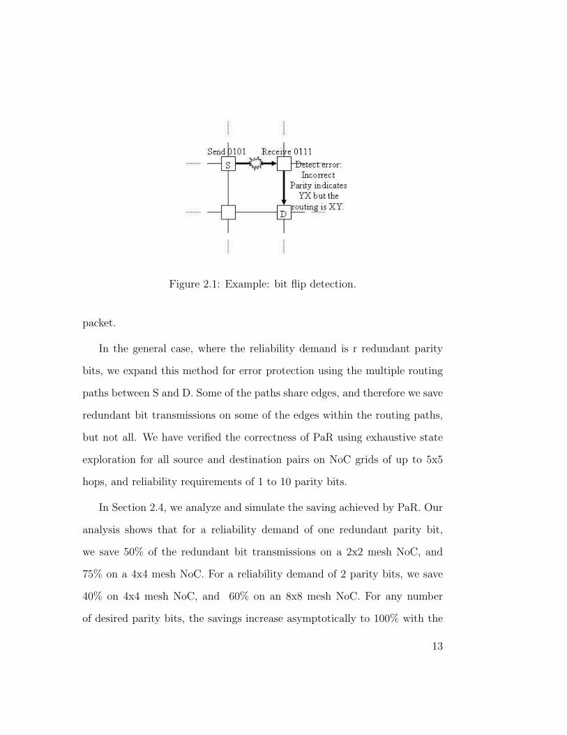
Figure 2.1: Example: bit flip detection.
packet.
In the general case, where the reliability demand is r redundant parity
bits, we expand this method for error protection using the multiple routing
paths between S and D. Some of the paths share edges, and therefore we save
redundant bit transmissions on some of the edges within the routing paths,
but not all. We have verified the correctness of PaR using exhaustive state
exploration for all source and destination pairs on NoC grids of up to 5x5
hops, and reliability requirements of 1 to 10 parity bits.
In Section 2.4, we analyze and simulate the saving achieved by PaR. Our
analysis shows that for a reliability demand of one redundant parity bit,
we save 50% of the redundant bit transmissions on a 2x2 mesh NoC, and
75% on a 4x4 mesh NoC. For a reliability demand of 2 parity bits, we save
40% on 4x4 mesh NoC, and 60% on an 8x8 mesh NoC. For any number
of desired parity bits, the savings increase asymptotically to 100% with the
13

size of the network. In addition, PaR can yield power saving as it saves bit
transmissions and simplifies the error detection decoding process.
2.2 Goal and Definitions
We tackle the problem of hop by hop error detection. The required reliability
level is expressed as the number r, of redundant bits. An externally provided
function (or circuit), parity(data), returns r parity bits for protecting data.
Any parity function can be used, e.g., CRC [28]. We denote the r redundant
parity bits as p[1],p[2],...,p[r].
2.2.1 Problem Definition
Our goal is to design an error detection algorithm, which reduces the trans-
mission of redundant bits, yet with low encoder and decoder circuit overheads
and a low design complexity. Consider a packet sent from a source node S
to a destination node D, in a regular mesh NoC. We require that the routing
from S to D will be on one of the shortest paths. A Coding solution consists
of two components, an encoder and a decoder. The encoder and decoder
circuits are placed at each node, providing hop-by-hop error detection. We
denote the current node where encoding/decoding occurs as H. The encoder
and decoder’s functions are defined as follows:
1. Encoder: Given H, S, D, and the packet’s data, the encoder decides
which edge is next on the packet’s routing path, and whether there is
14
a need to add redundant parity bits to the packet.
2. Decoder: Given H, S, D, the packet, and the incoming edge, the decoder
determines whether an error had occurred.
The flow of information among the different components is shown in Fig. 2.2.
We denote concatenation by commas, e.g., data,p[1] represents the data
with one parity bit appended at the end. If pack=data,p[1] then we denote
data=pack-p[1].
Figure 2.2: Information flow among encoder, decoder and parity circuits.
Note that since the encoder determines the routing path, this approach
is applicable for transmission units that carry the source and destination
addresses. In case the NoC employs wormhole routing [1], typically only
the header flit carries these addresses. In such cases, our scheme can be
used for the header flit, which is the most important flit. In other non-
wormhole routing schemes, this approach is applicable for the entire packet
(with checking at the destination node) .For the remainder of this chapter,
we simply refer to the protected transmission unit as a packet.
15
2.2.2 Definitions
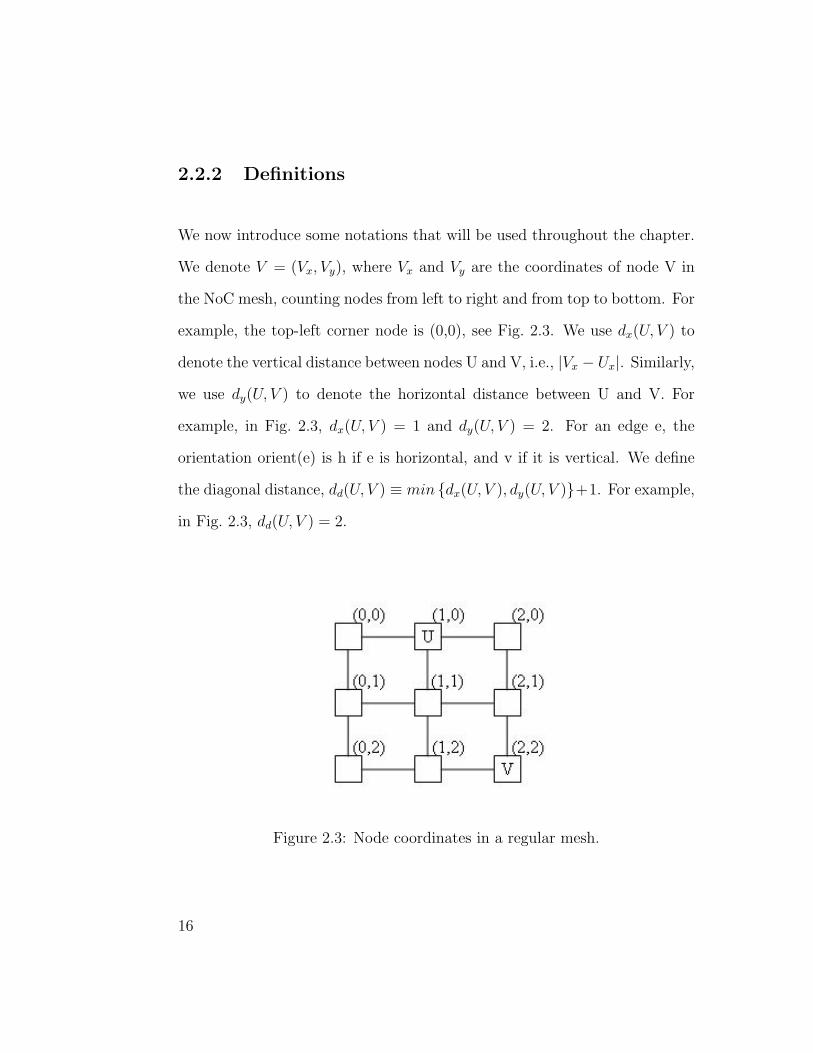
We now introduce some notations that will be used throughout the chapter.
We denote V = (Vx, Vy), where Vx and Vy are the coordinates of node V in
the NoC mesh, counting nodes from left to right and from top to bottom. For
example, the top-left corner node is (0,0), see Fig. 2.3. We use dx(U, V ) to
denote the vertical distance between nodes U and V, i.e., |Vx − Ux|. Similarly,
we use dy(U, V ) to denote the horizontal distance between U and V. For
example, in Fig. 2.3, dx(U, V ) = 1 and dy(U, V ) = 2. For an edge e, the
orientation orient(e) is h if e is horizontal, and v if it is vertical. We define
the diagonal distance, dd(U, V ) ≡ min {dx(U, V ), dy(U, V )}+1. For example,
in Fig. 2.3, dd(U, V ) = 2.
Figure 2.3: Node coordinates in a regular mesh.
16

2.3 Parity Routing Algorithm
In this section, we develop the PaR algorithm. For clarity of the exposition,
we first present the special case of a reliability demand of one parity bit,
called PaR-1, and then expand the algorithm for r redundant parity bits.
We prove the correctness of the PaR algorithm in the appendices.
2.3.1 PaR-1: One-bit Error Protection
Consider the case of a reliability demand of one bit error detection. We use
the given parity function to calculate the parity bit of the packet. If the
parity bit is 0, PaR-1 routes the packet XY, and in case the parity bit is 1,
the routing is YX, as shown in Fig. 2.4. If S and D are located on the same
row or column, then the parity bit is sent along with the packet.
The pseudo-code of PaR-1 encoder is shown in Fig. 2.5.
Figure 2.4: PaR-1 concept.
17

(1) PaR-1 Encode (H, S, D, data)(2) if (H = D) then return data, no next hop(3) next hop ← next hop on XY route to D(4) packet ← data(5) p[1] ← parity(data, S, D)(6) if (Sx = Dx) or (Sy = Dy) then packet ← data,p[1](7) else if (p[1] = 1) then next hop ← next hop on YX route to D(8) return packet, next hop
Figure 2.5: PaR-1 encoder pseudo-code.
The pseudo-code of PaR-1 decoder is shown in Fig. 2.6.
The property that allows us to detect the parity bits according to the
routing path is the fact that the XY and YX paths between every S and D
that do not share a coordinate are edge-disjoint.
2.3.2 PaR-r: r-bit Error Protection
Generally speaking, in order to provide a detection level of r-parity bits
without sending redundant bits, we need to distinguish between 2r edge-
disjoint routing paths. Since there are at most 2 edge-disjoint paths between
every pair of nodes, PaR-r strives to achieve disjointedness on as many edges
as possible, by choosing paths with minimal overlap. For example, in Fig. 2.7,
we see an example of the 2r routing paths PaR-r uses between S and D for
the different values of the r parity bits.
First, note that there aren’t always 2r different shortest paths: if S and D
18
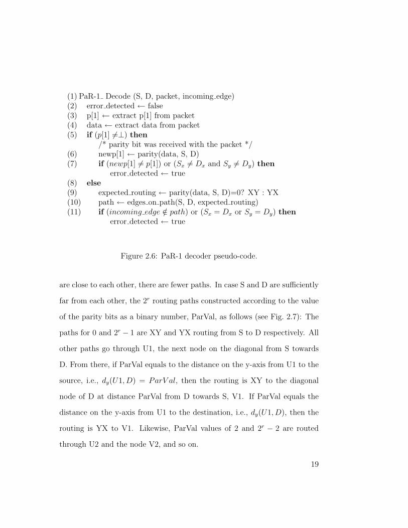
(1) PaR-1 Decode (S, D, packet, incoming edge)(2) error detected ← false(3) p[1] ← extract p[1] from packet(4) data ← extract data from packet(5) if (p[1] 6=⊥) then
/* parity bit was received with the packet */(6) newp[1] ← parity(data, S, D)(7) if (newp[1] 6= p[1]) or (Sx 6= Dx and Sy 6= Dy) then
error detected ← true(8) else(9) expected routing ← parity(data, S, D)=0? XY : YX(10) path ← edges on path(S, D, expected routing)(11) if (incoming edge /∈ path) or (Sx = Dx or Sy = Dy) then
error detected ← true
Figure 2.6: PaR-1 decoder pseudo-code.
are close to each other, there are fewer paths. In case S and D are sufficiently
far from each other, the 2r routing paths constructed according to the value
of the parity bits as a binary number, ParVal, as follows (see Fig. 2.7): The
paths for 0 and 2r − 1 are XY and YX routing from S to D respectively. All
other paths go through U1, the next node on the diagonal from S towards
D. From there, if ParVal equals to the distance on the y-axis from U1 to the
source, i.e., dy(U1, D) = ParV al, then the routing is XY to the diagonal
node of D at distance ParVal from D towards S, V1. If ParVal equals the
distance on the y-axis from U1 to the destination, i.e., dy(U1, D), then the
routing is YX to V1. Likewise, ParVal values of 2 and 2r − 2 are routed
through U2 and the node V2, and so on.
19
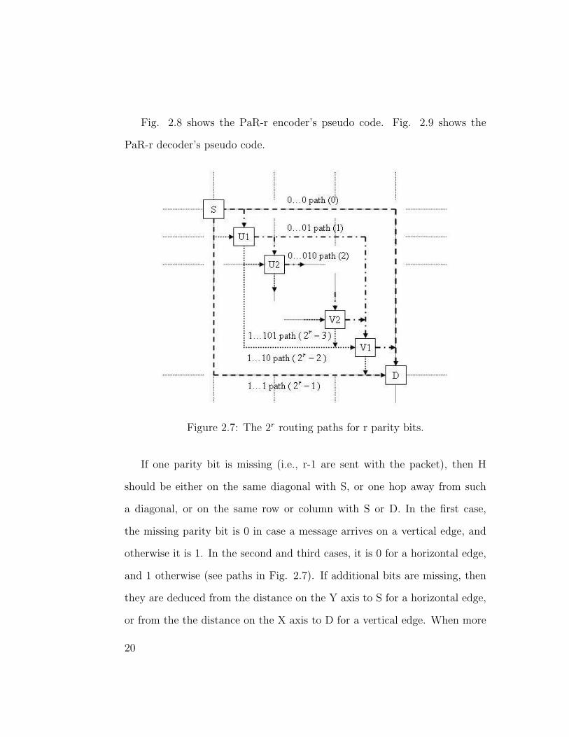
Fig. 2.8 shows the PaR-r encoder’s pseudo code. Fig. 2.9 shows the
PaR-r decoder’s pseudo code.
Figure 2.7: The 2r routing paths for r parity bits.
If one parity bit is missing (i.e., r-1 are sent with the packet), then H
should be either on the same diagonal with S, or one hop away from such
a diagonal, or on the same row or column with S or D. In the first case,
the missing parity bit is 0 in case a message arrives on a vertical edge, and
otherwise it is 1. In the second and third cases, it is 0 for a horizontal edge,
and 1 otherwise (see paths in Fig. 2.7). If additional bits are missing, then
they are deduced from the distance on the Y axis to S for a horizontal edge,
or from the the distance on the X axis to D for a vertical edge. When more
20
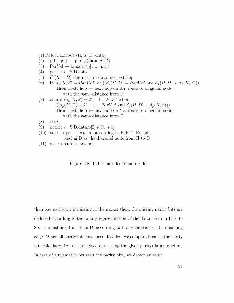
(1) PaR-r Encode (H, S, D, data)(2) p[1]...p[r] ← parity(data, S, D)(3) ParVal ← bin2dec(p[1],...,p[r])(4) packet ← S,D,data(5) if (H = D) then return data, no next hop(6) if (dy(H,S) = ParV al) or ((dx(H,D) = ParV al and dx(H,D) < dx(H,S)))
then next hop ← next hop on XY route to diagonal nodewith the same distance from D
(7) else if (dx(H,S) = 2r − 1− ParV al) or((dy(H,D) = 2r − 1− ParV al and dy(H,D) < dy(H,S)))then next hop ← next hop on YX route to diagonal node
with the same distance from D(8) else(9) packet ← S,D,data,p[2],p[3]...p[r](10) next hop ← next hop according to PaR-1 Encode
placing D as the diagonal node from H to D(11) return packet,next hop
Figure 2.8: PaR-r encoder pseudo code.
than one parity bit is missing in the packet then, the missing parity bits are
deduced according to the binary representation of the distance from H or to
S or the distance from H to D, according to the orientation of the incoming
edge. When all parity bits have been decoded, we compare them to the parity
bits calculated from the received data using the given parity(data) function.
In case of a mismatch between the parity bits, we detect an error.
21
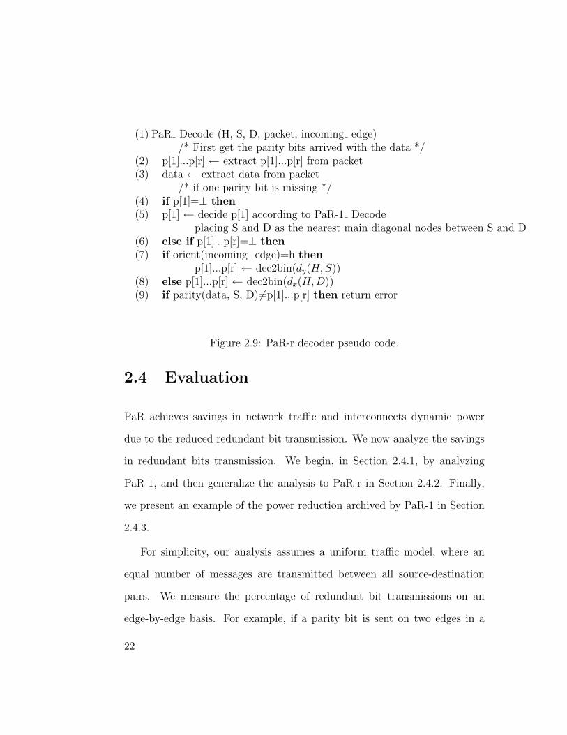
(1) PaR Decode (H, S, D, packet, incoming edge)/* First get the parity bits arrived with the data */
(2) p[1]...p[r] ← extract p[1]...p[r] from packet(3) data ← extract data from packet
/* if one parity bit is missing */(4) if p[1]=⊥ then(5) p[1] ← decide p[1] according to PaR-1 Decode
placing S and D as the nearest main diagonal nodes between S and D(6) else if p[1]...p[r]=⊥ then(7) if orient(incoming edge)=h then
p[1]...p[r] ← dec2bin(dy(H,S))(8) else p[1]...p[r] ← dec2bin(dx(H,D))(9) if parity(data, S, D) 6=p[1]...p[r] then return error
Figure 2.9: PaR-r decoder pseudo code.
2.4 Evaluation
PaR achieves savings in network traffic and interconnects dynamic power
due to the reduced redundant bit transmission. We now analyze the savings
in redundant bits transmission. We begin, in Section 2.4.1, by analyzing
PaR-1, and then generalize the analysis to PaR-r in Section 2.4.2. Finally,
we present an example of the power reduction archived by PaR-1 in Section
2.4.3.
For simplicity, our analysis assumes a uniform traffic model, where an
equal number of messages are transmitted between all source-destination
pairs. We measure the percentage of redundant bit transmissions on an
edge-by-edge basis. For example, if a parity bit is sent on two edges in a
22

four-hop path, the savings on this path are 50analyze the average savings
over all paths.
2.4.1 PaR-1 Analysis
Consider an NxM regular NoC mesh with NM nodes. The number of po-
tential source-destination (S-D) pairs in the NoC is NM(NM-1). Each of the
NM nodes has N-1 potential destinations that share the Y coordinate with
it. Thus, there are (N-1)NM S-D pairs that share this coordinate. Similarly,
there are (M-1)NM S-D pairs that share the X coordinate. The number of
S-D pairs between which the transmission of the parity bit is saved is:
NM(NM − 1)− (N − 1)NM − (M − 1)NM = (NM −N −M + 1)NM
We next compute the percentage of savings in terms of edges. The aver-
age path length when S and D share the Y coordinate is N+13
. In a similar
way, the average path length when S and D share x coordinate is M+13
. When
S and D are not on same axis, the average path length is N+M+23
. Denote by
CR1(N,M) the percentage of edges on the paths between all the S-D pairs for
which the redundant bit is not sent by PaR-1, on an NxM NoC mesh. We get:
CR1(N,M) = 1− (N + 1)(N − 1) + (M + 1)(M − 1)
(N + 1)(N − 1) + (M + 1)(M − 1) + (NM −N −M + 1)(N +M + 2)
In case the network is symmetric, i.e., N=M, we get:
23
CR1(N,M) = 1− 2(N + 1)(N − 1)
2(N + 1)(N − 1) + 2(N + 1)(N − 1)2=N − 1
N
For example, in case of a 4x4 network, the cost reduction is 75% of the
redundancy bits. We observe that as we increase the network (in both di-
mensions equally) the CR1 grows to 100%:
limN→∞
CR1(N,N) = 1
Similarly, for rectangles with any constant ratio, α, between the width
and length, where M = αN this observation is also valid.
In order to show this, we simplify the analysis and prove that the percent-
age of paths on which no parity bits are sent is asymptotically zero. Since
these paths are, on average, shorter than paths where parity bits are sent (as
shown above), this simpler result implies that the savings increase asymp-
totically to 100%. We observe that the percentage of pairs for which we save
the redundant bit transmissions is:
limN→∞
CR1(N,αN) = 1.
24
2.4.2 PaR-r Analysis
We now analyze the general case of r parity bits, PaR-r. Consider an NxM
NoC, a reliability demand of r redundant bits, and two given nodes S and D.
Without using the PaR algorithm, we have to transmit r redundant parity
bits on all edges in the path, that is, on dx(S,D) + dy(S,D) edges. Assume
that PaR-r can transmit the packet without the redundant r parity bits, i.e.,
blog2(dd(S,D))c ≥ r. According to the PaR-r algorithm, the amount of re-
dundant parity bits depends on the value of the parity bits (ParVal). There
are 2 routing paths (0 and 2r − 1) on which no redundant bits are sent on
any edge. There are 2 routing paths (1 and 2r − 2) on which there are r− 1
redundant bits sent on 4 edges. For ParVals of 2 and 2r−3, there are (r−1)
redundant parity bits transmitted on 8 edges (first 4 from S and last 4 to D)
and so on, until (r − 1) redundant parity bits are transmitted for a ParVal
of (2r − 1). Assuming that ParVal is distributed uniformly, the average re-
dundant parity bits transmitted from S to D is therefore:
(r − 1)2[0 + 4 + ...+ 4(2r − 1)
2r(dx(S,D) + dy(S,D))=
2(r − 1)(2r−1 − 1)
dx(S,D) + dy(S,D)
It is easy to see, that as the NoC grows, the percentage of S-D pairs for
which PaR-r can choose 2r paths asymptotically grows to 100%. For such
pairs, the average value of the denominator in the equation above (averaging
over all relevant S-D pairs) grows to infinity with the NoC size, while the
nominator remains constant. Hence, the percentage of parity bits actually
25
transmitted goes asymptotically to zero. In other word, for any constant r,
the savings of PaR-r grow asymptotically to 100% with the size of the NoC.
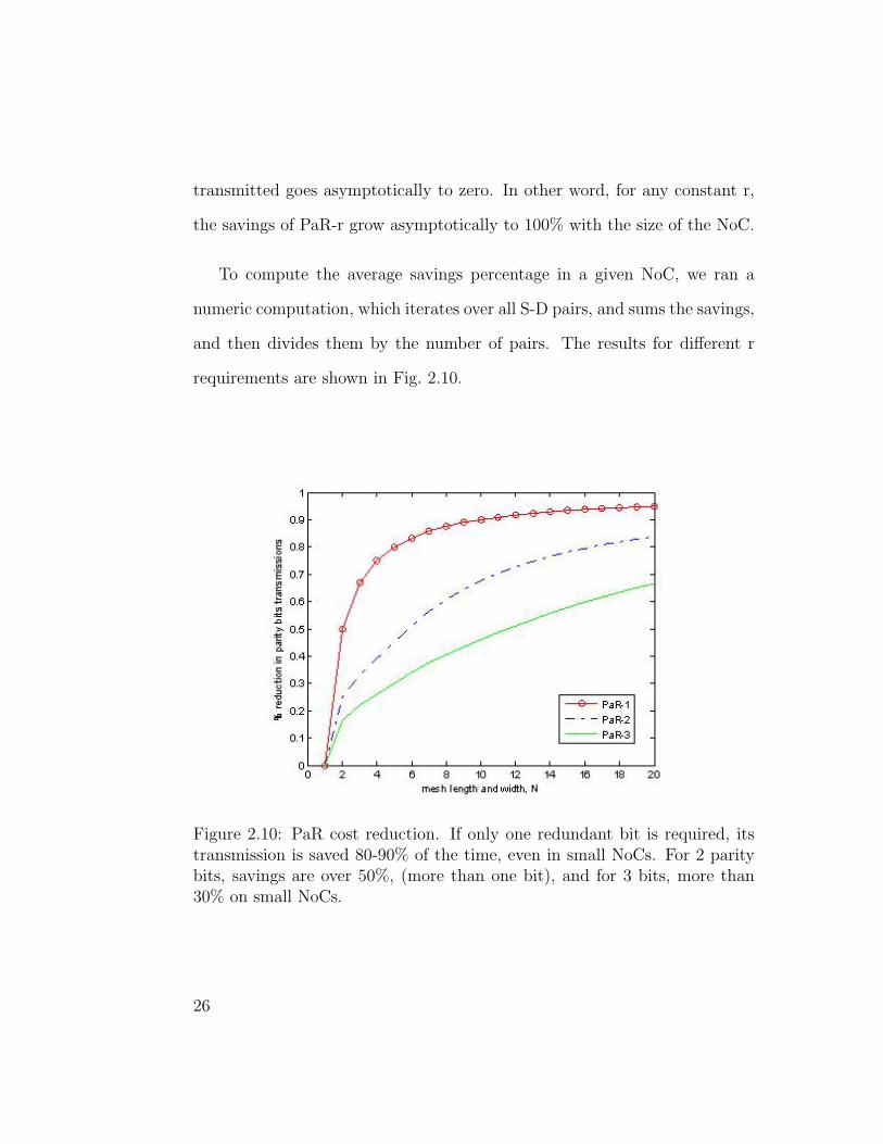
To compute the average savings percentage in a given NoC, we ran a
numeric computation, which iterates over all S-D pairs, and sums the savings,
and then divides them by the number of pairs. The results for different r
requirements are shown in Fig. 2.10.
Figure 2.10: PaR cost reduction. If only one redundant bit is required, itstransmission is saved 80-90% of the time, even in small NoCs. For 2 paritybits, savings are over 50%, (more than one bit), and for 3 bits, more than30% on small NoCs.
26

2.4.3 Power Reduction Example
We demonstrate the power saving achieved by PaR-1 with NxN regular mesh
NoC with 5mm long, 8-bit width links. Hardware design is implemented on
0.18µ TOWER process, and synthesized by Synopsis’s design compiler. In-
terconnect power consumption is measured by SPICE model, assume random
data and traffic patterns. Hardware architecture scheme is described at the
appendices.
Measurements of the redundant bits switching power, along with the par-
ity circuits’ power and PaR circuits’ power are referred as power consumption
and shown at Fig. 2.11. The measurements were made on 2x2, 3x3 and 4x4
regular mesh NoCs. We can observe increased power saving with the size of
the NoC. We expect the savings to grow as more parity bits are used because
of less redundant network traffic.
27
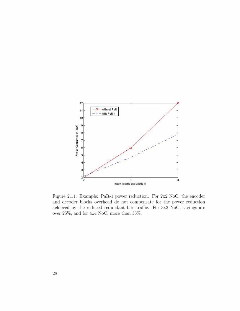
Figure 2.11: Example: PaR-1 power reduction. For 2x2 NoC, the encoderand decoder blocks overhead do not compensate for the power reductionachieved by the reduced redundant bits traffic. For 3x3 NoC, savings areover 25%, and for 4x4 NoC, more than 35%.
28
Chapter 3
Selective Packet Interleaving
3.1 Introduction
NoC links consume a significant fraction of the total NoC power [1, 5, 42]. We
present Selective Packet Interleaving (SPI), a new flit transmission scheme for
NoC-based systems. SPI reduces the dynamic power consumption on NoC
links by reducing the number of bit transitions. SPI assumes that the NoC
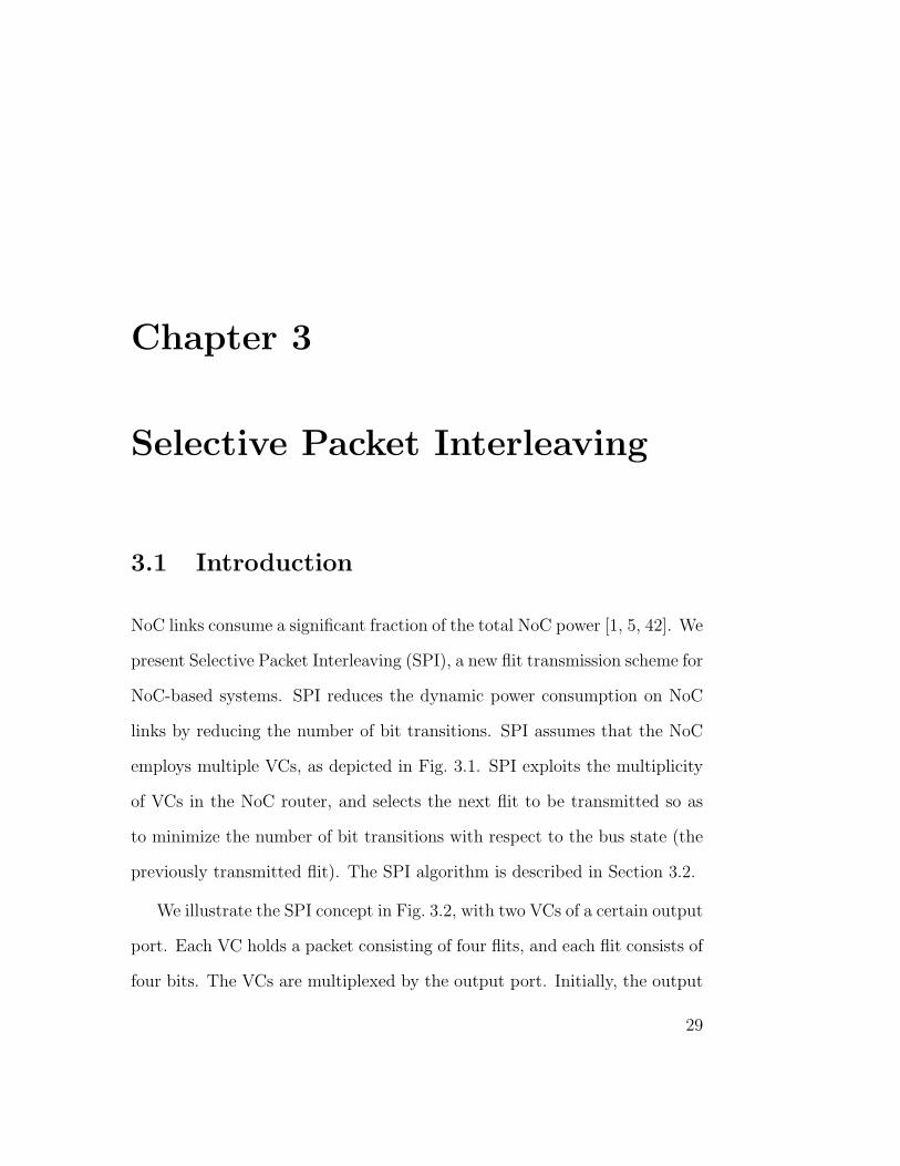
employs multiple VCs, as depicted in Fig. 3.1. SPI exploits the multiplicity
of VCs in the NoC router, and selects the next flit to be transmitted so as
to minimize the number of bit transitions with respect to the bus state (the
previously transmitted flit). The SPI algorithm is described in Section 3.2.
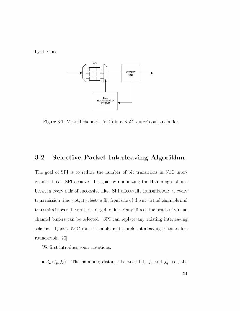
We illustrate the SPI concept in Fig. 3.2, with two VCs of a certain output
port. Each VC holds a packet consisting of four flits, and each flit consists of
four bits. The VCs are multiplexed by the output port. Initially, the output
29

is 0110. The output port can then select either flit 1001 of VC1 or flit 1110
from VC2. Selecting 1001 results in four bit transitions on the output link
relative to the previously transmitted flit, whereas selecting of 1110 results
in only one bit transition. Therefore, the output port selects the 1110 flit,
according to SPI.
SPI complements low-power design techniques such as voltage scaling,
and can be implemented on top of such methods. In contrast to these ap-
proaches, SPI is technology-independent. Similarly, SPI is orthogonal to
system-level design optimizations such as power-aware module placement,
and unlike them, SPI does not require any a priori knowledge of the inter-
connect traffic patterns. Thus, SPI is broadly applicable, and can co-exist
with a range of additional power optimizations.
In Section 3.3, we analyze the expected number of bit transitions with
SPI and compare it to three other flit transmission schemes. Our results
show that SPI can reduce the number of bit transitions by up to 55%. SPI’s
benefits grow with the number of virtual channels. In Section 3.4, we simulate
SPI with benchmarks as used in [31]. We then validate the analysis results
with the benchmark simulation results, and observe that the reduction in the
number of bit transitions is similar for different benchmark workloads.
Finally, in Section 3.5, we synthesize SPI with VLSI design tools, and de-
rive the resulting power reduction using place and route design automation
tools mapped to the Tower Semiconductor 0.18µ process library. Power anal-
ysis results show that SPI can yield up to 40% savings in power consumed
30
by the link.
Figure 3.1: Virtual channels (VCs) in a NoC router’s output buffer.
3.2 Selective Packet Interleaving Algorithm
The goal of SPI is to reduce the number of bit transitions in NoC inter-
connect links. SPI achieves this goal by minimizing the Hamming distance
between every pair of successive flits. SPI affects flit transmission: at every
transmission time slot, it selects a flit from one of the m virtual channels and
transmits it over the router’s outgoing link. Only flits at the heads of virtual
channel buffers can be selected. SPI can replace any existing interleaving
scheme. Typical NoC router’s implement simple interleaving schemes like
round-robin [20].
We first introduce some notations.
• dH(fp, fq) - The hamming distance between flits fp and fq, i.e., the
31
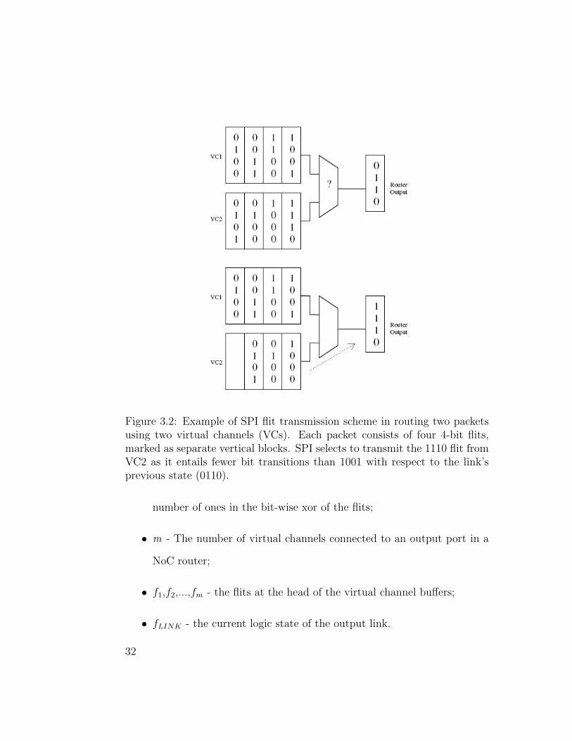
Figure 3.2: Example of SPI flit transmission scheme in routing two packetsusing two virtual channels (VCs). Each packet consists of four 4-bit flits,marked as separate vertical blocks. SPI selects to transmit the 1110 flit fromVC2 as it entails fewer bit transitions than 1001 with respect to the link’sprevious state (0110).
number of ones in the bit-wise xor of the flits;
• m - The number of virtual channels connected to an output port in a
NoC router;
• f1,f2,...,fm - the flits at the head of the virtual channel buffers;
• fLINK - the current logic state of the output link.
32
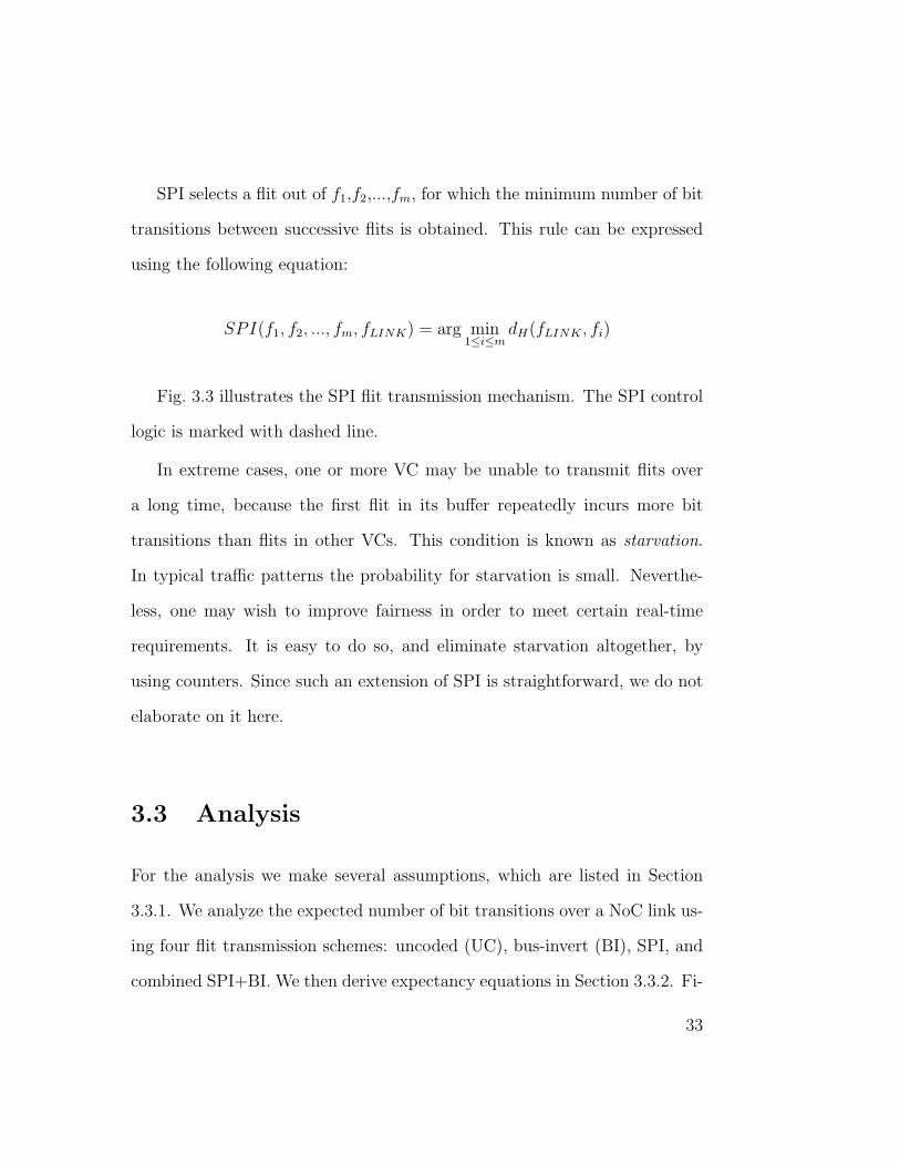
SPI selects a flit out of f1,f2,...,fm, for which the minimum number of bit
transitions between successive flits is obtained. This rule can be expressed
using the following equation:
SPI(f1, f2, ..., fm, fLINK) = arg min1≤i≤m
dH(fLINK , fi)
Fig. 3.3 illustrates the SPI flit transmission mechanism. The SPI control
logic is marked with dashed line.
In extreme cases, one or more VC may be unable to transmit flits over
a long time, because the first flit in its buffer repeatedly incurs more bit
transitions than flits in other VCs. This condition is known as starvation.
In typical traffic patterns the probability for starvation is small. Neverthe-
less, one may wish to improve fairness in order to meet certain real-time
requirements. It is easy to do so, and eliminate starvation altogether, by
using counters. Since such an extension of SPI is straightforward, we do not
elaborate on it here.
3.3 Analysis
For the analysis we make several assumptions, which are listed in Section
3.3.1. We analyze the expected number of bit transitions over a NoC link us-
ing four flit transmission schemes: uncoded (UC), bus-invert (BI), SPI, and
combined SPI+BI. We then derive expectancy equations in Section 3.3.2. Fi-
33
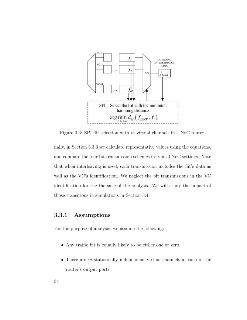
Figure 3.3: SPI flit selection with m virtual channels in a NoC router.
nally, in Section 3.3.3 we calculate representative values using the equations,
and compare the four bit transmission schemes in typical NoC settings. Note
that when interleaving is used, each transmission includes the flit’s data as
well as the VC’s identification. We neglect the bit transmissions in the VC
identification for the the sake of the analysis. We will study the impact of
those transitions in simulations in Section 3.4.
3.3.1 Assumptions
For the purpose of analysis, we assume the following:
• Any traffic bit is equally likely to be either one or zero.
• There are m statistically independent virtual channels at each of the
router’s output ports.
34
• Flit size and link width are equal, i.e., have the same number of bits,
n, which is assumed an even number.
3.3.2 Case Analysis
We analyze the expected number of bit transitions in the UC, BI, SPI and
combined SPI+BI flit transmission schemes. In the transmission of a single
random n-bit flit, the following random variables capture the number of bit
transitions from the previous state for the four schemes, over links of width
n and with m virtual channels:
• TUC(n) - uncoded, non-interleaved transmission.
• TBI(n) - bus invert transmission.
• TSPI(n) - SPI transmission.
• TSB(n) - SPI+BI transmission.
1. UC Uncoded and non-interleaved
In uncoded transmissions, the number of bit transitions per flit is dis-
tributed binomially with n tries and p=1/2. Hence, the expected num-
ber of transitions is:
E [TUC(n)] =n
2
35
2. BI - Bus-Invert
The link width for bus invert is n+1. For any k, 0 ≤ k ≤ n/2, the
probability for exactly k bit transitions out of the n+1 bits on the link
is:
P [TBI(n) = k] =
(n+ 1
k
)1
2n+1+
(n+ 1
n+ 1− k
)1
2n+1=
=
(n+ 1
k
)1
2n
The expected number of transitions is thus:
E [TBI(n)] =
n/2∑k=0
Pr [TBI(n) = k] · k =
=
n/2∑k=0
(n+ 1
k
)k
2n
3. SPI - Selective Packet Interleaving
We now consider SPI. The random variable V Ci captures the incurred
number of bit transitions if the first flit in virtual channel number i is
transmitted on the output link. V Ci is the Hamming distance between
the first flit in the buffer of VC number i and the output link. Note
that by assumption, all V Ci s are identically distributed. For any m
virtual channels, 1 ≤ m, and for any k, 0 ≤ k ≤ n, the probability for
36

exactly k bit transitions out of the n bits on the link is:
Pr [TSPI(n,m) = k] = Pr [min {V C1, V C2, ..., V Cm} = k] =
= Pr [V C1 = k, V C2 > k, ..., V Cm > k] +
+ Pr [V C1 > k, V C2 = k, ..., V Cm > k] + ...+
+ Pr [V C1 > k, V C2 > k, ..., V Cm = k] +
+ Pr [V C1 = k, V C2 = k, ..., V Cm > k] + ...+
+ Pr [V C1 = k, V C2 = k, ..., V Cm = k] =
=
(m
1
)[(n
k
)1
2n
]1[
n∑i=k+1
(n
i
)1
2n
](m−1)
+ ...+
+
(m
m
)[(n
k
)1
2n
]m[
n∑i=k+1
(n
i
)1
2n
]0
=
=m∑
i=1
(m
i
)[(n
k
)1
2n
]i[
n∑j=k+1
(n
j
)1
2n
](m−i)
=
=1
2nm
m∑i=1
(m
i
)(n
k
)i[
n∑j=k+1
(n
j
)](m−i)
The expected number of transitions is thus:
E [TSPI(n,m)] =n∑
k=0
Pr [TSPI(n,m) = k] · k =
=1
2nm
n∑k=0
m∑i=1
(m
i
)(n
k
)i[
n∑j=k+1
(n
j
)](m−i) k
37

4. SPI + Bus-Invert
As for BI, the link width for the combined SPI+BI scheme is also n+1.
Similar to SPI, V Ci captures the incurred number of bit transitions if
the head of queue flit in virtual channel number i is transmitted on the
output link, using BI. For any m virtual channels, 1 ≤ m, and for any
k, 0 ≤ k ≤ n/2, the probability for exactly k bit transitions out of the
n+1 bits on the link is:
Pr [TSB(n,m) = k] = Pr [min {V C1, V C2, ..., V Cm} = k] =
=
(m
1
)[(n+ 1
k
)1
2n
]1 n/2∑
i=k+1
(n+ 1
i
)1
2n
(m−1)
+ ...+
+
(m
m
)[(n+ 1
k
)1
2n
]m n/2∑
i=k+1
(n+ 1
i
)1
2n
0
=
=m∑
i=1
(m
i
)[(n+ 1
k
)1
2n
]i n/2∑
j=k+1
(n+ 1
j
)1
2n
(m−i)
=
=1
2nm
m∑i=1
(m
i
)(n+ 1
k
)i n/2∑
j=k+1
(n+ 1
j
)(m−i)
Finally, we derive the expected number of bit transitions with SB:
E [TSB(n,m)] =
n/2∑k=0
Pr [TSB(n,m) = k] · k =
=1
2nm
n/2∑k=0
m∑i=1
(m
i
)(n+ 1
k
)i n/2∑
j=k+1
(n+ 1
j
)(m−i) k
38
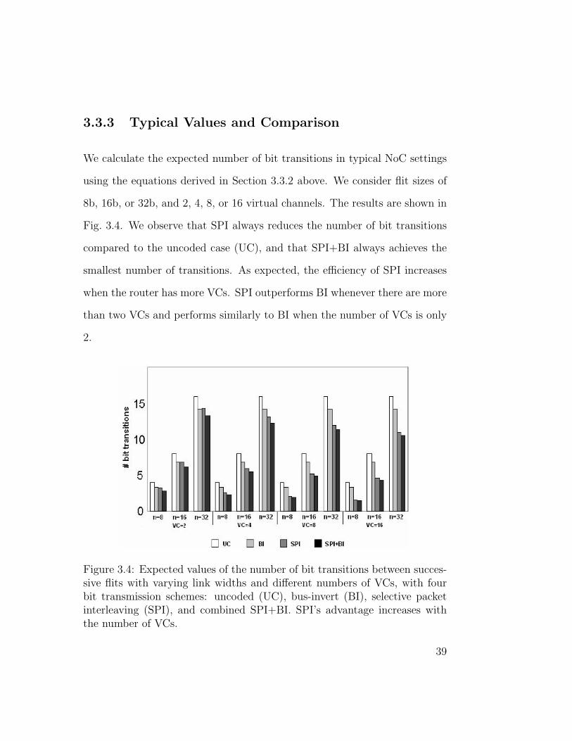
3.3.3 Typical Values and Comparison
We calculate the expected number of bit transitions in typical NoC settings
using the equations derived in Section 3.3.2 above. We consider flit sizes of
8b, 16b, or 32b, and 2, 4, 8, or 16 virtual channels. The results are shown in
Fig. 3.4. We observe that SPI always reduces the number of bit transitions
compared to the uncoded case (UC), and that SPI+BI always achieves the
smallest number of transitions. As expected, the efficiency of SPI increases
when the router has more VCs. SPI outperforms BI whenever there are more
than two VCs and performs similarly to BI when the number of VCs is only
2.
Figure 3.4: Expected values of the number of bit transitions between succes-sive flits with varying link widths and different numbers of VCs, with fourbit transmission schemes: uncoded (UC), bus-invert (BI), selective packetinterleaving (SPI), and combined SPI+BI. SPI’s advantage increases withthe number of VCs.
39
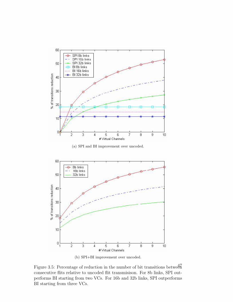
In order to compare SPI and BI, we calculate the reductions they achieve
in the expected number of bit transitions between consecutive flits compared
to uncoded transmissions. We study the cases of 8b, 16b and 32b link widths
for a varying number of VCs. Results are shown in Fig. 3.5(a). We see that
with 8b links, SPI outperforms BI for two or more VCs. In the cases of 16b
and 32b links, SPI outperforms BI with three or more VCs. In all cases, the
gap increases as the number of VCs grows.
We next examine the improvement of SPI+BI over uncoded transmis-
sions. The results are shown in Fig. 3.5(b). We see that as the number
of VCs increases, SPI+BI achieves similar results to those of SPI. That is,
BI’s contribution to the performance of SPI+BI scheme is only significant
when the number of VCs is small. Consider, for example, the case of 8b
wide links: with two VCs, SPI achieves a 20% reduction in the number of
transitions whereas SPI+BI achieves 30%, with eight VCs, SPI’s reduction
is 49% whereas SPI+BI achieves 51%.
We calculate the percentage of improvement of SPI over UC. Fig. 3.6
examines the reduction trend as we vary both the number of VCs and the
link width. We observe that in general, the reduction in the number of
transmissions increases as the ratio #VCs/(link width) increases. For similar
values of #VCs/(link width) and #VCs higher than two, smaller link widths
produce better performance than higher ones.
40
3.4 Benchmark Simulation
In the previous section, we analyzed the bit transmission schemes with ran-
dom traffic. In this section, we simulate the schemes with real workloads of
the file type as used in [31]. We simulate the uncoded, bus-invert, SPI and
the combined SPI+BI flit transmission schemes. In Section 3.4.1 we describe
the simulated model and setup. In Section 3.4.2 we present the benchmark
simulation results, which validate our analysis. In this section, we do not
simulate the VC identification bits. Finally, in Section 3.4.3, we add the
VC identification bits to the transmissions, and examie their impact on the
number of transitions.
3.4.1 Methodology
We use a cycle-accurate router simulator that models the output buffer with
a given number of VCs, a given flit transmission scheme, and the router’s
output link. The model is implemented in MATLAB. We count the number
of bit transitions on the output link with different numbers of VCs, different
benchmark streams, and the four studied flit transmission schemes.
We measure the average number of bit transitions over the link, i.e., the
total number of bit transitions divided by (number of packets)×(flits per
packet) in the streams. We assume that the flit size is equal to the link
width and there are 128 flits per packet. In each simulation, streams of files
of the same benchmark type are transmitted via all VCs of the simulated
41
router, so that all VCs are fully utilized at all time. Each file is sent through
a different VC. Results are shown in Fig. 3.7 with (a) two VCs and 16b width
links; and (b) eight VCs and 8b width links.
The workload file types are the same as used in [31], namely: jpg, pdf,
mp3, bmp, tiff, wav, html, gcc, gzip, raw, and bytecode. For each file type,
we download from the web a random collection of files of this type.
3.4.2 Simulation Results
The simulation results of all benchmarks are depicted in Fig. 3.7. We observe
similar reductions in the number of bit transitions over all benchmarks. With
two VCs and 16b links, the percentage of reduction in bit transitions of SPI
relative to uncoded transmissions ranges from 10% to 13%, whereas with
eight VCs and 8b links, we see reductions of 45%-55%. We also observe that
for one benchmark, raw images, BI increases the number of bit transitions
compared to the uncoded case. This is because of the extra bit (wire) BI
adds on the link. In contrast, SPI and SPI+BI always reduce the number of
bit transitions.
In general, the SPI+BI scheme presents the best results. However, the
gap between SPI+BI and SPI in the tested configuration is small and they
achieve relatively similar results.
We next zoom in on one of the benchmarks, and experiment with it in
a larger design space of parameter values. We simulate the specific MP3
benchmark with the four studied flit transmission schemes and with the VC
42
sizes and link widths used in Section 3.3.3. We do this in order to validate
the analysis results achieved in the previous section. We observe a match be-
tween the analysis as shown in Fig. 3.5 and the MP3 benchmark simulations
presented in Fig. 3.8. This validates our analysis assumptions.
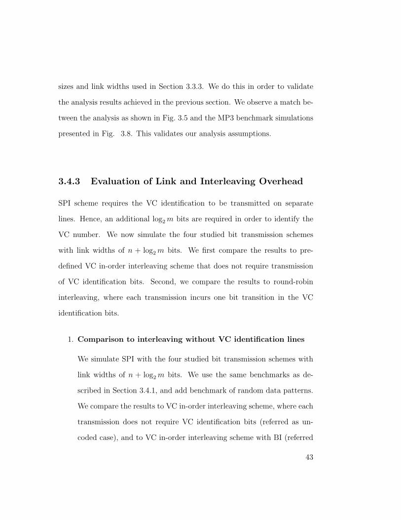
3.4.3 Evaluation of Link and Interleaving Overhead
SPI scheme requires the VC identification to be transmitted on separate
lines. Hence, an additional log2m bits are required in order to identify the
VC number. We now simulate the four studied bit transmission schemes
with link widths of n + log2m bits. We first compare the results to pre-
defined VC in-order interleaving scheme that does not require transmission
of VC identification bits. Second, we compare the results to round-robin
interleaving, where each transmission incurs one bit transition in the VC
identification bits.
1. Comparison to interleaving without VC identification lines
We simulate SPI with the four studied bit transmission schemes with
link widths of n + log2m bits. We use the same benchmarks as de-
scribed in Section 3.4.1, and add benchmark of random data patterns.
We compare the results to VC in-order interleaving scheme, where each
transmission does not require VC identification bits (referred as un-
coded case), and to VC in-order interleaving scheme with BI (referred
43
as BI). In the SPI and SPI+BI schemes, the data bit in the link refer
to n+ log2m bits. Results are shown in Fig. 3.9. We observe 10%-40%
reduction in the number of bit transitions with SPI+VC identification
compared to the in-order interleaving case. SPI+VC identification ad-
vantage increases with the number of VCs.
2. Comparison to adaptive round robin interleaving
We simulate SPI with the four studied bit transmission schemes with
link widths of n+log2m bits. We use the same benchmarks as described
in Section 3.4.1, and add benchmark of random data patterns. We
compare the results to adaptive round-robin interleaving scheme, where
each transmission implies one transitions in the VC identification bits
(referred as uncoded case), and to adaptive round-robin interleaving
with BI (referred as BI). In the SPI and SPI+BI schemes, the data bit
in the link refer to n+ log2m bits. Results are shown in Fig. 3.10. We
observe 15%-55% reduction in the number of bit transitions with SPI
comparing the uncoded case, similarly to the case where the link does
not include VC identification bits. SPI’s advantage increases with the
number of VCs.
3.5 Power Analysis
Having shown that SPI effectively reduces the number of bit transitions, we
proceed to examine the impact this has on power reduction and whether this
44

reduction justifies the overhead of implementing SPI. We have implemented
SPI using verilog HDL, synthesized by Synopsis Design Compiler using the
Tower Semiconductor 0.18µ process library and placed and routed by Ca-
dence Encounter EDA tools. For the NoC link, we assume a wire length of
3mm, and derive its other parameters from the ”global interconnect” set-
ting described by the PTM models in [46]: width of 0.8µ, spacing of 0.8µ,
thickness of 1.25µ, height of 0.65µ and k of 3.5. Input data is assumed to be
random, and all virtual channels are assumed to be fully utilized. We assume
the link width includes flit width and VC identification. SPI is implemented
for two or more virtual channels.
Measurements of the dynamic power dissipated on the link, along with
the power consumed by the SPI module, are jointly referred to as power
consumption. The percentage of reduction in power consumption relative to
uncoded flit transmission is shown in Fig. 3.11. As with bit transitions, we
observe increasing reduction in power consumption with the growing number
of VCs. For example, with 8b width links and four VCs, we observe a power
reduction of more than 25%. With 16b width links and four VCs, we observe
15% power reduction, and with 32b width links and four VCs, a power re-
duction of about 10%. These findings are consistent with the reductions in
bit transitions found in the analysis and benchmark simulations described in
Sections 3.3 and 3.4.
Note that the percentage of power reduction is smaller than the reduction
in the number of bit transitions due to the power overhead of implementing
45

SPI. Nevertheless, in all cases, SPI is cost-effective, and saves more power
than it consumes.
46
(a) SPI and BI improvement over uncoded.
(b) SPI+BI improvement over uncoded.
Figure 3.5: Percentage of reduction in the number of bit transitions betweenconsecutive flits relative to uncoded flit transmisison. For 8b links, SPI out-performs BI starting from two VCs. For 16b and 32b links, SPI outperformsBI starting from three VCs.
47
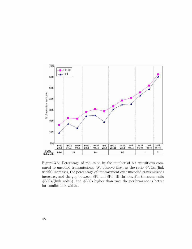
Figure 3.6: Percentage of reduction in the number of bit transitions com-pared to uncoded transmissions. We observe that, as the ratio #VCs/(linkwidth) increases, the percentage of improvement over uncoded transmissionsincreases, and the gap between SPI and SPI+BI shrinks. For the same ratio#VCs/(link width), and #VCs higher than two, the performance is betterfor smaller link widths.
48
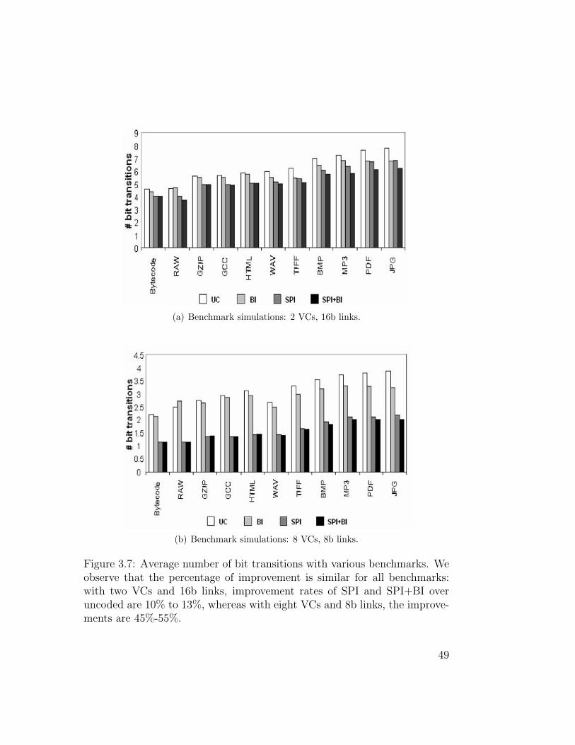
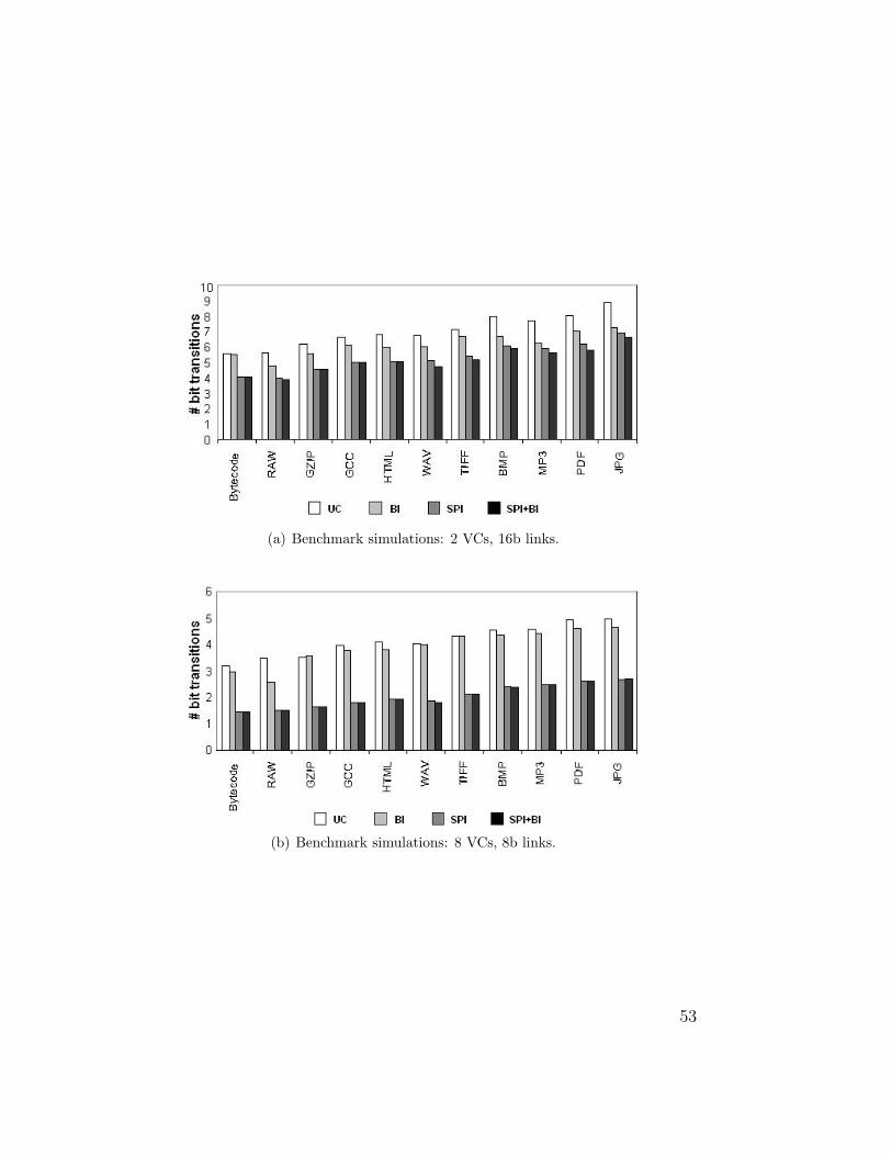
(a) Benchmark simulations: 2 VCs, 16b links.
(b) Benchmark simulations: 8 VCs, 8b links.
Figure 3.7: Average number of bit transitions with various benchmarks. Weobserve that the percentage of improvement is similar for all benchmarks:with two VCs and 16b links, improvement rates of SPI and SPI+BI overuncoded are 10% to 13%, whereas with eight VCs and 8b links, the improve-ments are 45%-55%.
49
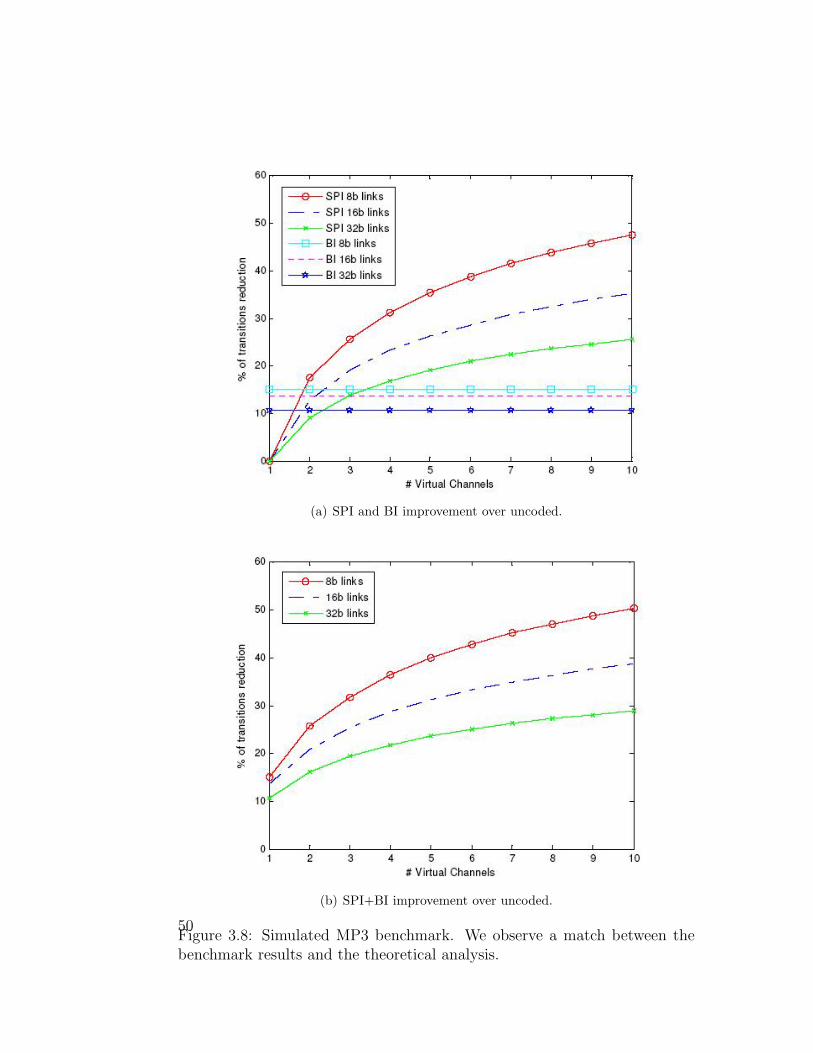
(a) SPI and BI improvement over uncoded.
(b) SPI+BI improvement over uncoded.
Figure 3.8: Simulated MP3 benchmark. We observe a match between thebenchmark results and the theoretical analysis.
50
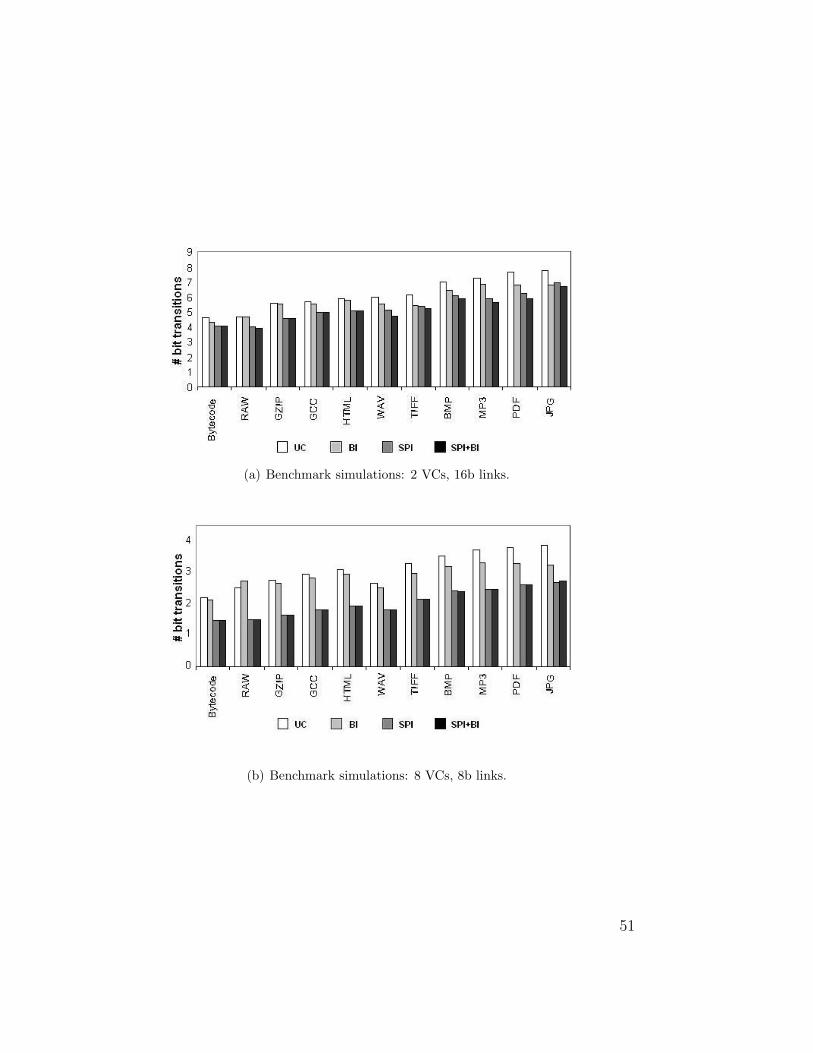
(a) Benchmark simulations: 2 VCs, 16b links.
(b) Benchmark simulations: 8 VCs, 8b links.
51
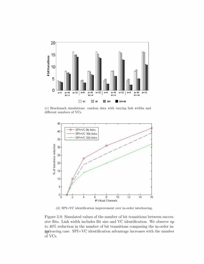
(c) Benchmark simulations: random data with varying link widths anddifferent numbers of VCs.
(d) SPI+VC identification improvement over in-order interleaving.
Figure 3.9: Simulated values of the number of bit transitions between succes-sive flits. Link width includes flit size and VC identification. We observe upto 40% reduction in the number of bit transitions comparing the in-order in-terleaving case. SPI+VC identification advantage increases with the numberof VCs.52
(a) Benchmark simulations: 2 VCs, 16b links.
(b) Benchmark simulations: 8 VCs, 8b links.
53
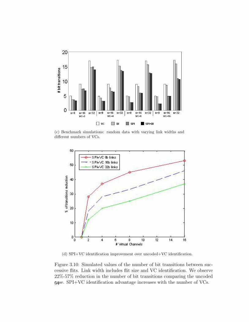
(c) Benchmark simulations: random data with varying link widths anddifferent numbers of VCs.
(d) SPI+VC identification improvement over uncoded+VC identification.
Figure 3.10: Simulated values of the number of bit transitions between suc-cessive flits. Link width includes flit size and VC identification. We observe22%-57% reduction in the number of bit transitions comparing the uncodedcase. SPI+VC identification advantage increases with the number of VCs.54
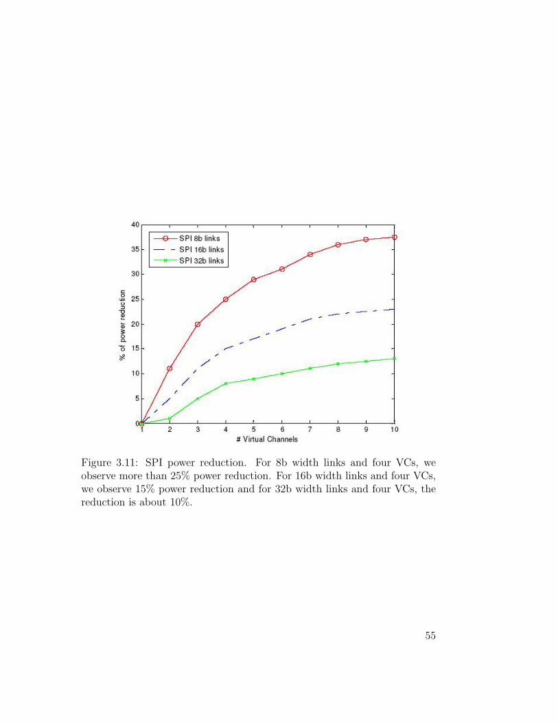
Figure 3.11: SPI power reduction. For 8b width links and four VCs, weobserve more than 25% power reduction. For 16b width links and four VCs,we observe 15% power reduction and for 32b width links and four VCs, thereduction is about 10%.
55

56

Chapter 4
Conclusions
Modern integrated circuits introduce low power design challenges. The lion’s
share of power consumption lies with the interconnect switching activity, and
this share is expected to grow in years to come [1, 12, 33, 34, 38, 44]. In this
thesis we presented two algorithms for power reduction on NoC links.
First, we presented PaR parity routing, a low-overhead error detection
solution for networks on chip. PaR can be used to provide any predefined
error protection requirement. It exploits NoC path diversity, and selects
routing paths based on parity bits. It thus saves the actual transmissions
of these bits, along with the associated power penalty. PaR uses simple,
low-complexity encoding and decoding circuits. We analyzed the savings
achieved by PaR, and showed that it yields significant savings even on small
NoCs, (for example, saving 75% of redundant bit transmissions on a 4x4
NoC mesh), and its savings asymptotically converge to 100% with the size of
57

the NoC. We further showed that PaR can yield power savings (for example,
saving 35% of redundant power consumption on a 3x3 NoC mesh NoC).
Second, we presented SPI - selective packet interleaving, a flit transmis-
sion scheme for energy efficient NoCs. SPI exploits the multiplicity of virtual
channels to transmit a dynamically chosen flit so as to minimize bit tran-
sitions between consecutive flits. SPI uses simple, low-complexity circuits.
We analyzed the savings achieved by SPI, and showed that SPI yields a
significant improvement in power consumption, which outweighs the cost of
implementing SPI. For example, with 8b width links and 4 VCs, SPI reduces
the average number of bit transitions over the link by more than 35%, and
reduces the power consumption by 25%. Analysis and simulations demon-
strate a reduction of up to 55% in the number of bit transitions and up to
40% savings in power consumed on the link. Furthermore, SPI’s benefits
grow with the number of virtual channels.
58

Appendices
59


Lemma .0.1 (Edge Disjoint Routing). For each pair of nodes S and D such
that Sx 6= Dx and Sy 6= Dy, and for every D′ such that Sx 6= D′x and Sy 6= D′y,
the XY (respectively YX) path from S to D′ does not share any edge with the
YX (respectively XY) path from S to D.
Proof. The YX path from S to D traverses vertical edges on coordinates Sx
only, and since Sx 6= Dx, it traverses only horizontal edges that are not on
Sy. On the other hand, the XY path from S to D′ traverses only vertical
edges that are not on Sx and on horizontal edges on Sy only. Thus, these
paths are disjoint. In a similar way, the XY path from S to D is edge-disjoint
to the YX path from S to D′.
Lemma .0.2 (PaR Shortest Path and Complete Routing). PaR Implements
shortest path and complete routing.
Proof. Assume that no error occurs during packet routing. According to PaR
encode functions, the default routing is XY route to D. In case S and D do
not share coordinate and parity bit values are not all zero, then the routing
is either XY or YX toward diagonal node of D. Either case, XY or YX, the
next node is known and the packet advances one hop towards D, therefore
PaR implements shortest path and complete routing.
Lemma .0.3 (PaR Correctness). PaR detects every error according to the
utilized error detection code in transmitted packets. There is no false detec-
tion.
Proof. We distinguish between two cases:
61

1. Sx = Dx or Sy = Dy.
In this case, the source node and destination node share at least one
coordinate. According to the PaR algorithm, in this case, the parity
bits are sent along with the data. The destination node receives the
packet with the parity bits, and therefore it can detect any error.
2. Sx 6= Dx or Sy 6= Dy. There are two kinds of possible errors:
(a) Payload Error: According to Lemma 1, the XY and YX routing
paths between the last node and the target node are edge-disjoint,
and therefore, if there is any change in the bits on any intermediate
edge, the calculated parity bits detects that the incoming edge is
not supposed to be in the routing path.
(b) Change of destination or source nodes in the packet: If
PaR uses one parity bit, then the error will be detected according
to Lemma 1. If PaR uses more than one parity bit, e.g., PaR-
2, according to the PaR-r algorithm, in this case, the source and
destination parity bits of the source and destination nodes are sent
along with the data. The destination node receives the packet with
the parity bits, and therefore it can detect any error.
62

PaR Hardware Architecture
PaR encoder hardware scheme is shown at Fig. 1. Inputs are data,
current hop, source and destination. The parity of the data is calculated
using parity calculation block. According to the parity value (ParVal) the
ParVal decoder block output the routing direction selection to the output
mux. The ParVal decoder block also adds the parity bits to the packet
according to the location of the packet.
Figure 1: PaR encoder hardware architecture.
63
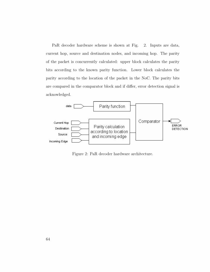
PaR decoder hardware scheme is shown at Fig. 2. Inputs are data,
current hop, source and destination nodes, and incoming hop. The parity
of the packet is concurrently calculated: upper block calculates the parity
bits according to the known parity function. Lower block calculates the
parity according to the location of the packet in the NoC. The parity bits
are compared in the comparator block and if differ, error detection signal is
acknowledged.
Figure 2: PaR decoder hardware architecture.
64
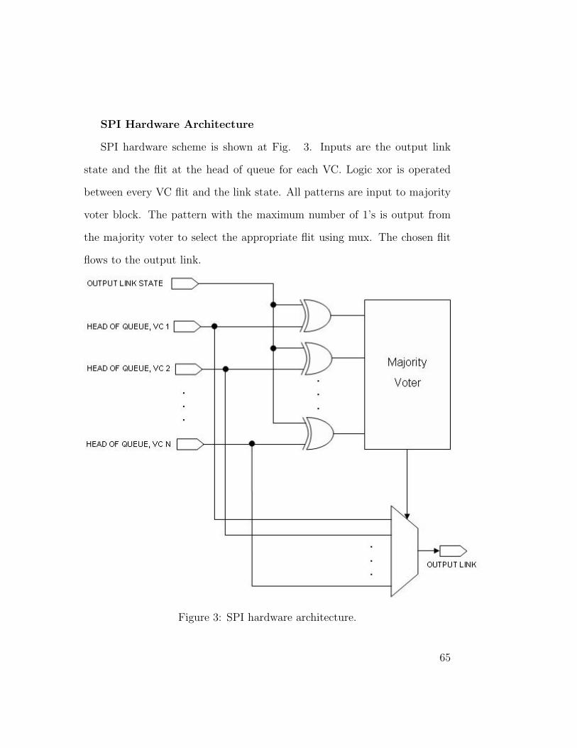
SPI Hardware Architecture
SPI hardware scheme is shown at Fig. 3. Inputs are the output link
state and the flit at the head of queue for each VC. Logic xor is operated
between every VC flit and the link state. All patterns are input to majority
voter block. The pattern with the maximum number of 1’s is output from
the majority voter to select the appropriate flit using mux. The chosen flit
flows to the output link.
Figure 3: SPI hardware architecture.
65

66
Bibliography
1. A. Banerjee, R. Mullins, S. Moore, ”A Power and Energy Exploration of
Network-on-Chip Architectures”, International Symposium on Networks-
on-Chip (NOCS), pp. 163-172, 2007.
2. A. Berman, I. Keidar, ”Low Overhead Error Detection for Networks-
on-Chip”, International Conference on Computer Design (ICCD), pp.
219-225, 2009.
3. A. Berman, R. Ginosar, I. Keidar, ”Order is Power: Selective Packet In-
terleaving for Energy Efficient Networks-on-Chip”, submitted for pub-
lication.
4. L. Benini, A. Macii, E. Macii, M. Poncino, R. Scarsi. ”Architecture
and Synthesis Algorithms for Power-Efficient Bus Interfaces”, IEEE
Transactions on Computer-Aided Design of Integrated Circuits and
Systems (ICCAD), Vol. 19, pp. 969-980, Sept. 2000.
5. L. Benini, G. De Micheli, ”Powering Networks on Chips”, 14th inter-
67

national symposium on Systems synthesis (ISSS) pp.33-38, Oct. 2001.
6. V. Chandra, A. Xu, H. Schmit, ”A Low Power Approach to Sys-
tem Level Pipelined Interconnect Design”, International Workshop on
System-Level Interconnect Prediction (SLIP), Feb. 2004.
7. W.J. Dally and B. Towles, ”Route Packets, Not Wires: On-Chip Inter-
connection Networks, Proceedings of Design Automation Conference
(DAC), pp. 684-689, 2001.
8. S. Devadas and S. Malik, ”A Survey of Optimization Techniques Tar-
geting Low Power VLSI Circuits”, Proceedings of the 32nd annual
ACM/IEEE Design Automation Conference (DAC), pp. 242-247, 1995.
9. R. Dobkin, A. Morgenshtein, A. Kolodny, R. Ginosar, ”Parallel vs.
Serial On-Chip Communication”, International Workshop on System-
Level Interconnect Prediction (SLIP), April. 2008.
10. A. Dutta and N. A. Touba, ”Reliable Network-on-Chip Using a Low
Cost Unequal Error Protection Code”, 22nd IEEE International Sym-
posium on Defect and Fault Tolerance in VLSI Systems, 2007, pp. 3-11.
11. R. Golshan, B. Haroun, ”A novel reduced swing CMOS BUS interface
circuit for high speed low power VLSI systems”, IEEE International
symposium on circuits and systems (ISCAS), pp. 351-354, Jun. 1994.
12. P. Grosse1, Y. Durand and P. Feautrier, ”Power Modeling of a NoC
68
Based Design for High Speed Telecommunication Systems”, Proceed-
ings of the 16th international workshop on Integrated Circuit and Sys-
tem Design. Power and Timing Modeling, Optimization and Simula-
tion (PATMOS) Sept. 2006.
13. P. Guerrier , A. Greiner,A generic architecture for on-chip packet-
switched interconnections, Design, Automation and Test in Europe
Conference and Exhibition 2000. pp. 250 256.
14. A. Hemani, A. Jantsch, S. Kumar, A. Postula, J. Oberg, M. Millberg,
D. Lindqvist, Network on a Chip: An architecture for billion transistor
era, In Proceeding of the IEEE NorChip Conference, Nov. 2000.
15. J. Hu, R. Marculescu, ”Exploiting the Routing Flexibility for En-
ergy/Performance Aware Mapping of Regular NoC Architectures”, Pro-
ceedings of Design, Automation and Test in Europe Conference and
Exhibition (DATE), Feb. 2004.
16. C. Jose et-al. , ”Adaptive Coding in Networks-on-Chip: Transition
Activity Reduction Versus Power Overhead of the Codec Circuitry,
Proceedings of the 16th international workshop on Integrated Circuit
and System Design. Power and Timing Modeling, Optimization and
Simulation (PATMOS) Sept. 2006.
17. W. Kim, J. Kim, S. Min, ”A Dynamic Voltage Scaling Algorithm for
Dynamic-Priority Hard Real-Time Systems Using Slack Time Analy-
69
sis”, Design, Automation and Test in Europe Conference and Exhibi-
tion (DATE) 2002.
18. R. Krishnan, J. Gyvez, H. Veendrick, ”Encoded-Low Swing Technique
for Ultra Low Power Interconnect”, Field Programmable Logic and
Applications, pp. 240-251, Spring Publishers, 2003.
19. S. Kumar, A. Jantsch, J.P. Soininen, M. Forsell, M. Millberg, J. Berg,
K. Tiensy and A. Hemani, ”A Network on Chip Architecture and De-
sign Methodology”,” IEEE Computer Society Annual Symposium on
VLSI (ISVLSI), pp. 105-112, Apr. 2002.
20. K. Lee, S.J. Lee and H.J. Yoo, ”Low-Power Network-on-Chip for High-
Performance SoC Design”, IEEE Transactions on Very Large Scale
Integration (VLSI) Systems, Vol. 14, pp. 148-160, Feb. 2006.
21. E. Macii, ”Ultra low power electronics and design”, Kluwer Academic
Publishers, Chp. 12, pp. 214-233, 2004.
22. N. Magen, A. Kolodny, U. Weiser and N. Shamir, ”Interconnect-Power
Dissipation in a Microprocessor”, Proceedings of the 6th International
Workshop on System-Level Interconnect Prediction (SLIP), Feb. 2004.
23. C. Marcon1, N. Calazans, F. Moraes, A. Susin, I. Reis and F. Hessel,
”Exploring NoC Mapping Strategies: An Energy and Timing Aware
Technique”, Proceedings of Design, Automation and Test in Europe
Conference (DATE), pp. 502-507, 2005.
70

24. H. Mehta, R. Owens, M. J. Irwin. ”Some Issues in Gray Code Address-
ing”, GLS-VLSI-96, pp. 178-180, Mar. 1996.
25. G. Micheli, L. Benini, ”Networks on Chips Technology and Tools”,
Morgan Kaufmann Publishers 2006, pp. 75-139.
26. F. Moraes, N. Calazans, A. Mello, L. M?ller and L. Ost, ”HERMES:
an infrastructure for low area overhead packet-switching networks on
chip”, Integration, the VLSI Journal, Vol. 38, pp. 69-93, Oct. 2004.
27. A. Morgenshtein, E. Bolotim, I. Cidon, A. Kolodny, R. Ginosar, ”Micro
Modem Reliability Solution For NoC Communications”, ICECS 2004,
pp. 483-486.
28. S. Murali, T. Theocharides, N. Vijaykrishnan, M.J Irwin, L. Benini, G.
Micheli, ”Analysis of Error Recovery Schemes for Networks on Chips”,
IEEE Design&Test of Computers 2005, pp. 434-442.
29. M. Mutyam, ”Selective shielding: A Crosstalk-Free Bus Encoding Tech-
nique”, IEEE ICCAD 2007, pp.618-621.
30. J. Nurmi, H. Tenhunen, J. Isoaho, A. Jantsch, ”Interconnect-Centric
Design for Advanced SOC and NOC”, Kluwer Academic Publishers
2004, pp. 155-170.
31. J. Palma, L. Indrusiak, F.G. Moraes, A. Garcia Ortiz, M. Glesner, R.
Reis, ”Inserting Data Encoding Techniques into NoC-Based Systems”
71

IEEE Computer Society Annual Symposium on VLSI (ISVLSI), pp.
299-304, March 2007.
32. D. Park, C. Nicopoulos, J. Kim, N. Vijaykrishnan, C.R. Das, ”Explor-
ing Fault-Tolerant NoC Architectures”, IEEE DSN 2006, pp. 93-104.
33. V. Raghunathan, M.B. Srivastava and R.K. Gupta, ”A survey of tech-
niques for energy efficient on-chip communication”, Proceedings of De-
sign Automation Conference (DAC), pp. 900-905, 2003.
34. P. Ramos, A. Oliveira, ”Low Overhead Encodings For Reduced Activ-
ity in Data And Address Buses”, IEEE International Symposium on
Signals, Circuits and Systems, 1999.
35. S. Ramprasad, N.R. Shanbhag and I.N. Hajj,, ”A Coding Framework
for Low-Power Address and Data Busses”, IEEE Transactions on Very
Large Scale Integration (VLSI) Systems, Vol. 7, pp. 212-221, Jun.
1999.
36. E. Salminen, A. Kulmala and T.D. Hamalainen, ”Survey of Network-
on-chip proposals”, white paper, OCP-IP, March 2008.
37. M. Stan and W. Burleson, ”Bus-Invert Coding for Low-Power I/O”,
IEEE Transactions on Very Large Scale Integration (VLSI) Systems,
Vol. 3, pp. 49-58, 1995.
38. K. Sundaresan and N.R. Mahapatra, ”Accurate Energy Dissipation
and Thermal Modeling for Nanometer-Scale Buses”, Proceedings of
72
the 11th Int’l Symposium on High-Performance Computer Architecture
(HPCA) 2005.
39. B. Towles and W.J. Dally, ”Worst-case Traffic for Oblivious Routing
Functions”, Computer Architecture Letters, February 2002.
40. A. Vitkovski, R. Haukilahti, A. Jantsch, E. Nilsson, ”Low Power and
Error Coding for Network-on-Chip Traffic”, Norchip Conference Proc.,
2004, pp. 20-23.
41. P. Vellanki, N. Banerjee, K.S. Chatha, ”Quality-of-Service and Error
Control Techniques for Mesh-Based Network-on-Chip Architectures”,
Integration 2005, pp. 353-382.
42. H. Wang, L.S. Peh, S. Malik, ”Power-driven Design of Router Microar-
chitectures in On-chip Networks”, 36th Annual IEEE/ACM Interna-
tional Symposium on Microarchitecture (MICRO), Dec. 2003.
43. H. Zhang, V. George, J. Rabaey, ”Low-Swing On-Chip Signaling Tech-
niques: Effectiveness and Robustness”, IEEE Transactions on very
large scale integration (VLSI) systems, Vol. 8, No. 3, June 2000.
44. L. Zhong, N.K. Jha, ”Interconnect-aware High-level Synthesis for Low
Power”, International Conference on Computer Aided Design (ICCAD),
2002.
45. H. Zimmer, A. Jantsch, ”Fault Model Notation and Error Control
73

Scheme for Switch to Switch buses on NoC”, CODES ISSS 2003, pp.
188-193.
46. Arizona State University, Predictive Technology Model [Online]. Avail-
able at http://www.eas.asu.edu/ ptm/
74