PoWR grids of non-LTE model atmospheres for OB-type stars ...ftp/wrhamann/hainich-ob-grid-2019.pdf2 Institute of astrophysics, KU Leuven, Celestijnlaan 200D, 3001 Leuven, Belgium 3

Astronomy & Astrophysics manuscript no. paper c©ESO 2018November 16, 2018

PoWR grids of non-LTE model atmospheres for OB-type stars ofvarious metallicities

R. Hainich1, V. Ramachandran1, T. Shenar1, 2, A. A. C. Sander1, 3, H. Todt1, D. Gruner1, L. M. Oskinova1, and W.-R.Hamann1

1 Institut für Physik und Astronomie, Universität Potsdam, Karl-Liebknecht-Str. 24/25, D-14476 Potsdam, Germanye-mail: [email protected]

2 Institute of astrophysics, KU Leuven, Celestijnlaan 200D, 3001 Leuven, Belgium3 Armagh Observatory and Planetarium, College Hill, Armagh, BT61 9DG, Northern Ireland

Received <date> / Accepted <date>

ABSTRACT

The study of massive stars in different metallicity environments is a central topic of current stellar research. The spectral analysisof massive stars requires adequate model atmospheres. The computation of such models is difficult and time-consuming. Therefore,spectral analyses are greatly facilitated if they can refer to existing grids of models. Here we provide grids of model atmospheresfor OB-type stars at metallicities corresponding to the Small and Large Magellanic Clouds, as well as to solar metallicity. In total,the grids comprise 785 individual models. The models were calculated using the state-of-the-art Potsdam Wolf-Rayet (PoWR) modelatmosphere code. The parameter domain of the grids was set up using stellar evolution tracks. For all these models, we providenormalized and flux-calibrated spectra, spectral energy distributions, feedback parameters such as ionizing photons, Zanstra temper-atures, and photometric magnitudes. The atmospheric structures (the density and temperature stratification) are available as well. Allthese data are publicly accessible through the PoWR website.

Key words. Stars: massive – Stars: early type – Stars: atmospheres – Stars: winds, outflows – Stars: mass-loss – Radiative transfer

1. Introduction

Through their powerful stellar winds, ionizing fluxes, and su-pernova (SN) explosions, massive stars (Mi & 8 M�) dominatethe energy budget of their host galaxies. They are the progeni-tors of core-collapse SNe, leaving behind a neutron star (NS) ora black hole (BH), which makes them central players in mod-ern gravitational-wave (GW) astrophysics (e.g., Marchant et al.2016; de Mink & Mandel 2016; Hainich et al. 2018). Spectro-scopically, they are predominantly identified with O and earlyB spectral types. When surrounded by thick stellar winds, theyare classified as Wolf-Rayet (WR) stars (Smith 1968; Smithet al. 1996), as transition-type stars, such as Of/WN stars (e.g.,Crowther & Walborn 2011), or as luminous blue variables(LBVs; e.g., Humphreys & Davidson 1994; van Genderen 2001)

In recent years, the topic of massive stars at low metallic-ity (Z) has been gaining tremendous momentum. The first starsthat formed in our universe must have been born in extremelyZ-poor environments (Bromm & Larson 2004). Massive bina-ries at low Z are the leading candidates for massive GW mergersystems (e.g., Eldridge & Stanway 2016). Generally, massivestars as a function of Z are intensively studied; for example,the Z−dependence of multiplicity parameters (Sana et al. 2013;Almeida et al. 2017), initial masses (Schneider et al. 2018), bi-nary interaction physics (Foellmi et al. 2003; Shenar et al. 2016,2017), stellar feedback (Ramachandran et al. 2018a,b), stellarrotation (Meynet & Maeder 2005), and stellar winds (Mokiemet al. 2007; Hainich et al. 2015). The Small and Large Mag-ellanic Clouds (SMC, LMC), with their well-constrained dis-tances, low interstellar extinctions, and subsolar metallicity of∼1/7 and 1/2 solar, respectively (Dufour et al. 1982; Larsen et al.

2000; Trundle et al. 2007), offer ideal laboratories for studyingZ-dependent effects.

The physical parameters of massive stars, such as their tem-peratures, luminosities, and masses, can be derived by com-paring observed to synthetic spectra. To model massive staratmospheres, it is essential to allow for non-local thermody-namic equilibrium (non-LTE), and to account for the millionsof iron-line transitions in the ultraviolet (UV) that give riseto the so-called line-blanketing (e.g., Hubeny & Lanz 1995;Hillier & Miller 1998). For most O-type stars, as well as forevolved B-type stars, a calculation of the wind is also required(Hamann 1981; Kudritzki et al. 1992; Puls et al. 2008). There areonly a few codes worldwide that fulfill these requirements (seeoverviews in, e.g., Puls 2008; Sander et al. 2015).

The Potsdam Wolf-Rayet (PoWR) model atmosphere pro-gram is one of these codes. Originally developed for WR stars,it is now applicable to any hot star that does not show significantdeviations from spherical symmetry, including OB-type stars(Gräfener et al. 2002; Hamann & Gräfener 2003; Sander et al.2015). Using PoWR, fundamental parameters have been derivedfor many WR stars and binaries in the Galaxy (Hamann et al.1995; Sander et al. 2012) and the Magellanic Clouds (Hainichet al. 2014; Shenar et al. 2016), as well as for OB-type starsand binaries (Shenar et al. 2015; Ramachandran et al. 2018a).PoWR model grids for WR stars of various types and at vari-ous metallicites have been published online1 (Sander et al. 2012;Hamann & Gräfener 2004; Todt et al. 2015). With the currentpaper, we announce the publication of extensive model grids ofOB-type stars at SMC, LMC, and solar metallicities calculated

1 www.astro.physik.uni-potsdam.de/PoWR

Article number, page 1 of 12

arX

iv:1

811.

0630

7v1

[as

tro-

ph.S

R]

15

Nov

201

8

www.astro.physik.uni-potsdam.de/PoWR

A&A proofs: manuscript no. paper

SMCLMCMW

2.0

2.5

3.0

3.5

4.0

4.5

15 20 25 30 35 40 45 50 55

T*

[kK]

log

gg

rav [

cg

s]

Fig. 1. Overview of OB-type model grids in the T∗ − log ggrav plane. Each symbol represents an available PoWR model. The different colors andsymbols indicate the different grids described in Sect. 3. The extension of the two SMC grids is identical.

with the PoWR code. The applicability of these model gridsranges from spectral analyses of OB-type stars to theoretical ap-plications that need model spectra as an input such as populationsynthesis (e.g., Leitherer et al. 2014; Eldridge et al. 2017), orapplications that require atomic level population numbers as in-put such as three-dimensional (3D) Monte-Carlo calculations ofstellar winds (e.g.. Šurlan et al. 2012a,b).

The paper is structured as follows. In Sect. 2 we describe thebasics of the PoWR atmosphere models. The OB-type grids, thedata products, and the web interface are introduced in Sect. 3.In Sect. 4 we discuss some findings based on our model calcula-tions. Finally, we give a short overview of potential applicationsin Sect. 5.

2. The models

The synthetic spectra presented in this work are calculated withthe Potsdam Wolf-Rayet (PoWR) code, which is a state-of-the-art code for expanding stellar atmospheres. PoWR assumesspherical symmetry and a stationary outflow. It accounts for non-LTE effects, a consistent stratification in the hydrostatic (lower)part of the atmosphere, iron line blanketing, and wind inhomo-geneities. The code solves the rate equations for the statisticalequilibrium simultaneously with the radiative transfer, which iscalculated in the comoving frame. At the same time, the codeensures energy conservation. For details on the code, we refer toGräfener et al. (2002), Hamann & Gräfener (2003), Todt et al.(2015), and Sander et al. (2015).

The main parameters of OB-type models are the stellar tem-perature T∗, the luminosity L, the surface gravity log ggrav, themass-loss rate M, and the terminal wind velocity v∞. The stellartemperature and the luminosity specify the stellar radius R∗ via

the Stefan-Boltzmann law

L = 4πσSBR2∗T

4∗ . (1)

The stellar radius is by definition the inner boundary of themodel atmosphere, which we locate at a Rosseland continuumoptical depth of τRoss = 20. The stellar temperature T∗ is then theeffective temperature that corresponds to R∗. The outer boundaryis set to Rmax = 100 R∗.

In the subsonic part of the stellar atmosphere, the veloc-ity field v(r) is calculated self-consistently such that a quasi-hydrostatic density stratification is obtained. A classical β-law(Castor & Lamers 1979; Pauldrach et al. 1986)

v(r) = v∞(1 − R0

r

)β, (2)

with R0 ≈ R∗ is assumed in the wind, which corresponds to thesupersonic part of the atmosphere. For the exponent, the valueβ = 0.8 is assumed for all models (Kudritzki et al. 1989; Pulset al. 1996).

In the comoving-frame calculations, turbulent motion is ac-counted for by using Gaussian line profiles with a Doppler widthof 30 km/s. This choice is motivated by the requirement to limitthe computation time; tests revealed that narrower line profilesduring the comoving-frame calculations have very limited im-pact on the resulting stratification. In the hydrostatic equation,the turbulent pressure is taken into account by means of a micro-turbulent velocity ξ (see Sander et al. 2015).

After an atmosphere model is converged, the synthetic spec-trum, also denoted as emergent spectrum, is calculated by inte-grating the source function in the observers frame along emerg-ing rays parallel to the line-of-sight. In this formal integral the


R. Hainich et al.: PoWR grids of non-LTE model atmospheres for OB-type stars of various metallicities

T*

/kK

510204060

ZAMS

7 M

9 M

12 M

15 M

25 M

40 M

60 M

3.0

3.5

4.0

4.5

5.0

5.5

6.0

4.5 4.0 3.5

log (T*

/K)

log

(L

/L)

Fig. 2. Hertzsprung-Russell diagram illustrating the coverage of thelog T∗-log L domain by our SMC model-grid. Each blue triangle refersto one grid model. The depicted stellar evolution tracks were calculatedby Brott et al. (2011).

Doppler velocity is decomposed into a depth-dependent ther-mal component and the microturbulent velocity, which is set toξ(R∗) = 14 km/s at the base of the wind and grows proportionalto the wind velocity up to a value of ξ(Rmax) = 0.1 v∞.

Wind inhomogeneities are accounted for by assuming opti-cally thin clumping. The clumping factor D (which is the inverseof the volume filling factor, fV = D−1) describes the over-densityin the clumps compared to a homogeneous model with the samemass-loss rate (Hillier 1991; Hamann & Koesterke 1998), whilethe interclump medium is considered to be void. We assume thatclumping starts at the sonic point and reaches its maximum valueD = 10 at a stellar radius of 10 R∗ (cf. Runacres & Owocki2002).

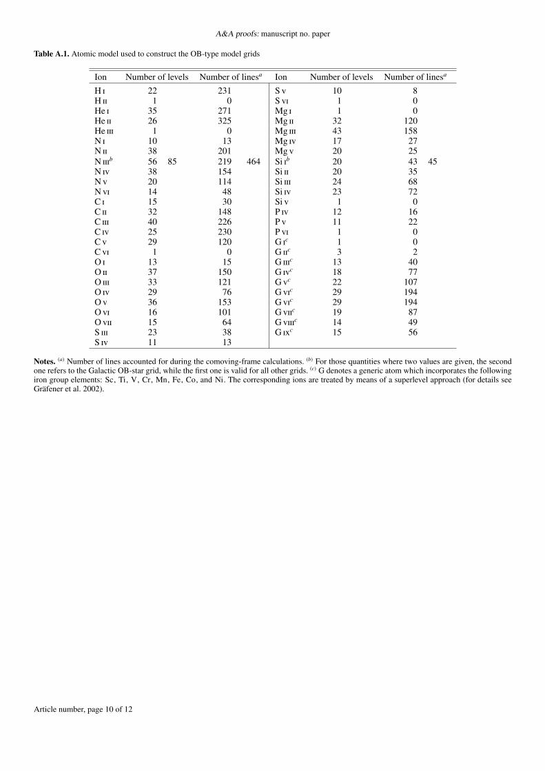
Detailed model atoms of H, He, C, N, O, Mg, Si, P, and Swere included in the non-LTE calculations (see Table A.1). Theiron group elements (Sc, Ti, V, Cr, Mn, Fe, Co, and Ni) withtheir multitude of levels and line transitions were treated in asuperlevel approach (see Gräfener et al. 2002), combining lev-els and transitions into superlevels with pre-calculated transitioncross-sections and with the assumption of solar abundance ratiosrelative to iron.

3. The OB-type atmosphere grids

The PoWR code is employed to construct grids of model at-mospheres for early B-type and O-type stars. Altogether fourgrids have been calculated so far, ranging from solar metallic-ities down to LMC (ZLMC ≈ 1/2 Z�) and SMC metallicities(ZSMC ≈ 1/7 Z�, Dufour et al. 1982; Larsen et al. 2000; Trundleet al. 2007). Two grids have been established for the SMC, whichcorrespond to two different mass-loss rates, while only one gridhas been calculated for the LMC and one for the Galaxy. Theparameterization of the grids is illustrated in Fig. 1. In total 785models have been calculated. Further grids that will improve the

coverage of the mass-loss domain are currently in preparationand will be made available in the near future.

The independent parameters of the grid models are the stellartemperature T∗ and the surface gravity. The grid spacing is 1 kKfor T∗ and 0.2 dex for log ggrav. The gravitational acceleration isgiven by

ggrav =GMR2∗

, (3)

where M is the stellar mass and G the gravitational constant. Forthe SMC and LMC grids, models have been calculated for stel-lar temperatures of 15 kK to 50 kK, while the temperature rangeis 15 − 56 kK for the Galactic grid. Besides T∗ and log ggrav, theluminosity is a further model parameter. The value of L has beenset by using stellar evolution tracks and by interpolating amongthem. Because of that, the extension of the grids in the log ggravdomain is limited by the coverage of the stellar evolution tracks.This is illustrated in Fig. 2 that depicts a Hertzsprung-Russelldiagram (HRD) with the SMC model grid and the stellar evo-lution models used to construct this grid. The correspondingplots for the other grids can be found in Appendix B. For theSMC and LMC grids, the stellar evolution models calculated byBrott et al. (2011) were employed, while the models by Ekströmet al. (2012) were used for the Galactic grid, since those evolu-tion models have a superior coverage of the initial mass domain.These different sets of evolution models are the reason why theextension of the grids is not the same for the MW, LMC, and thetwo SMC grids as visible in Fig. 1.

Based on T∗, L, and log ggrav, the escape velocity for eachmodel is calculated, which in turn is used to estimate the termi-nal wind velocity by applying the scaling relations established byLamers et al. (1995). Accounting for the hot bi-stability jump, afactor of 1.3 is used for stars with T∗ < 21 kK, while 2.6 is ap-plied above 21 kK (see also Lamers & Cassinelli 1999). In addi-tion, the terminal wind velocities for the SMC and LMC modelsare scaled with (Z/Z�)0.13, following Leitherer et al. (1992).

A further model parameter is the mass-loss rate M or, equiv-alently, the wind strength parameter log Q, which is used insteadof M in the two SMC grids to prescribe the wind mass-loss. Inthe PoWR code, the following definition of the log Q parameteris adopted

Q =M/(M�/yr) · D1/2

(v∞/(km/s) · R∗/R�)3/2 , (4)

(see e.g., Puls et al. 1996, 2008; Sander et al. 2017). The twoSMC grids are calculated with log Q = −13.0 and log Q =−12.0, respectively. The use of a fixed log Q in those grids im-plies that the mass-loss rate is not constant throughout the grids,since v∞ and R∗ vary from model to model. In the MW and LMCgrid, we instead used a fixed mass-loss rate of M = 10−7M�/yrfor all models. This value of M is chosen because our grids aremeant as an extension of the parameter space of earlier grids,such as those published by Lanz & Hubeny (2003, 2007), tosignificant mass-loss rates. Hence, a certain amount of wind isalways present in our models. The models calculated by Lanz& Hubeny (2003, 2007) with their TLUSTY code adopt the ap-proximation of a plane-parallel and static atmosphere. Sanderet al. (2015) showed that in the limit of vanishing M and infinitecurvature radius, the emergent spectra of PoWR model atmo-spheres agree very well with the TLUSTY results.

The mass-loss rate is an import parameter that significantlydetermines the density in the wind and, consequently, also theemergent spectrum. The spectral range that is influenced the



He

II 1

2-4

NII

I

SiIV

Hδ

SiIV

He

I 2p

3 Po-5

s3 S

He

I 2p

1 Po-6

d1 D

OII

CII

He

II 1

1-4

SiIV

0.6

0.8

1.0

1.2

4100 4150 4200

λ / Ao

No

rmali

zed

flu

x

OII

CII

I

NII

I

CIV

CII

I

4630 4640 4650 4660 4670 4680

λ / Ao

Fig. 3. Normalized line spectra of the models with T∗ = 36 kK and log ggrav = 3.8 [cgs] from the grid with SMC (red dotted line), LMC (greendashed line), and solar (black continuous line) metallicity. The mass-loss rate of all models is M = 10−7 M�/yr. Two exemplary wavelength rangeswith prominent metal lines are depicted.

most by the choice of M is the UV with its key diagnostic windlines such as N v λλ1239, 1243 Å, Si iv λλ1393.8, 1402.8 Å,C iv λλ1548, 1550.8 Å, He ii λ1640 Å and N iv λ1718 Å. Due tothe choice of modest mass-loss rates for the presented grids,the emergent spectra of all models show at least some of thoselines in the form of P Cygni profiles, depending on the specificionization structure. In comparison to the UV, the optical wave-length range is significantly less influenced by mass loss. In thisrange, the main wind-contaminated lines are He ii λ4686 Å andHα. While Hα might show a certain amount of wind emissionin its profile for the cool models with low surface gravities, theadopted mass-loss rates are usually too low to push He ii λ4686 Åinto emission. Besides these two prominent lines, weaker nitro-gen and carbon lines might appear in emission, as illustrated inthe right panel of Fig. 3. In the infrared (IR), the most prominentline that is influenced by the wind and consequently by M is Brγ,which shows an emission component preferentially in the O-starmodels.

For the galactic grid, we assume solar abundances as derivedby Asplund et al. (2009). In the LMC and SMC models, we adoptthe abundances obtained by Hunter et al. (2007) and Trundleet al. (2007) for C, N, O, Mg, Si, and Fe. For P and S, we usethe corresponding solar abundances, scaled to the metallicity ofthe LMC and SMC by a factor of 1/2 and 1/7, respectively. Thehydrogen mass fraction is set to XH = 0.74 in all models.

In the comoving-frame calculations of the LMC and MWgrid models, a micro turbulent velocity of ξ = 10 km/s is used,while the SMC models are calculated with ξ = 14 km/s.

3.1. Data products

The most important output of the model calculations are thesynthetic line spectra. We provide a continuous coverage fromthe UV to the near-IR (NIR) (920 Å − 2.4 µm), including theK-band, as well as a significant fraction of the mid-IR do-main (10 to 20 µm). These emergent spectra are calculated in

-20

-15

-10

-5

2.0 2.5 3.0 3.5 4.0 4.5 5.0 5.5 6.0

log λ [Ao

]

log

F λ [

erg

s-1 c

m-2

Ao-1

]

Fig. 4. Spectral energy distributions of the three models shown in Fig. 3in comparison with a black body of the same effective temperature asthe models. The models are plotted with the same line styles and colorsas in Fig. 3, while the black body is depicted by a thick gray dashed line.

the observer’s frame and have a spectral resolution of aboutR = 160.000 (corresponding to 5 km/s in the velocity space).Flux-calibrated and continuum-normalized spectra are available.The normalized line spectra of two exemplary wavelength rangeswith prominent metal lines are displayed in Fig. 3. This figure il-lustrates the spectral differences between late O-type giants atdifferent metallicities by comparing models with the same T∗,log ggrav, and M from the different models grids.

We also provide spectral energy distributions (SEDs) overthe whole spectrum. These SEDs include all lines but are ona coarse wavelength grid and were calculated in the comovingframe. The SEDs for the three models depicted in Fig. 3 are plot-ted in Fig. 4 in comparison to a back body with Teff = 36 kK.

Feedback parameters such as the number of hydrogen ion-izing and helium ionizing photons and Zanstra temperatures areavailable for all models. In addition, we provide Johnson U, B,



Table 1. Feedback parameters and magnitudes of the three models fromFigs. 3, 4, and 5.

MW LMC SMClog QH [s−1] 48.83 48.82 48.82TZanstra,H [kK] 35.5 35.3 35.4log QHe i [s−1] 47.80 47.78 47.81log QHe ii [s−1] -b -b 42.06TZanstra,He [kK] -b -b 27.9MU [mag] −6.60 −6.58 −6.54MB [mag] −5.42 −5.41 −5.37MV [mag] −5.12 −5.11 −5.08Mu [mag]a −5.52 −5.50 −5.46Mb [mag]a −5.23 −5.23 −5.19Mv [mag]a −5.31 −5.31 −5.27My [mag]a −5.14 −5.14 −5.10

Notes. (a) Stroemgren magnitudes (b) For these relatively cool models,the Heii ionizing flux (λ < 228 Å) is neglidgeble.

and V magnitudes and Stroemgren u, v, b, and y magnitudes. InTable 1, the predicted magnitudes and feedback parameters arelisted, exemplary for the models shown in Figs. 3 and 4.

The atmospheric structure (e.g., the density and the veloc-ity stratification) is supplied for all models. As an example,the structure information of the model with T∗ = 25 kK andlog ggrav = 3.2 [cgs] from the LMC model grid is listed in Ta-ble A.2.

3.2. The web interface

All information described in Sect. 3.1 can be accessed via thePoWR web interface2. A general description of the interface andhow to use it can be found in Todt et al. (2015). Recently, anoption to obtain the tabulated atmospheric structure and the pos-sibility to download the selected data product for a whole gridwas added to the online interface. Both these options are avail-able after having selected a specific model from the grids. Moredetailed information such as the population numbers or high-resolution SEDs calculated in the observer’s frame are currentlynot accessible via the web interface, but can be provided on in-dividual request.

4. Discussion

Figure 3 reveals how the metal lines become weaker with de-creasing metallicity. A close inspection of this figure, how-ever, also shows that the equivalent widths of the He ii linesare decreasing with Z. A zoom on the He ii λ4542 line and theHe i λ4713 line is depicted in Fig. 5, revealing that as the He iilines get weaker the He i lines simultaneously become strongerwith decreasing Z. Although this effect is relatively small forthe He ii lines, it can have a noticeable impact on the parametersthat one would deduce from spectral line fits using these models.This effect is not limited to the helium lines. Test calculationsrevealed that it is a general trend that is also displayed by otherelements. For example, if the carbon abundance is kept constantbut the iron abundance is changed from its default values in thegrids to zero, the same effect is also visible in the carbon lines.We are confident that this is not a PoWR specific artefact, since

2 www.astro.physik.uni-potsdam.de/PoWR

He

I 2p

3 Po-4

s3 S

0.8

1.0

1.2

4712 4714 4716

λ / Ao

No

rmali

zed

flu

x NII

I

He

II 9

-4

4540 4550

λ / Ao

Fig. 5. As in Fig. 3 but showing zooms on the He I λ4713 andHe II λ4542 line.

the same effect is also shown by the TLUSTY models calculatedby Lanz & Hubeny (2003).

The reason for the observed dependence of the He i to He iiline ratios on metallicity is the changing flux level in the UV andextreme UV, which depends on the metal abundances used in themodel calculations. According to the flux level, the ionizationstructure of the models shifts to a different balance because ofthe extreme non-LTE situation within the atmospheres of thesestars. This leads to the observed differences in the emergent Hespectra. Despite this general mechanism, it was not possible toidentify specific wavelength ranges or specific transitions thatmight be chiefly responsible for the observed change in the ion-ization stratification. Because of the millions of transitions andthe various non-LTE effects involved, this is a very difficult task;it is beyond the scope of this paper but deserves a specific study.

Massive stars are found to have an earlier spectral type andappear to be younger at low metallicities compared to their solarcompanions (e.g., Massey et al. 2004; Martins et al. 2004; Mok-iem et al. 2004; Crowther & Hadfield 2006). This is becausethe stars are considered to be more compact at low Z. The find-ing, illustrated in Fig. 5, might appear to contradict this canoni-cal perception. However, the effect presented here is a differentone, since the models have the same R∗ and the difference be-tween the T2/3 (effective temperature at τ = 2/3) values of thesemodels is negligible. Using our models to analyze stars wouldactually also result in higher temperatures at low Z comparedto solar metallicities. To understand why, one may imagine twostars, one from the MW and one from the SMC, that have thesame spectral type and that exhibit the same equivalent widths inthe He i and He ii lines. If those lines were to be reproduced by aMW model with a certain stellar temperature, the correspondingmodel from the SMC grid would not fit to the observations. Toreproduce the spectra with a model from the SMC grid, one ac-tually would have to choose a model with a higher T∗ comparedto the MW grid to compensate for the weaker He ii and strongerHe i lines.

The observed changes in the He spectra with the metallic-ity highlights the need for non-LTE atmosphere models for thespectral analyses of not only OB-type stars but in principle allhot stars. This is also evident from Fig. 4, which compares theSEDs of the models shown in Fig. 3 with a black body of thesame effective temperature. While the flux of the models in theIR and beyond is approximated quite well by the black body, thedeviations in the UV and extreme UV are huge. The black-bodySED overestimates the number of hydrogen ionizing photons(λ < 912 Å) by almost 50% in the selected examples for all threemetallicities. The number of He i ionizing photons (λ < 504 Å)


www.astro.physik.uni-potsdam.de/PoWR


log ggrav = 2.0 [cgs]













1.2

1.6

2.0

2.4

2.8

3.2

3.6

4.0

4.4

20 30 40 50 60

T * [kK]

log

(g

eff

) [c

gs]

Fig. 6. log geff − T∗ plane of the LMC model grid illustrating the effectof the radiation pressure on the effective surface gravity. Each black dotrefers to one grid model. The thin lines connect models with the samelog ggrav.

is very low in our detailed models, because these photons aremainly absorbed within the atmosphere and cannot emerge. Theblack body therefore over-estimates their number by orders ofmagnitude. The models selected as examples in Figs. 3-5 andTable 1 are not hot enough to emit photons that can ionize He ii(λ < 228 Å). However, for the hottest models in our grids suchphotons are predicted in significant number. Of course, blackbodies completely fail to approximate this part of the spectrum.All these examples show that the SEDs of massive stars cannotbe approximated with black bodies. Instead, sophisticated stel-lar atmosphere models are required for the investigation of theradiative feedback of massive stars (see e.g., Unsoeld 1968 andMihalas 1978 for details on stellar atmospheres and the physicalbackground).

The mass of a star, Mspec, can be derived spectroscopically byfitting the synthetic spectrum to the wings of pressure-broadenedlines. In the case of OB stars, the Balmer lines are specially suit-able for this purpose. The shape and strength of these line wingsdepend on the electron pressure at their formation depth, whichin OB star atmospheres is located in the lower, quasi-hydrostaticpart of the atmosphere. However, it is not only gravity that en-ters the hydrostatic equation. In fact, the atmospheric pressureis determined by the effective gravity geff , which is the gravita-tional acceleration reduced by the effect of the outward-directedradiation pressure.

Hence, the quantity which is measured from fitting the linewings is geff (see Eq. (5)), and only with the proper correctionfor the radiation pressure can the correct spectroscopic mass beobtained. The relation between geff and ggrav can be investigatedfrom our model grids. In Fig. 6 we plot the effective surface grav-ity versus the stellar temperature of the models from the LMCgrid. The effective surface gravity accounts for the full radiationpressure and is given by

geff = ggrav(1 − Γrad), (5)

Γe = 0.02

Γe = 0.05

Γe = 0.1

Γe = 0.2

Γe = 0.3

logg gra

v=

2.0 [cg

s]

logg gra

v=

2.2 [cg

s]

logg g

rav=

2.4 [cg

s]lo

g ggr

av=

2.6

[cgs]

logg gra

v=

2.8 [cg

s]

log g grav=

3.0 [c

gs]

log g grav=

3.2 [c

gs]

log g grav=

3.4 [c

gs]

log g grav=

3.6 [c

gs]

log g grav=

3.8 [c

gs]

log g grav=

4.0 [c

gs]

log g

grav=

4.2

[cgs

]

logg g

rav=

4.4

[cg

s]

0.1

0.2

0.3

0.4

0.5

0.6

0.7

0.8

0.9

4.1 4.2 4.3 4.4 4.5 4.6 4.7

log (T*

/ K)

Γra

d

Fig. 7. Eddington Gamma Γrad (black dots) plotted vs. stellar tempera-ture on a logarithmic scale for the models from the LMC grid. The thinblack lines connect models with the same log ggrav, while the blue con-tours depict lines of constant classical Eddington Gamma Γe, as labeled.

where ggrav is given by Eq. (3), and Γrad is a weighted mean ofthe full Eddigton Gamma Γrad over the hydrostatic domain of thestellar atmosphere as defined by Eq. 27 in Sander et al. (2015).In Fig. 6, models with the same log ggrav are connected by a thinblack line. This figure depicts the difference between ggrav andgeff throughout the grid. The higher the L/M ratio, the strongerthis effect becomes. This is already evident from the definitionof the classical Eddington Gamma

Γe =σe

4πcGqion

LM∗

, (6)

where qion is the ionization parameter and σe denotes the Thom-son opacity. Since qion is not vastly varying throughout the grid,the variation in Γe is mainly due to different L/M ratios.

The classical Eddington Gamma Γe accounts only for the ra-diative acceleration due to Thomson scattering by free electrons.The full Eddington Gamma Γrad, accounting for all continuumand line opacities, that is, Γrad = Γe + Γlines + Γtrue cont, is sig-nificantly larger than Γe. This is illustrated in Figs. 7 and 8. Fig-ure 7 illustrates the connection between the stellar temperature,the full mean Eddington Gamma Γrad, and the classical Edding-ton Gamma Γe. As in Fig. 6, the models are taken from the LMCgrid. Each filled circle refers to one model, while those modelswith the same log ggrav are connected by a thin black line. Theblue contours in this plot refer to lines of the same Γe. Compar-ing these contour lines with the Γrad values demonstrates the ideathat a low value for the classical Eddington Gamma Γe does notnecessarily mean that a star is far from the Eddington limit. Thiscomparison also indicates that the relation between Γrad and Γeis not linear but quite complex throughout the grid, which is be-cause of the Γrad temperature dependence. This result suggeststhat stellar properties (e.g., M) should be correlated with Γradrather than with Γe.

We therefore derive the dependence of Γrad on Γe. For thispurpose, we plot in Fig. 8 the values of Γrad over Γe for the mod-els from the LMC model grid. The relation between Γe and Γrad



0.0

0.1

0.2

0.3

0.4

0.5

0.6

0.7

0.8

0.9

0.0 0.1 0.2 0.3 0.4 0.5

Γe

Γra

d

Fig. 8. Eddington Gamma Γrad as a function of the classical EddingtonGamma Γe. Each symbol refers to one model from the LMC grid. Theinfluence of the model parameter T∗ and geff is limited, as reflected bythe modest scatter of the data points. The blue straight line representsthe fit to the data points (see Eq. (7) and Table 2). The black dashed lineindicates Γrad = Γe, i.e., the radiation pressure would be purely due toelectron scattering.

Table 2. Coefficients of relations between Γe and Γrad (Eq. 7) for theSMC, LMC, and MW models.

Grid C1 C2 C3 C4 C5

SMC 0.06 4.69 −19.93 51.97 −51.13LMC 0.06 5.57 −26.68 74.77 −78.33MW 0.08 5.26 −19.88 40.06 −29.65

can be best approximated with a fourth-order polynomial of theform

Γrad = C1 + C2Γe + C3Γ2e + C4Γ3

e + C5Γ4e . (7)

The coefficients for the fit are given in Table 2, where we alsoinclude the relations derived by means of the models from theSMC and MW grid. The corresponding figures showing the MWand the SMC fit are shown in Appendix B. In comparison to theLMC relation, the fits to the SMC and MW models lie slightlybelow and above, respectively, revealing that Z has only a mod-est effect on Γrad within the parameter range studied in this work.While this might sound surprising initially, one must keep inmind that Γrad is only the mean over the hydrostatic domain (seeSander et al. 2015) and does not cover the wind where the influ-ence of Z might be much larger.

The effect of the radiation pressure on the Balmer line wingsis illustrated in Fig. 9, which shows the spectral region aroundthe H δ line for six different models from the LMC grid. Thesemodels have the same value for the pure gravitational accelera-tion of log ggrav = 2.4, but exhibit substantial differences in thepressure broadened H δ line wings. This is because of the differ-ent log geff values that vary between 1.7 [cgs] and 2.2 [cgs] due tothe change in the radiation pressure. The variations in the other

OII

Si

IV

OII

NII

I

He

II

Hδ

OII

Si

IV

OII

He

I

Si

II

T∗ = 15 kK; log L/L⊙ = 4.19T∗ = 16 kK; log L/L⊙ = 5.09T∗ = 17 kK; log L/L⊙ = 5.27T∗ = 18 kK; log L/L⊙ = 5.45T∗ = 19 kK; log L/L⊙ = 5.62T∗ = 20 kK; log L/L⊙ = 5.84

0.6

0.8

1.0

1.2

4080 4090 4100 4110 4120 4130

λ / Ao

No

rm

ali

zed

flu

x

Fig. 9. Normalized spectra of six models from the LMC grid showingthe spectral range around the H δ line. All models have the same log ggravbut different T∗ and L. See inlet for details.

OII

Si

IV

NII

I

He

II

Hδ

NII

I

Si

IV

OII

He

I

CII

I

SMC

LMC

MW

0.6

0.8

1.0

1.2

4080 4090 4100 4110 4120 4130

λ / Ao

No

rm

ali

zed

flu

x

Fig. 10. Like Fig. 9 but for Hδ, showing the models underlying Figs. 3and 5.

lines visible in Fig. 9 are mainly attributable to the different stel-lar temperatures of the models.

As shown above for Γrad, the impact of the metallicity onthe density structure and the pressure broadening of the spec-tral lines is quite weak in the metallicity domain explored in thiswork. This is illustrated by Fig. 10 that displays the same spec-tral range as Fig. 9, while it depicts the models shown in Fig. 3.These models exhibit the same stellar parameters, but were cal-culated for MW, LMC, and SMC metallicity. The small differ-ence between the wings of the H δ line exemplifies the limitedeffect of the metallicity.

5. Potential applications

We have presented extensive atmosphere model grids for OB-type stars calculated with the PoWR code for MW, LMC, andSMC metallicities. Altogether 785 models have been calculatedfor four model grids. Two grids are available for SMC metal-licities, while one grid has so far been calculated for the MWand another for the LMC. Further grids extending the parameter



space, especially with respect to the mass-loss rate, are in prepa-ration and will be the subject of a forthcoming paper discussingcalibrations between spectral types and physical parameters.

Based on these models, we have illustrated the impact of theradiation pressure on the surface gravity and on the emergentspectra. We derived approximate relations between the classicalEddington Gamma, accounting only for scattering by free elec-trons, and the full Eddington Gamma, which takes all continuumand line opacities into account.

The immediate application of the model grids provided hereis for quantitative spectral analyses. Such analysis proceeds intwo steps. First, the observed (normalized or flux-calibrated) linespectrum is fitted to the synthetic spectra from the grid. The stel-lar temperature can be deduced by fitting the helium and metallines, paying special attention to the temperature-sensitive ratiosbetween lines of different ionization stages. The surface gravityis adjusted by fitting the pressure-broadened profiles, especiallyof the hydrogen and helium lines. The turbulent and rotationalcontribution to the line broadening must be separated, for exam-ple with the iacob-broad tool (Simón-Díaz & Herrero 2014)applied to narrow metal lines.

The UV resonance lines, and possibly the strongest lines inthe optical (e.g., Hα) might form in the stellar wind; comparisonwith the grids calculated for different mass-loss rates may thusgive a constraint to this parameter.

As the second step, the luminosity of the star is determinedfrom fitting the model SED to flux-calibrated spectra and/or fil-ter photometry. Here, the model flux has to be scaled accordingto the distance of the star, that is, knowledge of the distance isessential here. At the same time, the interstellar reddening andextinction need to be accounted for, for example by modifyingthe model SED by means of a reddening law, so that the shape ofthe observed SED is reproduced. Thus, this procedure allows tosimultaneously derive the luminosity of a star and the interstellarreddening along the line of sight.

Besides spectra and SEDs, further model predictions suchas feedback parameters and atmospheric stratifications are pro-vided online for all models as well. These model grids allow awide range of applications, from spectral analyses to theoreticalstudies that require atmospheric stratifications of atomic popula-tion numbers as input.Acknowledgements. We thank the anonymous referee for their constructive com-ments. A. A. C. S. is supported by the Deutsche Forschungsgemeinschaft (DFG)under grant HA 1455/26. V. R. is grateful for financial support from the DeutscheAkademische Austauschdienst (DAAD) as part of the Graduate School Scholar-ship Program. T. S. and L. M. O. acknowledge support from the german "Ver-bundforschung" (DLR) grants, 50 OR 1612 and 50 OR 1508, respectively.

ReferencesAlmeida, L. A., Sana, H., Taylor, W., et al. 2017, A&A, 598, A84Asplund, M., Grevesse, N., Sauval, A. J., & Scott, P. 2009, ARA&A, 47, 481Bromm, V. & Larson, R. B. 2004, ARA&A, 42, 79Brott, I., de Mink, S. E., Cantiello, M., et al. 2011, A&A, 530, A115Castor, J. I. & Lamers, H. J. G. L. M. 1979, ApJS, 39, 481Crowther, P. A. & Hadfield, L. J. 2006, A&A, 449, 711Crowther, P. A. & Walborn, N. R. 2011, MNRAS, 416, 1311de Mink, S. E. & Mandel, I. 2016, MNRAS, 460, 3545Dufour, R. J., Shields, G. A., & Talbot, Jr., R. J. 1982, ApJ, 252, 461Ekström, S., Georgy, C., Eggenberger, P., et al. 2012, A&A, 537, A146Eldridge, J. J. & Stanway, E. R. 2016, MNRAS, 462, 3302Eldridge, J. J., Stanway, E. R., Xiao, L., et al. 2017, PASA, 34, e058Foellmi, C., Moffat, A. F. J., & Guerrero, M. A. 2003, MNRAS, 338, 360Gräfener, G., Koesterke, L., & Hamann, W.-R. 2002, A&A, 387, 244Hainich, R., Oskinova, L. M., Shenar, T., et al. 2018, A&A, 609, A94Hainich, R., Pasemann, D., Todt, H., et al. 2015, A&A, 581, A21Hainich, R., Rühling, U., Todt, H., et al. 2014, A&A, 565, A27

Hamann, W.-R. 1981, A&A, 93, 353Hamann, W.-R. & Gräfener, G. 2003, A&A, 410, 993Hamann, W.-R. & Gräfener, G. 2004, A&A, 427, 697Hamann, W.-R. & Koesterke, L. 1998, A&A, 335, 1003Hamann, W.-R., Koesterke, L., & Wessolowski, U. 1995, A&A, 299, 151Hillier, D. J. 1991, A&A, 247, 455Hillier, D. J. & Miller, D. L. 1998, ApJ, 496, 407Hubeny, I. & Lanz, T. 1995, ApJ, 439, 875Humphreys, R. M. & Davidson, K. 1994, PASP, 106, 1025Hunter, I., Dufton, P. L., Smartt, S. J., et al. 2007, A&A, 466, 277Kudritzki, R.-P., Hummer, D. G., Pauldrach, A. W. A., et al. 1992, A&A, 257,

655Kudritzki, R. P., Pauldrach, A., Puls, J., & Abbott, D. C. 1989, A&A, 219, 205Lamers, H. J. G. L. M. & Cassinelli, J. P. 1999, Introduction to Stellar Winds,

452Lamers, H. J. G. L. M., Snow, T. P., & Lindholm, D. M. 1995, ApJ, 455, 269Lanz, T. & Hubeny, I. 2003, ApJS, 146, 417Lanz, T. & Hubeny, I. 2007, ApJS, 169, 83Larsen, S. S., Clausen, J. V., & Storm, J. 2000, A&A, 364, 455Leitherer, C., Ekström, S., Meynet, G., et al. 2014, ApJS, 212, 14Leitherer, C., Robert, C., & Drissen, L. 1992, ApJ, 401, 596Marchant, P., Langer, N., Podsiadlowski, P., Tauris, T. M., & Moriya, T. J. 2016,

A&A, 588, A50Martins, F., Schaerer, D., Hillier, D. J., & Heydari-Malayeri, M. 2004, A&A,

420, 1087Massey, P., Bresolin, F., Kudritzki, R. P., Puls, J., & Pauldrach, A. W. A. 2004,

ApJ, 608, 1001Meynet, G. & Maeder, A. 2005, A&A, 429, 581Mihalas, D. 1978, Stellar atmospheres /2nd edition/Mokiem, M. R., de Koter, A., Vink, J. S., et al. 2007, A&A, 473, 603Mokiem, M. R., Martín-Hernández, N. L., Lenorzer, A., de Koter, A., & Tielens,

A. G. G. M. 2004, A&A, 419, 319Pauldrach, A., Puls, J., & Kudritzki, R. P. 1986, A&A, 164, 86Puls, J. 2008, in IAU Symposium, Vol. 250, Massive Stars as Cosmic Engines,

ed. F. Bresolin, P. A. Crowther, & J. Puls, 25–38Puls, J., Kudritzki, R.-P., Herrero, A., et al. 1996, A&A, 305, 171Puls, J., Vink, J. S., & Najarro, F. 2008, A&A Rev., 16, 209Ramachandran, V., Hainich, R., Hamann, W.-R., et al. 2018a, A&A, 609, A7Ramachandran, V., Hamann, W.-R., Hainich, R., et al. 2018b, A&A, 615, A40Runacres, M. C. & Owocki, S. P. 2002, A&A, 381, 1015Sana, H., de Koter, A., de Mink, S. E., et al. 2013, A&A, 550, A107Sander, A., Hamann, W.-R., & Todt, H. 2012, A&A, 540, A144Sander, A., Shenar, T., Hainich, R., et al. 2015, A&A, 577, A13Sander, A. A. C., Hamann, W.-R., Todt, H., Hainich, R., & Shenar, T. 2017,

A&A, 603, A86Schneider, F. R. N., Sana, H., Evans, C. J., et al. 2018, Science, 359, 69Shenar, T., Hainich, R., Todt, H., et al. 2016, A&A, 591, A22Shenar, T., Oskinova, L., Hamann, W.-R., et al. 2015, ApJ, 809, 135Shenar, T., Richardson, N. D., Sablowski, D. P., et al. 2017, A&A, 598, A85Simón-Díaz, S. & Herrero, A. 2014, A&A, 562, A135Smith, L. F. 1968, MNRAS, 140, 409Smith, L. F., Shara, M. M., & Moffat, A. F. J. 1996, MNRAS, 281, 163Todt, H., Sander, A., Hainich, R., et al. 2015, A&A, 579, A75Trundle, C., Dufton, P. L., Hunter, I., et al. 2007, A&A, 471, 625Unsoeld, A. 1968, Physik der Sternatmosphaeren MIT besonderer Beruecksich-

tigung der SonneŠurlan, B., Hamann, W.-R., Kubát, J., Oskinova, L., & Feldmeier, A. 2012a, in

Astronomical Society of the Pacific Conference Series, Vol. 465, Proceedingsof a Scientific Meeting in Honor of Anthony F. J. Moffat, ed. L. Drissen,C. Robert, N. St-Louis, & A. F. J. Moffat, 134

Šurlan, B., Hamann, W.-R., Kubát, J., Oskinova, L. M., & Feldmeier, A. 2012b,A&A, 541, A37

van Genderen, A. M. 2001, A&A, 366, 508



T*

/kK

510204060

ZAMSLMC,v rot ~300km/s

7 M

9 M

12 M

15 M

20 M

25 M

40 M

60 M

3.0

3.5

4.0

4.5

5.0

5.5

6.0

4.5 4.0 3.5

log (T*

/K)

log

(L

/L)

Fig. B.1. Same as Fig. 2 but for the LMC grid.

T*

/kK

10204060

ZAMSMW, no rotation

7 M

9 M

12 M

15 M

20 M

25 M

32 M

40 M

60 M

85 M

120 M

3.0

3.5

4.0

4.5

5.0

5.5

6.0

6.5

4.5 4.0

log (T*

/K)

log

(L

/L)

Fig. B.2. Same as Fig. 2 but for the MW grid. The depicted stellar evo-lution tracks were calculated by Ekström et al. (2012). Only the relevantparts of the tracks are plotted.

Appendix A: Additional tables

Appendix B: Additional figures

0.0

0.1

0.2

0.3

0.4

0.5

0.6

0.7

0.8

0.9

0.0 0.1 0.2 0.3 0.4 0.5

Γe

Γra

dFig. B.3. Same as Fig. 8 but for the models from the SMC grid.

0.0

0.1

0.2

0.3

0.4

0.5

0.6

0.7

0.8

0.9

0.0 0.1 0.2 0.3 0.4 0.5

Γe

Γra

d

Fig. B.4. Same as Fig. 8 but for the models from the MW grid.



Table A.1. Atomic model used to construct the OB-type model grids

Ion Number of levels Number of linesa Ion Number of levels Number of linesa

H i 22 231 S v 10 8H ii 1 0 S vi 1 0He i 35 271 Mg i 1 0He ii 26 325 Mg ii 32 120He iii 1 0 Mg iii 43 158N i 10 13 Mg iv 17 27N ii 38 201 Mg v 20 25N iiib 56 85 219 464 Si ib 20 43 45N iv 38 154 Si ii 20 35N v 20 114 Si iii 24 68N vi 14 48 Si iv 23 72C i 15 30 Si v 1 0C ii 32 148 P iv 12 16C iii 40 226 P v 11 22C iv 25 230 P vi 1 0C v 29 120 G ic 1 0C vi 1 0 G iic 3 2O i 13 15 G iiic 13 40O ii 37 150 G ivc 18 77O iii 33 121 G vc 22 107O iv 29 76 G vic 29 194O v 36 153 G vic 29 194O vi 16 101 G viic 19 87O vii 15 64 G viiic 14 49S iii 23 38 G ixc 15 56S iv 11 13

Notes. (a) Number of lines accounted for during the comoving-frame calculations. (b) For those quantities where two values are given, the secondone refers to the Galactic OB-star grid, while the first one is valid for all other grids. (c) G denotes a generic atom which incorporates the followingiron group elements: Sc, Ti, V, Cr, Mn, Fe, Co, and Ni. The corresponding ions are treated by means of a superlevel approach (for details seeGräfener et al. 2002).


R. Hainich et al.: PoWR grids of non-LTE model atmospheres for OB-type stars of various metallicitiesTa

ble

A.2

.Atm

osph

eric

stru

ctur

eof

the

mod

elw

ithT∗

=25

kK,l

ogg

=3.

2[c

gs],

log

M/(

M�/

yr)

=−7.0

,log

L/L �

=5.

12,R∗

=19.4

R�

andv ∞

=15

78km

/sfr

omth

eL

MC

mod

elgr

id

Dep

thr−1

log(

r−1

)T e

log

Nlo

gN

eτ T

hom

τ Ros

sτ R

oss,

cont

v∂v/∂

rD

µ

inde

x[R∗]

([R∗]

)[K

][A

tom

s/cm

3 ][E

lect

rons/c

m3 ]

[km

/s]

[km/

sR∗

][u

]

199

.02.

0011

092.

4.93

04.

930

0.00

00.

0000

0000

000.

0000

0000

0015

78.

0.19

4810.0

000

0.62

322

78.3

1.89

1135

9.5.

133

5.13

30.

000

0.00

0002

1310

0.00

0002

0570

1575

.0.

1948

10.0

000

0.62

323

64.5

1.81

1163

5.5.

299

5.29

90.

000

0.00

0004

2773

0.00

0004

1251

1571

.0.

2978

10.0

000

0.62

324

53.1

1.73

1191

7.5.

466

5.46

70.

000

0.00

0006

9040

0.00

0006

6516

1567

.0.

4577

10.0

000

0.62

325

41.6

1.62

1225

0.5.

675

5.67

50.

000

0.00

0011

0269

0.00

0010

6092

1561

.0.

7183

10.0

000

0.62

326

32.0

1.50

1257

2.5.

902

5.90

20.

000

0.00

0016

8062

0.00

0016

1453

1552

.1.

1529

10.0

000

0.62

327

25.1

1.40

1282

3.6.

107

6.10

70.

000

0.00

0023

4960

0.00

0022

5419

1542

.1.

9177

10.0

000

0.62

328

19.4

1.29

1304

6.6.

327

6.32

70.

000

0.00

0032

7130

0.00

0031

3413

1528

.3.

1859

10.0

000

0.62

329

14.5

1.16

1325

5.6.

568

6.56

80.

000

0.00

0046

0184

0.00

0044

0242

1508

.5.

2625

10.0

000

0.62

3210

11.1

1.05

1343

5.6.

791

6.79

20.

000

0.00

0062

0148

0.00

0059

2503

1484

.9.

0205

10.0

000

0.62

3211

8.31

0.92

013

613.

7.02

87.

028

0.00

00.

0000

8426

190.

0000

8039

8214

52.

15.1

037

9.86

950.

6232

126.

190.

791

1379

3.7.

266

7.26

60.

000

0.00

0113

5612

0.00

0108

2715

1410

.24.0

078

7.98

280.

6232

134.

920.

692

1396

8.7.

446

7.44

70.

000

0.00

0141

2746

0.00

0134

6956

1371

.36.7

295

6.13

320.

6232

144.

060.

609

1408

4.7.

595

7.59

50.

000

0.00

0168

5249

0.00

0160

7392

1332

.52.5

968

4.78

270.

6232

153.

330.

523

1414

4.7.

745

7.74

50.

000

0.00

0201

0498

0.00

0191

8956

1287

.72.5

317

3.68

310.

6232

162.

720.

434

1419

2.7.

897

7.89

70.

000

0.00

0239

8968

0.00

0229

1852

1235

.99.8

185

2.84

250.

6232

172.

200.

342

1429

6.8.

049

8.04

90.

000

0.00

0286

2973

0.00

0273

7889

1174

.13

6.93

882.

2287

0.62

3218

1.76

0.24

614

550.

8.20

48.

204

0.00

00.

0003

4179

490.

0003

2716

2211

04.

183.

1181

1.79

590.

6232

191.

440.

159

1492

7.8.

338

8.33

80.

000

0.00

0398

0500

0.00

0381

2431

1035

.23

5.55

951.

5343

0.62

3220

1.24

0.09

2415

306.

8.43

78.

438

0.00

00.

0004

4510

480.

0004

2643

9898

0.4

290.

7219

1.39

220.

6232

211.

080.

0353

1574

0.8.

521

8.52

10.

001

0.00

0488

4130

0.00

0467

9811

931.

634

3.08

291.

2999

0.62

3222

0.95

8−0.0

185

1620

5.8.

598

8.59

80.

001

0.00

0531

6059

0.00

0509

3346

884.

839

7.10

171.

2325

0.62

3223

0.84

4−0.0

735

1665

3.8.

674

8.67

40.

001

0.00

0578

2318

0.00

0553

8785

836.

245

8.45

031.

1789

0.62

3224

0.73

0−0.1

3717

041.

8.76

08.

760

0.00

10.

0006

3461

960.

0006

0762

8078

0.2

527.

8112

1.13

210.

6232

250.

627

−0.2

0317

383.

8.84

88.

848

0.00

10.

0006

9736

090.

0006

6730

3072

1.3

605.

8287

1.09

570.

6231

260.

542

−0.2

6617

751.

8.92

88.

928

0.00

10.

0007

5929

090.

0007

2607

5766

6.4

693.

1416

1.07

040.

6231

270.

467

−0.3

3018

157.

9.00

99.

009

0.00

10.

0008

2586

270.

0007

8910

3461

1.0

790.

3683

1.05

110.

6231

280.

392

−0.4

0618

619.

9.10

29.

102

0.00

10.

0009

0753

380.

0008

6621

8954

7.9

898.

0311

1.03

490.

6231

290.

325

−0.4

8819

068.

9.19

99.

199

0.00

10.

0009

9883

860.

0009

5217

0948

3.5

1016.4

327

1.02

290.

6231

300.

273

−0.5

6319

383.

9.28

89.

288

0.00

10.

0010

8682

220.

0010

3476

5742

6.9

1146.0

976

1.01

540.

6231

310.

228

−0.6

4119

637.

9.37

89.

379

0.00

10.

0011

8026

610.

0011

2228

1137

2.4

1287.8

731

1.01

010.

6231

320.

184

−0.7

3619

931.

9.48

99.

489

0.00

10.

0012

9863

440.

0012

3285

5031

1.3

1455.3

755

1.00

590.

6231

330.

139

−0.8

5620

302.

9.63

09.

630

0.00

10.

0014

5594

660.

0013

7922

7724

2.8

1661.2

123

1.00

290.

6231

340.

102

−0.9

9220

568.

9.79

99.

800

0.00

20.

0016

4913

720.

0015

5807

4717

5.6

1907.3

123

1.00

120.

6231

350.

756E

-01

−1.1

220

543.

9.98

29.

982

0.00

20.

0018

5459

800.

0017

4744

6412

1.1

2203.5

416

1.00

040.

6231

360.

573E

-01

−1.2

420

228.

10.1

9110

.191

0.00

20.

0020

8174

160.

0019

5611

7777

.35

2539.2

323

1.00

010.

6231

370.

460E

-01

−1.3

419

749.

10.4

2810

.428

0.00

20.

0023

2166

370.

0021

7572

0545

.88

2914.4

143

1.00

000.

6232

380.

405E

-01

−1.3

919

290.

10.6

4110

.641

0.00

20.

0025

1725

920.

0023

5387

5028

.35

3342.2

776

1.00

000.

6232

390.

378E

-01

−1.4

218

958.

10.8

3110

.831

0.00

30.

0026

7405

560.

0024

9573

4518

.42

3771.8

949

1.00

000.

6232

400.

363E

-01

−1.4

418

737.

11.0

0911

.009

0.00

30.

0028

0878

420.

0026

1652

4712

.27

4166.1

658

1.00

000.

6232

410.

351E

-01

−1.4

618

523.

11.2

5111

.251

0.00

30.

0029

8996

610.

0027

7638

167.

035

3618.5

663

1.00

000.

6232

420.

339E

-01

−1.4

718

284.

11.5

1111

.511

0.00

30.

0032

9813

720.

0030

4191

523.

875

2281.9

209

1.00

000.

6232

430.

330E

-01

−1.4

818

066.

11.7

2411

.724

0.00

30.

0037

5502

430.

0034

2586

252.

376

1286.3

635

1.00

000.

6232

440.

321E

-01

−1.4

917

794.

11.9

3511

.935

0.00

40.

0045

3725

920.

0040

6589

801.

465

743.

6684

1.00

000.

6232

450.

309E

-01

−1.5

117

528.

12.1

7812

.178

0.00

50.

0062

1843

420.

0053

9885

840.

8395

431.

7279

1.00

000.

6232

460.

298E

-01

−1.5

317

454.

12.4

0312

.403

0.00

70.

0092

2693

220.

0077

1113

810.

5009

254.

6085

1.00

000.

6232

470.

290E

-01

−1.5

417

556.

12.5

5912

.559

0.00

90.

0127

9242

690.

0103

8734

620.

3503

161.

1637

1.00

000.

6232


A&A proofs: manuscript no. paperTa

ble

A.2

.con

tinue

d.

Dep

thr−1

log(

r−1

)T e

log

Nlo

gN

eτ T

hom

τ Ros

sτ R

oss,

cont

v∂v/∂

rD

µ

inde

x[R∗]

([R∗]

)[K

][A

tom

s/cm

3 ][E

lect

rons/c

m3 ]

[km

/s]

[km/

sR∗

][u

]48

0.28

4E-0

1−1.5

517

737.

12.6

6912

.669

0.01

20.

0165

2757

140.

0131

4451

390.

2722

110.

2394

1.00

000.

6232

490.

277E

-01

−1.5

618

027.

12.7

9112

.791

0.01

50.

0225

0270

000.

0174

9041

040.

2057

76.3

695

1.00

000.

6232

500.

267E

-01

−1.5

718

562.

12.9

5612

.957

0.02

20.

0352

7386

120.

0266

3081

150.

1409

51.1

543

1.00

000.

6232

510.

255E

-01

−1.5

919

339.

13.1

4013

.140

0.03

40.

0596

3747

940.

0438

4919

810.

9251

E-0

133.4

928

1.00

000.

6232

520.

244E

-01

−1.6

120

058.

13.3

0313

.304

0.05

10.

0952

8849

430.

0688

9030

740.

6365

E-0

122.8

243

1.00

000.

6232

530.

235E

-01

−1.6

320

328.

13.4

3813

.438

0.07

00.

1384

0653

710.

0990

2317

790.

4679

E-0

115.8

247

1.00

000.

6232

540.

228E

-01

−1.6

421

360.

13.5

2813

.528

0.09

00.

1843

6127

120.

1313

3787

660.

3809

E-0

111.3

048

1.00

000.

6232

550.

220E

-01

−1.6

621

874.

13.6

3313

.633

0.11

70.

2480

4071

810.

1765

0627

690.

2996

E-0

18.

7816

1.00

000.

6232

560.

209E

-01

−1.6

822

854.

13.7

7213

.772

0.16

60.

3731

4537

970.

2658

3655

210.

2180

E-0

15.

8442

1.00

000.

6232

570.

194E

-01

−1.7

124

729.

13.9

4713

.948

0.26

90.

6470

7915

110.

4632

9298

870.

1459

E-0

13.

6169

1.00

000.

6232

580.

177E

-01

−1.7

527

199.

14.1

1014

.111

0.43

51.

1312

9154

180.

8088

7739

740.

1006

E-0

12.

1696

1.00

000.

6230

590.

162E

-01

−1.7

929

519.

14.2

2414

.225

0.62

81.

7526

1331

341.

2371

3977

450.

7770

E-0

21.

2767

1.00

000.

6222

600.

147E

-01

−1.8

332

188.

14.3

2314

.329

0.89

82.

7184

6348

061.

8799

1462

790.

6203

E-0

20.

7876

1.00

000.

6188

610.

127E

-01

−1.9

035

485.

14.4

2214

.440

1.33

44.

3738

1027

702.

9928

6323

210.

4963

E-0

20.

5386

1.00

000.

6099

620.

106E

-01

−1.9

838

704.

14.5

1714

.545

1.92

46.

6095

8842

684.

5460

2060

850.

4004

E-0

20.

4105

1.00

000.

6031

630.

826E

-02

−2.0

842

024.

14.6

2214

.654

2.75

79.

6603

2553

076.

6991

5436

850.

3153

E-0

20.

3284

1.00

000.

6005

640.

557E

-02

−2.2

545

795.

14.7

5014

.783

4.03

614

.127

1112

197

9.88

6757

8781

0.23

61E

-02

0.26

241.

0000

0.59

9565

0.31

3E-0

2−2.5

049

205.

14.8

6914

.902

5.58

019

.244

7765

672

13.6

2325

5765

80.

1806

E-0

20.

2080

1.00

000.

5992

660.

140E

-02

−2.8

551

667.

14.9

5314

.986

6.95

223

.609

5026

651

16.8

8350

7029

10.

1494

E-0

20.

1746

1.00

000.

5991

670.

701E

-03

−3.1

552

714.

14.9

8715

.021

7.58

725

.590

5904

427

18.3

7994

5575

00.

1382

E-0

20.

1576

1.00

000.

5991

680.

350E

-03

−3.4

653

248.

15.0

0515

.038

7.92

526

.634

5751

524

19.1

7117

7394

80.

1328

E-0

20.

1532

1.00

000.

5991

690.

175E

-03

−3.7

653

535.

15.0

1415

.047

8.09

827

.171

4193

415

19.5

7842

8450

40.

1301

E-0

20.

1539

1.00

000.

5991

700.

00-0

.999

+10

053

834.

15.0

2315

.057

8.27

627

.722

4194

655

19.9

9436

1294

10.

1274

E-0

20.

1539

1.00

000.

5991

Not

es.A

tabl

eof

this

kind

can

bere

trie

ved

from

the

PoW

Rho

mep

age

afte

rhav

ing

sele

cted

asp

ecifi

cm

odel

.


Documents

PoWR grids of non-LTE model atmospheres for OB-type stars ...ftp/wrhamann/hainich-ob-grid-2019.pdf2 Institute of astrophysics, KU Leuven, Celestijnlaan 200D, 3001 Leuven, Belgium 3