PPA 415 – Research Methods in Public Administration

Lecture 3 – Measures of Central Tendency

Introduction

The benefit of frequency distributions, graphs, and charts is their ability to summarize the overall shape of a distribution.

Introduction

To completely summarize a distribution, however, you need two additional pieces of information: some idea of the typical or average case in the distribution and some idea about how much variety or heterogeneity there is in the distribution.

The typical case involves measures of central tendency.

Introduction

The three most common measures of central tendency are the mode, median, and the mean. The mode is the most common score. The median is the middle score. The mean is the typical score.

If the distribution has a single peak and is perfectly symmetrical, all three are the same.

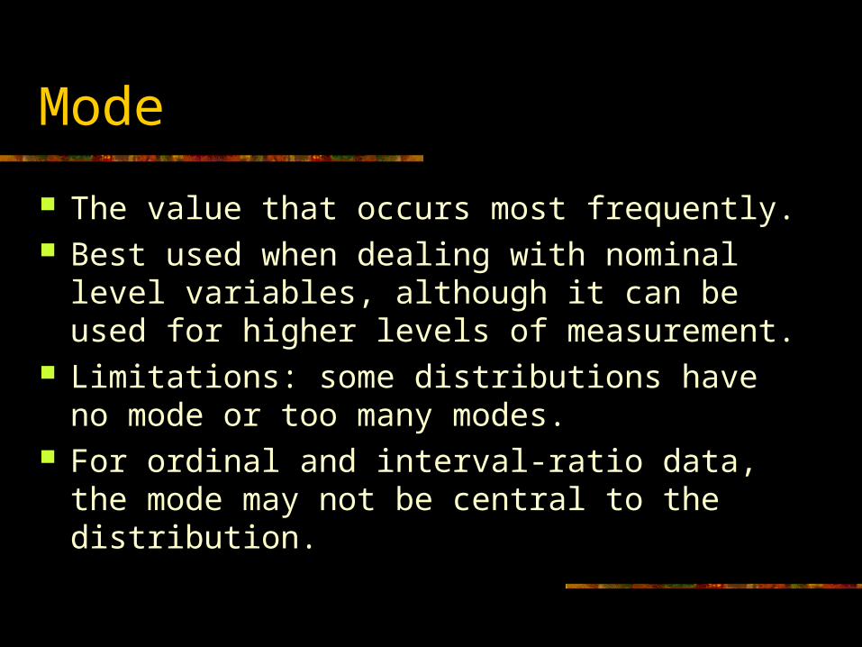
Mode

The value that occurs most frequently. Best used when dealing with nominal level

variables, although it can be used for higher levels of measurement.

Limitations: some distributions have no mode or too many modes.

For ordinal and interval-ratio data, the mode may not be central to the distribution.

Median

Always represents the exact center of a distribution of scores.

The median is the score of the case where half of the cases are higher and half of the cases are lower. If the median family income is $30,000, half of the families make less than $30,000 and half make more.

Median

Before finding the median, the scores must be arranged in order from lowest to highest or highest to lowest.

When the number of cases is odd, the central case is the median [(N+1)/2 case].

Median

When the number of cases is even, the median is the arithmetic average of the two central cases [the mean of case N/2 and case (N/2+1)].

The median can be calculated for ordinal and interval-ratio data.

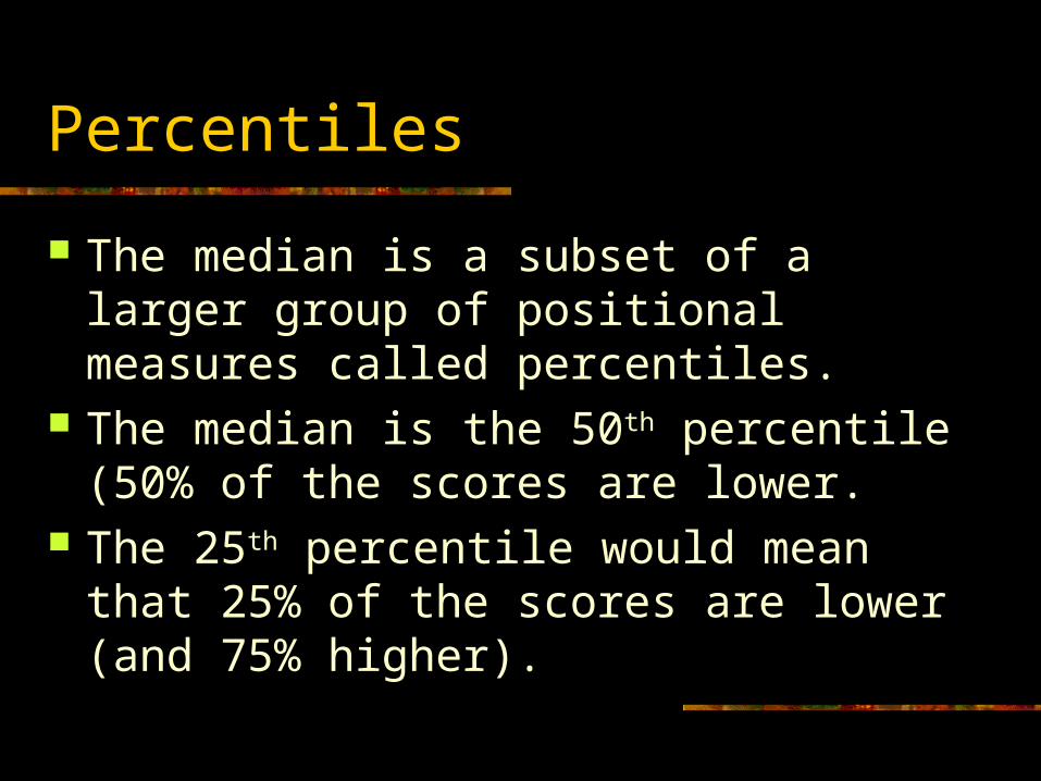
Percentiles

The median is a subset of a larger group of positional measures called percentiles.

The median is the 50th percentile (50% of the scores are lower.

The 25th percentile would mean that 25% of the scores are lower (and 75% higher).

Percentiles

Deciles divide distribution into ten equal segments. The score at the first decile has 10% of the scores lower, the second decile had 20% of the scores lower, etc.

Quartiles divide the distribution into quarters.

The second quartile, the fifth decile and the median are all the same value.

Mean

The calculation of the mean is straightforward: add the scores and divide by the number of scores.

Mathematical formula:

scores ofnumber the

scores; theofsummation the

mean; the

where

N

X

X

N

XX

i

i

Characteristics of the Mean

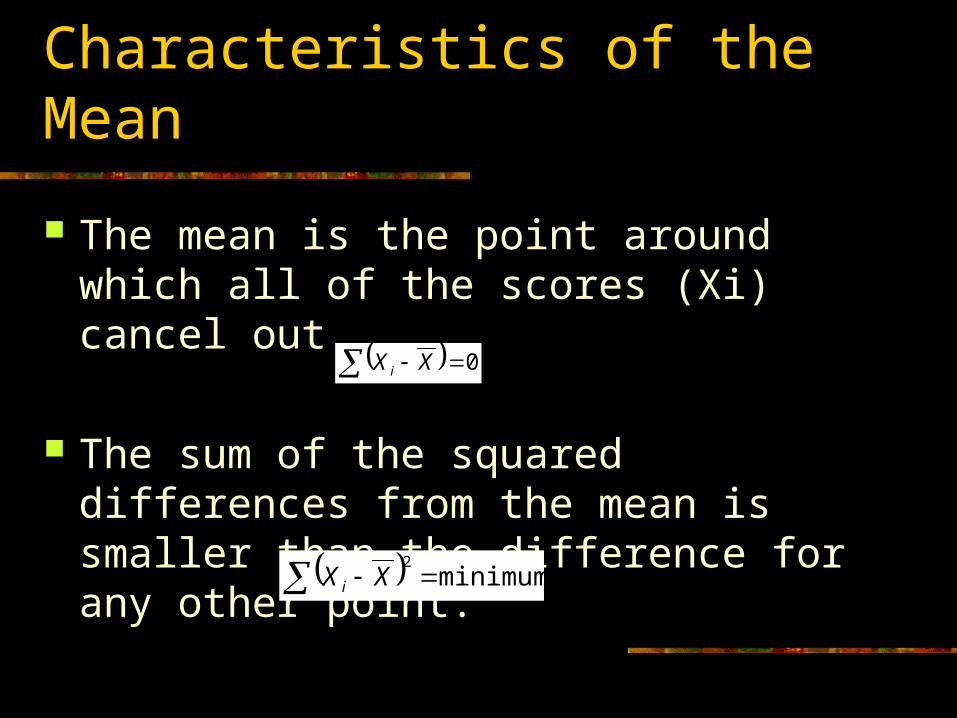
The mean is the point around which all of the scores (Xi) cancel out.

The sum of the squared differences from the mean is smaller than the difference for any other point.

0XX i

minimum 2

XX i

Characteristics of the Mean

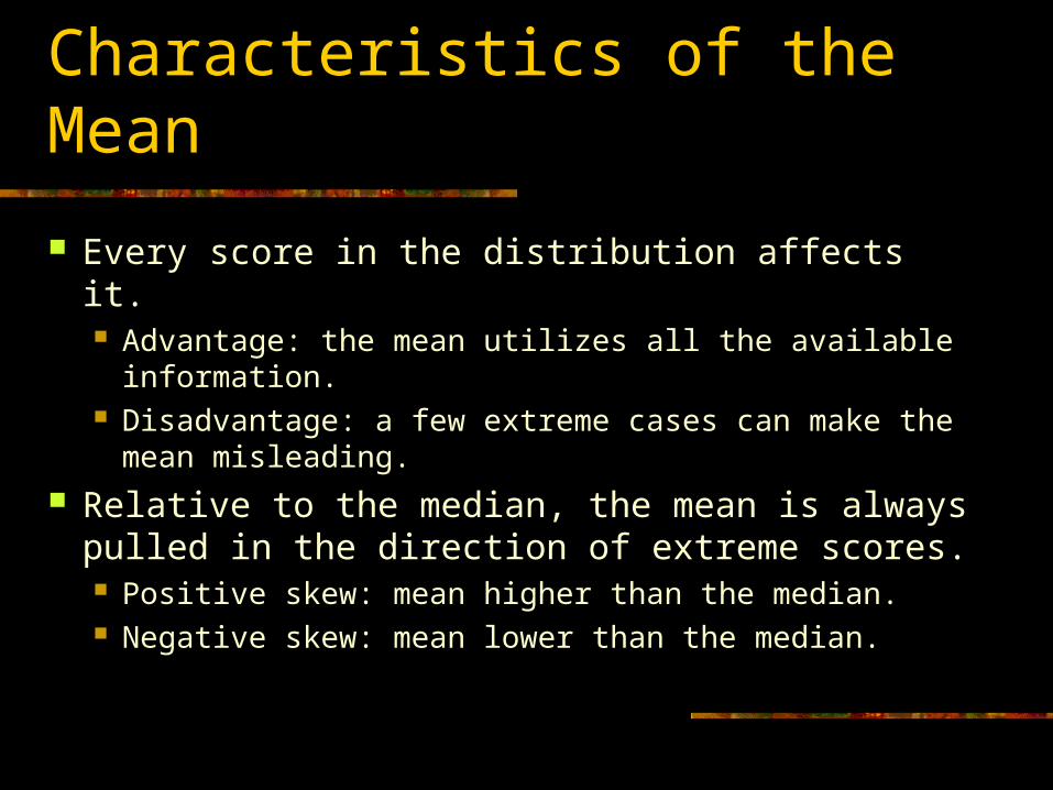
Every score in the distribution affects it. Advantage: the mean utilizes all the available

information. Disadvantage: a few extreme cases can make the

mean misleading. Relative to the median, the mean is always

pulled in the direction of extreme scores. Positive skew: mean higher than the median. Negative skew: mean lower than the median.

Rules for the Selection of Measures of Central Tendency

Use the mode when: Variables are measured at the nominal level. You want a quick and easy measure for ordinal or

interval measures. You want to report the most common score.

Use the median when: Variables are measured at the ordinal level. Variables measured at the interval-ratio level have

highly skewed distributions. You want to report the central score.

Rules for the Selection of Measures of Central Tendency

Use the mean when: Variables are measured at the interval-ratio

level (except for highly skewed distributions). You want to report the most typical score.

The mean is the fulcrum that exactly balances all scores.

You anticipate additional statistical analyses.

Grouped Median

If you do not have raw data, but have only the grouped frequency distribution, assume all cases are evenly distributed across each interval and estimate the median with the following formula.

Grouped Median

median containing intervalin frequency f

intervallower next in cases ofnumber cf

cases ofnumber N

widthintervali

limit realLower L

Median

:where

)%50(

b

Md

f

cfNiLMd b

Grouped Mean

If you do not have raw data, but only have the grouped frequency distribution, assign the midpoint to each interval, multiply the midpoint by the number of cases in each interval, sum, and divide by the number of cases to get an estimate of the mean.

N

fxX igrouped

Example: ModeStatistics

7-PT SCALE PARTY IDENTIFICATION

0

1729 2

1088 2

1690 2

1382 1

1132 2

1237 2

1536 1

1263 2

1531 2

1490 2

2656 2

1533 2

2213 2

2224 2

1577 2

1383 2

2198 2

2120 2

1999 2

1935 1

2445 1

1772 2

1695 2

1255 1a

1776 1

YEAR OF STUDY1948

1952

1954

1956

1958

1960

1962

1964

1966

1968

1970

1972

1974

1976

1978

1980

1982

1984

1986

1988

1990

1992

1994

1996

1998

2000

Valid

N

Mode

Multiple modes exist. The smallest value is showna.

Example: MedianReport

7-PT SCALE PARTY IDENTIFICATION

3.00 1729

3.00 1088

3.00 1690

2.00 1382

3.00 1132

3.00 1237

2.00 1536

3.00 1263

3.00 1531

3.00 1490

3.00 2656

3.00 1533

3.00 2213

3.00 2224

3.00 1577

3.00 1383

4.00 2198

3.00 2120

4.00 1999

3.00 1935

3.00 2445

4.00 1772

3.00 1695

3.00 1255

3.00 1776

3.00 42859

YEAR OF STUDY1952

1954

1956

1958

1960

1962

1964

1966

1968

1970

1972

1974

1976

1978

1980

1982

1984

1986

1988

1990

1992

1994

1996

1998

2000

Total

Median N

Example: MeanReport

7-PT SCALE PARTY IDENTIFICATION

3.47 1729

3.45 1088

3.66 1690

3.40 1382

3.55 1132

3.51 1237

3.26 1536

3.47 1263

3.45 1531

3.48 1490

3.60 2656

3.55 1533

3.61 2213

3.49 2224

3.52 1577

3.45 1383

3.77 2198

3.62 2120

3.82 1999

3.59 1935

3.71 2445

3.92 1772

3.68 1695

3.65 1255

3.73 1776

3.59 42859

YEAR OF STUDY1952

1954

1956

1958

1960

1962

1964

1966

1968

1970

1972

1974

1976

1978

1980

1982

1984

1986

1988

1990

1992

1994

1996

1998

2000

Total

Mean N

Example: Mean

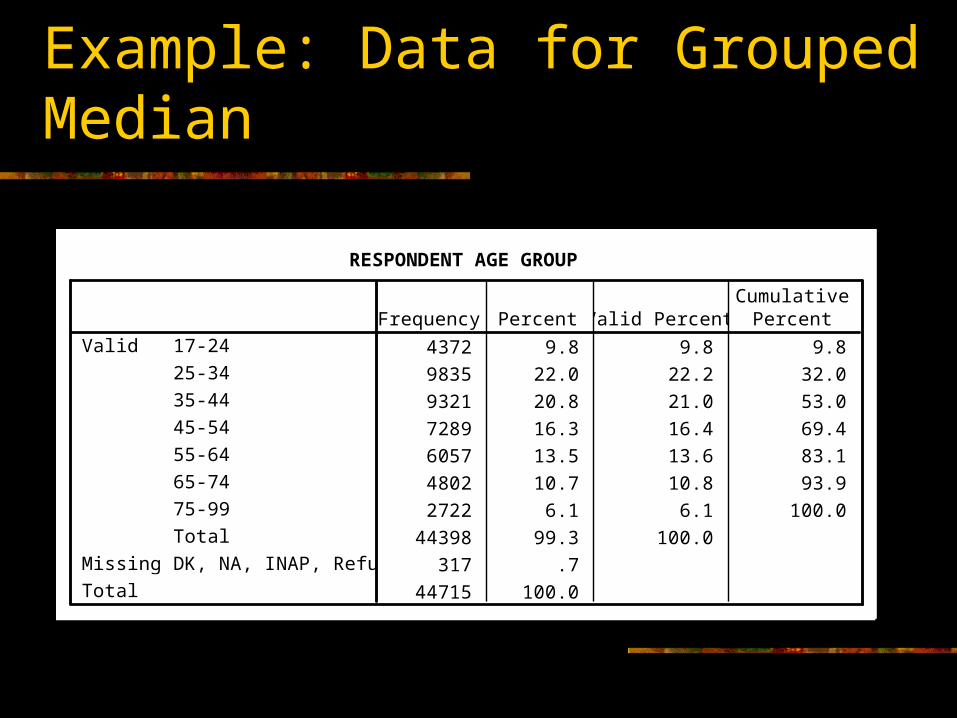
Example: Data for Grouped Median

RESPONDENT AGE GROUP

4372 9.8 9.8 9.8

9835 22.0 22.2 32.0

9321 20.8 21.0 53.0

7289 16.3 16.4 69.4

6057 13.5 13.6 83.1

4802 10.7 10.8 93.9

2722 6.1 6.1 100.0

44398 99.3 100.0

317 .7

44715 100.0

17-24

25-34

35-44

45-54

55-64

65-74

75-99

Total

Valid

DK, NA, INAP, RefusedMissing

Total

Frequency Percent Valid PercentCumulative

Percent

Example: Group Mean – NES 1948-2000

RESPONDENT AGE GROUP Valid CumulativeMidpoint x Midpoint Frequency Percent Percent FrequencyValid 17-24 20.5 4372 9.8 9.8 89626

25-34 29.5 9835 22.2 32.0 290132.535-44 39.5 9321 21.0 53.0 368179.545-54 49.5 7289 16.4 69.4 360805.555-64 59.5 6057 13.6 83.1 360391.565-74 69.5 4802 10.8 93.9 33373975-84 79.5 2722 6.1 100.0 216399Total 44398 100.0 2019273

Group Mean 45.48117

Example: Group Median – NES 1948-2000

RESPONDENT AGE GROUPLower Real Valid Cumulative Limit Frequency Percent PercentValid 17-24 16.5 4372 9.8 9.8

25-34 24.5 9835 22.2 32.035-44 34.5 9321 21.0 53.0 Interval with Median45-54 44.5 7289 16.4 69.455-64 54.5 6057 13.6 83.165-74 64.5 4802 10.8 93.975-84 74.5 2722 6.1 100.0Total 44398 100.0

lower real limit (L) 34.5interval width (i) 10number of cases (N) 44398cumulative frequency below (cfb) 14207interval frequency (f) 9321

Md = L+ [i*(50%*N-cfb)/f]Md = 34.5+ [10*(50%*44398-14207)/9321]Md = 34.5+ [10*(7992)/9321]Md = 34.5+ 8.57Md = 43.07