DISCOVERING MOTIFS IN SPATIAL-TIME SERIES SEISMIC DATASETS

Murillo Guignoni Dutra

Dissertacao de Mestrado apresentada ao Pro-grama de Pos-graduacao em Engenharia deProducao e Sistemas, Centro Federal deEducacao Tecnologica Celso Suckow da Fon-seca CEFET/RJ, como parte dos requisitosnecessarios a obtencao do tıtulo de mestre.

Orientadores:Eduardo Soares OgasawaraFabio Andre Machado Porto

Rio de Janeiro,

Julho 2016

Discovering Motifs in Spatial-Time Series Seismic Datasets

Dissertacao de Mestrado em Engenharia de Producao e Sistemas, Centro Federal de

Educacao Tecnologica Celso Suckow da Fonseca, CEFET/RJ.

Murillo Guignoni Dutra

Aprovada por:

Presidente, Prof. Eduardo Soares Ogasawara, D.Sc. (orientador)

Prof. Fabio Andre Machado Porto, D.Sc. (co-orientador)

Prof. Leonardo Silva de Lima, D.Sc.

Prof. Florent Masseglia, Dr.

Rio de Janeiro,

Julho 2016

ii

Ficha catalográfica elaborada pela Biblioteca Central do CEFET/RJ

D978 Dutra, Murillo Guignoni Discovering motifs in spatial-time series seismic datasets /

Murillo Guignoni Dutra.—2016. 47f. : il.(algumas color.) , grafs. , tabs. ; enc. Dissertação (Mestrado) Centro Federal de Educação

Tecnológica Celso Suckow da Fonseca , 2016. Bibliografia : f. 41-47 Orientador : Eduardo Soares Ogasawara Coorientador : Fabio Andre Machado Porto 1. Prospecção sísmica. 2. Mineração de dados (computação). 3.

Processos estocásticos. 4. Sismologia - Modelos matemáticos. I. Ogasawara, Eduardo Soares (Orient.). II. Porto, Fabio Andre Machado (Coorient.). III. Título.

CDD 550.34

iii

ABSTRACT

Discovering Motifs in Spatial-Time Series Seismic Datasets

Murillo Guignoni Dutra

Advisors:Eduardo Soares OgasawaraFabio Andre Machado Porto

Abstract of dissertation submitted to Programa de Pos-graduacao em Engenharia de Producaoe Sistemas - Centro Federal de Educacao Tecnologica Celso Suckow da Fonseca CEFET/RJ aspartial fulfillment of the requirements for the degree of master.

Discovering motifs in time series data has been widely explored by recent researches. It isbeing motivated by the potential to identify relevant implicit information. Many time series datamining techniques were adapted to solve the problem regarding motif identification in time series.However, when it comes to spatial-time series, it is possible to observe an open gap according tothe literature review. This work proposes a new approach to discover motif in spatial-time series.It is based on combining spatial-time series into a single time series. Then, Random Projectionalgorithm is applied in this transformed time series to identify candidate spatial-time motifs. Fi-nally, candidates are aggregate and validate according to spatial-time constraints. The approachis evaluated in a seismic dataset. Identified motifs were able to identify seismic horizons, which isan important characteristics in seismic analysis.

Key-words:Motifs; Spatial-Time Series; Seismic.

Rio de Janeiro,

Julho, 2016

iv

Contents

I Introduction 1

II Seismic Background 5

II.1 Data acquisition 6

II.2 Seismic Processing 7

II.3 Seismic Interpretation 7

II.4 Final Comments 8

III Time series data mining background 9

III.1 Time series 9

III.2 Subsequence 9

III.3 Sliding Windows 10

III.4 Spatial-time series 10

III.5 Normalization 11

III.6 Symbolic Aggregation Approximation (SAX) 11

III.7 Motif 12

III.7.1 Brute-force algorithm 13

III.7.2 Random Projection algorithm 13

III.8 Ranking motifs 15

III.9 Final Comments 16

IV Related Works 17

V Combined Series Approach 21

V.1 Problem Definition 21

V.2 Combined Series Approach 23

V.2.1 Normalization & SAX Indexing 24

V.2.2 Partition of Spatial-Time Series and Motif Discovery Algorithm 25

V.2.3 Aggregate Motifs and Evaluate Spatial Time Constraints 27

V.2.4 Rank Spatial-Time Motifs 28

v

V.3 CSA Algorithm 29

VI Experimental Evaluation 30

VI.1 Dataset description 30

VI.2 Experiments 32

VII Conclusion 36

Appendix 37

I Ranking Function for Seismic Dataset 38

I.1 Clustering Background 38

I.2 Ranking Function 39

References 40

vi

List of Figures

I.1 Seismic Dataset 3

II.1 seismic dataset Example 6

II.2 Seismic Reflection Example - Source: https://krisenergy.com/company/about-oil-

and-gas/exploration/ 7

III.1 An example of a time series with sub-sequence and sliding windows concepts 10

III.2 Symbolic Indexing methods 12

III.3 Collision matrix construction 15

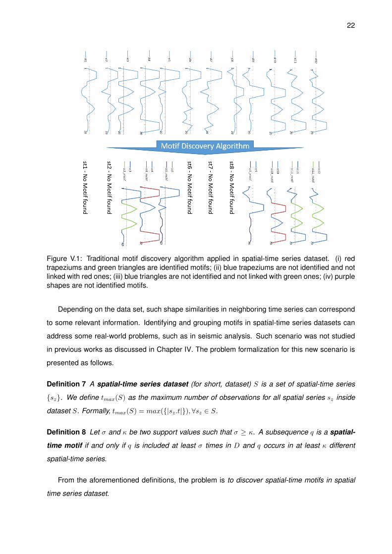
V.1 Traditional motif discovery algorithm applied in spatial-time series dataset. (i) red

trapeziums and green triangles are identified motifs; (ii) blue trapeziums are not

identified and not linked with red ones; (iii) blue triangles are not identified and not

linked with green ones; (iv) purple shapes are not identified motifs. 22

V.2 Spatial-time series motif discovery process 23

V.3 Toy dataset (a); Graphical representation (b) 24

V.4 Toy dataset partitioned into blocks 25

V.5 Motif Discovery Algorithm to Combined Series 26

V.6 Aggregated Motifs (a); Support constraint (σ) (b); Spatial constraint (κ)(c) 28

VI.1 seismic dataset - Inline 401 31

VI.2 Inline 401 data distribution 31

VI.3 Mapped Horizons 32

VI.4 SAX with alpha = 4 33

VI.5 Combined series experiment result 35

I.1 Clustering 39

vii

List of Tables

III.1 Hamming distance example 13

IV.1 Comparison of Works regarding motif discovering in times series 20

V.1 Global Occurrences - Combined Series x Traditional Method 27

VI.1 Input Parameters 33

VI.2 Block 33

VI.3 Summary of Identified Spatial-Time Motifs 34

VI.4 Best ranked Spatial-time motif 34

VI.5 Ranking Result 34

1

Chapter I Introduction

Under the data deluge scenario, Data Scientists are continuously being stressed to provide

new ways for efficiently collecting, storing, processing, and organizing large amount of data [Tsai

et al., 2015]. We are immersed in a scenario with massive databases from many sources, types,

and formats. However, such scenario opens a set of research opportunities involving knowledge

discovery [Han, 2006; Shumway R. H. & Stoffer, 2006]. In this context, many phenomena can

be observed and organized as a sequence of observations in time line that can be modelled as

time series. There are many uses and applications for time series analysis. It can represent

the behavior of process variables in a industrial plant, the price of stocks in financial market,

economic and social indicators, medicine, weather conditions, and anything that can be measured

and registered in time.

One of the areas that is being very often explored in time series analysis is finding patterns

[Patel et al., 2002]. Patterns are sub-sequences of time series that can indicate some special

properties or behaviors that are potentially important and should be more carefully observed and

analysed [Han et al., 2007]. Pattern can be used in many applications, such as in medicine, to

evaluate the health of a person based on an electrocardiogram; in financial market, to correlate

stock prices, currencies, and commodities price; in weather prediction, to analyze meteorological

phenomena that occurs recursively; in industry, to use the best combination of production factors

to get the maximum efficiency with minimum cost based on historical records; in geophysics,

to analyze seismograph data to detect anomalies, subsoil properties, and even earthquakes or

tsunamis.

Finding those patterns may be a hard task to do without computational support. Trying to do

it by graphical or visual analysis limits accuracy and restricts our ability to analyze only small set

of data [Keogh and Kasetty, 2003]. On the other hand, the advances of computational resources

provided the possibility to handle and process large amount of data in a feasible time with accuracy

[Last et al., 2004]. Such scenario encouraged many researches in this area targeting to execute

the pattern finding task more efficient [Agrawal et al., 1993].

One way to find patterns in time series is when a previously known behavior, represented as

a sub-sequence, is used as a parameter to find similar occurrences in the analyzed time series

[Ding et al., 2008]. It is known as pattern matching queries. It is done basically comparing the

2

known sub-sequence to all sub-sequences in data set analyzed.

Another important time series pattern analysis is the identification of a particular behavior in

time series that occurs a significant number of times but it is not previously known. This phe-

nomenon is denominated motif. Identifying motifs is being intensely explored with different tech-

niques, methods, and algorithms, such as finding motifs of a particular length [Li and Lin, 2010],

finding motifs without any constraint (parameter free algorithms) [Madicar et al., 2014], finding

motifs in multivariate time series [Minnen et al., 2007].

Motif discovery has important applications in many areas of knowledge. The term was origi-

nally coined in biology and represents the amino-acid sequence pattern in that context [Staden,

1989]. After that, the motif concept was generalized and expanded due to the possibility to under-

stand and identify some specific behaviors based on patterns observed in the time series data.

It allowed to apply these concepts to another interesting areas as weather prediction [McGovern

et al., 2011], financial [Jiang et al., 2008], wind generation [Fan and Kamath, 2015], sea water

level [Li and Nallela, 2009], image recognition [Chi et al., 2012], seismic amplitude [Cassisi et al.,

2013].

The basic difference between traditional pattern mining and motif discovery is the parameter for

computing similarity between sub-sequences [Lonardi and Patel, 2002]. While for pattern mining

the objective is to find all sub-sequences in a the time series that are equal to a candidate frequent

sub-sequence, in motif discovery, the goal is to find a set of similar sub-sequences that occurs in

relevant number of times. Such threshold may vary according to the method used to find motifs.

A more complex problem involves the identification of patterns according to time and space.

Many very important phenomena are modeled as a set of time series, where each one of them

has an associated position in space. Such scenarios are known as spatial-time series and they

bring challenges in both data management and in methods for knowledge discovery.

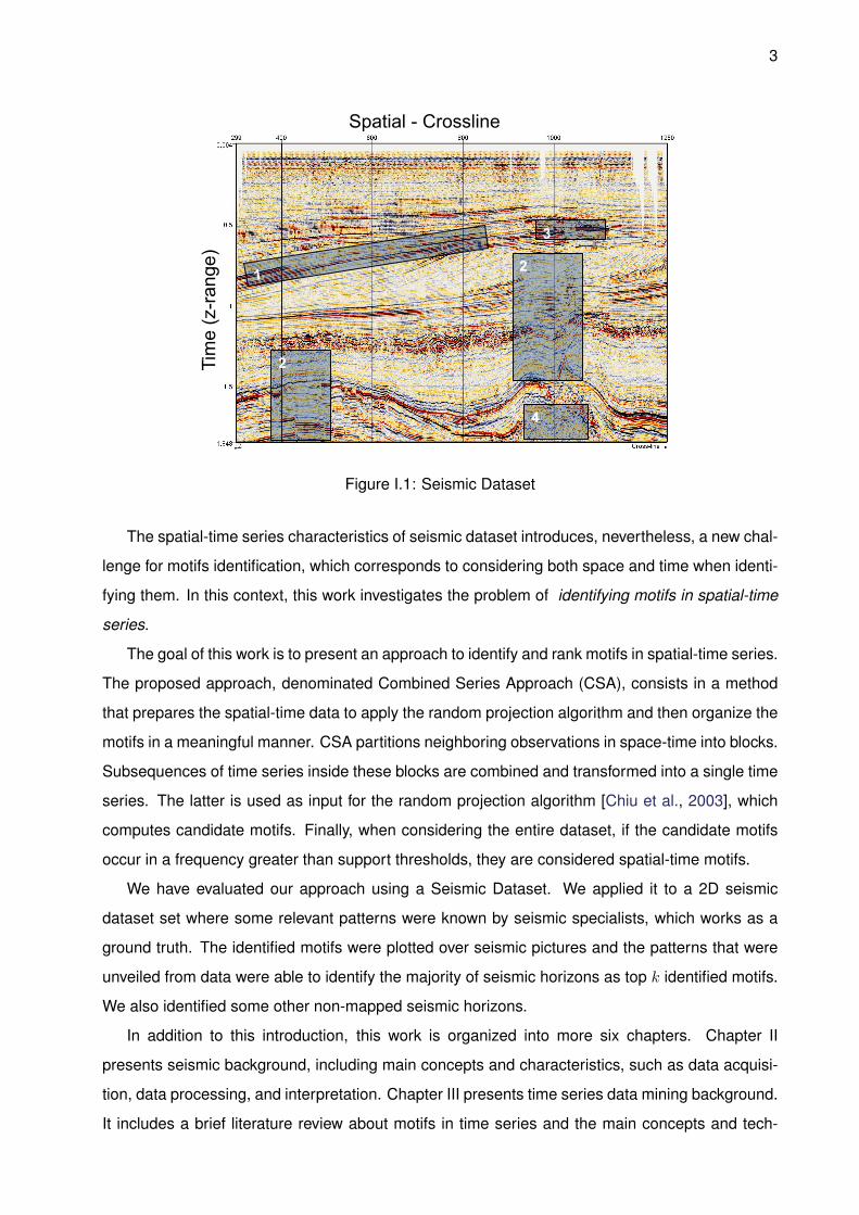
The seismic dataset is a good example of a spatial-time series. Figure I.1 presents a seismic

shot. Each x is associated to a position in space and each y is associated to a time, which is

also related to a depth in subsoil. A value in each x and y position is a seismic observation. The

way in which observable values as spatially and timely distributed may give important information

about soil. In Figure I.1 there are some important soil properties: (1) horizons; (2) faults; (3) gas

reservoir, (4) igneous rock. Although specialists aim in find these patterns, they are not known

beforehand and they need to be inspected and studied using visualization techniques and other

complementary analysis.

3

Spatial - Crossline

Tim

e (z

-rang

e)3

2

2

4

Figure I.1: Seismic Dataset

The spatial-time series characteristics of seismic dataset introduces, nevertheless, a new chal-

lenge for motifs identification, which corresponds to considering both space and time when identi-

fying them. In this context, this work investigates the problem of identifying motifs in spatial-time

series.

The goal of this work is to present an approach to identify and rank motifs in spatial-time series.

The proposed approach, denominated Combined Series Approach (CSA), consists in a method

that prepares the spatial-time data to apply the random projection algorithm and then organize the

motifs in a meaningful manner. CSA partitions neighboring observations in space-time into blocks.

Subsequences of time series inside these blocks are combined and transformed into a single time

series. The latter is used as input for the random projection algorithm [Chiu et al., 2003], which

computes candidate motifs. Finally, when considering the entire dataset, if the candidate motifs

occur in a frequency greater than support thresholds, they are considered spatial-time motifs.

We have evaluated our approach using a Seismic Dataset. We applied it to a 2D seismic

dataset set where some relevant patterns were known by seismic specialists, which works as a

ground truth. The identified motifs were plotted over seismic pictures and the patterns that were

unveiled from data were able to identify the majority of seismic horizons as top k identified motifs.

We also identified some other non-mapped seismic horizons.

In addition to this introduction, this work is organized into more six chapters. Chapter II

presents seismic background, including main concepts and characteristics, such as data acquisi-

tion, data processing, and interpretation. Chapter III presents time series data mining background.

It includes a brief literature review about motifs in time series and the main concepts and tech-

4

niques that support the motif discovering processes. Chapter IV presents the Related Works.

Chapter V presents CSA. It formalizes the problem and describes the algorithm to find motifs in

spatial-time series. Chapter VI describes and explains the experiments that were made using

seismic dataset. Finally, Chapter VII concludes and discusses opportunities for improving our

results.

5

Chapter II Seismic Background

An overview regarding seismic analysis is presented in this chapter. Such explanation is nec-

essary to understand the experiment proposed and the effectiveness evaluation of the presented

method in this work. It is not intended to be a complete survey about seismic. The main objective

is to provide readers with a baseline knowledge that is used in experimental evaluation.

Seismology is the scientific study of the propagation of elastic waves through the Earth. Seis-

mic waves produced by explosions (or vibrating controlled sources) are commonly produced to

explore underground. Data is collected through sensors that measure waves responses from

deep Earth layers. The interpretation of observations made at the surface provides useful infor-

mation about the structure and composition of the inaccessible areas in great depths. Almost all

knowledge about under wells and underground mines in deep depths comes from geophysical

observations [Zhou, 2014].

Much of the tools and techniques developed for such studies have been applied in academic

research on the nature of the Earth’s interior. However, the breakthrough achieved in geophysical

techniques is mainly due to its heavy use in the exploration of hydrocarbons and minerals. The

development of technologies in the areas of acquisition, processing and interpretation of seismic

data, combined with the study of the relationship between seismic properties, petrophysical prop-

erties, and environmental conditions have made this technique the most adopted exploration tool

and one of the most important in characterization of oil reservoir [Yilmaz, 2001].

The seismic reflection method is based on generating artificial seismic waves through explo-

sives, compressed air guns or other seismic sources and record the reflections from the various

interfaces in the subsurface using as geophones receivers or hydrophones, which are devices

analogous to microphones. The generated wave propagates through the interior of the Earth. The

partial reflected waves are used to find interfaces between layers that have significant contrast

elastic properties. The time of arrival of each reflection are related to the propagation velocities

of the seismic wave in each layer. At first approximation, the recorded amplitude is related to the

acoustic impedance contrast, compressional product of velocity and density of the layers defining

the interface. This method is analogous to imaging the human body using ultrasound. However,

unlike medicine, where the density contrasts are imaged, on seismic exploration, the effect of the

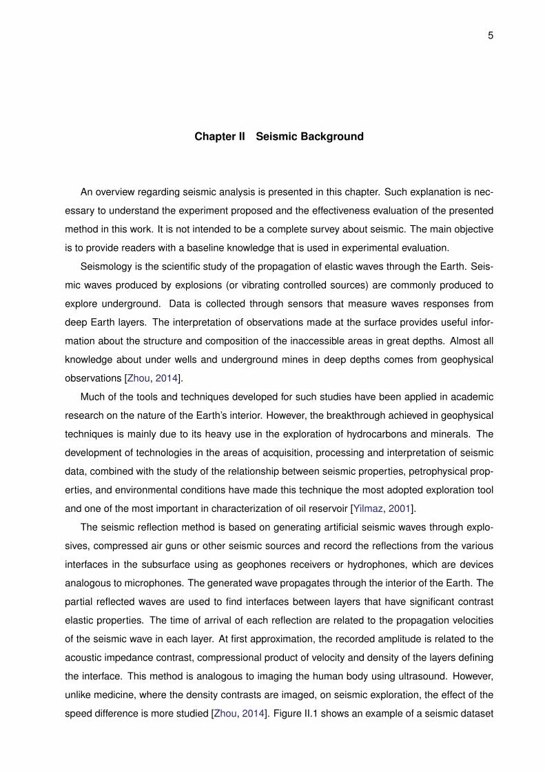
speed difference is more studied [Zhou, 2014]. Figure II.1 shows an example of a seismic dataset

6

represented in a seismic analysis software (OpendTect). Yilmaz [2001] describes the seismic

analysis divided into three parts: data acquisition, seismic processing, and seismic interpreting.

Figure II.1: seismic dataset Example

II.1 Data acquisition

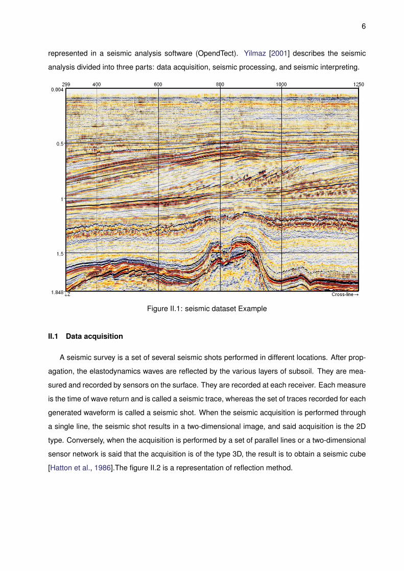
A seismic survey is a set of several seismic shots performed in different locations. After prop-

agation, the elastodynamics waves are reflected by the various layers of subsoil. They are mea-

sured and recorded by sensors on the surface. They are recorded at each receiver. Each measure

is the time of wave return and is called a seismic trace, whereas the set of traces recorded for each

generated waveform is called a seismic shot. When the seismic acquisition is performed through

a single line, the seismic shot results in a two-dimensional image, and said acquisition is the 2D

type. Conversely, when the acquisition is performed by a set of parallel lines or a two-dimensional

sensor network is said that the acquisition is of the type 3D, the result is to obtain a seismic cube

[Hatton et al., 1986].The figure II.2 is a representation of reflection method.

7

Figure II.2: Seismic Reflection Example - Source: https://krisenergy.com/company/about-oil-and-gas/exploration/

II.2 Seismic Processing

In case of seismic shot, for example, the geophones are spaced every 50 meters and seis-

mic trace was recorded for 4 seconds. As the seismic source is located in the center, possible

reflectors appear distorted due to the displacement of receptors in relation to the seismic source.

It is also observed the existence of a high level of noise in the signal. For the seismic acquisition

to represent more realistically the geological structure of the subsurface, seismic shots must be

adjusted. This adjustment process is called seismic processing and imaging. It is said that after

the acquired data are properly processed it creates a 2D seismic line or 3D seismic cube.

II.3 Seismic Interpretation

The seismic interpretation comprehends the analysis of the images processed for exploration,

characterization, and monitoring of oil reservoirs. These analyzes are very important to the oil

8

industry, since it is from such analysis that the location of oil or gas reservoirs exploration is

decided. Recently, it has also been used to monitor seismic reservoir to monitor oil exploitation.

In seismic exploration, seismic images are analyzed in detail by interpreters for signs that may

indicate the presence of hydrocarbons. The seismic interpretation assumes that the contrast of

acoustic impedance in the subsurface represented by seismic images has its origin in changes

in the composition of the different layers of rocks. An important characteristic in understanding

the underground consists in identifying seismic horizons. A horizon can be identified in the traces

as an amplitude pattern in the vertical neighborhood. Moreover, such pattern occurs in the trace

repeatedly where the horizon is defined [Zhou, 2014]. Real horizons can be represented by traces

of the volume by a small set of vertically contiguous voxels. Seismic horizons help to understand

the region. Some of them delimit the base and the top of a possible reservoirs [Zhou, 2014].

II.4 Final Comments

In this Chapter, we presented some seismic background which are relevant in understanding

the use case scenario adopted in this dissertation. It was possible to see the importance of

some characteristics in seismic analysis such as finding horizons, faults and potential hydrocarbon

concentration zones. The focus of the analysis presented in this work is in finding seismic horizons.

9

Chapter III Time series data mining background

In this chapter, we introduce some background in time series data mining. We present a

formalization and introduce some basic related concepts, including the definition for: time series,

sub-sequences, and sliding windows. In addition, motif discovering mining process is described,

including the activities of: normalization, data indexing, similarity measurements, and discovery

algorithms.

III.1 Time series

A time series is a collection of observations of a phenomenon along a time-line [Hamilton,

1994]. Time series analysis is a large field of study and was intensively developed with the ad-

vances of computational resources. This allowed for handling a massive quantity of data [Cryer

and Kellet, 1986]. The time series analysis is normally based on statistical references, including

the extraction of time series properties such as average, median, variance, and distribution [Wei,

1994]. Formally:

Definition 1 According to Box et al. [2008], a time series t is an ordered sequence of values in

time , where each ti is a value, |t| = m is the number of elements in t and tm is the most recent

value in t.

t =< t1, t2, · · · , tm >, ti ∈ R

III.2 Subsequence

A subsequence is a sample of a time series. It enables the analysis of a subset of the data

to evaluate some local properties [Chiu et al., 2003]. A subsequence has a defined length and is

necessarily smaller than the time series. Formally:

Definition 2 According to Lonardi and Patel [2002], the p-th sub sequence of size n in a time

series t, represented as tp,n, is an ordered sequence of values < tp, tp+1, . . ., tp+n−1 >, where

|tp,n| = n and 1 ≤ p ≤ |t| − n.

tp,n = subseq(t, p, n)

10

III.3 Sliding Windows

Sliding windows consists in extracting all possible subsequences of a time series [Lampert

et al., 2008]. The sliding windows produces a set o subsequences with the same length. Such

concept is widely used for time series analysis to make comparison between subsequences to

find similarities between them [Van Hoan and Exbrayat, 2013]. Formally:

Definition 3 A Sliding Windows [Keogh and Lin, 2005] is a function sw(t, n) with arguments t

and n that produces a matrix W of size (|t| − n+ 1) by n that contains all sub sequences of size n

of time series t. Each line wi in W is a sub sequence of t of size n. Given W = sw(t, n), ∀wi ∈W ,

wi = ti,n.

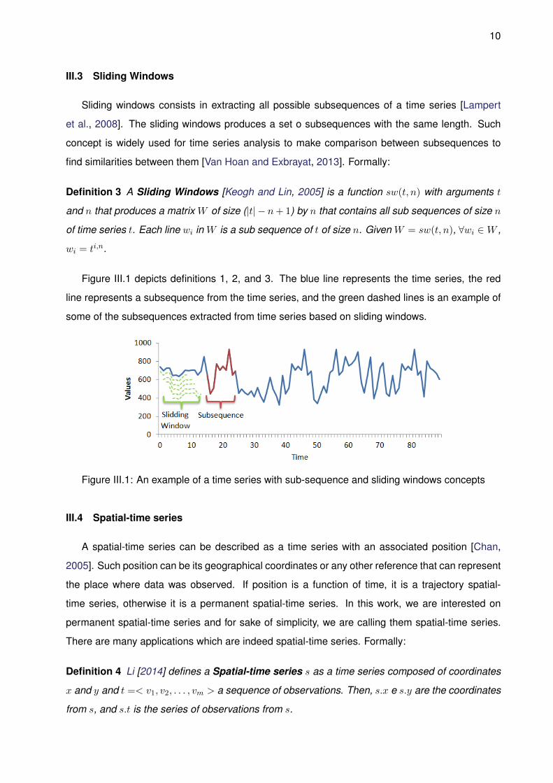
Figure III.1 depicts definitions 1, 2, and 3. The blue line represents the time series, the red

line represents a subsequence from the time series, and the green dashed lines is an example of

some of the subsequences extracted from time series based on sliding windows.

Figure III.1: An example of a time series with sub-sequence and sliding windows concepts

III.4 Spatial-time series

A spatial-time series can be described as a time series with an associated position [Chan,

2005]. Such position can be its geographical coordinates or any other reference that can represent

the place where data was observed. If position is a function of time, it is a trajectory spatial-

time series, otherwise it is a permanent spatial-time series. In this work, we are interested on

permanent spatial-time series and for sake of simplicity, we are calling them spatial-time series.

There are many applications which are indeed spatial-time series. Formally:

Definition 4 Li [2014] defines a Spatial-time series s as a time series composed of coordinates

x and y and t =< v1, v2, . . . , vm > a sequence of observations. Then, s.x e s.y are the coordinates

from s, and s.t is the series of observations from s.

11

III.5 Normalization

There are some different methods to compare time series, such as morphological comparison

[Loh et al., 2000]. To apply such methods to compare them, it is necessary to verify some proper-

ties, such as scale. In this way, normalization becomes a fundamental step in data preprocessing

to enable the effectiveness of time series comparison methods. One of the most common normal-

ization methods is the amplitude normalization or z-score [Keogh and Ratanamahatana, 2005].

As result of this normalization method, the normalized time series has zero as average and one

as standard deviation. The equation III.1 presents how to normalize a time series.

zm =(tm − µt)

σt(III.1)

where µt is the average and σt is the standard deviation of the time series.

III.6 Symbolic Aggregation Approximation (SAX)

One of the data preprocessing activities in motif discovery consists in representing data in a

manageable way [Lin et al., 2007]. Such representation is a complex task and depends on data

domain [Shieh and Keogh, 2008]. In time series context, data is usually a continuous numerical

value. For motif discovery, processing directly numerical representation is not an efficient way to

adopt [Daw et al., 2003]. Some discretization methods, such as symbolic representation (also

known as indexing) has been proposed. It consists basically in represent a range of values as a

symbol. All values in such range are replaced by that symbol according to a defined alphabet.

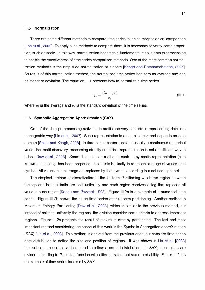
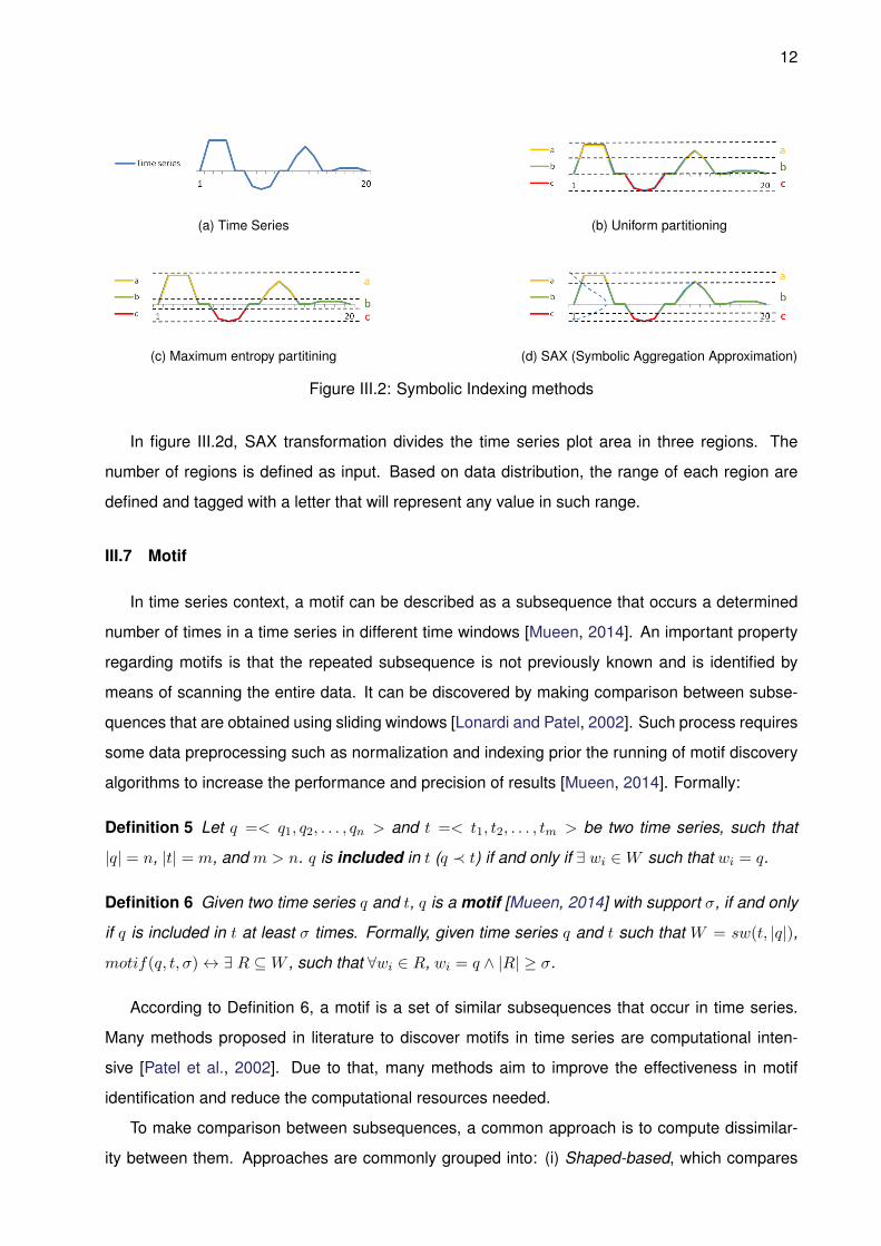
The simplest method of discretization is the Uniform Partitioning which the region between

the top and bottom limits are split uniformly and each region receives a tag that replaces all

value in such region [Keogh and Pazzani, 1998]. Figure III.2a is a example of a numerical time

series. Figure III.2b shows the same time series after uniform partitioning. Another method is

Maximum Entropy Partitioning [Daw et al., 2003], which is similar to the previous method, but

instead of splitting uniformly the regions, the division consider some criteria to address important

regions. Figure III.2c presents the result of maximum entropy partitioning. The last and most

important method considering the scope of this work is the Symbolic Aggregation approXimation

(SAX) [Lin et al., 2003]. This method is derived from the previous ones, but consider time series

data distribution to define the size and position of regions. It was shown in Lin et al. [2003]

that subsequence observations trend to follow a normal distribution. In SAX, the regions are

divided according to Gaussian function with different sizes, but same probability. Figure III.2d is

an example of time series indexed by SAX.

12

(a) Time Series (b) Uniform partitioning

(c) Maximum entropy partitining (d) SAX (Symbolic Aggregation Approximation)

Figure III.2: Symbolic Indexing methods

In figure III.2d, SAX transformation divides the time series plot area in three regions. The

number of regions is defined as input. Based on data distribution, the range of each region are

defined and tagged with a letter that will represent any value in such range.

III.7 Motif

In time series context, a motif can be described as a subsequence that occurs a determined

number of times in a time series in different time windows [Mueen, 2014]. An important property

regarding motifs is that the repeated subsequence is not previously known and is identified by

means of scanning the entire data. It can be discovered by making comparison between subse-

quences that are obtained using sliding windows [Lonardi and Patel, 2002]. Such process requires

some data preprocessing such as normalization and indexing prior the running of motif discovery

algorithms to increase the performance and precision of results [Mueen, 2014]. Formally:

Definition 5 Let q =< q1, q2, . . . , qn > and t =< t1, t2, . . . , tm > be two time series, such that

|q| = n, |t| = m, and m > n. q is included in t (q ≺ t) if and only if ∃ wi ∈W such that wi = q.

Definition 6 Given two time series q and t, q is a motif [Mueen, 2014] with support σ, if and only

if q is included in t at least σ times. Formally, given time series q and t such that W = sw(t, |q|),

motif(q, t, σ)↔ ∃ R ⊆W , such that ∀wi ∈ R, wi = q ∧ |R| ≥ σ.

According to Definition 6, a motif is a set of similar subsequences that occur in time series.

Many methods proposed in literature to discover motifs in time series are computational inten-

sive [Patel et al., 2002]. Due to that, many methods aim to improve the effectiveness in motif

identification and reduce the computational resources needed.

To make comparison between subsequences, a common approach is to compute dissimilar-

ity between them. Approaches are commonly grouped into: (i) Shaped-based, which compares

13

the shape of subsequences; (ii) Edit-Based, which counts the minimum number of interactions to

transform one subsequence in another, (iii) Feature-based, which extracts properties from subse-

quences to compare them using another metric, and (iv) Structure-based, which try to find high

level structures in subsequences to compare them using a global scale [Esling and Agon, 2012].

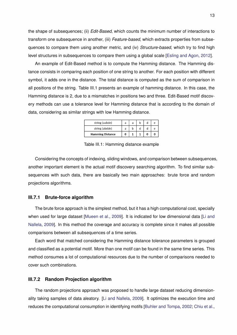
An example of Edit-Based method is to compute the Hamming distance. The Hamming dis-

tance consists in comparing each position of one string to another. For each position with different

symbol, it adds one in the distance. The total distance is computed as the sum of comparison in

all positions of the string. Table III.1 presents an example of hamming distance. In this case, the

Hamming distance is 2, due to a mismatches in positions two and three. Edit-Based motif discov-

ery methods can use a tolerance level for Hamming distance that is according to the domain of

data, considering as similar strings with low Hamming distance.

Table III.1: Hamming distance example

Considering the concepts of indexing, sliding windows, and comparison between subsequences,

another important element is the actual motif discovery searching algorithm. To find similar sub-

sequences with such data, there are basically two main approaches: brute force and random

projections algorithms.

III.7.1 Brute-force algorithm

The brute force approach is the simplest method, but it has a high computational cost, specially

when used for large dataset [Mueen et al., 2009]. It is indicated for low dimensional data [Li and

Nallela, 2009]. In this method the coverage and accuracy is complete since it makes all possible

comparisons between all subsequences of a time series.

Each word that matched considering the Hamming distance tolerance parameters is grouped

and classified as a potential motif. More than one motif can be found in the same time series. This

method consumes a lot of computational resources due to the number of comparisons needed to

cover such combinations.

III.7.2 Random Projection algorithm

The random projections approach was proposed to handle large dataset reducing dimension-

ality taking samples of data aleatory. [Li and Nallela, 2009]. It optimizes the execution time and

reduces the computational consumption in identifying motifs [Buhler and Tompa, 2002; Chiu et al.,

14

2003]. In random projection, the data preprocessing is similar to brute-force method. It includes

indexing and sliding windows.

With the set of words resulted from such data preprocessing, each symbolic subsequence

is inserted in a subsequences matrix. Each line index corresponds to the initial position of sub-

sequence in time axis. The next step is to build the collision matrix which is used to indicated

potential motifs in the time series. The collision matrix is initially null and has the same quantity of

lines and columns that correspond to the total number of subsequences identified. The collision

matrix is built from the random projection process where two columns of the subsequence matrix

are randomly selected and mask and for each position in mapped as a hash structure that has as

input the symbolic values that correspond to position of selected columns. If two subsequences

has the same symbolic value in the mask position then it is placed in hash structure.

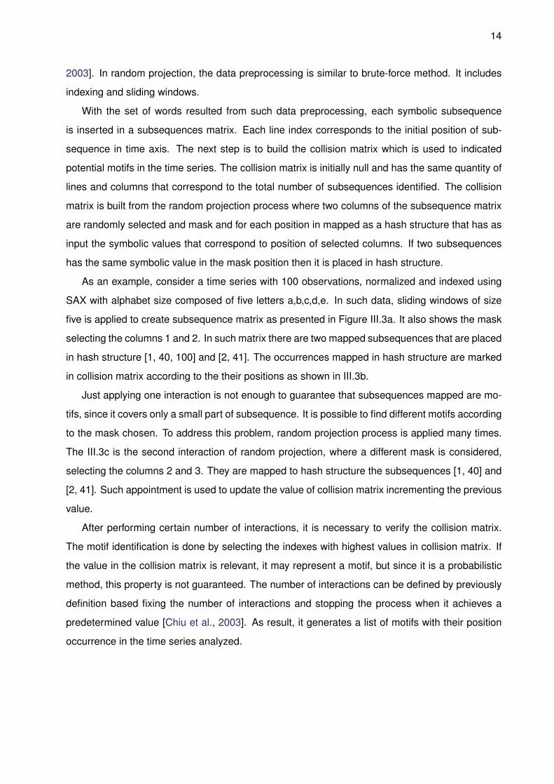
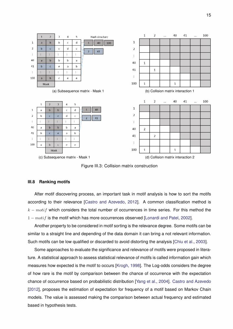
As an example, consider a time series with 100 observations, normalized and indexed using

SAX with alphabet size composed of five letters a,b,c,d,e. In such data, sliding windows of size

five is applied to create subsequence matrix as presented in Figure III.3a. It also shows the mask

selecting the columns 1 and 2. In such matrix there are two mapped subsequences that are placed

in hash structure [1, 40, 100] and [2, 41]. The occurrences mapped in hash structure are marked

in collision matrix according to the their positions as shown in III.3b.

Just applying one interaction is not enough to guarantee that subsequences mapped are mo-

tifs, since it covers only a small part of subsequence. It is possible to find different motifs according

to the mask chosen. To address this problem, random projection process is applied many times.

The III.3c is the second interaction of random projection, where a different mask is considered,

selecting the columns 2 and 3. They are mapped to hash structure the subsequences [1, 40] and

[2, 41]. Such appointment is used to update the value of collision matrix incrementing the previous

value.

After performing certain number of interactions, it is necessary to verify the collision matrix.

The motif identification is done by selecting the indexes with highest values in collision matrix. If

the value in the collision matrix is relevant, it may represent a motif, but since it is a probabilistic

method, this property is not guaranteed. The number of interactions can be defined by previously

definition based fixing the number of interactions and stopping the process when it achieves a

predetermined value [Chiu et al., 2003]. As result, it generates a list of motifs with their position

occurrence in the time series analyzed.

15

(a) Subsequence matrix - Mask 1 (b) Collision matrix interaction 1

(c) Subsequence matrix - Mask 1 (d) Collision matrix interaction 2

Figure III.3: Collision matrix construction

III.8 Ranking motifs

After motif discovering process, an important task in motif analysis is how to sort the motifs

according to their relevance [Castro and Azevedo, 2012]. A common classification method is

k − motif which considers the total number of occurrences in time series. For this method the

1−motif is the motif which has more occurrences observed [Lonardi and Patel, 2002].

Another property to be considered in motif sorting is the relevance degree. Some motifs can be

similar to a straight line and depending of the data domain it can bring a not relevant information.

Such motifs can be low qualified or discarded to avoid distorting the analysis [Chiu et al., 2003].

Some approaches to evaluate the significance and relevance of motifs were proposed in litera-

ture. A statistical approach to assess statistical relevance of motifs is called information gain which

measures how expected is the motif to occurs [Krogh, 1998]. The Log-odds considers the degree

of how rare is the motif by comparison between the chance of occurrence with the expectation

chance of occurrence based on probabilistic distribution [Yang et al., 2004]. Castro and Azevedo

[2012], proposes the estimation of expectation for frequency of a motif based on Markov Chain

models. The value is assessed making the comparison between actual frequency and estimated

based in hypothesis tests.

16

Another important approach that may be used to rank motifs is to cluster the occurrences

of each motif and compute some quality measures. The general approach for clustering are

described as follows.

III.9 Final Comments

In this Chapter, we discussed the main concepts and techniques used to develop the CSA such

the basic concepts in time series analysis regarding motif identification such, subsequence and

Sliding Windows. We defined the spatial-time series as a time series with a position associated.

We presented the data treatment by normalization and SAX indexing process. We explored the

motif definition and described the brute-force and Random Projection algorithm. At last, brought a

ranking motifs description and methods presented in literature.

17

Chapter IV Related Works

This chapter presents a brief review regarding the most relevant works performed in time series

motif discovery. The first approach regarding motif discovery in time series was proposed in

Lonardi and Patel [2002]. In their approach, it is necessary to choose some parameters, such

as motif length, size of SAX alphabet, and similarity tolerance between subsequences to classify

them as a motif. It also describes the concept of k-motifs, which corresponds to the k most

significant motifs.

Lonardi and Patel [2002] proposed a brute-force algorithm called EMMA (Enumeration of Mo-

tifs through Matrix Approximation) . Brute-force algorithms have quadratic complexity for pro-

cessing. Since then, the task to identify motifs in time series has been widely explored. Recent

researches focus on either improving the quality or reducing computational costs to find them.

Chiu et al. [2003], for example, proposed a optimized method, extended from Buhler and Tompa

[2002], aiming to reduce the computational cost to identify motifs.

Considering the exact motif discovery approach, some specific method to address the dimen-

sionality and motif length problem were proposed. For univariate data with fixed-length motif, Jiang

et al. [2008] proposed an efficient motif discovery algorithm PMDGS (P-Motif Discovery based on

Grid Structure) that processes data streams. Mueen et al. [2009] proposed an exact time se-

ries motif discovery algorithm called MK (Mueen-Keogh) and observed that MK was faster than

brute-force presented by Lonardi and Patel [2002]. Narang and Bhattacherjee [2010] introduce

the Par-MK, Par-MK-SLB, and Par-MK-DLB. They are parallel multi-threaded algorithms for exact

motif discover that focus on load balancing. Mueen et al. [2011] proposed a disk-aware algorithm

to exact identify motifs in large time series databases. Cassisi et al. [2013] applies an exact time

series motif discovery technique to study recurrent patterns in seismic amplitude time series of the

Etna 2011 periodic eruptive activity. Chi and Wang [2013] introduced a method based on cloud

model theory to extract the top k-motifs. Truong and Anh [2015] proposed a fast method for motif

discovery in time series based on Dynamic Time Warping distance.

When it comes to approximated motif discovery methods, they aim to reduce the complexity

and consequently the computational cost. Some work proposed approaches to improve the accu-

racy and efficiency of Random Projection Algorithm proposed in Chiu et al. [2003]. For univariate

data with fixed-length motif, Lin et al. [2007] created a new symbolic representation for time series

18

(SAX) for indexing. Mohammad and Nishida [2009] proposed two algorithms called MCFull and

MCInc that addresses constrained motif discovery problem. Castro and Azevedo [2010] addresses

motif discovery problem as an approximate top k frequent subsequence discovery problem. Lin

et al. [2010] presented an approach that uses subseries joins to get similarity among subseries of

the time series. Armstrong and Drewniak [2011] developed the algorithm MD-RP for unsupervised

motif discovering in time series. Narang and Bhattcherjee [2011] designed the new sequential and

parallel Motif discovery and data de-duplication algorithms based on bloom filters.

For univariate data and variable-length motif discovery, Wilson et al. [2007] proposed the Motif

Tracking Algorithm (MTA) that uses a small number of parameters based on implementation of the

Bell immune memory theory. Yankov et al. [2007] presented a novel algorithm that discover motifs

in time series with invariance to uniform scaling. This enables to reduce parameters such as motif

length. In Nunthanid et al. [2011], a new motif discovery algorithm that do not requires motif length

parameter called VLMD is introduced. Such algorithm automatically returns motif lengths from all

possible sliding window lengths reducing a set of possibilities of the sliding window lengths. Nun-

thanid et al. [2012] presented the k-Best Motif Discovery (kBMD), a new time series motif discovery

algorithm that is free of parameter produces a set of the best motif that are ranked by a scoring

function based on similarity of motif locations and shapes. Mueen [2013] proposed the MOEN, an

exact free-parameter algorithm to enumerate motifs that is faster than brute-force approach due

to a novel bound on the similarity function that uses only linear space. Mohammad and Nishida

[2014a] proposed an extension of the MK algorithm called MK++ to handle multiple motifs of vari-

able lengths considering maximum overlap of subsequences. Mohammad and Nishida [2014b]

presented a new algorithm, derived from MK++ to find the top K similar subsequence pairs at

multiple lengths efficiently using scale invariant distance functions.

In the approximated approach for univariate time series with variable-length, Tang and Liao

[2008] presented a new k-motif-based algorithm that is able to discover approximated motif with

no need to define the length of motif. Li and Lin [2010] proposed the Sequitur, a new approximated

approach based on grammar induction considering variable-length time series motif discovery with

improvement of discovering hierarchical structure, regularity and grammar from data. Mohammad

et al. [2012] proposed the G-Tex algorithm that can discover multiple motifs of multiple lengths

with good performance. Truong and Anh [2013] developed the EP-BIRCH algorithm that is more

efficient than MK algorithm finding motifs in large time series datasets and has low sensibility

regarding the input parameters as motif-length.

In multivariate time series with fixed motif length, Tanaka and Uehara [2003] and Tanaka et al.

[2005] showed how to dynamically determine the optimum period length using the Minimum De-

scription Length (MDL) principle and apply the method to the multidimensional time-series trans-

19

forming into one dimensional time-series using the Principal Component Analysis. Liu et al. [2005]

proposed heuristic approach that can significantly improve the quality of motifs in m-dimensional

time series. Lam et al. [2011] proposed two algorithms for solving multivariate time series called

nmotif and kmotif. McGovern et al. [2011] introduced an approach to mining multidimensional mo-

tif in temporal streams of real-world data. Son and Anh [2016] proposed two new algorithms for

motif discovery in time series data, first based on R-tree and the other is based on dimensionality

reduction through Skyline index.

In multivariate time series with fixed-length, Vahdatpour et al. [2009] proposed a new model

based on Random Projection to find approximately motif in multivariate time series data by com-

bining motifs discovered and grouping them. Wang et al. [2010] developed the AMG method

to list the motifs candidates by scanning the entire series and then filling a matrix for similarity

comparison to verify the real motif. Son and Anh [2012] presented a R*-tree together with early

abandoning based approach that stores Minimum Bounding Rectangles (MBR) of data in mem-

ory. Regarding the variable-length, the work of Minnen et al. [2007] proposed a method based on

Random Projections for motif finding high density regions in the space of time series.

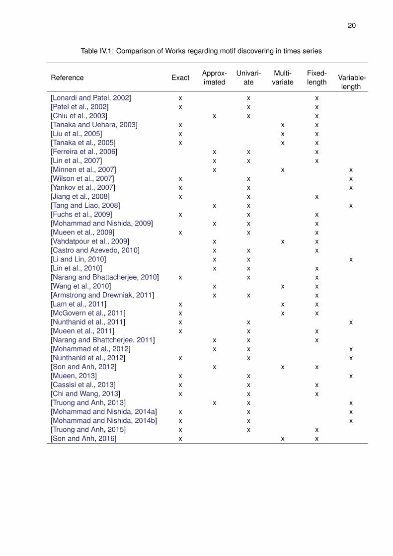
There are many works that proposes algorithm, methods and approaches to handle with motif

discovery task with different characteristic such exactness, dimensionality and motif length. Ta-

ble IV.1 summaries a comparison between works that contributed to motif discover, according to

the following properties: exactness of algorithm (Exact or Approximated); dimensionality of data

(Univariate or Multivariate); and length of motif (Fixed-length or Variable-length).

20

Table IV.1: Comparison of Works regarding motif discovering in times series

Reference ExactApprox-imated

Univari-ate

Multi-variate

Fixed-length

Variable-length

[Lonardi and Patel, 2002] x x x[Patel et al., 2002] x x x[Chiu et al., 2003] x x x[Tanaka and Uehara, 2003] x x x[Liu et al., 2005] x x x[Tanaka et al., 2005] x x x[Ferreira et al., 2006] x x x[Lin et al., 2007] x x x[Minnen et al., 2007] x x x[Wilson et al., 2007] x x x[Yankov et al., 2007] x x x[Jiang et al., 2008] x x x[Tang and Liao, 2008] x x x[Fuchs et al., 2009] x x x[Mohammad and Nishida, 2009] x x x[Mueen et al., 2009] x x x[Vahdatpour et al., 2009] x x x[Castro and Azevedo, 2010] x x x[Li and Lin, 2010] x x x[Lin et al., 2010] x x x[Narang and Bhattacherjee, 2010] x x x[Wang et al., 2010] x x x[Armstrong and Drewniak, 2011] x x x[Lam et al., 2011] x x x[McGovern et al., 2011] x x x[Nunthanid et al., 2011] x x x[Mueen et al., 2011] x x x[Narang and Bhattcherjee, 2011] x x x[Mohammad et al., 2012] x x x[Nunthanid et al., 2012] x x x[Son and Anh, 2012] x x x[Mueen, 2013] x x x[Cassisi et al., 2013] x x x[Chi and Wang, 2013] x x x[Truong and Anh, 2013] x x x[Mohammad and Nishida, 2014a] x x x[Mohammad and Nishida, 2014b] x x x[Truong and Anh, 2015] x x x[Son and Anh, 2016] x x x

21

Chapter V Combined Series Approach

V.1 Problem Definition

The motif discovery approaches presented in literature review basically propose to solve the

problem considering time series. In the context of spatial-time series where exists a neighborhood

relationship among time-series, we observe a more complex scenario due to spatial constraints.

In order to highlight how challenging the problem is, consider a set of spatial-time series

dataset where each spatial-time series has a position. Such scenario is depicted in Figure V.1. If

we apply to this scenario a known motif discovery method, such as Random Projection Algorithm,

on each spatial-time series, we can observe that no motif is found in five spatial-time series. Also,

even when some motifs are identified, considering the entire data set, those motifs are not fully

explored. It is possible to observe that similar shapes appearing in neighboring spatial time series

are not identified as motifs when running the algorithm on each time series separately.

22

Figure V.1: Traditional motif discovery algorithm applied in spatial-time series dataset. (i) redtrapeziums and green triangles are identified motifs; (ii) blue trapeziums are not identified and notlinked with red ones; (iii) blue triangles are not identified and not linked with green ones; (iv) purpleshapes are not identified motifs.

Depending on the data set, such shape similarities in neighboring time series can correspond

to some relevant information. Identifying and grouping motifs in spatial-time series datasets can

address some real-world problems, such as in seismic analysis. Such scenario was not studied

in previous works as discussed in Chapter IV. The problem formalization for this new scenario is

presented as follows.

Definition 7 A spatial-time series dataset (for short, dataset) S is a set of spatial-time series

{sz}. We define tmax(S) as the maximum number of observations for all spatial series sz inside

dataset S. Formally, tmax(S) = max({|sz.t|}),∀sz ∈ S.

Definition 8 Let σ and κ be two support values such that σ ≥ κ. A subsequence q is a spatial-

time motif if and only if q is included at least σ times in D and q occurs in at least κ different

spatial-time series.

From the aforementioned definitions, the problem is to discover spatial-time motifs in spatial

time series dataset.

23

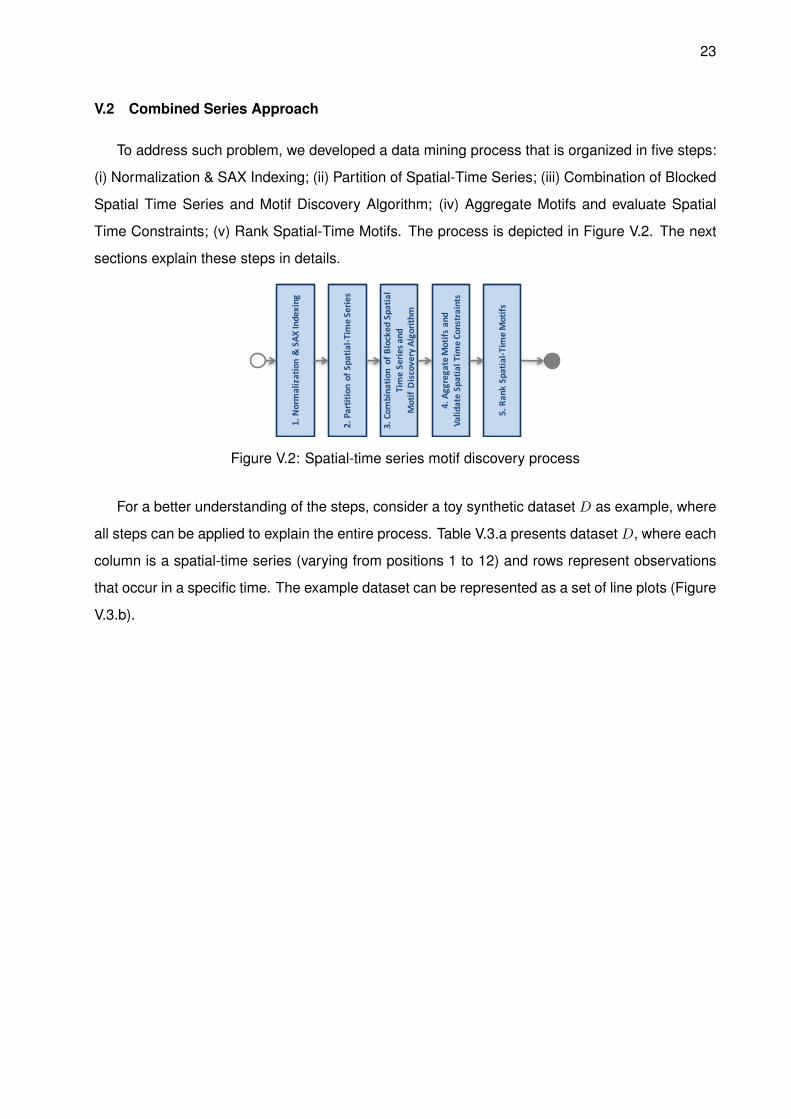
V.2 Combined Series Approach

To address such problem, we developed a data mining process that is organized in five steps:

(i) Normalization & SAX Indexing; (ii) Partition of Spatial-Time Series; (iii) Combination of Blocked

Spatial Time Series and Motif Discovery Algorithm; (iv) Aggregate Motifs and evaluate Spatial

Time Constraints; (v) Rank Spatial-Time Motifs. The process is depicted in Figure V.2. The next

sections explain these steps in details.

2.PartitionofSpatia

l-Tim

eSerie

s

4.AggregateMotifsand

ValidateSpatialTim

eConstraints

3.Com

binatio

nofBlockedSpatia

lTimeSerie

sand

MotifDiscoveryAlgorith

m

5.RankSpatial-T

imeMotifs

1.Normalization&SAX

Indexing

Figure V.2: Spatial-time series motif discovery process

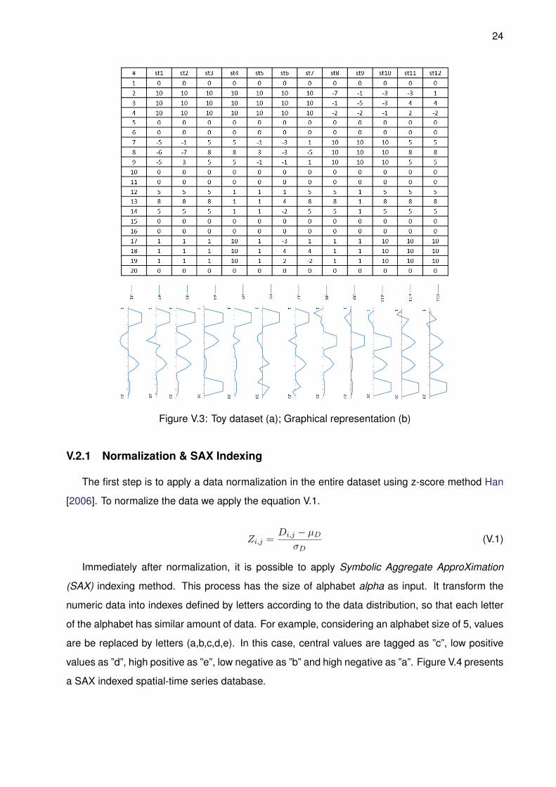
For a better understanding of the steps, consider a toy synthetic dataset D as example, where

all steps can be applied to explain the entire process. Table V.3.a presents dataset D, where each

column is a spatial-time series (varying from positions 1 to 12) and rows represent observations

that occur in a specific time. The example dataset can be represented as a set of line plots (Figure

V.3.b).

24

Figure V.3: Toy dataset (a); Graphical representation (b)

V.2.1 Normalization & SAX Indexing

The first step is to apply a data normalization in the entire dataset using z-score method Han

[2006]. To normalize the data we apply the equation V.1.

Zi,j =Di,j − µD

σD(V.1)

Immediately after normalization, it is possible to apply Symbolic Aggregate ApproXimation

(SAX) indexing method. This process has the size of alphabet alpha as input. It transform the

numeric data into indexes defined by letters according to the data distribution, so that each letter

of the alphabet has similar amount of data. For example, considering an alphabet size of 5, values

are be replaced by letters (a,b,c,d,e). In this case, central values are tagged as ”c”, low positive

values as ”d”, high positive as ”e”, low negative as ”b” and high negative as ”a”. Figure V.4 presents

a SAX indexed spatial-time series database.

25

V.2.2 Partition of Spatial-Time Series and Motif Discovery Algorithm

The second step is to partition the spatial-time series dataset into blocks. Blocks are created

based on sslice (spatial slice) tslice (time slice). sslice is the number of neighbors series inside

each block and tslice is length of subsequences of the spatial time series. In this way, each block

contains sslice · tslice observations.

Considering our example, Figure V.4 depicts the partition of the dataset, where each blue box

corresponds to a block. In this example, the input threshold sslice is 4 and tslice is 10. Since the

dataset has 12 columns and 20 rows, the dataset is divided into 6 blocks.

Figure V.4: Toy dataset partitioned into blocks

Once the partitioning of the data has been applied, each block is used for motif discovery

algorithm. This is an important step in Combined Series Approach to identify motifs in spatial-

time series since it combines observations with different space and time. This partitioning groups

spatial-time series in different positions according to a fixed time window. Another important char-

acteristics of this procedure is to reduce the computational complexity when processing large

datasets.

In each block, we concatenate the spatial-time subsequences into a single time series t. The

concatenation occurs linearizing the block connecting all columns inside the block by the last

element of previous column to first element to next column consideration orientation left-to-right.

After concatenation, the problem becomes a traditional motif discovery problem. It is possible to

directly apply the random projection algorithm to identify time series motifs. Once at least one

motif is found, the step returns a list of motifs and their occurrences that includes the word that

represent the motif and a vector of initial positions where the motif is found.

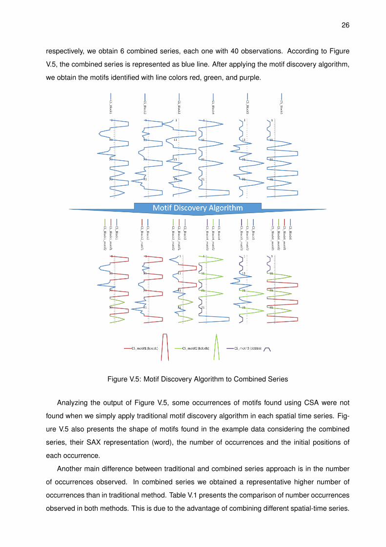
Figure V.5 shows CSA applied to our toy dataset. Considering a sslice and tslice of 4 and 10,

26

respectively, we obtain 6 combined series, each one with 40 observations. According to Figure

V.5, the combined series is represented as blue line. After applying the motif discovery algorithm,

we obtain the motifs identified with line colors red, green, and purple.

Figure V.5: Motif Discovery Algorithm to Combined Series

Analyzing the output of Figure V.5, some occurrences of motifs found using CSA were not

found when we simply apply traditional motif discovery algorithm in each spatial time series. Fig-

ure V.5 also presents the shape of motifs found in the example data considering the combined

series, their SAX representation (word), the number of occurrences and the initial positions of

each occurrence.

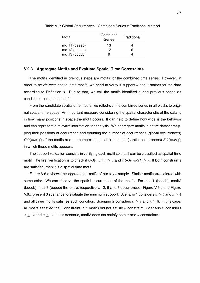
Another main difference between traditional and combined series approach is in the number

of occurrences observed. In combined series we obtained a representative higher number of

occurrences than in traditional method. Table V.1 presents the comparison of number occurrences

observed in both methods. This is due to the advantage of combining different spatial-time series.

27

Table V.1: Global Occurrences - Combined Series x Traditional Method

MotifCombined

SeriesTraditional

motif1 (beeeb) 13 4motif2 (bdedb) 12 6motif3 (bbbbb) 9 4

V.2.3 Aggregate Motifs and Evaluate Spatial Time Constraints

The motifs identified in previous steps are motifs for the combined time series. However, in

order to be de facto spatial-time motifs, we need to verify if support κ and σ stands for the data

according to Definition 8. Due to that, we call the motifs identified during previous phase as

candidate spatial-time motifs.

From the candidate spatial-time motifs, we rolled-out the combined series in all blocks to origi-

nal spatial-time space. An important measure considering the spatial characteristic of the data is

in how many positions in space the motif occurs. It can help to define how wide is the behavior

and can represent a relevant information for analysis. We aggregate motifs in entire dataset map-

ping their positions of occurrence and counting the number of occurrences (global occurrences)

GO(motif) of the motifs and the number of spatial-time series (spatial occurrences) SO(motif)

in which these motifs appears.

The support validation consists in verifying each motif so that it can be classified as spatial-time

motif. The first verification is to check if GO(motif) ≥ σ and if SO(motif) ≥ κ. If both constraints

are satisfied, then it is a spatial-time motif.

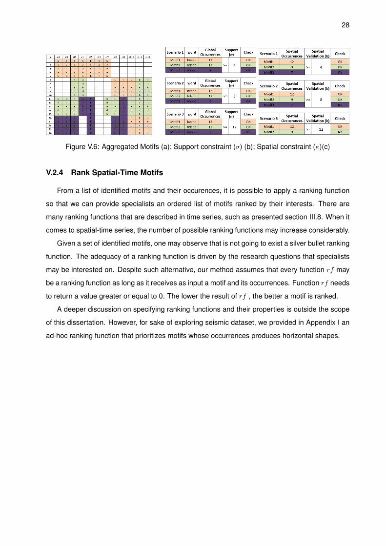
Figure V.6.a shows the aggregated motifs of our toy example. Similar motifs are colored with

same color. We can observe the spatial occurrences of the motifs. For motif1 (beeeb), motif2

(bdedb), motif3 (bbbbb) there are, respectively, 12, 9 and 7 occurrences. Figure V.6.b and Figure

V.6.c present 3 scenarios to evaluate the minimum support. Scenario 1 considers σ ≥ 4 and κ ≥ 4

and all three motifs satisfies such condition. Scenario 2 considers σ ≥ 8 and κ ≥ 8. In this case,

all motifs satisfied the σ constraint, but motif3 did not satisfy κ constraint. Scenario 3 considers

σ ≥ 12 and κ ≥ 12.In this scenario, motif3 does not satisfy both σ and κ constraints.

28

Figure V.6: Aggregated Motifs (a); Support constraint (σ) (b); Spatial constraint (κ)(c)

V.2.4 Rank Spatial-Time Motifs

From a list of identified motifs and their occurences, it is possible to apply a ranking function

so that we can provide specialists an ordered list of motifs ranked by their interests. There are

many ranking functions that are described in time series, such as presented section III.8. When it

comes to spatial-time series, the number of possible ranking functions may increase considerably.

Given a set of identified motifs, one may observe that is not going to exist a silver bullet ranking

function. The adequacy of a ranking function is driven by the research questions that specialists

may be interested on. Despite such alternative, our method assumes that every function rf may

be a ranking function as long as it receives as input a motif and its occurrences. Function rf needs

to return a value greater or equal to 0. The lower the result of rf , the better a motif is ranked.

A deeper discussion on specifying ranking functions and their properties is outside the scope

of this dissertation. However, for sake of exploring seismic dataset, we provided in Appendix I an

ad-hoc ranking function that prioritizes motifs whose occurrences produces horizontal shapes.

29

V.3 CSA Algorithm

The entire data mining process can be summarized by Algorithm 12. It takes as input a spatial-

time series dataset D, a word size w, an alphabet size a, slice and tslide corresponding to spatial

and temporal block sizes, a σ and κ constraints, and, finally a ranking function rf .

1: function STMOTIF(D,w, a, sslice, tslice, σ, κ, rf )

2: Ds ← norm sax(D, a)

3: b← partition(Ds, sslice, tslice)

4: for each bi ∈ b do

5: t← combine(bi)

6: motifs← identify(t, w) ∪motifs

7: end for

8: cand motifs = aggregate(motifs)

9: st motifs = evaluate(cand motifs, σ, κ)

10: topst motifs = rank(st motifs, rf)

11: return topst motifs

12: end function

30

Chapter VI Experimental Evaluation

This chapter addresses experimental evaluation using seismic datasets. Initially, it is pre-

sented an overview about the Netherlands seismic dataset used in this dissertation. Then, both

the methodology and scenarios considered for analysis are presented. Finally, the results are

summarized and evaluated according to the ground truth for the Netherlands seismic dataset.

VI.1 Dataset description

Seismic dataset is a set of spatial-time series. Each spatial-time series has a position in

which the geophone or hydrophone is placed. The experiment proposed in this work consists in

applying CSA in seismic dataset to support seismic interpretation. As presented in chapter II, an

important task in seismic analysis is to identify seismic horizons. They correspond to different

layers in subsoil. The large size of a seismic dataset makes visual analysis conducted by seismic

specialists hard and time consuming.

A seismic dataset, called F3 Block, was selected to evaluate CSA. The dataset was collected

in a region localized in the Dutch sector of the North Sea. Such dataset is a sample that contains

the superior part of seismic of that region. In the bottom part, which is not available for public,

contains the data regarding oil and gas formations. The dataset available is largely studied by

seismic community. Due to that, it was explored by seismic specialists that mapped some relevant

information, such as seismic horizons.

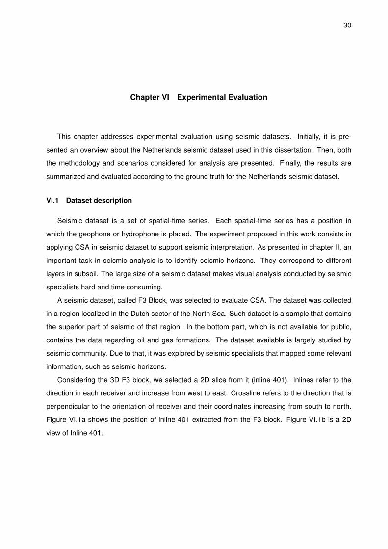
Considering the 3D F3 block, we selected a 2D slice from it (inline 401). Inlines refer to the

direction in each receiver and increase from west to east. Crossline refers to the direction that is

perpendicular to the orientation of receiver and their coordinates increasing from south to north.

Figure VI.1a shows the position of inline 401 extracted from the F3 block. Figure VI.1b is a 2D

view of Inline 401.

31

(a) Inline 401 in block data (b) Inline 401 2D view

Figure VI.1: seismic dataset - Inline 401

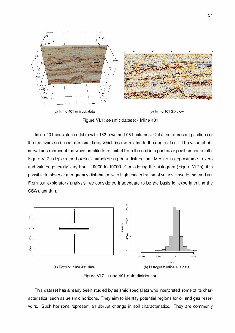
Inline 401 consists in a table with 462 rows and 951 columns. Columns represent positions of

the receivers and lines represent time, which is also related to the depth of soil. The value of ob-

servations represent the wave amplitude reflected from the soil in a particular position and depth.

Figure VI.2a depicts the boxplot characterizing data distribution. Median is approximate to zero

and values generally vary from -10000 to 10000. Considering the histogram (Figure VI.2b), it is

possible to observe a frequency distribution with high concentration of values close to the median.

From our exploratory analysis, we considered it adequate to be the basis for experimenting the

CSA algorithm.

(a) Boxplot Inline 401 data (b) Histogram Inline 401 data

Figure VI.2: Inline 401 data distribution

This dataset has already been studied by seismic specialists who interpreted some of its char-

acteristics, such as seismic horizons. They aim to identify potential regions for oil and gas reser-

voirs. Such horizons represent an abrupt change in soil characteristics. They are commonly

32

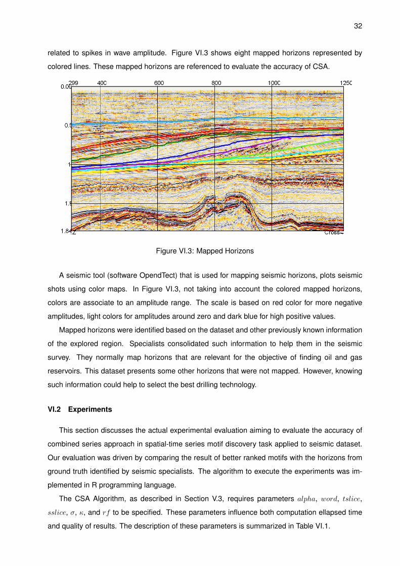
related to spikes in wave amplitude. Figure VI.3 shows eight mapped horizons represented by

colored lines. These mapped horizons are referenced to evaluate the accuracy of CSA.

Figure VI.3: Mapped Horizons

A seismic tool (software OpendTect) that is used for mapping seismic horizons, plots seismic

shots using color maps. In Figure VI.3, not taking into account the colored mapped horizons,

colors are associate to an amplitude range. The scale is based on red color for more negative

amplitudes, light colors for amplitudes around zero and dark blue for high positive values.

Mapped horizons were identified based on the dataset and other previously known information

of the explored region. Specialists consolidated such information to help them in the seismic

survey. They normally map horizons that are relevant for the objective of finding oil and gas

reservoirs. This dataset presents some other horizons that were not mapped. However, knowing

such information could help to select the best drilling technology.

VI.2 Experiments

This section discusses the actual experimental evaluation aiming to evaluate the accuracy of

combined series approach in spatial-time series motif discovery task applied to seismic dataset.

Our evaluation was driven by comparing the result of better ranked motifs with the horizons from

ground truth identified by seismic specialists. The algorithm to execute the experiments was im-

plemented in R programming language.

The CSA Algorithm, as described in Section V.3, requires parameters alpha, word, tslice,

sslice, σ, κ, and rf to be specified. These parameters influence both computation ellapsed time

and quality of results. The description of these parameters is summarized in Table VI.1.

33

Table VI.1: Input Parameters

Parameter Description

alpha Size of alphabet for SAX indexingword Length of motif word

tsliceNumber of rows in the block(subsequence size)

ssliceNumber of columns in the block (numberof spatial time series)

σ Support for Global Occurrence (GO)κ Support of Spatial Occurrence (SO)rf Ranking function (see Appendix I)

Since CSA has a few parameters, we have conducted parameter exploration in two stages. In

the first stage of evaluation, we studied the influence of block orientation by varying both tslice

and sslice. In this stage, we fixed all other parameters. For this first evaluation, parameters were

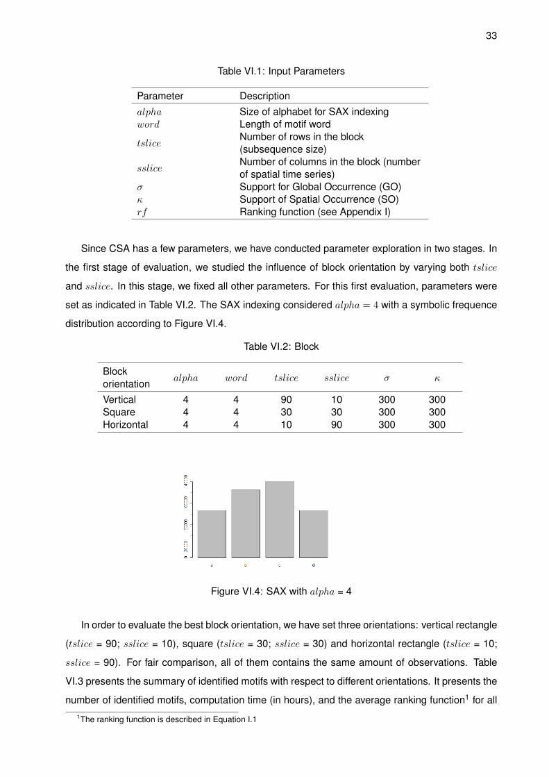
set as indicated in Table VI.2. The SAX indexing considered alpha = 4 with a symbolic frequence

distribution according to Figure VI.4.

Table VI.2: Block

Blockorientation

alpha word tslice sslice σ κ

Vertical 4 4 90 10 300 300Square 4 4 30 30 300 300Horizontal 4 4 10 90 300 300

Figure VI.4: SAX with alpha = 4

In order to evaluate the best block orientation, we have set three orientations: vertical rectangle

(tslice = 90; sslice = 10), square (tslice = 30; sslice = 30) and horizontal rectangle (tslice = 10;

sslice = 90). For fair comparison, all of them contains the same amount of observations. Table

VI.3 presents the summary of identified motifs with respect to different orientations. It presents the

number of identified motifs, computation time (in hours), and the average ranking function1 for all1The ranking function is described in Equation I.1

34

identified motifs. It is possible to observe that horizontal block presented the lowest average rank

and computation time.

Table VI.3: Summary of Identified Spatial-Time Motifs

Blockorientation

Numberof Motifs

Time(hours)

AverageRank

Vertical 314 14.59 0.2463Square 327 17.23 0.2375Horizontal 317 13.36 0.1954

The best ranked motif in the block orientation is the one with the lowest ranking function value

computed by Equation I.1. In order to measure the quality of the ranking function, Equation VI.1

computes the ground-truth error, i.e., RMSE of all observations with respect to the closest seismic

horizons indicated in the ground-truth. Table VI.4 presents the best ranked motif, its ranking func-

tion and ground-truth error for each block orientation. It is possible to observe that better ranked

motif in the horizontal block led to lowest ground-truth error.

rankmotifvalidation =

∑ RMSEcluster(horizon)

(IG+1)∗SO2

GO

ncluster(VI.1)

Table VI.4: Best ranked Spatial-time motif

Blockorientation

stmotifRankingFunction

Ground-truthError

Vertical ddaa 0.0403 0.0866Square aadd 0.0325 0.0914Horizontal aadd 0.0468 0.0821

In stage two, with the best block orientation defined, it possible to evaluate the accuracy of CSA

by varying other parameters. In this stage, we explored varying both alpha and word parameters

from 4 to 8. Table VI.5 presents the ranking function for the best rank motif identified.

Table VI.5: Ranking Result

alphaword 4 5 6 7 8

4 0.0468 0.0407 0.1396 0.2646 0.81725 0.0838 0.1998 1.0202 1.6679 3.51296 0.1654 0.8081 1.5713 3.5870 -7 - 2.2909 - - -8 - - - - -

Considering the results presented in Table VI.5, the best configuration observed is word =

35

4 and alpha = 5. According to Table VI.5, as we increase the word and alpha parameters, the

computed rank also increases. When these parameters imposes more restrictive constraints, the

algorithm may even not find any motif.

We were expecting that with the increase of alpha value, the precision of the results would

have increased. From our observations, it occurred the opposite behavior. We have analyzed that

such behavior was due to the way in which we have configured random projection algorithm. We

have set it to not explore overlapping sliding windows. In other words, all subsequences were

completely independent. This decreased the chances of finding candidate motifs.

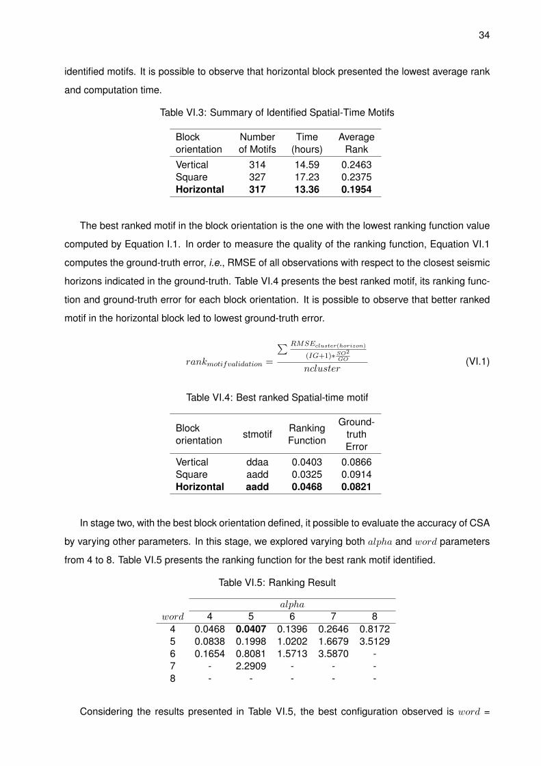
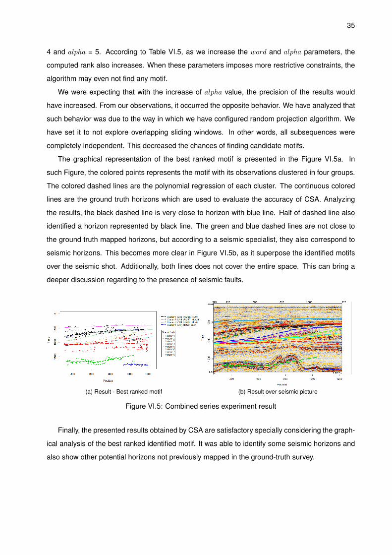
The graphical representation of the best ranked motif is presented in the Figure VI.5a. In

such Figure, the colored points represents the motif with its observations clustered in four groups.

The colored dashed lines are the polynomial regression of each cluster. The continuous colored

lines are the ground truth horizons which are used to evaluate the accuracy of CSA. Analyzing

the results, the black dashed line is very close to horizon with blue line. Half of dashed line also

identified a horizon represented by black line. The green and blue dashed lines are not close to

the ground truth mapped horizons, but according to a seismic specialist, they also correspond to

seismic horizons. This becomes more clear in Figure VI.5b, as it superpose the identified motifs

over the seismic shot. Additionally, both lines does not cover the entire space. This can bring a

deeper discussion regarding to the presence of seismic faults.

(a) Result - Best ranked motif (b) Result over seismic picture

Figure VI.5: Combined series experiment result

Finally, the presented results obtained by CSA are satisfactory specially considering the graph-

ical analysis of the best ranked identified motif. It was able to identify some seismic horizons and

also show other potential horizons not previously mapped in the ground-truth survey.

36

Chapter VII Conclusion

The main contribution of this dissertation is to present an approach for motif identification in

spatial-time series, named Combined Series Approach (CSA). The motif concept, initially cre-

ated in bio-medicine, has been extended to other areas such as time series analysis. Due to the

potential of the technique applied to time series, it became a very interesting theme with large pos-

sibilities for real-world applications. Evaluating the literature, we observe a gap in motif discovery

techniques for handling spatial-time series, which is the focus of this work.

The basic concepts and definitions regarding time series, spatial-time series, and motif dis-

covery in time series were described as background for CSA. Additionally, since the experimental

evaluation is done using seismic dataset, a brief introduction on seismic analysis was presented,

including a discussion on important information to be extract in seismic surveys, such as identifi-

cation of horizons, faults, and reservoirs.

In the literature, many works proposed different approaches for motif discovery in time series

analysis. They are based on similar concepts and techniques. In data preparation some tech-

niques include normalization and Symbolic Aggregation Approximation (SAX). Due to that, for

spatial-time series motifs discovery, CSA was proposed on top of Random Projections.

However, some adaptations were applied to handle with spatial-time series. In fact, CSA is a

data mining process that: prepares spatial-time series; partition and combine them into blocks;

run a motif discovery algorithm in each block; aggregate candidate motifs; evaluate spatial-time

constraints and apply a ranking technique. The constraints aim at evaluating whether a sequence

can be considered a spatial-time motifs, and the rank technique considers the word representation

and the sequence occurrences in spatial-time series.

The experimental evaluation was conducted using a seismic dataset from the Netherlands

offshore, named F3 Block. Such dataset is widely used by researches to evaluate tools and

studies in the seismic interpreting area. The analysis was divided into three stages.

The first stage aims at defining the best shape of the block configuration, established by com-

bining tslice and sslide, to explore seismic dataset. The evaluation measured the accuracy of

each shape when compared both the ranking function and to the ground truth.

In the second stage, alpha and word parameters were tested keeping fixed the remaining

parameters. The best ranked configuration was obtained using word = 4 and alpha = 5. The top

37

ranked motif discovered four shapes. Two of these shapes characterized two seismic horizons,

whereas the other two were not present in the ground-truth, but also corresponded to seismic

horizons, according to a seismic specialist that we have contacted.

Finally, the main contribution of this work was the presentation of a novel approach to identify

motifs in spatial-time series in seismic dataset. CSA was able to identify seismic horizons. The

results of the experimental evaluation indicates a good accuracy when comparing against the

ground truth. Additionally, the discovered motifs were ranked according to their relevance in finding

seismic horizons.

As future works, it is possible to indicate some complementary analysis regarding the varia-

tions of parameters such σ and κ, evaluating the sensibility analysis. Another relevant parameter

whose variation may be interesting to consider is the number of clusters. It can influence directly

in the final ranking analysis. Different motif discovery algorithms, instead of Random Projection,

can be analyzed as well. Moreover, it is also possible to explore different ranking functions that

explore different shapes. Finally, an evaluation regarding overlapping sliding window could be

investigated.

38

Appendix I Ranking Function for Seismic Dataset

This appendices contains a clustering background explaining the main methods for partitioning

data in literature. It also describes the ranking function used to rank the spatial-time motifs. Such

information are important to support the CSA algorithm and experiement analysis.

I.1 Clustering Background

Clustering is an important area in data mining and consists basically in partitioning a set of

data in meaningful groups. It is defined as an unsupervised process since we do not need a

previous labeled data to create the groups [Berkhin, 2006]. The clustering is done according to

a criterion, property or model that can be observed in the data. Fahad et al. [2014] indicates five

categories of clustering methods: (i) partitioning-based, (ii) hierarchical-based, (iii )density-based,

(iv) grid-based, and (v) model-based.

Partitioning-based clustering divides data points into a number k of partitions and each partition

is a cluster. This method has as requirements that each cluster shall have at least one observation

and such observation cannot be in more than one cluster. The most common algorithm is the k-

means [Berkhin, 2006]. Hierarchical-based where data are organized hierarchically according to

the proximity obtained by intermediate nodes. An agglomerative approach, for example, may build

clusterings starting with one observation for each cluster and continuously joining the most similar

ones [Karypis et al., 1999].

Given a set of points in some space, it groups together points that are closely packed together

(points with many nearby neighbors), marking as outliers points that lie alone in low-density re-

gions (whose nearest neighbors are too far away)

Density-based clustering, such as DBSCAN, groups together points that are closely placed

together (points with many nearby neighbors). A Density-based cluster is usually used when data

is irregular, marking as outliers points that lie alone in low-density regions [Ester et al., 1996] .

The grid-based clustering approach uses a multi-resolution grid data structure. It partitions the

object space into a finite number of cells that form a grid structure on which clustering are per-

formed. Since it does not dependent on the number of data objects, it presents a fast processing

time. However, it depends on the number of cells in each dimension where space is partitioned

39

[Hinneburg and Keim, 1999].

Model-based clustering, such as MCLUST, consists in optimizing the match between data

and a specific shape model, which assumes that data has a probability distributions [Fraley and

Raftery, 2002]. The main parameters in MCLUST are: number of clusters, distribution type (uni-

variate, spherical, diagonal or ellipsoidal), volume (equal or variable), shape (equal or variable),

and orientation (coordinate axis, equal or variable). The different combinations of such parameters

results in different organizations and formats of clusters [Fraley and Raftery, 2002].

After validating the candidate motifs as spatial-time motifs, we can still have many of them.

Commonly, it is important to present the top-k most relevant motifs found. In this way, we evalu-

ate the dispersion of motif occurrences by applying a clustering method proposed in Fraley and

Raftery [2006]. It is based on finite normal mixture modeling. It includes functions that combine

model-based hierarchical clustering, EM for mixture estimation, and Bayesian Information Crite-

rion (BIC) strategies for clustering, density estimation and discriminant analysis. Since we are

interested in looking for motifs that have both spatial and time constraints, we choose a model that

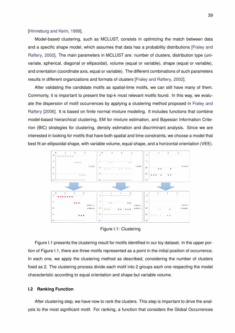
best fit an ellipsoidal shape, with variable volume, equal shape, and a horizontal orientation (VEE).

Figure I.1: Clustering

Figure I.1 presents the clustering result for motifs identified in our toy dataset. In the upper por-

tion of Figure I.1, there are three motifs represented as a point in the initial position of occurrence.

In each one, we apply the clustering method as described, considering the number of clusters

fixed as 2. The clustering process divide each motif into 2 groups each one respecting the model

characteristic according to equal orientation and shape but variable volume.

I.2 Ranking Function

After clustering step, we have now to rank the clusters. This step is important to drive the anal-

ysis to the most significant motif. For ranking, a function that considers the Global Occurrences

40

(GO), Spatial Occurrences (SO), Information Gain (IG) of the motif, and the root mean squared

error (RMSE) for the elements inside clusters with respect to it mean value is applied. Equation

I.1 presents the ranking function proposed.

rankmotif =

∑ RMSEcluster(average)

(IG+1)∗SO2

GO

ncluster(I.1)

The rank sorts motifs by ascending value, put the ones with lowest rank values first. The

objective of ranking function is to prioritize the lowest dispersion with wide spatial range data also

considering the information gain. The GO and SO are parameters returned in motif discovering.

The Information Gain is a classification for motif word according to the variability of data. For each

letter of the alphabet considered in the analysis an associated an unitary incremented vector of

values starting from zero.

For example, in the alphabet considered in the example [a,b,c,d,e] we consider the respective

values [0,1,2,3,4]. In the motif word, the value of Information Gain is computed by making the

absolute difference between each pair of letters combined. Consider motif1 (beeeb) as example.

IG is computed by as IG = |b−e|+ |b−e|+ |b−e|+ |b−b|+ |e−e|+ |e−e|+ |e−b|+ |e−e|+ |e−b|.

Converting the word to a correspondent value vector, we obtain [1,4,4,4,1] then: IG = |1 − 4| +

|1− 4|+ |1− 4|+ |1− 1|+ |4− 4|+ |4− 4|+ |4− 1|+ |4− 4|+ |4− 1| = 12.

41

Bibliography

Agrawal, R., Faloutsos, C., and Swami, A. (1993). Efficient similarity search in sequence

databases. Springer.

Armstrong, T. and Drewniak, E. (2011). Unsupervised discovery of motifs under amplitude scaling

and shifting in time series databases. Lecture Notes in Computer Science (including subseries

Lecture Notes in Artificial Intelligence and Lecture Notes in Bioinformatics), 6871 LNAI:539–

552. 00002.

Berkhin, P. (2006). A survey of clustering data mining techniques. In Grouping multidimensional

data, pages 25–71. Springer.

Box, G. E. P., Jenkins, G. M., and Reinsel, G. C. (2008). Time Series Analysis: Forecasting and

Control. Wiley, Hoboken, N.J, 4 edition edition.

Buhler, J. and Tompa, M. (2002). Finding motifs using random projections. Journal of computa-

tional biology, 9(2):225–242.

Cassisi, C., Aliotta, M., Cannata, A., Montalto, P., Patane, D., Pulvirenti, A., and Spampinato, L.

(2013). Motif discovery on seismic amplitude time series: The case study of mt etna 2011

eruptive activity. Pure and Applied Geophysics, 170(4):529–545.

Castro, N. and Azevedo, P. (2010). Multiresolution motif discovery in time series. In Proceedings

of the 10th SIAM International Conference on Data Mining, SDM 2010, pages 665–676.

Castro, N. and Azevedo, P. (2012). Significant motifs in time series. Statistical Analysis and Data

Mining, 5(1):35–53.

Chan, Y. (2005). Spatial time series. Location, Transport and Land-Use: Modelling Spatial-

Temporal Information, pages 611–711.

Chi, H. and Wang, S. (2013). Finding time series motifs based on cloud model. In Proceedings -

2013 IEEE International Conference on Granular Computing, GrC 2013, pages 70–75.

42

Chi, L. b., Feng, Y., Chi, H., and Huang, Y. (2012). Face image recognition based on time series

motif discovery. In Proceedings - 2012 IEEE International Conference on Granular Computing,

GrC 2012, pages 72–77. 00000.

Chiu, B., Keogh, E., and Lonardi, S. (2003). Probabilistic discovery of time series motifs. In

Proceedings of the ACM SIGKDD International Conference on Knowledge Discovery and Data

Mining, pages 493–498.

Cryer, J. D. and Kellet, N. (1986). Time series analysis, volume 286. Springer.

Daw, C. S., Finney, C. E. A., and Tracy, E. R. (2003). A review of symbolic analysis of experimental

data. Review of Scientific Instruments, 74(2):915–930.

Ding, H., Trajcevski, G., Scheuermann, P., Wang, X., and Keogh, E. (2008). Querying and min-

ing of time series data: experimental comparison of representations and distance measures.

Proceedings of the VLDB Endowment, 1(2):1542–1552.

Esling, P. and Agon, C. (2012). Time-series data mining. ACM Computing Surveys, 45(1).

Ester, M., Kriegel, H.-P., Sander, J., Xu, X., et al. (1996). A density-based algorithm for discovering

clusters in large spatial databases with noise. In Kdd, volume 96, pages 226–231.

Fahad, A., Alshatri, N., Tari, Z., Alamri, A., Khalil, I., Zomaya, A. Y., Foufou, S., and Bouras, A.

(2014). A survey of clustering algorithms for big data: Taxonomy and empirical analysis. IEEE

transactions on emerging topics in computing, 2(3):267–279.

Fan, Y. and Kamath, C. (2015). Identifying and exploiting diurnal motifs in wind generation time se-

ries data. International Journal of Pattern Recognition and Artificial Intelligence, 29(2). 00000.

Ferreira, P., Azevedo, P., Silva, C., and Brito, R. (2006). Mining approximate motifs in time series.

Lecture Notes in Computer Science (including subseries Lecture Notes in Artificial Intelligence

and Lecture Notes in Bioinformatics), 4265 LNAI:89–101.

Fraley, C. and Raftery, A. E. (2002). Model-based clustering, discriminant analysis, and density

estimation. Journal of the American statistical Association, 97(458):611–631.

Fraley, C. and Raftery, A. E. (2006). Mclust version 3: an r package for normal mixture modeling

and model-based clustering. Technical report, DTIC Document.

Fuchs, E., Gruber, T., Nitschke, J., and Sick, B. (2009). On-line motif detection in time series with

SwiftMotif. Pattern Recognition, 42(11):3015–3031.

Hamilton, J. D. (1994). Time series analysis, volume 2. Princeton university press Princeton.

43

Han, J., Cheng, H., Xin, D., and Yan, X. (2007). Frequent pattern mining: Current status and future

directions. Data Mining and Knowledge Discovery, 15(1):55–86. 00786.

Han, J. & Kamber, M. (2006). Data mining: concepts and technique. Morgam Kaufmann, 2.

Hatton, L., Worthington, M. H., and Makin, J. (1986). Seismic data processing: theory and prac-

tice. Technical report, Merlin Profiles Ltd.

Hinneburg, A. and Keim, D. A. (1999). Optimal grid-clustering: Towards breaking the curse of

dimensionality in high-dimensional clustering.

Jiang, T. b., Feng, Y., Zhang, B., Shi, J., and Wang, Y. (2008). Finding motifs of financial data

streams in real time. Lecture Notes in Computer Science (including subseries Lecture Notes in

Artificial Intelligence and Lecture Notes in Bioinformatics), 5370 LNCS:546–555. 00002.

Karypis, G., Han, E.-H., and Kumar, V. (1999). Chameleon: Hierarchical clustering using dynamic

modeling. Computer, 32(8):68–75.

Keogh, E. and Kasetty, S. (2003). On the need for time series data mining benchmarks: a survey

and empirical demonstration. Data Mining and knowledge discovery, 7(4):349–371.

Keogh, E. and Lin, J. (2005). Clustering of time-series subsequences is meaningless: Implications

for previous and future research. Knowledge and Information Systems, 8(2):154–177.

Keogh, E. and Ratanamahatana, C. A. (2005). Exact indexing of dynamic time warping. Knowl-

edge and information systems, 7(3):358–386. 1297.

Keogh, E. J. and Pazzani, M. J. (1998). An enhanced representation of time series which allows

fast and accurate classification, clustering and relevance feedback. In KDD, volume 98, pages

239–243.

Krogh, A. (1998). An introduction to hidden markov models for biological sequences. New Com-

prehensive Biochemistry, 32:45–63.

Lam, H., Pham, N., and Calders, T. (2011). Online discovery of top-k similar motifs in time series

data. In Proceedings of the 11th SIAM International Conference on Data Mining, SDM 2011,

pages 1004–1015.

Lampert, C. H., Blaschko, M. B., and Hofmann, T. (2008). Beyond sliding windows: Object lo-

calization by efficient subwindow search. In Computer Vision and Pattern Recognition, 2008.

CVPR 2008. IEEE Conference on, pages 1–8. IEEE.

44

Last, M., Kandel, A., and Bunke, H. (2004). Data mining in time series databases, volume 57.

World scientific. 00094.

Li, L. and Nallela, S. (2009). Probabilistic discovery of motifs in water level. In 2009 IEEE Interna-

tional Conference on Information Reuse and Integration, IRI 2009, pages 388–393.

Li, Y. and Lin, J. (2010). Approximate variable-length time series motif discovery using gram-

mar inference. In Proceedings of the 10th International Workshop on Multimedia Data Mining,

MDMKDD ’10. 00019.

Li, Z. (2014). Spatiotemporal Pattern Mining: Algorithms and Applications. In Frequent Pattern

Mining, pages 283–306. Springer.

Lin, J., Keogh, E., Lonardi, S., and Chiu, B. (2003). A symbolic representation of time series, with

implications for streaming algorithms. In Proceedings of the 8th ACM SIGMOD workshop on

Research issues in data mining and knowledge discovery, pages 2–11. ACM.

Lin, J., Keogh, E., Wei, L., and Lonardi, S. (2007). Experiencing SAX: A novel symbolic represen-

tation of time series. Data Mining and Knowledge Discovery, 15(2):107–144.

Lin, Y., McCool, M., and Ghorbani, A. (2010). Motif and anomaly discovery of time series based on

subseries join. In Proceedings of the International MultiConference of Engineers and Computer

Scientists 2010, IMECS 2010, pages 481–486.

Liu, Z., Yu, J., Lin, X., Lu, H., and Wang, W. (2005). Locating motifs in time-series data. Lec-

ture Notes in Computer Science (including subseries Lecture Notes in Artificial Intelligence and

Lecture Notes in Bioinformatics), 3518 LNAI:343–353.

Loh, W.-K., Kim, S.-W., and Whang, K.-Y. (2000). Index interpolation: an approach to subse-

quence matching supporting normalization transform in time-series databases. In Proceedings

of the ninth international conference on Information and knowledge management, pages 480–

487. ACM.

Lonardi, J. L. E. K. S. and Patel, P. (2002). Finding motifs in time series. In Proc. of the 2nd

Workshop on Temporal Data Mining, pages 53–68.

Madicar, N., Sivaraks, H., Rodpongpun, S., and Ratanamahatana, C. (2014). An enhanced

parameter-free subsequence time series clustering for high-variability-width data. Advances

in Intelligent Systems and Computing, 287:419–430.

45

McGovern, A., Rosendahl, D., Brown, R., and Droegemeier, K. (2011). Identifying predictive multi-

dimensional time series motifs: An application to severe weather prediction. Data Mining and

Knowledge Discovery, 22(1-2):232–258.

Minnen, D., Isbell, C. L., Essa, I., and Starner, T. (2007). Discovering multivariate motifs using

subsequence density estimation and greedy mixture learning. In Proceedings of the National

Conference on Artificial Intelligence, volume 22, page 615. Menlo Park, CA; Cambridge, MA;

London; AAAI Press; MIT Press; 1999.

Mohammad, Y. and Nishida, T. (2009). Constrained motif discovery in time series. New Generation

Computing, 27(4):319–346.

Mohammad, Y., Ohmoto, Y., and Nishida, T. (2012). G-SteX: Greedy stem extension for free-length

constrained motif discovery. Lecture Notes in Computer Science (including subseries Lecture

Notes in Artificial Intelligence and Lecture Notes in Bioinformatics), 7345 LNAI:417–426. 00000.

Mohammad, Y. b. and Nishida, T. (2014a). Exact discovery of length-range motifs. Lecture Notes

in Computer Science (including subseries Lecture Notes in Artificial Intelligence and Lecture

Notes in Bioinformatics), 8398 LNAI(PART 2):23–32.

Mohammad, Y. b. and Nishida, T. (2014b). Scale invariant multi-length motif discovery. Lecture

Notes in Computer Science (including subseries Lecture Notes in Artificial Intelligence and Lec-

ture Notes in Bioinformatics), 8482 LNAI(PART 2):417–426.

Mueen, A. (2013). Enumeration of time series motifs of all lengths. In Data Mining (ICDM), 2013

IEEE 13th International Conference on, pages 547–556. IEEE.

Mueen, A. (2014). Time series motif discovery: Dimensions and applications. Wiley Interdisci-

plinary Reviews: Data Mining and Knowledge Discovery, 4(2):152–159.

Mueen, A., Keogh, E., Zhu, Q., Cash, S., Westover, M., and Bigdely-Shamlo, N. (2011). A disk-

aware algorithm for time series motif discovery. Data Mining and Knowledge Discovery, 22(1-

2):73–105.

Mueen, A., Keogh, E., Zhu, Q., Cash, S. c., and Westover, B. d. (2009). Exact discovery of

time series motifs. In Society for Industrial and Applied Mathematics - 9th SIAM International

Conference on Data Mining 2009, Proceedings in Applied Mathematics, volume 1, pages 469–

480.

Narang, A. and Bhattacherjee, S. (2010). Parallel exact time series motif discovery. Lecture Notes

in Computer Science (including subseries Lecture Notes in Artificial Intelligence and Lecture

Notes in Bioinformatics), 6272 LNCS(PART 2):304–315.

46

Narang, A. and Bhattcherjee, S. (2011). Real-time approximate range motif discovery & data

redundancy removal algorithm. In ACM International Conference Proceeding Series, pages

485–496. 00000.

Nunthanid, P., Niennattrakul, V., and Ratanamahatana, C. (2011). Discovery of variable length time

series motif. In ECTI-CON 2011 - 8th Electrical Engineering/ Electronics, Computer, Telecom-

munications and Information Technology (ECTI) Association of Thailand - Conference 2011,

pages 472–475.

Nunthanid, P., Niennattrakul, V., and Ratanamahatana, C. (2012). Parameter-free motif discovery

for time series data. In 2012 9th International Conference on Electrical Engineering/Electronics,

Computer, Telecommunications and Information Technology, ECTI-CON 2012.

Patel, P., Keogh, E., Lin, J., and Lonardi, S. (2002). Mining motifs in massive time series

databases. In Data Mining, 2002. ICDM 2003. Proceedings. 2002 IEEE International Con-

ference on, pages 370–377.

Shieh, J. and Keogh, E. (2008). i SAX: indexing and mining terabyte sized time series. In Pro-

ceedings of the 14th ACM SIGKDD international conference on Knowledge discovery and data

mining, pages 623–631. ACM. 00128.

Shumway R. H. & Stoffer, D. S. (2006). Time Series Analysis and Its aplications: with R Examples.

Springer, 2.

Son, N. and Anh, D. (2012). Discovering time series motifs based on multidimensional index and

early abandoning. Lecture Notes in Computer Science (including subseries Lecture Notes in

Artificial Intelligence and Lecture Notes in Bioinformatics), 7653 LNAI(PART 1):72–82.

Son, N. T. and Anh, D. T. (2016). Discovery of time series k-motifs based on multidimensional

index. Knowledge and Information Systems, 46(1):59–86.

Staden, R. (1989). Methods for discovering novel motifs in nucleic acid sequences. Computer

applications in the biosciences: CABIOS, 5(4):293–298.

Tanaka, Y., Iwamoto, K., and Uehara, K. (2005). Discovery of time-series motif from multi-

dimensional data based on mdl principle. Machine Learning, 58(2-3):269–300.

Tanaka, Y. and Uehara, K. (2003). Discover motifs in multi-dimensional time-series using the

principal component analysis and the mdl principle. In Lecture Notes in Artificial Intelligence

(Subseries of Lecture Notes in Computer Science), volume 2734, pages 252–265.

47

Tang, H. and Liao, S. (2008). Discovering original motifs with different lengths from time series.

Knowledge-Based Systems, 21(7):666–671.

Truong, C. and Anh, D. (2013). An efficient method for discovering motifs in large time series.

Lecture Notes in Computer Science (including subseries Lecture Notes in Artificial Intelligence

and Lecture Notes in Bioinformatics), 7802 LNAI(PART 1):135–145.

Truong, C. and Anh, D. (2015). A fast method for motif discovery in large time series database

under dynamic time warping. Advances in Intelligent Systems and Computing, 326:155–167.

Tsai, C.-W., Lai, C.-F., Chao, H.-C., and Vasilakos, A. V. (2015). Big data analytics: a survey.

Journal of Big Data, 2(1):1–32.

Vahdatpour, A., Amini, N., and Sarrafzadeh, M. (2009). Toward unsupervised activity discovery

using multi-dimensional motif detection in time series. In IJCAI International Joint Conference

on Artificial Intelligence, pages 1261–1266. 00053.

Van Hoan, M. and Exbrayat, M. (2013). Time series symbolization and search for frequent pat-

terns. In ACM International Conference Proceeding Series, pages 108–117. 00000.

Wang, L., Chng, E., and Li, H. b. c. (2010). A tree-construction search approach for multivariate

time series motifs discovery. Pattern Recognition Letters, 31(9):869–875.

Wei, W. W.-S. (1994). Time series analysis. Addison-Wesley publ Reading.

Wilson, W., Feyereisl, J., and Aickelin, U. (2007). Detecting motifs in system call sequences.

Lecture Notes in Computer Science (including subseries Lecture Notes in Artificial Intelligence

and Lecture Notes in Bioinformatics), 4867 LNCS:157–172. 00000.

Yang, J., Wang, W., and Philip, S. Y. (2004). Mining surprising periodic patterns. Data Mining and

Knowledge Discovery, 9(2):189–216.

Yankov, D., Keogh, E., Medina, J., Chiu, B., and Zordan, V. (2007). Detecting time series mo-

tifs under uniform scaling. In Proceedings of the ACM SIGKDD International Conference on

Knowledge Discovery and Data Mining, pages 844–853.

Yilmaz, O. (2001). Seismic data analysis, volume 1. Society of exploration geophysicists Tulsa.

Zhou, H.-W. (2014). Practical seismic data analysis. Cambridge University Press.