Abstract

An efficient data structure for representing the set of all distinct planar embeddings of a biconnected graph is given (This data stucture is based on PQ- trees [3]). Algorithms are presented for constructing the data structure, for extracting from it all embeddings (or the number of distinct embeddings), and for updating it to incorporate new constraints. The constraints considered here further restrict the clockwise order of edges about vertices. The data structure also suggests a new approach to proving the correctness of planarity testing and embedding algorithms based on PQ-trees (see [3], [4], and [21]).

1. Introduction

Planar embeddings of graphs are used in a variety of applications. They range from faster algorithms for the planar special case of general graph problems (see e.g. [2,7,14,17]) to checking isomorphism of chemical structures (an application of planar graph isomorphism, see [9,11]) to VLSI design (see, e.g. [1,6,8,16,20]). This paper presents a data structure based on PQ-trees (see [3]), which represents all possible embeddings of a planar graph in linear space. The data structure can be constructed in linear time using an algorithm similar to that of [3]. Efficient solu- tions to the following problems are given:

(a) producing one embedding of the graph,

(b) producing all embeddings of the graph,

(c) verifying that a given embedding is in fact an embedding,

(d) producing one (all) embeddings of the graph subject to addit,ional constraints on the order of edges about a given set of vertices.

The time required for all of these problems is linear in the size of the input (or out- put in the case of producing all embeddings). The solution to an online version of problem (d) is also discussed. The time bound in this case is almost linear.

The author was recently made aware that solutions to problems (a) and (b) based on PQ-trees have appeared in [4] (problem (a) can also be solved in linear time by an algorithm based on the planarity testing algorithm of [lo]).

The approach used in this paper differs in several ways from that of 141. First, PQ-trees are used here to represent the set of all possible embeddings as well as in the initial planarity t,esting/embedding phase. This allows consideration of the verification and update problems (c) and (d). Furthermore this paper relates the structure of PQ-trees to a partitioning method developed by MacLane [15] to determine the number of distinct planar embeddings of a graph. In particular, we show that in the PQ-tree representation used during planarity testing, P-nodes represent branch graphs and Q-nodes represent triply connected components. Finally, the basic embedding algorithm presented here is more elegant than that of [4] in that it does not require the use of "direction indicators" to keep track of the left to right orientation of Q-nodes.

A graph G is a set of edges, each edge connecting two (not necessarily dis- tinct) vertices in V ( G ) . Multiple edges and loops are permitted. Each edge in G is said to be incident to the two vertices of V(G) that it connects.

The graphs that are inputs to our algorithms are assumed to be biconnected (this rules out loops). It is well known that a graph is planar iff its biconnected components are planar and that an embedding for a graph can be obtained from embeddings of the biconnected components. Section 8 discusses the extension of the verification result (problem (c) above) to graphs that are not biconnected.

Unfortunately the remaining results appear to be difficult to extend.

Definition 1.1. A graph G is planar if its edges can be drawn on the plane without crossings. In reference to such a drawing, a face is a connected region of what remains of the plane when all the edges of 0 are removed. A face boundary is a subset of G that forms the boundary of a face. An embedding of a biconnected graph G is a set of cycles in G that are face boundaries.

Another way to define an embedding is by giving a clockwise ordering of the edges incident to each vertex in a drawing. This latter definition will be used in the algorithms presented here. However, Definition 1.1 is needed to determine whether two embeddings are distinct. In particular, two clockwise orderings represent the same embedding if (a) any list of edges is rotated (the list begins a t a different edge) or (b) all lists of edges are reversed (if the drawing is reflected, the same embedding results).

Definition 1.2. A primitive constraint on the embedding of a graph is a triple ( e , f , v ) , where e and f are edges incident to the vertex v . It means that only those embeddings in which e and f appear consecutively around v are to be allowed. A compound constraint is a set of primitive constraints {(e ,, f ,,v,), . - . , ( e k , fk ,vk)} such that for each i , e precedes f z in a clockwise ord- ering of edges about vz .

Note that for a compound constraint all primitive constraints must be satisfied simultaneously with the same clockwise orientation. For example, con- sider the embedding pictured in Figure 1. It satisfies the primitive constraints a , b ,1) and (d , e ,3) but not the compound constraint {(a,b , l ) , (d ,e ,3)}. I11 fact, no embedding of the graph in Figure 1 satisfies this particular compound constraint.

Definition 1.3. The off-line embedding constraint problem (0FE;C) is the follow- ing: Given a graph G and a list of compound constraints L , produce an embedding of G that satisfies all the constraints in L or conclude that no such embedding is possible. Two variations on OFEC are solved by the same technique. Either ask for all embeddings satisfying the constraints (all-OFEC) or the number of distinct embeddings satisfying the constraints (#-OFEC).

The problems of producing an embedding of a planar graph and verifying an embedding (problems (a) and (c) above) are both special cases of OFEC. For the verification problem the embedding may be represented either as a set of face boundaries or as a set of clockwise edge lists about each vertex. Consider, for example, the situation where an embedding is represented as a set of face boun- daries. It is a simple matter to translate the set of edges forming a face boundary (given in arbitrary order) to a list of the form eo, ..., ek_,, where e and e,,+iimdi

are incident to the same vertex v . For each such list, that is, for each face boun- dary, we introduce the compound constraint {(eo,e .,v0), ( e k - l , e o 7 ~ k - l ) b

The above discussion also implies that various kinds of "partial embeddings" can be verified using the OFEC problem. For example, we may want to ensure that certain cycles of the graph appear as face boundaries in an embedding (this is of particular interest for the rnultiroiriniodity flow problems discussed in [17]).

Definition 1.4. The on-line embedding constraint problem (ONEC) is the on-line version of OFEC. From a graph G a data structure encoding the set of all possible embeddings of G is computed. Constraints are added on-line, one primitive con- straint at a time. After each primitive constraint is added, the alg~ri t~hrn either updates the data structure to reflect the new contraint or reports that the new con- straint is inconsistent with t,he current set of possible embeddings. The \ ariations all-ONEC and #-ONEC are analogous to all-OFEC and #-OFEC.

The ONEC problem comes from the following situation. Suppose one is try- ing to produce a layout for a VLSI circuit made up of smaller components for which layouts already exist. Let G be the set of interconnections among the com- ponents. The existing layouts impose constraints on the relative order of the inter- connections within the same component. One way to tackle this problem is to list the constraints in order of importance, updating the set of possible embeddings until only a small number remains. Each of the remaining embeddings can then be evaluated with respect to the cost of redesigning existing components and other considerations.

We solve both the OFEC and the ONEC problems in two stages. The first stage constructs a PQ-tree based data structure EMBEDDINGS(G) from a bicon- nected planar graph G . In the second stage EMBEDDINGS(G) is updated to incorporate all constraints. The chief difference between our solutions to OFEC and ONEC is that an off-line approach permits certain consistency tests (having to do with the relative clockwise orientation of one part of the graph wrt another) to be deferred until all constraints have been processed.

The main results are as follows. Let m = \ G 1, i.e. the number of edges in the graph. Note that because of multiple edges, m may not be 0() v (G ' )~) (m is o(\V(~)l) in a planar graph with no multiple edges). Then EMBEDDINGS(G) can be constructed in 0 ( m ) time. Generating one embedding from EMBEDDINGS(G) also takes 0 ( m ) time. T o generate all distinct embeddings requires time O(md), where d is the number of embeddings generated; note that the size of the output is O(md) in this case.

Let p be the number of primitive constraints. Then the problems OFEC and #-OFEC can be solved in time O(m + p ) , whereas all-OFEC takes time 0 ( m d + p ) (d is the number of embeddings that satisfy the constraints). ONEC takes total time O(m + pa(p ,c +log</)), where c is the number of compound constraints and d is the number of embeddings of the original graph. The number of distinct embeddings can be maintained and updated with no increase in asymptotic cost.

The results are presented in the following order. Section 2 introduces PQ- trees and describes the modifications needed to maintain EMBEDDI.;VGS(G). In

Section 3 the problems of generating all embeddings and of keeping track of the number of embeddings are discussed wrt EMBEDDINGS(G). Section 4 talks about how EMBEDDINGS(G) is updated to reflect constraints as defined by Definition 1.2. Both the off-line and the on-line version of the update algorithm are discussed. Section 5 gives the algorithm for generating EMBEDDINGS(G) from a biconnected planar graph G and proposes an alternate view of the algo- rithm suggested by the work of MacLane [15] (the same interpretation can also be applied to the planarity algorithms of [3,4,13]). This alternate view can be used as the basis for a rigorous correctness proof of the algorithm for generating EMBEDDINGS(G) (as well as for the algorithms in [3,4]). A sketch of this proof is given in Section 6. Section 7 discusses open problems with special emphasis on graphs that are not biconnected.

2. T h e P Q - t r e e D a t a S t r u c t u r e

The implementation of EA4BEDDINGS(C\ the data structure used the algo- rithms described in Sections 3 and 4, is based on PQ-trees [3]. The set of possible clockwise orderings of edges incident to each vertex is represented by a forest of PQ-trees. Trees of the forest are related to each other in ways that reflect the degrees of freedom of the embeddings of the graph (Sections 5 and 6 deal with this point in more detail). We show here that the required relationships are easy to irnplemen t within the framework of the PQ-tree algorithms discussed in [3,2 11.

First, we observe that G can be converted into a directed graph in such a way that the incoming edges to any vertex can be separated from the outgoing edges in a clockwise ordering.

Lemma 2.1. 1131 In a biconnected graph G with n vertices. the vertices can be numbered in such a way that vertex 1 is adjacent to vertex n and every other ver- tex has at least one neighbor with a lower number and one neighbor with a higher number.

Definition 2.1. The numbering described in Lemma 2.1 is called an st- numbering.

An st-numbering for a biconnected graph can be found in linear time [5]. Henceforth, we assume that the vertices of any biconnected graph G are st- numbered and use x (: V ( G ) and its st-number interchangeably. There may be several st-numberings of any graph, but the essential properties used in this discus- sion hold for any st-numbering.

L e m m a 2.2. Let G be a biconnected planar graph with vertices numbered using an st-numbering, and let a ( G ) be any embedding of G . Then a representation of a ( G ) as a set of clockwise lists of edges about each vertex always has edges to higher (from lower) numbered vertices appearing consecutively in every list.

Proof . Suppose not. Then there exists a vertex v whose clockwise list, after a number of edges are deleted from G (deletion of edges does not affect an embed- ding), is e l , f .,en, f 2, where the e are edges to lower numbered vertices and the f f to higher numbered vertices. Let u be the other endpoint of e and w the other endpoint of f . Then by a series of edge contractions (contraction does not affect the embedding or the clockwise order of edges around v ) ul and u2 can be identified with vertex 1, while wl and w2 are identified with vertex n . In the sub- graph G consisting only of the edges incident to v , vertices 1 and n have degree 2. Eliminating them (which does not affect the embedding) leaves an embedding of two loops, e and f (composed of e 's and f 's, respectively) in a clockwise order of e , f , e , f about v . This is obviously impossible without edge crossings.

Essentially the same Lemma is proved in [13] using a different approach.

Suppose vertices are numbered using an st-numbering and a drawing is arranged so that lower numbered vertices appear closer to the top than higher numbered vertices. Then the corresponding embedding can be represented by specifying the left to right ordering of the edges from lower numbered vertices to each vertex and the left to right ordering of edges to higher numbered vert,ices from each vertex (we now regard all edges as being directed from lower numbers to higher numbers).

Let I n ( i ) be the left to right ordering of edges from vertices whose number is < i to vertex number i, and Out ( i) be the left to right ordering of edges from ver- tex number i to vertices whose number is > i. Then for the picture in Figure 2, the lists are

In(1) = 0, Out(1) = a b c In (2) = a , Out(2) = j g d e In (3) = d , Out (3) = i h In(4) = h e , Out (4) = J In(5) = j g i j b c , Out (5) = 0

A clockwise ordering around vertex i is given as I n ( i ) followed by Out(i) in reverse order. Two sets of left to right lists specify the same embedding if all the lists in one set are the reverse of all the lists in the other.

EMBEDDINGS(G) is a forest of PQ-trees. For each v <: V ( G ) , there is a tree representing In ( v ) and another tree representing Out ( v ) .

Definition 2.2. A PQ-tree (see [3]) specifies a set of admissible permutations on a ground set S, in this case the set of edges incident to a particular vertex. The leaves of a PQ-tree represent elements of S. In addition, there are two types of interior nodes. A P-node specifies that its children may appear in any order, but all leaf descendants of the P-node must appear consecutively. A Q-node specifies that its children must appear in the order they are listed or the reverse of that order.

In our notation for PQ-trees, angle brackets <> enclose the children of a P- node, while square brackets are used to enclose the children of a Q-node. For example, [<a b c > d e l denotes a PQ-tree whose root is a Q-node with three children: a P-node and the leaves d and e. The P-node has three children: the leaves a , b, and c . Among the admissible permutations of the five leaves are abcde, edabc (reverse children of Q-node), and bacde (permute children of the P- node). Not admissible are the permutations dabce (violates constraint imposed by Q-node) and abdce (violates P-node constraint).

Nodes of one tree in EMBEDDINGS(G) may be related to nodes of another tree. In particular, every child of a P-node in the forest has a unique mate. If the children of a P-node are permuted in any way, their mates must be permuted in the same way. Furthermore all interior nodes are grouped into equivalence classes wrt an equivalence relation = . If X = Y, where X and Y are both P-nodes, then the children of X are mates of the children of Y. X and Y always have the same

number of children in this case. If X and Y are Q-nodes, then a reversal of the order of X 's children implies that the order of the children of Y must be reversed as well. An equivalence class wrt = either contains exactly two P-nodes with the same number of children or an arbitrary number of Q-nodes. A P-node and a Q- node never appear in the same class.

Our notation for PQ-trees uses subscripts to denote equivalence classes wrt == . The closing angle or square bracket for each interior node has a subscript identifying its equivalence class.

For example, if G is the graph depicted in Figure 2, then EMBEDDINGS(G) is given by the PQ-trees below.

In(1): 0; Out (1): <a b c > A

In(2): a ; Out(2): <f g [ d e ] B > c In(3): d ; Out(3): [ i hIB In(-4): [h elB; Out(4): J'

In(5): <<f g [i j]B>c b c > ^ ; Out(5): 0 Note that the permutation of a , b , and c around vertex 1 influences the permuta- tion of {/ , g .h ,j}, b , and c around vertex 5. The equivalence class denoted by the subscript A keeps track of this relationship. It contains two P-nodes, each of which has 3 children and the corresponding children are mates of each other. Note also that {d ,e ,h , i , l} is a triply connected component of the graph, and that the rever- sal of the order of d and e around vertex 2 forces all other parts of the component to be reversed. The Q-nodes with subscript B represent this triply connected com- ponent.

In the example just described, there are several Q-nodes which have only two children. The formulation of [3] disallows such Q-nodes, replacing them by equivalent P-nodes. From our point of view, however, it is important to allow Q- nodes with two children, and to distinguish between these and P-nodes with two children. As we shall see later, a Q-node with two children represents a triply con- nected component, whereas a P-node with two children represents two disjoint paths in the graph.

PQ-trees are characterized by the operation Reduce(T,S1), where T is a PQ- tree defined on S and 5" C S. Reduce( T ,S1) transforms T in such a way that the elements of S t are forced to be consecutive, or indicates that such a transformation is impossible. We refer to [3] or [21] for a detailed discussion of Reduce and its linear time implementation. The following description suffices for this discussion.

Definition 2.3. [3] The nodes of a PQ-tree T may be classified as follows in rela- tion to the operation Reduce( T , S t ) . A node is said to be full if it is a leaf in S' or if all of its leaf descendants are full. A node is empty if it is a leaf not in 5" or if all of its leaf descendants are empty. A node is partial if some of its leaf descendants are full and others are empty. The lowest common ancestor of all full nodes is called the subroot, also denoted by ROOT ( T ,S ').

The algorithm for Reduce in [3] relies on a set of local transformations called templates which may be applied in a bottom up fashion. Young [21] gives a top- down approach that is slightly more elegant, but in principle the same set of tem- plates is used. The modifications dealing with mates and equivalence classes, as described below, apply to either implementation. A complete list of the relevant templates is given in Figure 3. Note that some templates only apply if the node in question is the subroot. In every case, empty children are denoted by e and full children by f

Dealing with mates of P-node children is straightforward. Any transforma- tion that puts further constraints on the order of the children of a P-node must be applied to their mates as well. One example suffices to illustrate the principle. Consider template (P3) of the Reduce algorithm (see Figure 3), and let X be the P-node labelled A , Y the P-node labelled B , and Z the Q-node labelled C . When the template is applied some of the children of X become children of t h e new P- node Y. Then both X and Y become children of the new Q-node Z . Suppose X' = X (X' is the unique element of A - {X}). To take care of the children of X', a new P-node Y ' = Y is created. The mates of the children of I' become chil- dren of Y'. Then, a new Q-node 2' becomes the parent of X' and Y ' . To ensure that the constraints on mates are faithfully preserved, 2' = 2. Note that all operations involving mates can be done within the same time bound a5 the opera- tions they mimic. For any P-node X, we need to be able to access the unique X' = X and mate( W) for any W that is a child of X. The maintainance of the necessary pointers is straightforward.

Maintaining equivalence classes of Q-nodes requires more care. Consider the template (Q2) (Figure 3) and let X be the Q-node labelled A , Y the Q-node labelled B (template (Q3) is similar). It is clear that the equivalence classes A and B must be combined in this case. The problem is that the order of the children of Y might have to be reversed when this template is applied. This would mean the that the order of the children for all Q-nodes in the same equivalence class as Y would have to be reversed.

Instead of performing these reversals, the algorithms described in Section 4 maintain a separate data structure to keep track of which Q-nodes need to be reversed relative to other Q-nodes. The operation Merge(X, Y,reverse) updates this structure by merging the equivalence classes for X and Y and recording whether X's orientation is reversed relative to Y's (reverse is true if so). Since the implementation of the auxiliary data structure depends on whether we are solving an off-line or an on-line problem, details are deferred until Section 4.

A more immediate concern is the detection of the relative orientation of two Q-nodes. In the implementation of the Reduce operation described in [3] or [21], only the end children of Q-nodes have correct parent pointers. Furthermore, the list of children for a Q-node is doubly linked, but the links are not guaranteed to point in the same direction (see Figure 4). These lapses are essential for the linear time bound; without them, the updates required to implement a transformation

like template (Q2) would be too costly.

Instead of correctly updating all links and parent pointers, we keep old parent point,ers intact (even if they point to nodes that are no longer part of any tree) and ensure that the left/right sibling pointers among the children of a Q-node are correct relative to t h e p a r e n t po in ter . That is, once any node becomes the child of a Q-node, its parent pointer never changes unless it becomes an end child of another Q-node. Sibling pointers are adjusted only if the parent pointer changes. For an end child of a Q-node it is easy to detect whether it is the left or right end child.

Figure 4 illustrates what happens after a series of applications of template (Q2). In Figure 4(b) note that only c is made aware of the new parent. Accord- ingly, only c 's leftlright sibling pointers are revised to be consistent with the orien- tation of the new parent. The discontinuity in sibling pointers between b and e or between Z and c indicates that Y was reversed in relation to X. If, a t some later t,ime, Z and X are involved in a (Q2) template as illustrated in Figure 4(c), then the orientation of Z relative to X or Y is determined. The discontinuity between d and f indicates that Z is reversed realtive to Y. However, since h and c 's sibling point,ers are consistent, we know that Z has the same orientation as X.

3. Algorithms for Enumeration Problems

Generating a single embedding of a planar graph G is relatively simple when EMBEDDINGS(G) is given. This holds too when the set of embeddings is subject to further constraints as described in the next section. We turn our attention now to the problems of giving the number of embeddings represented by EMBEDDINGS(G) and generating all embeddings represented by EA-/BEDDINGS ( G).

In general, if a P-node X and the unique X ' = X each have k children, there are k ! different ways to permute the children of X and X'. Similarly, there are two possibilities for each equivalence class of Q-nodes: list all the children of each Q-node in the order of appearance or reverse the order for every Q-node in the class.

A naive and almost correct approach for computing the number of embed- dings from ElVfBEDDI"VGS(G) is to count the number of children for each equivalence class of P-nodes and the number of equivalence classes of Q-nodes, computing the number of embeddings as follows. Suppose there are p classes of P-nodes having k., ..., k children, respectively, and q equivalence classes of Q-

P nodes. Then the number of embeddings should be k.\- - . - -kp!-2q. That is, take into account all possible permutations of the children of each P-node and reversal of the children of each Q-node.

This approach ends up counting some embeddings twice. Consider the simple graph G shown in Figure 5. Here, EMBEDDINGS(G) is

In (1): 0; Out (1): <a b c > A

In(2): <a b c > A ; Out ( 2 ) : 0 The naive formula suggests that there are 6 embeddings. But in fact there is only one, the one whose face boundaries are ab, be, and ac .

The overcounting comes from two sources. First, if any clockwise edge list is simply rotated, the resulting embedding remains the same. Second, a reversal of all clockwise edge lists keeps the embedding the same. The problem is solved by designating one equivalence class as the fixed class, effectively using it as a refer- ence point for the whole embedding. If the fixed class contains two P-nodes each having k children (k > 2), the children have only (k - l)!/2 possible rearragements (this is half the number of circular permutations of k items and thus corrects for both rotations and reversals). In the above example, where k = 3, only one embedding results. A fixed class containing Q-nodes is simply not counted (here, reversal is the only possible rearrangement, and it leads to the same embedding).

The algorithm for constructing EMBEDDINGS(G) (Section 5) chooses a fixed class. Unless G is a simple cycle the fixed class never contains P-nodes with just 2 children.

For example, the number of embeddings for the graph in Figure 2 is 3! -2 - (3 - l)! = 12. We note here that the choice of the fixed class is not arbitrary (choosing class B as the fixed class rather than class A would not give the same

result). The issue of which class must be chosen as the fixed class is deferred until Section 5. Full justification for the choice of the fixed class can be found in Section 6.

It is easy to see how the number of embeddings can be updated when addi- tional constraints affect the structure of EMBEDDINGS(G). As described in the next section, such updates are accomplished by a series of Reduce operations on the appropriate trees in the forest. When two equivalence classes of Q-nodes are merged, the count is divided by 2. The appropriate adjustments for templates that affect the number of children of P-nodes are easy to calculate.

The only sticky issue with respect to updates is what happens to the fixed class when it is altered or disappears entirely. When a fixed class of Q-nodes is merged with another class, the combined class becomes the new fixed class. If the fixed class contains two P-nodes, we maintain the following invariants.

(i) The P-nodes have more than 2 children (except when G is a simple cycle).

(ii) The P-nodes are always roots of whatever tree they appear in.

The algorithm in Section 5 ensures that both invariants are true initially for EMBEDDINGS(C). For subsequent updates the only relevant templates are (P2), (P4), and (P6), since these are the only templates that can apply when a P-node is the root of the tree. We must deal with the possibility that p < 2 (see Figure 3) for each of these templates. Since (P2) requires special handling during the update phase, we defer further discussion of it until the next section. For (P4) and (P6), when the original fixed class is A and p < 2, the new fixed class is B. This is clearly the correct choice when p = 0 and class A disappears entirely. When p = I , the class A still survives but it must not be counted when distinct embed- dings are enumerated. A straightforward analysis of the effect of (P4) or (P6) on circular permutations of the original s - r + 2 (P4) or t - s + 3 (P6) children verifies that this is the correct approach. In either case, the new fixed class is a class of Q- nodes, not subject to the invariants.

In order for EMBEDDINGS(G) to be used for the purpose of enumerating embeddings, we must include in the data structure a designation of the fixed class and a list of "active" classes L(G) (classes that are to used in the count; the fixed class is not in L ( G)). Suppose L ( G ) contains p classes of P-nodes having kl, ...

7 %

children, respectively, and q classes of Q-nodes. Then the number of distinct embeddings is k - -k ! .2q - - ( h - I)! if the fixed class contains P-nodes with h

P children and k ! . - - - k ! - 2 if the fixed class contains Q-nodes.

Assuming constant time per arithmetic operation, this can be computed in time 0 ( r ) , where r is the number of equivalence classes. Note that r is 0 ( m ) because the it is bounded by the number of interior nodes in the forest and thus by the number of leaves. In practice there is no need to compute the number of embeddings unless it is of reasonable size.

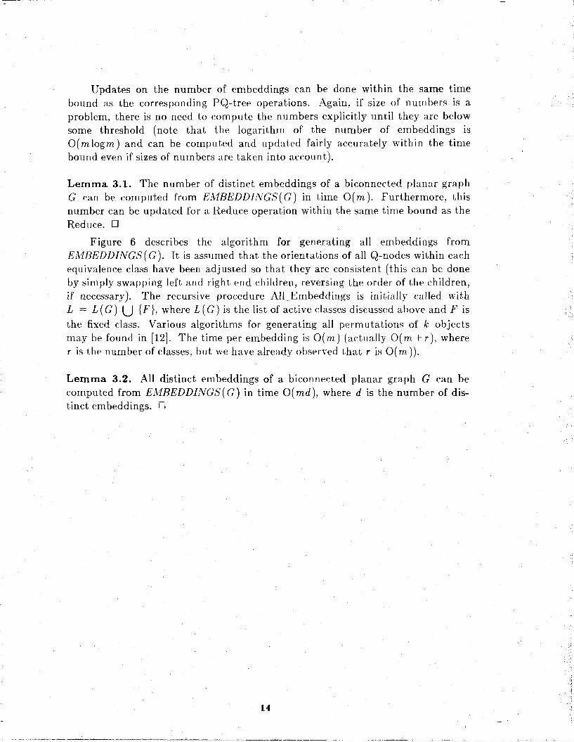
Updates on the number of embeddings can be done within the same time bound as the corresponding PQ-tree operations. Again, if size of numbers is a problem, there is no need to compute the numbers explicitly until they are below some threshold (note that the logarithm of the number of embeddings is O(m1ogm) and can be computed and updated fairly accurately within the time bound even if sizes of numbers are taken into account).

Lemma 3.1. The number of distinct embeddings of a biconnected planar graph G can be computed from EMBEDDINGS(G) in time 0 ( m ) . Furthermore, this number can be updated for a Reduce operation within the same time bound as the Reduce. 0

Figure 6 describes the algorithm for generating all embeddings from EMBEDDINGS(G). It is assumed that the orientations of all Q-nodes within each equivalence class have been adjusted so that they are consistent (this can be done by simply swapping left and right end children, reversing the order of the children, if necessary). The recursive procedure All-Embeddings is initially called with L = L ( G ) 1) {F }, where L (G ) is the list of active classes discussed above and F is the fixed class. Various algorithms for generating all permutations of k objects may be found in [l2]. The time per embedding is 0 ( m ) (actually O(m + r ) , where r is the number of classes, but we have already observed that r is O(m )).

Lemma 3.2. All distinct embeddings of a biconnected planar graph G can be computed from EMBEDDINGS(G) in time O(md), where d is the number of dis- tinct embeddings. D

4. Algorithms for Constraint Problems This section discusses how EMBEDDINGS(G) is used to solve the problems

OFEC and ONEC. Combined with the ideas of the previous section, this leads to algorithms for the all-OFEC, all-ONEC, #-OFEC, and #-ONEC problems as well. The algorithm for generating EMBEDDINGS(G) from G is discussed in Section 5.

Both the off-line and the on-line algorithms given here incorporate additional constraints by updating EMBEDDINGS(G). They differ only in their method for updating the equivalence relation among Q-nodes. The off-line algorithm con- structs a graph of all the dependencies among orientations of Q-nodes. This graph is checked for consistency and the equivalence classes are consolidated only after all constraints have been processed. The on-line algorithm, on the other hand, updates the equivalence relation each time a Merge(X, Y,reverse) (see Section 2) takes place. If X and Y are already in the same equivalence class, the on-line algo- rithm also needs to check that the relative orientation given by reverse is con- sistent with the one that is already known (based on previous Merge's). This is accomplished using the compressed trees technique described in [l8].

We begin by giving the details that are common to both algorithms. Suppose ( e , f , u ) is an arbitrary primitive constraint. If e and f both lead from lower num- bered vertices to u , or both lead from v to higher numbered vertices, then the operation Reduce( T ,{e , f }), where T is the PQ-tree representing In ( v ) , resper- tively Out(v), transforms EMBEDDINGS(G) so that all embeddings are subject to the primitive constraint.

The difficulty arises when e is directed into v and f is directed out of u , or vice versa. To take care of this problem, each PQ-tree representing an In or Out list is modified. A new Q-node is added as the root, so that the tree now looks like

[ *left * original tree *right *\. . *left* and *right* are new leaves that mark the left and right boundaries of each list. All of the new Q-nodes are put into the same equivalence class A , separate from all other equivalence classes. A is ignored when the number of embeddings is counted or when all ernbeddings are generated (in particular, it is not included on the list L ( G ) described in the previous section). However, the new class may even- tually be merged with another class and a t that point the other class is still included in L (G).

The primitive constraint described above is handled by doing two transforma- tions, Reduce( T(In(v)),{e , *right*}) and Reduce(T(0ut (u)),{f , *right*}). Note that if all constraints are primitive there is no need for both left and right markers. The relative orientation of two primitive constraints does not matter in that case.

Special treatment must be given to vertices 1 and n (and any other vertex that has only one tree -- see Section 5 for other cases). We need to somehow represent Out (1) and I n ( n ) as circular lists, whereas PQ-trees are designed for linear lists. Consider the tree representing Out(1) for the graph in Figure 5 , <a b c >., and suppose the three primitive constraints ( a , b , l), (6 , c ,I), and

( c ,a ,1) are presented to the update algorithm. After the first two constraints, the . tree for Out(1) is [a b c I n , where B is a new equivalence class introduced by the

constraints. Now Reduce(T,{c ,a}), where T is the tree for Out(l) , is impossible, even though the constraint can clearly be satisfied.

We deal with the situation by using the *left * and *right * boundary markers in a different way. If Reduce(T,{e, f }) fails, where T is the unique tree for some vertex (typically vertex 1 or n ) , then we try again with Reduce( T ,{e , *right *}) fol- lowed by Reduce( T ,{ *left*, f \}. In the example discussed above, the final result is [*left* a b c *right*\^.

Abandoning an unsuccessful Reduce in order to try a different one presents some implementation problems for the algorithm described in 131. Some templates that were applied successfully might have to be "undone." However, the implemen- tation in [21] is able to test for an irreducible configuration without altering the tree in any way.

For a compound constraint of the form {(e ,, f , , v ) , - - , (ek, f ,vk)}, where k > 1, we need to ensure that the orientation of all the primitive constraints is consistent (either all clockwise or all counter-clockwise). This is done by introduc- ing a new equivalence class of Q-nodes for the constraint. The Reduce operation is modified slightly so that the subroot after the transformation is always a Q-node. Note that P2 is the only template for which this is not the case. The obvious modification is given below (note that there can be a t most two full children of the subroot when Reduce is wrt a primitive constraint).

ce1 ' " e p f I f 2 > A 4 < e l " ' e p [ f 1 f 2 ] B > A If A is the fixed class and p = 1, the new fixed class is B (see the previous section for a futher discussion of fixed classes).

Every primitive constraint generates a Q-node and the Q-nodes for e 1 , f ̂ ,v , ) , - - . , (ek,fk,vk), are all put into the same equivalence class. This ensures that the relative orientation will always be consistent. Figure 7 gives full details of the algorithm that processes one compound constraint.

We now discuss the two approaches to maintaining the equivalence relation among Q-nodes. The off-line algorithm stores == in the form of an undirected labelled graph G . The vertices of GQ are the Q-nodes. Each time a

~ e r ~ e ( ~ , ~ , r e v e r s e ) is done, an edge between X and Y is added to Gn. The label on that edge is either a 0 or a 1, depending on whether reverse is false or true.

When all constraints have been processed, the procedure Collapse performs two operations on G First, it checks to make sure that no cycles of odd length Q - exist (where the length of an edge is given by its label). A cycle of odd length implies that there is an inconsistency in the orientations of the Q-nodes. Then Collapse replaces each connected component of GQ with one representative Q-node for that component. Note that each component of GQ corresponds to an equivalence class. Ultimately every Q-node X ends up with a pointer R E P ( X ) , the representative of its equivalence class, and a boolean indicator R E V ( X ) to indicate

whether X's orientation has to be reversed relative tJo R E P ( X ) . Both of the opera- tions performed by Collapse can be performed in time linear in the size of GQ using depth first search. The Reduce transformations used in processing the con- straints take time O(m + p).

Theorem 4.1. The OFEC problem can be solved in time O(m + p ) , where m is the size of the input graph and p is the number of primitive constraints. 0

Corollary 4.1. An embedding of a planar graph can be verified in linear time.

Corollary 4 .2 . The all-OFEC problem can be solved in time 0 ( m d + p) , where d is the number of embeddings generated.

Corollary 4.3. The #-OFEC problem can be solved in time O(m + p). [I

For the on-line algorithm, we use the set merging techniques of [18]. Every Q- node appears in a forest of trees, each tree representing one equivalence class. The pointer PAR(X) points to X's parent in the forest, or to X itself if X is a root. REV(X) tells whether X's orientation must be reversed relative to P A R (X). The algorithm for Merge is given in Figure 8.

The time bound, based on Tarjan's analysis [l8], is O(m + pa (p , r ) ) , where r is the total number of Q-nodes. From the algorithm described in Section 5 it is apparent that EMBEDDINGS(G) can be set up in such a way that each equivalence class of Q-nodes has a unique representative known to all nodes of the class. Furthermore, the new Q-nodes generated by primitive constraints each belong to a particular compound constraint and we can designate a unique representative for all Q-nodes generated by each compound constraint. It is clear that we need only include the unique representative of each class in our count for r . Thus r = the number of equivalence classes of Q-nodes in the initial structure of EMBEDDINGS(G) plus the number of compound constraints. The former is O(logd), where d is the number of embeddings of the original graph (by the analysis of the previous section every distinct equivalence class of Q-nodes except for the fixed class doubles the number of embeddings).

It is important to note that the time bound from 1181 is amortized, and assumes in this case a sequence of f l ( c +logd) Merge operations, or, putting it another way, it assumes the number of equivalence classes of Q-nodes is reduced to a constant. This is a realistic assumption in most settings (particularly the appli- cation described in Section I) , since it is certainly satisfied when the additional constraints reduce the number of embeddings to a constant (the number of Q-node equivalence classes is then reduced to a constant as well).

Theorem 4.2. The ONEC problem can be solved in time O(m + p a ( p ,c + logd)), where c is the number of constraints and d is the number of embeddings of the original graph.

Corollary 4.4. The #-ONRC problem can be solved in time 0 ( m + p a ( p , c +logd)); in fact, t h e algorithm can report the number of embed- dings remaining after every new constraint within this time bound. 0

Figure 9 shows an example of the processing of a compound constraint. G in this case is the graph of Figure 2.

5. Generating the Data Structure

The PQ-tree planarity testing algorithm described in [3] (based on the algo- rithm of [13]) can be used, with minor modifications, to construct EMBEDDINGS(G). In that algorithm, a single PQ-tree keeps track of constraints on the dangling edges of a partial embedding of the graph in the following way. At the i th stage, vertices 1 through i have been embedded. Edges from a vertex numbered 5 i to a vertex numbered > i are called dangling edges because only one of their endpoints has been added to the embedding. Vertex i+1 may be added to the embedding if it is clear that the dangling edges can be rearranged so that all the edges into vertex 2 + 1 appear consecutively in left to right order. The operation Reduce(T,S +.), where "3 +, is the set of dangling edges ending a t vertex 2+1, modifies the current tree so that the edges in St+, are forced to be consecu- tive (or reports that this is impossible, in which case the graph is not planar).

After vertex i+1 is added, the edges into it are no longer dangling edges. Another PQ-tree operation, Replace-Subroot, allows the replacement of these edges by a new set of dangling edges, those from vertex i + 1 to higher numbered vertices.

In our embedding algorithm, the main PQ-tree (the one also used by the planarity testing algorithm of [3]) is referred to as the active tree. This distin- guishes it from the trees that are stored for the I n and Out lists. The latter trees are constructed in the following way. The tree for I n ( i ) is simply the part of the active tree that constrains the dangling edges leading into vertex i. Since the Repla,ce_Subroot removes this portion of the tree after the i th vertex has been embedded, we can simply save it as the tree for In( i ) .

At this point, Replace-Subroot adds the dangling edges from vertex i to the active tree. Note that the only constraint on them is that they be consecutive. Hence they are all children of the same P-node. Our algorithm actually creates two P-nodes, one for the active tree and one for the tree representing Out(i). The two nodes are in the same equivalence class and the corresponding children (ones that represent the same edge) are mates. As the active tree is modified in later steps, the mate relationship (as described in Section 3) ensures that the correspond- ing modifications take place in the tree for Out (i).

A description of the algorithm is given in Figure 10. Figure 11 shows all the intermediate steps for the graph in Figure 2. The algorithm requires that vertex n have degree 2 3 unless G is a simple cycle (see the end of this section for an expla- nation). This is easy to arrange at the time the st-numbering is done (see [5]).

Note that the algorithm also chooses a fixed class (see Section 3), normally the class represented by the root of the final active tree (justification for this choice is discussed later in this section and more fully in Section 6). To ensure that the fixed class is never a P-node class with two children, a special rotation is performed when the root happens to be a P-node with two children. Except in the degenerate case when G is a simple cycle, at least one of the children of the root will be an

interior node. We make this child the new root and also make it the parent of the other child. To maintain consistency in the number of children of two P-nodes in the same class, we also have to fix up the P-node in the same class as the new root.

Figure 12(a) shows a graph for which the final active tree requires rotation. Figure 12(b) shows the forest before rotation and Figure 12(c) shows the result of the rotation. Note that there is now only one tree for vertex 2. Note also that the class represented by the old root is neither in L ( G ) nor is it the fixed class, that is, it is ignored when embeddings are enumerated. After the rotation the number of distinct embeddings is correctly calculated as 3 ! -2 ' -3 ! = 18 (see Section 3).

To maintain equivalence classes of Q-nodes in the embedding algorithm we could use the off-line method described in Section 4. Note that the equivalence classes of Q-nodes do not need to be known until the embedding algorithm is done with its work. However, in this case the structure of equivalence classes in relation to the active tree is particularly simple. Every equivalence class existing at any

; c ,ive tree point during t,he computation either has a unique representative in the i t ' or it had such a representative in a previous iteration (the representative was removed during Replace-Subroot).

Definition 5.1. The active representative of an equivalence class A , T ( A ) is the unique representative of A in the active tree if it exists. Otherwise, it is the last representative of A to occur in the active tree.

We can use a tree to represent each equivalence class as in the compressed trees technique described in Section 4. Rather than using path compression and merge by rank, we simply ensure that the root of the tree for class A is T ( A ) . Then all Find operations on nodes from the active tree are trivial, and these are the only Find operations required.

All other operations during the construction of EMBEDDI/\'GS(G) are the same as those that occur in the planarity testing algorithm of [3] (we have already noted in Section 2 that operations on mates of nodes can be done within the same asymptotic time as the operations on the original nodes). Using the analysis of [3] along with the observations in Section 2 and the preceding paragraph, we have the following result.

Lemma 5.1. If G is a biconnected planar graph, EMBEDDINGS(G) can be con- structed in time 0 ( m ) , where m = 1 G I.

We now discuss an alternate way of viewing the embedding algorithm. Dur- ing each iteration the active tree corresponds to an altered version of the input graph. There are two ways in which parts of the input graph fail to be represented by the active tree. First, vertices i+ 1 through n are not represented by the active tree nor are any edges among these vertices. Dangling edges and are represented in the active tree but the higher numbered vertex incident to a dangling edge is ignored unless it is vertex i. This is clear from the algorithms presented in [3] and

[13I.

Another way in which the active tree fails to represent all of G is the follow- ing. If every node in the active tree corresponds to some part of 0 , this must also be true of the full nodes removed by ReplaceSubroot. A part of the graph represented by such a node is no longer represented when the node is removed. It turns out that the embedding of that part of the graph has freedom in relation to the embedding of the remainder of the graph. We define two operations on a graph that correspond, respectively, to the removal of a full P-node and removal of a full Q-node. Some terminology from MacLane [15] is used here.

Definition 5.2. An isolated path of a graph G is a simple path whose interior ver- tices are all degree 2 vertices of G .

Definition 5.3. A branch graph of degree A- is a gra,ph consisting of k distinct iso- lated paths joining the same two vertices. The isolated paths are also called the branches of the branch graph.

Definition 5.4. [15] A semi-split of a biconnected graph G is a decomposition of G into G ' and G" so that G = G ' U G", G ' n G" = 0, and

\ V ( G ' ) n v (G" ) \ = 2. The two vertices of V ( G 1 ) 0 V ( G ) are called a separa-

tion pair. A semi-split is called a split if neither G ' nor G" is an isolated path of G. If G is biconnected, has no split, and is not a branch graph of degree 2 or 3, then G is triply connected.

It is not hard to show that if vertices of degree 2 are eliminated (by identify- ing their two incident edges), a triply connected graph is triconnected (see [19]) . Branch graphs of degree 3 are also triconnected after the elimination of degree 2 vertices. Thus many of the construction theorems for triconnected graphs in [I91 can be adapted to graphs that are triply connected or branch graphs of degree 3. This fact turns out to be helpful for the proof of Lemma 6.5 as sketched in the next sect ion.

Lemma 5.2. A biconnected planar graph has a unique embedding iff it is triply connected, a simple cycle (branch graph of degree 2), or a branch graph of degree 3.

Proof. A trivial corollary to Theorem 10 in [15]. 0

Definition 5.5. [15] A least split in a biconnected graph G is a split with separa- tion pair {x, y } such that a t least one of G ' or G" has no semi-split with separation

pair {x, Y }. A biconnected graph that has no least split is either triply connected or is a

branch graph. The two graph operations are as follows.

(i) Collapse Branch Graph (CBG): If G = G ' U G" is a least split with separation pair { x , y } and G" is a branch graph, replace G" by a new edge (x , Y).

(ii) Collapse Component (CC): If G = G ' U (It is a least split with separa- tion pair {x, y} and G I) { ( x , y ) } is triply connected, replace G" by a new edge

(x ,Y) .

Lemma 5.3. [15] A branch graph of degree k has min(l,(k - 1)!/2) distinct embed- dings.

Proof. (by induction) It is easy to see that a branch graph of degree 2 and 3 has a unique embedding. Note that any embedding of a branch graph of degree k 2 3 has exactly k faces. Any embedding of a branch graph of degree k + 1 is an embed- ding of a branch graph of degree k with the k + 1st branch placed inside one of the k faces of that embedding. When k 3 all these embeddings are distinct because each face has a distinct face boundary (note that the two faces of the embedding of a branch graph of degree 2 have the same boundary). 0

Lemma 5.4. [15] If G = G' 1) G" is a least split with separation pair {x,y} then every pair of embeddings a' and a" of G ' t) {(x,y)} and G"" I) {(x,y)}, respec- tively, corresponds to two distinct embeddings of G. 0

Lemma 5.5. Consider a CBG operation as described above in which G" is a branch graph of degree k. The set of embeddings of G is the set of embeddings of G ' 1) {(x, y)} with the edge (x , y ) replaced by each of the k ! permutations of the

branches of G" .

Proof. Follows directly from Lemmas 5.3 and 5.4 and the proof of Theorem 10 in [15].

Lemma 5.6. Consider a CC operation as described above. The set of embeddings of G is the set of embeddings of G' I) {(x,y)} with the edge (x,y) replaced by each of two reflections of the embedding of G".

Proof. Follows directly from Lemmas 5.2 and 5.4 and the proof of Theorem 10 in [15].

It is now clear that a planar graph which is not uniquely embeddable and not a branch graph can be systematically reduced to one of these forms by series of operations. These operations correspond directly to the removals of full interior nodes from the active tree in the algorithms of [3],[21] and Figure 10. In particu- lar, the removal of a Q-node corresponds to a CC transformation, while the remo- val of a P-node with k children corresponds to a CBG transformation on a branch graph of degree k .

As we shall explore more fully in the next section, the correspondence in our case is actually to equivalence classes of interior nodes (removal of an interior node from the active tree also implies removal of the unique representative of an

equivalence class from the active tree; thus the class is not affected by future PQ- tree operations). In the final active tree, classes represented by interior nodes other than the root also correspond to CC and CBG operations. That is, the fixed class represents the final graph after all possible transformations have been done. This is illustrated in Figure 13, which shows the transformations for the graph in Figure 2 (the progress of the algorithm is outlined in Figure 11). Figure 13fa) shows G after the CC transformation corresponding to class D (refer to Figure 11) and Fig- ure 13(b) shows the result of the CBG transformation for class B . Note that Fig- ure 13(b) is a branch graph of degree 3.

We are now also able to explain the rotation which is required when the root is a P-node with 2 children. In this case the transformations corresponding t o Replace-Subroot operations have reduced vertex 1 to a vertex of degree 2 (or it may have been a degree 2 vertex to begin with). This means that vertex 1 occurs in the middle of an isolated path and G actually becomes triply connected or a branch graph earlier than anticipated by the structure of the final act,ive tree.

Consider, for example, the result of a CBG transformation removing the branch graph { a , b , c } from the graph shown in Figure 12. This is already a branch graph of degree 4 , although the final active tree before rotation might suggest that another CBG transformation, removing {e ,/ ,g}, was required.

Finally, to see the necessity of the requirement that vertex n have degree 2 3, consider the graph of Figure 12 without edges e and g . Replace_Subroot(T,2) removes T ( B ) from the active tree and establishes B as a distinct equivalence class. But the corresponding CBG transformation is not legal because G" is an isolated path. Note that this situation is analogous to one that requires rotation; only the roles of vertices 1 and n have been reversed.

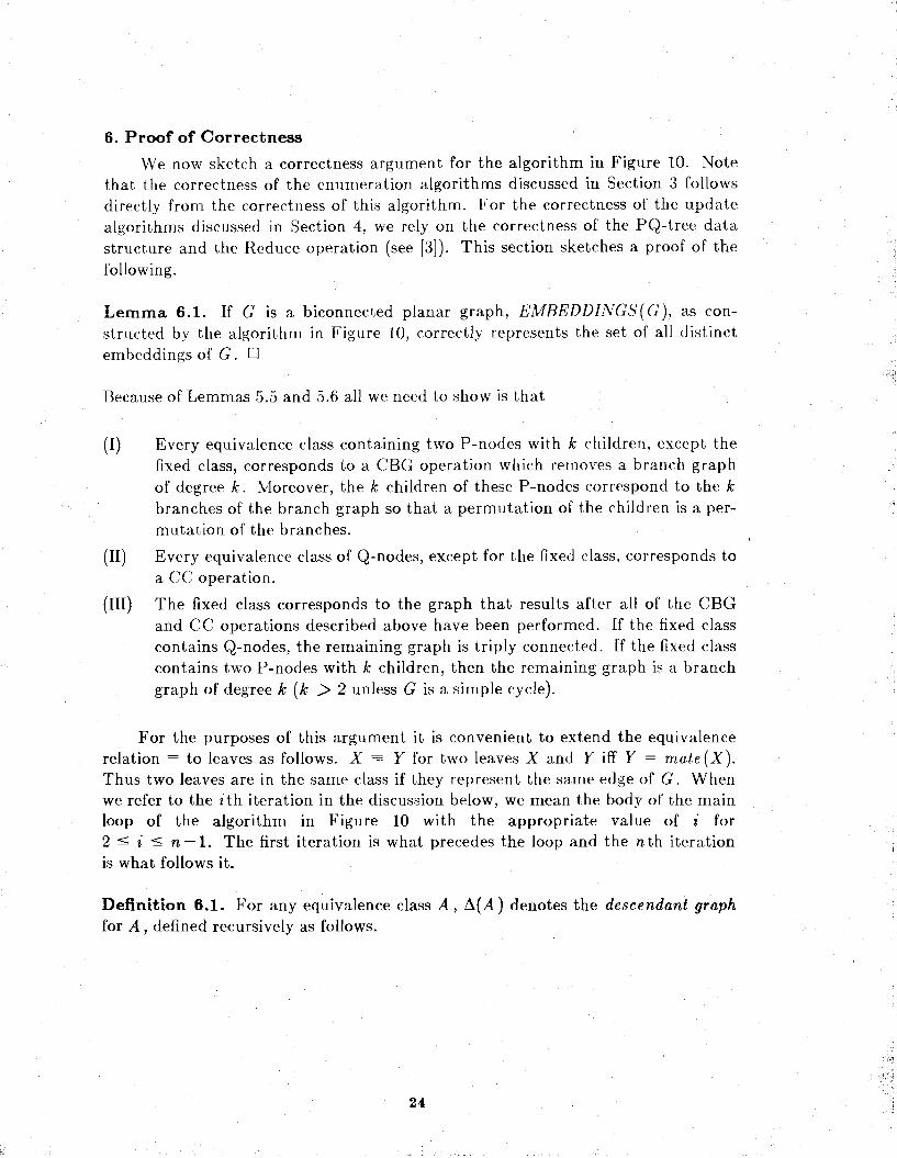
6. Proof of Correctness

We now sketch a correctness argument for the algorithm in Figure 10. Note that the correctness of the enumeration algorithms discussed in Section 3 follows directly from the correctness of this algorithm. For the correctness of the update algorithms discussed in Section 4, we rely on the correctness of the PQ-tree data structure and the Reduce operation (see [3]). This section sketches a proof of the following.

Lemma 6.1. If G is a biconnected planar graph, EMBEDDINGS(G), as con- structed by the algorithm in Figure 10, correctly represents the set of all distinct embeddings of G . U

Because of Lemmas 5.5 and 5.6 all we need to show is that

Every equivalence class containing two P-nodes with k children, except the fixed class, corresponds to a CBG operation which removes a branch graph of degree k. Moreover, the k children of these P-nodes correspond to the k branches of the branch graph so that a permutation of the children is a per- mutation of the branches.

Every equivalence class of Q-nodes, except for the fixed class, corresponds to a CC operation.

The fixed class corresponds to the graph that results after all of the CBG and CC operations described above have been performed. If the fixed class contains Q-nodes, the remaining graph is triply connected. If the fixed class contains two P-nodes with k children, then the remaining graph is a branch graph of degree k ( k > 2 unless G is a simple cycle).

For the purposes of this argument it is convenient to extend the equivalence relation = to leaves as follows. X == Y for two leaves X and Y iff Y = mate (X). Thus two leaves are in the same class if they represent the same edge of G . When we refer to the zth iteration in the discussion below, we mean the body of the main loop of the algorithm in Figure 10 with the appropriate value of i for 2 5 i 5 n - 1. The first iteration is what precedes the loop and the n th iteration is what follows it.

Definition 6.1. For any equivalence class A , A(A) denotes the descendant graph for A , defined recursively as follows.

A(A ) = the edge represented by X ? A if A contains leaves (the edge is interpreted relative to G( i ) during the i th iteration)

A(A) = (I) A(B): Y (: 5 is a child of X C A somewhere in the forest) if A contains interior nodes

Define uJA ) = min V(A(A)) and w(A ) = max V(A(A )) (the lowest, respectively highest, numbered vertex occurring in A(A )).

Consider the algorithm applied to the graph of Figure 2, as shown in Figure 11. In relation to the final active tree before the final set of transformations (i.e. wrt G(5) = G), A(A) = G , p ( A ) = 1, A(B) = { d , e , f ,g ,h , i , j} , d B ) = 2, A(D) = {d,e ,h , i , j} , and p (D) = 2. w ( A ) = w(B) = cu(D) = 5. Earlier, right after the operation Reduce(T,S,>), A(A ) = { a , b , c } , but because all edges are inter- preted relative to G(2), b and c are edges of the form (1,3); thus w(A) = 3 a t that point. Finally, consider class B in the forest for the graph in Figure 12: A(B) = { a ,b ,c}, p (B) = 1, a ( B ) = 3.

Lemma 6.2. The following statements are true wrt G ( i ) after Reduce(T,St) and after Replace_Subroot(T,i)) for the algorithm in Figure 10.

(a) If T(A) is the root of the active tree, then A(A) = G ( i ) (modulo the fact that the outgoing edges from vertex i are not added u n t i l after the Replace-Subroot).

(b) If T(B) is a child of T(A) in the active tree, A(B) A(A) and V(A(A) - A(^?)) f-) ^(A(B)) C W ) , i , i + 11.

(c) If T(A) and T(B) are siblings in the active tree, A(A) A(B) = 0; further-

more V(A(A )) F) V(A(B)) {p(A ) , i , i + I}, and the intersection includes p (A) only if ^ ( A ) = d B ) .

(d) If T(A ) is a full node in the active tree, V(A(A )) includes i but not i + 1, that is u ( A ) = i.

(e) If T(A) is an empty node in the active tree, V(A(A)) includes i + 1 but not i .

(f) If T(B) is a child of T(A) anywhere in the forest, then {p(B),m(B)} + {P(A ),m(A 11.

(g) If T(A) and T(B) are children of the same Q-node T(C) , then the sets MA),m(A)}, {p(B),w(B)}, and {p(C),w(C)} are all distinct.

n The main purpose of Lemma 6.2 is to set the stage for showing that A(A) can be separated from the rest of G by a least split when T(A) is a full node in the active tree or an interior node other than the root in the final active tree. Ultimately, we can carry out CBG and CC transformations by using these least splits in bottom up order relative to the active tree. For the induction arguments below, we want

to be able to show that a least split exists wrt G( i } . This may not be the case, however, even if a least split exists wrt G . The collapsing of vertices 2 + 1 through n may turn G ( i ) - A ( A ) into an isolated path. This observation motivates the following definition.

Definition 6.2. A quasi-least-split of G ( i ) is a semi-split with separation pair x l y } such that of G ' is not an isolated path and has no semi-split with separation pair {x, y }. Furthermore i + 1 $ V(G") - V(A(A )).

If vertex n is not a degree 2 vertex, it is easy to see that any quasi-least-split wrt G( i ) for 1 5 i 5 n - 1 is a least split wrt G .

L e m m a 6.3. If T(A) is an interior node not in the active tree a t the end of itera- tion i (2 5 i n - I ) , then there is a quasi-least-split G ' ( 2 ) = A ( A ) 1) G" with

separation pair { p ( A ) ,(o(A )}.

Proof. Because of Lemma 6.2 (b),(c), and (d), it is clear that A(.4 ) was one com- ponent of a semi-split of G(h) with separation pair {^(-I ) ,h} right before Replace_Subroot( T,h), the operation that removed T(A ) from the active tree (h = w ( A ) 5 i). This semi-split is a quasi-least-split. A ( A ) cannot be an isolated path because r (A) has a t least two children. No semi-split of A(\-{ ) has separation pair {p(A ) ,h} because of Lemma 6.2 (e) and (f ) . 0

Lemma 6.4. If T(A) is an interior node other than the root in the final active tree (after Rotate), then there is a least split G = A(A) I) G" with separation pair

{P(A ),n}.

Proof. Similar to the previous lemma, except that now we rely on the fact that the root has at least two children # T ( A ) to ensure that G - A ( A ) is not an iso- lated path. D

Definition 6.3. The edge graph of A , F(A), is defined (during iteration a ) by per- forming the following transformations on A(A ).

(i) If A(A ) = G ' IJ G" is a quasi-least-split wrt G( i ) , then replace G ' by a sin- gle edge connecting the two vertices of the separation pair.

(ii) If T ( B ) is a child of T(A), then replace A(B) by a single edge connecting d B ) to ~(5).

For the final active tree depicted in Figure 11 (for the graph of Figure 2), r ( D ) = A(D) = {d,e ,h , i , j} , r ( B ) = {f ,g,k}, where A: is the edge from 2 to 5 that was added to replace A(D) (note that r ( D ) is removed from G by a CC transfor- mation in Figure 13(a)), and F(A) = {a,b , c ,l}, where 1 is the edge from 2 to 5 that was added to replace A(B) (note that r ( B ) is removed from G by a CBG

transformation in Figure 13(b)). Note that F ( A ) and F(B) are branch graphs, while r ( D ) 1) { A ; ] is triply connected.

Lemma 6.5. The following are true after Replace_Subroot(T,i).

(a) If A contains two P-nodes with k children, then F(A) is a branch graph of degree k between the vertices p(A ) and oj(A ).

(b) If A contains Q-nodes then F(A) 1) {(p(A),w(A))} is triply connected.

Sketch of Proof. First consider the effect of ReplaceSubroot(T,i) . If T(A) in the active tree has both full and empty children, it loses its full children. However, because of Lemma 6.3, the effect of rule (ii) in Definition 6.3 for the full children is taken over by rule (i). A(A) also gains an edge from vertex i to vertex i + 1 (rule (ii) applied to the new universal tree). If ?(A) is a P-node, the new edge merely adds an extraneous vertex to a branch of a branch graph (there is only one full child in this case). If T(A) is a Q-node, then the new edge is crucial for part (b), as we shall see below.

We now consider how (a) and (b) are affected by Reduce(T,St).

Suppose T(A) is a P-node. From templates that alter children of P-nodes it is easy to see that any child T(B) of T(A) either has d B ) = p (A) or there is a single edge in F(A) between d B ) and P(A) which is either an edge of G or is derived by rule (i) of Definition 6.3. The invariance of part (a) of the lemma under Reduce now follows directly from rule (ii) of Definition 6.3.

The analysis of part (b) under Reduce is much more complicated since the structure of Q-node classes is altered in many ways by the templates.

First note that when Reduce(T,S$) does anything to Q-node equivalence classes, the subroot after Reduce is always a Q-node. The subroot may have been a P-node before the templates were applied. (For example, consider the template (P4) (see Figure 3). The P-node from class A is the original subroot. However, after the template is applied, the new subroot is the Q-node from class B , because all full nodes are descendants of it.) Furthermore, all other Q-nodes created or altered by templates during Reduce are merged into this subroot. We refer to the subroot after application of all templates as the dominant Q-node and the Q-nodes that are merged into it as subordinate Q-nodes.

The following invariant is true a t any stage of the Reduce (i.e. before and after any legal template is applied) for any subordinate Q-node T(B).

* ) GB = r ( B ) I) {( i , i+l ) , (P(B) ,h)} is either triply connected or a branch graph of degree 3, where h may be either i or i + 1. (Note: the edge (p (B) ,h ) is not added to GB if both (p (B) , i ) and ( p ( B ) , i + I ) are present in V(B)). Furthermore, the path p ( B ) h j, where j = i + 1 if h = i and vice versa, is

not an isolated path in GB.

* ) is true if T(B) was a Q-node previous to the Reduce. F{B) differs from its definition during the previous iteration only in that vertex 2 has been split into i and z 4- 1. The edge ( i , i + 1) ensures t ha t is triply connected just as r ( B ) was. Because of the fact that T(B) has at least one full and one empty child the undesir- able isolated path is avoided. In the case of template (P3), the only template that creates a new subordinate Q-node (see Figure 3), F(C) consists of the edges (p (C) , i ) and ([ i(C), i+ 1). Either choice for h yields a branch graph of degree 3 for Gc. The isolated path is avoided in both cases.

The remainder of the argument is in two phases. First we need to show that property (*) is invariant under templates (P5) and (Q2). These are the only tem- plates that alter r (B) when T(B) is a subordinate Q-node. Then we need to estab- lish the lemma for the dominant Q-node under templates (P4), (P6), (QZ) , and (Q3), given that (*) holds for all subordinate Q-nodes and that the graph will ulti- mately include the edge ( i , i+ 1). Instead of presenting all the details, which are rather tedious, we sketch out one of the arguments in each phase. The remaining arguments are similar.

Figure 14 shows the changes that take place in Gn as a result of template (P5) for the special case when s = r (i.e. there are no full children of t,he F-node from class A ) and h = i + 1 for Gn before the application of the template. Lemma 6.2 ensures that v = p(A ) # w = d B ) . Thus the edges ( v , i + 1) and ( v , w) are added to r ( B ) (and w becomes the new d B ) ) . It is now easy to see that after the tem- plate is applied, GB = ^{B) ^J {( i , i+l ) , (v , i )} satisfies (*) (to see that it's triply connected, note that the new Gn is derived from the old by placing vertex v in the middle of the edge ( ru , i+l ) and connecting it to vertex i -- an adaptation of [19, Theorem IV.161). If the P-node from class A has full children but no empty chil- dren, the argument is symmetric: we choose h = i + l instead (the argument is the same for either choice of h in the old Gn). If it has both full and empty children, no edge of the form (v ,h) is added to Gn.

Figure 15 shows the effect of the (Q3) template. We note first that edges corresponding to the children e l l - * - e and f , f can be ignored in the argument. Because of Lemma 6.2 (e) and (f) and an adaptation of [19, Theorem IV.111 such edges can always be added later without affecting the fact that graph is triply connected. The situation illustrated in Figure 15 shows the choice h = z for both Gn and Gp (the argument is similar with other choices of h). GA = r f ( A ) (I {(p(A),co(A))}, where F'(A) is F(A) from the previous iteration. We are ignoring the cases where T(B) or T ( C ) or both are missing (the simplest case of (Q3) is [ e l f , f eJ,, where no change takes place). These are simpler to analyze than the one pictured in Figure 15.

Note that the second part of (*) is critical. If d B ) i i + 1 is an isolated path in r ( B ) then there is a split with separation pair {p(B), i+l} in

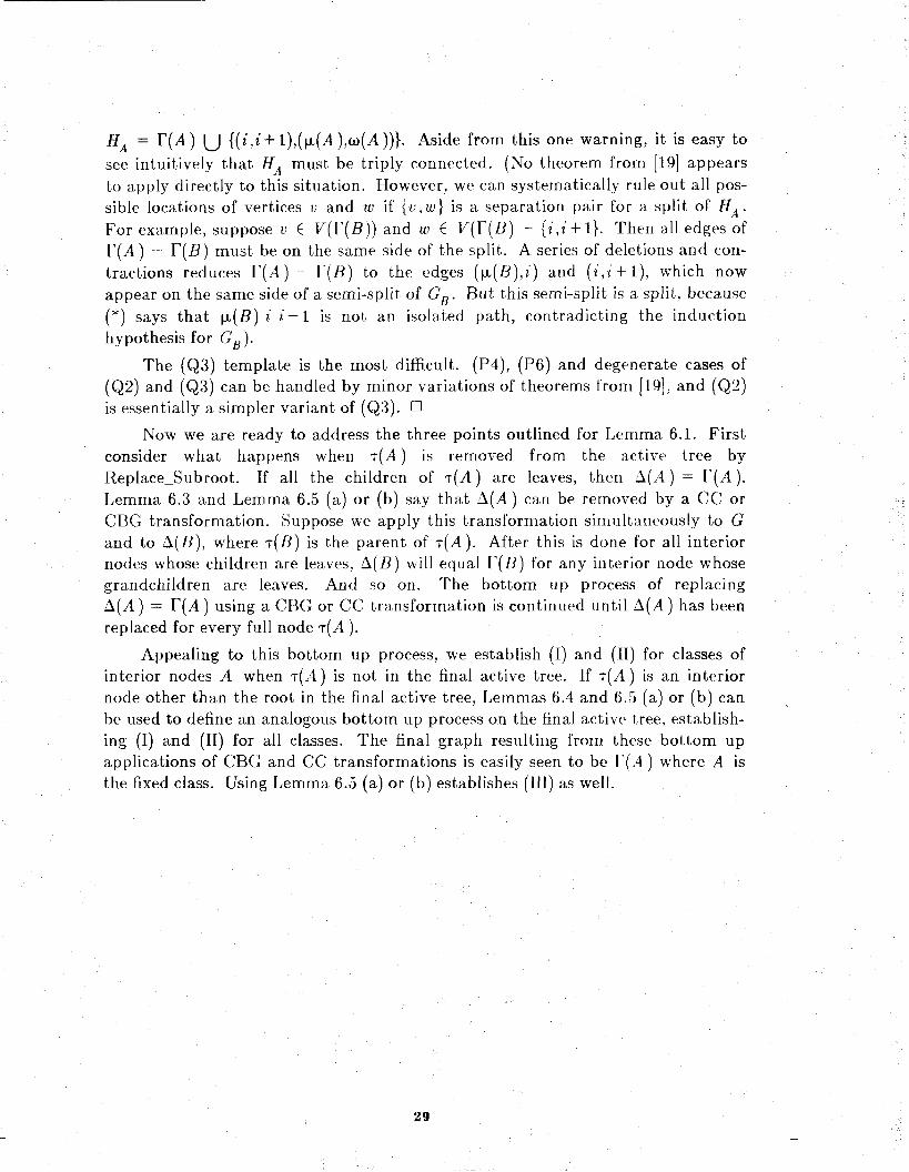
HA = r ( A ) U {(ill '+ l),(p,(A ) , u ( A ))}. Aside from this one warning, it is easy to see intuitively that HA must be triply connected. (No theorem from [19] appears to apply directly to this situation. However, we can systematically rule out all pos- sible locations of vertices v and w if [v, w } is a separation pair for a split of H A . For example, suppose v ? V(I ' (B ) ) and w $ V ( r ( l 3 ) - {2,2+ I}. Then all edges of F(A) - r ( B ) must be on the same side of the split. A series of deletions and con- tractions reduces H A ) - HA?) to the edges (p (B) , i ) and (i,z+ l), which now appear on the same side of a semi-split of G. But this semi-split is a split, because * ) says that ( J L ( B ) 2 i + 1 is not an isolated path, contradicting the induction hypothesis for G n ) .

The (Q3) template is the most difficult. (P4), (P6) and degenerate cases of (Q2) and (Q3) can be handled by minor variations of theorems from 1191. and (Q2) is essentially a simpler variant of (Q3). 0

Now we are ready to address the three points outlined for Lemma 6.1. First consider what happens when T(A) is removed from the active tree by Replace-Subroot. If all the children of T(A) are leaves, then A ( A ) = r ( A ) . Lemma 6.3 and Lemma 6.5 (a) or (b) say that A(A ) can be removed by a CC or CBG transformation. Suppose we apply this transformation simultaneously to G and to A ( B ) , where T(B) is the parent of T ( A ) . After this is done for all interior nodes whose children are leaves, A ( B ) will equal F{B) for any interior node whose grandchildren are leaves. And so on. The bottom up process of replacing A(A) = r ( A ) using a CBG or CC transformation is continued until A ( A ) has been replaced for every full node T(A ).

Appealing to this bottom up process, we establish (I) and (11) for classes of interior nodes A when ? ( A ) is not in the final active tree. If T(A) is an interior node other than the root in the final active tree, Lemmas 6.4 and 6.5 (a) or (b) can be used to define an analogous bottom up process on the final active tree, establish- ing (I) and (11) for all classes. The final graph resulting from these bottom up applications of CBG and CC transformations is easily seen to be F(.4 ) where A is the fixed class. Using Lemma 6.5 (a) or (b) establishes (111) as well.

7. O p e n P rob l ems

We assumed a t the outset that the input graph G was always biconnected. For planarity testing algorithms this assumption is not problen~atic because it is well known that a graph is planar iff all of its biconnected components are planar (see e.g. [19, Theorem XI.211). It is also not too difficult to obtain a planar embed- ding of a graph given planar embeddings of all of its biconnected components. The following Lemma gives a necessary and sufficient condition for a clockwise ordering of edges around each vertex to be an embedding given that the possible embed- dings for all biconnected components have been specified.

L e m m a 7.1. A set of clockwise orderings around each vertex represents an embedding iff ( i ) the subsequences corresponding to each biconnected component specify an embedding for that component, and (ii) no clockwise edge list has a subsequence of the form e f e ' f ', where e and e ' are in one biconnected component and f and f ' are in a different component.

Proof . It is easy to see that every embedding must satisfy condition (i). Suppose condition (i i) is not satisfied, i.e. some vertex v has a clockwise edge list with the forbidden subsequence e f e ' f '. By a series of deletions and contractions of edges, we can reduce the graph to one consisting of just the four critical edges (it is easy to see that deletions and contractions preserve planar embeddings), with e and e ' ending a t vertex w while f and f ' end a t x . Removal of ui and i leaves two loops around vertex v in a configuration that clearly cannot be a planar embedding.

To construct an embedding of a graph G from a set of clockwise edge lists that satisfies (i) and (i i ) , begin with any vertex v. Because of (ii), some biconnected component C for which v (: V(C) has all of its edges around v appearing contigu- ously in the clockwise ordering. Suppose C's edges all appear between e and f in the clockwise order around v , where e and f are arbitrary edges incident to v ( e and f may be the same). Suppose also that embeddings specified by the clockwise ordering have been found for both C and G - C . Then the embedding of C can be placed entirely within the face bounded by e and f of the embedding of G - C. The embedding of C must exist because of (i). We can apply this tech- nique inductively to get the embedding of G - C. 0

This lemma can be used to extend solutions for the problems of constructing a single embedding or verifying an embedding from biconnected graphs to arbitrary graphs. Unfortunately, the OFEC and ONEC problems in their most general form do not appear to have simple solutions based on the above. The difficulty lies in maintaining information about constraints that cross component boundaries.

The enumeration problems also appear difficult when extended to arbitrary graphs. So far the author has been unable to discover the right trick for counting sequences that avoid the forbidden combinations of Lemma 7.1 and satisfy the con- straints within each component without counting identical embeddings twice. When the graph is not biconnected. Definition 1.1 has some ambiguities. It is not

clear, for example, whether two face boundaries should be considered the same if they include the same set of edges or only if they traverse the edges in the same order. The latter seems easier to work with.

By far the most interesting collection of open problems raised by this investi- gation is the problem of maintaining the set of planar ernbeddings for a graph when different kinds of contraints are introduced or even when the graph itself is modified. One problem of this kind is the problem of maintaining the set of embeddings when edges are inserted into or deleted from the graph. Even if we restrict our attention to insertions only, there appears to be no easy solution that is asymptotically faster than 0 ( n ) per insertion.

Deletions in general might cause a biconnected graph to be no longer bicon- nected, thus introducing difficulties already alluded to above. However, it may be fruitful to consider deletions in the following setting: Given a, planar graph G whose set of ernbeddings is represented in a suitable way and an edge e i G, determine whether e can be added to G in such a way that at most one edge needs to be deleted from G and if so perform the swap (if e can be added without delet- ing any edges, it is merely inserted).

References

Alok Aggarwal, Maria Klawe, David Lichtenstein, Nathan Lineal, and Avi Widgerson, "Multi-layer grid embeddings," Proc. 26th Ann. IEEE Symp. on Foundations of Computer Science (Portland, 1985), 186-196.

B.S. Baker, "Approximation algorithms for NP-complete problems on planar graphs," Proc. 2&h Ann. IEEE Symp. on Foundations of Computer Science ( I E E E , 1983), 265-273.

K.S. Booth and G.S. Lueker, "Testing for the consecutive ones property, interval graphs, and graph planarity using PQ-tree algorithms," JCSS 13 (1976), 335-379.

N. Chiba, T . Nishizeki, S. Abe, and T . Ozawa, "A linear algorithm for embedding planar graphs using PQ-trees," JCSS 30 (1985), 54-76.

S. Even and R.E. Tarjan, "Computing an st-numbering," Theoretical Com- puter Science 2 (1976), 339-344.

Danny Dolev, Tom Leighton, and Howard Trickey, "Planar embedding of planar graphs," Advances in Computing Research, vol. 2 (JAI Press, 1984), 147-161.

G.N. Frederickson, "Shortest path problems in planar g raphs ,Vroc . 24th Ann. IEEE Symp. on Foundations of Computer Science ( I E E E , 1983), 242- 247.

L. Heath, "Embedding planar graphs in seven pages," Proc. 25th Ann. IEEE Symp. on Foundations of Computer Science (IEEE, 1984), 74-83.

J.E. Hopcroft and R.E. Tarjan, "Isomorphism of planar graphs (Working paper)," in Complexity of Computer Computations, Miller and Thatcher, eds. (Plenum, 1972), 131-152.

J.E. Hopcroft and R.E. Tarjan, Tfficient planarity testing,"JACM 21 (1974), 549-568.

J.E. Hopcroft and J.K. Wong, "Linear time algorithm for isomorphism of planar graphs (Preliminary report)," Proc. 6th Ann. ACM Symp. on Theory of Computing, ( A C M , New York, 1974), 172-184.

D.E. Knuth, The Art of Computer Programming, Volume 1: Fundamental Algorithms (Addison Wesley, 1969).

A. Lempel, S. Even, and I. Cederbaum, "An algorithm for planarity testing of graphs," in Theory of Graphs: International Symposium: Rome, July, 1966 P . Rosenstiehl, ed. (Gordon and Breach, New York, 1967), 215-232.

R.J. Lipton and R.E. Tarjan, "Applications of a planar separator theorem," SIAM J. Computing 9 (1980), 615-627.

S. MacLane, "A structural characterization of planar combinatorial graphs," Duke Math. J. 3 (1937), 460-472.

3 2

[16] James A. Storer, "The node cost measure for embedding graphs on the planar grid," Proc. 12th Ann. ACM Symp. on Theory of Computing (Los Angeles, 1980), 201-210.

[17] H. Suzuki, T. Nishizeki, and N. Saito, ftMulticommodity flows in planar undirected graphs and shortest paths," Proc. 17th Ann. ACM Symp. on Theory of Computing ( A C M , New York, 1985), 195-204.

[18] R.E. Tarjan, Data Structures and Network Algorithms (SIAM, 1983).

[19] W.T. Tutte, Graph Theory (Addison Wesley, 1984 ) .

[20] Leslie G. Valiant, "Uni~ersalit~y condiderations in VLSI circuits," IEEE Trans. on Computers, C-30, 135-140 (February, 1981).

[21] S.M. Young, "Implementation of PQ-tree algorithms," Master's thesis, Dept. of Computer Science, University of Washington, 1977.

Figure 2.

[note: templates (PO), (Pi), (QO), and (Ql ) are trivial]

(P2) (applies only when the P-node is ROOT(T,S ' ) )

< e l e , f l fq>. - < e l e < f l . * . f q > Ã ‡ > P

(P3) (doesno tapp ly i f theP-node i s R O O T ( T , S r ) ) < e , - - . e p f l . a f s > ^

" . e p > A < f l

variations on (P3) (variations on other templates are analogous)

(applies only when the P-node is R O O T ( T , S r ) )

(does not apply if the P-node is ROOT ( T ,S ')) cel . ' . e p I eP+i . ' . eq f ' ' ! , I B ' f S > A - [ < e l . - - e P H , f 1 . . - f r

(applies only when the P-node is ROOT ( T , S t ) )

(note: equivalence class C is merged into B)

Ie l . . * e p IeP+l ' - . e q f l f r l B . * ' / . I A - [ e l - - - e p ^ + 1 - - - eq f - . . f , f , + l - - - f . 1 , (note: equivalence class B is merged into A )

(applies only when Q-node is R O O T ( T , S r ) ; either or both of the Q-nodes subscripted B and C may be missing)

[ ' I . a . e p eq f l f A B f t + l . * ' f u

[ f u + l f v '.+I e r I ~ ^ r + l es\A . . .

[ e l a - - ep ^ + I eq f l f t f t t l f u

f u + l f " e q + l . . .

er ^ + I e81A (note: equivalence classes B and C are merged into A )

Figure 3. Templates for the Reduce algorithm.

Figure 4.

(c)

Figure 4.

Figure 5 .

procedure All-Embeddings ( L ) is

/* L is a list of equivalence classes wrt = First and Rest return, respectively, the first element and the remaining ele- ments of a list. * /

if L = 0 then for each vertex i do

print In(i) followed by the reverse of Out ( i ) /* use the current permutation for each P-node and list the children

of each Q-node from left to right */ end do

else A := First(L) if A contains Q-nodes then

All_Embeddings(Rest(L)) if A is not the fixed class then

for X ? A do reverse the order of children of X (swap end children)

end do All_Embeddings(Rest(L ))

end if else

/* A contains two P-nodes X and X ' each having k children */ if A is not the fixed class then

for every permutation IT of 1 , . . . , k do permute the children of X and X' using IT

All-Embeddings(Rest(L )) end do

else /* A is the fixed class */ for every permutation IT of 1, ..., k with ~ ( 1 ) = 1 and

4 2 ) < T ( k ) do permute the children of X and X ' using TT

All_Embeddings(Rest(L )) end do

end if end if

end if end All-Embeddings

Figure 6. Algorithm for generating all embeddings of a graph.

/* The following algorithm processes the compound constraint

{(e f u ]), . - - , (ek, f k , vk)}. -Y is a new Q-node that serves as a representative for the class of the compound constraint.

The procedure D_Reduce(T,e , f ) is a modified form of Reduce. It returns a Q- node Q , which is the new subroot after T is reduced wrt {e , f }, and a boolean flag. The latter is true iff e is to the left of f among the children of Q . Q = 0 indicates that the reduction failed. * /

for i = 1 to k do if el , f C In ( v l ) then

(Y,reverse) := D_Reduce(T(ln(z~,)),el, f l ) if Y = 0 then

if T ( O u t ( u ) ) does not exist then ( Y ,reverse ) : = D-Reduce( T (In ( v ) ) , e l 'right *) (V,reverse) := D_Reduce(T(In(vl)), *left*, f l ) /* Note that in this case, Y is always the special Q-node holding

the *left * and *right* markers and reverse will always be false. */

else halt and report that the constraint cannot be satisfied

end if end if if Y # 0 then

Merge(X, Y,reverse ) else

halt and report tha t the constraint cannot be satisfied end if

else if e l f C Out ( v ) then /* Same as previous case with el and f l switched around. The roles of

I n ( v ) and O u t ( v ) are revered also. */

else if e â I n ( v ) and f l â Out ( u , ) then ( Y ,reverse) := D_Reduce( T (In (vl)),el, *right *) if Y # 0 then

Merge(X, Y ,reverse) else

halt and report tha t the constraint cannot be satisfied end if (Z,reverse) := D_Reduce(T(Out (v1)), f l , *right*) if Z # 0 then

Merge(X,Z,reverse ) else

Figure 7 (page 1)

halt and report that the constraint cannot be satisfied end if

else /* e 6 Out ( v ) and f 6 I n f v , ) * / ( Y , r e v e r s e ) := D_Reduce( T(In(v^) , * l e f t * , e , ) if Y # 0 then

\'Ierge(X, Y , rever se ) else

halt and report that the constraint cannot be satisfied end if ( 2 , r e v e r s e ) := D_Reduce(T(Out(v,)),*left*, f , ) if Z # 0 then

Merge(.V,Z, reverse ) else

halt and report that the constraint cannot be satisfied end if

end if end do

Figure 7. Algorithm for processing a compound constraint.

Figure 7 (page 2)

/* r u n k ( X ) , initially 0 For every Q-node X , is an indicator of the size of the tree containing X when .V" is the root * /

procedure Merge(A', Y ,reverse) is (Ao,rx) := Find(A') ( Y o , r y ) := Find( 1') if -Yo = Y o then

if rx 63 r y $8 reverse # 0 then /* @ is exclusive or * / halt and report inconsistency end if

else if rank (X) 2 rank ( Y ) then

P A R ( Y ) := X if rank(X) = rank( Y ) then

r a n k ( X ) := r a n k ( X ) + 1 end if else

P A R ( X ) := Y end if

end if end Merge

function Find(X) is /* find the root of the tree containing X */ XP := x while XP # PAR ( X P ) do

XP := PAR ( X P ) end do XR := XP /* compress the path from X to XR, the root */ XP := x while XP # XR do

X Q := PAR(3-P) P A R ( X P ) := XR X P := X Q

end do return X R

end Find

Figure 8. The Merge algorithm.

Out {{): [*left* <a b c >,

In (2): [ *left * a *right *] ;

In(3): [*left* d 'right*}.,

In(4): [*left* [h e l n *right

Ini t ial forest .

*riqht *]

Out (2):

Out (3):

* 1 ; Ou t (4 ) : [ * l e f t * j

In(5): ["left* <<f g [ i jIB>,. b c>*. *riqht*In;

Initially there are 12 distinct embeddings ( A is the fixed class)

Processing the compound const ra int .

The compound constraint is { (a . f ,2),(b, j , 5 ) } . (the new Q-node class is E )

Changes during the processing of ( a , f ,2) -- D_Reduce( T ( I n (-2)), a , *right *) Merge(£' D ,fa/.se) D_Reduce( T (0ut(2)) , f , *right*)

template ( ~ 3 ) - [*left* [ < g [d elo >c f I F *right*]D In(5): ['left* <[<g [i J I B >Ã f I, b c >,

template (Q2) - [*le f t * <g [d e}g > f *right *] Merge(D , F ,false )

Merge(£ D ,false ) There are now only 8 distinct embeddings (Class C has only 2 children).

Changes during the processing of ( b , j ,5) -- D_Reduce( T (In (5)), b , J )

template (P5) - [ *left * <[[g i j ] f I F b c > A *right *] Out(2): [*le f t * [g [d e IB lB f *rgght*ID

template(Q2)- [* le f t*<[ j i g f I F b c > ^ *right*ID Merge(F ,B,true )

template (P4) - [*left* <\b j i g f\p c > A *right *] F is the new fixed class (in place of A ) Out(1): [*left* < [ b aIF c >, *right*\^

Merge(E , F ,false ) There is now only one distinct embedding. (note: the children of nodes in class B appear in reverse order)

Figure 9. Example showing processing of a compound constraint.

procedure Embed ( G ) is

/* Produces a set of In and Out trees for EL\tBEDD1NGS(G) ( G has n ver- tices), an equivalence relation = among interior nodes of the forest, the special class Fixed, with respect to which orientations are defined, and a list L ( G ) of all the classes that are used in enumerating the embeddings of G . The vertices of G are assumed to be numbered according to an st- numbering (i.e. G is biconnected). Vertex n is required to have degree > 3 unless G is a simple cycle. * /

/* Initialize the active tree T. */ T : = Create-Universal-Tree (1) for i = 2 to n - 1 d o

S = leaves of T representing edges to vertex i T := Reduce ( T , S ) if T = 0 then

halt (the graph is not planar) e n d if Replace-Subroot ( T , a )

e n d d o

L (G ) : = all equivalence classes wrt == except the one containing the root of T if root of T is a P-node with 2 children, not both leaves t h e n

Rotate(T) e n d if I n ( n ) := T Fixed := equivalence class of root of T

e n d Embed

funct ion Create-Universal-Tree ( i ) returns PQNODE is

/* Returns a tree representing the initial constraint on edges from vertex i, namely that they all appear consecutively. The initial tree for Out( i ) is a clone of this new tree, linked to it by the mate relationship. */

El = edges from vertex i if I E , I = 1 t h en

e := the single edge in El Out ( i ) := e r e t u r n a leaf repesenting e

else create a new P-node p create a new P-node p ' make p = p' fo r e â El do

Figure 10 (page 1)

create a new leaf z representing e create a new leaf d representing e m a t e d ) := x'; m a t e ( x r ) := x parent (4 : = p; parent (x ' ) : = p '

end do O u t ( i ) := p' return p

end if end Create Universal Tree

procedure Replace-Subroot ( T , i ) is

/* Replaces the full descendants of R O O T ( T I S ) with a tree representing the initial constraint on the edges from vertex i . The full subtree which is removed in this process is stored as the tree for In ( i ) . * /

p := Create-Universal-Tree ( 1 )

r := ROOT(T,S,) if r is a Q-node with empty children then

/ * the identity of r is not necessarily known in this case */ let f - - f , be the full children of r let e be the empty sibling of f , or 0 if it doesn't exist

/* the full subtree needs a new root because ROOT ( T , S t ) has empty chil- dren */

create a new Q-node q children(q) := [f , - . f k ]

Merge (q .parent ( f , ) , l e f t ( / ,) = e,,) I n ( ( ) := q replace f . - f k by p in children(r)

else /* r is a P-node. a leaf, or Q-node with no empty child */ /* p replaces r and r is the root for I n ( i ) . */ parent(p) := parent ( r ) ; mate ( p ) := mate ( r ) if r is the child of a Q-node q then

replace r by p in children ( q ) end if I n ( i ) := r parentir) := 0; mate ( r ) := 0

end if end Replace Subroot

Figure 10 (page 2)

procedure Rotate( T) is

/* Gets rid of the root of T if the root is a P-node with only two children. Assumes that the root has a t least one non-leaf child. * /

z := a non-leaf child of root of T y := the other child of root of T if x is a P-node then

let i ' be the unique node = x /* x' is the root of the tree representing O u t ( i ) for some vertex i # 1 */ make T ( I n ( i ) ) a child of x ' T ( I n ( 2 ) ) := 0

end if make y a child of x make x the root of T remove the class containing i from L ( G )

end Rotate

Figure 10. The embedding algorithm.

Figure 10 (page 3)

Ver tex 1 Active tree: <a b c >,, Out(1): <a b c > A

Ver tex 2 Reduce(T,{a}) is a no-op (the subroot is a leaf) Replace_Subroot( T ,2}

In (2): a Active tree: < < d e f g > B b c > A

Out(2): <d e f g > B

Ver tex 3 Reduce( T , { d } ) is a no-op (the subroot is a leaf) Replace_Subroot( T ,3)

Zn(3): d Active tree: <<<h i > ^ e f g > B b c > ^ Outf3): <h i>^

Vertex 4 Reduce( T , [ e ,h })

template(P3)- < < [ i hID e f g > B b c > ^

Out (3 ) : [i hID template (P4) - < < [ i h e l D f g > B b c >,.,

Out(2): < [ d f g > B

Replace_Subroot( T ,4) In(4): [ h e l D Active tree: < <[i j}^ f g >B b c > A

Out(4): j

Ver tex 5 In(5): < < [ i jID f g > B 6 c > ^ Fixed = A

Figure 11. The embedding algorithm applied to the graph in Figure 2.

In (3) (final active tree):

In (3) (final active tree):

C is the new fixed class, and A is ignored when ernbeddings are enumerated.

(4

Figure 12. A graph for which the final active tree requires rotation.

Figure 13. CC and CBG transformations on the graph of Figure 2.

Before

After

Figure 14. The (P5) template in the proof of Lemma 6.5.

Figure 15. The (Q3) template in the proof of Lemma 6.5.