Generated using V3.2 of the official AMS LATEX template–journal page layout FOR AUTHOR USE ONLY, NOT FOR SUBMISSION!

Practical Estimates of the Ensemble Size Necessary for Particle Filters

Laura Slivinski, ∗

Woods Hole Oceanographic Institution, Woods Hole, Massachusetts

Chris SnyderNational Center for Atmospheric Research, Boulder, Colorado

†

ABSTRACT

Particle filtering methods for data assimilation may suffer from the “curse of dimensionality,” wherethe required ensemble size grows rapidly as the dimension increases. It would therefore be usefulto know a priori whether a particle filter is feasible to implement in a given system. Previouswork provides an asymptotic relation between the necessary ensemble size and an exponentialfunction of τ2, a statistic that depends on observation-space quantities and that is proportional tothe system dimension when the number of observations is large; for linear, Gaussian systems, thestatistic τ2 can be computed from eigenvalues of an appropriately-normalized covariance matrix.Tests with a low-dimensional system show that these asymptotic results remain useful when thesystem is nonlinear, with either the standard- or optimal-proposal implementation of the particlefilter. We also explore approximations to the covariance matrices that facilitate computation inhigh-dimensional systems, as well as different methods to estimate the accumulated system-noisecovariance for the optimal proposal. Since τ2 may be approximated using an ensemble from asimpler data-assimilation scheme, such as the ensemble Kalman filter, the asymptotic relationsthus allow an estimate of the ensemble size required for a particle filter before its implementation.Finally, we demonstrate the improved performance of particle filters with the optimal proposal,relative to those using the standard proposal, in the same low-dimensional system.

1. Introduction

Ensemble methods have been used in a variety of geo-physical estimation problems, including atmospheric appli-cations, oceanography, and land surface systems. Recentlythere has been growing interest in particle filtering meth-ods in particular, as these methods are better able to cap-ture the nonlinearity inherent in many geophysical systems[e.g. the merging particle filter of Nakano et al. (2007), theequivalent-weights filter of Ades and van Leeuwen (2013),and the implicit particle filter (Morzfeld et al. 2012)]. Atthe same time, particle filters also tend to suffer from the“curse of dimensionality” where the required ensemble sizegrows very rapidly as the dimension increases. Thus, itwould be useful to know a priori whether a particle filteris feasible to implement in a given system.

The curse of dimensionality is a well-known problemin density estimation, as Monte-Carlo estimation of high-dimensional probability densities demands notoriously largesample sizes (Silverman 1986). In a series of related papers,Bengtsson et al. (2008), Bickel et al. (2008), and Snyderet al. (2008) show the curse of dimensionality is also man-ifest in simple particle filters. They demonstrate that therequired ensemble size scales exponentially with a statisticrelated, in part, to the system dimension and which may be

considered as an effective dimension. In general, the parti-cle filter allows a choice of proposal distribution from whichparticles are drawn. Snyder and Bengtsson (2015) (see alsoSnyder (2012)) showed that the exponential increase of theensemble size with effective dimension also holds for parti-cle filters using the optimal proposal (Doucet et al. 2001),which we will introduce in more detail in section 5.

We will consider particle filters based on both the pro-posals above. In the case examined by Bengtsson et al.(2008); Bickel et al. (2008); Snyder et al. (2008), the pro-posal is the transition distribution for the system dynam-ics, where new particles are generated by evolving parti-cles from the previous time under the system dynamics. Ityields the bootstrap filter of Gordon et al. (1993) and wastermed the “standard” proposal by Snyder (2012); Snyderand Bengtsson (2015). The optimal proposal is of interestboth because of its relation to the implicit and equivalent-weights particle filters and because it minimizes the degen-eracy of weights, as shown in Snyder and Bengtsson (2015),and thereby provides a bound on the performance of otherparticle filters.

Our ultimate goal is to be able to determine whether aparticle filter would be feasible to implement, given that wehave statistics from, say, a working ensemble Kalman filter.

1

For the standard proposal, this is straightforward: the fore-cast step of ensemble forecasts provides a draw from theproposal and we simply need to compute weights based onthe observation likelihood for each member. However, it isharder to use an existing ensemble to assess the feasibilityof the particle filter based on the optimal proposal, sinceit is non-trivial to develop an algorithm to sample fromthis proposal [c.f. Morzfeld et al. (2012)]. An alternativeis to utilize the results of Bengtsson et al. (2008); Bickelet al. (2008); Snyder et al. (2008); Snyder and Bengtsson(2015) that relate the behavior of the weights in the linear,Gaussian case to eigenvalues of certain covariance matriceswhich may be estimated from an existing ensemble. Weevaluate the use of these results in more general nonlin-ear, non-Gaussian settings. Note that sampling error alsopresents an issue in applying these results; we investigatethese effects and possible methods for overcoming them inthis paper as well.

We note here that Chorin and Morzfeld (2013) have in-vestigated a different, but related, effective dimension ofa Gaussian data assimilation problem. In particular, theydefine a “feasibility criterion” to be the Frobenius norm ofthe steady state posterior covariance matrix (which can beexactly calculated in the linear, Gaussian regime.) Whileboth studies explore potential limitations of particle filter-ing in high-dimensional systems, their criterion is based onbounding the total posterior error variance as a function ofan effective dimension, whereas the studies of Snyder et al.(2008) and Snyder and Bengtsson (2015) quantify the rela-tion between degeneracy of the particle-filter weights andan effective dimension.

The remainder of this paper is organized as follows. InSection 2, we review the ensemble Kalman filter and theparticle filter and their respective implementations. Sec-tion 3 reviews the previous results of Snyder et al. (2008)regarding the limits of particle filters in high dimensionallinear systems. Section 4 verifies the applicability of theresults for linear, Gaussian systems and the standard pro-posal to nonlinear systems; this is specifically useful forunderstanding the similar extension needed for the optimalproposal. In Section 5, we consider the optimal proposalin a nonlinear system and discuss some of the difficultiesthat arise, in particular regarding additive model noise innonlinear systems. Section 6 includes comparisons of per-formance of the standard and optimal proposals in a non-linear system. Finally, Section 7 summarizes the resultsand draws conclusions.

2. Review of Ensemble Methods and Previous Re-sults

Ensemble data assimilation methods approximate prob-ability distributions using an ensemble of states, eitherweighted or unweighted. Two common ensemble meth-

ods are the ensemble Kalman filter (EnKF) and the parti-cle filter. Generally, the traditional EnKF algorithm usesunweighted ensemble members, which are themselves up-dated when an observation becomes available. On theother hand, the particle filter uses a weighted ensemble.When an observation is available, the particles are drawnfrom a proposal distribution and then reweighted accordingto the observation.

In this section, we will first describe the setup and somenotation, and then briefly review the standard and optimalproposal implementations of the particle filter as well as theensemble Kalman filter.

a. Setup and Notation

Assume that our state of interest is given by xk ∈ RNx ,where k indexes time and Nx is the dimension of the state.We will additionally assume that model noise is added atintegration time steps (of size dt) indexed by l below, whileobservations are available every Nt integration steps, in-dexed by k. Let the time between observations be denotedby ∆t = Nt · dt. The model evolution can be described as:

xk,l = m(xk,l−1) + ηl−1, l = 1...Nt, (1)

where xk,Nt = xk+1,0 := xk+1 and observations are avail-able for xk, k = 1, . . . , Nobs. The ηj , whose dependence onk is suppressed for notational convenience, are i.i.d. ran-dom variables that represent the system noise and have adistribution to be specified later. Further define Mstoch tobe the operator that takes xk,0 to xk,Nt . That is, Mstoch

includes the nonlinear convolution of the noise between ob-servation times:

xk = Mstoch(xk−1, η0, . . . , ηNt−1). (2)

In particular, note that the model noise is not additive atobservation times when m is nonlinear. Next assume thatwe have linear, noisy observations of the state given by

yk = Hxk + εk, (3)

where yk ∈ RNy is the observation of dimension Ny andεk ∼ N (0,R) is the observation error. For the followingmethods, we denote unweighted ensembles of size Ne as{xi

k}Nei=1, and weighted ensembles as {xi

k, wik}. Finally,

yk1:k2will denote the concatenation of the observations

from time tk1to time tk2

.

b. Particle filter

The particle filter estimates the true Bayesian prob-ability distributions using a weighted ensemble of states.When an observation is available at time tk, we are inter-ested in p(xk|y0:k) ≈

∑Ne

i=1 wikδ(xk − xi

k). We will brieflyreview the derivation of the weight update based on impor-tance sampling (Doucet et al. 2000; Snyder 2012; Snyder

2

and Bengtsson 2015), which more generally also includesdependence on the state at the previous time: xk−1. Tothis end, suppose we want to sample from the distribu-tion p(xk,xk−1|y0:k), which is unknown. Instead we sam-ple from a proposal distribution denoted π(xk,xk−1|y0:k),which we can choose, and then assign weights to each mem-ber of the sample. We will choose our proposal distributionto be of the form of the product π(xk−1)π(xk|xk−1,yk),which will allow for a recursive definition of the weights.This weighted ensemble is then a sample from the correctdistribution, if the weights are given by

wik ∝

p(xik,x

ik−1|y0:k)

π(xk,xk−1|y0:k)(4)

and normalized to sum to 1. Since we will always be con-ditioning on y0:k−1, we omit this term in what follows, andconsider only yk.

1) Standard proposal

The simplest choice for a proposal density is the stan-dard proposal, in which π(xk|xk−1,yk) is chosen to bep(xk|xk−1). Then, noting thatp(xk,xk−1|yk) ∝ p(yk|xk)p(xk|xk−1)p(xk−1),

wik ∝

p(yk|xik)p(xi

k|xik−1)

π(xik|xi

k−1,yk)wi

k−1 (5)

∝ p(yk|xik)wi

k−1 (6)

where the constant of proportionality is determined so thatall weights sum to 1.

2) Optimal proposal

Doucet et al. (2000) discuss the so-called optimal pro-posal, which includes information about the previous stateas well as the current observation: π(xk|xk−1,yk) =p(xk|xk−1,yk). In this case, the weights are updated ac-cording to:

wik = p(yk|xi

k−1)wik−1. (7)

Sampling from this proposal is discussed in more detail inthe appendix, but note that drawing from the optimal pro-posal and updating the weights are both more complicatedin the case of the optimal proposal than the standard pro-posal. Despite this added computational effort, there arecases in which the optimal proposal has significant per-formance gain over the standard proposal, with the samenumber of particles (see Section 6 below.) Thus the opti-mal proposal may be more computationally tractable thanthe standard proposal in terms of the number of particlesneeded for an acceptable error level.

c. Ensemble Kalman filter

Evensen (1994) introduced the ensemble Kalman filteras an approximation of the Kalman filter which, like theparticle filter, uses an ensemble of realizations of the systemstate to represent probability distributions. Unlike the par-ticle filter, the ensemble Kalman filter uses an unweighted(or equally weighted) ensemble of states. Suppose the en-

semble at time tk is given by {xf,ik }

Nei=1, where f stands for

“forecast,” and a will represent “analysis.” If an observa-tion is also available at time tk, each ensemble member isupdated according to

xa,ik = xf,i

k −K(yk − xf,ik + εik), (8)

K = PfHT (HPfHT + R)−1 (9)

where εik ∼ N (0,R) and Pf is the ensemble covariance ofthe forecast:

Pf =1

Ne − 1

Ne∑i=1

(xf,ik − x̄f

k

), (10)

x̄f =1

Ne

Ne∑i=1

xf,ik . (11)

This is the so-called perturbed-observation formulation ofthe EnKF (Evensen 2003), in which each observation isviewed as a random variable. In the update step, we replaceyk with yk + εk where εk has the same statistics as theobservation error noise. This formulation is shown to givethe correct posterior covariance; otherwise, the covarianceis overly tightened [see Burgers et al. (1998); Houtekamerand Mitchell (1998)].

The EnKF is a linear method, and thus will be sub-optimal for problems that are significantly non-Gaussianeven if Ne is large. However, for distributions which areclose to Gaussian, the EnKF works well with relatively fewensemble members, though often it requires localizationand inflation [see Houtekamer and Mitchell (1998, 2001);Anderson and Anderson (1999); Hamill et al. (2001)]. Inthe experiments in this paper, we use the perturbed obser-vation formulation of the EnKF with covariance localiza-tion using the compactly supported correlation function ofGaspari and Cohn (1999) and a small but fixed inflation.

d. Review of Previous Asymptotic Results

Snyder et al. (2008) prove, in certain regimes, an expo-nential relationship between the variance of the observationlog-likelihood and the inverse of the maximum weight. Inthe linear Gaussian case, this variance can be calculated asa sum of eigenvalues of an explicit function of covariances.First, we give some definitions.

Define the weight update factor in Equation (5) to be

3

w̃ik; that is,

w̃ik =

p(yk|xik)p(xi

k|xik−1)

π(xik|xi

k−1,yk). (12)

Next define τ2 to be the variance of the log of these factorsconditioned on the observations:

τ2 = var(log(w̃ik)|y). (13)

Let wmax denote the maximum weight over the ensemble.Snyder et al. (2008) show that

E[1/wmax]− 1 ≈√

2 logNe

τ, (14)

under the following assumptions: first, that the observationerrors are spatially and temporally independent; second,that Ny and Nx are large; third, that Ne and τ/

√logNe

are large, in the sense that τ/√

logNe → ∞ as Ne → ∞;and finally, that the distribution of log(w̃i

k) over draws of xi

from the proposal is sufficiently close to Gaussian. The firstthree assumptions are easily verified and generally hold inthe systems of interest to this work. The final assumptionis less obvious, and below we investigate situations in whichthis assumption may not hold.

Snyder et al. (2008) apply these asymptotic results tothe particle filter with the standard proposal, where w̃i

k =p(yk|xi

k). Snyder (2012); Snyder and Bengtsson (2015)note that similar arguments apply to the optimal proposal,where w̃i

k = p(yk|xik−1). Snyder and Bengtsson (2015) also

note that the asymptotic theory developed for the optimalproposal provides bounds for the implicit particle filter, asthe implicit particle filter reduces to the optimal proposalparticle filter in the case where observations are linear andtaken every step (Morzfeld et al. 2012). Although we willconsider nonlinear, non-Gaussian systems, the asymptoticsdeveloped in the linear, Gaussian case are of interest herebecause they provide an explicit expression for τ2. Ad-ditionally, in the linear, Gaussian case, the conditions forlog w̃i

k to be Gaussian (and thus for validity of the asymp-totic theory) are straightforward.

We take the linear, Gaussian system to be

xk = Mxk−1 + γk, (15)

where γk ∼ N (0,Q) and the observations are as defined in(3). Note that, for the linear Gaussian case, the dynamicsare only written for observation times tk, in contrast to (1).

With the standard proposal, we first need to calculatethe eigenvalues λ2

j of the matrix

Cs = R−1/2Hcov(xk)HTR−1/2. (16)

Snyder et al. (2008) and references therein derive the rela-tion

E(τ2) =

Ny∑j=1

λ2j

(1 +

3

2λ2j

), (17)

where the expectation is taken over yk. Moreover, Bickelet al. (2008) show that log w̃i

k is asymptotically Gaussian(over draws from the proposal), and the relation (14) isvalid, as long as no eigenvalue(s) dominate the sum ofsquares above. In the case of the optimal proposal, thesame expression (17) and the same conditions for validityhold, but using the eigenvalues of

Co = (R+HQHT )−1/2HMcov(xk−1)MTHT(R+HQHT)−1/2.(18)

In a system where each degree of freedom is indepen-dent and independently observed, these expressions sim-plify and show that τ2 will be proportional to the numberof observations. A similar but more informal derivation ofthis result also appears in Ades and van Leeuwen (2013).

3. Model and Experimental Setup

In all experiments in this paper, we will restrict our at-tention to the nonlinear dynamical system of Lorenz (1996).The deterministic form of these equations is given by:

dx(j)

dt= (x(j+1) − x(j−2))x(j−1) − x(j) + F, (19)

for j = 1, . . . , Nx and F = 8 here. The subscripts (j)indicate the spatial location in a one-dimensional, periodicdomain and should be understood mod Nx.

We solve a discrete-time, stochastic version of this equa-tion, cast in the form (1). Fixing an integration time stepdt and an observation time step ∆t = Ntdt, we computem(xk,l−1) by integrating (19) over a single time step dt us-ing a fourth-order Runge-Kutta scheme and draw ηl−1 fromN (0, dtσ2

sysI). Except where noted below, all results em-ploy dt = 0.01. Alternatively, we could have started from acontinuous time stochastic differential equation by includ-ing noise directly in Eqn. (19); this distinction is not crucialto any of the results we present. The observing networkin the experiments will consist of full observations, so thatH = I, and the observation error covariance is R = σ2

obsI.We will need an example ensemble DA scheme to calcu-

late the statistics necessary to test the asymptotic theory.Since our goal is to demonstrate that these statistics maybe used in practice to determine the applicability of theparticle filter, we will use the EnKF, a common methodfor high-dimensional problems, to calculate the statistics.While the EnKF is suboptimal in the nonlinear case, wewish to show that the method is reasonably effective acrossa wide range of parameters for this system. The spread-skill relation (Table 1) indicates that this is true. For thisexperiment, we fix Nx = 100, let the system noise be fixedwith σsys = 0.01, and vary the observation error noise σ2

obs.For each value of observation error, we run the EnKF for200 sequential observations. Table 1 shows the forecastmean squared error and forecast variance over the last 190observations, for each value of observation error. For these

4

results, ∆t = 0.1. As the results show, the EnKF is work-ing well with the chosen values of inflation and localization,since the forecast mean squared error (MSE) and varianceare comparable and neither blows up.

Table 1. Forecast error and variance of the workingEnKF, with varying values of observation noise.

σ2obs forecast MSE avg forecast var

0.0001 0.0021 0.00110.0005 0.0024 0.00140.001 0.0027 0.00180.003 0.0037 0.00270.005 0.0044 0.00350.007 0.0052 0.00410.009 0.0057 0.00480.02 0.0082 0.00750.05 0.0145 0.01420.1 0.0236 0.02430.5 0.0736 0.08301 0.1448 0.1695

In Section 6, we will run a sequential particle filter formany observations to compare the overall performance ofdifferent proposal algorithms. In this case, we will needto resample in order to prevent weight collapse: here, wetest two different resampling thresholds. The first is the re-sampling threshold defined in Kong et al. (1994), in whichthe filter is set to resample when the effective sample sizeNeff = 1/

∑Ne

i=1(wi)2 falls below a fixed ensemble size Nt.This is the threshold suggested by Arulampalam et al.(2002). The second threshold is based on the maximumweight, in which the filter resamples when wmax exceeds acertain value (here we use 0.5.) We then use a Monte CarloMetropolis-Hastings resampling technique [see (Hastings1970; Robert and Casella 2004) for an introduction and(van Leeuwen 2009) for a description applied to particlefilters], followed by resetting the weights to be equal.

4. Extension to Nonlinear Case: Standard Pro-posal

Our goal is to show how to use an existing DA en-semble to determine whether it would be feasible to use aparticle filter for a given nonlinear system, and if so, howmany particles would be necessary to avoid filter collapse.In the case of the standard proposal, it is straightforwardto directly calculate the weights without implementing theparticle filter and quantify the statistics of the maximumweight directly. Alternatively, if we know R and cov(xk),we could use Eqn. (17) to estimate τ2 and then predictE(1/wmax) from Eqn. (14). This alternative approach topredict the behavior of wmax is especially useful in the case

of the optimal proposal, where computing the weights di-rectly requires sampling from the optimal proposal, whichcan be difficult. Thus we first numerically demonstrate thetheory in the simpler case with the standard proposal, butwith a nonlinear model, before moving on to the optimalproposal. Note that the asymptotics have been verifiednumerically for linear, Gaussian systems in Snyder et al.(2008).

We consider the Lorenz (1996) equations with Nx =100, fix the system noise as σsys = 0.01, and vary theobservation error variance σ2

obs. The existing DA schemewe use is the EnKF as described in Section 3.

First, to demonstrate the degree of nonlinearity in thissystem of equations, we study the difference in perturba-tions after evolving two initial points forward under thefully nonlinear Lorenz equations as well as a linearized sys-tem. Specifically, we choose a random observation time inthe EnKF experiment, choose two random ensemble mem-bers as our initial perturbation, and linearize the systemabout one of them. We evolve each ensemble member un-der the linearized dynamics to get {xi

lin}i=1,2 and underthe full dynamics to get {xi

full}i=1,2; we then measure thelinearity of the system with

err =

∣∣∣|x1full − x2

full| − |x1lin − x2

lin|∣∣∣

|x1full − x2

full|, (20)

where |x1 − x2| =

[∑Nx

j=1

(x1

(j) − x2(j)

)2]1/2

. This will be

close to 0 if the full system is close to linear. Addition-ally, note that this traditional version of the Lorenz (1996)equations with F = 8 has a doubling time of 2.1 days,where one model time unit corresponds to 5 days; thus, thedoubling time is 0.42 model time units. Table 2 shows re-sults with a fixed dt = 0.005, and variable integration time∆t, averaged over 100 randomly chosen observation times.Note that in the experiments in this paper, we vary thetime between observations as ∆t = 0.1 (standard proposalexperiment) or ∆t = 0.4 (optimal proposal experiment,following section.)

The results in Table 2 show that the measure of non-linearity is very close to 0 for a single integration step, butquickly increases for longer time windows. This impliesthat the system is well-approximated by a linear model af-ter just one integration step, but the nonlinearity increasesas the length of integration increases. We have there-fore chosen observation frequencies for the following ex-periments which guarantee nonlinear behavior of the modelbetween observations in order to test the theory. Addition-ally, note that although we are operating in a regime wherethe system is fully observed, based on theory, we expect thesame results to hold in the more realistic situation of in-homogeneous spatial observation coverage. In particular,fewer observations will lead to more strongly non-Gaussian

5

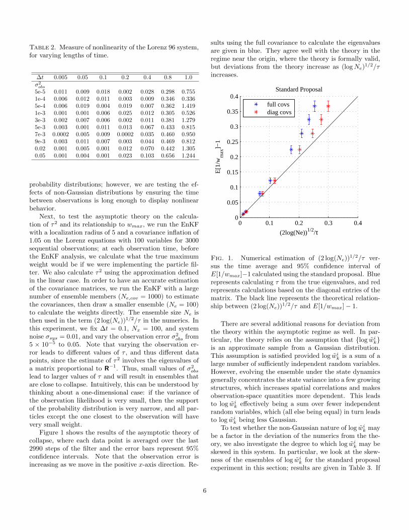
Table 2. Measure of nonlinearity of the Lorenz 96 system,for varying lengths of time.

∆t 0.005 0.05 0.1 0.2 0.4 0.8 1.0σ2obs

5e-5 0.011 0.009 0.018 0.002 0.028 0.298 0.7551e-4 0.006 0.012 0.011 0.003 0.009 0.346 0.3365e-4 0.006 0.019 0.004 0.019 0.007 0.362 1.4191e-3 0.001 0.001 0.006 0.025 0.012 0.305 0.5263e-3 0.002 0.007 0.006 0.002 0.011 0.381 1.2795e-3 0.003 0.001 0.011 0.013 0.067 0.433 0.8157e-3 0.0002 0.005 0.009 0.0002 0.035 0.460 0.9509e-3 0.003 0.011 0.007 0.003 0.044 0.469 0.8120.02 0.001 0.005 0.001 0.012 0.070 0.442 1.3050.05 0.001 0.004 0.001 0.023 0.103 0.656 1.244

probability distributions; however, we are testing the ef-fects of non-Gaussian distributions by ensuring the timebetween observations is long enough to display nonlinearbehavior.

Next, to test the asymptotic theory on the calcula-tion of τ2 and its relationship to wmax, we run the EnKFwith a localization radius of 5 and a covariance inflation of1.05 on the Lorenz equations with 100 variables for 3000sequential observations; at each observation time, beforethe EnKF analysis, we calculate what the true maximumweight would be if we were implementing the particle fil-ter. We also calculate τ2 using the approximation definedin the linear case. In order to have an accurate estimationof the covariance matrices, we run the EnKF with a largenumber of ensemble members (Ne,cov = 1000) to estimatethe covariances, then draw a smaller ensemble (Ne = 100)to calculate the weights directly. The ensemble size Ne isthen used in the term (2 log(Ne))

1/2/τ in the numerics. Inthis experiment, we fix ∆t = 0.1, Nx = 100, and systemnoise σsys = 0.01, and vary the observation error σ2

obs from5 × 10−5 to 0.05. Note that varying the observation er-ror leads to different values of τ , and thus different datapoints, since the estimate of τ2 involves the eigenvalues ofa matrix proportional to R−1. Thus, small values of σ2

obs

lead to larger values of τ and will result in ensembles thatare close to collapse. Intuitively, this can be understood bythinking about a one-dimensional case: if the variance ofthe observation likelihood is very small, then the supportof the probability distribution is very narrow, and all par-ticles except the one closest to the observation will havevery small weight.

Figure 1 shows the results of the asymptotic theory ofcollapse, where each data point is averaged over the last2990 steps of the filter and the error bars represent 95%confidence intervals. Note that the observation error isincreasing as we move in the positive x-axis direction. Re-

sults using the full covariance to calculate the eigenvaluesare given in blue. They agree well with the theory in theregime near the origin, where the theory is formally valid,but deviations from the theory increase as (logNe)

1/2/τincreases.

0 0.1 0.2 0.3 0.40

0.05

0.1

0.15

0.2

0.25

0.3

0.35

0.4

(2log(Ne))1/2/τ

E[1

/wm

ax]−

1

Standard Proposal

full covsdiag covs

Fig. 1. Numerical estimation of (2 log(Ne))1/2/τ ver-

sus the time average and 95% confidence interval ofE[1/wmax]−1 calculated using the standard proposal. Bluerepresents calculating τ from the true eigenvalues, and redrepresents calculations based on the diagonal entries of thematrix. The black line represents the theoretical relation-ship between (2 log(Ne))

1/2/τ and E[1/wmax]− 1.

There are several additional reasons for deviation fromthe theory within the asymptotic regime as well. In par-ticular, the theory relies on the assumption that {log w̃i

k}is an approximate sample from a Gaussian distribution.This assumption is satisfied provided log w̃i

k is a sum of alarge number of sufficiently independent random variables.However, evolving the ensemble under the state dynamicsgenerally concentrates the state variance into a few growingstructures, which increases spatial correlations and makesobservation-space quantities more dependent. This leadsto log w̃i

k effectively being a sum over fewer independentrandom variables, which (all else being equal) in turn leadsto log w̃i

k being less Gaussian.To test whether the non-Gaussian nature of log w̃i

k maybe a factor in the deviation of the numerics from the the-ory, we also investigate the degree to which log w̃i

k may beskewed in this system. In particular, we look at the skew-ness of the ensembles of log w̃i

k for the standard proposalexperiment in this section; results are given in Table 3. If

6

the skewness is far from 0, then the sample distribution isfar from Gaussian. The skewnesses are averaged over thelast 2990 observations. As the results in Table 3 show,larger observation error generally leads to higher skew-ness values; since large observation error corresponds tolarger 2 logNe/τ

2, this may explain why the data pointsdo not follow the theory as well further from the asymp-totic regime. On the other hand, the observed increase inskewness is not very strong, and thus may not be the onlycause of the deviation between numerics and theory. How-ever, the frequent changes of variables needed to derive τ2

prevent a more detailed analysis of this deviation.

Table 3. Skewness of the ensembles of log w̃ik after one

evolution under the Lorenz 96 model for varying magnitudeof observation error; standard proposal experiment. Meanand 95% confidence intervals over final 2990 time steps.

σ2obs mean skewness

5e-5 0.251± 0.0091e-4 0.252± 0.0095e-4 0.271± 0.0091e-3 0.270± 0.0093e-3 0.281± 0.0095e-3 0.290± 0.0097e-3 0.302± 0.0099e-3 0.300± 0.0090.02 0.320± 0.009

In practice, there are difficulties using Eqn. (17) to es-timate τ2. First, computing a covariance matrix from asmall sample typically yields an eigenvalue spectrum thatis artificially steep, with too much variance in leading direc-tions. The corresponding calculation of τ2 will then be toolarge, since it is a sum of higher powers of the eigenvalues.We have therefore chosen a large ensemble (Ne ≥ Nx) inthis experiment in order to estimate the covariances accu-rately and avoid this effect. Second, for large numbers ofobservations and large ensembles, calculating eigenvaluesof these matrices may be computationally prohibitive.

Thus, we also tested this theory using a computation-ally feasible approximation for the eigenvalues ofR−1/2Hcov(xk)HTR−1/2: we assume R and Hcov(xk)HT

are diagonal, so that the eigenvalues are simply the prod-uct of the corresponding diagonal elements of R−1 andHcov(xk)HT . Results with τ2 approximated in this wayare also shown in Fig. 1. The approximation systematicallyunderestimates τ2 data points with the approximation al-ways lie to the right of those using eigenvalues of the fullmatrix (16). 1 Nevertheless, using the approximation of

1Since τ2 is a sum of squares of the eigenvalues of (16) [see (17)]and because the sum of the eigenvalues equals the sum of the diagonal

τ2 in the asymptotic relation gives reasonable predictionsof E(1/wmax), often better than with the unapproximatedτ2, because the underestimation by the diagonal approxi-mation compensates for the overestimation of E(1/wmax)that is, empirically, a property of the asymptotic relationwhen (2 logNe)

1/2/τ is not small. It is not clear whetherthis compensation will be equally effective in other prob-lems.

5. Optimal Proposal

Next, we follow the approach of the previous section,but apply the asymptotic theory to the optimal proposal.Specifically, we wish to use an existing ensemble to eval-uate the feasibility of a particle filter using the optimalproposal. As in the case of the standard proposal above,the evaluation will be limited by the fact that it appliesresults from linear, Gaussian systems in a nonlinear, non-Gaussian setting, and by sampling errors in estimating thenecessary covariance matrices from a finite ensemble. Wewill check these limitations with numerical simulations us-ing the Lorenz (1996) system. For the optimal proposal,there is also an additional issue, in that some of the co-variance matrices involved in the definition (18) of Co donot appear explicitly in the nonlinear problem. We turn tothis issue first.

a. Model noise in nonlinear systems

The matrix Co, whose eigenvalues determine τ2 for theoptimal proposal via (17) in the linear, Gaussian case, in-volves the covariance matrices HMcov(xk−1)MTHT andHQHT . Since the equations (1)-(3) for the nonlinear sys-tem do not specify these quantities, we take the approachof defining them through more general expressions that re-duce to the correct result for the linear, Gaussian case.

To compute the covariance involving the linear dynam-ics M, we first define Mdet(x) = Mstoch(x, 0, . . . , 0) [re-calling that Mstoch in (2) is a function of the state x aswell as the realizations of the noise at each integration stepη0, . . . , ηNt−1]. In the linear case, Mdet(x) = Mx and amore general definition for the desired covariance is

HM cov(xk−1)MTHT = cov(HMdet(xk−1)). (21)

We estimate the right hand side for the nonlinear system byevolving an ensemble of initial conditions from tk−1 usingMdet, applying H and computing the sample covariance.

For the covariance HQHT , there are at least two possi-ble definitions that generalize to the nonlinear system. Thefirst uses

HQHT = cov(Hxk|xk−1), (22)

elements, τ2 will be underestimated by the diagonal approximationwhenever the eigenvalue spectrum is steeper than the sorted list of di-agonal elements. We expect this to be true in many problems involv-ing spatial correlations, with spatially correlated but nearly spatiallyhomogeneous processes being a prime example.

7

which is an identity in the linear case and gives a quantitythat, in the nonlinear case, will depend on xk−1. We canestimate the covariance on the right hand side by startingfrom a given xi

k−1 and computing an ensembleMstoch(xik−1,

η0, . . . , ηNt−1) over realizations η0, . . . , ηNt−1 of the systemnoise. Let Qi be the state-space covariance estimated inthis way. (Recall from Section 3 that H = I in our ex-periments.) A further step would be to compute Q̄ byaveraging the Qi over an ensemble of xi

k−1.The second possible definition relies on

HQHT = cov(HMstoch(xk−1, η0, . . . , ηNt−1)−HMdet(xk−1)).(23)

This expression is again an identity in the linear case – Qcan be written as the sum over contributions from the noisein (1) at each of the Nt model time steps between tk−1 andtk. Beginning from an ensemble of realizations of xk−1, weestimate the covariance on the right hand side above byevolving each member from tk−1 to tk with both Mdet andMstoch, with independent realizations of the system noisein Mstoch, and then taking the sample covariance of thedifferences in xk. We denote this estimate Q̃.

It is not immediately obvious whether one of these defi-nitions is to be preferred. They will agree in the limit of lin-ear dynamics and may differ as nonlinearity increases. Wehave therefore explored the behavior of both approaches inthe case with Nx = 100, ∆t = 0.1, and with varying modelnoise σsys and initial ensemble size σens. The test consistsof evolving the particles forward from time 0 to time ∆tand estimating Q in the three ways described above. First,we calculate Qi for each particle; second, we take the av-erage Q̄ of these Qis; finally, we estimate Q̃ as above. Wefound that the variations of Qi about Q̄ were negligiblerelative to the magnitude of elements of Q̄. Similarly wefound good agreement between Q̄ and Q̃ in these cases.Thus, the effects of nonlinearity in estimating the effectivemodel noise covariance are small in these experiments; inparticular, they are much smaller than sampling error inestimates of Q with ensembles of size 100, which we use inthe following experiments.

The two definitions do, however, differ substantially intheir computational demands, as the computation of the Qi

and Q̄ requires an ensemble of integrations for each xik−1,

while a single integration for each xik−1 suffices for Q̃. In all

following experiments, we therefore use Q̃ to estimate themodel noise covariance, as it is the most computationallyefficient.

b. Numerical Results

Snyder and Bengtsson (2015) have rigorously shownthat the asymptotics developed in Bengtsson et al. (2008);Snyder et al. (2008) also hold for the optimal proposal.Here, we numerically show how these results extend to thenonlinear system of Lorenz (1996). As in the experiment

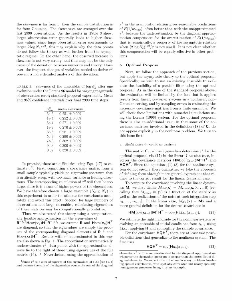
with the standard proposal, we run the EnKF with a lo-calization radius of 5 and a covariance inflation of 1.05on the Lorenz equations with 100 variables for 3000 se-quential observations. We fix ∆t = 0.4 and the systemnoise σsys = 0.01, and vary the observation error σ2

obs from5×10−3 to 1. In this experiment, we use the approximationQ̃ described above when calculating both τ and the exactweights. The size of the ensemble used to calculate Q̃ isNe,cov = 1000, but we take a subsample of size Ne = 100when calculating the weights themselves (and, as above,use Ne = 100 in the theoretical value (2 log(Ne))

1/2/τ.) Weapproximate sampling from the optimal proposal by sam-pling from the distribution derived for the linear, Gaussiancase given in Equation (A3), replacing all Q’s with Q̃.

The results are given in Figure 2. Clearly, the data

0 0.1 0.2 0.3 0.40

0.05

0.1

0.15

0.2

0.25

0.3

0.35

0.4

(2log(Ne))1/2/τ

E[1

/wm

ax]−

1

Optimal Proposal

full covsdiag covs

Fig. 2. Numerical estimation of (2 log(Ne))1/2/τ ver-

sus the time average and 95% confidence interval ofE[1/wmax]− 1 calculated using the optimal proposal, withapproximations as described in the text. Blue representscalculating τ from the true eigenvalues, and red representscalculations based on the diagonal entries of the matrix.The black line represents the theoretical relationship be-tween (2 log(Ne))

1/2/τ and E[1/wmax]− 1.

points do not agree with the theory as well as in the ex-periment with the standard proposal. This is likely dueto the parameter choices in this experiment. When us-ing the optimal proposal, we empirically found that weneeded to increase the time between observations in orderto satisfy the assumption that the filter is close to collapse(that is, that 2 log(Ne)/τ

2 is close to 0.) However, as men-tioned previously, this also leads to a steep spectrum of

8

the covariance matrices, which in turn leads to violationof the assumption that log w̃i

k is approximately Gaussian.We again investigate the values of skewness for this exper-iment; these results are given in Table 4. Note that thelonger observation time window in the optimal proposalexperiment here leads to higher values of skewness thanfor the shorter time window standard proposal experimentin the previous section.

Table 4. Skewness of the ensembles of log w̃ik after one

evolution under the Lorenz 96 model for varying magnitudeof observation error; optimal proposal experiment. Meanand 95% confidence intervals over final 2990 time steps.

σ2obs mean skewness

5e-3 0.423± 0.0100.01 0.485± 0.0110.05 0.706± 0.0140.1 0.781± 0.0160.3 0.791± 0.0160.5 0.718± 0.0141 0.577± 0.013

Thus, we would expect worse agreement with the asymp-totics in the optimal proposal experiments, because log w̃i

k

is less Gaussian than in the standard proposal experiments.The data points for which the full covariances were used (inblue) fall almost entirely above the theoretical line in solidblack. On the other hand, since approximating the eigen-values by the diagonal elements leads to underestimatingτ , the data points for which this approximation was used(in red) are much closer to the theoretical line. That is,the underestimation of τ by the diagonal approximationcompensates for the overestimation of τ by the theory dueto the steep spectrum. But, as in the case of the stan-dard proposal, these approximations are more accurate inthe asymptotic regime (close to the origin) while the datadeviates from the theory away from this regime.

6. Performance of Standard and Optimal Propos-als

Recently, there has been a focus in the particle filter-ing community on the optimal proposal as an improve-ment over the standard proposal (Doucet et al. 2000; Aru-lampalam et al. 2002; Bocquet et al. 2010; Snyder 2012;Snyder and Bengtsson 2015). Intuitively, sampling froma distribution conditioned on the new observations shouldperform better than a distribution conditioned on the pre-vious observations. The form of the weight update shouldalso provide intuition behind the performance gain: thestandard proposal weight update involves the distributionof the observations conditioned on the state at the cur-

rent time p(yk|xk), whereas the optimal proposal weightupdate is conditioned on the state at the previous time:p(yk|xk−1). Since uncertainty generally increases with alonger prediction window, the likelihood p(yk|xk−1) willtend to be broader than p(yk|xk), and thus there will beless variance across the weights for the optimal proposalupdate.

In a review of non-Gaussian data assimilation methods,Bocquet et al. (2010) performed a simple comparison be-tween the standard and optimal proposal implementationof the particle filter and found that the optimal proposalresults in lower mean squared errors for smaller ensem-ble sizes, and has comparable performance to the standardproposal for large ensemble sizes. Here, we perform exper-iments which not only compare the mean squared errors ofthese methods, but we also consider the frequency at whichresampling occurs as well as the maximum weight of eachmethod after a single step.

To test the usefulness of the optimal proposal, experi-ments were run with the Lorenz (1996) system with 5, 10,and 20 variables, with full observations once per time stepfor 300 time steps, using both the standard and optimalproposal distributions. The observation error variance, sys-tem noise variance, and initial ensemble variance are fixedat σ2

obs = 0.5, σ2sys = 0.01, σ2

ens = 1.0, respectively. Wetest two resampling thresholds: first, when the effectivesample size falls below 0.1Ne; and second, when the maxi-mum weight exceeds 0.5. After resampling, the weights arereset to 1/Ne and a small amount of jitter (with variance0.01) is added to each particle. The errors are averagedover the last 200 time steps, but the resample counts areover the entire 300-step window.

Table 5. Number of times each method resampled in awindow of 300 assimilation steps, for varying ensemble sizesand state dimensions. Top: resample when effective sam-ple size (Neff) falls below 0.1Ne. Bottom: resample whenmaximum weight (wmax) exceeds 0.5.

Ne Nx = 5 Nx = 5 Nx = 10 Nx = 10 Nx = 20 Nx = 20(Neff) std opt std opt std opt

20 254 81 297 150 298 23750 264 103 299 190 299 272100 269 113 299 195 299 277500 266 115 299 208 299 2891000 276 127 299 209 299 287

(wmax)20 272 112 297 197 297 19750 239 85 297 154 297 154100 202 76 291 129 291 129500 127 49 284 98 284 981000 125 41 265 89 265 89

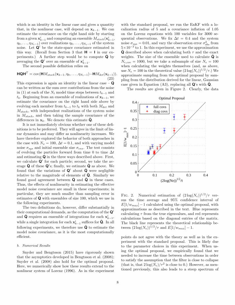
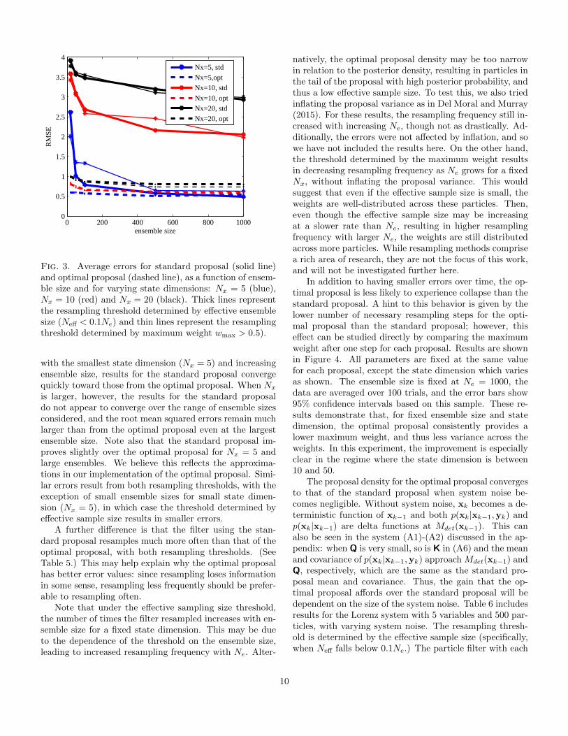
Figure 3 shows the root mean squared error of the pos-terior mean as a function of ensemble size. For the system

9

0 200 400 600 800 10000

0.5

1

1.5

2

2.5

3

3.5

4

ensemble size

RM

SE

Nx=5, std

Nx=5,opt

Nx=10, std

Nx=10, opt

Nx=20, std

Nx=20, opt

Fig. 3. Average errors for standard proposal (solid line)and optimal proposal (dashed line), as a function of ensem-ble size and for varying state dimensions: Nx = 5 (blue),Nx = 10 (red) and Nx = 20 (black). Thick lines representthe resampling threshold determined by effective ensemblesize (Neff < 0.1Ne) and thin lines represent the resamplingthreshold determined by maximum weight wmax > 0.5).

with the smallest state dimension (Nx = 5) and increasingensemble size, results for the standard proposal convergequickly toward those from the optimal proposal. When Nx

is larger, however, the results for the standard proposaldo not appear to converge over the range of ensemble sizesconsidered, and the root mean squared errors remain muchlarger than from the optimal proposal even at the largestensemble size. Note also that the standard proposal im-proves slightly over the optimal proposal for Nx = 5 andlarge ensembles. We believe this reflects the approxima-tions in our implementation of the optimal proposal. Simi-lar errors result from both resampling thresholds, with theexception of small ensemble sizes for small state dimen-sion (Nx = 5), in which case the threshold determined byeffective sample size results in smaller errors.

A further difference is that the filter using the stan-dard proposal resamples much more often than that of theoptimal proposal, with both resampling thresholds. (SeeTable 5.) This may help explain why the optimal proposalhas better error values: since resampling loses informationin some sense, resampling less frequently should be prefer-able to resampling often.

Note that under the effective sampling size threshold,the number of times the filter resampled increases with en-semble size for a fixed state dimension. This may be dueto the dependence of the threshold on the ensemble size,leading to increased resampling frequency with Ne. Alter-

natively, the optimal proposal density may be too narrowin relation to the posterior density, resulting in particles inthe tail of the proposal with high posterior probability, andthus a low effective sample size. To test this, we also triedinflating the proposal variance as in Del Moral and Murray(2015). For these results, the resampling frequency still in-creased with increasing Ne, though not as drastically. Ad-ditionally, the errors were not affected by inflation, and sowe have not included the results here. On the other hand,the threshold determined by the maximum weight resultsin decreasing resampling frequency as Ne grows for a fixedNx, without inflating the proposal variance. This wouldsuggest that even if the effective sample size is small, theweights are well-distributed across these particles. Then,even though the effective sample size may be increasingat a slower rate than Ne, resulting in higher resamplingfrequency with larger Ne, the weights are still distributedacross more particles. While resampling methods comprisea rich area of research, they are not the focus of this work,and will not be investigated further here.

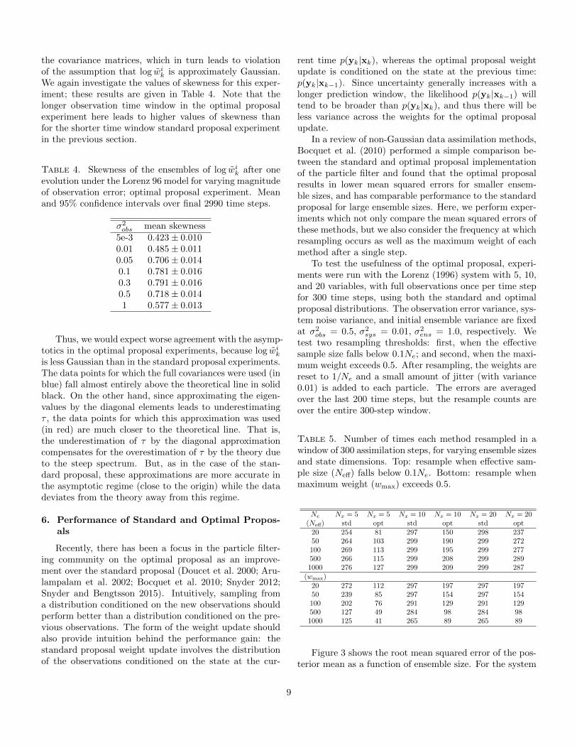
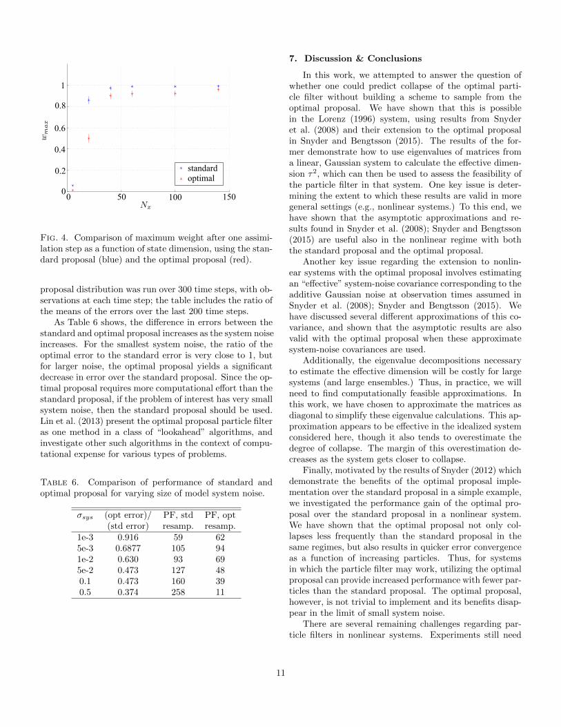
In addition to having smaller errors over time, the op-timal proposal is less likely to experience collapse than thestandard proposal. A hint to this behavior is given by thelower number of necessary resampling steps for the opti-mal proposal than the standard proposal; however, thiseffect can be studied directly by comparing the maximumweight after one step for each proposal. Results are shownin Figure 4. All parameters are fixed at the same valuefor each proposal, except the state dimension which variesas shown. The ensemble size is fixed at Ne = 1000, thedata are averaged over 100 trials, and the error bars show95% confidence intervals based on this sample. These re-sults demonstrate that, for fixed ensemble size and statedimension, the optimal proposal consistently provides alower maximum weight, and thus less variance across theweights. In this experiment, the improvement is especiallyclear in the regime where the state dimension is between10 and 50.

The proposal density for the optimal proposal convergesto that of the standard proposal when system noise be-comes negligible. Without system noise, xk becomes a de-terministic function of xk−1 and both p(xk|xk−1,yk) andp(xk|xk−1) are delta functions at Mdet(xk−1). This canalso be seen in the system (A1)-(A2) discussed in the ap-pendix: when Q is very small, so is K in (A6) and the meanand covariance of p(xk|xk−1,yk) approach Mdet(xk−1) andQ, respectively, which are the same as the standard pro-posal mean and covariance. Thus, the gain that the op-timal proposal affords over the standard proposal will bedependent on the size of the system noise. Table 6 includesresults for the Lorenz system with 5 variables and 500 par-ticles, with varying system noise. The resampling thresh-old is determined by the effective sample size (specifically,when Neff falls below 0.1Ne.) The particle filter with each

10

!

0 50 100 1500

0.2

0.4

0.6

0.8

1

standardoptimal

Fig. 4. Comparison of maximum weight after one assimi-lation step as a function of state dimension, using the stan-dard proposal (blue) and the optimal proposal (red).

proposal distribution was run over 300 time steps, with ob-servations at each time step; the table includes the ratio ofthe means of the errors over the last 200 time steps.

As Table 6 shows, the difference in errors between thestandard and optimal proposal increases as the system noiseincreases. For the smallest system noise, the ratio of theoptimal error to the standard error is very close to 1, butfor larger noise, the optimal proposal yields a significantdecrease in error over the standard proposal. Since the op-timal proposal requires more computational effort than thestandard proposal, if the problem of interest has very smallsystem noise, then the standard proposal should be used.Lin et al. (2013) present the optimal proposal particle filteras one method in a class of “lookahead” algorithms, andinvestigate other such algorithms in the context of compu-tational expense for various types of problems.

Table 6. Comparison of performance of standard andoptimal proposal for varying size of model system noise.

σsys (opt error)/ PF, std PF, opt(std error) resamp. resamp.

1e-3 0.916 59 625e-3 0.6877 105 941e-2 0.630 93 695e-2 0.473 127 480.1 0.473 160 390.5 0.374 258 11

7. Discussion & Conclusions

In this work, we attempted to answer the question ofwhether one could predict collapse of the optimal parti-cle filter without building a scheme to sample from theoptimal proposal. We have shown that this is possiblein the Lorenz (1996) system, using results from Snyderet al. (2008) and their extension to the optimal proposalin Snyder and Bengtsson (2015). The results of the for-mer demonstrate how to use eigenvalues of matrices froma linear, Gaussian system to calculate the effective dimen-sion τ2, which can then be used to assess the feasibility ofthe particle filter in that system. One key issue is deter-mining the extent to which these results are valid in moregeneral settings (e.g., nonlinear systems.) To this end, wehave shown that the asymptotic approximations and re-sults found in Snyder et al. (2008); Snyder and Bengtsson(2015) are useful also in the nonlinear regime with boththe standard proposal and the optimal proposal.

Another key issue regarding the extension to nonlin-ear systems with the optimal proposal involves estimatingan “effective” system-noise covariance corresponding to theadditive Gaussian noise at observation times assumed inSnyder et al. (2008); Snyder and Bengtsson (2015). Wehave discussed several different approximations of this co-variance, and shown that the asymptotic results are alsovalid with the optimal proposal when these approximatesystem-noise covariances are used.

Additionally, the eigenvalue decompositions necessaryto estimate the effective dimension will be costly for largesystems (and large ensembles.) Thus, in practice, we willneed to find computationally feasible approximations. Inthis work, we have chosen to approximate the matrices asdiagonal to simplify these eigenvalue calculations. This ap-proximation appears to be effective in the idealized systemconsidered here, though it also tends to overestimate thedegree of collapse. The margin of this overestimation de-creases as the system gets closer to collapse.

Finally, motivated by the results of Snyder (2012) whichdemonstrate the benefits of the optimal proposal imple-mentation over the standard proposal in a simple example,we investigated the performance gain of the optimal pro-posal over the standard proposal in a nonlinear system.We have shown that the optimal proposal not only col-lapses less frequently than the standard proposal in thesame regimes, but also results in quicker error convergenceas a function of increasing particles. Thus, for systemsin which the particle filter may work, utilizing the optimalproposal can provide increased performance with fewer par-ticles than the standard proposal. The optimal proposal,however, is not trivial to implement and its benefits disap-pear in the limit of small system noise.

There are several remaining challenges regarding par-ticle filters in nonlinear systems. Experiments still need

11

to be done to determine how the filters behave when ap-plied sequentially; all the experiments in this paper studythe degree of collapse after one assimilation step. However,this does not preclude the possibility of the particle filtercollapsing after two or more steps. In addition, it could beuseful to know whether the numerical results in this paperhave an analytical analogue, as in the linear Gaussian case.Finally, further work should be done to investigate the op-timal proposal, particularly in regards to approximationsof the model noise covariance.

Acknowledgments.

Slivinski was supported by the NSF through grantsDMS-0907904 and DMS-1148284, and by NCAR’s AdvancedStudy Program during a collaborative visit to NCAR.

APPENDIX

Sampling from Optimal Proposal

Recall that the optimal proposal requires conditioningon the current observation: p(xk|xk−1,yk) (Doucet et al.2000; Snyder 2012). Consider the case of additive Gaussiannoise and a linear observation operator, where the systemis given by

xk = M(xk−1) + ηk, (A1)

yk = Hxk + εk (A2)

with ηk ∼ N (0,Q) and εk ∼ N (0,R). Then

xk|xk−1,yk ∼ N (x̄k,P), (A3)

x̄k = (I − KH)M(xk−1) + Kyk, (A4)

P = (I − KH)Q, (A5)

K = QHT (HQHT + R)−1. (A6)

In this case, the weights have an analytic update expres-sion, since

yk|xk−1 ∼ N (HM(xk−1),HQHT + R). (A7)

Thus, the particles at time tk are first sampled from (A3),and then their weights are updated according to

wik ∝ exp

{−1

2J(xi

k−1,yk)

}wi

k−1, (A8)

J(xik−1,yk) =

(yk −HM(xi

k−1))T · (A9)(

HQHT + R)−1 (

yk −HM(xik−1)

).

REFERENCES

Ades, M. and P. van Leeuwen, 2013: An exploration of theequivalent weights particle filter. Quarterly Journal ofthe Royal Meteorological Society, 139 (672), 820–840.

Anderson, J. and S. Anderson, 1999: A Monte Carlo imple-mentation of the nonlinear filtering problem to produceensemble assimilations and forecasts. Mon. Wea. Rev.,127 (12), 2741–2758.

Arulampalam, M., S. Maskell, N. Gordon, and T. Clapp,2002: A tutorial on particle filters for onlinenonlinear/non-Gaussian Bayesian tracking. IEEE Trans-actions on Signal Processing, 50 (2), 174–188.

Bengtsson, T., P. Bickel, and B. Li, 2008: Curse of dimen-sionality revisted: Collapse of the particle filter in verylarge scale systems. Probability and Statistics: Essays inHonor of David A. Freedman, 2, 316–334, D. Nolan andT. Speed, Eds., Institute of Mathematical Statistics.

Bickel, P., B. Li, and T. Bengtsson, 2008: Sharp failurerates for the bootstrap particle filter in high dimensions.Pushing the Limits of Contemporary Statistics: Contri-butions in Honor of Jayanta K. Ghosh, 3, 318–329, b.Clarke and S. Ghosal Eds., Institute of MathematicalStatistics.

Bocquet, M., C. A. Pires, and L. Wu, 2010: Beyond Gaus-sian statistical modeling in geophysical data assimila-tion. Mon. Wea. Rev., 138 (8), 29973023.

Burgers, G., P. van Leeuwen, and G. Evensen, 1998: Anal-ysis scheme in the ensemble Kalman filter. MonthlyWeather Review, 126, 1719–1724.

Chorin, A. J. and M. Morzfeld, 2013: Conditions forsuccessful data assimilation. J. Geophys. Res. Atmos.,118 (20), 11,522–11,533, doi:10.1002/2013JD019838.

Del Moral, P. and L. Murray, 2015: Sequential Monte Carlowith highly informative observations. (in prep.).

Doucet, A., N. de Freitas, and N. Gordon, 2001: An intro-duction to sequential Monte Carlo methods. SequentialMonte Carlo Methods in Practice, 2–14, A. Doucet, N.de Freitas, and N. Gordon, Eds., Springer-Verlag.

Doucet, A., S. Godsill, and C. Andrieu, 2000: On sequen-tial Monte Carlo sampling methods for Bayesian filter-ing. Statist. Comput., 10, 197–208.

Evensen, G., 1994: Sequential data assimilation with anonlinear quasi-geostrophic model using Monte Carlomethods to forecast error statistics. J. Geophys. Res.:Oceans, 99 (C5), 10 143–10 162.

Evensen, G., 2003: The ensemble Kalman filter: theoreti-cal formulation and practical implementation. Ocean Dy-namics, 53, 343–367.

12

Gaspari, G. and S. E. Cohn, 1999: Construction of corre-lation functions in two and three dimensions. QuarterlyJournal of the Royal Meteorological Society, 125 (554),723–757.

Gordon, N., D. Salmond, and A. Smith, 1993: Novel ap-proach to nonlinear-non-Gaussian Bayesian state estima-tion. IEE Proceedings F (Radar and Signal Processing),140 (2), 107–113.

Hamill, T. M., J. S. Whitaker, and C. Snyder, 2001:Distance-dependent filtering of background error covari-ance estimates in an ensemble Kalman filter. MonthlyWeather Review, 129 (11), 2776–2790.

Hastings, W. K., 1970: Monte Carlo sampling methodsusing Markov Chains and their applications. Biometrika,57, 97–109.

Houtekamer, P. L. and H. L. Mitchell, 1998: Data assimila-tion using an ensemble Kalman filter technique. MonthlyWeather Review, 126, 796–811.

Houtekamer, P. L. and H. L. Mitchell, 2001: A sequentialensemble Kalman filter for atmospheric data assimila-tion. Monthly Weather Review, 129, 123–137.

Kong, A., J. Liu, and W. Wong, 1994: Sequential impu-tations and Bayesian missing data problems. Journal ofthe American Statistical Association, 89, 278–288.

Lin, M., R. Chen, and J. Liu, 2013: Lookahead strategiesor sequential Monte Carlo. Statistical Science, 28 (1),69–94.

Lorenz, E. N., 1996: Predictability: A problem partlysolved. Proc. Seminar on Predictability, 1, 1–18, Read-ing, Berkshire, United Kingdom, ECMWF.

Morzfeld, M., X. Tu, E. Atkins, and A. J. Chorin, 2012: Arandom map implementation of implicit filters. Journalof Computational Physics, 231 (4), 2049–2066, doi:10.1016/j.jcp.2011.11.022.

Nakano, S., G. Ueno, and T. Higuchi, 2007: Merging par-ticle filter for sequential data assimilation. Nonlin. Pro-cesses Geophys., 14 (4), 395–408.

Robert, C. P. and G. Casella, 2004: Monte-Carlo StatisticalMethods. Springer-Verlag, New York.

Silverman, B., 1986: Density estimation for statistics anddata analysis, Vol. 26. CRC press.

Snyder, C., 2012: Particle filters, the “optimal” proposaland high-dimensional systems. ECMWF Seminar onData Assimilation for Atmosphere and Ocean, Shinfield,UK, 161–170.

Snyder, C. and T. Bengtsson, 2015: Performance boundsfor particle filters using the optimal proposal. (in prep.).

Snyder, C., T. Bengtsson, P. Bickel, and J. Anderson, 2008:Obstacles to high-dimensional particle filtering. MonthlyWeather Review, 136, 4629–4640.

van Leeuwen, P., 2009: Particle filtering in geophysical sys-tems. Monthly Weather Review, 137, 4089–4114.

13