Embed Size (px)
Citation preview
GEO
MA
R R
EP
OR
T
Results from the BMBF funded project UDEMM “Umweltmonitoring für die Delaboration von Munition im Meer”
Version 1.1
Berichte aus dem GEOMAR Helmholtz-Zentrum für Ozeanforschung Kiel
Nr. 54 (N. Ser.)December 2019
Practical Guide for Environmental Monitoring
of Conventional Munitions in the Seas

Results from the BMBF funded project UDEMM “Umweltmonitoring für die Delaboration von Munition im Meer”
Version 1.1
Berichte aus dem GEOMAR Helmholtz-Zentrum für Ozeanforschung Kiel
Nr. 54 (N. Ser.)December 2019
Practical Guide for Environmental Monitoring
of Conventional Munitions in the Seas
Das GEOMAR Helmholtz-Zentrum für Ozeanforschung Kielist Mitglied der Helmholtz-Gemeinschaft
Deutscher Forschungszentren e.V.
Herausgeber / Editor:Jens Greinert
GEOMAR ReportISSN Nr.. 2193-8113, DOI 10.3289/GEOMAR_REP_NS_54_2019
Helmholtz-Zentrum für Ozeanforschung Kiel / Helmholtz Centre for Ocean Research KielGEOMARDienstgebäude Westufer / West Shore BuildingDüsternbrooker Weg 20D-24105 KielGermany
Helmholtz-Zentrum für Ozeanforschung Kiel / Helmholtz Centre for Ocean Research KielGEOMARDienstgebäude Ostufer / East Shore BuildingWischhofstr. 1-3D-24148 KielGermany
Tel.: +49 431 600-0Fax: +49 431 600-2805www.geomar.de
The GEOMAR Helmholtz Centre for Ocean Research Kielis a member of the Helmholtz Association of
German Research Centres
Practical Guide for
Environmental Monitoring of Conventional
Munitions in the Seas Results from the BMBF funded project UDEMM
“Umweltmonitoring für die Delaboration von Munition im Meer“
Version 1.1
Version / Date Contribution Contributor
26 April 2019 First outline draft UDEMM partners; GEOMAR, CAU, IOW
5 September 2019 First distributed draft V1.1 UDEMM partners; GEOMAR, CAU, IOW, BLANO, EGEOS
16 September 2019 Added: Biota analyses in section 2.3 GEOMAR
5 November 2019 Added knowledge gaps chapter GEOMAR
5 December 2019 Final editing for Version 1.1 GEOMAR
Editor: Jens Greinert - GEOMAR
With contributions from: Daniel Appel, Aaron Beck, Anja Eggert, Ulf Gräwe, Mareike Kampmeier, Hans-Jörg
Martin, Edmund Maser, Christian Schlosser, Yifan Song, Jennifer Strehse, Eefke van der Lee, Rahel Vortmeyer-Kley,
Uwe Wichert, Torsten Frey
Financial support was given by: BMBF project UDEMM (grants 03F0747A, B, C); at GEOMAR additionally through
in-house funds; at CAU additionally through MATEP as part of the Cluster of Excellence ‘Future Ocean’; WT.SH
funding 123 16 006-UKSH and support from MELUND.
UDEMM Practical Guide for Environmental Monitoring of Conventional Munition in the Seas V1.1 December 2019
1
Contents Preface .......................................................................................................................................................... 2
1. Conventional munitions in the sea: Threats and problems ...................................................................... 4
1.1 What are the threats? ......................................................................................................................... 4
1.2 What are the methodological tasks and problems? ........................................................................... 7
1.3 Further information and related regulations .................................................................................... 12
2. Case study Kolberger Heide and western German Baltic Sea ................................................................. 15
2.1 History of the study area Kolberger Heide ....................................................................................... 16
2.2 Hydro-acoustic and visual mapping results ...................................................................................... 18
2.3 Munitions compounds in water, sediment and biota ...................................................................... 20
2.4 Bio-Monitoring .................................................................................................................................. 32
2.5 Oceanographic field measurements ................................................................................................. 38
2.6 Coupled TNT-GETM model................................................................................................................ 40
2.7 Conclusion, knowledge gaps and recommendations ....................................................................... 46
2.7.1 In Conclusion .............................................................................................................................. 46
2.7.2 Knowledge gaps ......................................................................................................................... 47
2.7.3 Recommendation ....................................................................................................................... 49
3. Practical guidence for sampling and monitoring .................................................................................... 51
3.1 Scientifically “best” monitoring ........................................................................................................ 51
3.2 Baseline Study ................................................................................................................................... 52
3.3 Long-term monitoring ....................................................................................................................... 56
3.4 Monitoring during clearance activities ............................................................................................. 60
4. Methodologies ........................................................................................................................................ 62
4.0 Historical Analysis ............................................................................................................................. 62
4.1 Acoustic mapping and monitoring .................................................................................................... 63
4.2 Visual observations and mapping ..................................................................................................... 68
4.3 Field sampling of sediment and biota ............................................................................................... 72
4.4 Habitat mapping ............................................................................................................................... 72
4.5 Oceanographic monitoring ............................................................................................................... 73
4.6 Modelling of currents, TNT distribution including its bio-degradation ............................................ 74
4.7 Water sampling ................................................................................................................................. 77
4.8 Bio-Monitoring with mussels ............................................................................................................ 79
4.9 Chemical analyses of water, sediment and organic matter.............................................................. 81
4.9.1 Sample preparation ................................................................................................................... 81
4.9.2 Analysis ...................................................................................................................................... 82
5. Appendix ................................................................................................................................................. 84
5.1 Analysis of nitroaromatic compounds in mussel tissue (blue mussels) ............................................ 84

UDEMM Practical Guide for Environmental Monitoring of Conventional Munition in the Seas V1.1 December 2019
2
Preface This “Practical Guide for Environmental Monitoring of Conventional Munitions in the Sea” has been
developed as part of the joint scientific project UDEMM (March 2016 - June 2019) funded by the Federal
Ministry of Education and Research Germany with partners from GEOMAR Helmholtz-Centre for Ocean
Research Kiel (GEOMAR), the Christian-Albrechts University in Kiel (CAU) and the Baltic Sea Research
Institute in Warnemünde (IOW). Four research groups combined their expertise to test and develop new
methodologies, develop a monitoring strategy and investigate the current environmental state of a
munitions dumping ground. The detailed objectives were to:
• better understand the current state of munitions contamination in the munitions dumping
ground at Kolberger Heide
• apply or newly develop state-of-the-art monitoring technologies for:
a) highly detailed mapping of munitions on the seafloor with hydroacoustic and optical
means
b) the chemical analyses of munitions contaminants in water and sediments
c) the uptake of munitions contaminants into organisms and the establishment of toxic
thresholds
• setup and advance an existing oceanographic model of the Baltic Sea to extrapolate the
distribution of munitions contamination
• verify the validity of assumptions and modelling during sampling campaigns in Kiel Bay and the
entire German Baltic Sea
Four research groups worked on these objectives. The group of Prof. Greinert (GEOMAR) applied
multibeam mapping technologies, visual investigations by towed camera, autonomous underwater
vehicles (AUV) and divers as well as sediment sampling to map and classify munition and the specific
habitat within the different study areas. These maps served as base information to guide water sampling
and in-situ experiments for TNT dissolution rates that were undertaken by the group of Prof.
Achterberg (GEOMAR). A second focus of Achterberg’s group was to establish a workflow and analytical
technologies for measuring munitions compounds (MC) in water samples with very low detection limits
on the order of fg/L (10-15g/L). In parallel the group of Prof. Maser (CAU) aimed at using mussels for
biomonitoring of munitions contaminants Analytical advancements and toxicological interpretation of
data were part of the group’s work. Finally the group of Dr. Graewe (IOW) used the existing Baltic Sea
Model (GETM; General Estuarine Transport Model) and implemented chemical and biological modules
for the dissolution and turnover of explosive compounds in dependence of seasonally changing current
and temperature conditions.
For logistic reasons, the area marked as explosives dumping ground (disused) located in the marine area
Kolberger Heide, just off Schönberg (Plön County, Schleswig-Holstein (SH)) was selected as the main
study area. This shallow area (7-19m water depth), only 12 nautical miles (nmi) from Kiel, was the ideal
location for such scientific studies, easy to reach with GEOMAR vessels and shallow enough for divers
and with reasonably good visibility due to the sandy sediment. From the very beginning it was clear that
UDEMM Practical Guide for Environmental Monitoring of Conventional Munition in the Seas V1.1 December 2019
3
an integrated approach of geologists/geophysicists, chemists, toxicologists and physical oceanographers
was needed to acquire and generate scientifically valid data to fulfil the objectives mentioned above.
The aim of this Practical Guide is to summarize the results of the UDEMM project, give an evaluation of
the state of contamination in the Kolberger Heide, introduce the use of commonly available and newly
developed technologies and present a blueprint for monitoring efforts with regards to the
“Environmental Monitoring of Conventional Munitions in the Sea”. Some, but not all of the presented
results have been published in peer reviewed scientific journals. Several assumptions are presented
although a final and scientifically sound proof cannot be given; this is because long-term monitoring still
needs to be performed before conclusions can be drawn.
This guide is a living document, which we aim to update in the coming years as part of new projects and
in-house investigations. Thus it should not be seen as a final product but rather as a work in progress.
Nevertheless, we believe that substantial progress has been made in developing a monitoring strategy
and the necessary technologies, and that these are now accessible to scientists, governmental bodies,
NGOs, and companies who are asked to implement such monitoring activities.

UDEMM Practical Guide for Environmental Monitoring of Conventional Munition in the Seas V1.1 December 2019
4
1. Conventional munitions in the sea: Threats and
problems
1.1 What are the threats? Several threats exist with regards to munitions in the sea. The most important one today in Germany –
and many other countries – is the risk of explosions during underwater construction work. In Germany
the establishment of offshore wind-parks for power generation brought the problem of munitions in the
sea again to the attention of politicians and the public. Secondly, findings of munitions along beaches
and related accidents with munitions washed onshore, including findings of white phosphorous,
highlight that munitions dumped after WWI and WWII are not ‘safely stored away’ but constitutes a
constant threat that impacts beach visitors. Other threats exist, which are presented in Table 1; the risk
levels assigned to these threats are how the UDEMM consortium sees them without claiming that
scientifically valid data have been acquired as a basis of this assessment. Our assessment is mainly based
on own experience and measurements in the field, through discussions with colleagues from other
countries, as well as with authorities in Germany as there are: Ministry of Energy, Agriculture, the
Environment, Nature and Digitalization in SH (MELUND), and the German Navy, the
Kampfmittelräumdienst – Explosive Ordnance Disposal (EOD) service in SH, the German Federal
Maritime and Hydrographic Agency (BSH). A thorough risk assessment was not possible as methods and
workflows to generate the necessary data were not available at the beginning of the UDEMM project.
Only after thorough monitoring efforts have been conducted, a reliable risk assessment can be made.
This Practical Guide shows how we, the UDEMM consortium, think such monitoring can/should be done.
Table 1: Current threats as seen by the UDEMM consortium; see more details here1.
Threats Risks in the Baltic Sea (regional to coastal scale)
Risks in Kiel Bay (local scale)
Marine Traffic
Ships run on ground Low: No reports of such instances; state of technology and safety features in ships is high.
Low: No reports of such instances; state of technology and safety features in ships is high.
Construction
General construction
Medium: Offshore wind parks are installed in the Baltic and other Seas. Thorough mapping and clearance of construction sites needs to be done prior constructions.
Low: Currently no large constructions planned in Kiel Bay, however thorough mapping and clearance of local construction sites needs to be done prior constructions.
Dredging
Medium: Most of the area. Very high: Spatially threats increase, thorough mapping, clearance or other precautionary measures strongly recommended.
Low: With the exceptions of central Hohwachter Bucht and some other restricted areas indicated in official sea charts.
Coastal protection Medium: Most of the area. Very high: Spatially threats increase, thorough mapping, clearance or other
Low: With exceptions of small sections of beaches known to be contaminated with warfare material.
1 Only in German: https://www.schleswig-holstein.de/DE/UXO/Berichte/PDF/Berichte/aa_blmp_langbericht.pdf
UDEMM Practical Guide for Environmental Monitoring of Conventional Munition in the Seas V1.1 December 2019
5
precautionary measures strongly recommended.
Public & recreational activities
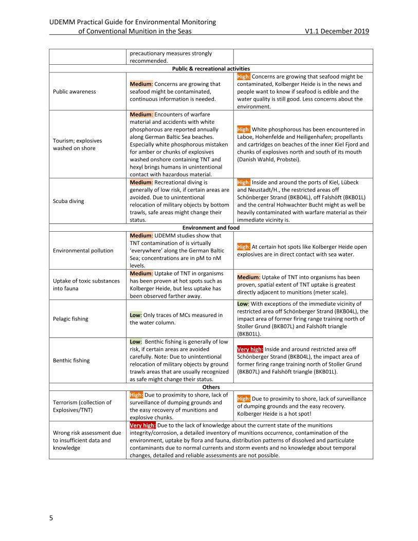
Public awareness Medium: Concerns are growing that seafood might be contaminated, continuous information is needed.
High: Concerns are growing that seafood might be contaminated, Kolberger Heide is in the news and people want to know if seafood is edible and the water quality is still good. Less concerns about the environment.
Tourism; explosives washed on shore
Medium: Encounters of warfare material and accidents with white phosphorous are reported annually along German Baltic Sea beaches. Especially white phosphorous mistaken for amber or chunks of explosives washed onshore containing TNT and hexyl brings humans in unintentional contact with hazardous material.
High: White phosphorous has been encountered in Laboe, Hohenfelde and Heiligenhafen; propellants and cartridges on beaches of the inner Kiel Fjord and chunks of explosives north and south of its mouth (Danish Wahld, Probstei).
Scuba diving
Medium: Recreational diving is generally of low risk, if certain areas are avoided. Due to unintentional relocation of military objects by bottom trawls, safe areas might change their status.
High: Inside and around the ports of Kiel, Lübeck and Neustadt/H., the restricted areas off Schönberger Strand (BKB04L), off Falshöft (BKB01L) and the central Hohwachter Bucht might as well be heavily contaminated with warfare material as their immediate vicinity is.
Environment and food
Environmental pollution
Medium: UDEMM studies show that TNT contamination of is virtually ‘everywhere’ along the German Baltic Sea; concentrations are in pM to nM levels.
High: At certain hot spots like Kolberger Heide open explosives are in direct contact with sea water.
Uptake of toxic substances into fauna
Medium: Uptake of TNT in organisms has been proven at hot spots such as Kolberger Heide, but less uptake has been observed farther away.
Medium: Uptake of TNT into organisms has been proven, spatial extent of TNT uptake is greatest directly adjacent to munitions (meter scale).
Pelagic fishing Low: Only traces of MCs measured in the water column.
Low: With exceptions of the immediate vicinity of restricted area off Schönberger Strand (BKB04L), the impact area of former firing range training north of Stoller Grund (BKB07L) and Falshöft triangle (BKB01L).
Benthic fishing
Low: Benthic fishing is generally of low risk, if certain areas are avoided carefully. Note: Due to unintentional relocation of military objects by ground trawls areas that are usually recognized as safe might change their status.
Very high: Inside and around restricted area off Schönberger Strand (BKB04L), the impact area of former firing range training north of Stoller Grund (BKB07L) and Falshöft triangle (BKB01L).
Others
Terrorism (collection of Explosives/TNT)
High: Due to proximity to shore, lack of surveillance of dumping grounds and the easy recovery of munitions and explosive chunks.
High: Due to proximity to shore, lack of surveillance of dumping grounds and the easy recovery. Kolberger Heide is a hot spot!
Wrong risk assessment due to insufficient data and knowledge
Very high: Due to the lack of knowledge about the current state of the munitions integrity/corrosion, a detailed inventory of munitions occurrence, contamination of the environment, uptake by flora and fauna, distribution patterns of dissolved and particulate contaminants due to normal currents and storm events and no knowledge about temporal changes, detailed and reliable assessments are not possible.
UDEMM Practical Guide for Environmental Monitoring of Conventional Munition in the Seas V1.1 December 2019
6
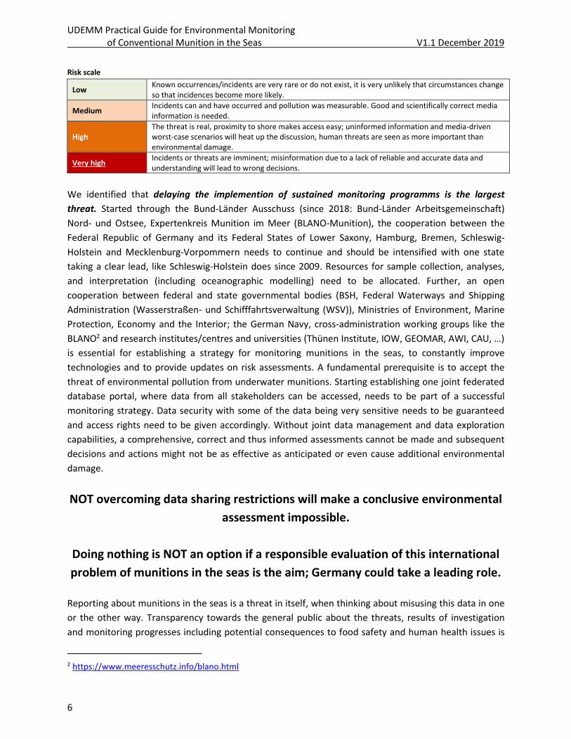
Risk scale
Low Known occurrences/incidents are very rare or do not exist, it is very unlikely that circumstances change so that incidences become more likely.
Medium Incidents can and have occurred and pollution was measurable. Good and scientifically correct media information is needed.
High The threat is real, proximity to shore makes access easy; uninformed information and media-driven worst-case scenarios will heat up the discussion, human threats are seen as more important than environmental damage.
Very high Incidents or threats are imminent; misinformation due to a lack of reliable and accurate data and understanding will lead to wrong decisions.
We identified that delaying the implemention of sustained monitoring programms is the largest
threat. Started through the Bund-Länder Ausschuss (since 2018: Bund-Länder Arbeitsgemeinschaft)
Nord- und Ostsee, Expertenkreis Munition im Meer (BLANO-Munition), the cooperation between the
Federal Republic of Germany and its Federal States of Lower Saxony, Hamburg, Bremen, Schleswig-
Holstein and Mecklenburg-Vorpommern needs to continue and should be intensified with one state
taking a clear lead, like Schleswig-Holstein does since 2009. Resources for sample collection, analyses,
and interpretation (including oceanographic modelling) need to be allocated. Further, an open
cooperation between federal and state governmental bodies (BSH, Federal Waterways and Shipping
Administration (Wasserstraßen- und Schifffahrtsverwaltung (WSV)), Ministries of Environment, Marine
Protection, Economy and the Interior; the German Navy, cross-administration working groups like the
BLANO2 and research institutes/centres and universities (Thünen Institute, IOW, GEOMAR, AWI, CAU, …)
is essential for establishing a strategy for monitoring munitions in the seas, to constantly improve
technologies and to provide updates on risk assessments. A fundamental prerequisite is to accept the
threat of environmental pollution from underwater munitions. Starting establishing one joint federated
database portal, where data from all stakeholders can be accessed, needs to be part of a successful
monitoring strategy. Data security with some of the data being very sensitive needs to be guaranteed
and access rights need to be given accordingly. Without joint data management and data exploration
capabilities, a comprehensive, correct and thus informed assessments cannot be made and subsequent
decisions and actions might not be as effective as anticipated or even cause additional environmental
damage.
NOT overcoming data sharing restrictions will make a conclusive environmental
assessment impossible.
Doing nothing is NOT an option if a responsible evaluation of this international
problem of munitions in the seas is the aim; Germany could take a leading role.
Reporting about munitions in the seas is a threat in itself, when thinking about misusing this data in one
or the other way. Transparency towards the general public about the threats, results of investigation
and monitoring progresses including potential consequences to food safety and human health issues is
2 https://www.meeresschutz.info/blano.html
UDEMM Practical Guide for Environmental Monitoring of Conventional Munition in the Seas V1.1 December 2019
7
important as this will show that the problem of munitions in the seas is taken seriously. However, to a
certain extend some information needs to be disclosed from the public; this is particularly true for
presenting exact locations of ammunition objects, exact numbers and state of corrosion. Because of this,
all detailed maps in this report do not show coordinates. Exact sample locations should not be given in
public documents, including scientific publications. UDEMM members, together with partners at the
German Navy, the BLANO and Kampfmittelräumdienst Schleswig-Holstein, agreed on publishing
coordinates with an accuracy of less than ~180 m (one digit for minute values of coordinates, e.g.
DDD°MM.m’).
1.2 What are the methodological tasks and problems? Even after overcoming financial, time, data management and responsibility issues, methodological tasks
and related problems remain, which need to be considered for a scientifically sound monitoring. Three
major tasks exist:
A. how to monitor munitions dumping grounds
B. how to define toxicity levels
C. how to evaluate the risks
This guide focuses on the first task of “how to monitor munitions dumping grounds” and gives insights
into the definition of toxicity levels. Defining risks or developing decision workflows for evaluating the
risks of munitions in the seas was not topic of UDEMM. The parallel running project DIAMON3 focused
on this task and presented a first version of a Decision Support Tool. This tool strongly depends on
reliable and conclusive data. How to acquire such data was the goal of UDEMM and to focus efforts of
such a complex task, one dumping ground type was studied in detail. Within the area of Kolberger
Heide, large ammunition objects and chunks of explosives are distributed on the seafloor surface in
relatively shallow water. For such and other scenarios the monitoring can be sorted according to five
overarching topics:
A. the occurrence/distribution of ammunition objects and their redistribution/ migration over time
B. the dissolution flux of contaminants from solid explosives into the water, and the mechanisms
and timescales of conversion into non-toxic substances
C. the spatial and temporal distribution of dissolved and particulate contaminants in the water
column
D. the uptake and accumulation of contaminants by organisms and the occurrence within the food
web
E. the consequences of munition-related contamination for specific habitats and the environment
in general
3 https://www.daimonproject.com/
UDEMM Practical Guide for Environmental Monitoring of Conventional Munition in the Seas V1.1 December 2019
8
This guide deals with topics A to D and the respective results gained through the UDEMM project;
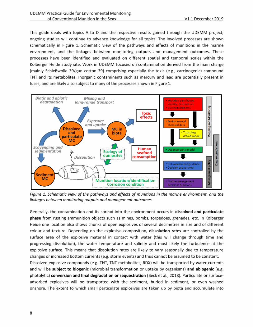
ongoing studies will continue to advance knowledge for all topics. The involved processes are shown
schematically in Figure 1. Schematic view of the pathways and effects of munitions in the marine
environment, and the linkages between monitoring outputs and management outcomes. These
processes have been identified and evaluated on different spatial and temporal scales within the
Kolberger Heide study site. Work in UDEMM focused on contamination derived from the main charge
(mainly Schießwolle 39/gun cotton 39) comprising especially the toxic (e.g., carcinogenic) compound
TNT and its metabolites. Inorganic contaminants such as mercury and lead are potentially present in
fuses, and are likely also subject to many of the processes shown in Figure 1.
Figure 1. Schematic view of the pathways and effects of munitions in the marine environment, and the linkages between monitoring outputs and management outcomes.
Generally, the contamination and its spread into the environment occurs in dissolved and particulate
phase from rusting ammunition objects such as mines, bombs, torpedoes, grenades, etc. In Kolberger
Heide one location also shows chunks of open explosives of several decimetres in size and of different
colour and texture. Depending on the explosive composition, dissolution rates are controlled by the
surface area of the explosive material in contact with water (this will change through time and
progressing dissolution), the water temperature and salinity and most likely the turbulence at the
explosive surface. This means that dissolution rates are likely to vary seasonally due to temperature
changes or increased bottom currents (e.g. storm events) and thus cannot be assumed to be constant.
Dissolved explosive compounds (e.g. TNT, TNT metabolites, RDX) will be transported by water currents
and will be subject to biogenic (microbial transformation or uptake by organisms) and abiogenic (e.g.
photolytic) conversion and final degradation or sequestration (Beck et al., 2018). Particulate or surface-
adsorbed explosives will be transported with the sediment, buried in sediment, or even washed
onshore. The extent to which small particulate explosives are taken up by biota and accumulate into
UDEMM Practical Guide for Environmental Monitoring of Conventional Munition in the Seas V1.1 December 2019
9
their tissue is still largely unknown. Rapid dissolution in the water column is likely to limit the
redistribution and impact of intact explosive particles.
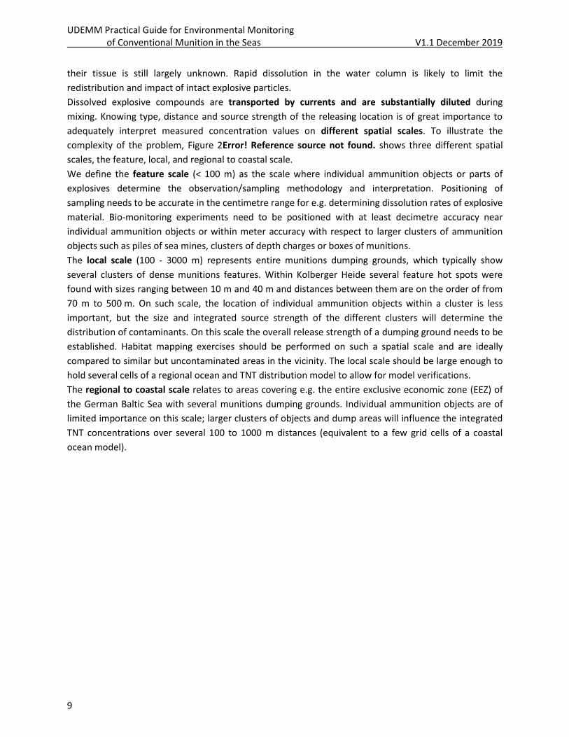
Dissolved explosive compounds are transported by currents and are substantially diluted during
mixing. Knowing type, distance and source strength of the releasing location is of great importance to
adequately interpret measured concentration values on different spatial scales. To illustrate the
complexity of the problem, Figure 2Error! Reference source not found. shows three different spatial
scales, the feature, local, and regional to coastal scale.
We define the feature scale (< 100 m) as the scale where individual ammunition objects or parts of
explosives determine the observation/sampling methodology and interpretation. Positioning of
sampling needs to be accurate in the centimetre range for e.g. determining dissolution rates of explosive
material. Bio-monitoring experiments need to be positioned with at least decimetre accuracy near
individual ammunition objects or within meter accuracy with respect to larger clusters of ammunition
objects such as piles of sea mines, clusters of depth charges or boxes of munitions.
The local scale (100 - 3000 m) represents entire munitions dumping grounds, which typically show
several clusters of dense munitions features. Within Kolberger Heide several feature hot spots were
found with sizes ranging between 10 m and 40 m and distances between them are on the order of from
70 m to 500 m. On such scale, the location of individual ammunition objects within a cluster is less
important, but the size and integrated source strength of the different clusters will determine the
distribution of contaminants. On this scale the overall release strength of a dumping ground needs to be
established. Habitat mapping exercises should be performed on such a spatial scale and are ideally
compared to similar but uncontaminated areas in the vicinity. The local scale should be large enough to
hold several cells of a regional ocean and TNT distribution model to allow for model verifications.
The regional to coastal scale relates to areas covering e.g. the entire exclusive economic zone (EEZ) of
the German Baltic Sea with several munitions dumping grounds. Individual ammunition objects are of
limited importance on this scale; larger clusters of objects and dump areas will influence the integrated
TNT concentrations over several 100 to 1000 m distances (equivalent to a few grid cells of a coastal
ocean model).
UDEMM Practical Guide for Environmental Monitoring of Conventional Munition in the Seas V1.1 December 2019
10
Figure 2: Overview of the different spatial scales that need to be considered during munitions studies. A) Shows the bathymetry of an area with explosion crates and dumped munitions (ground mines and torpedo heads) in the Kolberger Heide. B) Shows the bathymetry of the Kolberger Heide with ammunition objects marked with grey dots (total 1,136). C) Germany Baltic Sea with points indicating water sampling stations during POS530 (October 2018) and munitions dumping grounds (red), munitions occurrence areas (red pattern) and munitions suspected areas (red polygons).
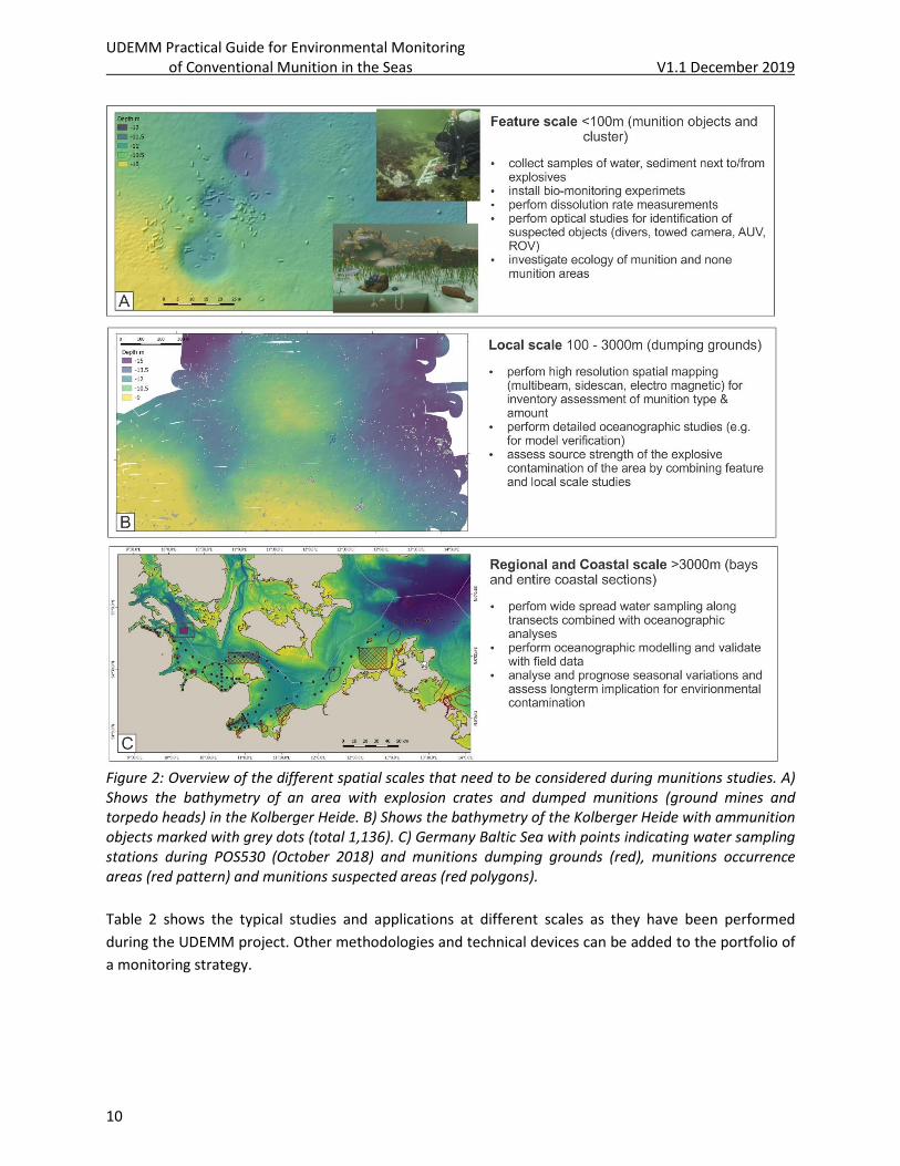
Table 2 shows the typical studies and applications at different scales as they have been performed
during the UDEMM project. Other methodologies and technical devices can be added to the portfolio of
a monitoring strategy.
UDEMM Practical Guide for Environmental Monitoring of Conventional Munition in the Seas V1.1 December 2019
11
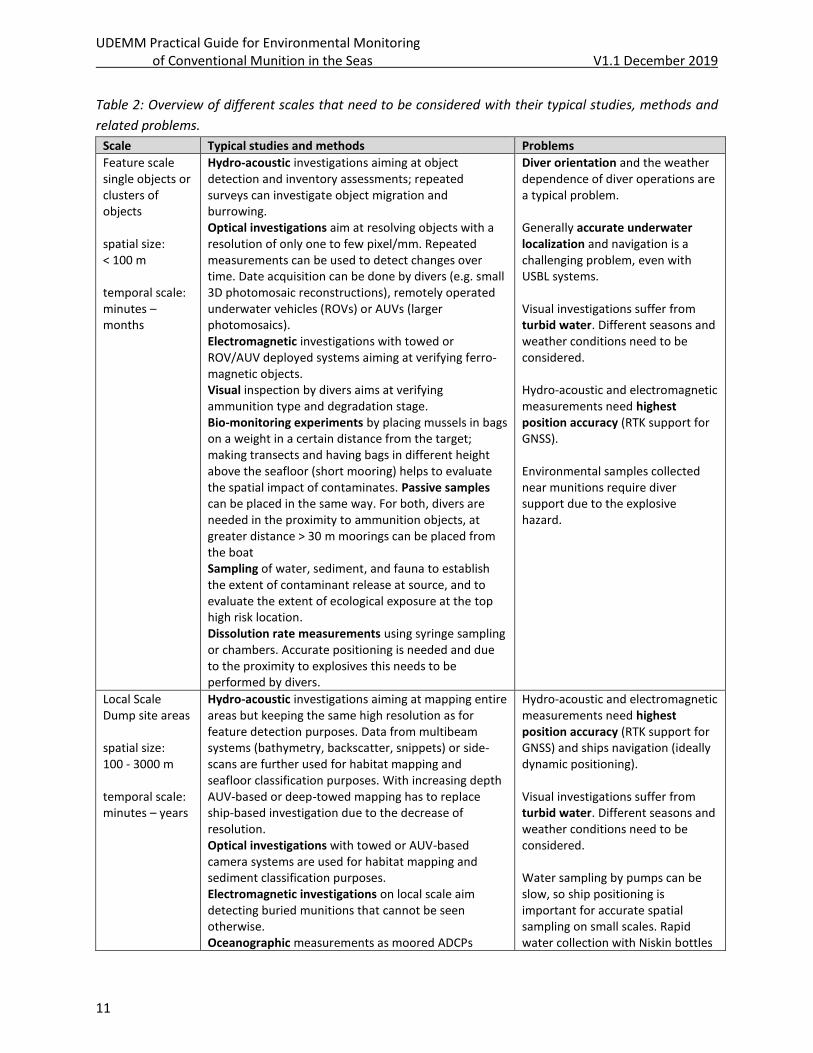
Table 2: Overview of different scales that need to be considered with their typical studies, methods and
related problems.
Scale Typical studies and methods Problems
Feature scale single objects or clusters of objects spatial size: < 100 m temporal scale: minutes – months
Hydro-acoustic investigations aiming at object detection and inventory assessments; repeated surveys can investigate object migration and burrowing. Optical investigations aim at resolving objects with a resolution of only one to few pixel/mm. Repeated measurements can be used to detect changes over time. Date acquisition can be done by divers (e.g. small 3D photomosaic reconstructions), remotely operated underwater vehicles (ROVs) or AUVs (larger photomosaics). Electromagnetic investigations with towed or ROV/AUV deployed systems aiming at verifying ferro-magnetic objects. Visual inspection by divers aims at verifying ammunition type and degradation stage. Bio-monitoring experiments by placing mussels in bags on a weight in a certain distance from the target; making transects and having bags in different height above the seafloor (short mooring) helps to evaluate the spatial impact of contaminates. Passive samples can be placed in the same way. For both, divers are needed in the proximity to ammunition objects, at greater distance > 30 m moorings can be placed from the boat Sampling of water, sediment, and fauna to establish the extent of contaminant release at source, and to evaluate the extent of ecological exposure at the top high risk location. Dissolution rate measurements using syringe sampling or chambers. Accurate positioning is needed and due to the proximity to explosives this needs to be performed by divers.
Diver orientation and the weather dependence of diver operations are a typical problem. Generally accurate underwater localization and navigation is a challenging problem, even with USBL systems. Visual investigations suffer from turbid water. Different seasons and weather conditions need to be considered. Hydro-acoustic and electromagnetic measurements need highest position accuracy (RTK support for GNSS). Environmental samples collected near munitions require diver support due to the explosive hazard.
Local Scale Dump site areas spatial size: 100 - 3000 m temporal scale: minutes – years
Hydro-acoustic investigations aiming at mapping entire areas but keeping the same high resolution as for feature detection purposes. Data from multibeam systems (bathymetry, backscatter, snippets) or side-scans are further used for habitat mapping and seafloor classification purposes. With increasing depth AUV-based or deep-towed mapping has to replace ship-based investigation due to the decrease of resolution. Optical investigations with towed or AUV-based camera systems are used for habitat mapping and sediment classification purposes. Electromagnetic investigations on local scale aim detecting buried munitions that cannot be seen otherwise. Oceanographic measurements as moored ADCPs
Hydro-acoustic and electromagnetic measurements need highest position accuracy (RTK support for GNSS) and ships navigation (ideally dynamic positioning). Visual investigations suffer from turbid water. Different seasons and weather conditions need to be considered. Water sampling by pumps can be slow, so ship positioning is important for accurate spatial sampling on small scales. Rapid water collection with Niskin bottles
UDEMM Practical Guide for Environmental Monitoring of Conventional Munition in the Seas V1.1 December 2019
12
(Acoustic Doppler Current Profiler) or CTDs (Conductivity Temperature Depth) record the local variability of physical parameters over longer time (months - years) in high temporal resolution. Such data are used to validate oceanographic model results and as input parameters e.g. in dissolution models. Sampling of water helps indicate the integrated local source strength, and the extent to which released contaminants are spread away from the source. Sample depths need to be adjusted to the actual stratification of the water column. Transects across and away from the dumping grounds should be considered, sample spacing can be linked to the model cell size. Sampling of sediment is needed to ground truth sediment classification (needed for munitions burial estimates), as well as for analyses of explosive compounds (evaluating the extent to which contaminants are accumulated in sediments). Biota sampling is necessary to determine the extent of ecological exposure outside the immediate contamination source, yet within the zone of elevated concentrations.
is preferred.
Regional Scale Coastal areas spatial size: > 3000 m temporal scale: days to decades
Sampling of water aims at quantifying the spread of contaminants outside of known dumping grounds. Changing distribution patterns with a focus towards sensitive areas (fishing grounds, tourist areas) will be analysed. Sample depths need to be adjusted to the actual stratification of the water column. Bio-monitoring at specific locations outside of dumping grounds will support the evaluation of contamination spread and uptake into the food web. Oceanographic modelling is to determine the integrated source strength of an area and predict spreading over time (warning system).
“Large” amount of water analyses accompanied by physical measurements are needed for gathering a comprehensive data set. With increasing knowledge and duration of monitoring, the amount of samples can most likely be reduced. Oceanographic modelling with combined ‘TNT’ dissolution and degradation modules is needed (high performance computing).
1.3 Further information and related regulations The above short introduction does not claim to be complete in its methods, it is so far the first
compilation of munitions monitoring recommendations publically available in Germany and, to our
knowledge, in Europe. Ongoing research and monitoring results will contribute to this ‘Best Practices
Guide’ and will constantly extend and improve it.
Yearly meetings of researchers, authorities and subcontractors, who execute the monitoring, shall lead
to a yearly updated version of this document, results and progress of monitoring should be introduced
and maintained under the Monitoring Handbook of BLMP4.
This is the continuation of the work and discussions, which made sure, that the topic of sea-dumped
munitions finally reached political levels. First efforts for Northern Europe started in 1974, when the
Helsinki Convention introduced first guidelines for the protection of the marine environment of the
4 https://mhb.meeresschutz.info/de/start
UDEMM Practical Guide for Environmental Monitoring of Conventional Munition in the Seas V1.1 December 2019
13
Baltic Sea area (Carton and Jagusiewicz, 2009). This led to the federation of the bordering states and the
European Economic Community, and the ratification of the HELCOM convention (‘Baltic Marine
Environment Protection Commission - Helsinki Commission’) (Carton and Jagusiewicz, 2009). With
signing the convention the parties agreed to prohibit sea-dumping of waste, including chemical and
conventional munitions (Carton and Jagusiewicz, 2009; HELCOM, 2014). Equivalently, the OSPAR (‘Oslo-
Paris Convention for the Protection of the Marine Environment of the Northeast-Atlantic’) convention
applies for the North Sea area (OSPAR Commission, 2007). In addition, the European initiative of the
Marine Strategy Framework Directive (MSFD) aims for establishing a good environmental status of
European waters by 2020. Within the directive’s descriptor 8, munitions disposal sites are explicitly
named as a source for contamination and pollution (Law et al., 20105).
To comply with the MSFD, Germany e.g. has established a monitoring program called BLMP
(Bund/Länder Messprogramm). This programme has released a public report on Munitions in German
Marine Waters - Stocktaking and Recommendations, concluding that the status of munitions within
German waters remains unknown to a large extent (Böttcher et al., 2011). Even though the report is
updated yearly, the situation in general remains the same, while an effective monitoring procedure has
not yet been established. About 300,000 metric tons of conventional munitions and 5,000 metric tons of
chemical warfare (CW) material have been brought into German waters of the Baltic Sea. The North Sea
contains around 1,300,000 metric tons of conventional and 9,000 metric tons of chemical munitions
(Böttcher et al., 2011). In addition of unexploded ordnance from combat and bombing (UXO), all kinds of
munitions from onshore munitions depots have been dumped after World War II (WWII) in dedicated
nearshore areas. Instead of shipping the munitions to the official dumping grounds, it was common
practice to start dumping along the way to the designated areas – also known as ‘on-route-dumping’
(Böttcher et al., 2011; 2015). This and the dislocations of ordnance and initial relocations by fishery
activities, make it difficult to estimate exact numbers of munitions inside those areas (Beddington and
Kinloch, 2005; Böttcher et al., 2011; 2015; 2016). If not blown in place, defused munitions have been
taken out of the water to a large extend (95 % of 21,000 objects reported since 2013) and has been
disposed on land. A small fraction though could not be taken out (i.e. British ground mines) but where
relocated by the Kampfmittelräumdienst (or EOD service – explosive ordnance disposal service) to a
marine dumping ground instead. This is also done because WWII explosives, having rested underwater
for seventy years by now, become increasingly unstable and the risk of a spontaneous detonation during
transport, particularly onshore, has strongly increased (Pfeiffer, 2012). Due to this necessary time-
consuming and costly practice, the number of ammunition objects in the sea is effectively not
decreasing so far. Nautical charts indicate certain areas of the seafloor according to IMO-Standards for
electronic nautical charts (ENS) as:
• Explosives dumping ground, individual mine or explosive (No. 23.1)
• Explosives dumping ground (disused), Foul (explosives) (No. 23.2) or
• Dumping ground for Chemical waste [including chemical waste from sea dumped chemical
munitions] (No. 24).
5 https://mcc.jrc.ec.europa.eu/documents/201801085655.pdf
UDEMM Practical Guide for Environmental Monitoring of Conventional Munition in the Seas V1.1 December 2019
14
Despite this, their precise boundary, actual amount of munitions and the extent of munitions just
outside the dumping grounds is barely known (Beddington and Kinloch, 2005; Böttcher et al, 2011 -
2018; United Nations Mine Action Service, 2014). Therefor the map published by Böttcher et al. 2011
indicated
• 15 munitions dumping grounds (dedicated areas)
• 56 munitions-contaminated areas (e.g. routes from operational ports to dumping grounds
• 21 munitions suspected areas in German territorial waters.
Due to their proximity to shore and thus densely populated areas as well as marine shipping routes, it is
urgent to gain a better picture of the state of the different munitions under water. As the problem will
not disappear but rather spread, it is necessary to establish monitoring procedures for long-term
observations and risk assessments of those dumping grounds. Here, we present results of the German
BMBF-funded project UDEMM (‘environmental monitoring for the delaboration of munitions in the
sea’). For implementing the HELCOM guidelines from 2013 (HELCOM, 2013) and the MSFD, a monitoring
workflow is developed, presenting a current state-of-the-art approach for mapping conventional
munitions dumping grounds, including chemical, biological and toxicological investigations.
UDEMM Practical Guide for Environmental Monitoring of Conventional Munition in the Seas V1.1 December 2019
15
2. Case study Kolberger Heide and western German Baltic
Sea
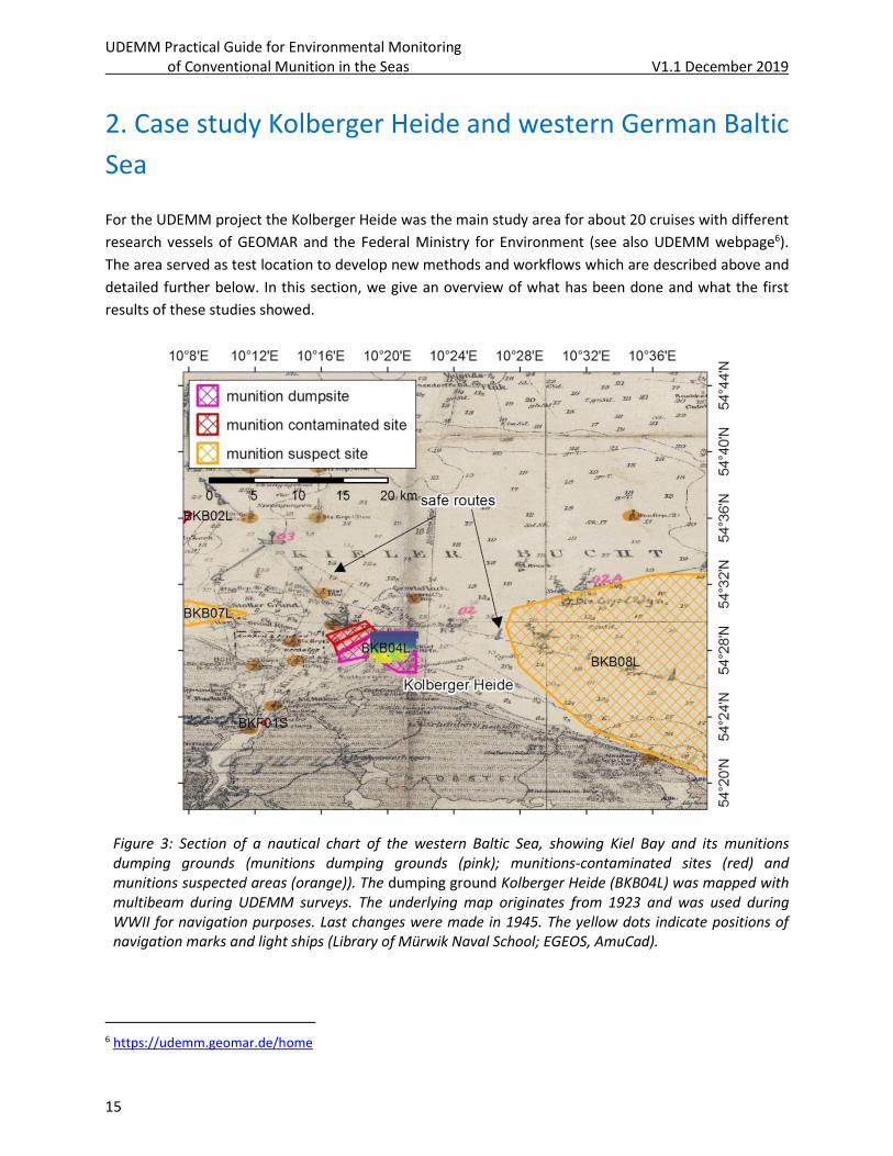
For the UDEMM project the Kolberger Heide was the main study area for about 20 cruises with different
research vessels of GEOMAR and the Federal Ministry for Environment (see also UDEMM webpage6).
The area served as test location to develop new methods and workflows which are described above and
detailed further below. In this section, we give an overview of what has been done and what the first
results of these studies showed.
Figure 3: Section of a nautical chart of the western Baltic Sea, showing Kiel Bay and its munitions dumping grounds (munitions dumping grounds (pink); munitions-contaminated sites (red) and munitions suspected areas (orange)). The dumping ground Kolberger Heide (BKB04L) was mapped with multibeam during UDEMM surveys. The underlying map originates from 1923 and was used during WWII for navigation purposes. Last changes were made in 1945. The yellow dots indicate positions of navigation marks and light ships (Library of Mürwik Naval School; EGEOS, AmuCad).
6 https://udemm.geomar.de/home
UDEMM Practical Guide for Environmental Monitoring of Conventional Munition in the Seas V1.1 December 2019
16
In October 2018, the UDEMM consortium went on an additional cruise along the German Baltic coast
with RV POSEIDON (cruise POS530 – MineMoni) and acquired a substantial set of water samples,
dropped bio-monitoring moorings and used a high-resolution ship-based multibeam system and AUV-
based camera observations to map selected areas in very high detail (Fehmarnsund and Bay of Lübeck;
Figure 3).
The sequence of the next subsections is organized in such a way as we believe a monitoring of a new,
largely unknown area should be done. During UDEMM itself, we did not follow the best methodology
structure, as the respective approaches still needed to be developed. At a late stage of the project, we
further got in contact with Uwe Wichert (Consultant BLANO, MELUND and HELCOM SUBMERGED) who
is an expert in WWI and WWII maritime war activities doing research in various archives in Germany and
the UK. Through his expertise we realized that an in depth historical survey of the type of ammunition
and their amounts that are/might be present in an area is of great importance for a better
interpretation of results. It also allows for a better informed comparison between different areas and
their joint impact on the environment.
2.1 History of the study area Kolberger Heide Responsible institute: BLANO & GEOMAR
Kampmeier et al. (in review) just recently presented an overview of the Kolberger Heide including its
historical analyses. Documents of the provincial and federal archives in Schleswig and Freiburg
(Germany) and the National Archive in Kew (UK) provide detailed information on the usage of the
Kolberger Heide area in the past. With regards to war activities, the Kolberger Heide was firstly
mentioned in the sea battle on 1 July 1644 during the Swedish-Danish war (1643-1645 CE). Before and
during WWI, it was only used for commercial fishing, as it was too shallow for the German fleet to enter
(Sections of nautical sea charts of the German Kriegsmarine, last changes in May 1945, Fachbibliothek
Marineschule Mürwik). It is possible that 28 cm training grenades (steel housing without explosives)
were introduced to the area during training exercises of the gun battery in Laboe. Apart from that, there
are no records of additional munitions entering the area until WWII.
The first records from this period report the introduction of munitions in 1940, when the British Royal
Air Force started bombing Kiel. Failed bombings, emergency overboard disposal and targeted attacks on
vessels and watch units occurred along the Marine Traffic Route 1. This traffic route extended from Kiel
to the eastern parts of the Baltic Sea (Figure 3) and was constantly surveyed and cleared by the German
Kriegsmarine by mine clearing vessels and airborne mine clearing systems. It was the only ‘safe’ path
vessels could use during times of war and was therefore an important target for the British Air Force.
However, the route was protected by German forces with onshore and vessel-based 12.8 cm anti-
aircraft guns. A number of these shells ended up as unexploded ordnance (UXO) in Kiel Bay and also in
the Kolberger Heide area. To obstruct vessel traffic, the British mined the Traffic Route 1, with as many
as 3,896 British mines, also targeting the Kolberger Heide (British Mining Operations 1939 - 1945).
Because of the high number of mines and resulting losses, commercial fishing was prohibited in
Kolberger Heide in 1942 (Bundesarchiv Militärarchiv Kriegstagebuch Sperrkommandant westliche
Ostsee). Bombing and mining activities continued until the end of the war in May 1945. After the war,
UDEMM Practical Guide for Environmental Monitoring of Conventional Munition in the Seas V1.1 December 2019
17
enormous quantities of captured arms and munitions were dumped into the sea, this was seen as the
fastest and at that time safest method to secure and dispose of the weapons. The dumping grounds in
German waters (North Sea and Baltic Sea) were chosen and approved on 29th July 1945, with Kolberger
Heide mentioned as the first dumping ground (documents from the national archive of the UK in Kew).
Following this decision, continuous sea-dumping of munitions occurred at Kolberger Heide. This
included torpedo heads and mines from the torpedo arsenals in Schleswig-Holstein. Documents from
the federal state of Schleswig-Holstein describe the dumping of about 24,000 metric tons of all kinds of
munitions in Kolberger Heide. Adding torpedo heads and mines, about 30,000 t of munitions have to be
assumed to be present at the site (Landesarchiv SL Akten des Kampfmittelräumdienstes). This includes
an array of ammunition types ranging from gun and pistol cartridges, artillery projectiles consisting of
grenades and propulsion cartridges, as well as anti-aircraft ammunition of 2 cm up to 40.6 cm calibre. In
addition, the Kolberger Heide site most likely contains explosive charges such as anti-tank and anti-
personnel mines, rifle grenades or bursting and hollow charges. Furthermore, bombs ranging from 1 kg
up to 500 and 1.000 kg in weight, rockets with diameters of up to 32 cm, as well as marine munitions
such as moored and ground mines, torpedo heads, whole torpedoes, and depth charges are present.
Some torpedoes that were formerly dumped in the area of Jägersberger Bridge were relocated to
Kolberger Heide and re-dumped. Also, a barge loaded with 500 tons of chemical munitions (grenades of
10.5 and 15 cm calibre) were sunk in the Little Belt. According to records, it was recovered and re-sunk
in the area of Kolberger Heide. In 1959, boxes with propellant charge powder stored on the upper deck
of the barge were salvaged, until the chemical munitions were discovered. After that the chemical
grenades were partially removed and the remainder relocated together with the barge to Geltinger Birk,
where everything was encased in concrete and finally sunk in the North Atlantic (Landesarchiv SL Akten
des Kampmittelräumdienstes).
As often when dealing with WWI and WWII dumped munition, the exact number and type of
ammunition (and manufacturer) is unknown and therefore all common explosives and propellant charge
powders used in WWII have to be assumed to be present at the Kolberger Heide site. This includes all
sorts of filling powder, amatol, ammonite, ammonal, grenade filling 88 and marine explosives such as
gun cotton (e.g. Schießwolle 36 and 39), special and testing explosives.
Since the munitions were manufactured from different kinds of material, it is not possible to predict the
precise state of the munitions housings. Thin-walled moored mines and cartridges may already be
heavily corroded, exposing explosive material to sea water; thick-walled artillery shells, bombs and
ground mines may yet still be intact.
After WWII, the Allies intended to only dump defused munition; however it cannot be taken for granted
that this was true for all dumped objects. Accidents including personal injuries and death occurred
during the dumping work, and thus it needs to be assumed that at least some of the handled munitions
were still armed. This is especially true for long-period delay detonators, mines with lead fuses or
pendulum impact ignition.
Additional regions similar to Kolberger Heide were chosen as munitions dumping grounds by the Allies;
these include areas offshore Schönhagen and Falshöft in the Bay of Lübeck/Bay of Neustadt. It is also
known that light-weight munitions like grenades were thrown overboard in Friedrichsort, Stollergrund,
Strande Bay, and en route to these dumping grounds. These actions are indicated by findings of
UDEMM Practical Guide for Environmental Monitoring of Conventional Munition in the Seas V1.1 December 2019
18
fishermen and the EOD service (BLMP Bericht 2011 and Akten des Landesarchivs SL) and demonstrate
the wide spread disposal of munitions in the south-western Baltic Sea that is now Germany territory.
Following WWII, Kolberger Heide was not used as a military training area anymore and is therefore not
affected by contamination with further munitions. However, munitions that were subsequently found
along marine traffic routes in Kiel Bay was defused and relocated to Kolberger Heide by the EOD service;
this practice is still ongoing and its results have been noticed during the UDEMM project by comparing
multibeam maps acquired at different times.
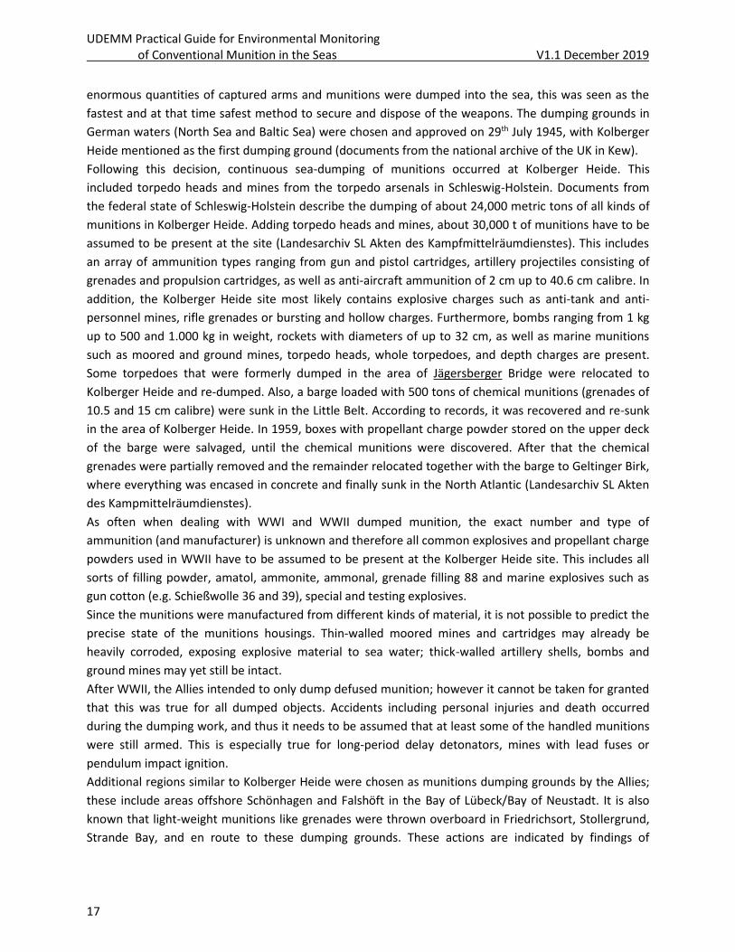
Table 3 Amunition type and explosive weights for dumped munitions in Kolberger Heide.
Mine type amount shell weight
kg explosive weight kg
ratio explosive/shell
total explosives tones
Sea mine large 316 220-280 300-350 0.51 - 0.61 102.70
Sea mine small 29 130 30 0.19 0.87
Ground mine A 1834 200-230 560-800 0.7 - 0.8 1,247.12
Ground mine B 181 900 200 0.18 36.20
Depth charges large 3000 80 60 ca. 58:42 % 180.00
Depth charges small
788 55 130 ca. 30:70 % 102.44
Bomb mine 1000 6 400 600 40:60 % 3.60
Bomb mine 250 31 125 125 50:50 % 3.88
British mine 110 200-400 90-500 0.18 - 0.71 32.45
Total 1709.255
2.2 Hydro-acoustic and visual mapping results Responsible institute: GEOMAR
As part of the scientific work in UDEMM, we tested two different kinds of state-of-the-art multibeam
systems, a NORBIT iWBMS and a RESON T50. Both systems performed well with respect to their
capacity, but most of the mapping finally occurred with the T50, which has a higher resolution (0.5°
along- and 1° across track). For high quality survey results, it was essential to properly reference all
sensors to each other and use undisturbed RTK correction for the navigation. The presented results
below have recently been submitted by Kampmeier et al. (in review).
For the compilation of the entire Kolberger Heide area 20 d of surveying were needed (Figure 3), that
were performed between 2016 and 2018. Repeating surveys in Nov. 2015, Feb. 2018 and June 2018
aimed at identifying potential migration of objects. The restricted dumping ground is located in the
south of the area in 5 - 14 m water depth on a shallow platform, which towards the north develops into
a more horizontal plain in 19 - 20 m water depth. Patches of algae, covering the seafloor with varying
density could be observed in underwater video profiles and show seasonal variability in their spatial
distribution. Small scale ripples of 5 cm height and 20 cm width indicate sediment transport on the
seafloor. Their crests are generally N-S oriented and thus perpendicular to the bottom current direction
(Figure 4).
UDEMM Practical Guide for Environmental Monitoring of Conventional Munition in the Seas V1.1 December 2019
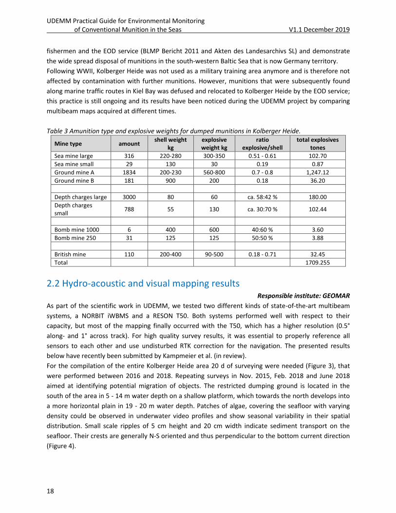
19
Figure 4 Left: a ripple field in Kolberger Heide. Right: Measuring the ripple height via a checker board. The black and white squares are of 2 cm size each. The observed ripples are ca 5 cm high and up to 20 cm wide. Their symmetric shape rather point to wave induced ripples, rather than formed by currents.
In 19 m water depth in the outer area of the dumping ground, otter trawling marks are clearly visible
inside the soft sediments and indicate significant fishing activities. This fishing method uses two boards
that are dragged across the seafloor to keep the trawling net open. Since 2004, the trawling is
prohibited in the Baltic Sea for areas more shallow than 20 m water depth or within 3 miles to the
coastline. Despite the ban, 10 - 100 h of otter board trawling were noted within this area in 2006 (Sell et
al., 2011). Even though Kolberger Heide is not one of the main fishing grounds in Kiel Bay, bottom
trawling seems to occur close to the official dumping ground and thus can potentially lead to object
displacement.
On local scale the bathymetry is characterized by a shallow platform, which extends from the shore and
declines with a slope of less than 1° towards the north. It builds a plain in 19 m water depth. Patches
that show increased rugosity (height differences of 2 - 4 cm) and ripple-like structures are present in the
feature-scale morphology. Those areas produce high backscatter intensities and contain increased
amounts of rocks. As the underwater environment of Kolberger Heide is strongly affected by
anthropogenic use, artificial objects and remnants of activities are present on local and feature-scale.
There are explosion craters with average diameters of 20 m and depths of 1.5 m, which can be observed
as clusters or isolated craters across the entire study area. Craters were formed by in-situ destructions
that partially acted as tests for bubble curtain experiments. Bubble curtains significantly decrease the
sound energy of detonations and thus particularly protect marine mammals (Würsig et al., 2000).
Remnants of these bubble curtains in form of hoses and anchor stones were left on the seafloor; they
can be reactivated if needed. Other types of feature-scale objects are all kind of UXO and dumped
munitions in high numbers. Depending on the ammunition type, accurate identification is challenging to
a varying degree. Three hot spot areas have been detected. The first area is composed of ~70 defused
moored mines, piled up to a mound-like structure of 30 m length and 15 m width. Its height above the
surrounding seafloor is about 1.5 m. The second highly contaminated area is located at a cluster of
detonation craters (Figure 5). At this location around 90 munition objects of different types ranging from
German and English ground mines over torpedo heads, water bombs to moored mines can be found.
UDEMM Practical Guide for Environmental Monitoring of Conventional Munition in the Seas V1.1 December 2019
20
Some of these objects have been brought to the dumping ground after being defused by the EOD
service. The third area of around 150 m2 in size shows ca. 100 objects of 1 m by 0.6 m.
Initial validation dives identified these objects as aerial bombs, possibly fused. A high number of
additional suspicious objects can be found all over the research area. Moored mines occur as spherical
shaped objects with ca 1.2 m diameter all over the existing bathymetric data set. Due to their size and
elongated shape, ground mines and torpedoes can be identified rather easily. Smaller objects such as
bombs and torpedo heads are not as easily identified and require validation by divers or underwater
video. Joint observation of derivatives with bathymetric data, can greatly enhance the speed of
detecting and identifying munition objects. Slope, surface area and curvature highlight distinct objects
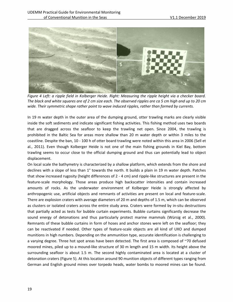
as rocks and munitions on the seafloor very clearly (Figure 5).
Figure 5 A) The high resolution bathymetry reveals morphological features like five explosion craters of around 25 m diameter. Furthermore, differences in the seafloor texture like patches of increased rugosity are visible. B) Close-up of ground mines in and around explosion craters (feature scale).
2.3 Munitions compounds in water, sediment and biota Responsible institute: GEOMAR
Dissolved MC in the water column: Dissolved MCs were detectible in nearly all water column samples
collected during the UDEMM project. Concentrations showed a range nearly exceeding nine orders-of-
magnitude (Figure 6), most likely due to rapid mixing and dilution. Most of the samples showed TNT
concentrations on the order of 1-10 pM, highlighting the critical need to use ultra-sensitive detection
methods such as those developed during UDEMM. Previous results showed that MC distributions in the
water column were highly variable in both space and time and that high resolution sampling is required
to adequately monitor the regional magnitude and extent of contaminant plumes from underwater
munitions dumping grounds. As a result, the sample collection and processing method that had been
developed earlier during UDEMM (and published in Gledhill et al., 2019) were modified to reduce
processing time and facilitate higher frequency sampling (see Section 4.7).
UDEMM Practical Guide for Environmental Monitoring of Conventional Munition in the Seas V1.1 December 2019
21
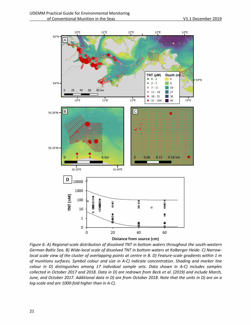
Figure 6: A) Regional-scale distribution of dissolved TNT in bottom waters throughout the south-western German Baltic Sea. B) Wide-local scale of dissolved TNT in bottom waters at Kolberger Heide. C) Narrow-local scale view of the cluster of overlapping points at centre in B. D) Feature-scale gradients within 1 m of munitions surfaces. Symbol colour and size in A-C) indicate concentration. Shading and marker line colour in D) distinguishes among 17 individual sample sets. Data shown in A-C) includes samples collected in October 2017 and 2018. Data in D) are redrawn from Beck et al. (2019) and include March, June, and October 2017. Additional data in D) are from October 2018. Note that the units in D) are on a log-scale and are 1000-fold higher than in A-C).
UDEMM Practical Guide for Environmental Monitoring of Conventional Munition in the Seas V1.1 December 2019
22
At the regional scale (Figure 6A), clear gradients were evident in TNT concentration. Areas with
munitions dumping ground (e.g., Kolberger Heide; Bay of Lübeck) or known munitions contamination
tended to show the highest concentrations (up to 354 pM for TNT). Nonetheless, there were marked
differences among dumping ground, illustrated by the nearly order-of-magnitude difference between
maximum concentrations observed in October 2018 in Kolberger Heide (354 pM) compared with the
Bay of Lübeck (43 pM). This is the case, despite estimates that the Bay of Lübeck contains about double
the amount present in Kolberger Heide (Böttcher et al., 2011). TNT concentrations were lowest in the
Arkona Basin and the Mecklenburg Bight, likely as a result of their deeper water column and greater
distance from munitions sites. Water exchange through the central channel and Belt Sea (north and
northeast of Fehmarn) dilutes contamination originating close to coastlines, although samples collected
north and northeast of Fehmarn showed substantial TNT enrichment.
The widespread presence of munitions on the Baltic seafloor make it challenging to link specific MC
sources to plumes of dissolved MCs in the water column. Elevated concentrations oberved in the far
western basin, and the wide dispersion of MCs on wide local scales (Figure 6B) imply long-range
transport of MCs. This must occur on relatively short time scales, before loss by microbial or abiotic
degradation or sorption and sedimentation with particles occur.
Loss of MCs through mechanisms such as degradation or sorption is likely to depend on site-specific
characteristics such as temperature and salinity. Evaluating the impact of MC release on ecological
systems requires constraint of potential long-range transport and chemical residence times. A number
of simple experiements were conducted during UDEMM (see below) to provide an approximation of
these controls and a quantitative constraint for modelling purposes.
On the local scale (0.05 - 5 km) in Kolberger Heide, water column TNT distributions show some
indication of gradients around known munitions hotspots (Figure 6 and Figure 7). A general east-west
increase in concentration cross the entire Kolberger Heide site may reflect enrichment of water traveling
along the predominant current direction (Figure 7B. However, on the small local scale (10s to 100s of
meters), gradients seem to be smoothed out by water mixing. For example, nine samples collected
within 200 m around a pile of some 70 - 90 sea mines show no clear gradient in dissolved TNT (Figure 7c,
Figure 8). This suggests that on such spatial scales, mixing is rapid relative to both input from the
munitions source as well as removal mechanisms such as degradation.
A variety of explosive compounds in an even more extensive array of explosive mixtures exist, with more
than 500 formulations manufactures (Haas and Thieme, 1996). Most organic explosives also undergo
degradation or transformation to daughter compounds. Many of these daughter compounds are equally
or more toxic than the parent, or toxicity is unknown. Such alteration can occur on a time scale of hours
to days. It may thus be possible to have high influx, but low water column inventories of the parent MC.
Monitoring only the parent MCs would underestimate the total chemical release. This emphasises the
importance of multi-compound chemical analyses for evaluating chemical emission from underwater
munitions.
The method developed during UDEMM (Gledhill et al., 2019) targets 17 compounds, including both a
variety of explosives as well as several daughter product compounds. This was important, to elucidate
chemical release trends across all spatial scales.
UDEMM Practical Guide for Environmental Monitoring of Conventional Munition in the Seas V1.1 December 2019
23
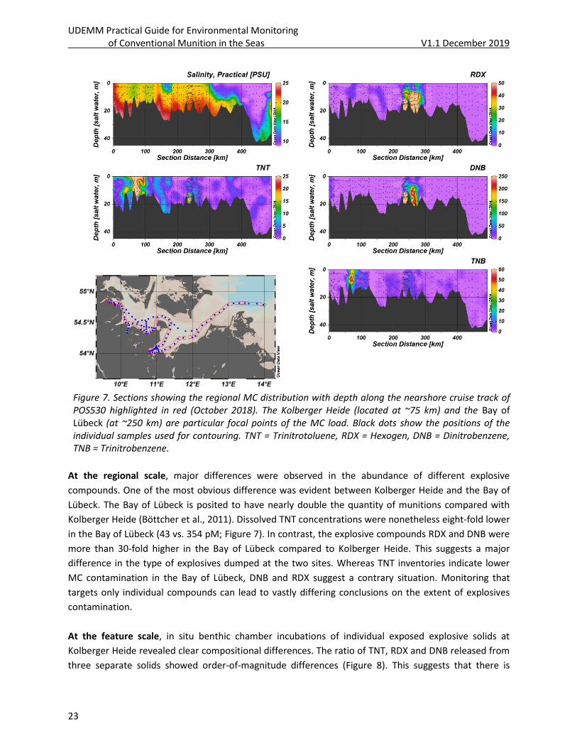
Figure 7. Sections showing the regional MC distribution with depth along the nearshore cruise track of POS530 highlighted in red (October 2018). The Kolberger Heide (located at ~75 km) and the Bay of Lübeck (at ~250 km) are particular focal points of the MC load. Black dots show the positions of the individual samples used for contouring. TNT = Trinitrotoluene, RDX = Hexogen, DNB = Dinitrobenzene, TNB = Trinitrobenzene.
At the regional scale, major differences were observed in the abundance of different explosive
compounds. One of the most obvious difference was evident between Kolberger Heide and the Bay of
Lübeck. The Bay of Lübeck is posited to have nearly double the quantity of munitions compared with
Kolberger Heide (Böttcher et al., 2011). Dissolved TNT concentrations were nonetheless eight-fold lower
in the Bay of Lübeck (43 vs. 354 pM; Figure 7). In contrast, the explosive compounds RDX and DNB were
more than 30-fold higher in the Bay of Lübeck compared to Kolberger Heide. This suggests a major
difference in the type of explosives dumped at the two sites. Whereas TNT inventories indicate lower
MC contamination in the Bay of Lübeck, DNB and RDX suggest a contrary situation. Monitoring that
targets only individual compounds can lead to vastly differing conclusions on the extent of explosives
contamination.
At the feature scale, in situ benthic chamber incubations of individual exposed explosive solids at
Kolberger Heide revealed clear compositional differences. The ratio of TNT, RDX and DNB released from
three separate solids showed order-of-magnitude differences (Figure 8). This suggests that there is

UDEMM Practical Guide for Environmental Monitoring of Conventional Munition in the Seas V1.1 December 2019
24
heterogeneity in explosives dumped at individual sites as well as among different sites. Strategies to
monitor the overall chemical release from underwater munitions must therefore take into account
spatial variability in the explosive source types.
Figure 8: Mass ratio of RDX and DNB to TNT observed in three in situ benthic chamber incubations of different explosive solids.
Figure 9: A) Regional-scale distribution of TNT, ADNT and DANT in surface sediments throughout the Kiel and Eckernförde Bights. B) Wide-local scale of TNT, ADNT and DANT in surface sediments at Kolberger Heide. C) Narrow-local scale view of the main Kolberger Heide site. The cluster of points near the centre is a transect across the mine mound as described above. Symbol shading and size indicate MC content and colour distinguishes among the three compounds.
UDEMM Practical Guide for Environmental Monitoring of Conventional Munition in the Seas V1.1 December 2019
25
Local retention of sediment MCs is consistent with the pattern observed at the km-scale (Figure 9b).
Elevated concentrations were observed within kilometres of munitions hotspots identified by seafloor
mapping, but declined rapidly away from the central source (Figure 9b). In contrast, enormous
heterogeneity was observed at the sub-km scale (Figure 9c). Samples separated by 10s of meters
showed as much variability as transects separated by several hundred meters.
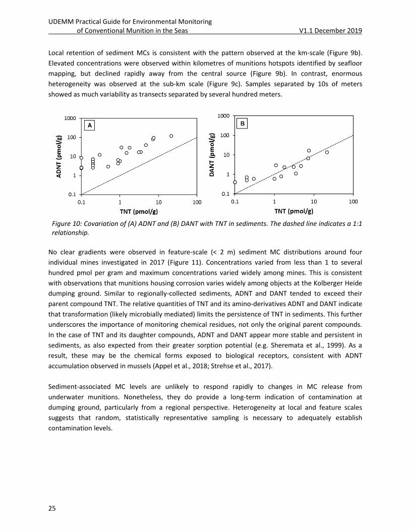
Figure 10: Covariation of (A) ADNT and (B) DANT with TNT in sediments. The dashed line indicates a 1:1 relationship.
No clear gradients were observed in feature-scale (< 2 m) sediment MC distributions around four
individual mines investigated in 2017 (Figure 11). Concentrations varied from less than 1 to several
hundred pmol per gram and maximum concentrations varied widely among mines. This is consistent
with observations that munitions housing corrosion varies widely among objects at the Kolberger Heide
dumping ground. Similar to regionally-collected sediments, ADNT and DANT tended to exceed their
parent compound TNT. The relative quantities of TNT and its amino-derivatives ADNT and DANT indicate
that transformation (likely microbially mediated) limits the persistence of TNT in sediments. This further
underscores the importance of monitoring chemical residues, not only the original parent compounds.
In the case of TNT and its daughter compounds, ADNT and DANT appear more stable and persistent in
sediments, as also expected from their greater sorption potential (e.g. Sheremata et al., 1999). As a
result, these may be the chemical forms exposed to biological receptors, consistent with ADNT
accumulation observed in mussels (Appel et al., 2018; Strehse et al., 2017).
Sediment-associated MC levels are unlikely to respond rapidly to changes in MC release from
underwater munitions. Nonetheless, they do provide a long-term indication of contamination at
dumping ground, particularly from a regional perspective. Heterogeneity at local and feature scales
suggests that random, statistically representative sampling is necessary to adequately establish
contamination levels.

UDEMM Practical Guide for Environmental Monitoring of Conventional Munition in the Seas V1.1 December 2019
26
Figure 11: Examples of MC content in surface sediments collected radially around individual munitions. Colours indicate TNT (red), ADNT (green; a transformation product of TNT) and DANT (blue; a transformation product of ADNT). Circle sizes indicate MC content; note different scales among figures. Molar units are used to allow direct comparison of the different compound amounts.
Source term – Dissolution: Dissolution of solid explosives is the principle control factor on MC emission
from underwater munitions. Dissolution rates are affected by physicochemical conditions such as
temperature, salinity and mixing energy, as well as explosive chemical formulation (Lynch et al., 2001;
Lever et al., 2005; Monteil-Rivera et al., 2010; Dontsova et al., 2006). All other conditions equal, MC
release may therefore be highly site-specific. In UDEMM, multiple approaches were used to quantify
dissolution fluxes. In situ dissolution was measured directly by MC release from exposed explosives
enclosed within a benthic chamber (e.g. Figure 12). Feature-scale gradients (Figure 6d) were also fit with
a simple steady-state model to estimate dissolution fluxes. These in situ methods revealed fluxes that
were substantially lower when compared to laboratory experiments reported in the literature (Beck et
al., 2019). The discrepancy most likely resulted from lower mixing energy in situ compared to laboratory
conditions.
Figure 12: Increase of dissolved TNT in a benthic chamber enclosing an exposed explosive solid. The dissolution flux calculated from the observed trend is also indicated.
UDEMM Practical Guide for Environmental Monitoring of Conventional Munition in the Seas V1.1 December 2019
27
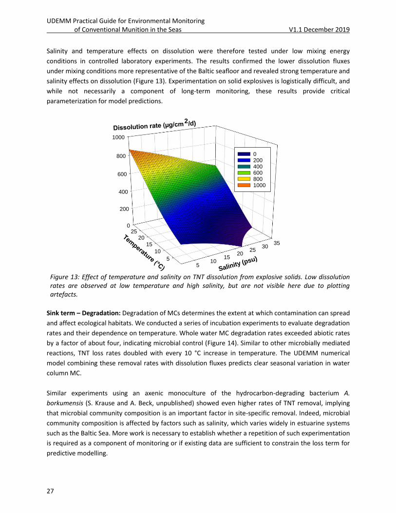
Salinity and temperature effects on dissolution were therefore tested under low mixing energy
conditions in controlled laboratory experiments. The results confirmed the lower dissolution fluxes
under mixing conditions more representative of the Baltic seafloor and revealed strong temperature and
salinity effects on dissolution (Figure 13). Experimentation on solid explosives is logistically difficult, and
while not necessarily a component of long-term monitoring, these results provide critical
parameterization for model predictions.
Figure 13: Effect of temperature and salinity on TNT dissolution from explosive solids. Low dissolution rates are observed at low temperature and high salinity, but are not visible here due to plotting artefacts.
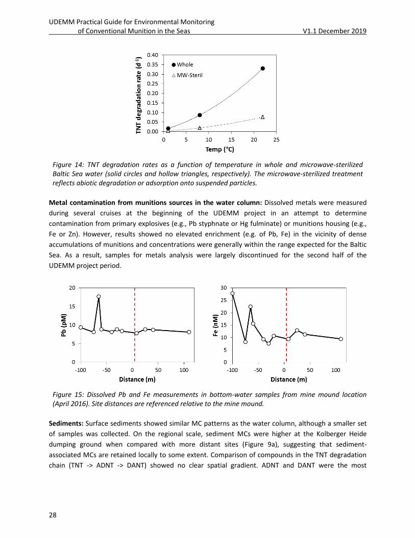
Sink term – Degradation: Degradation of MCs determines the extent at which contamination can spread
and affect ecological habitats. We conducted a series of incubation experiments to evaluate degradation
rates and their dependence on temperature. Whole water MC degradation rates exceeded abiotic rates
by a factor of about four, indicating microbial control (Figure 14). Similar to other microbially mediated
reactions, TNT loss rates doubled with every 10 °C increase in temperature. The UDEMM numerical
model combining these removal rates with dissolution fluxes predicts clear seasonal variation in water
column MC.
Similar experiments using an axenic monoculture of the hydrocarbon-degrading bacterium A.
borkumensis (S. Krause and A. Beck, unpublished) showed even higher rates of TNT removal, implying
that microbial community composition is an important factor in site-specific removal. Indeed, microbial
community composition is affected by factors such as salinity, which varies widely in estuarine systems
such as the Baltic Sea. More work is necessary to establish whether a repetition of such experimentation
is required as a component of monitoring or if existing data are sufficient to constrain the loss term for
predictive modelling.
0
200
400
600
800
1000
510
1520
2530
35
5
10
15
2025
Dissolution rate (µg/cm2/d)
Salinity (psu)
Temperature (°C)
0 200 400 600 800 1000
UDEMM Practical Guide for Environmental Monitoring of Conventional Munition in the Seas V1.1 December 2019
28
Figure 14: TNT degradation rates as a function of temperature in whole and microwave-sterilized Baltic Sea water (solid circles and hollow triangles, respectively). The microwave-sterilized treatment reflects abiotic degradation or adsorption onto suspended particles.
Metal contamination from munitions sources in the water column: Dissolved metals were measured
during several cruises at the beginning of the UDEMM project in an attempt to determine
contamination from primary explosives (e.g., Pb styphnate or Hg fulminate) or munitions housing (e.g.,
Fe or Zn). However, results showed no elevated enrichment (e.g. of Pb, Fe) in the vicinity of dense
accumulations of munitions and concentrations were generally within the range expected for the Baltic
Sea. As a result, samples for metals analysis were largely discontinued for the second half of the
UDEMM project period.
Figure 15: Dissolved Pb and Fe measurements in bottom-water samples from mine mound location (April 2016). Site distances are referenced relative to the mine mound.
Sediments: Surface sediments showed similar MC patterns as the water column, although a smaller set
of samples was collected. On the regional scale, sediment MCs were higher at the Kolberger Heide
dumping ground when compared with more distant sites (Figure 9a), suggesting that sediment-
associated MCs are retained locally to some extent. Comparison of compounds in the TNT degradation
chain (TNT -> ADNT -> DANT) showed no clear spatial gradient. ADNT and DANT were the most
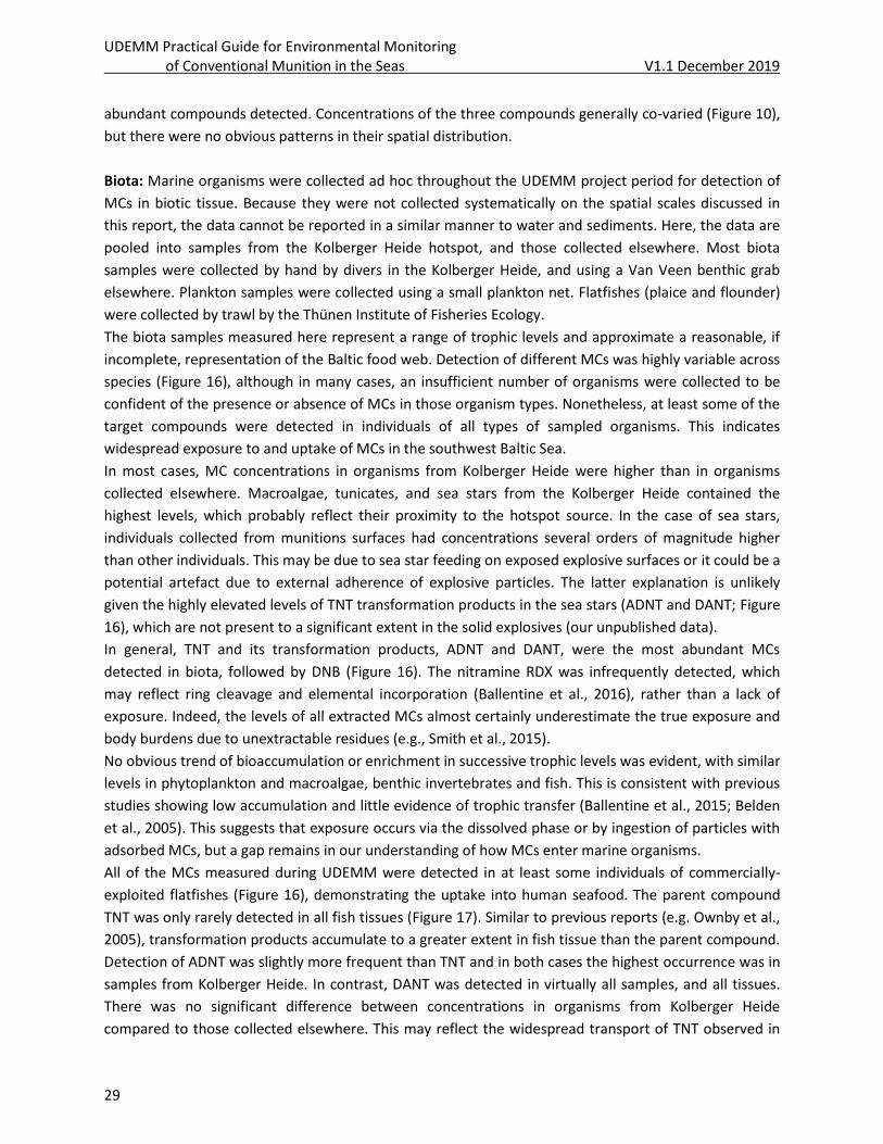
UDEMM Practical Guide for Environmental Monitoring of Conventional Munition in the Seas V1.1 December 2019
29
abundant compounds detected. Concentrations of the three compounds generally co-varied (Figure 10),
but there were no obvious patterns in their spatial distribution.
Biota: Marine organisms were collected ad hoc throughout the UDEMM project period for detection of
MCs in biotic tissue. Because they were not collected systematically on the spatial scales discussed in
this report, the data cannot be reported in a similar manner to water and sediments. Here, the data are
pooled into samples from the Kolberger Heide hotspot, and those collected elsewhere. Most biota
samples were collected by hand by divers in the Kolberger Heide, and using a Van Veen benthic grab
elsewhere. Plankton samples were collected using a small plankton net. Flatfishes (plaice and flounder)
were collected by trawl by the Thünen Institute of Fisheries Ecology.
The biota samples measured here represent a range of trophic levels and approximate a reasonable, if
incomplete, representation of the Baltic food web. Detection of different MCs was highly variable across
species (Figure 16), although in many cases, an insufficient number of organisms were collected to be
confident of the presence or absence of MCs in those organism types. Nonetheless, at least some of the
target compounds were detected in individuals of all types of sampled organisms. This indicates
widespread exposure to and uptake of MCs in the southwest Baltic Sea.
In most cases, MC concentrations in organisms from Kolberger Heide were higher than in organisms
collected elsewhere. Macroalgae, tunicates, and sea stars from the Kolberger Heide contained the
highest levels, which probably reflect their proximity to the hotspot source. In the case of sea stars,
individuals collected from munitions surfaces had concentrations several orders of magnitude higher
than other individuals. This may be due to sea star feeding on exposed explosive surfaces or it could be a
potential artefact due to external adherence of explosive particles. The latter explanation is unlikely
given the highly elevated levels of TNT transformation products in the sea stars (ADNT and DANT; Figure
16), which are not present to a significant extent in the solid explosives (our unpublished data).
In general, TNT and its transformation products, ADNT and DANT, were the most abundant MCs
detected in biota, followed by DNB (Figure 16). The nitramine RDX was infrequently detected, which
may reflect ring cleavage and elemental incorporation (Ballentine et al., 2016), rather than a lack of
exposure. Indeed, the levels of all extracted MCs almost certainly underestimate the true exposure and
body burdens due to unextractable residues (e.g., Smith et al., 2015).
No obvious trend of bioaccumulation or enrichment in successive trophic levels was evident, with similar
levels in phytoplankton and macroalgae, benthic invertebrates and fish. This is consistent with previous
studies showing low accumulation and little evidence of trophic transfer (Ballentine et al., 2015; Belden
et al., 2005). This suggests that exposure occurs via the dissolved phase or by ingestion of particles with
adsorbed MCs, but a gap remains in our understanding of how MCs enter marine organisms.
All of the MCs measured during UDEMM were detected in at least some individuals of commercially-
exploited flatfishes (Figure 16), demonstrating the uptake into human seafood. The parent compound
TNT was only rarely detected in all fish tissues (Figure 17). Similar to previous reports (e.g. Ownby et al.,
2005), transformation products accumulate to a greater extent in fish tissue than the parent compound.
Detection of ADNT was slightly more frequent than TNT and in both cases the highest occurrence was in
samples from Kolberger Heide. In contrast, DANT was detected in virtually all samples, and all tissues.
There was no significant difference between concentrations in organisms from Kolberger Heide
compared to those collected elsewhere. This may reflect the widespread transport of TNT observed in
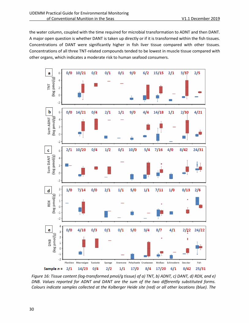
UDEMM Practical Guide for Environmental Monitoring of Conventional Munition in the Seas V1.1 December 2019
30
the water column, coupled with the time required for microbial transformation to ADNT and then DANT.
A major open question is whether DANT is taken up directly or if it is transformed within the fish tissues.
Concentrations of DANT were significantly higher in fish liver tissue compared with other tissues.
Concentrations of all three TNT-related compounds tended to be lowest in muscle tissue compared with
other organs, which indicates a moderate risk to human seafood consumers.
Figure 16: Tissue content (log-transformed pmol/g tissue) of a) TNT, b) ADNT, c) DANT, d) RDX, and e) DNB. Values reported for ADNT and DANT are the sum of the two differently substituted forms. Colours indicate samples collected at the Kolberger Heide site (red) or all other locations (blue). The

UDEMM Practical Guide for Environmental Monitoring of Conventional Munition in the Seas V1.1 December 2019
31
sample n shown below the organism type names on the abscissa indicates the total number of organisms that were collected (“non-KH/KH”). The numbers shown in each plot above the data boxes represent the number of samples of each type in which the corresponding MCs was actually detected (i.e. the number of data points included in each box-and-whisker set). Median MC content is indicated by the horizontal line within the boxes. Upper and lower bounds of the boxes indicate the upper and lower quartiles, and the whiskers indicate smallest and largest samples 1.5 times the interquartile range. Dots indicate data points outside this range.
Figure 17: Tissue content (log-transformed pmol/g tissue) of a) TNT, b) ADNT, and c) DANT, in different organs in plaice and flounder. Values for ADNT and DANT are the sum of the two differently substituted forms. Colours indicate samples collected at the Kolberger Heide site (red) or all other locations (blue). The sample n shown below the tissue type names on the abscissa indicates the total number of organisms that were collected (“non-KH/KH”). The numbers shown in each plot above the data boxes represent the number of samples of each type in which the corresponding MCs was actually detected (i.e., the number of data points included in each box-and-whisker set). Median MC content is indicated by the horizontal line with the boxes. Upper and lower bounds of the boxes indicate the upper and lower quartiles, and the whiskers indicate smallest and largest samples 1.5 times the interquartile range. Dots indicate data points outside this range.
References
Appel, D., Strehse, J. S., Martin, H. J., & Maser, E. (2018). Bioaccumulation of 2, 4, 6-trinitrotoluene (TNT) and its metabolites
leaking from corroded munition in transplanted blue mussels (M. edulis). Marine pollution bulletin, 135, 1072-1078.
Ballentine, M., Tobias, C., Vlahos, P., Smith, R., & Cooper, C. (2015). Bioconcentration of TNT and RDX in coastal marine biota.
Archives of environmental contamination and toxicology, 68(4), 718-728.
Ballentine, M. L., Ariyarathna, T., Smith, R. W., Cooper, C., Vlahos, P., Fallis, S., Groshens, T.J. & Tobias, C. (2016). Uptake and
fate of hexahydro-1, 3, 5-trinitro-1, 3, 5-triazine (RDX) in coastal marine biota determined using a stable isotopic tracer,
15N–[RDX]. Chemosphere, 153, 28-38.
Beck, A. J., van der Lee, E. M., Eggert, A., Stamer, B., Gledhill, M., Schlosser, C., & Achterberg, E. P. 2019. In situ measurements
of explosive compound dissolution fluxes from exposed munition material in the Baltic Sea. Environmental science &
technology. 53, 5652−5660.
Belden, J. B., Ownby, D. R., Lotufo, G. R., & Lydy, M. J. (2005). Accumulation of trinitrotoluene (TNT) in aquatic organisms: Part
2—Bioconcentration in aquatic invertebrates and potential for trophic transfer to channel catfish (Ictalurus punctatus).
Chemosphere, 58(9), 1161-1168.
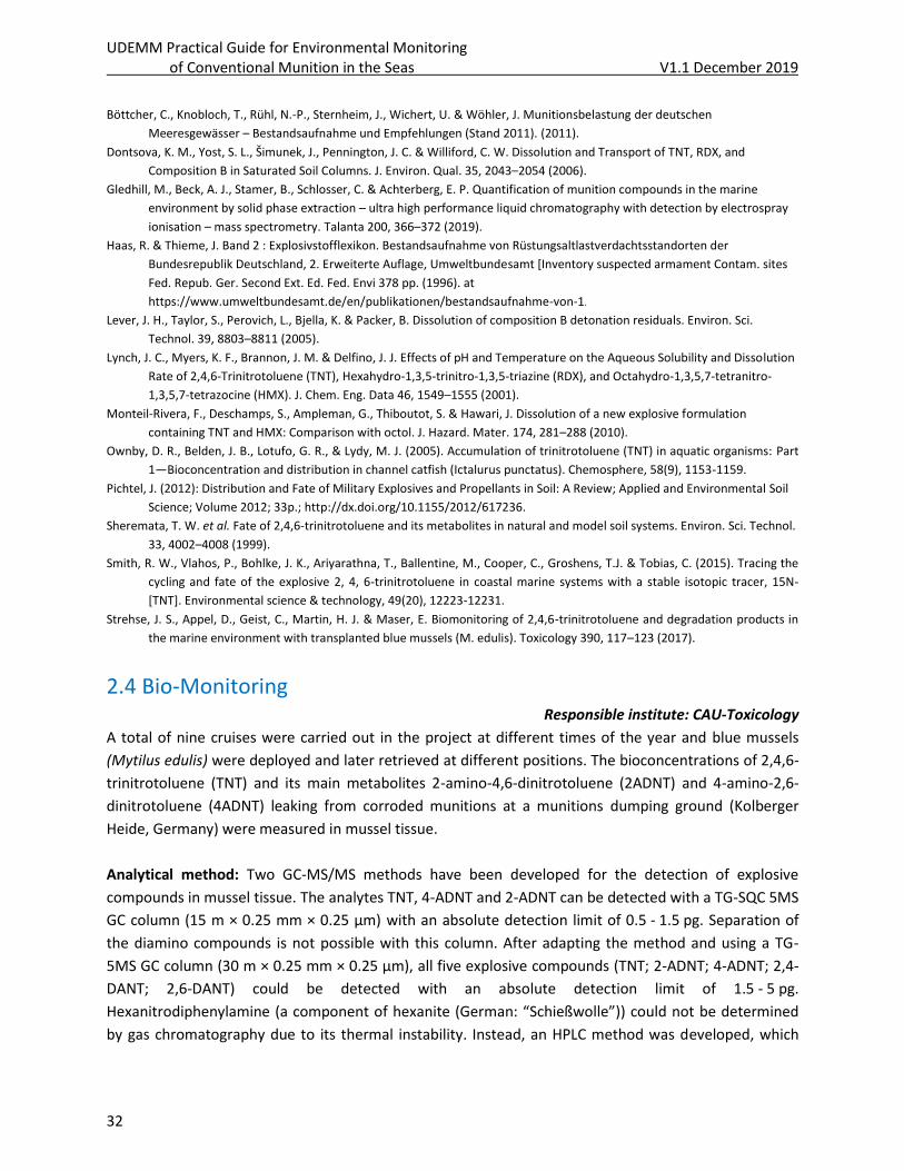
UDEMM Practical Guide for Environmental Monitoring of Conventional Munition in the Seas V1.1 December 2019
32
Böttcher, C., Knobloch, T., Rühl, N.-P., Sternheim, J., Wichert, U. & Wöhler, J. Munitionsbelastung der deutschen
Meeresgewässer – Bestandsaufnahme und Empfehlungen (Stand 2011). (2011).
Dontsova, K. M., Yost, S. L., Šimunek, J., Pennington, J. C. & Williford, C. W. Dissolution and Transport of TNT, RDX, and
Composition B in Saturated Soil Columns. J. Environ. Qual. 35, 2043–2054 (2006).
Gledhill, M., Beck, A. J., Stamer, B., Schlosser, C. & Achterberg, E. P. Quantification of munition compounds in the marine
environment by solid phase extraction – ultra high performance liquid chromatography with detection by electrospray
ionisation – mass spectrometry. Talanta 200, 366–372 (2019).
Haas, R. & Thieme, J. Band 2 : Explosivstofflexikon. Bestandsaufnahme von Rüstungsaltlastverdachtsstandorten der
Bundesrepublik Deutschland, 2. Erweiterte Auflage, Umweltbundesamt [Inventory suspected armament Contam. sites
Fed. Repub. Ger. Second Ext. Ed. Fed. Envi 378 pp. (1996). at
https://www.umweltbundesamt.de/en/publikationen/bestandsaufnahme-von-1.
Lever, J. H., Taylor, S., Perovich, L., Bjella, K. & Packer, B. Dissolution of composition B detonation residuals. Environ. Sci.
Technol. 39, 8803–8811 (2005).
Lynch, J. C., Myers, K. F., Brannon, J. M. & Delfino, J. J. Effects of pH and Temperature on the Aqueous Solubility and Dissolution
Rate of 2,4,6-Trinitrotoluene (TNT), Hexahydro-1,3,5-trinitro-1,3,5-triazine (RDX), and Octahydro-1,3,5,7-tetranitro-
1,3,5,7-tetrazocine (HMX). J. Chem. Eng. Data 46, 1549–1555 (2001).
Monteil-Rivera, F., Deschamps, S., Ampleman, G., Thiboutot, S. & Hawari, J. Dissolution of a new explosive formulation
containing TNT and HMX: Comparison with octol. J. Hazard. Mater. 174, 281–288 (2010).
Ownby, D. R., Belden, J. B., Lotufo, G. R., & Lydy, M. J. (2005). Accumulation of trinitrotoluene (TNT) in aquatic organisms: Part
1—Bioconcentration and distribution in channel catfish (Ictalurus punctatus). Chemosphere, 58(9), 1153-1159.
Pichtel, J. (2012): Distribution and Fate of Military Explosives and Propellants in Soil: A Review; Applied and Environmental Soil
Science; Volume 2012; 33p.; http://dx.doi.org/10.1155/2012/617236.
Sheremata, T. W. et al. Fate of 2,4,6-trinitrotoluene and its metabolites in natural and model soil systems. Environ. Sci. Technol.
33, 4002–4008 (1999).
Smith, R. W., Vlahos, P., Bohlke, J. K., Ariyarathna, T., Ballentine, M., Cooper, C., Groshens, T.J. & Tobias, C. (2015). Tracing the
cycling and fate of the explosive 2, 4, 6-trinitrotoluene in coastal marine systems with a stable isotopic tracer, 15N-
[TNT]. Environmental science & technology, 49(20), 12223-12231. Strehse, J. S., Appel, D., Geist, C., Martin, H. J. & Maser, E. Biomonitoring of 2,4,6-trinitrotoluene and degradation products in
the marine environment with transplanted blue mussels (M. edulis). Toxicology 390, 117–123 (2017).
2.4 Bio-Monitoring Responsible institute: CAU-Toxicology
A total of nine cruises were carried out in the project at different times of the year and blue mussels
(Mytilus edulis) were deployed and later retrieved at different positions. The bioconcentrations of 2,4,6-
trinitrotoluene (TNT) and its main metabolites 2-amino-4,6-dinitrotoluene (2ADNT) and 4-amino-2,6-
dinitrotoluene (4ADNT) leaking from corroded munitions at a munitions dumping ground (Kolberger
Heide, Germany) were measured in mussel tissue.
Analytical method: Two GC-MS/MS methods have been developed for the detection of explosive
compounds in mussel tissue. The analytes TNT, 4-ADNT and 2-ADNT can be detected with a TG-SQC 5MS
GC column (15 m × 0.25 mm × 0.25 μm) with an absolute detection limit of 0.5 - 1.5 pg. Separation of
the diamino compounds is not possible with this column. After adapting the method and using a TG-
5MS GC column (30 m × 0.25 mm × 0.25 µm), all five explosive compounds (TNT; 2-ADNT; 4-ADNT; 2,4-
DANT; 2,6-DANT) could be detected with an absolute detection limit of 1.5 - 5 pg.
Hexanitrodiphenylamine (a component of hexanite (German: “Schießwolle”)) could not be determined
by gas chromatography due to its thermal instability. Instead, an HPLC method was developed, which
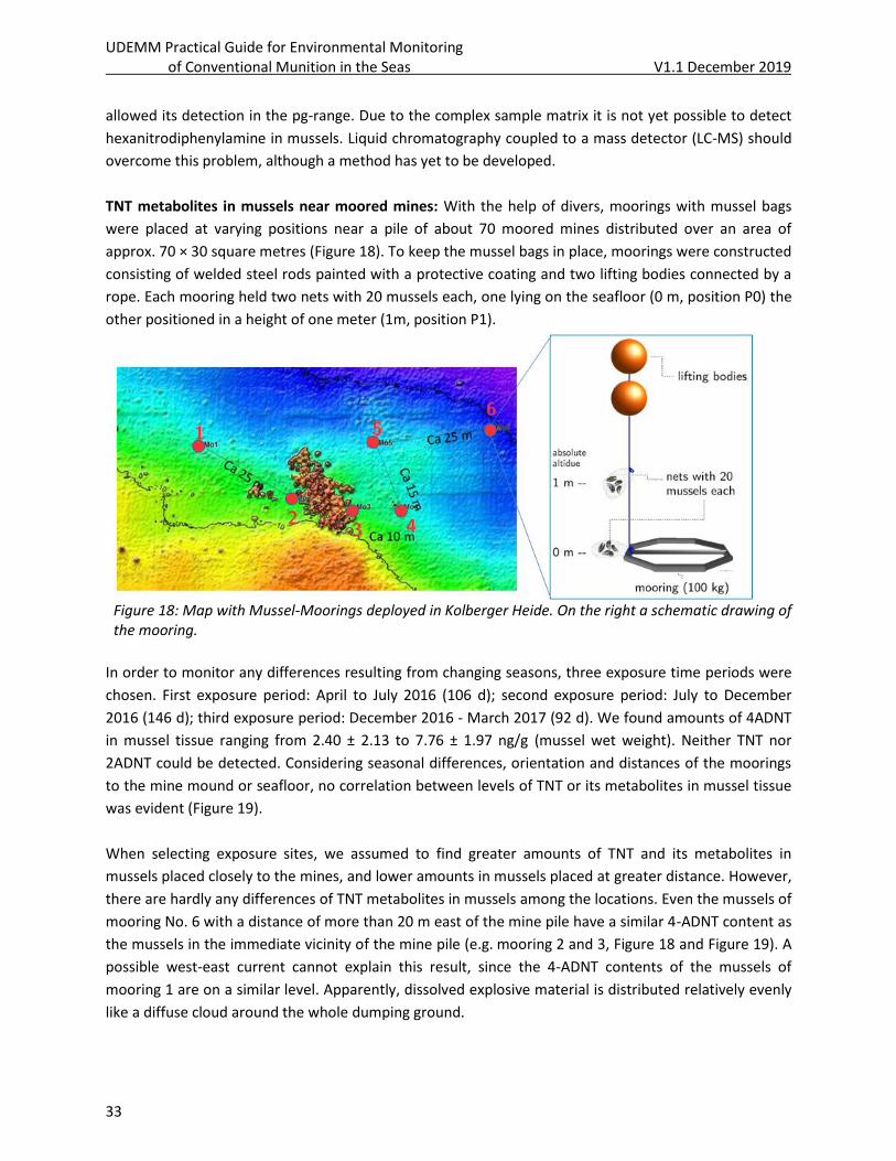
UDEMM Practical Guide for Environmental Monitoring of Conventional Munition in the Seas V1.1 December 2019
33
allowed its detection in the pg-range. Due to the complex sample matrix it is not yet possible to detect
hexanitrodiphenylamine in mussels. Liquid chromatography coupled to a mass detector (LC-MS) should
overcome this problem, although a method has yet to be developed.
TNT metabolites in mussels near moored mines: With the help of divers, moorings with mussel bags
were placed at varying positions near a pile of about 70 moored mines distributed over an area of
approx. 70 × 30 square metres (Figure 18). To keep the mussel bags in place, moorings were constructed
consisting of welded steel rods painted with a protective coating and two lifting bodies connected by a
rope. Each mooring held two nets with 20 mussels each, one lying on the seafloor (0 m, position P0) the
other positioned in a height of one meter (1m, position P1).
Figure 18: Map with Mussel-Moorings deployed in Kolberger Heide. On the right a schematic drawing of the mooring.
In order to monitor any differences resulting from changing seasons, three exposure time periods were
chosen. First exposure period: April to July 2016 (106 d); second exposure period: July to December
2016 (146 d); third exposure period: December 2016 - March 2017 (92 d). We found amounts of 4ADNT
in mussel tissue ranging from 2.40 ± 2.13 to 7.76 ± 1.97 ng/g (mussel wet weight). Neither TNT nor
2ADNT could be detected. Considering seasonal differences, orientation and distances of the moorings
to the mine mound or seafloor, no correlation between levels of TNT or its metabolites in mussel tissue
was evident (Figure 19).
When selecting exposure sites, we assumed to find greater amounts of TNT and its metabolites in
mussels placed closely to the mines, and lower amounts in mussels placed at greater distance. However,
there are hardly any differences of TNT metabolites in mussels among the locations. Even the mussels of
mooring No. 6 with a distance of more than 20 m east of the mine pile have a similar 4-ADNT content as
the mussels in the immediate vicinity of the mine pile (e.g. mooring 2 and 3, Figure 18 and Figure 19). A
possible west-east current cannot explain this result, since the 4-ADNT contents of the mussels of
mooring 1 are on a similar level. Apparently, dissolved explosive material is distributed relatively evenly
like a diffuse cloud around the whole dumping ground.
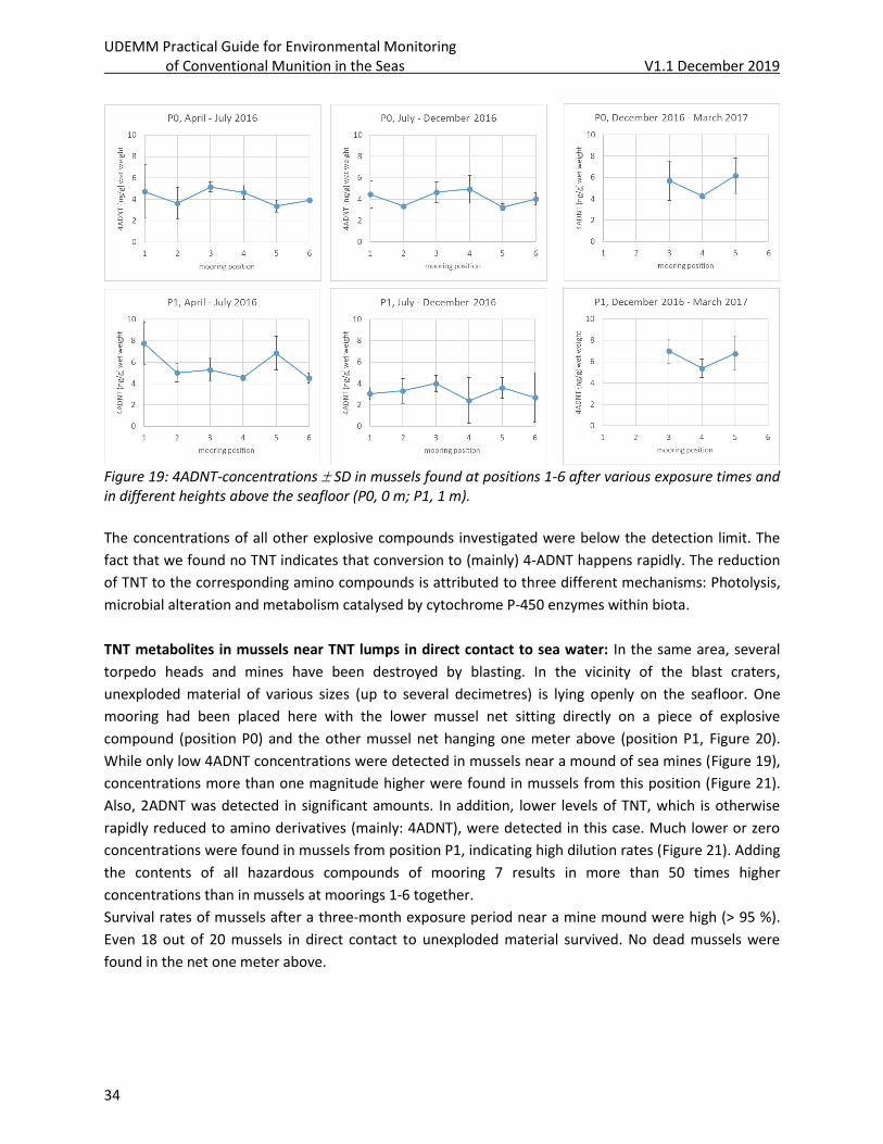
UDEMM Practical Guide for Environmental Monitoring of Conventional Munition in the Seas V1.1 December 2019
34
Figure 19: 4ADNT-concentrations SD in mussels found at positions 1-6 after various exposure times and in different heights above the seafloor (P0, 0 m; P1, 1 m).
The concentrations of all other explosive compounds investigated were below the detection limit. The
fact that we found no TNT indicates that conversion to (mainly) 4-ADNT happens rapidly. The reduction
of TNT to the corresponding amino compounds is attributed to three different mechanisms: Photolysis,
microbial alteration and metabolism catalysed by cytochrome P-450 enzymes within biota.
TNT metabolites in mussels near TNT lumps in direct contact to sea water: In the same area, several
torpedo heads and mines have been destroyed by blasting. In the vicinity of the blast craters,
unexploded material of various sizes (up to several decimetres) is lying openly on the seafloor. One
mooring had been placed here with the lower mussel net sitting directly on a piece of explosive
compound (position P0) and the other mussel net hanging one meter above (position P1, Figure 20).
While only low 4ADNT concentrations were detected in mussels near a mound of sea mines (Figure 19),
concentrations more than one magnitude higher were found in mussels from this position (Figure 21).
Also, 2ADNT was detected in significant amounts. In addition, lower levels of TNT, which is otherwise
rapidly reduced to amino derivatives (mainly: 4ADNT), were detected in this case. Much lower or zero
concentrations were found in mussels from position P1, indicating high dilution rates (Figure 21). Adding
the contents of all hazardous compounds of mooring 7 results in more than 50 times higher
concentrations than in mussels at moorings 1-6 together.
Survival rates of mussels after a three-month exposure period near a mine mound were high (> 95 %).
Even 18 out of 20 mussels in direct contact to unexploded material survived. No dead mussels were
found in the net one meter above.
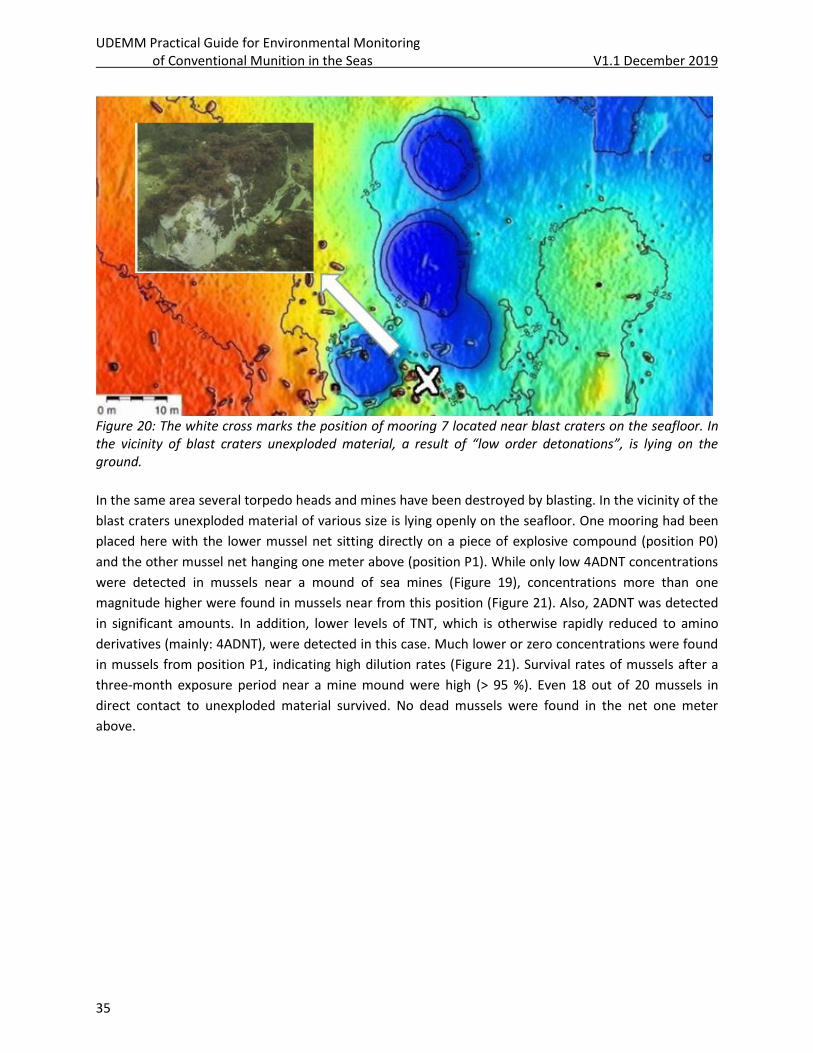
UDEMM Practical Guide for Environmental Monitoring of Conventional Munition in the Seas V1.1 December 2019
35
Figure 20: The white cross marks the position of mooring 7 located near blast craters on the seafloor. In the vicinity of blast craters unexploded material, a result of “low order detonations”, is lying on the ground.
In the same area several torpedo heads and mines have been destroyed by blasting. In the vicinity of the
blast craters unexploded material of various size is lying openly on the seafloor. One mooring had been
placed here with the lower mussel net sitting directly on a piece of explosive compound (position P0)
and the other mussel net hanging one meter above (position P1). While only low 4ADNT concentrations
were detected in mussels near a mound of sea mines (Figure 19), concentrations more than one
magnitude higher were found in mussels near from this position (Figure 21). Also, 2ADNT was detected
in significant amounts. In addition, lower levels of TNT, which is otherwise rapidly reduced to amino
derivatives (mainly: 4ADNT), were detected in this case. Much lower or zero concentrations were found
in mussels from position P1, indicating high dilution rates (Figure 21). Survival rates of mussels after a
three-month exposure period near a mine mound were high (> 95 %). Even 18 out of 20 mussels in
direct contact to unexploded material survived. No dead mussels were found in the net one meter
above.
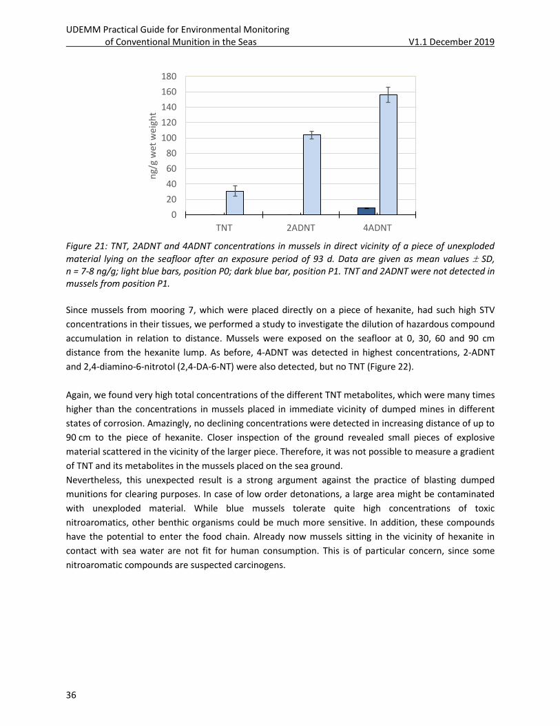
UDEMM Practical Guide for Environmental Monitoring of Conventional Munition in the Seas V1.1 December 2019
36
Figure 21: TNT, 2ADNT and 4ADNT concentrations in mussels in direct vicinity of a piece of unexploded
material lying on the seafloor after an exposure period of 93 d. Data are given as mean values SD, n = 7-8 ng/g; light blue bars, position P0; dark blue bar, position P1. TNT and 2ADNT were not detected in mussels from position P1.
Since mussels from mooring 7, which were placed directly on a piece of hexanite, had such high STV
concentrations in their tissues, we performed a study to investigate the dilution of hazardous compound
accumulation in relation to distance. Mussels were exposed on the seafloor at 0, 30, 60 and 90 cm
distance from the hexanite lump. As before, 4-ADNT was detected in highest concentrations, 2-ADNT
and 2,4-diamino-6-nitrotol (2,4-DA-6-NT) were also detected, but no TNT (Figure 22).
Again, we found very high total concentrations of the different TNT metabolites, which were many times
higher than the concentrations in mussels placed in immediate vicinity of dumped mines in different
states of corrosion. Amazingly, no declining concentrations were detected in increasing distance of up to
90 cm to the piece of hexanite. Closer inspection of the ground revealed small pieces of explosive
material scattered in the vicinity of the larger piece. Therefore, it was not possible to measure a gradient
of TNT and its metabolites in the mussels placed on the sea ground.
Nevertheless, this unexpected result is a strong argument against the practice of blasting dumped
munitions for clearing purposes. In case of low order detonations, a large area might be contaminated
with unexploded material. While blue mussels tolerate quite high concentrations of toxic
nitroaromatics, other benthic organisms could be much more sensitive. In addition, these compounds
have the potential to enter the food chain. Already now mussels sitting in the vicinity of hexanite in
contact with sea water are not fit for human consumption. This is of particular concern, since some
nitroaromatic compounds are suspected carcinogens.
0
20
40
60
80
100
120
140
160
180
TNT 2ADNT 4ADNT
ng/
g w
et w
eig
ht
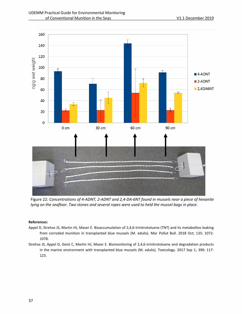
UDEMM Practical Guide for Environmental Monitoring of Conventional Munition in the Seas V1.1 December 2019
37
Figure 22: Concentrations of 4-ADNT, 2-ADNT and 2,4-DA-6NT found in mussels near a piece of hexanite lying on the seafloor. Two stones and several ropes were used to held the mussel bags in place.
References:
Appel D, Strehse JS, Martin HJ, Maser E. Bioaccumulation of 2,4,6-trinitrotoluene (TNT) and its metabolites leaking
from corroded munition in transplanted blue mussels (M. edulis). Mar Pollut Bull. 2018 Oct; 135: 1072-
1078.
Strehse JS, Appel D, Geist C, Martin HJ, Maser E. Biomonitoring of 2,4,6-trinitrotoluene and degradation products
in the marine environment with transplanted blue mussels (M. edulis). Toxicology. 2017 Sep 1; 390: 117-
123.
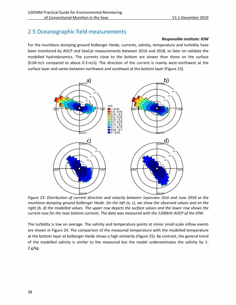
UDEMM Practical Guide for Environmental Monitoring of Conventional Munition in the Seas V1.1 December 2019
38
2.5 Oceanographic field measurements Responsible institute: IOW
For the munitions dumping ground Kolberger Heide, currents, salinity, temperature and turbidity have
been monitored by ADCP and SeaCat measurements between 2016 and 2018, to later on validate the
modelled hydrodynamics. The currents close to the bottom are slower than those on the surface
(0.04 m/s compared to about 0.3 m/s). The direction of the current is mainly west-northwest at the
surface layer and varies between northwest and southeast at the bottom layer (Figure 23).
Figure 23: Distribution of current direction and velocity between September 2016 and June 2018 at the munitions dumping ground Kolberger Heide. On the left (a, c), we show the observed values and on the right (b, d) the modelled values. The upper row depicts the surface values and the lower row shows the current rose for the near bottom currents. The data was measured with the 1200kHz ADCP of the IOW.
The turbidity is low on average. The salinity and temperature points at minor small-scale inflow events
are shown in Figure 24. The comparison of the measured temperature with the modelled temperature
at the bottom layer at Kolberger Heide shows a high similarity (Figure 25). By contrast, the general trend
of the modelled salinity is similar to the measured but the model underestimates the salinity by 1-
2 g/kg.
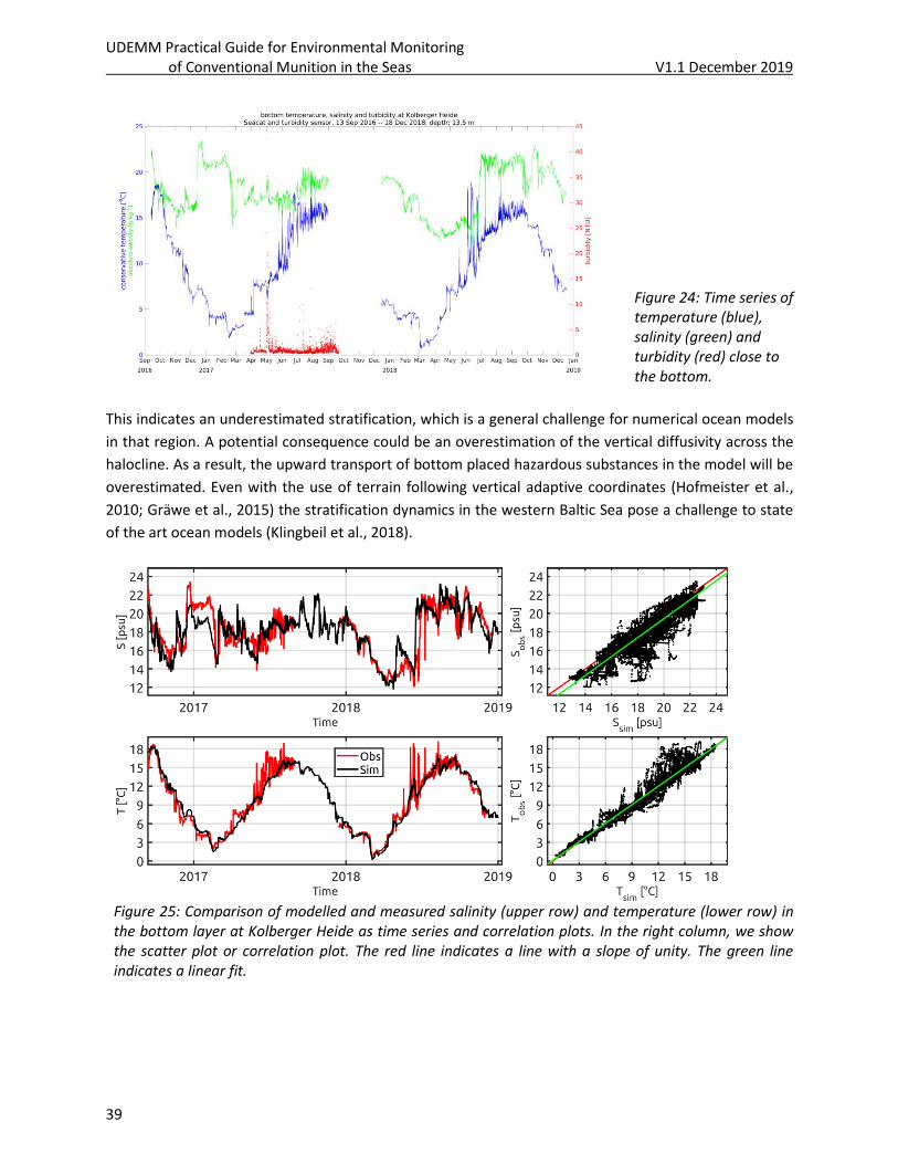
UDEMM Practical Guide for Environmental Monitoring of Conventional Munition in the Seas V1.1 December 2019
39
Figure 24: Time series of temperature (blue), salinity (green) and turbidity (red) close to the bottom.
This indicates an underestimated stratification, which is a general challenge for numerical ocean models
in that region. A potential consequence could be an overestimation of the vertical diffusivity across the
halocline. As a result, the upward transport of bottom placed hazardous substances in the model will be
overestimated. Even with the use of terrain following vertical adaptive coordinates (Hofmeister et al.,
2010; Gräwe et al., 2015) the stratification dynamics in the western Baltic Sea pose a challenge to state
of the art ocean models (Klingbeil et al., 2018).
Figure 25: Comparison of modelled and measured salinity (upper row) and temperature (lower row) in the bottom layer at Kolberger Heide as time series and correlation plots. In the right column, we show the scatter plot or correlation plot. The red line indicates a line with a slope of unity. The green line indicates a linear fit.
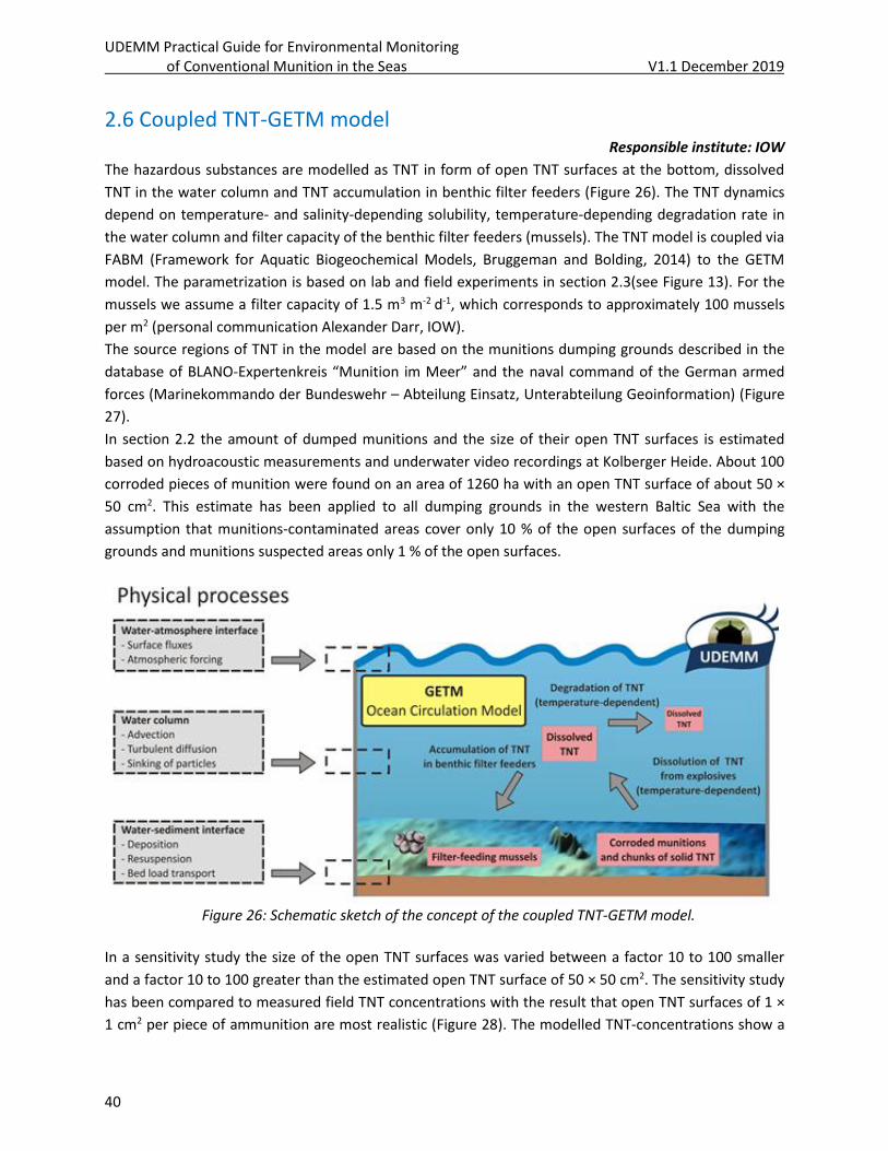
UDEMM Practical Guide for Environmental Monitoring of Conventional Munition in the Seas V1.1 December 2019
40
2.6 Coupled TNT-GETM model Responsible institute: IOW
The hazardous substances are modelled as TNT in form of open TNT surfaces at the bottom, dissolved
TNT in the water column and TNT accumulation in benthic filter feeders (Figure 26). The TNT dynamics
depend on temperature- and salinity-depending solubility, temperature-depending degradation rate in
the water column and filter capacity of the benthic filter feeders (mussels). The TNT model is coupled via
FABM (Framework for Aquatic Biogeochemical Models, Bruggeman and Bolding, 2014) to the GETM
model. The parametrization is based on lab and field experiments in section 2.3(see Figure 13). For the
mussels we assume a filter capacity of 1.5 m3 m-2 d-1, which corresponds to approximately 100 mussels
per m2 (personal communication Alexander Darr, IOW).
The source regions of TNT in the model are based on the munitions dumping grounds described in the
database of BLANO-Expertenkreis “Munition im Meer” and the naval command of the German armed
forces (Marinekommando der Bundeswehr – Abteilung Einsatz, Unterabteilung Geoinformation) (Figure
27).
In section 2.2 the amount of dumped munitions and the size of their open TNT surfaces is estimated
based on hydroacoustic measurements and underwater video recordings at Kolberger Heide. About 100
corroded pieces of munition were found on an area of 1260 ha with an open TNT surface of about 50 ×
50 cm2. This estimate has been applied to all dumping grounds in the western Baltic Sea with the
assumption that munitions-contaminated areas cover only 10 % of the open surfaces of the dumping
grounds and munitions suspected areas only 1 % of the open surfaces.
Figure 26: Schematic sketch of the concept of the coupled TNT-GETM model.
In a sensitivity study the size of the open TNT surfaces was varied between a factor 10 to 100 smaller
and a factor 10 to 100 greater than the estimated open TNT surface of 50 × 50 cm2. The sensitivity study
has been compared to measured field TNT concentrations with the result that open TNT surfaces of 1 ×
1 cm2 per piece of ammunition are most realistic (Figure 28). The modelled TNT-concentrations show a
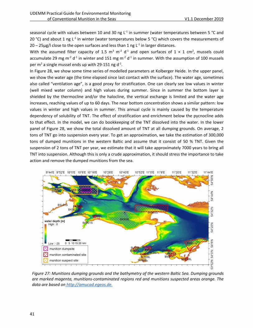
UDEMM Practical Guide for Environmental Monitoring of Conventional Munition in the Seas V1.1 December 2019
41
seasonal cycle with values between 10 and 30 ng L-1 in summer (water temperatures between 5 °C and
20 °C) and about 1 ng L-1 in winter (water temperatures below 5 °C) which covers the measurements of
20 – 25µg/l close to the open surfaces and less than 1 ng L-1 in larger distances.
With the assumed filter capacity of 1.5 m3 m-2 d-1 and open surfaces of 1 × 1 cm2, mussels could
accumulate 29 mg m-2 d-1 in winter and 151 mg m-2 d-1 in summer. With the assumption of 100 mussels
per m2 a single mussel ends up with 29-151 ng d-1.
In Figure 28, we show some time series of modelled parameters at Kolberger Heide. In the upper panel,
we show the water age (the time elapsed since last contact with the surface). The water age, sometimes
also called “ventilation age”, is a good proxy for stratification. One can clearly see low values in winter
(well mixed water column) and high values during summer. Since in summer the bottom layer is
shielded by the thermocline and/or the halocline, the vertical exchange is limited and the water age
increases, reaching values of up to 60 days. The near bottom concentration shows a similar pattern: low
values in winter and high values in summer. This annual cycle is mainly caused by the temperature
dependency of solubility of TNT. The effect of stratification and enrichment below the pycnocline adds
to that effect. In the model, we can do bookkeeping of the TNT dissolved into the water. In the lower
panel of Figure 28, we show the total dissolved amount of TNT at all dumping grounds. On average, 2
tons of TNT go into suspension every year. To get an approximation, we take the estimation of 300,000
tons of dumped munitions in the western Baltic and assume that it consist of 50 % TNT. Given the
suspension of 2 tons of TNT per year, we estimate that it will take approximately 7000 years to bring all
TNT into suspension. Although this is only a crude approximation, it should stress the importance to take
action and remove the dumped munitions from the sea.
Figure 27: Munitions dumping grounds and the bathymetry of the western Baltic Sea. Dumping grounds are marked magenta, munitions-contaminated regions red and munitions suspected areas orange. The data are based on http://amucad.egeos.de.
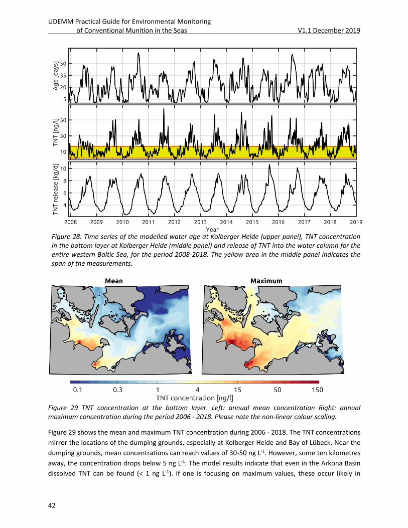
UDEMM Practical Guide for Environmental Monitoring of Conventional Munition in the Seas V1.1 December 2019
42
Figure 28: Time series of the modelled water age at Kolberger Heide (upper panel), TNT concentration in the bottom layer at Kolberger Heide (middle panel) and release of TNT into the water column for the entire western Baltic Sea, for the period 2008-2018. The yellow area in the middle panel indicates the span of the measurements.
Figure 29 TNT concentration at the bottom layer. Left: annual mean concentration Right: annual maximum concentration during the period 2006 - 2018. Please note the non-linear colour scaling.
Figure 29 shows the mean and maximum TNT concentration during 2006 - 2018. The TNT concentrations
mirror the locations of the dumping grounds, especially at Kolberger Heide and Bay of Lübeck. Near the
dumping grounds, mean concentrations can reach values of 30-50 ng L-1. However, some ten kilometres
away, the concentration drops below 5 ng L-1. The model results indicate that even in the Arkona Basin
dissolved TNT can be found (< 1 ng L-1). If one is focusing on maximum values, these occur likely in
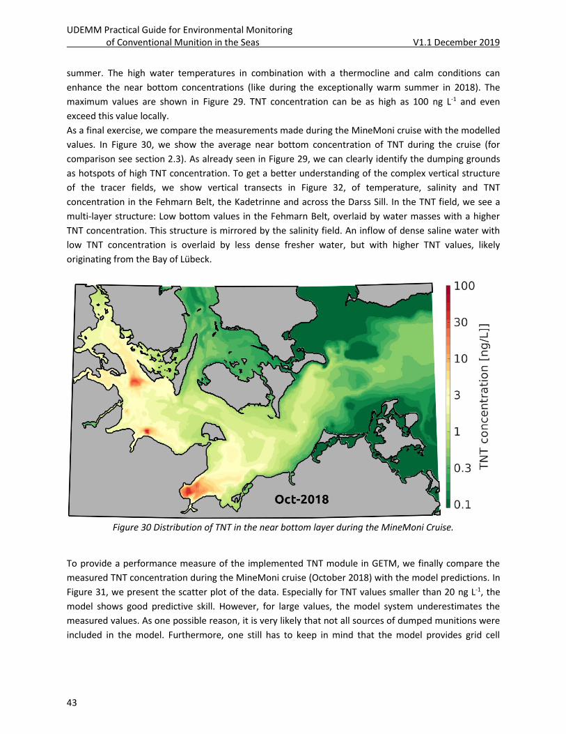
UDEMM Practical Guide for Environmental Monitoring of Conventional Munition in the Seas V1.1 December 2019
43
summer. The high water temperatures in combination with a thermocline and calm conditions can
enhance the near bottom concentrations (like during the exceptionally warm summer in 2018). The
maximum values are shown in Figure 29. TNT concentration can be as high as 100 ng L-1 and even
exceed this value locally.
As a final exercise, we compare the measurements made during the MineMoni cruise with the modelled
values. In Figure 30, we show the average near bottom concentration of TNT during the cruise (for
comparison see section 2.3). As already seen in Figure 29, we can clearly identify the dumping grounds
as hotspots of high TNT concentration. To get a better understanding of the complex vertical structure
of the tracer fields, we show vertical transects in Figure 32, of temperature, salinity and TNT
concentration in the Fehmarn Belt, the Kadetrinne and across the Darss Sill. In the TNT field, we see a
multi-layer structure: Low bottom values in the Fehmarn Belt, overlaid by water masses with a higher
TNT concentration. This structure is mirrored by the salinity field. An inflow of dense saline water with
low TNT concentration is overlaid by less dense fresher water, but with higher TNT values, likely
originating from the Bay of Lübeck.
Figure 30 Distribution of TNT in the near bottom layer during the MineMoni Cruise.
To provide a performance measure of the implemented TNT module in GETM, we finally compare the
measured TNT concentration during the MineMoni cruise (October 2018) with the model predictions. In
Figure 31, we present the scatter plot of the data. Especially for TNT values smaller than 20 ng L-1, the
model shows good predictive skill. However, for large values, the model system underestimates the
measured values. As one possible reason, it is very likely that not all sources of dumped munitions were
included in the model. Furthermore, one still has to keep in mind that the model provides grid cell
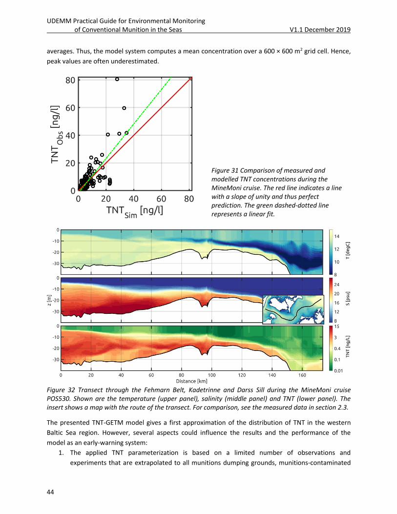
UDEMM Practical Guide for Environmental Monitoring of Conventional Munition in the Seas V1.1 December 2019
44
averages. Thus, the model system computes a mean concentration over a 600 × 600 m2 grid cell. Hence,
peak values are often underestimated.
Figure 31 Comparison of measured and modelled TNT concentrations during the MineMoni cruise. The red line indicates a line with a slope of unity and thus perfect prediction. The green dashed-dotted line represents a linear fit.
Figure 32 Transect through the Fehmarn Belt, Kadetrinne and Darss Sill during the MineMoni cruise POS530. Shown are the temperature (upper panel), salinity (middle panel) and TNT (lower panel). The insert shows a map with the route of the transect. For comparison, see the measured data in section 2.3.
The presented TNT-GETM model gives a first approximation of the distribution of TNT in the western
Baltic Sea region. However, several aspects could influence the results and the performance of the
model as an early-warning system:
1. The applied TNT parameterization is based on a limited number of observations and
experiments that are extrapolated to all munitions dumping grounds, munitions-contaminated
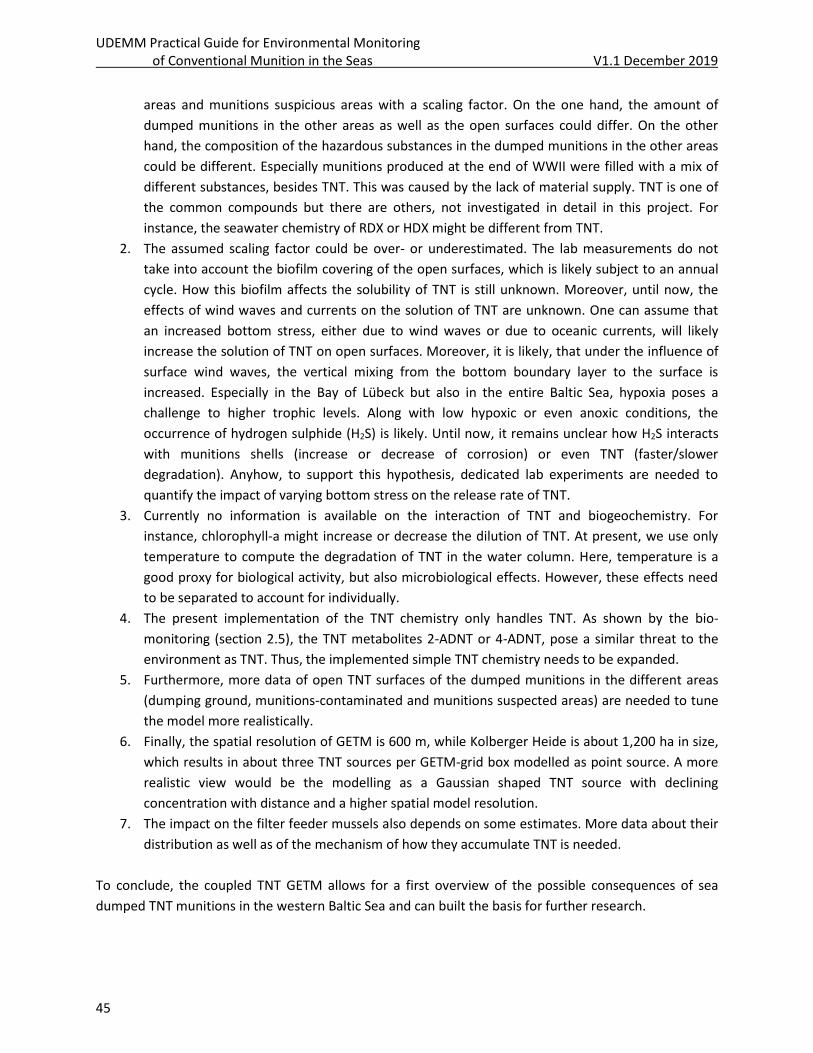
UDEMM Practical Guide for Environmental Monitoring of Conventional Munition in the Seas V1.1 December 2019
45
areas and munitions suspicious areas with a scaling factor. On the one hand, the amount of
dumped munitions in the other areas as well as the open surfaces could differ. On the other
hand, the composition of the hazardous substances in the dumped munitions in the other areas
could be different. Especially munitions produced at the end of WWII were filled with a mix of
different substances, besides TNT. This was caused by the lack of material supply. TNT is one of
the common compounds but there are others, not investigated in detail in this project. For
instance, the seawater chemistry of RDX or HDX might be different from TNT.
2. The assumed scaling factor could be over- or underestimated. The lab measurements do not
take into account the biofilm covering of the open surfaces, which is likely subject to an annual
cycle. How this biofilm affects the solubility of TNT is still unknown. Moreover, until now, the
effects of wind waves and currents on the solution of TNT are unknown. One can assume that
an increased bottom stress, either due to wind waves or due to oceanic currents, will likely
increase the solution of TNT on open surfaces. Moreover, it is likely, that under the influence of
surface wind waves, the vertical mixing from the bottom boundary layer to the surface is
increased. Especially in the Bay of Lübeck but also in the entire Baltic Sea, hypoxia poses a
challenge to higher trophic levels. Along with low hypoxic or even anoxic conditions, the
occurrence of hydrogen sulphide (H2S) is likely. Until now, it remains unclear how H2S interacts
with munitions shells (increase or decrease of corrosion) or even TNT (faster/slower
degradation). Anyhow, to support this hypothesis, dedicated lab experiments are needed to
quantify the impact of varying bottom stress on the release rate of TNT.
3. Currently no information is available on the interaction of TNT and biogeochemistry. For
instance, chlorophyll-a might increase or decrease the dilution of TNT. At present, we use only
temperature to compute the degradation of TNT in the water column. Here, temperature is a
good proxy for biological activity, but also microbiological effects. However, these effects need
to be separated to account for individually.
4. The present implementation of the TNT chemistry only handles TNT. As shown by the bio-
monitoring (section 2.5), the TNT metabolites 2-ADNT or 4-ADNT, pose a similar threat to the
environment as TNT. Thus, the implemented simple TNT chemistry needs to be expanded.
5. Furthermore, more data of open TNT surfaces of the dumped munitions in the different areas
(dumping ground, munitions-contaminated and munitions suspected areas) are needed to tune
the model more realistically.
6. Finally, the spatial resolution of GETM is 600 m, while Kolberger Heide is about 1,200 ha in size,
which results in about three TNT sources per GETM-grid box modelled as point source. A more
realistic view would be the modelling as a Gaussian shaped TNT source with declining
concentration with distance and a higher spatial model resolution.
7. The impact on the filter feeder mussels also depends on some estimates. More data about their
distribution as well as of the mechanism of how they accumulate TNT is needed.
To conclude, the coupled TNT GETM allows for a first overview of the possible consequences of sea
dumped TNT munitions in the western Baltic Sea and can built the basis for further research.
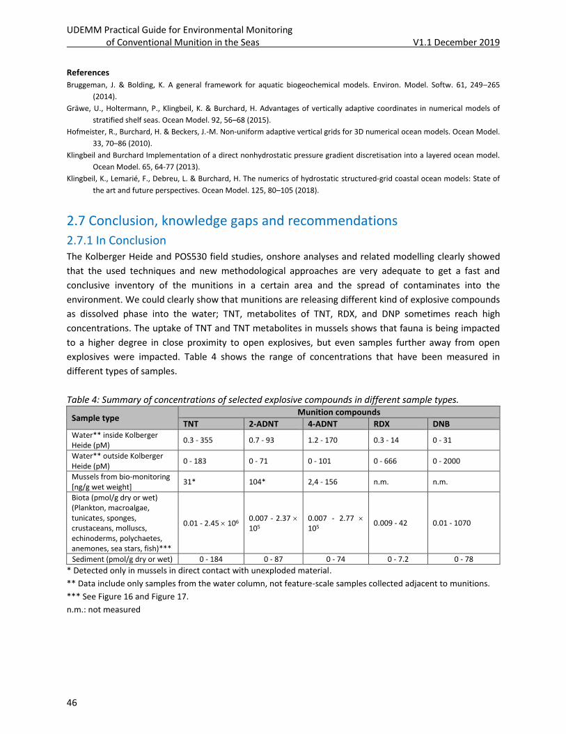
UDEMM Practical Guide for Environmental Monitoring of Conventional Munition in the Seas V1.1 December 2019
46
References
Bruggeman, J. & Bolding, K. A general framework for aquatic biogeochemical models. Environ. Model. Softw. 61, 249–265
(2014).
Gräwe, U., Holtermann, P., Klingbeil, K. & Burchard, H. Advantages of vertically adaptive coordinates in numerical models of
stratified shelf seas. Ocean Model. 92, 56–68 (2015).
Hofmeister, R., Burchard, H. & Beckers, J.-M. Non-uniform adaptive vertical grids for 3D numerical ocean models. Ocean Model.
33, 70–86 (2010).
Klingbeil and Burchard Implementation of a direct nonhydrostatic pressure gradient discretisation into a layered ocean model.
Ocean Model. 65, 64-77 (2013).
Klingbeil, K., Lemarié, F., Debreu, L. & Burchard, H. The numerics of hydrostatic structured-grid coastal ocean models: State of
the art and future perspectives. Ocean Model. 125, 80–105 (2018).
2.7 Conclusion, knowledge gaps and recommendations
2.7.1 In Conclusion The Kolberger Heide and POS530 field studies, onshore analyses and related modelling clearly showed
that the used techniques and new methodological approaches are very adequate to get a fast and
conclusive inventory of the munitions in a certain area and the spread of contaminates into the
environment. We could clearly show that munitions are releasing different kind of explosive compounds
as dissolved phase into the water; TNT, metabolites of TNT, RDX, and DNP sometimes reach high
concentrations. The uptake of TNT and TNT metabolites in mussels shows that fauna is being impacted
to a higher degree in close proximity to open explosives, but even samples further away from open
explosives were impacted. Table 4 shows the range of concentrations that have been measured in
different types of samples.
Table 4: Summary of concentrations of selected explosive compounds in different sample types.
Sample type Munition compounds
TNT 2-ADNT 4-ADNT RDX DNB Water** inside Kolberger Heide (pM)
0.3 - 355 0.7 - 93 1.2 - 170 0.3 - 14 0 - 31
Water** outside Kolberger Heide (pM)
0 - 183 0 - 71 0 - 101 0 - 666 0 - 2000
Mussels from bio-monitoring [ng/g wet weight]
31* 104* 2,4 - 156 n.m. n.m.
Biota (pmol/g dry or wet) (Plankton, macroalgae, tunicates, sponges, crustaceans, molluscs, echinoderms, polychaetes, anemones, sea stars, fish)***
0.01 - 2.45 106 0.007 - 2.37 105
0.007 - 2.77 105
0.009 - 42 0.01 - 1070
Sediment (pmol/g dry or wet) 0 - 184 0 - 87 0 - 74 0 - 7.2 0 - 78
* Detected only in mussels in direct contact with unexploded material.
** Data include only samples from the water column, not feature-scale samples collected adjacent to munitions.
*** See Figure 16 and Figure 17.
n.m.: not measured
UDEMM Practical Guide for Environmental Monitoring of Conventional Munition in the Seas V1.1 December 2019
47
2.7.2 Knowledge gaps Knowledge gaps have been identified by the UDEMM consortium. This non- complete list is presented to
highlight the topics and detailed needs to better understand the impact of marine munitions on the
environment. We regard all of them as being important enough to be part of upcoming monitoring and
particularly future financed research. They are grouped in different scientific disciplines.
Archive investigation knowledge gaps:
Extensive work has been done but massive amounts of archive documents still need to be carefully
examined. Methods such as digital text recognition and machine learning could enhance the process and
help with the identification and connection of information. This will lead to a more precise knowledge
on the number of ammunition objects dumped into the sea and a better identification of so far
unknown hot spots.
Physical knowledge gaps:
Environmental controls on munitions housing corrosion: Corrosion was not addressed in UDEMM.TNT
release and distribution primarily depends on the source strength. The strength of this source depends
on the corrosion state and exposure of the explosives to seawater. Environmental factors such as
salinity and dissolved oxygen may affect corrosion rates, and most likely vary throughout the Baltic Sea.
Effect of sedimentological processes on munitions deposition: Sediment scours can form around
ammunition objects due to water currents or waves initiating object displacement and burial. These
processes are complex and coupled to sediment composition, slope, water depth, object shape and
incident burial depth. Numerical models are still not able to include all parameters and therefore scour
formation, as well as subsequent displacement and burial cannot be reliably predicted. Also the effect of
vegetation overgrowth of objects on the fluid dynamic around the object and its influence on mixed
grain size distributions need to be addressed to generate a good predictive numerical model on
munitions re-deposition and long-term dumping ground stability.
Influence of hydrodynamic forces (current or wave induced) on TNT solubility and spreading: The
influence of hydrodynamic forces acting on exposed explosives might increase their mechanic erosion
and enhance solubility. Such processes should be incorporated into chemical models for predicting
mixing and dissolution rates. Mechanical weathering and erosion of exposed explosives will modulate
MC spreading and environmental contamination.
Chemical knowledge gaps:
Mixing energy effects on explosive dissolution rates: Results of laboratory and in situ dissolution
experiments in UDEMM indicated low release rates and suggest that mixing energy may be the primary
control on TNT dissolution rate. Regional differences or changes in waves and currents may therefore
have a major effect on MC release from underwater munitions.
Effect of climate change on munitions and contaminant release: Climate change effects include
increasing temperature, decreasing pH, and increasing intensity of storms. These changes will impact
the rate of corrosion, chemical release, and movement of underwater munitions. Additional work on the
UDEMM Practical Guide for Environmental Monitoring of Conventional Munition in the Seas V1.1 December 2019
48
relevant parameters will allow evaluating the climate induced consequences of MC release. Potential
effects could already be tested with the oceanographic model developed in UDEMM.
Microbial and physicochemical degradation in relation to time and environmental parameters: The
good match between measured and modelled TNT concentrations including microbial TNT
transformation suggests that microbial activity is indeed a major control on the fate of TNT in the
bottom water. More research is needed to evaluate the strong temperature dependence of microbial
activity but at the same time quantify the sunlight effect on TNT transformation in surface waters. The
effect of decreased oxygen concentrations (and dissolved sulphides) during hypoxia events may also be
an important factor as some TNT transformation pathways occur only under strictly anoxic conditions.
Importance of MC mineralization vs transformation: Transformation products of TNT (ADNT, DANT)
were identified to be important components of MC contamination in the environment. These daughter-
compounds, as well as others, can be equally toxic as or more toxic than the parent compound.
Quantitative mass balance analyses for MCs released from underwater munitions are important to
understand the extent to which contaminants are removed from the environment (i.e., degraded to
inorganic constituent compounds) or simply transformed to other forms.
Biological and toxicological knowledge gaps:
Pathways of contaminant accumulation in and out of the biota: MCs were measured in different
organisms found in place and accumulation was observed in mussels deployed for biomonitoring.
Questions still remain, if organisms accumulate MCs from the dissolved phase, particulate food they
ingest (including particulate MCs) or both. It is important to determine the partitioning of MCs in
different body tissues, particularly in relevant seafood organisms. Also the effect of potentially
decreasing contaminant levels within organisms should be determined, to establish if contaminants can
be fully degraded or ‘flushed’ from the organism.
MCs accumulation in food webs and human seafood: MCs were measured in UDEMM in a limited
number of organisms throughout the food web, including seafood species. A systematic and statistically
robust investigation is necessary to determine, whether MCs are transferred among trophic levels, and
the extent to which commercial seafood is affected by environmental MC contamination already.
DMM as habitats: Ammunition objects provide hard substrate and shelter for sessile biota and actually
act as artificial habitats and reefs. Since marine flora and fauna particularly live in such environments, a
systematic comparison of dumping ground with uncontaminated marine habitats of very similar type is
important to determine the importance of dumping ground as local ecosystems.
MCs as part of a multi-stressor environment: Marine organisms are exposed to a number of stressors,
which influence their reproduction rate and fitness. Assuming that MCs do accumulate within marine
organisms and do have a certain toxicity, it is important to analyse the role of these contaminants as
part of the multi-stressor environment for individual groups of organisms. Effects of TNT on fish health
might be e.g. smaller or greater compared to a parallel uptake of e.g. heavy metals like mercury. It might
also be possible that negative effects of other stressors can be enhanced, when MC uptake is increased.
A clear understanding of MCs on the organism health in a multi-stressor environment needs to be
known.
Toxicity of different MCs: Toxicity levels for all MCs and its degradation products need to be
established. This way, human seafood can be evaluated to be toxic or not more easily and
UDEMM Practical Guide for Environmental Monitoring of Conventional Munition in the Seas V1.1 December 2019
49
recommendations can be given. The establishment of proper toxicity levels is the base for any
recommendation to restrict seafood consumption or to close fishing grounds.
Monitoring knowledge gaps:
Spatial and temporal patterns observed in UDEMM and replicated in the computer model revealed
widespread and seasonally-variable transport of MCs. Long-term monitoring at munitions hotspots and
control sites is necessary to evaluate the persistence of these trends, and the extent to which hotspots
differ from un-impacted locations.
Methodological knowledge gaps:
Validation and inter-comparison of analytical methods: Two analytical methods were used in UDEMM
(GC-MS and LC-MS), but many others exist. It is critical to validate and ground truth these different
methods. Intercomparison/intercalibration experiments are essential, as is the development of
reference materials for water, sediment and biota.
Autonomous munitions detection: Depending on ammunition type and environment, different
detection methods exist but typically a combination of different methods and validation via divers is
needed. This requires extensive ship time and man power. Artificial intelligence could combine different
methods in an objective way, even online, while data are still acquired. This would improve munitions
detection and could allow setting standards for munitions detection and the clearance of areas. Several
AUV platforms can be operated in parallel, which would reduce time and costs of surveying for UXO
removal and environmental monitoring purposes alike.
2.7.3 Recommendation We recommend overcoming political, administrative and technical problems for a better integrative
data management of all relevant data. We propose to establish a federated data infrastructure with
different access levels that allow viewing general information about munitions in the sea all the way to
very detailed and restricted information such as exact munitions locations, planned disposal actions and
plans for intervention. Data of public interest such as concentrations in the water column and fish
should be presented openly with automatic updates originating from latest measurements.
Linked to data management concerns (standardisation) but also to keep comparability of measurements
high, we recommend that MC data in environmental samples be reported in molar units (e.g. pM,
picomole per litre; pmol/g, picomole per gram sediment or tissue) rather than mass units. This allows
direct comparison among the parent and transformation products. For example, complete
transformation of one pmol TNT produces 1 pmol ADNT, and eventually 1 pmol DANT. In contrast,
transformation of 1 ng TNT produces 0.86 ng of ADNT and 0.74 ng of DANT. Two exceptions to this
recommendation are when reporting measurements or rates of explosive solid dissolution and tissue
concentrations for toxicological risk analysis. In the case of explosive solid dissolution, mass units
provide a more direct relationship with solid loss, (i.e. in relation to explosive volume and density). In
addition, reporting MC data in biota in mass units (e.g. picogram per gram dry weight or per gram wet
weight) allows comparisons with toxicological limit values (e.g. maximum residue levels in food). Molar
masses for the MCs reported in this document and unit conversions are listed in Table 5.
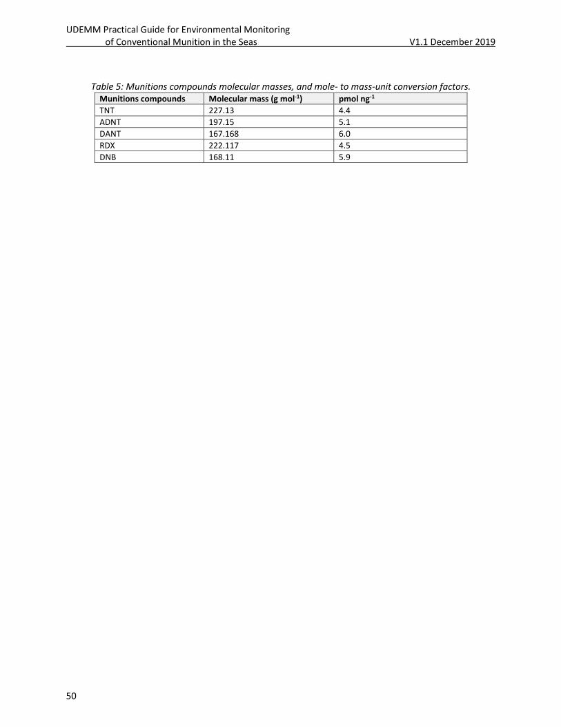
UDEMM Practical Guide for Environmental Monitoring of Conventional Munition in the Seas V1.1 December 2019
50
Table 5: Munitions compounds molecular masses, and mole- to mass-unit conversion factors. Munitions compounds Molecular mass (g mol-1) pmol ng-1
TNT 227.13 4.4
ADNT 197.15 5.1
DANT 167.168 6.0
RDX 222.117 4.5
DNB 168.11 5.9
UDEMM Practical Guide for Environmental Monitoring of Conventional Munition in the Seas V1.1 December 2019
51
3. Practical guidence for sampling and monitoring
3.1 Scientifically “best” monitoring This section describes the our scientifically ‘best practice’ for sampling and monitoring munitions-
contaminated areas in seas and oceans. This means that to our current knowledge the presented
methods and approaches allow for a detailed assessment and the evaluation of the state of the
environment. The acquired data are furthermore important for a long-term monitoring approach and
allow for adjustments and refinements at any time. Generally, the ‘best’ monitoring should start as soon
as possible, meaning starting monitoring NOW, and runs for a sufficient amount of time after which it
can be assumed that no additional contamination will occur anymore. Based on our results and model
based extrapolations we see a minimum time for monitoring to be AT LEAST for 30 years from now.
Three main purposes are seen for the monitoring, including the baseline study, the long-term
monitoring and a short term ad-hoc monitoring that should take place before, during and after
clearance and here particularly during blast-in-place operations. The baseline study should include a
good knowledge about the history of the munitions dumping ground from historic records, to answer
the questions of what types of munitions is present and what kinds of explosives are likely to be
dominant. The baseline study should further include a habitat characterization as this will determine the
needed/useful sampling (e.g. geophysical methods as sub-bottom profiling/electro-magnetic) and
monitoring methods (e.g. biomonitoring through mussels and/or fish or the use of passive samplers
instead). Already first results of the initial mapping will allow determining the size of the area that is
contaminated and thus needs to be surveyed in detail. Not included in this guide are recommendations
for sub-bottom mapping with acoustic and electro-magnetic sensors as these were not part of the
UDEMM sensor portfolio. A respective knowledge about suitable systems, their application, processing
and interpretation already exists in UXO survey and clearance companies(Frey et al., 2019).
Recommendations for monitoring chemical warfare dumpsites have been released by the NATO project
MODUM (Bełdowski et al., 2018) and incorporate the need of baseline studies for an area wide
assessment and resulting selection of sepcific areas of interest. These recommendations can be adapted
to conventional dumpsites. As highlighted in the chapters before, baseline studies need to include
oceanographic and chemical studies of the water column with both types of investigations going hand in
hand for a scientifically sound and meaningful data acquisition. Ideally, a well-established and validated
oceanographic model supports these studies and is fully integrated in any risk assessment and
prediction. All long-term monitoring builds on the comparison of data that have been acquired over long
time with different sensors measuring the same parameter, with different analytical methodologies that
over the time will become more accurate and with ever higher resolving acoustic and optical systems. A
good and sustainable data management is thus of utmost importance with ideally one authority
collecting, hosting and maintaining the respective data base.
How to prioritize the order in which specific areas will be monitored next, depends on several factors,
including e.g. a) the amount of open explosives being in direct contact with water and thus are the
strongest contamination hot spot, b) the need for underwater installations in a specific area, or c) ad-
hoc observations before clearance. In all cases monitoring needs to be adjusted specifically to the spatial
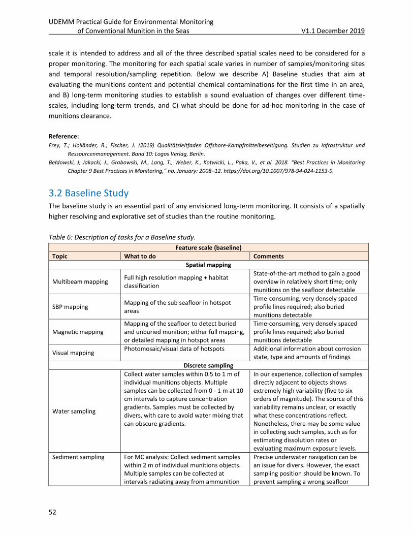
UDEMM Practical Guide for Environmental Monitoring of Conventional Munition in the Seas V1.1 December 2019
52
scale it is intended to address and all of the three described spatial scales need to be considered for a
proper monitoring. The monitoring for each spatial scale varies in number of samples/monitoring sites
and temporal resolution/sampling repetition. Below we describe A) Baseline studies that aim at
evaluating the munitions content and potential chemical contaminations for the first time in an area,
and B) long-term monitoring studies to establish a sound evaluation of changes over different time-
scales, including long-term trends, and C) what should be done for ad-hoc monitoring in the case of
munitions clearance.
Reference:
Frey, T.; Holländer, R.; Fischer, J. (2019) Qualitätsleitfaden Offshore-Kampfmittelbeseitigung. Studien zu Infrastruktur und
Ressourcenmanagement. Band 10: Logos Verlag, Berlin.
Bełdowski, J, Jakacki, J., Grabowski, M., Lang, T., Weber, K., Kotwicki, L., Paka, V., et al. 2018. “Best Practices in Monitoring
Chapter 9 Best Practices in Monitoring,” no. January: 2008–12. https://doi.org/10.1007/978-94-024-1153-9.
3.2 Baseline Study The baseline study is an essential part of any envisioned long-term monitoring. It consists of a spatially
higher resolving and explorative set of studies than the routine monitoring.
Table 6: Description of tasks for a Baseline study.
Feature scale (baseline)
Topic What to do Comments
Spatial mapping
Multibeam mapping Full high resolution mapping + habitat classification
State-of-the-art method to gain a good overview in relatively short time; only munitions on the seafloor detectable
SBP mapping Mapping of the sub seafloor in hotspot areas
Time-consuming, very densely spaced profile lines required; also buried munitions detectable
Magnetic mapping Mapping of the seafloor to detect buried and unburied munition; either full mapping, or detailed mapping in hotspot areas
Time-consuming, very densely spaced profile lines required; also buried munitions detectable
Visual mapping Photomosaic/visual data of hotspots Additional information about corrosion
state, type and amounts of findings
Discrete sampling
Water sampling
Collect water samples within 0.5 to 1 m of individual munitions objects. Multiple samples can be collected from 0 - 1 m at 10 cm intervals to capture concentration gradients. Samples must be collected by divers, with care to avoid water mixing that can obscure gradients.
In our experience, collection of samples directly adjacent to objects shows extremely high variability (five to six orders of magnitude). The source of this variability remains unclear, or exactly what these concentrations reflect. Nonetheless, there may be some value in collecting such samples, such as for estimating dissolution rates or evaluating maximum exposure levels.
Sediment sampling For MC analysis: Collect sediment samples within 2 m of individual munitions objects. Multiple samples can be collected at intervals radiating away from ammunition
Precise underwater navigation can be an issue for divers. However, the exact sampling position should be known. To prevent sampling a wrong seafloor
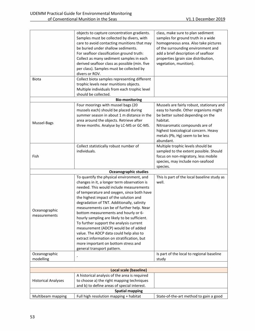
UDEMM Practical Guide for Environmental Monitoring of Conventional Munition in the Seas V1.1 December 2019
53
objects to capture concentration gradients. Samples must be collected by divers, with care to avoid contacting munitions that may be buried under shallow sediments. For seafloor classification ground truth: Collect as many sediment samples in each derived seafloor class as possible (min. five per class). Samples must be collected by divers or ROV.
class, make sure to plan sediment samples for ground truth in a wide homogeneous area. Also take pictures of the surrounding environment and add a brief description of seafloor properties (grain size distribution, vegetation, munition).
Biota Collect biota samples representing different trophic levels near munitions objects. Multiple individuals from each trophic level should be collected.
Bio-monitoring
Mussel-Bags
Four moorings with mussel bags (20 mussels each) should be placed during summer season in about 1 m distance in the area around the objects. Retrieve after three months. Analyse by LC-MS or GC-MS.
Mussels are fairly robust, stationary and easy to handle. Other organisms might be better suited depending on the habitat. Nitroaromatic compounds are of highest toxicological concern. Heavy metals (Pb, Hg) seem to be less abundant.
Fish
Collect statistically robust number of individuals.
Multiple trophic levels should be sampled to the extent possible. Should focus on non-migratory, less mobile species, may include non-seafood species.
Oceanographic studies
Oceanographic measurements
To quantify the physical environment, and changes in it, a longer term observation is needed. This would include measurements of temperature and oxygen, since both have the highest impact of the solution and degradation of TNT. Additionally, salinity measurements can be of further help. Near bottom measurements and hourly or 6-hourly sampling are likely to be sufficient. To further support the analysis current measurement (ADCP) would be of added value. The ADCP data could help also to extract information on stratification, but more important on bottom stress and general transport pattern.
This Is part of the local baseline study as well.
Oceanographic modelling
- Is part of the local to regional baseline study
Local scale (baseline)
Historical Analyses A historical analysis of the area is required to choose a) the right mapping techniques and b) to define areas of special interest.
Spatial mapping
Multibeam mapping Full high resolution mapping + habitat State-of-the-art method to gain a good
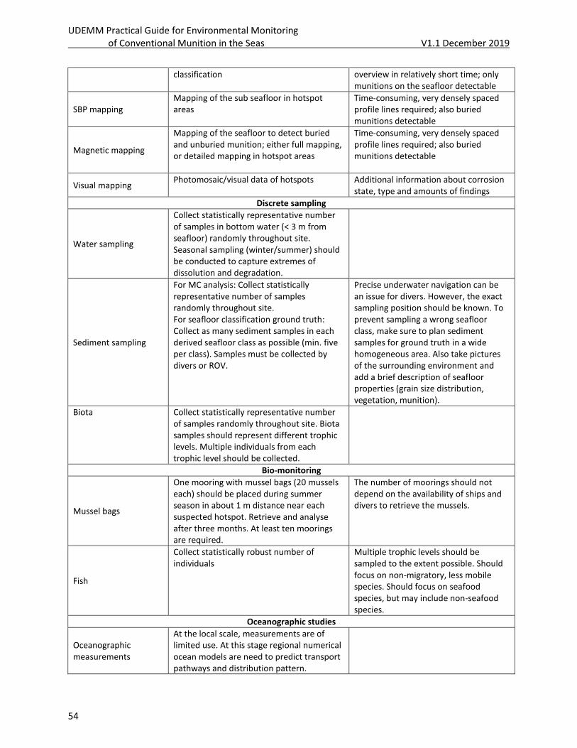
UDEMM Practical Guide for Environmental Monitoring of Conventional Munition in the Seas V1.1 December 2019
54
classification overview in relatively short time; only munitions on the seafloor detectable
SBP mapping Mapping of the sub seafloor in hotspot areas
Time-consuming, very densely spaced profile lines required; also buried munitions detectable
Magnetic mapping
Mapping of the seafloor to detect buried and unburied munition; either full mapping, or detailed mapping in hotspot areas
Time-consuming, very densely spaced profile lines required; also buried munitions detectable
Visual mapping Photomosaic/visual data of hotspots Additional information about corrosion
state, type and amounts of findings
Discrete sampling
Water sampling
Collect statistically representative number of samples in bottom water (< 3 m from seafloor) randomly throughout site. Seasonal sampling (winter/summer) should be conducted to capture extremes of dissolution and degradation.
Sediment sampling
For MC analysis: Collect statistically representative number of samples randomly throughout site. For seafloor classification ground truth: Collect as many sediment samples in each derived seafloor class as possible (min. five per class). Samples must be collected by divers or ROV.
Precise underwater navigation can be an issue for divers. However, the exact sampling position should be known. To prevent sampling a wrong seafloor class, make sure to plan sediment samples for ground truth in a wide homogeneous area. Also take pictures of the surrounding environment and add a brief description of seafloor properties (grain size distribution, vegetation, munition).
Biota Collect statistically representative number of samples randomly throughout site. Biota samples should represent different trophic levels. Multiple individuals from each trophic level should be collected.
Bio-monitoring
Mussel bags
One mooring with mussel bags (20 mussels each) should be placed during summer season in about 1 m distance near each suspected hotspot. Retrieve and analyse after three months. At least ten moorings are required.
The number of moorings should not depend on the availability of ships and divers to retrieve the mussels.
Fish
Collect statistically robust number of individuals
Multiple trophic levels should be sampled to the extent possible. Should focus on non-migratory, less mobile species. Should focus on seafood species, but may include non-seafood species.
Oceanographic studies
Oceanographic measurements
At the local scale, measurements are of limited use. At this stage regional numerical ocean models are need to predict transport pathways and distribution pattern.
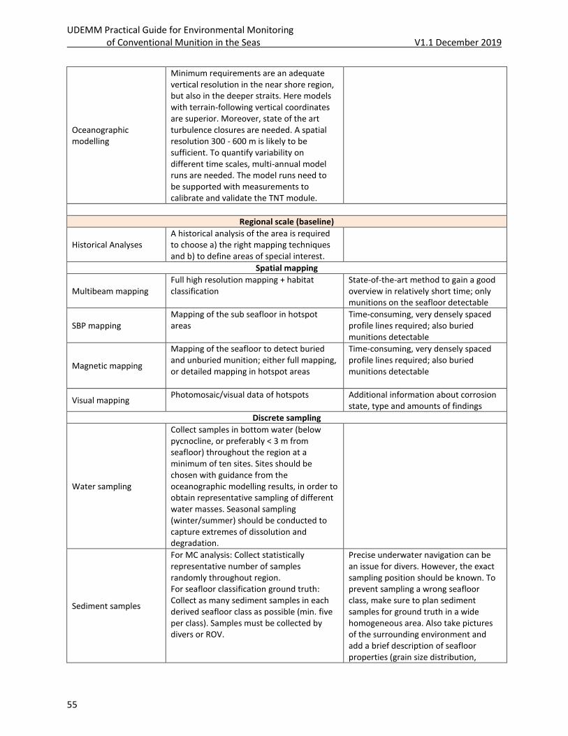
UDEMM Practical Guide for Environmental Monitoring of Conventional Munition in the Seas V1.1 December 2019
55
Oceanographic modelling
Minimum requirements are an adequate vertical resolution in the near shore region, but also in the deeper straits. Here models with terrain-following vertical coordinates are superior. Moreover, state of the art turbulence closures are needed. A spatial resolution 300 - 600 m is likely to be sufficient. To quantify variability on different time scales, multi-annual model runs are needed. The model runs need to be supported with measurements to calibrate and validate the TNT module.
Regional scale (baseline)
Historical Analyses A historical analysis of the area is required to choose a) the right mapping techniques and b) to define areas of special interest.
Spatial mapping
Multibeam mapping Full high resolution mapping + habitat classification
State-of-the-art method to gain a good overview in relatively short time; only munitions on the seafloor detectable
SBP mapping Mapping of the sub seafloor in hotspot areas
Time-consuming, very densely spaced profile lines required; also buried munitions detectable
Magnetic mapping
Mapping of the seafloor to detect buried and unburied munition; either full mapping, or detailed mapping in hotspot areas
Time-consuming, very densely spaced profile lines required; also buried munitions detectable
Visual mapping Photomosaic/visual data of hotspots Additional information about corrosion
state, type and amounts of findings
Discrete sampling
Water sampling
Collect samples in bottom water (below pycnocline, or preferably < 3 m from seafloor) throughout the region at a minimum of ten sites. Sites should be chosen with guidance from the oceanographic modelling results, in order to obtain representative sampling of different water masses. Seasonal sampling (winter/summer) should be conducted to capture extremes of dissolution and degradation.
Sediment samples
For MC analysis: Collect statistically representative number of samples randomly throughout region. For seafloor classification ground truth: Collect as many sediment samples in each derived seafloor class as possible (min. five per class). Samples must be collected by divers or ROV.
Precise underwater navigation can be an issue for divers. However, the exact sampling position should be known. To prevent sampling a wrong seafloor class, make sure to plan sediment samples for ground truth in a wide homogeneous area. Also take pictures of the surrounding environment and add a brief description of seafloor properties (grain size distribution,
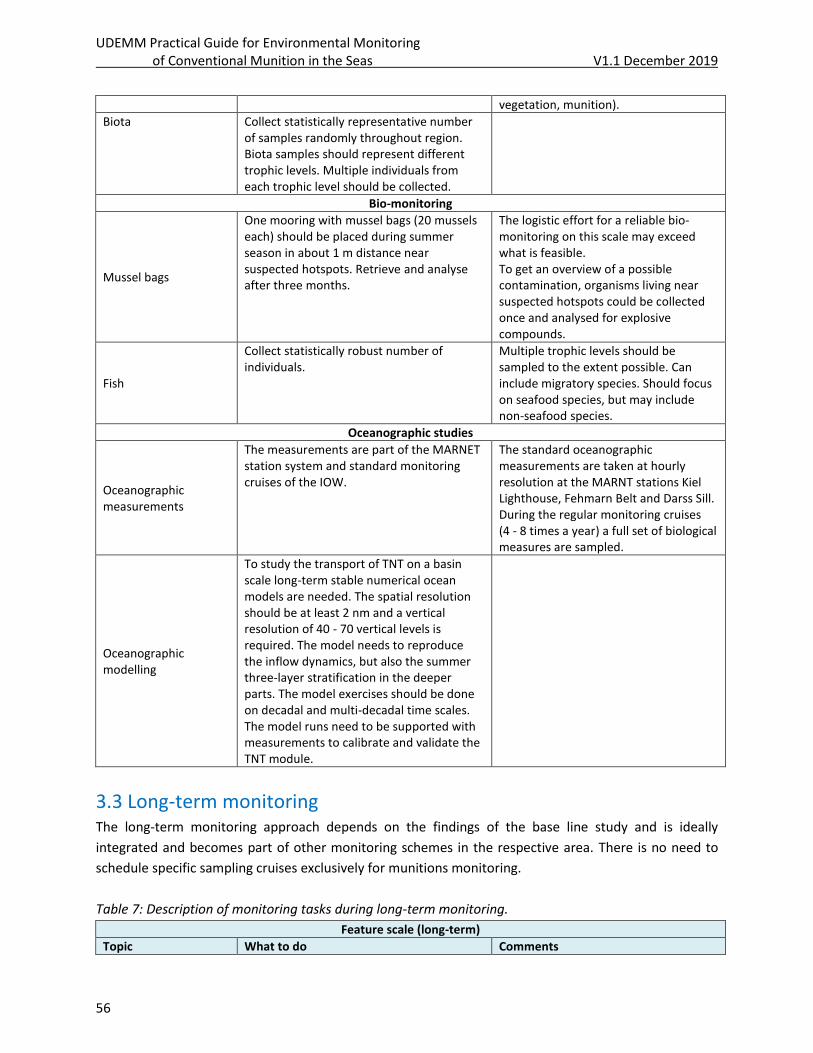
UDEMM Practical Guide for Environmental Monitoring of Conventional Munition in the Seas V1.1 December 2019
56
vegetation, munition).
Biota Collect statistically representative number of samples randomly throughout region. Biota samples should represent different trophic levels. Multiple individuals from each trophic level should be collected.
Bio-monitoring
Mussel bags
One mooring with mussel bags (20 mussels each) should be placed during summer season in about 1 m distance near suspected hotspots. Retrieve and analyse after three months.
The logistic effort for a reliable bio-monitoring on this scale may exceed what is feasible. To get an overview of a possible contamination, organisms living near suspected hotspots could be collected once and analysed for explosive compounds.
Fish
Collect statistically robust number of individuals.
Multiple trophic levels should be sampled to the extent possible. Can include migratory species. Should focus on seafood species, but may include non-seafood species.
Oceanographic studies
Oceanographic measurements
The measurements are part of the MARNET station system and standard monitoring cruises of the IOW.
The standard oceanographic measurements are taken at hourly resolution at the MARNT stations Kiel Lighthouse, Fehmarn Belt and Darss Sill. During the regular monitoring cruises (4 - 8 times a year) a full set of biological measures are sampled.
Oceanographic modelling
To study the transport of TNT on a basin scale long-term stable numerical ocean models are needed. The spatial resolution should be at least 2 nm and a vertical resolution of 40 - 70 vertical levels is required. The model needs to reproduce the inflow dynamics, but also the summer three-layer stratification in the deeper parts. The model exercises should be done on decadal and multi-decadal time scales. The model runs need to be supported with measurements to calibrate and validate the TNT module.
3.3 Long-term monitoring The long-term monitoring approach depends on the findings of the base line study and is ideally
integrated and becomes part of other monitoring schemes in the respective area. There is no need to
schedule specific sampling cruises exclusively for munitions monitoring.
Table 7: Description of monitoring tasks during long-term monitoring.
Feature scale (long-term)
Topic What to do Comments
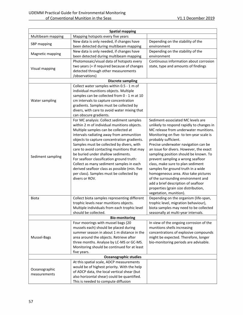
UDEMM Practical Guide for Environmental Monitoring of Conventional Munition in the Seas V1.1 December 2019
57
Spatial mapping
Multibeam mapping Mapping hotspots every five years
SBP mapping New data is only needed, if changes have been detected during multibeam mapping
Depending on the stability of the environment
Magnetic mapping New data is only needed, if changes have been detected during multibeam mapping
Depending on the stability of the environment
Visual mapping
Photomosaic/visual data of hotspots every two years (+ if required because of changes detected through other measurements /observations)
Continuous information about corrosion state, type and amounts of findings
Discrete sampling
Water sampling
Collect water samples within 0.5 - 1 m of individual munitions objects. Multiple samples can be collected from 0 - 1 m at 10 cm intervals to capture concentration gradients. Samples must be collected by divers, with care to avoid water mixing that can obscure gradients.
Sediment sampling
For MC analysis: Collect sediment samples within 2 m of individual munitions objects. Multiple samples can be collected at intervals radiating away from ammunition objects to capture concentration gradients. Samples must be collected by divers, with care to avoid contacting munitions that may be buried under shallow sediments. For seafloor classification ground truth: Collect as many sediment samples in each derived seafloor class as possible (min. five per class). Samples must be collected by divers or ROV.
Sediment-associated MC levels are unlikely to respond rapidly to changes in MC release from underwater munitions. Monitoring on five- to ten-year scale is probably sufficient. Precise underwater navigation can be an issue for divers. However, the exact sampling position should be known. To prevent sampling a wrong seafloor class, make sure to plan sediment samples for ground truth in a wide homogeneous area. Also take pictures of the surrounding environment and add a brief description of seafloor properties (grain size distribution, vegetation, munition).
Biota Collect biota samples representing different trophic levels near munitions objects. Multiple individuals from each trophic level should be collected.
Depending on the organism (life-span, trophic level, migration behaviour), biota samples may need to be collected seasonally at multi-year intervals.
Bio-monitoring
Mussel-Bags
Four moorings with mussel bags (20 mussels each) should be placed during summer season in about 1 m distance in the area around the objects. Retrieve after three months. Analyse by LC-MS or GC-MS. Monitoring should be continued for at least five years.
In view of the ongoing corrosion of the munitions shells increasing concentrations of explosive compounds might be expected. Therefore, longer bio-monitoring periods are advisable.
Oceanographic studies
Oceanographic measurements
At this spatial scale, ADCP measurements would be of highest priority. With the help of ADCP data, the local vertical shear (but also horizontal shear) could be quantified. This is needed to compute diffusion
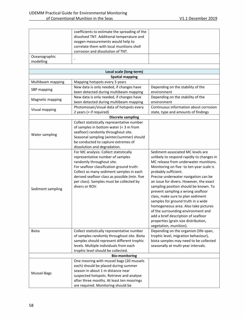
UDEMM Practical Guide for Environmental Monitoring of Conventional Munition in the Seas V1.1 December 2019
58
coefficients to estimate the spreading of the dissolved TNT. Additional temperature and oxygen measurements would help to correlate them with local munitions shell corrosion and dissolution of TNT.
Oceanographic modelling
-
Local scale (long-term)
Spatial mapping
Multibeam mapping Mapping hotspots every 5 years
SBP mapping New data is only needed, if changes have been detected during multibeam mapping
Depending on the stability of the environment
Magnetic mapping New data is only needed, if changes have been detected during multibeam mapping
Depending on the stability of the environment
Visual mapping Photomosaic/visual data of hotspots every 2 years (+ if required)
Continuous information about corrosion state, type and amounts of findings
Discrete sampling
Water sampling
Collect statistically representative number of samples in bottom water (< 3 m from seafloor) randomly throughout site. Seasonal sampling (winter/summer) should be conducted to capture extremes of dissolution and degradation.
Sediment sampling
For MC analysis: Collect statistically representative number of samples randomly throughout site. For seafloor classification ground truth: Collect as many sediment samples in each derived seafloor class as possible (min. five per class). Samples must be collected by divers or ROV.
Sediment-associated MC levels are unlikely to respond rapidly to changes in MC release from underwater munitions. Monitoring on five- to ten-year scale is probably sufficient. Precise underwater navigation can be an issue for divers. However, the exact sampling position should be known. To prevent sampling a wrong seafloor class, make sure to plan sediment samples for ground truth in a wide homogeneous area. Also take pictures of the surrounding environment and add a brief description of seafloor properties (grain size distribution, vegetation, munition).
Biota Collect statistically representative number of samples randomly throughout site. Biota samples should represent different trophic levels. Multiple individuals from each trophic level should be collected.
Depending on the organism (life-span, trophic level, migration behaviour), biota samples may need to be collected seasonally at multi-year intervals.
Bio-monitoring
Mussel-Bags
One mooring with mussel bags (20 mussels each) should be placed during summer season in about 1 m distance near suspected hotspots. Retrieve and analyse after three months. At least ten moorings are required. Monitoring should be
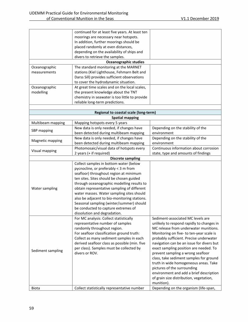
UDEMM Practical Guide for Environmental Monitoring of Conventional Munition in the Seas V1.1 December 2019
59
continued for at least five years. At least ten moorings are necessary near hotspots. In addition, further moorings should be placed randomly at even distances, depending on the availability of ships and divers to retrieve the samples.
Oceanographic studies
Oceanographic measurements
The standard monitoring at the MARNET stations (Kiel Lighthouse, Fehmarn Belt and Darss Sill) provides sufficient observations to cover the hydrodynamic situation.
Oceanographic modelling
At great time scales and on the local scales, the present knowledge about the TNT chemistry in seawater is too little to provide reliable long-term predictions.
Regional to coastal scale (long-term)
Spatial mapping
Multibeam mapping Mapping hotspots every 5 years
SBP mapping New data is only needed, if changes have been detected during multibeam mapping
Depending on the stability of the environment
Magnetic mapping New data is only needed, if changes have been detected during multibeam mapping
Depending on the stability of the environment
Visual mapping Photomosaic/visual data of hotspots every 2 years (+ if required)
Continuous information about corrosion state, type and amounts of findings
Discrete sampling
Water sampling
Collect samples in bottom water (below pycnocline, or preferably < 3 m from seafloor) throughout region at minimum ten sites. Sites should be chosen guided through oceanographic modelling results to obtain representative sampling of different water masses. Water sampling sites should also be adjacent to bio-monitoring stations. Seasonal sampling (winter/summer) should be conducted to capture extremes of dissolution and degradation.
Sediment sampling
For MC analysis: Collect statistically representative number of samples randomly throughout region. For seafloor classification ground truth: Collect as many sediment samples in each derived seafloor class as possible (min. five per class). Samples must be collected by divers or ROV.
Sediment-associated MC levels are unlikely to respond rapidly to changes in MC release from underwater munitions. Monitoring on five- to ten-year scale is probably sufficient. Precise underwater navigation can be an issue for divers but exact sampling position are needed. To prevent sampling a wrong seafloor class, take sediment samples for ground truth in wide homogeneous areas. Take pictures of the surrounding environment and add a brief description of grain size distribution, vegetation, munition).
Biota Collect statistically representative number Depending on the organism (life-span,
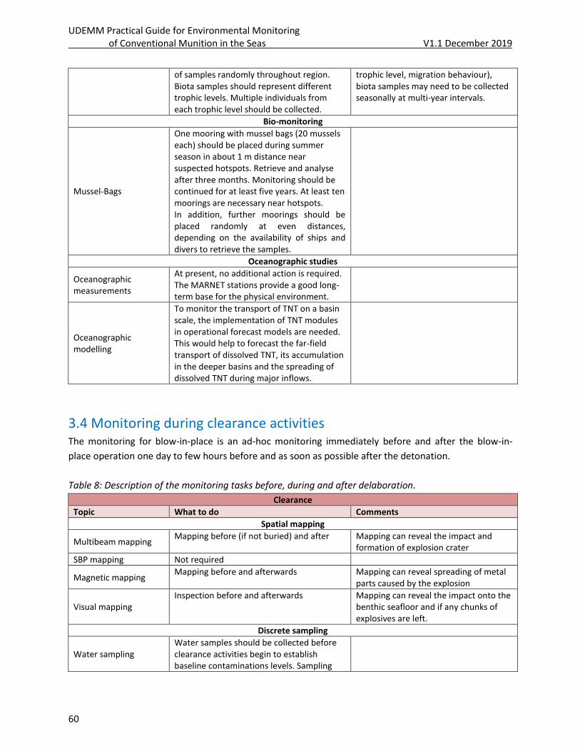
UDEMM Practical Guide for Environmental Monitoring of Conventional Munition in the Seas V1.1 December 2019
60
of samples randomly throughout region. Biota samples should represent different trophic levels. Multiple individuals from each trophic level should be collected.
trophic level, migration behaviour), biota samples may need to be collected seasonally at multi-year intervals.
Bio-monitoring
Mussel-Bags
One mooring with mussel bags (20 mussels each) should be placed during summer season in about 1 m distance near suspected hotspots. Retrieve and analyse after three months. Monitoring should be continued for at least five years. At least ten moorings are necessary near hotspots. In addition, further moorings should be placed randomly at even distances, depending on the availability of ships and divers to retrieve the samples.
Oceanographic studies
Oceanographic measurements
At present, no additional action is required. The MARNET stations provide a good long-term base for the physical environment.
Oceanographic modelling
To monitor the transport of TNT on a basin scale, the implementation of TNT modules in operational forecast models are needed. This would help to forecast the far-field transport of dissolved TNT, its accumulation in the deeper basins and the spreading of dissolved TNT during major inflows.
3.4 Monitoring during clearance activities The monitoring for blow-in-place is an ad-hoc monitoring immediately before and after the blow-in-
place operation one day to few hours before and as soon as possible after the detonation.
Table 8: Description of the monitoring tasks before, during and after delaboration.
Clearance
Topic What to do Comments
Spatial mapping
Multibeam mapping Mapping before (if not buried) and after Mapping can reveal the impact and
formation of explosion crater
SBP mapping Not required
Magnetic mapping Mapping before and afterwards Mapping can reveal spreading of metal
parts caused by the explosion
Visual mapping Inspection before and afterwards Mapping can reveal the impact onto the
benthic seafloor and if any chunks of explosives are left.
Discrete sampling
Water sampling Water samples should be collected before clearance activities begin to establish baseline contaminations levels. Sampling
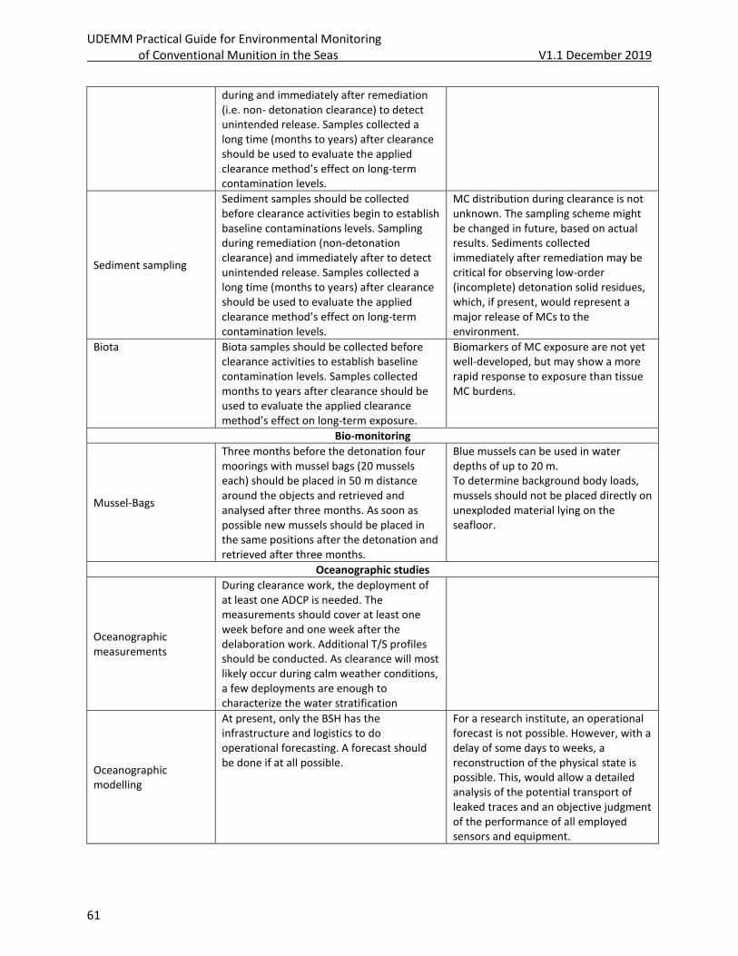
UDEMM Practical Guide for Environmental Monitoring of Conventional Munition in the Seas V1.1 December 2019
61
during and immediately after remediation (i.e. non- detonation clearance) to detect unintended release. Samples collected a long time (months to years) after clearance should be used to evaluate the applied clearance method’s effect on long-term contamination levels.
Sediment sampling
Sediment samples should be collected before clearance activities begin to establish baseline contaminations levels. Sampling during remediation (non-detonation clearance) and immediately after to detect unintended release. Samples collected a long time (months to years) after clearance should be used to evaluate the applied clearance method’s effect on long-term contamination levels.
MC distribution during clearance is not unknown. The sampling scheme might be changed in future, based on actual results. Sediments collected immediately after remediation may be critical for observing low-order (incomplete) detonation solid residues, which, if present, would represent a major release of MCs to the environment.
Biota Biota samples should be collected before clearance activities to establish baseline contamination levels. Samples collected months to years after clearance should be used to evaluate the applied clearance method’s effect on long-term exposure.
Biomarkers of MC exposure are not yet well-developed, but may show a more rapid response to exposure than tissue MC burdens.
Bio-monitoring
Mussel-Bags
Three months before the detonation four moorings with mussel bags (20 mussels each) should be placed in 50 m distance around the objects and retrieved and analysed after three months. As soon as possible new mussels should be placed in the same positions after the detonation and retrieved after three months.
Blue mussels can be used in water depths of up to 20 m. To determine background body loads, mussels should not be placed directly on unexploded material lying on the seafloor.
Oceanographic studies
Oceanographic measurements
During clearance work, the deployment of at least one ADCP is needed. The measurements should cover at least one week before and one week after the delaboration work. Additional T/S profiles should be conducted. As clearance will most likely occur during calm weather conditions, a few deployments are enough to characterize the water stratification
Oceanographic modelling
At present, only the BSH has the infrastructure and logistics to do operational forecasting. A forecast should be done if at all possible.
For a research institute, an operational forecast is not possible. However, with a delay of some days to weeks, a reconstruction of the physical state is possible. This, would allow a detailed analysis of the potential transport of leaked traces and an objective judgment of the performance of all employed sensors and equipment.
UDEMM Practical Guide for Environmental Monitoring of Conventional Munition in the Seas V1.1 December 2019
62
4. Methodologies 4.0 Historical Analysis
Responsible institute: BLANO & MELUND
Historical Analysis (German: Historisch-genetische Rekonstruktion – HGR) consists of several individual
operations and phases. It is completed with a written summary of its results and forms the basis for
subsequent steps in a project. First, the area to be considered is specified. A precise definition is
necessary, in order to focus and to point possible problem areas. After determining the study area an
overview of the history of the entry of munitions is created. This overview contains the assumed age of
expected munitions, combat operations or periods of military trials. On the basis of this list, archive data
for the corresponding area need to be found.
Starting with the local archives, municipal archives, district archives, state archives, federal archives and
military archives, all available data are reviewed according to periods or events and, if necessary,
scanned and saved. Found references to persons and involved military units, ships or authorities are
particularly recorded and also considered and evaluated. If there are indications of possible data
archiving in other archives, such as the Federal Archives of Economic Affairs, Armaments or Industry,
these branches will also be examined.
In the same way, documents in the archives of other countries, especially the Allies of the Second World
War, are examined. The research in these archives is much more difficult because e.g. Britain has a
somewhat more complicated documentation in the existing files. Here, in all likelihood, an investigation
of the involved units and persons must take place in parallel in order to find and evaluate the
appropriate documents.
In addition, data collection and backup is also essential here. All collected documents must be reviewed
and associated. A chronological order is created. Transport units are assigned the daily transport volume
in tons and, if possible, the transported goods. The transport route is reconstructed with the statements
in shipping diaries, harbor dossiers and/or other records and provided with the time and environmental
factors (weather). The type of sinking, as "on-off dumping", en-route-dumping, manual dumping or
dumping by a hopper barge are important facts and show, in connection with the number of crew
members, the quantity of the dumped munitions. After collecting all facts, the result must be verified
through a check of additional historic documents in the manner. If this confirmation agrees with the
determined data, the result can with a high probability be regarded as a real result. These steps are
created individually for each ship, unit or other entity and then combined for the area under review.
Historical datasets can act as a starting point for the definition and specification of monitoring activities.
They indicate historic events (e.g. munitions dumping, war activities) and can be used to specify
sampling strategies in terms of spatial distribution and suspected substances.
Collecting and revising historic data: Military charts, minelaying and minesweeping planes, reports and
other historic data must be collected, digitized and constantly revisited during monitoring activities. The
origin of geodesic dates must be verified and transformed into actual geodesic dates, to ensure
positional accuracy and overlaying of actual and historic spatial information. This process should be
UDEMM Practical Guide for Environmental Monitoring of Conventional Munition in the Seas V1.1 December 2019
63
carried out inside of a specifically designed digital system for visualisation and management of multiple
information sources and measurement data.
Event description: Historic events have to be extracted from the collected data and described including
all relevant information. Multiple independent sources per event should be included for verification and
uncovering of different perspectives. Events should be spatially localized to identify spatial connections
and dimension. Extensive metadata information of specific events (e.g. naval mining, naval combat,
dumping activities) should be recorded including precise information about numbers of objects (e.g.
naval mines), origin of objects and risk originating from objects. In addition, accidents and damages
during transport and routes taken should be recorded. In specific circumstances detailed research has to
be carried out regarding objects and their history e.g. figuring out the composition of MCs. Research and
interpretation have to be carried out including contextual knowledge and data.
Contemporary datasets: Historic information has to be backed/verified by current high-resolution
datasets from bathymetry, side scan sonar, sub-bottom profiler, geomagnetics, photo or video (and if
necessary identification by divers). An assessment of the origin of the objects should be carried out by
EOD specialists and all resulting datasets have to be analysed and managed in a digital system combined
with the acquired historic data.
Evaluation: An ongoing evaluation process has to be established regarding the quality and information
content of the combination of historic and contemporary datasets.
Tools: Management, analysis and visualisation of digitized historic and contemporary datasets should be
generally carried out by functions provided by geographic information systems (GIS). A specifically
designed system for the management of historic datasets in combination with actual measurements is
the Ammunition Cadastre Sea (AmuCad) which in addition includes databases for munitions and
chemicals and incorporates actual research results (DAIMON, North Sea Wrecks).
4.1 Acoustic mapping and monitoring Responsible institute: GEOMAR
The preferably used mapping technique is highly dependent on the dumping ground characteristics,
such as type of ammunition and seafloor properties.
Multibeam echosounder surveys are recommended for unburied objects of a minimum size of 0.5 × 1 m2
in shallow waters of less than 30 m. As the aim of monitoring is to detect changes over time, very high
precision in positioning is required. To reliably quantify object and sediment movements, MBES surveys
shall always be conducted in conjunction with the use of RTK (real time kinematics) services, increasing
GPS accuracies to 5 cm. To perform high resolution multibeam mapping in order to fulfil the IHO special
order (IHO, 2008), a frequency of at least 400 kHz and beam opening angles of maximum 0.5° × 1° are
recommended. Lateral resolutions of min. 20 cm should be achieved. Equidistant mode ensures same
resolution across the entire swath. Swath widths should not exceed 120° and survey speed not more
than 3.5 knots. Although it is time consuming, the surveys shall be conducted with 100 % overlap. For
high data quality it is absolutely necessary to have static offsets, which are well measured and a patch
test performed after each movement of the multibeam relative to the systems components (IMU or GPS
antenna). Sound velocity profiles shall be performed at least twice a survey day. The MBES provides one
tool for three different applications:
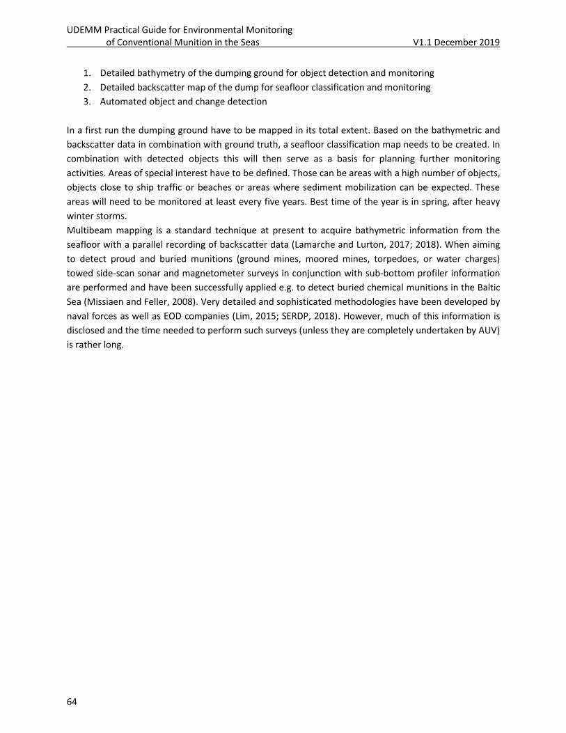
UDEMM Practical Guide for Environmental Monitoring of Conventional Munition in the Seas V1.1 December 2019
64
1. Detailed bathymetry of the dumping ground for object detection and monitoring
2. Detailed backscatter map of the dump for seafloor classification and monitoring
3. Automated object and change detection
In a first run the dumping ground have to be mapped in its total extent. Based on the bathymetric and
backscatter data in combination with ground truth, a seafloor classification map needs to be created. In
combination with detected objects this will then serve as a basis for planning further monitoring
activities. Areas of special interest have to be defined. Those can be areas with a high number of objects,
objects close to ship traffic or beaches or areas where sediment mobilization can be expected. These
areas will need to be monitored at least every five years. Best time of the year is in spring, after heavy
winter storms.
Multibeam mapping is a standard technique at present to acquire bathymetric information from the
seafloor with a parallel recording of backscatter data (Lamarche and Lurton, 2017; 2018). When aiming
to detect proud and buried munitions (ground mines, moored mines, torpedoes, or water charges)
towed side-scan sonar and magnetometer surveys in conjunction with sub-bottom profiler information
are performed and have been successfully applied e.g. to detect buried chemical munitions in the Baltic
Sea (Missiaen and Feller, 2008). Very detailed and sophisticated methodologies have been developed by
naval forces as well as EOD companies (Lim, 2015; SERDP, 2018). However, much of this information is
disclosed and the time needed to perform such surveys (unless they are completely undertaken by AUV)
is rather long.
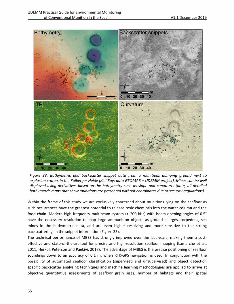
UDEMM Practical Guide for Environmental Monitoring of Conventional Munition in the Seas V1.1 December 2019
65
Figure 33: Bathymetric and backscatter snippet data from a munitions dumping ground next to explosion craters in the Kolberger Heide (Kiel Bay; data GEOMAR – UDEMM project). Mines can be well displayed using derivatives based on the bathymetry such as slope and curvature. (note, all detailed bathymetric maps that show munitions are presented without coordinates due to security regulations).
Within the frame of this study we are exclusively concerned about munitions lying on the seafloor as
such occurrences have the greatest potential to release toxic chemicals into the water column and the
food chain. Modern high frequency multibeam system (> 200 kHz) with beam opening angles of 0.5°
have the necessary resolution to map large ammunition objects as ground charges, torpedoes, sea
mines in the bathymetric data, and are even higher resolving and more sensitive to the strong
backscattering, in the snippet information (Figure 33).
The technical performance of MBES has strongly improved over the last years, making them a cost-
effective and state-of-the-art tool for precise and high-resolution seafloor mapping (Lamarche et al.,
2011; Herkül, Peterson and Paekivi, 2017). The advantage of MBES is the precise positioning of seafloor
soundings down to an accuracy of 0.1 m, when RTK-GPS navigation is used. In conjunction with the
possibility of automated seafloor classification (supervised and unsupervised) and object detection
specific backscatter analysing techniques and machine learning methodologies are applied to arrive at
objective quantitative assessments of seafloor grain sizes, number of habitats and their spatial

UDEMM Practical Guide for Environmental Monitoring of Conventional Munition in the Seas V1.1 December 2019
66
distribution (Alevizos et al., 2015; 2018). In addition, they help to detect munitions either via supervised
classification based on a classification dictionary (Figure 34) or machine learning algorithms as Random
Forest, Artificial Neural Networks, or Supported Vector Machines. Such calculations can be done in GIS
environments (e.g. ArcGIS, SAGA) or other software packages like MatLab.
Figure 34: Results from a hydroacoustic survey in the area of Kolberger Heide. Top: Bathymetric map of the central Kolberger Heide with all identified mines marked with triangles; below: Seafloor Classification map based on the multibeam backscatter distribution and ground truth data (video and sediment samples).
Bathymetric derivatives such as slope (Figure 33), bathymetric positioning index (BPI), curvature,
rugosity, or concavity (Figure 33), have been proven to be correlated to different kinds of habitats
(McGonigle et al., 2009). In addition, backscatter data and their statistics also show close correlation and
UDEMM Practical Guide for Environmental Monitoring of Conventional Munition in the Seas V1.1 December 2019
67
are jointly used for a statistically valid seafloor classification with respect to sediment grain size (Alevizos
et al., 2015; 2017).
During the UDEMM project, several multibeam surveys have been conducted in the area of the
munitions dumping ground Kolberger Heide and based on the generated multibeam map
sampling/monitoring locations were planned. Several sites of interest were identified for further
investigation with geochemical and bio-monitoring methods. In combination with ground truth data a
seafloor classification map was generated, that provides information about the seafloor coverage by
algae. In the Kolberger Heide, large amounts of conventional munitions in form of moored mines (1.5 m
diameter), ground mines (2.5 m length) and water bombs (1 × 0.5 m) can be found.
References:
Alevizos, E. et al. (2015) ‘Acoustic discrimination of relatively homogeneous fine sediments using Bayesian
classification on MBES data’, Marine Geology, 370, pp. 31–42. doi: 10.1016/j.margeo.2015.10.007.
Alevizos, E. et al. (2018) ‘Multi-angle backscatter classification and sub-bottom profiling for improved seafloor
characterization’, Marine Geophysical Research. Springer Netherlands, 39(1–2), pp. 289–306. doi:
10.1007/s11001-017-9325-4.
Brown, C. J. et al. (2011) ‘Benthic habitat mapping: A review of progress towards improved understanding of the
spatial ecology of the seafloor using acoustic techniques’, Estuarine, Coastal and Shelf Science. Elsevier Ltd,
92(3), pp. 502–520. doi: 10.1016/j.ecss.2011.02.007.
Calvert, J. et al. (2015) ‘An evaluation of supervised and unsupervised classification techniques for marine benthic
habitat mapping using multibeam echosounder data’, ICES Journal of Marine Science. doi:
10.1093/icesjms/fsu223.
Herkül, K., Peterson, A. and Paekivi, S. (2017) ‘Applying multibeam sonar and mathematical modelling for mapping
seabed substrate and biota of offshore shallows’, Estuarine, Coastal and Shelf Science. Elsevier Ltd, 192, pp.
57–71. doi: 10.1016/j.ecss.2017.04.026.
IHO (2008) IHO Standards. 6th edn; https://www.iho.int/iho_pubs/draft_pubs/S-44_Edition_6_draft_1_7_1.pdf.
Lamarche, G. et al. (2011) ‘Quantitative characterisation of seafloor substrate and bedforms using advanced
processing of multibeam backscatter-Application to Cook Strait, New Zealand’, Continental Shelf Research,
31(2 SUPPL.), pp. 93–109. doi: 10.1016/j.csr.2010.06.001.
Lamarche, G. and Lurton, X. (2017) ‘Recommendations for improved and coherent acquisition and processing of
backscatter data from seafloor-mapping sonars’, Marine Geophysical Research. doi: 10.1007/s11001-017-
9315-6.
Lamarche, G. and Lurton, X. (2018) ‘Recommendations for improved and coherent acquisition and processing of
backscatter data from seafloor-mapping sonars’, Marine Geophysical Research. Springer Netherlands, 39(1–
2), pp. 5–22. doi: 10.1007/s11001-017-9315-6.
Lim, R. (2015) ‘Data and Processing Tools for Sonar Classification of Underwater UXO’, Technical report, SERDP
Project, (August), pp. 1–2.
McGonigle, C. et al. (2009) ‘Evaluation of image-based multibeam sonar backscatter classification for benthic
habitat discrimination and mapping at Stanton Banks, UK’, Estuarine, Coastal and Shelf Science. Elsevier Ltd,
81(3), pp. 423–437. doi: 10.1016/j.ecss.2008.11.017.
Missiaen, T. and Feller, P. (2008) ‘Very-high-resolution seismic and magnetic investigations of a chemical munition
dumpsite in the Baltic Sea’, Journal of Applied Geophysics, 65(3–4), pp. 142–154. doi:
10.1016/j.jappgeo.2008.07.001.
SERDP (2018) FINAL REPORT SERDP Workshop on Acoustic Detection and Classification of Munitions in the
Underwater Environment April 2018.
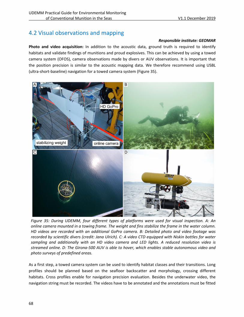
UDEMM Practical Guide for Environmental Monitoring of Conventional Munition in the Seas V1.1 December 2019
68
4.2 Visual observations and mapping Responsible institute: GEOMAR
Photo and video acquisition: In addition to the acoustic data, ground truth is required to identify
habitats and validate findings of munitions and proud explosives. This can be achieved by using a towed
camera system (OFOS), camera observations made by divers or AUV observations. It is important that
the position precision is similar to the acoustic mapping data. We therefore recommend using USBL
(ultra-short-baseline) navigation for a towed camera system (Figure 35).
Figure 35: During UDEMM, four different types of platforms were used for visual inspection. A: An online camera mounted in a towing frame. The weight and fins stabilize the frame in the water column. HD videos are recorded with an additional GoPro camera. B: Detailed photo and video footage was recorded by scientific divers (credit: Jana Ulrich). C: A video CTD equipped with Niskin bottles for water sampling and additionally with an HD video camera and LED lights. A reduced resolution video is streamed online. D: The Girona-500 AUV is able to hover, which enables stable autonomous video and photo surveys of predefined areas.
As a first step, a towed camera system can be used to identify habitat classes and their transitions. Long
profiles should be planned based on the seafloor backscatter and morphology, crossing different
habitats. Cross profiles enable for navigation precision evaluation. Besides the underwater video, the
navigation string must be recorded. The videos have to be annotated and the annotations must be fitted
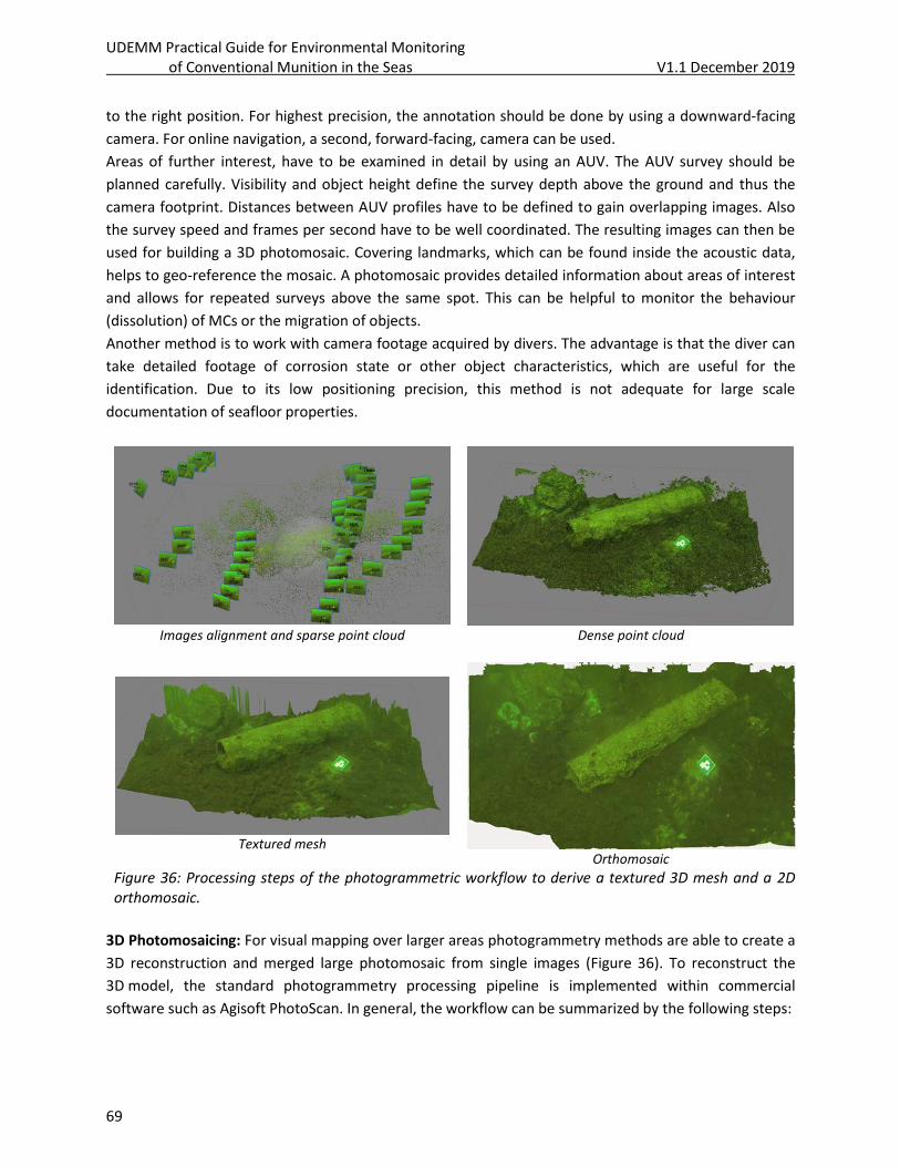
UDEMM Practical Guide for Environmental Monitoring of Conventional Munition in the Seas V1.1 December 2019
69
to the right position. For highest precision, the annotation should be done by using a downward-facing
camera. For online navigation, a second, forward-facing, camera can be used.
Areas of further interest, have to be examined in detail by using an AUV. The AUV survey should be
planned carefully. Visibility and object height define the survey depth above the ground and thus the
camera footprint. Distances between AUV profiles have to be defined to gain overlapping images. Also
the survey speed and frames per second have to be well coordinated. The resulting images can then be
used for building a 3D photomosaic. Covering landmarks, which can be found inside the acoustic data,
helps to geo-reference the mosaic. A photomosaic provides detailed information about areas of interest
and allows for repeated surveys above the same spot. This can be helpful to monitor the behaviour
(dissolution) of MCs or the migration of objects.
Another method is to work with camera footage acquired by divers. The advantage is that the diver can
take detailed footage of corrosion state or other object characteristics, which are useful for the
identification. Due to its low positioning precision, this method is not adequate for large scale
documentation of seafloor properties.
Images alignment and sparse point cloud
Dense point cloud
Textured mesh
Orthomosaic
Figure 36: Processing steps of the photogrammetric workflow to derive a textured 3D mesh and a 2D orthomosaic.
3D Photomosaicing: For visual mapping over larger areas photogrammetry methods are able to create a
3D reconstruction and merged large photomosaic from single images (Figure 36). To reconstruct the
3D model, the standard photogrammetry processing pipeline is implemented within commercial
software such as Agisoft PhotoScan. In general, the workflow can be summarized by the following steps:
UDEMM Practical Guide for Environmental Monitoring of Conventional Munition in the Seas V1.1 December 2019
70
1. Load the images and align the images. This step extracts feature (key) points from images and
tries to match the feature points between images. The matching results will then be used to
estimate the exact camera position and orientation of each image and generate the sparse point
cloud from the feature points.
2. Build the dense point cloud. The subsequent dense matching algorithm tries to find the
corresponding matches for each pixel within the following image in order to generate a dense
point cloud. Each dense matching result is stored in a depth map form. Afterwards, all depth
maps are fused into a unified dense point cloud model.
3. Georeference the point cloud. Due to the lack of any reference information (absolute position),
the dense point cloud is still unscaled and not georeferenced. There are two common ways to
georeference the model, one is to record position date (e.g. GPS, USBL) with the images when
they were captured and provide them while loading the images. Another way is give at least
three known coordinates within the dense point cloud when it is generated.
4. Build the mesh model from the dense point cloud. Software specific to PhotoScan, one chooses
surface type as “Height field (2.5D)” to build the polygonal (triangle) mesh from the dense point
cloud.
5. Build model texture and generate the orthomosaic. PhotoScan projects all the meshes into a
virtual ortho-view plane and each projected mesh is textured by the patch from the original
images. This results in the final photomosaic.
One drawback when dealing with underwater images is that all photogrammetric software packages
that are currently on the market focus on in non-aquatic applications. Due to several water effects, in
both geometry and radiometry aspects, the refracted geometry and attenuated colour information in
underwater images make the 3D reconstruction more difficult than the application in air. Thus,
additional efforts are needed to make the current software applicable for underwater uses, especially
for large scale AUV mapping purposes. GEOMAR thus developed an iterative refinement approach to
link with PhotoScan for underwater reconstruction tasks. This approach utilizes the initial reconstruction
results from PhotoScan to correct the water effects in the images, and then feeds these corrected
images as input to the next reconstruction iteration until the reconstruction results between two
iterations converged. More details about this iterative approach have been recently published by Song
et al. (2019) . A large scale reconstruction of underwater munitions boxes (reconstructed from 1,059
images) taken by an AUV in the Bay of Lübeck, is shown in Figure 37 and Figure 38.

UDEMM Practical Guide for Environmental Monitoring of Conventional Munition in the Seas V1.1 December 2019
71
Figure 37: On the left side: A photomosaic of munitions boxes was created based on photo profiles run by the GIRONA-500 AUV from GEOMAR. Right side: 3D model calculated from the photomosaic.
Top and side view of original 3D mesh output from PhotoScan
Top and side view of refined 3D mesh
Figure 38: Photogrammetric reconstruction of images acquired in the Bay of Lübeck. The upper two images show the original PhotoScan results. The lower two images show the iteration approach developed by GEOMAR, now with a flat and correct seafloor.
UDEMM Practical Guide for Environmental Monitoring of Conventional Munition in the Seas V1.1 December 2019
72
Reference:
Song, Y., Köser, K., Kwasnitschka, T., and Koch, R. (2019) ITERATIVE REFINEMENT FOR UNDERWATER 3D
RECONSTRUCTION: APPLICATION TO DISPOSED UNDERWATER MUNITIONS IN THE BALTIC SEA, Int. Arch.
Photogramm. Remote Sens. Spatial Inf. Sci., XLII-2/W10, 181-187, https://doi.org/10.5194/isprs-archives-
XLII-2-W10-181-2019.
4.3 Field sampling of sediment and biota Responsible institute: GEOMAR
Sediment and biota can be collected using a Van Veen-type surface grab or coring apparatus in areas
where there is no risk of encountering submerged munitions. Where there is a risk of hitting
submerged munition, samples must be collected by properly trained divers only.
Sediment samples are performed for grain size analyses and other sediment properties. The sediment
grain size allows to assess the acoustic properties of the sediment . In combination with the underwater
footage it is the base for a habitat map. The positioning precision of the sample has to be as close as
possible to the acoustic positioning precision. Otherwise it is impossible to correlate it with the right
habitat. For grain size analysis the sample size is dependent on the grain size. The coarser a sample, the
larger it needs to be, to give representative results. The sampling spot should additionally be
documented via photo and a brief description. The sample does not necessarily have to be cooled. In the
lab it has to be sieved or analysed by a laser particle analyser according to the sediment classes
proposed by Blott and Pye (2012).
Sediment sampling for later TNT analysis is done as for regular sediment samples, but samples must be
stored frozen at -18 °C until further processing. Samples for total metal content measurements should
be stored frozen as well. If sediment mineral phases are to be determined (e.g. authigenic oxide or
sulphide minerals), samples cannot be stored long term even if frozen, and must be processed
immediately.
Biota (e.g. algae clumps, sea stars, mussels) can be collected manually by divers. If aggregations of algae
or mussels are transferred immediately to fine mesh or plastic bags, associated organisms such as
worms and crustaceans can also be obtained. Sediment infauna are collected from surface grabs. A
0.5 mm sieve can be used to separate organisms from the sediment matrix. Like sediments, biota
samples should be stored frozen.
4.4 Habitat mapping Responsible institute: GEOMAR
To describe the seafloor properties of the monitored dumping ground, the creation of a habitat map is
needed. This will give information about sediment composition and floral distribution within this area.
Both is needed, to evaluate the best areas for deploying monitoring moorings and to identify areas,
which need special observation. Depending on the seafloor, different methods might be chosen for
mine detection.
As input raster set a combination of seafloor backscatter and morphological derivatives have to be
created. Which data is used, depends on the seafloor of the area. If the variability is mostly defined by
changes within sediments, the backscatter is more important than morphological derivatives. (Brown et
UDEMM Practical Guide for Environmental Monitoring of Conventional Munition in the Seas V1.1 December 2019
73
al., 2011) On the other hand, if topographic features dominate, derivatives, which best describe these,
have to be developed. This can be done by the use of GIS programs like e.g. SAGA GIS, QGIS or ArcGIS.
All input rasters have to have the same spatial extent and cell size.
There are different seafloor classification methods. One example is an unsupervised classification, using
the ArcGIS ‘ISO Cluster and Maximum Likelihood Classification’ tool, which classifies the data based on
the raster values and creates classes of similar value distributions (Calvert et al., 2015). The resulting
classes have to be compared to the ground truth data (video, images, sediment samples, seafloor
description) in order to identify habitats. Ground truthing should be planned based on the classification
map, in order to sample each class multiple times.
Another method is to perform a supervised classification. For this, for known habitats (validated by the
ground truth), the individual raster values will be analysed and assigned to a specific habitat. The
habitats can then be spatially extrapolated (Hasan, Ierodiaconou and Monk, 2012). This method
guarantees that each ground truth identified habitat will be mapped. On the other hand, a high number
of ground truth samples is required, in order not to miss a distinct habitat.
With the unsupervised classification, ground truthing can be planned specifically, which saves survey
time.
Which method is preferably used depends on the heterogeneity of the survey area. The more small
scale variability can be found, the more ground truth data is needed. In order to make sure not to miss a
certain habitat, unsupervised classification should be the first choice in that case.
References:
Brown, C. J. et al. (2011) ‘Benthic habitat mapping: A review of progress towards improved understanding of the
spatial ecology of the seafloor using acoustic techniques’, Estuarine, Coastal and Shelf Science. Elsevier Ltd,
92(3), pp. 502–520. doi: 10.1016/j.ecss.2011.02.007.
Calvert, J. et al. (2015) ‘An evaluation of supervised and unsupervised classification techniques for marine benthic
habitat mapping using multibeam echosounder data’, ICES Journal of Marine Science. doi:
10.1093/icesjms/fsu223.
Hasan, R. C., Ierodiaconou, D. and Monk, J. (2012) ‘Evaluation of four supervised learning methods for benthic
habitat mapping using backscatter from multi-beam sonar’, Remote Sensing, 4(11), pp. 3427–3443. doi:
10.3390/rs4113427.
4.5 Oceanographic monitoring Responsible institute: IOW
To characterize the physical/hydrodynamic environment, in situ measurements of currents, bottom
salinity and bottom temperature at the munitions dumping ground are needed. For this purpose an
ADCP, for shallow waters up to 12 m depth a 1,200kHz ADCP, or otherwise a 600kHz ADCP for deeper
waters, and a SeaCat should be used. The positioning of the instruments should be at the deepest point
of the munitions dumping ground to provide the broadest possible overview of the water column for
current measurements. To ensure exactly vertical measurements, the ADCP should be mounted in a
gimbaled frame, with the SeaCat besides it, such that the SeaCat does not interfere with the beams of
the ADCP. To avoid munitions contact, divers should deploy this frame. The SeaCat and the ADCP should
provide one measurement every 15 min, whereby the ADCP measurement should be a mean value of a
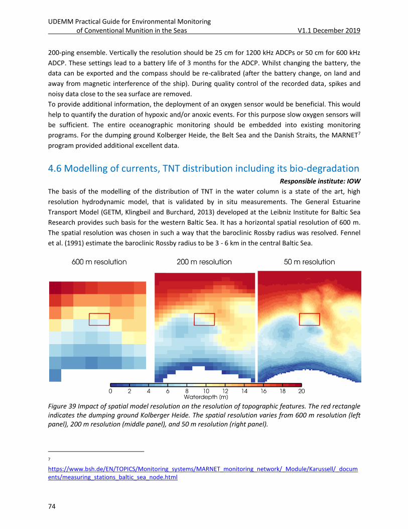
UDEMM Practical Guide for Environmental Monitoring of Conventional Munition in the Seas V1.1 December 2019
74
200-ping ensemble. Vertically the resolution should be 25 cm for 1200 kHz ADCPs or 50 cm for 600 kHz
ADCP. These settings lead to a battery life of 3 months for the ADCP. Whilst changing the battery, the
data can be exported and the compass should be re-calibrated (after the battery change, on land and
away from magnetic interference of the ship). During quality control of the recorded data, spikes and
noisy data close to the sea surface are removed.
To provide additional information, the deployment of an oxygen sensor would be beneficial. This would
help to quantify the duration of hypoxic and/or anoxic events. For this purpose slow oxygen sensors will
be sufficient. The entire oceanographic monitoring should be embedded into existing monitoring
programs. For the dumping ground Kolberger Heide, the Belt Sea and the Danish Straits, the MARNET7
program provided additional excellent data.
4.6 Modelling of currents, TNT distribution including its bio-degradation Responsible institute: IOW
The basis of the modelling of the distribution of TNT in the water column is a state of the art, high
resolution hydrodynamic model, that is validated by in situ measurements. The General Estuarine
Transport Model (GETM, Klingbeil and Burchard, 2013) developed at the Leibniz Institute for Baltic Sea
Research provides such basis for the western Baltic Sea. It has a horizontal spatial resolution of 600 m.
The spatial resolution was chosen in such a way that the baroclinic Rossby radius was resolved. Fennel
et al. (1991) estimate the baroclinic Rossby radius to be 3 - 6 km in the central Baltic Sea.
Figure 39 Impact of spatial model resolution on the resolution of topographic features. The red rectangle indicates the dumping ground Kolberger Heide. The spatial resolution varies from 600 m resolution (left panel), 200 m resolution (middle panel), and 50 m resolution (right panel).
7 https://www.bsh.de/EN/TOPICS/Monitoring_systems/MARNET_monitoring_network/_Module/Karussell/_documents/measuring_stations_baltic_sea_node.html
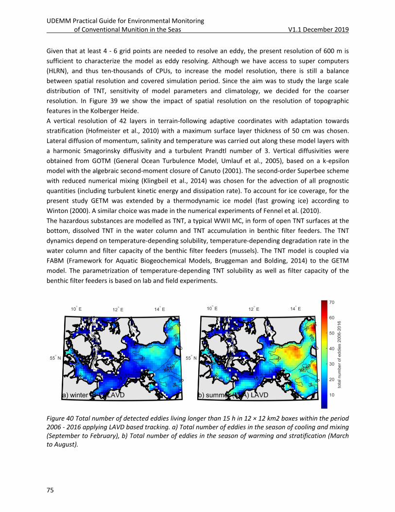
UDEMM Practical Guide for Environmental Monitoring of Conventional Munition in the Seas V1.1 December 2019
75
Given that at least 4 - 6 grid points are needed to resolve an eddy, the present resolution of 600 m is
sufficient to characterize the model as eddy resolving. Although we have access to super computers
(HLRN), and thus ten-thousands of CPUs, to increase the model resolution, there is still a balance
between spatial resolution and covered simulation period. Since the aim was to study the large scale
distribution of TNT, sensitivity of model parameters and climatology, we decided for the coarser
resolution. In Figure 39 we show the impact of spatial resolution on the resolution of topographic
features in the Kolberger Heide.
A vertical resolution of 42 layers in terrain-following adaptive coordinates with adaptation towards
stratification (Hofmeister et al., 2010) with a maximum surface layer thickness of 50 cm was chosen.
Lateral diffusion of momentum, salinity and temperature was carried out along these model layers with
a harmonic Smagorinsky diffusivity and a turbulent Prandtl number of 3. Vertical diffusivities were
obtained from GOTM (General Ocean Turbulence Model, Umlauf et al., 2005), based on a k-epsilon
model with the algebraic second-moment closure of Canuto (2001). The second-order Superbee scheme
with reduced numerical mixing (Klingbeil et al., 2014) was chosen for the advection of all prognostic
quantities (including turbulent kinetic energy and dissipation rate). To account for ice coverage, for the
present study GETM was extended by a thermodynamic ice model (fast growing ice) according to
Winton (2000). A similar choice was made in the numerical experiments of Fennel et al. (2010).
The hazardous substances are modelled as TNT, a typical WWII MC, in form of open TNT surfaces at the
bottom, dissolved TNT in the water column and TNT accumulation in benthic filter feeders. The TNT
dynamics depend on temperature-depending solubility, temperature-depending degradation rate in the
water column and filter capacity of the benthic filter feeders (mussels). The TNT model is coupled via
FABM (Framework for Aquatic Biogeochemical Models, Bruggeman and Bolding, 2014) to the GETM
model. The parametrization of temperature-depending TNT solubility as well as filter capacity of the
benthic filter feeders is based on lab and field experiments.
Figure 40 Total number of detected eddies living longer than 15 h in 12 × 12 km2 boxes within the period 2006 - 2016 applying LAVD based tracking. a) Total number of eddies in the season of cooling and mixing (September to February), b) Total number of eddies in the season of warming and stratification (March to August).
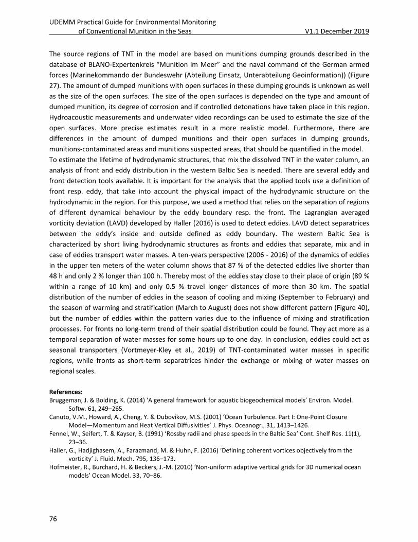
UDEMM Practical Guide for Environmental Monitoring of Conventional Munition in the Seas V1.1 December 2019
76
The source regions of TNT in the model are based on munitions dumping grounds described in the
database of BLANO-Expertenkreis “Munition im Meer” and the naval command of the German armed
forces (Marinekommando der Bundeswehr (Abteilung Einsatz, Unterabteilung Geoinformation)) (Figure
27). The amount of dumped munitions with open surfaces in these dumping grounds is unknown as well
as the size of the open surfaces. The size of the open surfaces is depended on the type and amount of
dumped munition, its degree of corrosion and if controlled detonations have taken place in this region.
Hydroacoustic measurements and underwater video recordings can be used to estimate the size of the
open surfaces. More precise estimates result in a more realistic model. Furthermore, there are
differences in the amount of dumped munitions and their open surfaces in dumping grounds,
munitions-contaminated areas and munitions suspected areas, that should be quantified in the model.
To estimate the lifetime of hydrodynamic structures, that mix the dissolved TNT in the water column, an
analysis of front and eddy distribution in the western Baltic Sea is needed. There are several eddy and
front detection tools available. It is important for the analysis that the applied tools use a definition of
front resp. eddy, that take into account the physical impact of the hydrodynamic structure on the
hydrodynamic in the region. For this purpose, we used a method that relies on the separation of regions
of different dynamical behaviour by the eddy boundary resp. the front. The Lagrangian averaged
vorticity deviation (LAVD) developed by Haller (2016) is used to detect eddies. LAVD detect separatrices
between the eddy’s inside and outside defined as eddy boundary. The western Baltic Sea is
characterized by short living hydrodynamic structures as fronts and eddies that separate, mix and in
case of eddies transport water masses. A ten-years perspective (2006 - 2016) of the dynamics of eddies
in the upper ten meters of the water column shows that 87 % of the detected eddies live shorter than
48 h and only 2 % longer than 100 h. Thereby most of the eddies stay close to their place of origin (89 %
within a range of 10 km) and only 0.5 % travel longer distances of more than 30 km. The spatial
distribution of the number of eddies in the season of cooling and mixing (September to February) and
the season of warming and stratification (March to August) does not show different pattern (Figure 40),
but the number of eddies within the pattern varies due to the influence of mixing and stratification
processes. For fronts no long-term trend of their spatial distribution could be found. They act more as a
temporal separation of water masses for some hours up to one day. In conclusion, eddies could act as
seasonal transporters (Vortmeyer-Kley et al., 2019) of TNT-contaminated water masses in specific
regions, while fronts as short-term separatrices hinder the exchange or mixing of water masses on
regional scales.
References: Bruggeman, J. & Bolding, K. (2014) ‘A general framework for aquatic biogeochemical models’ Environ. Model.
Softw. 61, 249–265. Canuto, V.M., Howard, A., Cheng, Y. & Dubovikov, M.S. (2001) ‘Ocean Turbulence. Part I: One-Point Closure
Model—Momentum and Heat Vertical Diffusivities’ J. Phys. Oceanogr., 31, 1413–1426. Fennel, W., Seifert, T. & Kayser, B. (1991) ‘Rossby radii and phase speeds in the Baltic Sea’ Cont. Shelf Res. 11(1),
23–36. Haller, G., Hadjighasem, A., Farazmand, M. & Huhn, F. (2016) ‘Defining coherent vortices objectively from the
vorticity’ J. Fluid. Mech. 795, 136–173. Hofmeister, R., Burchard, H. & Beckers, J.-M. (2010) ‘Non-uniform adaptive vertical grids for 3D numerical ocean
models’ Ocean Model. 33, 70–86.
UDEMM Practical Guide for Environmental Monitoring of Conventional Munition in the Seas V1.1 December 2019
77
Klingbeil, K. & Burchard, H. (2013) ‘Implementation of a direct nonhydrostatic pressure gradient discretisation into a layered ocean model’ Ocean Model. 65, 64-77.
Klingbeil, K., Mohammadi-Aragh, M., Gräwe, U. & Burchard, H. (2014) ‘Quantification of spurious dissipation and mixing – Discrete variance decay in a Finite-Volume framework’. Ocean Model. 81, 49-64.
Umlauf, L. & Burchard, H. (2005) ‘Second-order turbulence closure models for geophysical boundary layers. A review of recent work’ Cont. Shelf Res. 25 (7–8), 795-827.
Vortmeyer-Kley, R., Lünsmann, B., Berthold, M., Gräwe, U. & Feudel, U. Eddies (2019) ‘Fluid Dynamical Niches or Transporters? – A Case Study in the Western Baltic Sea’ Front. Mar. Sci. 6.
4.7 Water sampling Responsible institute: GEOMAR
All samples should be protected from heat and light, as the target MCs are sensitive to both and may
undergo transformation or degradation. Water samples are collected using either a pump system or
Niskin bottles. Munitions act as point sources of MCs, which are rapidly diluted upon release. As a result,
it is preferable, to collect water samples with Niskin bottles, to avoid ship drifting out of the munitions
plume during pumping. Water samples may also be collected by divers in closer proximity to the
munitions. More than 99 % of MCs in the water column appear to be in the dissolved phase (< 0.2 µm),
so sample filtration does not appear necessary. However, degradation experiments indicate that sterile
filtered samples are stable at 8 °C for up to 10 d, while unfiltered samples must be extracted and the
MCs frozen immediately after collection. Suspended particles are collected with 0.2 µm Sterivex filters
(filtrate can be reserved for dissolved MC analysis). Solvent-resistant membrane material (e.g. PTFE,
PVDF) should be used, to allow MC extraction directly within the filter capsule.
TNT and other MCs can be adsorbed by plastic sampling materials, which indeed forms the basis for
passive sampling of MCs in natural waters (e.g., Warren et al., 2019; Lotufo et al., 2019). In tests with
plastic sampling materials used in UDEMM (amber HDPE bottles, PP centrifuge tubes) negligible
adsorption of target within the short holding time was observed (Beck et al., 2019). Nonetheless, care
should be taken, to ensure that samples for MC analysis are not stored in plastic containers for extended
periods of time.
Figure 41: Recovery of stable isotope-labelled TNT and DNB. Error bars represent standard deviation of the mean of triplicate incubations (from Beck et al., 2019).
Previous results showed that MC distributions in the water column were highly variable in both space
and time, and that high resolution sampling is required to adequately monitor the regional magnitude
and extent of contaminant plumes from underwater munitions dumping grounds. As a result, the
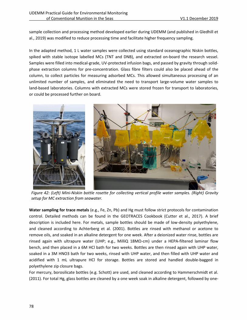
UDEMM Practical Guide for Environmental Monitoring of Conventional Munition in the Seas V1.1 December 2019
78
sample collection and processing method developed earlier during UDEMM (and published in Gledhill et
al., 2019) was modified to reduce processing time and facilitate higher frequency sampling.
In the adapted method, 1 L water samples were collected using standard oceanographic Niskin bottles,
spiked with stable isotope labelled MCs (TNT and DNB), and extracted on-board the research vessel.
Samples were filled into medical-grade, UV-protected infusion bags, and passed by gravity through solid-
phase extraction columns for pre-concentration. Glass fibre filters could also be placed ahead of the
column, to collect particles for measuring adsorbed MCs. This allowed simultaneous processing of an
unlimited number of samples, and eliminated the need to transport large-volume water samples to
land-based laboratories. Columns with extracted MCs were stored frozen for transport to laboratories,
or could be processed further on board.
Figure 42: (Left) Mini-Niskin bottle rosette for collecting vertical profile water samples. (Right) Gravity setup for MC extraction from seawater.
Water sampling for trace metals (e.g., Fe, Zn, Pb) and Hg must follow strict protocols for contamination
control. Detailed methods can be found in the GEOTRACES Cookbook (Cutter et al., 2017). A brief
description is included here. For metals, sample bottles should be made of low-density polyethylene,
and cleaned according to Achterberg et al. (2001). Bottles are rinsed with methanol or acetone to
remove oils, and soaked in an alkaline detergent for one week. After a deionized water rinse, bottles are
rinsed again with ultrapure water (UHP; e.g., MilliQ 18MΩ-cm) under a HEPA-filtered laminar flow
bench, and then placed in a 6M HCl bath for two weeks. Bottles are then rinsed again with UHP water,
soaked in a 3M HNO3 bath for two weeks, rinsed with UHP water, and then filled with UHP water and
acidified with 1 mL ultrapure HCl for storage. Bottles are stored and handled double-bagged in
polyethylene zip closure bags.
For mercury, borosilicate bottles (e.g. Schott) are used, and cleaned according to Hammerschmidt et al.
(2011). For total Hg, glass bottles are cleaned by a one week soak in alkaline detergent, followed by one-
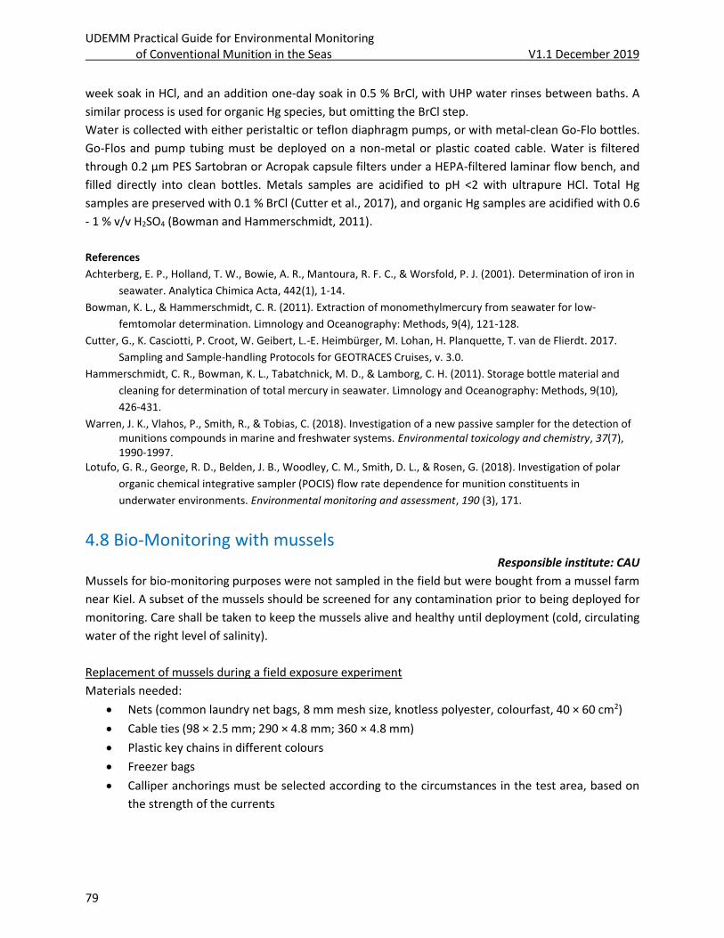
UDEMM Practical Guide for Environmental Monitoring of Conventional Munition in the Seas V1.1 December 2019
79
week soak in HCl, and an addition one-day soak in 0.5 % BrCl, with UHP water rinses between baths. A
similar process is used for organic Hg species, but omitting the BrCl step.
Water is collected with either peristaltic or teflon diaphragm pumps, or with metal-clean Go-Flo bottles.
Go-Flos and pump tubing must be deployed on a non-metal or plastic coated cable. Water is filtered
through 0.2 µm PES Sartobran or Acropak capsule filters under a HEPA-filtered laminar flow bench, and
filled directly into clean bottles. Metals samples are acidified to pH <2 with ultrapure HCl. Total Hg
samples are preserved with 0.1 % BrCl (Cutter et al., 2017), and organic Hg samples are acidified with 0.6
- 1 % v/v H2SO4 (Bowman and Hammerschmidt, 2011).
References
Achterberg, E. P., Holland, T. W., Bowie, A. R., Mantoura, R. F. C., & Worsfold, P. J. (2001). Determination of iron in
seawater. Analytica Chimica Acta, 442(1), 1-14.
Bowman, K. L., & Hammerschmidt, C. R. (2011). Extraction of monomethylmercury from seawater for low‐
femtomolar determination. Limnology and Oceanography: Methods, 9(4), 121-128.
Cutter, G., K. Casciotti, P. Croot, W. Geibert, L.-E. Heimbürger, M. Lohan, H. Planquette, T. van de Flierdt. 2017.
Sampling and Sample-handling Protocols for GEOTRACES Cruises, v. 3.0.
Hammerschmidt, C. R., Bowman, K. L., Tabatchnick, M. D., & Lamborg, C. H. (2011). Storage bottle material and
cleaning for determination of total mercury in seawater. Limnology and Oceanography: Methods, 9(10),
426-431.
Warren, J. K., Vlahos, P., Smith, R., & Tobias, C. (2018). Investigation of a new passive sampler for the detection of munitions compounds in marine and freshwater systems. Environmental toxicology and chemistry, 37(7), 1990-1997.
Lotufo, G. R., George, R. D., Belden, J. B., Woodley, C. M., Smith, D. L., & Rosen, G. (2018). Investigation of polar
organic chemical integrative sampler (POCIS) flow rate dependence for munition constituents in
underwater environments. Environmental monitoring and assessment, 190 (3), 171.
4.8 Bio-Monitoring with mussels Responsible institute: CAU
Mussels for bio-monitoring purposes were not sampled in the field but were bought from a mussel farm
near Kiel. A subset of the mussels should be screened for any contamination prior to being deployed for
monitoring. Care shall be taken to keep the mussels alive and healthy until deployment (cold, circulating
water of the right level of salinity).
Replacement of mussels during a field exposure experiment
Materials needed:
• Nets (common laundry net bags, 8 mm mesh size, knotless polyester, colourfast, 40 × 60 cm2)
• Cable ties (98 × 2.5 mm; 290 × 4.8 mm; 360 × 4.8 mm)
• Plastic key chains in different colours
• Freezer bags
• Calliper anchorings must be selected according to the circumstances in the test area, based on
the strength of the currents
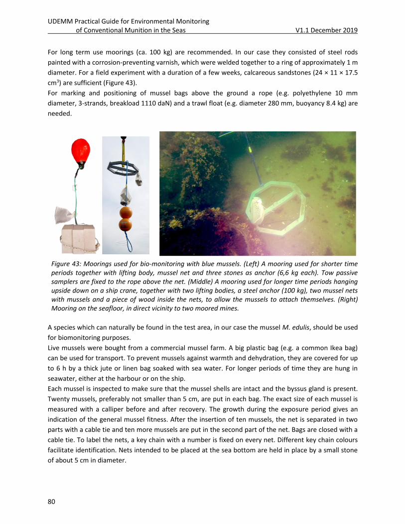
UDEMM Practical Guide for Environmental Monitoring of Conventional Munition in the Seas V1.1 December 2019
80
For long term use moorings (ca. 100 kg) are recommended. In our case they consisted of steel rods
painted with a corrosion-preventing varnish, which were welded together to a ring of approximately 1 m
diameter. For a field experiment with a duration of a few weeks, calcareous sandstones (24 × 11 × 17.5
cm3) are sufficient (Figure 43).
For marking and positioning of mussel bags above the ground a rope (e.g. polyethylene 10 mm
diameter, 3-strands, breakload 1110 daN) and a trawl float (e.g. diameter 280 mm, buoyancy 8.4 kg) are
needed.
Figure 43: Moorings used for bio-monitoring with blue mussels. (Left) A mooring used for shorter time periods together with lifting body, mussel net and three stones as anchor (6,6 kg each). Tow passive samplers are fixed to the rope above the net. (Middle) A mooring used for longer time periods hanging upside down on a ship crane, together with two lifting bodies, a steel anchor (100 kg), two mussel nets with mussels and a piece of wood inside the nets, to allow the mussels to attach themselves. (Right) Mooring on the seafloor, in direct vicinity to two moored mines.
A species which can naturally be found in the test area, in our case the mussel M. edulis, should be used
for biomonitoring purposes.
Live mussels were bought from a commercial mussel farm. A big plastic bag (e.g. a common Ikea bag)
can be used for transport. To prevent mussels against warmth and dehydration, they are covered for up
to 6 h by a thick jute or linen bag soaked with sea water. For longer periods of time they are hung in
seawater, either at the harbour or on the ship.
Each mussel is inspected to make sure that the mussel shells are intact and the byssus gland is present.
Twenty mussels, preferably not smaller than 5 cm, are put in each bag. The exact size of each mussel is
measured with a calliper before and after recovery. The growth during the exposure period gives an
indication of the general mussel fitness. After the insertion of ten mussels, the net is separated in two
parts with a cable tie and ten more mussels are put in the second part of the net. Bags are closed with a
cable tie. To label the nets, a key chain with a number is fixed on every net. Different key chain colours
facilitate identification. Nets intended to be placed at the sea bottom are held in place by a small stone
of about 5 cm in diameter.
UDEMM Practical Guide for Environmental Monitoring of Conventional Munition in the Seas V1.1 December 2019
81
After recovery, the mussels should be unpacked as soon as possible and put in insulated bags on dry ice.
For longer periods of time the mussels may be stored at -20°C in a freezer, until used.
4.9 Chemical analyses of water, sediment and organic matter Responsible institutes: GEOMAR & CAU
4.9.1 Sample preparation
4.9.1.1 Water
Dissolved MCs: Samples were stored at 4°C and pre-concentrated as soon as possible after collection.
Solid phase extraction was used for matrix removal and pre-concentration. Optimal pre-concentration
conditions included a column preconditioning step with 4 mL acetonitrile (ACN) followed by 4 mL MQ-
H2O (gravity flow), sample loading (1 L) at a flow rate of 8 mL min-1 with the automated pre-
concentration system or by gravity, rinsing with 10 mL MQ-H2O under gravity flow, and sample elution
with 3.5 mL ACN. For sample elution, ACN was first loaded onto the column and left for approximately 5
min, prior to elution into a vial via gravity flow. A 1.75 mL sample aliquot was evaporated to near
dryness (ca. 50 µL) under vacuum after addition of 50 µl of MQ-H2O with a centrifugal evaporator. The
evaporite was diluted to 0.5 mL with 50:50 MQ-H2O:MeOH (v/v) and mixed for approximately 20 sec
with a vortexor. Samples were transferred to an amber HPLC vial and kept at 4°C prior to analysis.
Particle-associated MCs: Filter-retained particles are extracted directly in the intact filter cartridges
using 5 mL of LCMS grade acetonitrile. The acetonitrile is allowed to permeate the filter membrane, and
then left in contact for 15 min. The acetonitrile is then forced through the filter into a sample vial.
Samples are diluted to 30 % with MilliQ water, and analysed directly.
4.9.1.2 Mussel Condition Index
To compare general mussel fitness between different groups of exposed mussels, the Condition Index
(CI) is calculated. Before sample preparation the shells and meat are weighed separately. The CI is
calculated as follows: CI = [wet meat weight (g)/shell weight (g)] × 100.
4.9.1.3 Biota - Wet homogenization/extraction
Up to eight mussels are thawed, the whole meat put in a 50 mL polypropylene tube and homogenized
using a T25 Ultra-Turrax. Tissues are aliquoted in 1.0 g portions, put in 50 mL polypropylene tubes and 5
mL acetonitrile are added per tube. Each sample is mixed for 1 min using a vortex mixer. After that,
tubes are centrifuged for 5 min at 3000 rpm (20 °C). Supernatants are decanted and filled up with
acetonitrile to a total volume of 10.0 mL, followed by GC-MS analysis.
4.9.1.4 Sediment and Biota - Lyophilization and dry homogenization/extraction
Sediment and biota samples are frozen and then lyophilized. Biota is ground to a coarse powder using a
stainless steel grinder. For MCs, approximately 10-500 mg of tissue samples are extracted in one or two
millilitres of acetonitrile. The smaller volume of ACN is used when available sample mass is less than 150
mg. Approximately 2 g of sediment are extracted in 10 mL ACN. Samples are sonicated for 15 min, and
extracts filtered through 0.2 µm PTFE syringe filters (Whatman GD/X). Extracts are diluted with MQ-H2O
to 30 % ACN for analysis.
UDEMM Practical Guide for Environmental Monitoring of Conventional Munition in the Seas V1.1 December 2019
82
For metals and Hg analysis extraction follows Hammerschmidt and Fitzgerald (2001) and Tseng et al.
(1997). Briefly, dried solid samples (0.1-1 g dry weight) are placed in 15 mL polypropylene centrifuge
tubes. 8 mL of 4M ultrapure HNO3 is added to the samples and analytes are extracted in an ultrasonic
bath at 55°C for 15 min. Microwave-assisted extraction is also appropriate (Tseng et al., 1997). Samples
are centrifuged, and the supernatant retained for analysis.
4.9.2 Analysis
4.9.2.1 MC analysis by GC-MS
For GC-MS/MS analysis samples were injected in a Trace 1310 gas chromatograph (Thermo Fisher
Scientific Inc., Waltham, MA, USA) and eluted analytes were ionized with electron ionization (EI) or
negative chemical ionization (CI) with methane as the reagent gas and analysed with a TSQ 8000 EVO
Triple Quadrupole Mass Spectrometer (Thermo Fisher Scientific Inc., Waltham, MA, USA) in MRM-mode.
For details, see appendix.
4.9.2.2 MC analysis by LC-ESI-MS
Pre-concentrated MCs from the dissolved phase are analysed in a matrix of 50 % (vol.) LCMS-grade
methanol or 33 % LCMS-grade ACN. Additional method detail is found in Gledhill et al. (2019). Briefly,
samples are analysed with a biocompatible ultra-high performance liquid chromatographic system
(UHPLC, Ultimate 3000, Thermo) consisting of a binary high pressure pump, a temperature controlled
autosampler, a column oven and a UV-visible diode array detector. Analytes are separated using a
150 × 2.1 mm Explosives E2 column. The eluent from the UV detector is injected via a divert valve into a
heated electrospray ionisation source and then into a high resolution quadrapole/orbitrap mass
analyser (HESI-MS, Q Exactive, Thermo). The UHPLC-HESI-MS is controlled with Xcalibur and Chromeleon
software.
4.9.2.3 ICP-MS
Dissolved metals are analysed after automated solid-phase pre-concentration, following Rapp et al.
(2017). Briefly, 10 mL subsamples are buffered to pH 6.4 using ultrapure ammonium acetate, pre-
concentrated on WAKO resin at 3 mL/min, and eluted with 1 mL of ultrapure 1M HNO3. The eluate is
analysed directly by ICPMS. Sediment and tissue extracts are analysed by ICPMS for both metals and Hg.
Dilution of the digest solution may be necessary, to avoid injecting strong acid solutions into the ICPMS.
4.9.2.4 CV-AFS
For total Hg samples are analysed by purge-and-trap thermal desorption CV-AFS (Cutter et al., 2017).
Samples are neutralized with 0.05 % v/v hydroxylamine hydrochloride, reduced with stannous chloride
or sodium borohydride, and the Hg trapped on gold-coated sand columns. Trapped Hg on the column is
desorbed at 600-800 °C, and flushed into a CV-AFS detector for quantification. For Methyl-Hg, the
sample is digested with H2SO4 for 12 h, and buffered to pH 5 with sodium acetate. Methyl-Hg is
ethylated with Na-tetraethylborate, sparged from solution, and trapped on a Tenax column (Bowman
and Hammerschmidt, 2011). The Tenax column is heated to 90 - 250°C, and organic species separated
on an isothermal GC column, pyrolyzed at 600 - 800°C and detected by CV-AFS.
UDEMM Practical Guide for Environmental Monitoring of Conventional Munition in the Seas V1.1 December 2019
83
References
Bowman, K. L., & Hammerschmidt, C. R. (2011). Extraction of monomethylmercury from seawater for low‐
femtomolar determination. Limnology and Oceanography: Methods, 9(4), 121-128.
Cutter, G., K. Casciotti, P. Croot, W. Geibert, L.-E. Heimbürger, M. Lohan, H. Planquette, T. van de Flierdt. 2017.
Sampling and Sample-handling Protocols for GEOTRACES Cruises, v. 3.0.
Hammerschmidt, C. R., & Fitzgerald, W. F. (2001). Formation of artifact methylmercury during extraction from a
sediment reference material. Analytical chemistry, 73(24), 5930-5936.
Rapp, I., Schlosser, C., Rusiecka, D., Gledhill, M., & Achterberg, E. P. (2017). Automated preconcentration of Fe, Zn,
Cu, Ni, Cd, Pb, Co, and Mn in seawater with analysis using high-resolution sector field inductively-coupled
plasma mass spectrometry. Analytica chimica acta, 976, 1-13.
Tseng, C. M., DE DIEGO, A. L. B. E. R. T. O., Martin, F. M., & Donard, O. F. (1997). Rapid and quantitative
microwave-assisted recovery of methylmercury from standard reference sediments. Journal of analytical atomic
spectrometry, 12(6), 629-635.
UDEMM Practical Guide for Environmental Monitoring of Conventional Munition in the Seas V1.1 December 2019
84
5. Appendix 5.1 Analysis of nitroaromatic compounds in mussel tissue (blue
mussels)
Materials needed:
Standard compounds (acquired from AccuStandard Inc., New Haven, USA)
• 2,4,6-trinitrotoluene (TNT) (1 mg/mL)
• 2-amino-4,6-dinitrotoluene (2-ADNT) (1 mg/mL)
• 4-amino-2,6-dinitrotoluene (4-ADNT) (1 mg/mL)
• 2,4-diamino-6-nitrotoluene (2,4-DANT) (0.1 mg/mL)
• 2,6-diamino-4-nitrotoluene (2,6-DANT) (0.1 mg/mL)
Acetonitrile, gradient grade
Conical polypropylene tubes, 50 mL
Homogenizer (Ultra-Turrax®, Ika Works Inc., Staufen im Breisgau, Germany)
Vortex mixer (Vf2, Ika Works Inc., Staufen im Breisgau, Germany)
Centrifuge, capable to process 50 mL conical tubes (Heraeus Megafuge 11R, Thermo Fisher Scientific
Inc., Waltham, MA, USA)
Sample preparation
Up to eight mussels are thawed, the whole meat put in a 50 mL polypropylene tube and homogenized
using a T25 Ultra-Turrax®. Tissues are aliquoted in 1.0 g portions, put in 50 mL polypropylene tubes and
5 mL acetonitrile are added per tube. Each sample is mixed for 1 min using a vortex mixer. After that,
tubes are centrifuged for 5 min at 3000 g (20 °C). Supernatants are decanted and filled up with
acetonitrile to a total volume of 10.0 mL, followed by GC-MS analysis.
GC-MS/MS analysis
Short column
The detection limit (signal to noise ratio > 3) for TNT, 4-ADNT and 2-ADNT was 0.5 ng/g wet weight in
case of the 15 m column. For GC-MS/MS analysis one microliter of the samples is injected with a
splitless liner in a Trace 1310 Gas Chromatograph (Thermo Fisher Scientific Inc., Waltham, MA, USA) and
analytes are separated on a TG-SQC GC column (15 m × 0.25 mm × 0.25 μm, Thermo Fisher Scientific
Inc., Waltham, MA, USA). Helium is used as carrier gas with a carrier flow rate of 1.5 mL/min and a split
flow rate of 20 mL/min. The oven temperature program is as follows (Figure 44):
1. 1 min at 120°C
2. heating to 220°C with a heating rate of 30°C/min
3. heating to 300°C with a heating rate of 50°C/min
4. 300°C held for 0.5 min
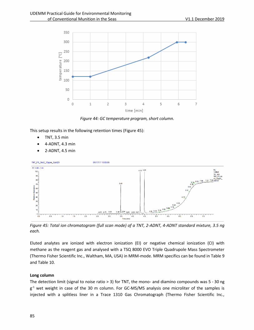
UDEMM Practical Guide for Environmental Monitoring of Conventional Munition in the Seas V1.1 December 2019
85
Figure 44: GC temperature program, short column.
This setup results in the following retention times (Figure 45):
• TNT, 3.5 min
• 4-ADNT, 4.3 min
• 2-ADNT, 4.5 min
Figure 45: Total ion chromatogram (full scan mode) of a TNT, 2-ADNT, 4-ADNT standard mixture, 3.5 ng each.
Eluted analytes are ionized with electron ionization (EI) or negative chemical ionization (CI) with
methane as the reagent gas and analysed with a TSQ 8000 EVO Triple Quadrupole Mass Spectrometer
(Thermo Fisher Scientific Inc., Waltham, MA, USA) in MRM-mode. MRM specifics can be found in Table 9
and Table 10.
Long column
The detection limit (signal to noise ratio > 3) for TNT, the mono- and diamino compounds was 5 - 30 ng
g-1 wet weight in case of the 30 m column. For GC-MS/MS analysis one microliter of the samples is
injected with a splitless liner in a Trace 1310 Gas Chromatograph (Thermo Fisher Scientific Inc.,
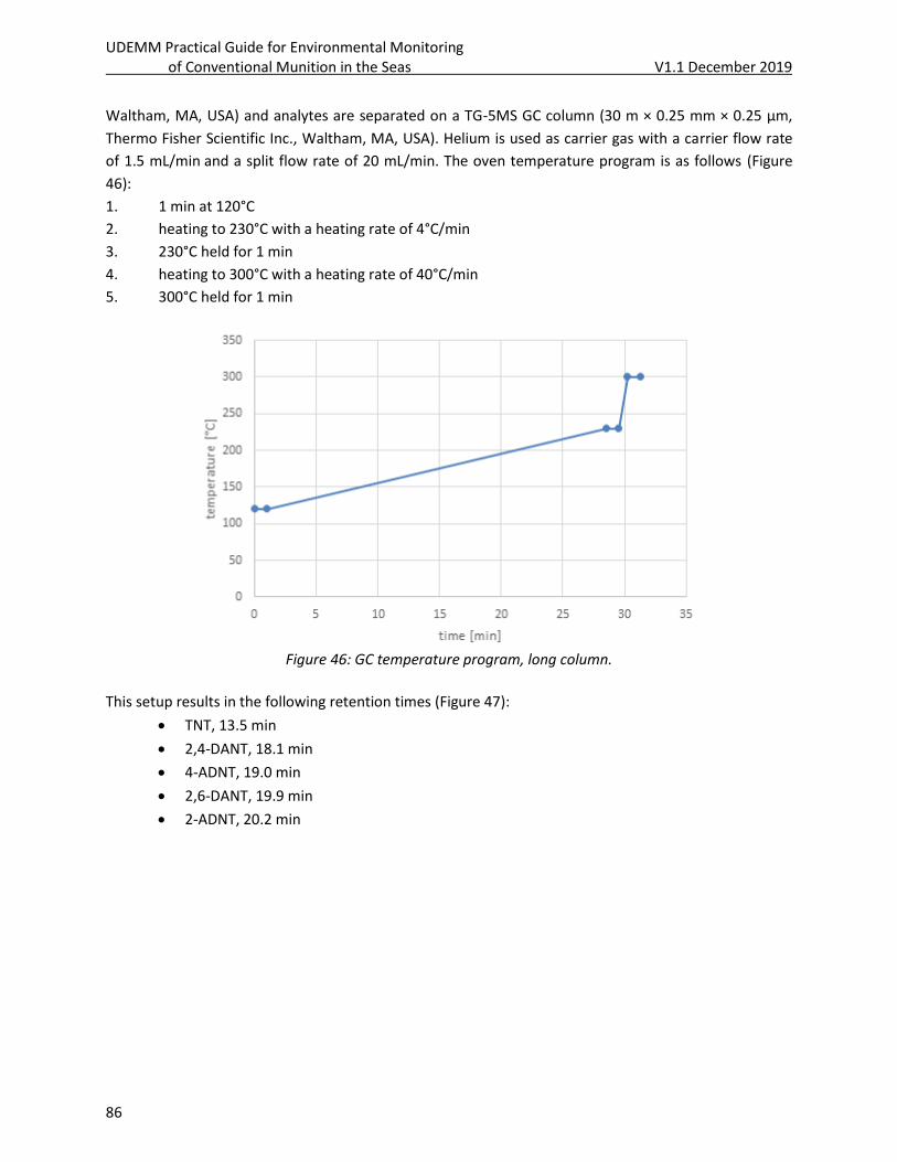
UDEMM Practical Guide for Environmental Monitoring of Conventional Munition in the Seas V1.1 December 2019
86
Waltham, MA, USA) and analytes are separated on a TG-5MS GC column (30 m × 0.25 mm × 0.25 μm,
Thermo Fisher Scientific Inc., Waltham, MA, USA). Helium is used as carrier gas with a carrier flow rate
of 1.5 mL/min and a split flow rate of 20 mL/min. The oven temperature program is as follows (Figure
46):
1. 1 min at 120°C
2. heating to 230°C with a heating rate of 4°C/min
3. 230°C held for 1 min
4. heating to 300°C with a heating rate of 40°C/min
5. 300°C held for 1 min
Figure 46: GC temperature program, long column.
This setup results in the following retention times (Figure 47):
• TNT, 13.5 min
• 2,4-DANT, 18.1 min
• 4-ADNT, 19.0 min
• 2,6-DANT, 19.9 min
• 2-ADNT, 20.2 min
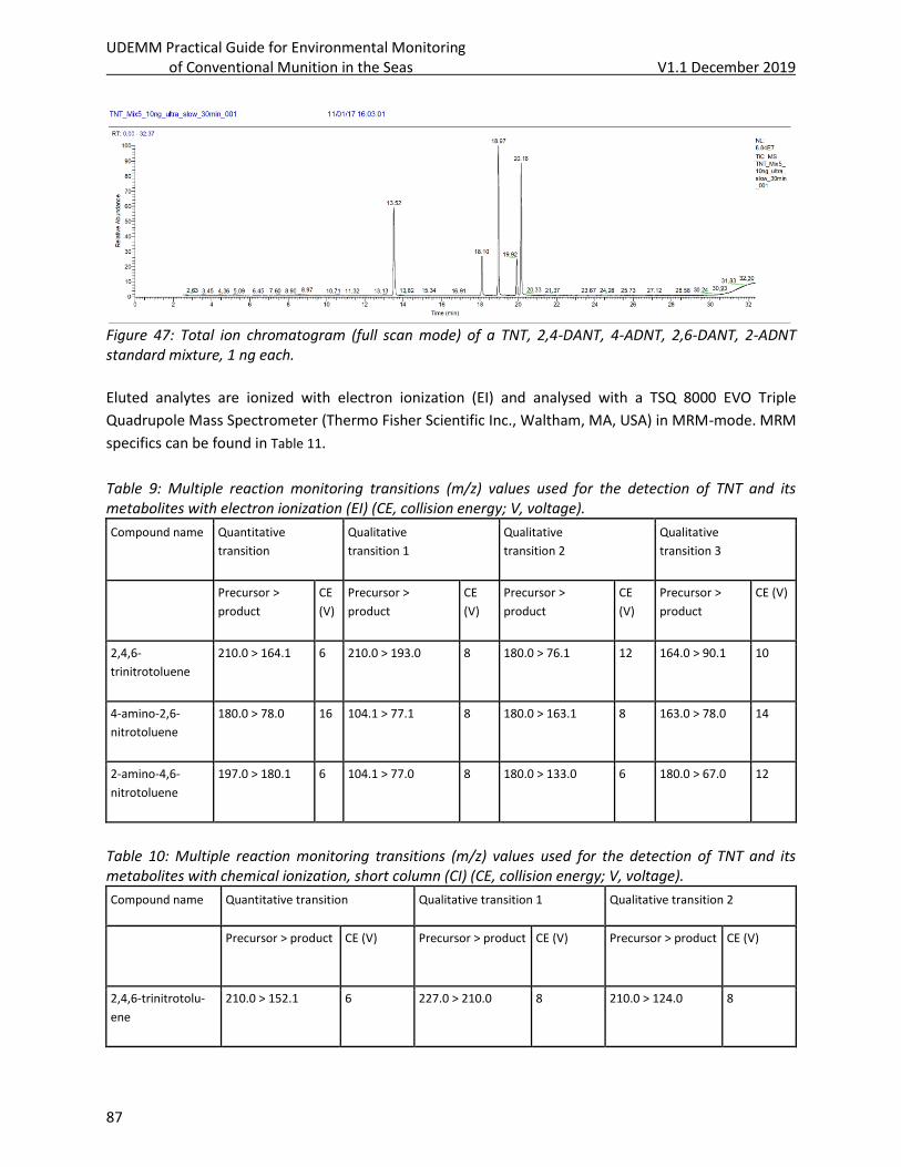
UDEMM Practical Guide for Environmental Monitoring of Conventional Munition in the Seas V1.1 December 2019
87
Figure 47: Total ion chromatogram (full scan mode) of a TNT, 2,4-DANT, 4-ADNT, 2,6-DANT, 2-ADNT standard mixture, 1 ng each.
Eluted analytes are ionized with electron ionization (EI) and analysed with a TSQ 8000 EVO Triple
Quadrupole Mass Spectrometer (Thermo Fisher Scientific Inc., Waltham, MA, USA) in MRM-mode. MRM
specifics can be found in Table 11.
Table 9: Multiple reaction monitoring transitions (m/z) values used for the detection of TNT and its metabolites with electron ionization (EI) (CE, collision energy; V, voltage).
Compound name Quantitative
transition
Qualitative
transition 1
Qualitative
transition 2
Qualitative
transition 3
Precursor >
product
CE
(V)
Precursor >
product
CE
(V)
Precursor >
product
CE
(V)
Precursor >
product
CE (V)
2,4,6-
trinitrotoluene
210.0 > 164.1 6 210.0 > 193.0 8 180.0 > 76.1 12 164.0 > 90.1 10
4-amino-2,6-
nitrotoluene
180.0 > 78.0 16 104.1 > 77.1 8 180.0 > 163.1 8 163.0 > 78.0 14
2-amino-4,6-
nitrotoluene
197.0 > 180.1 6 104.1 > 77.0 8 180.0 > 133.0 6 180.0 > 67.0 12
Table 10: Multiple reaction monitoring transitions (m/z) values used for the detection of TNT and its metabolites with chemical ionization, short column (CI) (CE, collision energy; V, voltage).
Compound name Quantitative transition Qualitative transition 1 Qualitative transition 2
Precursor > product CE (V) Precursor > product CE (V) Precursor > product CE (V)
2,4,6-trinitrotolu-
ene
210.0 > 152.1 6 227.0 > 210.0 8 210.0 > 124.0 8
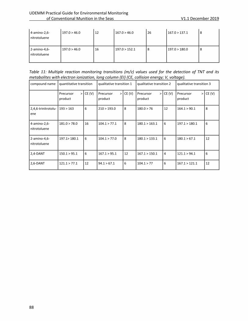
UDEMM Practical Guide for Environmental Monitoring of Conventional Munition in the Seas V1.1 December 2019
88
4-amino-2,6-
nitrotoluene
197.0 > 46.0 12 167.0 > 46.0 26 167.0 > 137.1 8
2-amino-4,6-
nitrotoluene
197.0 > 46.0 16 197.0 > 152.1 8 197.0 > 180.0 8
Table 11: Multiple reaction monitoring transitions (m/z) values used for the detection of TNT and its metabolites with electron ionization, long column (EI) (CE, collision energy; V, voltage).
compound name quantitative transition qualitative transition 1 qualitative transition 2 qualitative transition 3
Precursor >
product
CE (V) Precursor >
product
CE (V) Precursor >
product
CE (V) Precursor >
product
CE (V)
2,4,6-trinitrotolu-
ene
193 > 163 6 210 > 193.0 8 180.0 > 76 12 164.1 > 90.1 8
4-amino-2,6-
nitrotoluene
181.0 > 78.0 16 104.1 > 77.1 8 180.1 > 163.1 6 197.1 > 180.1 6
2-amino-4,6-
nitrotoluene
197.1> 180.1 6 104.1 > 77.0 8 180.1 > 133.1 6 180.1 > 67.1 12
2,4-DANT 150.1 > 95.1 6 167.1 > 95.1 12 167.1 > 150.1 4 121.1 > 94.1 6
2,6-DANT 121.1 > 77.1 12 94.1 > 67.1 6 104.1 > 77 6 167.1 > 121.1 12
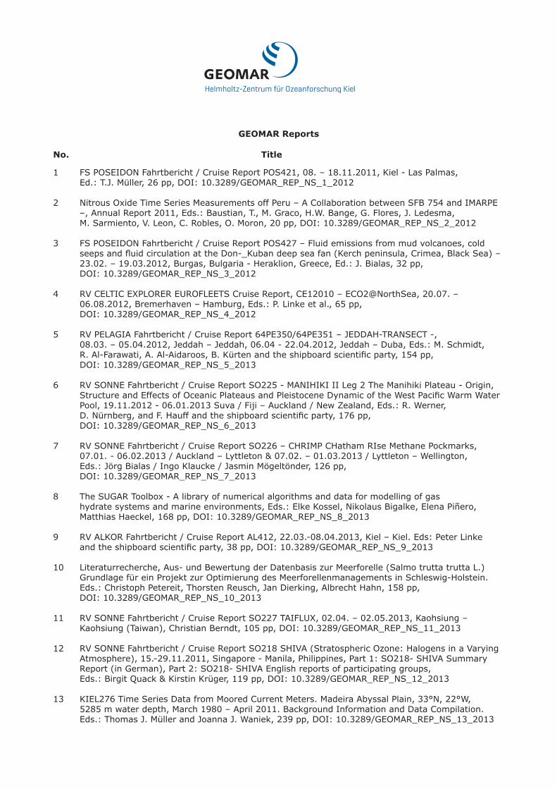
GEOMAR Reports
No. Title
1 FS POSEIDON Fahrtbericht / Cruise Report POS421, 08. – 18.11.2011, Kiel - Las Palmas, Ed.: T.J. Müller, 26 pp, DOI: 10.3289/GEOMAR_REP_NS_1_2012
2 Nitrous Oxide Time Series Measurements off Peru – A Collaboration between SFB 754 and IMARPE –, Annual Report 2011, Eds.: Baustian, T., M. Graco, H.W. Bange, G. Flores, J. Ledesma, M. Sarmiento, V. Leon, C. Robles, O. Moron, 20 pp, DOI: 10.3289/GEOMAR_REP_NS_2_2012
3 FS POSEIDON Fahrtbericht / Cruise Report POS427 – Fluid emissions from mud volcanoes, cold seeps and fluid circulation at the Don-_Kuban deep sea fan (Kerch peninsula, Crimea, Black Sea) – 23.02. – 19.03.2012, Burgas, Bulgaria - Heraklion, Greece, Ed.: J. Bialas, 32 pp,
DOI: 10.3289/GEOMAR_REP_NS_3_2012
4 RV CELTIC EXPLORER EUROFLEETS Cruise Report, CE12010 – ECO2@NorthSea, 20.07. – 06.08.2012, Bremerhaven – Hamburg, Eds.: P. Linke et al., 65 pp,
DOI: 10.3289/GEOMAR_REP_NS_4_2012
5 RV PELAGIA Fahrtbericht / Cruise Report 64PE350/64PE351 – JEDDAH-TRANSECT -, 08.03. – 05.04.2012, Jeddah – Jeddah, 06.04 - 22.04.2012, Jeddah – Duba, Eds.: M. Schmidt, R. Al-Farawati, A. Al-Aidaroos, B. Kürten and the shipboard scientific party, 154 pp,
DOI: 10.3289/GEOMAR_REP_NS_5_2013
6 RV SONNE Fahrtbericht / Cruise Report SO225 - MANIHIKI II Leg 2 The Manihiki Plateau - Origin, Structure and Effects of Oceanic Plateaus and Pleistocene Dynamic of the West Pacific Warm Water Pool, 19.11.2012 - 06.01.2013 Suva / Fiji – Auckland / New Zealand, Eds.: R. Werner, D. Nürnberg, and F. Hauff and the shipboard scientific party, 176 pp,
DOI: 10.3289/GEOMAR_REP_NS_6_2013
7 RV SONNE Fahrtbericht / Cruise Report SO226 – CHRIMP CHatham RIse Methane Pockmarks, 07.01. - 06.02.2013 / Auckland – Lyttleton & 07.02. – 01.03.2013 / Lyttleton – Wellington, Eds.: Jörg Bialas / Ingo Klaucke / Jasmin Mögeltönder, 126 pp, DOI: 10.3289/GEOMAR_REP_NS_7_2013
8 The SUGAR Toolbox - A library of numerical algorithms and data for modelling of gas hydrate systems and marine environments, Eds.: Elke Kossel, Nikolaus Bigalke, Elena Piñero, Matthias Haeckel, 168 pp, DOI: 10.3289/GEOMAR_REP_NS_8_2013
9 RV ALKOR Fahrtbericht / Cruise Report AL412, 22.03.-08.04.2013, Kiel – Kiel. Eds: Peter Linke and the shipboard scientific party, 38 pp, DOI: 10.3289/GEOMAR_REP_NS_9_2013
10 Literaturrecherche, Aus- und Bewertung der Datenbasis zur Meerforelle (Salmo trutta trutta L.) Grundlage für ein Projekt zur Optimierung des Meerforellenmanagements in Schleswig-Holstein. Eds.: Christoph Petereit, Thorsten Reusch, Jan Dierking, Albrecht Hahn, 158 pp, DOI: 10.3289/GEOMAR_REP_NS_10_2013
11 RV SONNE Fahrtbericht / Cruise Report SO227 TAIFLUX, 02.04. – 02.05.2013, Kaohsiung – Kaohsiung (Taiwan), Christian Berndt, 105 pp, DOI: 10.3289/GEOMAR_REP_NS_11_2013
12 RV SONNE Fahrtbericht / Cruise Report SO218 SHIVA (Stratospheric Ozone: Halogens in a Varying Atmosphere), 15.-29.11.2011, Singapore - Manila, Philippines, Part 1: SO218- SHIVA Summary Report (in German), Part 2: SO218- SHIVA English reports of participating groups, Eds.: Birgit Quack & Kirstin Krüger, 119 pp, DOI: 10.3289/GEOMAR_REP_NS_12_2013
13 KIEL276 Time Series Data from Moored Current Meters. Madeira Abyssal Plain, 33°N, 22°W, 5285 m water depth, March 1980 – April 2011. Background Information and Data Compilation. Eds.: Thomas J. Müller and Joanna J. Waniek, 239 pp, DOI: 10.3289/GEOMAR_REP_NS_13_2013
GEOMAR Reports
No. Title
14 RV POSEIDON Fahrtbericht / Cruise Report POS457: ICELAND HAZARDS Volcanic Risks from Iceland and Climate Change:The Late Quaternary to Anthropogene Development Reykjavík / Iceland – Galway / Ireland, 7.-22. August 2013. Eds.: Reinhard Werner, Dirk Nürnberg and the shipboard scientific party, 88 pp, DOI: 10.3289/GEOMAR_REP_NS_14_2014
15 RV MARIA S. MERIAN Fahrtbericht / Cruise Report MSM-34 / 1 & 2, SUGAR Site, Varna – Varna, 06.12.13 – 16.01.14. Eds: Jörg Bialas, Ingo Klaucke, Matthias Haeckel, 111 pp, DOI: 10.3289/GEOMAR_REP_NS_15_2014
16 RV POSEIDON Fahrtbericht / Cruise Report POS 442, “AUVinTYS” High-resolution geological inves-tigations of hydrothermal sites in the Tyrrhenian Sea using the AUV “Abyss”, 31.10. – 09.11.12, Messina – Messina, Ed.: Sven Petersen, 32 pp, DOI: 10.3289/GEOMAR_REP_NS_16_2014
17 RV SONNE, Fahrtbericht / Cruise Report, SO 234/1, “SPACES”: Science or the Assessment of Complex Earth System Processes, 22.06. – 06.07.2014, Walvis Bay / Namibia - Durban / South Africa, Eds.: Reinhard Werner and Hans-Joachim Wagner and the shipbord scientific party, 44 pp, DOI: 10.3289/GEOMAR_REP_NS_17_2014
18 RV POSEIDON Fahrtbericht / Cruise Report POS 453 & 458, “COMM3D”, Crustal Structure and Ocean Mixing observed with 3D Seismic Measurements, 20.05. – 12.06.2013 (POS453), Galway, Ireland – Vigo, Portugal, 24.09. – 17.10.2013 (POS458), Vigo, Portugal – Vigo, Portugal, Eds.: Cord Papenberg and Dirk Klaeschen, 66 pp, DOI: 10.3289/GEOMAR_REP_NS_18_2014
19 RV POSEIDON, Fahrtbericht / Cruise Report, POS469, “PANAREA”, 02. – 22.05.2014, (Bari, Italy – Malaga, Spain) & Panarea shallow-water diving campaign, 10. – 19.05.2014, Ed.: Peter Linke, 55 pp, DOI: 10.3289/GEOMAR_REP_NS_19_2014
20 RV SONNE Fahrtbericht / Cruise Report SO234-2, 08.-20.07.2014, Durban, -South Africa - Port Louis, Mauritius, Eds.: Kirstin Krüger, Birgit Quack and Christa Marandino, 95 pp, DOI: 10.3289/GEOMAR_REP_NS_20_2014
21 RV SONNE Fahrtbericht / Cruise Report SO235, 23.07.-07.08.2014, Port Louis, Mauritius to Malé, Maldives, Eds.: Kirstin Krüger, Birgit Quack and Christa Marandino, 76 pp, DOI: 10.3289/GEOMAR_REP_NS_21_2014
22 RV SONNE Fahrtbericht / Cruise Report SO233 WALVIS II, 14.05-21.06.2014, Cape Town, South Africa - Walvis Bay, Namibia, Eds.: Kaj Hoernle, Reinhard Werner, and Carsten Lüter, 153 pp, DOI: 10.3289/GEOMAR_REP_NS_22_2014
23 RV SONNE Fahrtbericht / Cruise Report SO237 Vema-TRANSIT Bathymetry of the Vema-Fracture Zone and Puerto Rico TRench and Abyssal AtlaNtic BiodiverSITy Study, Las Palmas (Spain) - Santo Domingo (Dom. Rep.) 14.12.14 - 26.01.15, Ed.: Colin W. Devey, 130 pp, DOI: 10.3289/GEOMAR_REP_NS_23_2015
24 RV POSEIDON Fahrtbericht / Cruise Report POS430, POS440, POS460 & POS467 Seismic Hazards to the Southwest of Portugal; POS430 - La-Seyne-sur-Mer - Portimao (7.4. - 14.4.2012), POS440 - Lisbon - Faro (12.10. - 19.10.2012), POS460 - Funchal - Portimao (5.10. - 14.10.2013), POS467 - Funchal - Portimao (21.3. - 27.3.2014), Ed.: Ingo Grevemeyer, 43 pp, DOI: 10.3289/GEOMAR_REP_NS_24_2015
25 RV SONNE Fahrtbericht / Cruise Report SO239, EcoResponse Assessing the Ecology, Connectivity and Resilience of Polymetallic Nodule Field Systems, Balboa (Panama) – Manzanillo (Mexico), 11.03. -30.04.2015, Eds.: Pedro Martínez Arbizu and Matthias Haeckel, 204 pp, DOI: 10.3289/GEOMAR_REP_NS_25_2015
GEOMAR Reports
No. Title
26 RV SONNE Fahrtbericht / Cruise Report SO242-1, JPI OCEANS Ecological Aspects of Deep-Sea Mining, DISCOL Revisited, Guayaquil - Guayaquil (Equador), 29.07.-25.08.2015, Ed.: Jens Greinert, 290 pp, DOI: 10.3289/GEOMAR_REP_NS_26_2015
27 RV SONNE Fahrtbericht / Cruise Report SO242-2, JPI OCEANS Ecological Aspects of Deep-Sea Mining DISCOL Revisited, Guayaquil - Guayaquil (Equador), 28.08.-01.10.2015, Ed.: Antje Boetius, 552 pp, DOI: 10.3289/GEOMAR_REP_NS_27_2015
28 RV POSEIDON Fahrtbericht / Cruise Report POS493, AUV DEDAVE Test Cruise, Las Palmas - Las Palmas (Spain), 26.01.-01.02.2016, Ed.: Klas Lackschewitz, 17 pp, DOI: 10.3289/GEOMAR_REP_NS_28_2016
29 Integrated German Indian Ocean Study (IGIOS) - From the seafloor to the atmosphere - A possible German contribution to the International Indian Ocean Expedition 2 (IIOE-2) programme – A Science Prospectus, Eds.: Bange, H.W. , E.P. Achterberg, W. Bach, C. Beier, C. Berndt, A. Biastoch, G. Bohrmann, R. Czeschel, M. Dengler, B. Gaye, K. Haase, H. Herrmann, J. Lelieveld, M. Mohtadi, T. Rixen, R. Schneider, U. Schwarz-Schampera, J. Segschneider, M. Visbeck, M. Voß, and J. Williams, 77pp, DOI: 10.3289/GEOMAR_REP_NS_29_2016
30 RV SONNE Fahrtbericht / Cruise Report SO249, BERING – Origin and Evolution of the Bering Sea: An Integrated Geochronological, Volcanological, Petrological and Geochemical Approach, Leg 1: Dutch Harbor (U.S.A.) - Petropavlovsk-Kamchatsky (Russia), 05.06.2016-15.07.2016, Leg 2: Petropavlovsk-Kamchatsky (Russia) - Tomakomai (Japan), 16.07.2016-14.08.2016, Eds.: Reinhard Werner, et al., DOI: 10.3289/GEOMAR_REP_NS_30_2016
31 RV POSEIDON Fahrtbericht / Cruise Report POS494/2, HIERROSEIS Leg 2: Assessment of the Ongoing Magmatic-Hydrothermal Discharge of the El Hierro Submarine Volcano, Canary Islands by the Submersible JAGO, Valverde – Las Palmas (Spain), 07.02.-15.02.2016, Eds.: Hannington, M.D. and Shipboard Scientific Party, DOI: 10.3289/GEOMAR_REP_NS_31_2016
32 RV METEOR Fahrtbericht / Cruise Report M127, Extended Version, Metal fluxes and Resource Potential at the Slow-spreading TAG Midocean Ridge Segment (26°N, MAR) – Blue Mining@Sea, Bridgetown (Barbados) – Ponta Delgada (Portugal) 25.05.-28.06.2016, Eds.: Petersen, S. and Shipboard Scientific Party, DOI: 10.3289/GEOMAR_REP_NS_32_2016
33 RV SONNE Fahrtbericht /Cruise Report SO244/1, GeoSEA: Geodetic Earthquake Observatory on the Seafloor, Antofagasta (Chile) – Antofagasta (Chile), 31.10.-24.11.2015, Eds.: Jan Behrmann, Ingo Klaucke, Michal Stipp, Jacob Geersen and Scientific Crew SO244/1, DOI: 10.3289/GEOMAR_REP_NS_33_2016
34 RV SONNE Fahrtbericht /Cruise Report SO244/2, GeoSEA: Geodetic Earthquake Observatory on the Seafloor, Antofagasta (Chile) – Antofagasta (Chile), 27.11.-13.12.2015, Eds.: Heidrun Kopp, Dietrich Lange, Katrin Hannemann, Anne Krabbenhoeft, Florian Petersen, Anina Timmermann and Scientific Crew SO244/2, DOI: 10.3289/GEOMAR_REP_NS_34_2016
35 RV SONNE Fahrtbericht /Cruise Report SO255, VITIAZ – The Life Cycle of the Vitiaz-Kermadec Arc / Backarc System: from Arc Initiation to Splitting and Backarc Basin Formation, Auckland (New Zealand) - Auckland (New Zealand), 02.03.-14.04.2017, Eds.: Kaj Hoernle, Folkmar Hauff, and Reinhard Werner with contributions from cruise participants, DOI: 10.3289/GEOMAR_REP_NS_35_2017
GEOMAR Reports
No. Title
36 RV POSEIDON Fahrtbericht /Cruise Report POS515, CALVADOS - CALabrian arc mud VolcAnoes: Deep Origin and internal Structure, Dubrovnik (Croatia) – Catania (Italy), 18.06.-13.07.2017, Eds.: M. Riedel, J. Bialas, A. Krabbenhoeft, V. Bähre, F. Beeck, O. Candoni, M. Kühn, S. Muff, J. Rindfleisch, N. Stange, DOI: 10.3289/GEOMAR_REP_NS_36_2017
37 RV MARIA S. MERIAN Fahrtbericht /Cruise Report MSM63, PERMO, Southampton – Southampton (U.K.), 29.04.-25.05.2017, Eds.: Christian Berndt and Judith Elger with contributions from cruise participants C. Böttner, R.Gehrmann, J. Karstens, S. Muff, B. Pitcairn, B. Schramm, A. Lichtschlag, A.-M. Völsch, DOI: 10.3289/GEOMAR_REP_NS_37_2017
38 RV SONNE Fahrtbericht /Cruise Report SO258/1, INGON: The Indian - Antarctic Break-up Engima, Fremantle (Australia) - Colombo (Sri Lanka), 07.06.-09.07.2017, 29.04.-25.05.2017, Eds.: Reinhard Werner, Hans-Joachim Wagner, and Folkmar Hauff with contributions from cruise participants, DOI: 10.3289/GEOMAR_REP_NS_38_2017
39 RV POSEIDON Fahrtbericht /Cruise Report POS509, ElectroPal 2: Geophysical investigations of sediment hosted massive sulfide deposits on the Palinuro Volcanic Complex in the Tyrrhenian Sea, Malaga (Spain) – Catania (Italy), 15.02.-03.03.2017, Ed.: Sebastian Hölz, DOI: 10.3289/GEOMAR_REP_NS_39_2017
40 RV POSEIDON Fahrtbericht /Cruise Report POS518, Baseline Study for the Environmental Moni-toring of Subseafloor CO2 Storage Operations, Leg 1: Bremerhaven – Bremerhaven (Germany), 25.09.-11.10.2017, Leg 2: Bremerhaven – Kiel (Germany), 12.10.-28.10.2017, Eds.: Peter Linke and Matthias Haeckel, DOI: 10.3289/GEOMAR_REP_NS_40_2018
41 RV MARIA S. MERIAN Fahrtbericht /Cruise Report MSM71, LOBSTER: Ligurian Ocean Bottom Seismology and Tectonics Research, Las Palmas (Spain) – Heraklion (Greece), 07.02.-27.02.2018, Eds.: H. Kopp, D. Lange, M. Thorwart, A. Paul, A. Dannowski, F. Petersen, C. Aubert, F. Beek, A. Beniest, S. Besançon, A. Brotzer, G. Caielli, W. Crawford, M. Deen, C. Lehmann, K. Marquardt, M. Neckel, L. Papanagnou, B. Schramm, P. Schröder, K.-P. Steffen, F. Wolf, Y. Xia, DOI: 10.3289/GEOMAR_REP_NS_41_2018
42 RV METEOR Fahrtbericht /Cruise Report M143, SLOGARO: Slope failures and active gas expulsion along the Romanian margin – investigating relations to gas hydrate distribution, Varna (Romania) – Heraklion (Greece), 12.12.-22.12.2017, Eds.: M. Riedel, F. Gausepohl, I. Gazis, L. Hähnel, M. Kampmeier, P. Urban, J. Bialas, DOI: 10.3289/GEOMAR_REP_NS_42_2018
43 RV POSEIDON Fahrtbericht /Cruise Report POS510, ANYDROS: Rifting and Hydrothermal Activity in the Cyclades Back-arc Basin, Catania (Italy) – Heraklion (Greece), 06.03.-29.03.2017, Ed.: M.D. Hannington, DOI: 10.3289/GEOMAR_REP_NS_43_2018
44 RV POSEIDON Fahrtbericht /Cruise Report POS524, GrimseyEM: Geophysical and geological investigations in the vicinity of the Grimsey Hydrothermal Field offshore Northern Iceland for the assessment of the geothermal potential and the exploration for potential mineralizations within the seafloor, Reykjavik (Iceland) – Bergen (Norway), 7.6 - 26.6.2018, Eds.: Sebastian Hölz and Sofia Martins, DOI: 10.3289/GEOMAR_REP_NS_44_2018
45 RV POSEIDON Fahrtbericht /Cruise Report POS527, Baseline Study for the Environmental Monitoring of Subseafloor CO2 Storage Operations, Kiel – Kiel (Germany), 15.8. - 3.9.2018, Eds.: Eric Achterberg and Mario Esposito, DOI: 10.3289/GEOMAR_REP_NS_45_2018
GEOMAR Reports
No. Title
46 RV SONNE Fahrtbericht /Cruise Report SO264, SONNE-EMPEROR: The Plio/Pleistocene to Holocene development of the pelagic North Pacific from surface to depth – assessing its role for the global carbon budget and Earth´s climate, Suva (Fiji) – Yokohama (Japan), 30.6. – 24.8.2018 Ed.: Dirk Nürnberg, DOI: 10.3289/GEOMAR_REP_NS_46_2018
47 RV SONNE Fahrtbericht /Cruise Report SO265, SHATSKY EVOLUTION: Evolution of the Shatsky Rise Hotspot System, Yokohama (Japan) – Kaohsiung (Taiwan), 26.08. – 11.10.2018, Eds.: Jörg Geldmacher, Reinhard Werner, and Folkmar Hauff with contributions from cruise participants, DOI: 10.3289/GEOMAR_REP_NS_47_2018
48 RV MARIA S. MERIAN Fahrtbericht /Cruise Report MSM78, PERMO 2, Edinburgh – Edinburgh (U.K.), 16.10. – 25.10.2018, Eds.: Jens Karstens, Christoph Böttner, Mike Edwards, Ismael Falcon-Suarez, Anita Flohr, Rachael James, Anna Lichtschlag, Doris Maicher, Iain Pheasant, Ben Roche, Bettina Schramm, Michael Wilson, DOI: 10.3289/GEOMAR_REP_NS_48_2019
49 RV SONNE Fahrtbericht /Cruise Report SO267, ARCHIMEDES I: Arc Rifting, Metallogeny and Micro-plate Evolution – an Integrated Geodynamic, Magmatic and Hydrothermal Study of the Fonualei Rift System, NE Lau Basin, Suva (Fiji) – Suva (Fiji), 11.12.2018 – 26.01.2019, Eds.: Mark Hannington, Heidrun Kopp, Michael Schnabel, DOI: 10.3289/GEOMAR_REP_NS_49_2019
50 RV Pelagia Fahrtbericht /Cruise Report 64PE-445, SALTAX: Geomorphology and geophysics of sub-marine salt flows in the Red Sea Rift, Limassol (Cyprus) – Safaga (Egypt), 27.08. – 21.09.2018, Eds.: Nico Augustin, Neil C. Mitchell, Froukje M. van der Zwan & Scientific Shipboard Party, DOI: 10.3289/GEOMAR_REP_NS_50_2019
51 RV POSEIDON Fahrtbericht /Cruise Report POS526, SeASOM: Semi-Autonomous Subsurface Optical Monitoring for methane seepage and cold-water coral studies in the North Sea, Bergen (Norway) – Doggerbank (Netherlands) – Hirtshals (Denmark) – Tisler (Norway) – Kiel (Germany), 23.07. – 11.08.2018, Eds.: Jens Greinert, Tim Schoening, DOI: 10.3289/GEOMAR_REP_NS_51_2019
52 RV POSEIDON Fahrtbericht /Cruise Report POS534, STEMM-CCS: Strategies for Environmental Monitoring of Marine Carbon Capture and Storage, Leg 1: Kiel (Germany) – Aberdeen (United Kingdom), 01.05. – 22.05.2019, Leg 2: Aberdeen (United Kingdom) – Bremerhaven (Germany), 23.05. – 29.05.2019, Ed.: Mark Schmidt, DOI: 10.3289/GEOMAR_REP_NS_52_2019
53 RV POSEIDON Fahrtbericht /Cruise Report POS535, Loki2GrimseyEM: Geophysical and geological investigations of massive sulfides at and in the vicinity of Loki’s Castle (Norway) and similar experiments around the Grimsey Hydrothermal Field (Iceland) for the assessment of the geo thermal potential and the exploration for potential mineralizations within the seafloor, Akureyri (Iceland) – Bremerhaven (Germany), 09.06 – 03.07.2019, Eds.: Sebastian Hölz, Amir Haroon and Sofia Martins, DOI: 10.3289/GEOMAR_REP_NS_53_2019
54 Practical Guide for Environmental Monitoring of Conventional Munitions in the Seas, Results from the BMBF funded project UDEMM “Umweltmonitoring für die Delaboration von Munition im Meer” Ed.: Jens Greinert, DOI: 10.3289/GEOMAR_REP_NS_54_2019
For GEOMAR Reports, please visit:https://oceanrep.geomar.de/view/series/GEOMAR_Report.html
Reports of the former IFM-GEOMAR series can be found under:https://oceanrep.geomar.de/view/series/IFM-GEOMAR_Report.html
Das GEOMAR Helmholtz-Zentrum für Ozeanforschung Kielist Mitglied der Helmholtz-Gemeinschaft
Deutscher Forschungszentren e.V.
The GEOMAR Helmholtz Centre for Ocean Research Kielis a member of the Helmholtz Association of
German Research Centres
Helmholtz-Zentrum für Ozeanforschung Kiel / Helmholtz Centre for Ocean Research KielGEOMARDienstgebäude Westufer / West Shore BuildingDüsternbrooker Weg 20D-24105 KielGermany
Helmholtz-Zentrum für Ozeanforschung Kiel / Helmholtz Centre for Ocean Research KielGEOMARDienstgebäude Ostufer / East Shore BuildingWischhofstr. 1-3D-24148 KielGermany
Tel.: +49 431 600-0Fax: +49 431 600-2805www.geomar.de