Embed Size (px)
Citation preview

Sohail AhmedSudhaharan Thankiah
Radek MachánMartin Hof
Andrew H. A. ClaytonGraham Wright
Jean-Baptiste SibaritaThomas Korte
Andreas Herrmann
FLUORESCENCEPRACTICAL MANUAL FOR
MICROSCOPYTECHNIQUES

3chapter

Frequency-domain Fluorescence Lifetime Imaging Microscopy (FD-FLIM)
Andrew H.A. ClaytonCentre for Micro-Photonics, Faculty of Science,
Engineering and Technology, Swinburne University of Technology, Hawthorn, Victoria, Australia
Index1. Principle and Theory ........................................................................................................... 3
How is the Fluorescence Waveform Detected? ............................................................. 42. Instrumentation ................................................................................................................... 4
Light Sources ................................................................................................................. 5Detectors ........................................................................................................................ 5Microscope ..................................................................................................................... 5Software ......................................................................................................................... 6
3. Method................................................................................................................................ 8Sample: General Considerations ................................................................................... 8Sample: Specific Examples ............................................................................................ 8
4. Image Acquisition ............................................................................................................... 95. Data Analysis ...................................................................................................................... 9
Histogram Analysis of Regions of Interest ...................................................................... 9Polar Plot Analysis .......................................................................................................... 9Interpretation of Results ................................................................................................. 9Artefacts and Trouble shooting .................................................................................... 10
4. Technique Overview ..........................................................................................................11Applications ...................................................................................................................11Limitations .................................................................................................................... 12
References and Further Reading ........................................................................................ 13Appendix: Lifetime Acquisition and Analysis from Lambert Manual ..................................... 15

3 Frequency-domain Fluorescence Lifetime Imaging Microscopy (FD-FLIM) | 3-4
1. Principle and Theory
The excited-state lifetime is defined as the mean time a molecule spends in the excited-state. The ex-cited-state lifetime of a fluorescent probe provides a robust and sensitive measure of the probe’s en-vironment. It can change in response to environ-mental changes such as micro-polarity and pH. It can also change when a suitable molecule in nearby by a process called fluorescence resonance energy transfer (FRET). In the latter case the excited-state lifetime of the fluorophore decreases in a characteris-tic fashion with distance between the two molecules. The excited-state lifetime, unlike intensity, is a kinetic quantity and as such largely independent of factors such as concentration or optical path length. When the lifetime is resolved spatially and presented as an image we refer to this as a fluorescence lifetime image. The technology used to collect and interpret a fluorescence lifetime image is called fluorescence lifetime imaging microscopy (FLIM).The principle behind measuring excited-state life-times is to excite the molecule of interest and measure the response of that molecule to that ex-citation. In the time-domain the excitation is pulsed and the response is a convolution of that pulse with the excited-state decay of the molecule-usually for short pulses the emission appears as an exponen-tially-decaying signal, see Figure 1.The frequency-domain technique is less intuitive
than the time-domain analogue because we are often used to thinking of decay processes in time. But in fact our circadian rhythms operate in the frequen-cy-domain. We are used to waking and sleeping with a given period or frequency which is controlled by the periodicity of night and day. We can also excite a collection of molecules with light that is continu-ous but intensity modulated with a given frequency. If the molecules emit photons immediately after ex-citation, then the emission will appear with the same frequency as the excitation and the shape of the emitted waveform will be identical to the shape of the excitation waveform. This is the situation of zero-life-time. However, if there is a delay between excitation and emission, due to a finite excited-state lifetime, then the emitted waveform will be shifted in phase. We call this a phase shift or a phase lag. A human analogy is jet lag. The light and day cycle is shifted in phase due to air travel from different time zones and this is out of phase with our internal circadian clock. In the frequency-domain two parameters are obtained from the detected waveforms that related to the lifetime or lifetime distribution. Not surprisingly, the phase shift, is related to the lifetime of the excited state. As implied from the above discussion, the smaller the phase difference between excitation and emission, the shorter the lifetime of the excited state. Another property of a waveform is the modulation. A time-delay between excitation and emission causes a loss of modulation or demodulation of the fluores-cence signal. That is the longer the excited-state lifetime the greater the demodulation.Figure 2 contains a schematic that illustrates and defines modulation and phase-shift.For a single exponential decaying system character-ised by a lifetime, t, the intensity remaining, I(t), after time, t is given by the expression.
(1)
The corresponding phase (f) in FD-FLIM is given by the expression,
(2)
And the modulation is given by the expression,
(3)
In equations (2) and (3) w is the modulation frequency.The lifetime determined from the phase (equation 2) is often referred to as the “phase lifetime” and the corresponding lifetime determined from the modula-tion (equation 3) is called the “modulation lifetime”. For single exponential processes the phase lifetime is equal to the modulation lifetimes. For non-expo-nential decay processes (those involving sums of
Figure 1 Schematic representation of the principle behind time-re-solved fluorescence measurement techniques. Top: Delta excitation pulse (blue line) excites a fluorescent sample (cylinder) and this sample emits fluorescence with exponential time decay (red line). Middle: If the excitation pulse (blue line) is broad, the response to the excitation appears as broadened emission decay (red-line). Bottom: Sinusoidal-modulated excitation (blue line) and resulting sinusoidal emission (red line). Note the change in shape of the fluo-rescence due to the finite excited state decay of the fluorophore.

3 Frequency-domain Fluorescence Lifetime Imaging Microscopy (FD-FLIM) | 3-5
exponential functions) the phase lifetime and mod-ulation lifetimes are not equal. Expressions for more complex decaying systems (non-exponential time decays or sums of exponential decays) are given elsewhere. Although determination of these more complex models is possible using multi-frequen-cy methods, in practise measurements of FLIM on biological samples are performed at a single mod-ulation frequency. For questions of biological impor-tance one is usually more interested in a change in the emission decay of a sample through FRET or changes in microenvironment. Importantly, changes in the excited-state lifetime of the fluorophore are inferred through a change in the phase and modula-tion of the emission. Later we will see a representa-tion of this phase and modulation that is particularly convenient and useful for interpretation of FLIM ex-periments.
How is the Fluorescence Waveform Detected?Before we go into the “nuts and bolts” of the instrumen-tation, it is important to consider how the sinusoidal fluorescent waveform is detected. As can be gleaned from equations 2 and 3, to measure lifetimes on the order of nanoseconds requires modulation frequen-cies of the order of reciprocal lifetimes, i.e. 10-100 MHz. The excitation must be modulated at high fre-quency and we require the phase and modulation of the emitted high-frequency signal. The determi-nation of the emitted fluorescence signal waveform can be achieved using heterodyne or homodyne detection. In heterodyne detection a high-frequen-
cy signal is transformed into a low frequency signal. In homodyne detection the high frequency signal is transformed into a static phase-dependent signal. In both techniques the fluorescence signal is multiplied with a reference waveform derived from a common modulation source. In the heterodyne technique the gain of the detector is modulated at a slightly different frequency to the frequency of the excitation source. The result of mixing the emission at one frequency with the gain at a slightly different frequency is a new waveform with low frequency and identical phase and modulation to the original (high-frequency) emitted waveform. Time-sampling of this low frequency waveform and subsequent Fourier analysis recovers the phase and modulation information.In the homodyne method the gain of the detector is modulated at exactly the same frequency as the ex-citation. This gives a filtered signal that depends only on the phase difference between the emission and the reference waveform. This signal may be sampled by shifting the phase between the detector and the excitation. Repeating this process generates a waveform at each pixel of the image which contains the phase and modulation information.
2. Instrumentation
A schematic of a typical wide-field FD-FLIM is shown in Figure 3. This system is built around a research grade microscope with the light source directed
A
B
Excitaion
��
�
Time
Emission
Inte
nsity
Figure 2 Schematic representation of excitation and emission waveforms in FD-FLIM. Blue line represents the excitation waveform with average signal intensity A and waveform amplitude B. The red-line represents the waveform of the emission. Due to the finite lifetime of the excited-state, the emission waveform is shifted in phase (j) and de-modulated, that is the amplitude of the emission waveform (b) divided by the average signal (a) is reduced compared to the modulation of the excitation (B/A).

3 Frequency-domain Fluorescence Lifetime Imaging Microscopy (FD-FLIM) | 3-6
through the back of the microscope and the detector mounted onto an emission side-port (microscope not shown). The difference between a conventional microscope and an FD-FLIM microscope lies in the detector. The heart of this system is the micro-chan-nel plate image intensifier which serves as the mixing device in homo-dyne or heterodyne detection. The gain of the intensifier is modulated at high-frequen-cy under control of the signal generator and this waveform is essentially mixed in the detector with the emission signal waveform that emerges from the microscope. The signal generator sends an identical frequency signal to the light source which provides the modulated excitation waveform. The CCD camera is a detector that provides a digital 2D representation of the image that impinges on the MCP phosphor. The computer contains software that controls the fre-quency of modulation and shifts the phase between the MCP and light source, reads the images from the CCD camera, and computes lifetime images.
Light SourcesIn FD-FLIM any repetitive waveform that excites the molecule of interest is required. For typical lifetimes of 1-10 ns one requires 10-100 MHz frequencies (see equation (2)). Continuous lasers can be used in combination with acousto-optic or electo-optic modulators to provide the periodic, modulated ex-citation waveform. Pulsed laser systems such as Ti-Sa lasers, have also been used and provide the added advantage of two-photon excitation. Direct electrical modulation of light-emitting diodes and
laser diodes has been demonstrated. For example, in the Lambert Instruments LIFA system modulated LEDs or modulated laser diodes are used as the ex-citation source.
DetectorsThe detection of the emitted fluorescence signal waveform can be carried out in a number of ways depending on the configuration of the microscope (scanning or wide-field) or whether the detection is homo-dyne or heterodyne. When scanning is used (either stage scanning with fixed laser or laser scanning with fixed stage) the emission is focussed onto a single detector, usually a photomultiplier tube, an avalanche photodiode or a micro-channel plate detector and the signal is timed with the position of the scanning stage or laser to extract an image. In wide-field FD-FLIM instruments the whole field is illuminated and the image focussed onto an area detector such as a micro-channel plate image inten-sifier and a charge-coupled device camera. MicroscopeMost FLIM systems are built on a research grade flu-orescence microscope. The objective lens is an es-sential optical element that provides the magnifica-tion needed to see objects on the (sub) micron scale. The delivery of the excitation light and the handling of the fluorescence emission differ depending on the type of microscope and the desired imaging modality but most systems employ a dichroic mirror to reflect emitted light to the detector and excitation
LI²CAM-Xcamera
C-mount
Em
D
Lamphousingwith LED
Personal Computer
LIFAcontrol unit
Microscope
ModulationSignals USB
USB 2.0 portsEx
Figure 3 Schematic representation of the LIFA wide-field FD-FLIM. Components are discussed in the main text. (Diagram from the Lambert Instruments LIFA manual).

3 Frequency-domain Fluorescence Lifetime Imaging Microscopy (FD-FLIM) | 3-7
and emission filters to select excitation and emission wavelengths. In confocal systems, hardware is needed to deliver and raster scan a laser beam to the sample and a pin-hole between the emission and the detector is utilised to reject out of focus light. In wide-field systems, no extra hardware is needed aside from the excitation source, signal generator and image inten-sifier and charge-coupled device camera.
SoftwareThe output of a FD-FLIM experiment is a stack of images that represents a sinusoidal function at every pixel. There are a number of steps required before the raw data stacks can be converted into a lifetime image. These steps include;
1. Background correction. This can be performed in a number of ways. A small region outside the sample is interactively selected and the average intensity value from that region in each phase image is subtracted. Alternatively, an image is collected with the excitation source blocked and this image is subtracted from each phase-de-pendent image. In-cell background correction is more challenging but can be done in some circumstances as a post processing step (see details later).
2. Correction for photobleaching. All fluorophores photobleach to some extent and if not taken into account FD-FLIM values can be distorted. The traditional photobleaching correction is to record
phase images in one sequence then re-re-cord the phase images in reverse sequence. Averaging the two sequences of images corrects for linear photobleaching. A more recent inno-vation utilised permuting the recording order so that the phase steps are not sequentially increasing but rather pseudo-random in record-ing order. This second method is advantageous because it obviates the requirement of recording two series of phase stacks.
3. Correction for instrumental phase shift and de-modulation. The instrument has an intrinsic phase bias and a demodulation. In the time-do-main this is called the instrument response function and represents the finite width of the laser pulse and the timing jitter in the detector and the electronics. In the frequency domain, the light source, electronics and detector all contributed to a finite demodulation and phase of the instrument. This is readily corrected by recording a phase stack of images with a refer-ence of known lifetime (fluorescein, rhodamine 6G are good examples). Because the reference stacks are from solutions with no microscop-ic detail spatial averaging is usually performed on these solution images before the phase and modulation images are extracted.
4. Calculation of phase and modulation images of sample and reference. Once the image stacks representing corrected images are stored in memory, the phase and modulation images are required because they contain information about
Figure 4 A Representative lifetime histogram. Plot of the number of pixels versus fluorescence lifetime (in nanoseconds). The large number of pixels in an FD-FLIM image leads to large sample sizes and consequently well-defined lifetime distributions. Even small lifetime shifts of the order of 100ps or less can be readily discerned. B Representative lifetime image. Note the regions in blue that denote very short lifetimes (1.6 ns) compared with the yellow-orange regions (2-2.1 ns).

3 Frequency-domain Fluorescence Lifetime Imaging Microscopy (FD-FLIM) | 3-8
the excited-state decay processes at hand. The phase-stacks can be processed efficiently using Fourier Transform methods, namely discrete sine and cosine transformations, which in turn can be manipulated to deliver the required phase and modulations at every pixel location in an image. Direct fitting to a sinusoidal function is also a possibility, which yields the required phase and modulation.
Once the phase and modulation are known then phase lifetime and modulation lifetime images are created (see equations 2 and 3). The lifetime images can be color-coded to aid visualisation of regions with different lifetime. An alternative representation is in terms of histograms. The lifetime is binned into dif-ferent values on the horizontal axis and the number of pixels in each bin is plotted on the vertical axis. An example of a lifetime histogram is displayed in Figure 4A and an example of a color-coded FLIM image is shown in Figure 4B.A very useful and convenient visualisation of data is achieved with a plot called the polar plot (or phasor or AB-plot). The phase and modulation is transformed into point on a 2D plot. For a given phase, f, and modulation, M, the coordinates of the point on the polar plot are;
(4)
(5)
For a single species the time-decay of the fluores-cence emission is represented by a single point on the polar plot at location (Mcosf,Msinf). If the emission decay is single exponential, the phasor will be located somewhere on a semi-circle circum-scribed by the points (0,0), (1/2,1/2) and (1,0) and the position on that semi-circle reveals the actual lifetime value. For more complex heterogenous decays the phasor will be located inside the semi-cir-cle. For excited-state reactions involving sensitised acceptor emission or solvent relaxation, the phasor will be located outside the semi-circle. The polar plot can also reveal data from different experiments (different samples, or same sample different conditions) or data as a function of image location or time or any other hidden variable. The re-sulting spread of data is often referred to as a polar plot trajectory. The use of the polar plot has many advantages. (a) Irrespective of the complexity of the fluorescence
decay, any fluorophore can be represented as a single point in the polar plot.
(b) Mixtures between different species are repre-sented by the vector sum of the phasors of the
M
�
B
A
�1= 2.5 ns �
2= 1.5 ns
�2= 1.0 ns
�2= 0.5 ns
0 0.2 0.4 0.6 0.8 10
0.2
0.4
0.6
0.8
1
Figure 5 Polar plot or AB-plot. The red dot represents one fluorescent species with a given fluorescence decay profile. The length of the red-line is the modulation of the emission and angle subtended by the red-line is the phase. Selected single-exponential lifetimes are denoted by the black dots on the dashed semi-circle. Binary mixtures of different lifetime species are denoted by the chords linking the dots. A,B,M and j are defined in the text.
3 Frequency-domain Fluorescence Lifetime Imaging Microscopy (FD-FLIM) | 3-9
individual species. All possible mixing combi-nations fall on a line connecting the individual species. For the mixture of three species the mixture falls inside a triangle. For N-species this will be a polygon with N-vertexes.
(c) FRET experiments can also be simulated taking into account background fluorescence and contri-butions from non-FRET states.
(d) Data from only one modulation frequency is required.
(e) Analysis of a potentially complex multi-exponen-tial decay problem is reduced to simple rules of vector algebra and trigonometry.
3. Method
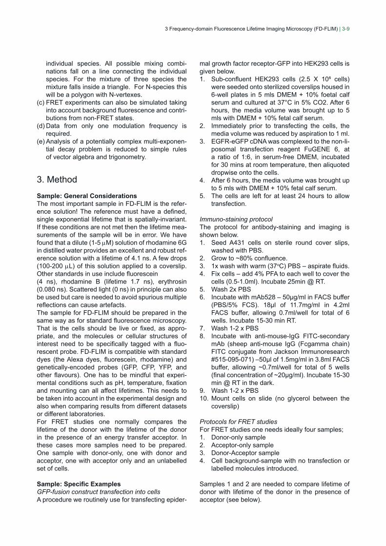
Sample: General ConsiderationsThe most important sample in FD-FLIM is the refer-ence solution! The reference must have a defined, single exponential lifetime that is spatially-invariant. If these conditions are not met then the lifetime mea-surements of the sample will be in error. We have found that a dilute (1-5 mM) solution of rhodamine 6G in distilled water provides an excellent and robust ref-erence solution with a lifetime of 4.1 ns. A few drops (100-200 mL) of this solution applied to a coverslip. Other standards in use include fluorescein (4 ns), rhodamine B (lifetime 1.7 ns), erythrosin (0.080 ns). Scattered light (0 ns) in principle can also be used but care is needed to avoid spurious multiple reflections can cause artefacts.The sample for FD-FLIM should be prepared in the same way as for standard fluorescence microscopy. That is the cells should be live or fixed, as appro-priate, and the molecules or cellular structures of interest need to be specifically tagged with a fluo-rescent probe. FD-FLIM is compatible with standard dyes (the Alexa dyes, fluorescein, rhodamine) and genetically-encoded probes (GFP, CFP, YFP, and other flavours). One has to be mindful that experi-mental conditions such as pH, temperature, fixation and mounting can all affect lifetimes. This needs to be taken into account in the experimental design and also when comparing results from different datasets or different laboratories.For FRET studies one normally compares the lifetime of the donor with the lifetime of the donor in the presence of an energy transfer acceptor. In these cases more samples need to be prepared. One sample with donor-only, one with donor and acceptor, one with acceptor only and an unlabelled set of cells.
Sample: Specific ExamplesGFP-fusion construct transfection into cellsA procedure we routinely use for transfecting epider-
mal growth factor receptor-GFP into HEK293 cells is given below. 1. Sub-confluent HEK293 cells (2.5 X 10⁵ cells)
were seeded onto sterilized coverslips housed in 6-well plates in 5 mls DMEM + 10% foetal calf serum and cultured at 37°C in 5% CO2. After 6 hours, the media volume was brought up to 5 mls with DMEM + 10% fetal calf serum.
2. Immediately prior to transfecting the cells, the media volume was reduced by aspiration to 1 ml.
3. EGFR-eGFP cDNA was complexed to the non-li-posomal transfection reagent FuGENE 6, at a ratio of 1:6, in serum-free DMEM, incubated for 30 mins at room temperature, then aliquoted dropwise onto the cells.
4. After 6 hours, the media volume was brought up to 5 mls with DMEM + 10% fetal calf serum.
5. The cells are left for at least 24 hours to allow transfection.
Immuno-staining protocolThe protocol for antibody-staining and imaging is shown below.1. Seed A431 cells on sterile round cover slips,
washed with PBS.2. Grow to ~80% confluence.3. 1x wash with warm (37oC) PBS – aspirate fluids.4. Fix cells – add 4% PFA to each well to cover the
cells (0.5-1.0ml). Incubate 25min @ RT.5. Wash 2x PBS6. Incubate with mAb528 – 50µg/ml in FACS buffer
(PBS/5% FCS). 18µl of 11.7mg/ml in 4.2ml FACS buffer, allowing 0.7ml/well for total of 6 wells. Incubate 15-30 min RT.
7. Wash 1-2 x PBS8. Incubate with anti-mouse-IgG FITC-secondary
mAb (sheep anti-mouse IgG (Fcgamma chain) FITC conjugate from Jackson Immunoresearch #515-095-071) –50µl of 1.5mg/ml in 3.8ml FACS buffer, allowing ~0.7ml/well for total of 5 wells (final concentration of ~20µg/ml). Incubate 15-30 min @ RT in the dark.
9. Wash 1-2 x PBS10. Mount cells on slide (no glycerol between the
coverslip)
Protocols for FRET studiesFor FRET studies one needs ideally four samples;1. Donor-only sample2. Acceptor-only sample3. Donor-Acceptor sample4. Cell background-sample with no transfection or
labelled molecules introduced.
Samples 1 and 2 are needed to compare lifetime of donor with lifetime of the donor in the presence of acceptor (see below).

3 Frequency-domain Fluorescence Lifetime Imaging Microscopy (FD-FLIM) | 3-10
Samples 2 and 3 can be used to determine FRET through sensitized emission (see below). For donor-detected FRET studies sample 2 ensures no spectral bleed-through from acceptor into the donor channel.Sample 4 is to correct the data for background fluo-rescence signal.
4. Image Acquisition
The reader is directed to the Appendix provided by Lambert Instruments on the operation of the LIFA in-strument and obtaining a lifetime image.
5. Data Analysis
The lifetime image takes a bit of getting used to. It is a map of kinetic processes not the intensity or concentration of species as in normal fluorescence microscopy. As a consequence lifetime images can sometimes appear to have less contrast than a flu-orescence intensity image. Careful analysis and display of lifetime images can provide improved in-terpretation.
Histogram Analysis of Regions of InterestSpectroscopists are used to measuring absorption or emission spectra and measuring shifts in spectra. Lifetimes can be displayed in a similar fashion using histograms- a plot of the no. of pixels versus lifetime. Differences in lifetime between different regions of interest of the same image can be revealed by plotting the lifetime histograms of these regions of interest. Using the ROI tools one can select succes-sive regions, which will be numbered 1,2,3 etc. Then going to the statistics tab tick the boxes correspond-ing to the lifetime histogram and the ROI number. A color-coded histogram will appear in the window. The statistics function also provides information on the mean, standard deviation and the number of pixels in the ROI. The histogram analysis can also be applied to different experiments. For example in FRET one compares the lifetime of cells containing a donor with cells containing a donor and acceptor. A shift in the donor histogram to lower lifetime values in the presence of acceptor indicates FRET from the donor to the acceptor.
Polar Plot AnalysisAnother way of visualising a FLIM experiment is to use the polar plot. This can be accessed using the polar plot tab in the LIFA software or alternatively one can use Enrico Gratton’s Globals for Images software. As mentioned before the polar plot rep-resents the phase and modulation values of an
image on a two-dimensional graph. For images the polar plots usually appear as a cloud of points instead of a single point. A selection tool is used to point to specific regions of the polar plot and pixels with these phase and modulation characteristics are highlighted onto the intensity image.
Interpretation of ResultsTests of statistical significanceFor cell biophysical studies, where biological variabil-ity is the rule, statistical tests are an important way of testing whether two sets of observations are signifi-cant or insignificant. The simplest implementation is to analyse 20-50 cells (number of observations, N¹) from one treatment and 20-50 cells (number of ob-servations, N2) from another treatment and compute the corresponding mean phase lifetimes (x1 and x2) and variances (s1 and s2) in the phase lifetime from each treatment dataset. The t-value, which provides a measure of whether the mean values from each dataset are significantly different, is given by the expression,
(6)
The number of degrees of freedom is given by N1+N2-2. Using the number of degrees of freedom and the t-value, a t-table can be examined to deter-mine the significance level of the t-value. For example if 10 cells per treatment condition is measured, the number of degrees of freedom is 18. Inspection of a t-table reveals that for t-values greater than 2.1 the means of the two datasets are significantly different at the 95% significance level.
Background MixingFor cells containing a high level of fluorescence label background fluorescence is usually ignored in FD-FLIM. However as meaningful, biologically-rele-vant studies demand protein expression at physio-logical levels background fluorescence can become an inevitable component of the detected emission. There are generally two types of background. Off-cell background arises from camera offset, room lights, immersion oil, buffers and cover-slips. This type of background can be examined by selection of regions that do not contain cells and subtracted or taken into account in analysis. Cellular autofluorescence is the other source of background and arrises from native (not extrinsically-labelled) molecules contained within the cell eg flavins, collagen etc. This type of fluorescence must be measured in unstained cells before it can be subtracted.The effect of background mixing into the (desired) sample is given by the simple equations,
3 Frequency-domain Fluorescence Lifetime Imaging Microscopy (FD-FLIM) | 3-11
(7)
(8)
Where A and B are the sine and cosine components of the phasor (defined above), and a is the fraction-al fluorescence contribution of the sample emission to the total emission. Equations (7) and (8) can be applied to cell populations, single cells, or at the pixel level. Significant background mixing can be visual-ised in an FD-FLIM image from the polar plot as an elongated cloud of points that begins at (B,A) sample and stretches out to (B,A) background.
FRET or no-FRET?Arguably FD-FLIM is of greatest use in FRET appli-cations for detecting interactions (or conformational changes) between labelled biological macromol-ecules. In FRET excitation of the donor molecule results in non-radiative transfer of energy to the acceptor molecule. If the acceptor is fluorescent it can emit a fluorescence photon. The requirements for FRET are restrictive. The spectral properties of the fluorophores, the orientation between the flu-orophores and the distance are important determi-nants on the efficiency of the FRET process. These aspects are discussed in detail elsewhere. Detection and measurement of FRET by FD-FLIM is relatively straightforward but depends on the exper-imental design. The measurement method is a con-sequence of the photo-physics of the FRET process itself. FRET induced donor lifetime quenching in FD-FLIMFRET adds a non-radiative decay channel to the excited state of the donor. As a consequence FRET decreases the lifetime of the donor molecule in the presence of the acceptor. To detect FRET one measures the lifetime of the donor in the absence of the acceptor (td) and then measures the donor lifetime in the presence of the acceptor (tda). The FRET Efficiency, E, can be computed with the relation,
(9)
The donor lifetime can be determined from a sample containing the donor-only (with no acceptor). Alternatively, the donor-only sample can be prepared from the donor-acceptor sample photo-chemically by photobleaching the acceptor (see acceptor pho-tobleaching chapter). It is very important that in the donor lifetime method the donor is uniquely excited and the emission represents the emission from the donor only. In FD-FLIM lifetime is often the phase lifetime or modulation lifetime. The FRET can also
be calculated using the polar plot and is visualised as a movement of the donor phasor in a clockwise direction along the universal-circle. Methods exist for using the polar plot to analyse FRET in the presence of background emission or in the situation of variable amounts of FRET and non-FRET states. The reader is referred to the publi-cations for more detailed accounts.
Sensitized EmissionFRET results in a delayed emission from the acceptor fluorophore because the initially excited donor transfer energy is transferred (albeit invisible, non-radiatively) to the acceptor. This delay gives an additional phase shift to the acceptor emission (over that associated with the normal excitation and emission from the acceptor). This extra phase can cause an effect known as lifetime inversion, that is the lifetime calculated from the modulation becomes less than the lifetime calculated from the phase. This effect also causes the phasor of the acceptor to move in a counter-clockwise movement outside the semi-circle of the polar plot.
Artefacts and Trouble shooting PhotobleachingPhotobleaching can dramatically distort lifetime mea-surements and in some cases cause an inversion of modulation and phase lifetimes even for simple fluo-rophores. Reducing the excitation intensity and mea-surement times can reduce photobleaching. When photobleaching is unavoidable, pseudo-random phase recording can help reduce the effects of photo-bleaching on lifetime measurements. Consideration of background is needed if photobleaching deterio-rates signal to background levels.
RoomlightRoomlight adds a DC signal to the data. This sys-tematically causes a demodulation of the signal and will distort the lifetime computed from the modulation (i.e. the modulation lifetime will increase). The phase lifetime will not be effected for pure DC signal back-ground. This can be visualised in the polar plot as a line that connects the origin (0,0) to the fluorescence signal. This can be eliminated by turning off the light, covering the sample, or ensuring a background cor-rection image is recorded and subtracted from the phase stacks.
Sample MovementAn FD-FLIM image is a single image derived from several individual images obtained at different times (or different phase steps). An implicit assumption is that there is no movement during image acquisition or perhaps more precisely that the concentration dis-tribution of fluorophores in the image is time invari-

3 Frequency-domain Fluorescence Lifetime Imaging Microscopy (FD-FLIM) | 3-12
ant during the FLIM acquisition. This is often a good assumption (where fluxes in the cell ensure pseu-do-steady-state) or cells are fixed. However, in some cases “comets” can appear in the lifetime images and correspondingly, streaks in the polar plot. These are due to motion of a small number of particles in the image. Whole cell motion will give the effect of shadowing whereby there is a distinctive gradient of high to low lifetime. Motions of a large number of particles will broaden lifetime histograms and cause a blooming of polar plots. In some selected cases this is useful for determining translational diffusion coefficients23. Stabilising the sample and decreas-ing exposure times is the best way to reduce these effects.
Instrument DriftDrift can sometimes occur due to lack of temperature stabilisation on LEDs or AOMS or electronics. If left unchecked, drift can give erroneous impressions of time-dependent biological phenomena or give erratic results. The simplest way of diagnosing and cor-recting drift is to measure a lifetime standard or any stable sample periodically. Small lifetime fluctuations (<0.1 ns) are probably due to random fluctuations.However, any monotonic change in the lifetime of the standard is evidence for drift. A good way to avoid drift is to carry out drift tests during instrument warm up until stability is confirmed. We have found drift to be a rare problem with our set-up with stability of better than 50 ps over a period of hours. Another way of safe-guarding against drift is by permuting sample collection order so that the same sample or reference is collected at several dif-ferent times.
Fixation, AntifadeWe have found that fixation can alter the lifetime of a YFP-tagged cell surface receptor and more an-ecdotal evidence suggests it can effect lifetimes of GFP-tagged proteins. The exact reason for this phe-nomenon is not currently known but it is important to understand that the lifetime of a fluorophore in living cells is not necessarily the same as in fixed cells. Antifade has also been anecdotally attributed to lifetime changes. Because the composition and quantity of antifade may vary from batch to batch or sample to sample it is not recommended to use this with FLIM experiments.
TemperatureMost cell studies are carried out a 4 degrees centi-grade, 37 degrees centigrade or ambient tempera-ture (often undefined). The excited-state lifetimes of nearly all organic fluorophores depend on tempera-ture with a decrease in lifetime with increasing tem-perature. Where possible it is preferable to control
the temperature or at least note the ambient tem-perature at the time of the measurements.
Polarisation EffectsFor molecules excited with polarised light, the time-dependent detected emission depends on the excited-state lifetime, the rotational motion of the flu-orophore and the emission collection geometry. This can be useful for measuring rotational dynamics of fluorophores. However this effect can also perturb lifetime measurements. Use of a polariser in the excitation (or a laser which is polarised) and an analyser in the emission path oriented at the magic angle (54.7 degrees) is the traditional way to exclude polarisation artefacts in time-resolved spectroscopy. This approach is rarely employed in FLIM probably because of the reduction in attendant signal. Instead, lasers are sent through polarisation scrambling fibres to produce excitation light that is not linear-ly-polarised. Unpolarised light sources from lamps or LEDS also reduces but does not guarantee complete removal of the effects of polarisation on FLIM mea-surements.
NoiseNoise is not really an artefact but a reality of the mea-surement process. Clearly a trade-off exists between reducing photo-bleaching and reducing effects of movement, which requires use of low excitation and fast acquisition, and collection of enough emission photons to ensure nicely resolved FLIM images. The signal to noise ratio can be increased by using av-eraging or increasing the exposure time. Increasing the averaging or exposure time by a factor of N will increase the signal to noise ratio by a factor of √N. An alternative approach, for advanced users, is to use de-noising routines as a post-acquisition step in cleaning up FLIM images. A very detailed and ex-cellent account of such an approach has been pub-lished by Professor Clegg’s laboratory.
Optical Elements in the Excitation or Emission PathOptical elements such as ND filters can add to the optical path length and consequently cause a phase delay in excitation or emission. Consequently care should be taken in ensuring that when extra optical elements are introduced into a sample measurement they are preserved in the measurement of the refer-ence as well.
4. Technique Overview
ApplicationsA selection of applications is collected in Table 1. The list of FLIM applications is growing rapidly. FLIM is popular in biophysics and cell biology as a means

3 Frequency-domain Fluorescence Lifetime Imaging Microscopy (FD-FLIM) | 3-13
to measure interactions between biological macro-molecules in the cellular environment. Not only is it useful for detecting the presence of these interac-tions but also is highly quantitative allowing detec-tion of stoichiometry of these interactions as well. FD-FLIM has the distinct advantage of rapid acqui-sition (up to video rate) making it favourable for de-tecting dynamics on cellular timescales. FLIM can provide a robust readout of fluorescent biosensors because it is independent of signal intensity and bio-sensor concentration. FLIM has also been proposed as an alternative tool to biopsies in the clinical setting because autofluorescent lifetimes have been shown to be a function of metabolic state or pathological state of cells and tissues.
LimitationsFD-FLIM requires specialised instrumentation but commercial options are available.

3 Frequency-domain Fluorescence Lifetime Imaging Microscopy (FD-FLIM) | 3-14
[1] Berezin, M. Y.; Achilefu, S. Chem Rev 2010, 110, 2641.[2] Wouters, F. S.; Bastiaens, P. I. Curr Protoc Cell Biol 2001, Chapter 17, Unit 17 1.[3] Wouters, F. S.; Bastiaens, P. I. Curr Protoc Neurosci 2006, Chapter 5, Unit 5 22.[4] Wouters, F. S.; Bastiaens, P. I. Curr Protoc Protein Sci 2001, Chapter 19, Unit19 5.[5] Gadella, T. W., Jr.; Jovin, T. M. J Cell Biol 1995, 129, 1543.[6] Verveer, P. J.; Wouters, F. S.; Reynolds, A. R.; Bastiaens, P. I. Science 2000, 290, 1567.[7] Bastiaens, P. I.; Jovin, T. M. Proc Natl Acad Sci U S A 1996, 93, 8407.[8] Clayton, A. H.; Hanley, Q. S.; Arndt-Jovin, D. J.; Subramaniam, V.; Jovin, T. M. Biophys J 2002, 83, 1631.[9] Hanley, Q. S.; Murray, P. I.; Forde, T. S. Cytometry A 2006, 69, 759.[10] Clayton, A. H.; Tavarnesi, M. L.; Johns, T. G.
Biochemistry 2007, 46, 4589.[11] Hanson, K. M.; Behne, M. J.; Barry, N. P.; Mauro, T. M.; Gratton, E.; Clegg, R. M. Biophys J 2002, 83, 1682.[12] Eichorst, J. P.; Huang, H.; Clegg, R. M.; Wang, Y. J Fluoresc 2011, 21, 1763.[13] Lakowicz, J. R.; Szmacinski, H.; Nowaczyk, K.; Johnson, M. L. Cell Calcium 1992, 13, 131.[14] McGinty, J.; Galletly, N. P.; Dunsby, C.; Munro, I.; Elson, D. S.; Requejo-Isidro, J.; Cohen, P.; Ahmad, R.; Forsyth, A.; Thillainayagam, A. V.; Neil, M. A.; French, P. M.; Stamp, G. W. Biomed Opt Express 2010, 1, 627.[15] Marcu, L. J Biomed Opt 2010, 15, 011106.[16] Clayton, A. H.; Hanley, Q. S.; Verveer, P. J. J Microsc 2004, 213, 1.[17] Redford, G. I.; Clegg, R. M. J Fluoresc 2005, 15, 805.[18] Digman, M. A.; Caiolfa, V. R.; Zamai, M.; Gratton, E. Biophys J 2008, 94, L14.
References and Further Reading
Application Labels Comment ReferencesReviews on FLIM Berezin et al[1]
Wouters et al[2],[3],[4]
Ligand-ligand interactions
Fluorescein/ rhodamine
FRET Gadella et al[5]
Receptor phosphorylation
GFP, Cy3-antibody FRET, Global analysis Verveer et al[6]
Sub-unit assembly Cy3 and Cy5 direct FRET Bastiaens et al[7]
Rotational dynamics GFP - FLIM+polarisation Clayton et al[8]
Spectral FLIM Prism-based spectrograph
Hanley et al[9]
FLIM with ICS AlexaFluor488/546 GFP/Alexa555 GFP/mRFP
Clayton et al[10] Clayton et al[24] Kozer et al[25]
Biosensor Application(s) Pre-clinical applications Graphical representation/analysis
Unstained tissue Unstained tissue
Phase-suppression, pH gradient11, Ca concentrationTD-FLIM,Cancer TD-FLIM,Cardio
Eichorst et al[12]
Hansen et al[11]
Lakowicz et al[13]
McGinty et al[14]
Marcu[15]
Clayton et al[16]
Redford et al[17]
Digman et al[18]
Photo-bleach correction YFP Van Munster et al[19]
De-noising routines Spring et al[20]
Fixation effectsLifetime calibration Movement
YFPRhodamine 6G Beads
Ganguly[21]
Hanley et al[22]
Lajevardipour et al[23]
Table 1 Selected FD-FLIM applications and artefact corrections

3 Frequency-domain Fluorescence Lifetime Imaging Microscopy (FD-FLIM) | 3-15
[19] van Munster, E. B.; Gadella, T. W., Jr. Cytometry A 2004, 58, 185.[20] Spring, B. Q.; Clegg, R. M. J Microsc 2009, 235, 221.[21] Ganguly, S.; Clayton, A. H.; Chattopadhyay, A. Biochem Biophys Res Commun 2011, 405, 234.[22] Hanley, Q. S.; Subramaniam, V.; Arndt-Jovin, D. J.; Jovin, T. M. Cytometry 2001, 43, 248.[23] Lajevardipour, A. and Clayton, A.H.A, J. Fluoresc 2013, 23(4):671-9.[24] Clayton AH, Orchard SG, Nice EC, Posner RG, Burgess AW. Growth Factors 2008, 26(6):316-24..[25] Kozer N, Barua D, Henderson C, Nice EC, Burgess AW, Hlavacek WS, Clayton AH Biochemistry 2014, 53(16):2594-604

3 Frequency-domain Fluorescence Lifetime Imaging Microscopy (FD-FLIM) | 3-16
Appendix: Lifetime Acquisition and Analysis from Lambert Manual
Reproduced from Lambert Instruments manual with permission.
Appendix-‐Lifetime Acquisition and Analysis from Lambert Manual.

3 Frequency-domain Fluorescence Lifetime Imaging Microscopy (FD-FLIM) | 3-17
Q

3 Frequency-domain Fluorescence Lifetime Imaging Microscopy (FD-FLIM) | 3-18

3 Frequency-domain Fluorescence Lifetime Imaging Microscopy (FD-FLIM) | 3-19

3 Frequency-domain Fluorescence Lifetime Imaging Microscopy (FD-FLIM) | 3-20

3 Frequency-domain Fluorescence Lifetime Imaging Microscopy (FD-FLIM) | 3-21

3 Frequency-domain Fluorescence Lifetime Imaging Microscopy (FD-FLIM) | 3-22

3 Frequency-domain Fluorescence Lifetime Imaging Microscopy (FD-FLIM) | 3-23

3 Frequency-domain Fluorescence Lifetime Imaging Microscopy (FD-FLIM) | 3-24

3 Frequency-domain Fluorescence Lifetime Imaging Microscopy (FD-FLIM) | 3-25
3 Frequency-domain Fluorescence Lifetime Imaging Microscopy (FD-FLIM) | 3-26

3 Frequency-domain Fluorescence Lifetime Imaging Microscopy (FD-FLIM) | 3-27

3 Frequency-domain Fluorescence Lifetime Imaging Microscopy (FD-FLIM) | 3-28
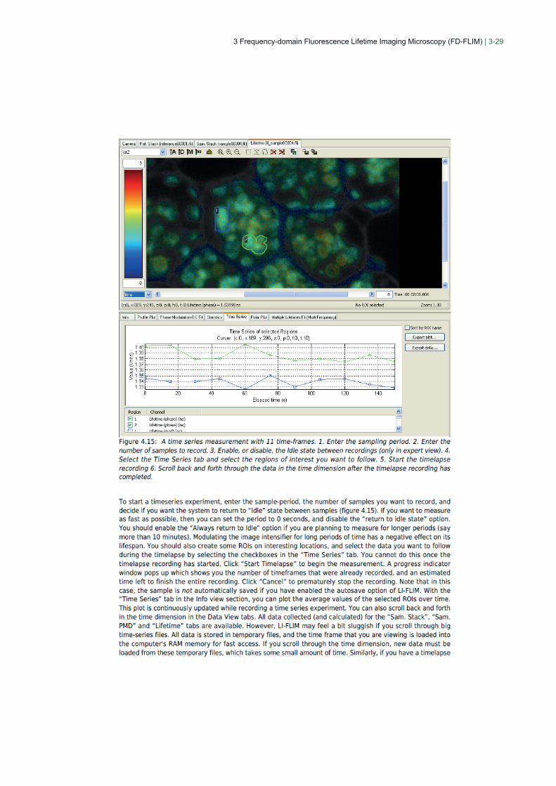
3 Frequency-domain Fluorescence Lifetime Imaging Microscopy (FD-FLIM) | 3-29

3 Frequency-domain Fluorescence Lifetime Imaging Microscopy (FD-FLIM) | 3-30

3 Frequency-domain Fluorescence Lifetime Imaging Microscopy (FD-FLIM) | 3-31

3 Frequency-domain Fluorescence Lifetime Imaging Microscopy (FD-FLIM) | 3-32

3 Frequency-domain Fluorescence Lifetime Imaging Microscopy (FD-FLIM) | 3-33
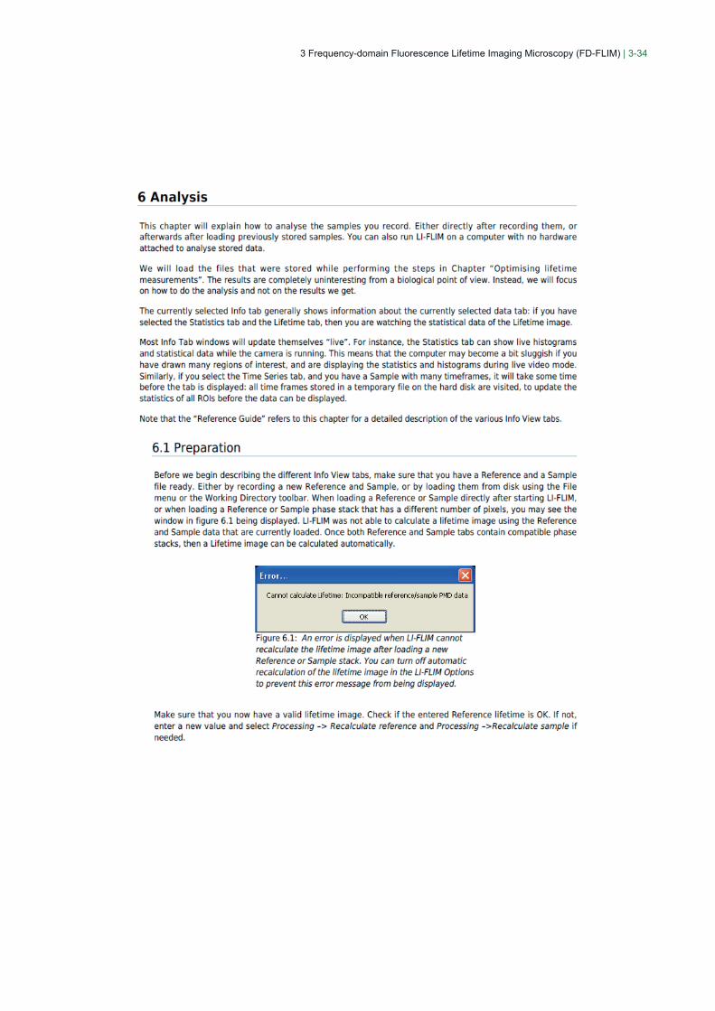
3 Frequency-domain Fluorescence Lifetime Imaging Microscopy (FD-FLIM) | 3-34
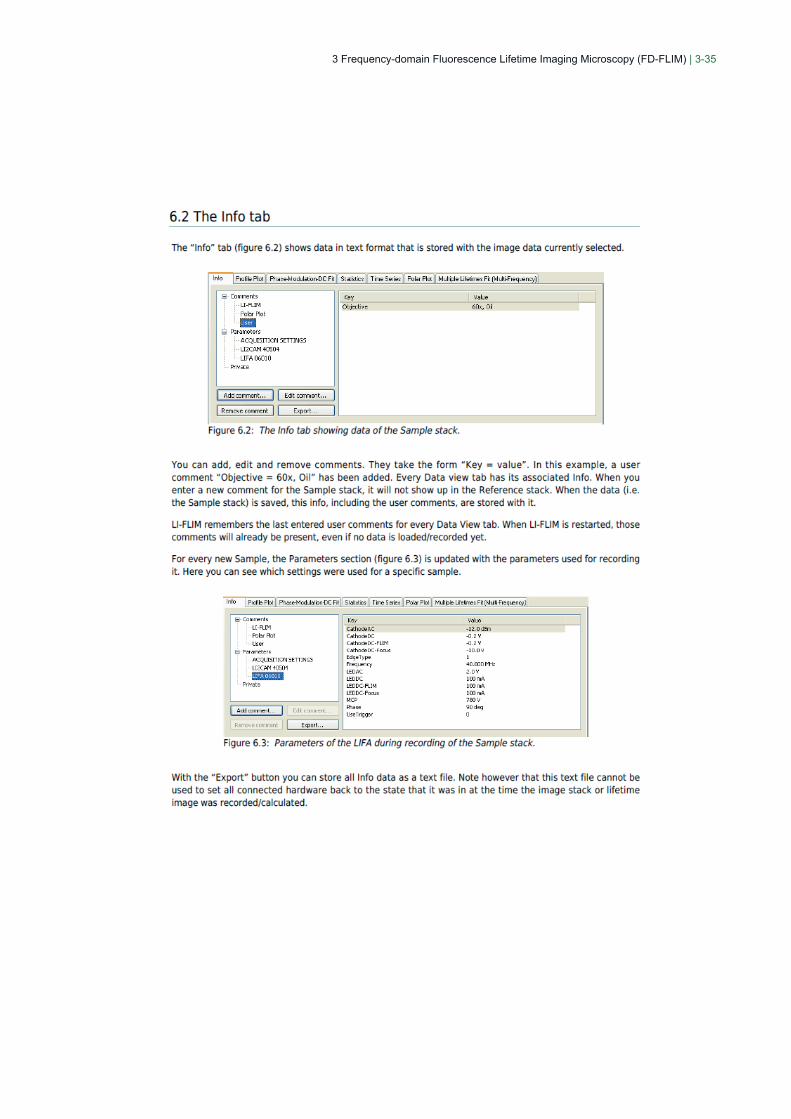
3 Frequency-domain Fluorescence Lifetime Imaging Microscopy (FD-FLIM) | 3-35

3 Frequency-domain Fluorescence Lifetime Imaging Microscopy (FD-FLIM) | 3-36

3 Frequency-domain Fluorescence Lifetime Imaging Microscopy (FD-FLIM) | 3-37

3 Frequency-domain Fluorescence Lifetime Imaging Microscopy (FD-FLIM) | 3-38

3 Frequency-domain Fluorescence Lifetime Imaging Microscopy (FD-FLIM) | 3-39

3 Frequency-domain Fluorescence Lifetime Imaging Microscopy (FD-FLIM) | 3-40
3 Frequency-domain Fluorescence Lifetime Imaging Microscopy (FD-FLIM) | 3-41
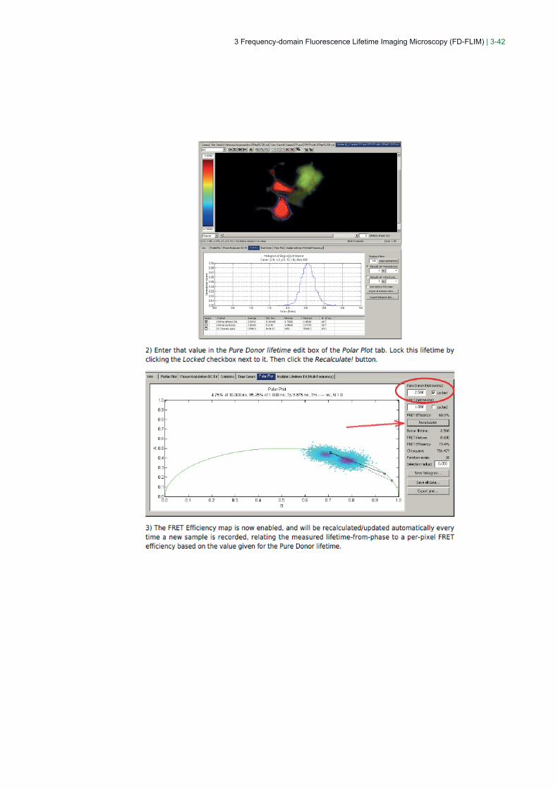
3 Frequency-domain Fluorescence Lifetime Imaging Microscopy (FD-FLIM) | 3-42

3 Frequency-domain Fluorescence Lifetime Imaging Microscopy (FD-FLIM) | 3-43

3 Frequency-domain Fluorescence Lifetime Imaging Microscopy (FD-FLIM) | 3-44
PicoQuant GmbHRudower Chaussee 2912489 BerlinGermany
Material can be downloaded from www.picoquant.com
© 2016 PicoQuant GmbHAll rights reserved. No parts of it may be reproduced, translated or transferred to third parties without written permission of PicoQuant GmbH.
www.picoquant.com