Practical Methods For Convex Multi-View Reconstruction

Practical Methods For Convex Multi-ViewReconstruction

Christopher Zach and Marc Pollefeys

ETH Zurich, Universitatstrasse 6, CH-8092 Zurich

Abstract. Globally optimal formulations of geometric computer visionproblems comprise an exciting topic in multiple view geometry. Theseapproaches are unaffected by the quality of a provided initial solution,can directly identify outliers in the given data, and provide a better the-oretical understanding of geometric vision problems. The disadvantageof these methods are the substantial computational costs, which limitthe tractable problem size significantly, and the tendency of reducinga particular geometric problem to one of the standard programs well-understood in convex optimization. We select a view on these geometricvision tasks inspired by recent progress made on other low-level visionproblems using very simple (and easy to parallelize) methods. Our viewalso enables the utilization of geometrically more meaningful cost func-tions, which cannot be represented by one of the standard optimizationproblems. We also demonstrate in the numerical experiments, that ourproposed method scales better with respect to the problem size thanstandard optimization codes.

1 Introduction

Globally optimal methods in multiple view geometry and 3D computer visionare appealing tools to estimate geometric entities from visual input. So far mostresearch in this field has been focused on the formulation of geometric visionproblems in terms of a standardized optimization taxonomy, e.g. as linear orhigher order cone programs. With very few exceptions, generic optimizationcodes are utilized for the respective numerical experiments. The emphasis onglobal optimal formulations lies on L∞-based objective functions, i.e. minimizingthe maximum over a set of convex or quasi-convex functions with respect to theunknowns. The initially intriguing L∞-based objective can be easily convertedinto a simple cost function combined with a large number of (convex) constraints,which subsequently enables tractable solvers to be applied. The decision of uti-lizing an L∞-based objective function has two important consequences: first,it induces particular (and often unrealistic) assumptions on the noise charac-teristic of the observed measurements; and second, the typically encounteredquasi-convex nature of the optimization problem implies, that the solution pro-cedure only indirectly provides the unknown variables of interest (through asequence of feasibility problems). Hence, more robust and efficient alternativeformulations of important tasks in multiple view geometry are desired.

2 Practical Methods For Convex Multi-View Reconstruction

Further, formulating geometric vision task in terms of general optimizationproblems has the advantage of having a well-understood theory and maturesoftware implementations available, but such an approach also limits the rangeof multi-view problems and objective functions to those standard optimizationproblems. In this work we propose a more direct view on a class of geomet-ric vision problems not taking the route through one of the standard convexprograms. Our view on these problems is inspired by recent advances on con-vex formulations or relaxations of low-level vision problems. Our contributionis two-fold: we demonstrate the applicability of optimization methods primarilyutilized in signal and image processing for geometric vision problems, and weextend recent convex models for multi-view reconstruction by a new cost func-tion better approximating the squared reprojection error while still preservingthe convexity of the problem.

2 Related Work

2.1 Global Optimization in Multiple View Geometry

Global optimization in multiple view geometry has gained a lot of interest in therecent years. In particular, L∞-based (or min-max) formulations are popular(i) due to the well-understood relation with fractional programming leading tolinear or second order cone programs, and (ii) due to the good accuracy providedby the solution for geometric applications if no outliers are present.

The first exposition of L∞ minimization for geometric computer vision prob-lems is given in [1], where the authors propose the L∞ cost function for multi-view reconstruction tasks. The relation between quasi-convex functions and L∞optimization for multi-view geometry was independently discovered in [2] and [3].Quasi-convex functions (i.e. functions with convex sublevel sets) can be effec-tively minimized by a bisection search for the opimal value, thus solving a se-quence of convex feasibility problems. Additional convex constraints can be alsoprovided. These approaches present structure and motion recovery given knowncamera rotations as the prototypical application.

Sim and Hartley [4] discuss an L∞ view on the problem of estimating cameracenters (again under the assumption of known rotations) given the directions ofthe baseline between cameras. The 3D scene structure is not explicitly modeledas unknown parameter subject to minimization, therefore the problem size issubstantially reduced. Placing camera centers given a set of relative directionsis similar to the graph embedding problem for motion recovery [5, 6]. In [4] thedegeneracy of embedding formulations for linear camera motions is addressedby utilizing the trifocal tensor to incorporate the relative scales of baselines.Removing the 3D structure from the problem formulation reduces the size ofthe optimization problem substantially, but also leads to minimization of quiteabstract cost functions (e.g. the angular deviation between given and estimatedbaseline directions) instead of image-related quantities like the reprojection error.

The high computational costs of L∞ optimization has lead to investigationsto reduce the respective run-time. [7] describes an interior point algorithm ex-

Practical Methods For Convex Multi-View Reconstruction 3

ploiting the same sparsity pattern in the underlying problem as it is also foundin sparse bundle adjustment methods. The observation that the objective valueof a min-max problem is only dependent on a (potentially small) subset of errorterms can be utilized to formulate faster methods for L∞ optimization [8]. Inthis approach only a subset of data points is considered for optimization (thusmaking the problem smaller), but the residuals are evaluated for all data points.If all residuals are less or equal to the objective value, then the procedure canbe stopped; otherwise additional data points with large residuals are added infurther minimization steps.

L∞ optimization has the potential disadvantage of being susceptible to out-liers in the input data. It can be shown that some of the inputs attaining themaximum error in min-max optimization are guaranteed to be outliers undersuitable assumptions, hence these outliers can be iteratively detected and re-moved by L∞ optimization [9]. Alternatively, L∞ (min-max) objective functionscan be replaced by L1 (min-sum) cost functions, leading directly to formulationsmuch less affected by outliers in the data. Straightfoward L1-based optimizationof geometric vision problems similar to many of the L∞ approaches outlinedabove usually leads to sum-of-fractions type of optimization problems, whichare extremely difficult to solve. The recent approaches described in [10, 11] (andreviewed in more detail in Sec. 3) aim on directly minimizing the number (i.e.L0-norm) of outliers for a particular inlier criterion represented by suitable (ei-ther linear or second order cone) constraints. If all data points are inliers (i.e. theresiduals are less than a given threshold), the objectve value is 0. Convexifica-tion of the L0 norm yields an L1-like objective function and thereby to respectivelinear or second order cone programs.

We present our method for practical convex optimization in multi-view geom-etry on the problem of structure and motion recovery given the global camerarotations. This raises the question of how these rotations can be determined.Global rotations can be efficiently computed from pair-wise relative orientationsbetween images by utilizing the consistency relation between relative and abso-lute camera rotations, Rj = RijRi. [12] and [13] present different methods toobtain consistent global rotations. For full structure and motion computation,[13] employs the L∞ framework of [2], but uses only a small subset of scenepoints in order to accelerate the minimization procedure and to guarantee anoutlier-free set of data points.

2.2 Non-smooth Convex Optimization and Proximal Methods

Even a convex optimization problem can be difficult to solve efficiently, especiallyif the objective is a non-smooth function. A class of methods successfully appliedin signal and image processing are based on proximal calculus: for a convexfunction f and γ > 0 the mapping

proxγf (x) = arg minx

{f(x) +

12γ‖x− x‖22

}(1)


is called the proximity operator. It generalizes the notion of projection opera-tors (for which f is the hard indicator function for a convex set S). In Eq. 1 theobjective itself is called the Moreau envelope of function f of index γ. Some-times proxγf is difficult to compute directly, but the proximity operator for theconjugate function, proxγf∗ , can be determined efficiently. In these cases we canutilize Moreau’s decomposition,

x = proxγf (x) + γ proxf∗/γ(x/γ) (2)

We refer to [14] for a recent, compact exposition of proximal calculus and itsimportance in image processing applications.

Proximal methods, in particular the forward-backward algorithm [14] andDouglas-Rachford splitting [15, 16], allow the efficient minimization of struc-tured, convex problems of the form minx f1(x) + f2(x). In brief, the Douglas-Rachford splitting iterates

x(n) = proxγf2(x(n))

x(n+1) = x(n) + proxγf1(2x(n) − x(n))− x(n), (3)

and x(n) is known to converge to the solution of minx f1(x) + f2(x). See alsoe.g. [17] for the connections between Douglas-Rachford, augmented Lagrangianand split Bregman methods. In Section 4.3 we apply the Douglas-Rachford split-ting on a problem with f2 being the indicator function of a hyper-plane (i.e.proxγf2 amounts to project the argument into a linear subspace), and f1 furtherdecomposing into many independent objectives.

3 Convex L1 Reconstruction With Known Rotations

In this section we review robust structure and motion computation with knowncamera rotations based on convex optimization. Since all the camera centersand 3D points are mutually dependent in the objective function, we choosethis application in order to demonstrate our method on a larger scale problem.Other classical problems addressed by global optimization in multi-view geom-etry are optimal point triangulation and camera resectioning, which involve amuch smaller number of unknowns. In the following we assume that global cam-era rotations are given (e.g. a set of pairwise relative rotations can be upgradedto consistent global ones via eigenvalue decomposition [13]). Let i denote theindex of the cameras and j be the index of 3D points, respectively. The setof global rotations Ri for each camera is assumed to be known. Further, letuij = (u1

ij , u2ij , 1)T be the projection of the (unknown) 3D point Xj into image

i, i.e. uij ∝ RiXj + Ti, where Ti and Xj are the translation vectors and 3Dpoint positions yet to be determined. We assume that the image coordinates uijare normalized, i.e. premultiplied by the inverse camera intrinsics. With knownrotations, the relationship between 3D structure, camera poses and image mea-surements are essentially linear (up to the unknown depth). The full projection


function

uij =RiXj + Ti

(RiXj + Ti)3

is nonlinear, but e.g. the squared reprojection error is quasi-convex and amenablefor L∞ optimization (e.g. [2]). We focus on the L1 setting where a minimizerof the sum of some deviation is sought. The intention is to increase robustnessin presence of gross outliers by utilizing an L1 objective function. [10, 11] use aquasi L∞ model by assigning zero cost, whenever the projection of a 3D point Xj

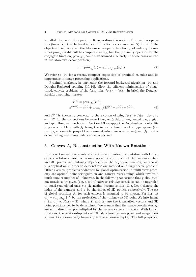
lies within a neighborhood of a user-specified radius σ (where the neighborhoodis induced either by the Euclidean norm [11] or by the maximum norm [10].Consequently, no cost is attributed in the objective function, if Xj lies within a(generalized) cone induced by the camera center Ci = −RTi Ti and the observedimage point uij (see Figure 1).

��

Ci

Xij

ωij

uij

Fig. 1. The cone induced by the camera center Ci and the observed image point uij .Points Xij residing within the shaded cone are considered as inliers and have no costin the objective function, whereas outliers are penalized.

Denoting Xij = (X1ij , X

2ij , X

3ij)

T = RiXj + Ti, the condition of Xj being inthe respective cone with radius σ reads as

‖uij −X1,2ij /X

3ij‖p ≤ σ

or equivalently,

‖uijX3ij −X

1,2ij ‖p ≤ σX

3ij , (4)

where we also employ the cheirality constraint of Xj being in front of the camerai, i.e. X3

ij ≥ 0. The underlying norm can be the L1 norm (p = 1), the Euclideanone (p = 2), or the maximum norm (p =∞). Observe that the constraint Eq. 4corresponds to a second order cone (p = 2) and the intersection of affine linearhalf-spaces, respectively.

If Ti’s and Xj ’s can be determined such that Eq. 4 is fulfilled for all i and j,then all reprojection errors are less or equal to σ (either using L2 or L∞ distancesin the image). If this is not the case, one can measure the infeasibility sij of theprojected 3D point [11],

‖uijX3ij −X

1,2ij ‖p ≤ σX

3ij + sij ,


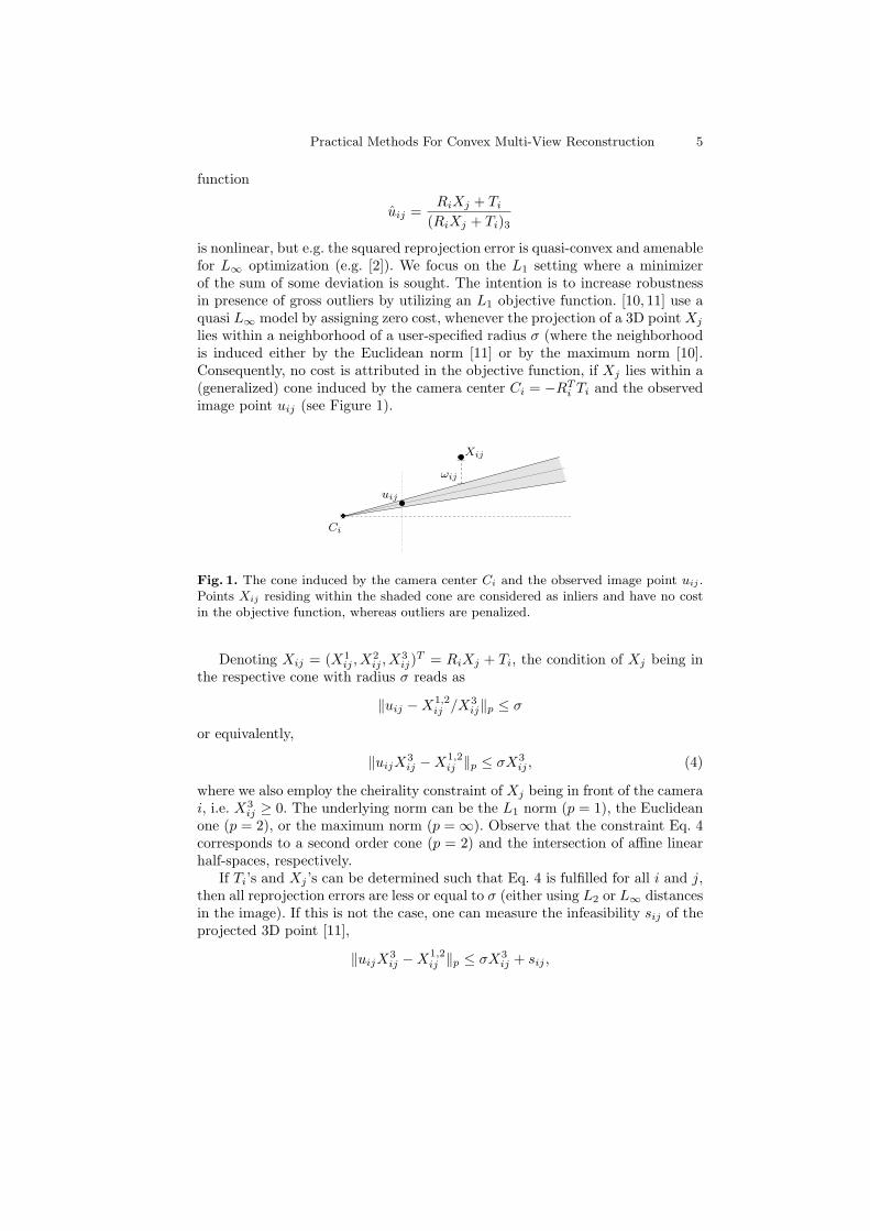
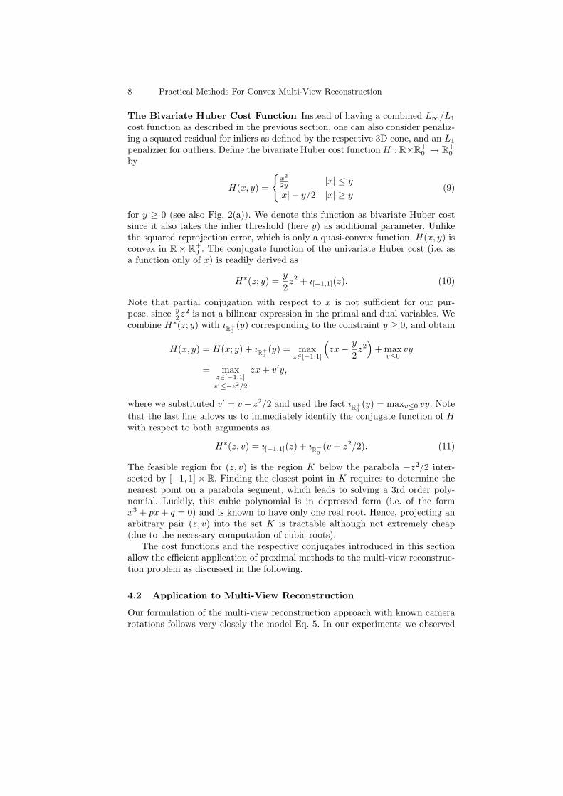
(a) g1(x, y) (b) g2(x, y) for y = 5 (c) H(x, y)

Fig. 2. Surface plots for the two pan functions g1 (a) and g2 (for a fixed value of y,(b)), and the bivariate Huber cost function (c).

or the necessary offset vectors in object space to move Xij onto the cone, ωij ∈R2 [10],

‖uijX3ij −X

1,2ij + ωij‖p ≤ σX3

ij .

Since nonzero values of sij or ωij correspond to outlier measurements in theimage, it is reasonable to search for sparse solutions in terms of sij and ωij ,respectively, i.e. to minimize the L0 norm of sij (or ωij). Convexification of theL0 norm yields the following L1 objective function and constraints (using theoffset vector formulation):

minTi,Xj ,ωij

∑ij

‖ωij‖1 s.t.

∥∥uijX3ij −X

1,2ij + ωij

∥∥p≤ σX3

ij ∀ij (5)

Xij = RiXj + Ti.

If p =∞ (and also for p = 1) this is a linear program, and for p = 2 one obtains asecond order cone program, which can be solved by suitable convex optimizationcodes.

In order to avoid the degenerate solution Ti = 0 and Xj = 0 for all camerasand 3D points in the optimization problem Eq. 5 and to avoid a 4-parameterfamily of solutions (arbitrary global translation and scale), one has to enforcesuitable cheirality constraints (e.g. X3

ij ≥ 1 [10]) or fix the reference frame [11].Utilizing the cheirality constraint implicitly selects the smallest feasible recon-struction with respect to its scale, since the objective function in Eq. 5 is reducedby decreasing the global scale.

4 Our Approach

Generic optimization of Eq. 5 using a linear or second order cone programmingtoolbox turns out to be not efficient in practice. One reason for the inefficiencyis the introduction of auxiliary variables, either sij or ωij . Another difficulty for


generic optimization codes is the large number of non-local constraints. Hence,we propose to directly optimize a non-differentiable objective function withoutthe need for additional unknowns.

4.1 The Cost Functions

In order to reformulate Eq. 5 in more general terms, we define and analyze severalconvex functions, which are used in Sec. 4.2 to derive suitable proximal-pointproblems forming the basis of the numerical scheme.

Notations We introduce the indicator function ıS(x) returning 0 if x ∈ Sand ∞ otherwise. In particular, ıR+

0and ıR−0

denote the indicator functions fornon-negative (respectively non-positive) real numbers. For a convex, lower semi-continuous function f , let f∗ be its conjugate function, f∗(z) = maxx zx− f(x).

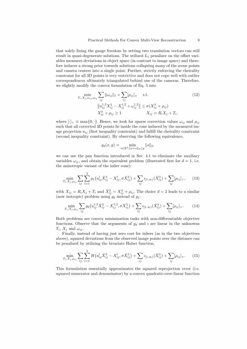
The “Pan” Functions We define the pan function gd : Rd × R+0 → R+

0 as

gd(x, y) = max {0, ‖x‖2 − y} . (6)

For a particular value of y ≥ 0 the shape of gd(·, y) is a truncated L1 cost functionresembling the cross-section of a pan-like shape (see also Fig. 2(a) and (b)). Itcan be also viewed as two-sided variant of a hinge loss function. This function isconvex, but not differentiable at ‖x‖2 = y.

As a first step to derive the conjugate function of gd, we observe that

gd(x, y) = max‖z‖2≤1

{zTx− ‖z‖2y}. (7)

Omitting the subscript in ‖·‖2 = ‖·‖, if ‖x‖ ≤ y we have zTx−‖z‖y ≤ ‖z‖ ‖x‖−‖z‖y = ‖z‖(‖x‖ − y) (by the Cauchy-Schwarz inequality), but the second factoris non-positive by assumption, hence maximizing over z in the unit disc yieldsz = 0 with objective value 0. ‖x‖ > y: observe that ‖z‖y is independent of thedirection of z and zTx is maximal if z ‖ x, i.e. z = kx for some k ∈ [0, ‖x‖−1](since ‖z‖ ≤ 1). Overall, zTx − ‖z‖y = k‖x‖2 − k‖x‖y = k‖x‖(‖x‖ − y), hencek = ‖x‖−1 (i.e. z = x/‖x‖) maximizes that expression with value ‖x‖ − y.Overall, both definitions Eqs. 6 and 7 are again equivalent.

Finally, we can convert Eq. 7 into a bilinear form by introducing the addi-tional variable v,

gd(x, y) = max‖z‖≤1,v≤−‖z‖

{zTx+ vy}. (8)

Note that gd(x, y) is ∞ for y < 0, since v is not bounded from below. For givenx ∈ Rd and y > 0 the maximization always gives v = −‖z‖, since the objectivecan be increased whenever v < −‖z‖. Thus, the definitions in Eqs. 7 and 8are equal, and Eq. 8 allows us to directly read off the corresponding conjugatefunction g∗d(z, v) = ıCd

(z, v) with Cd ≡ {(z, v) : ‖z‖ ≤ 1, ‖z‖ ≤ −v}. Thus, wecan reduce the computation of proxγgd

essentially to the projection into the setCd in view of Moreau’s decomposition Eq. 2. Projecting into Cd can be done inclosed form and distiction of cases.


The Bivariate Huber Cost Function Instead of having a combined L∞/L1

cost function as described in the previous section, one can also consider penaliz-ing a squared residual for inliers as defined by the respective 3D cone, and an L1

penalizier for outliers. Define the bivariate Huber cost function H : R×R+0 → R+

0

by

H(x, y) =

{x2

2y |x| ≤ y|x| − y/2 |x| ≥ y

(9)

for y ≥ 0 (see also Fig. 2(a)). We denote this function as bivariate Huber costsince it also takes the inlier threshold (here y) as additional parameter. Unlikethe squared reprojection error, which is only a quasi-convex function, H(x, y) isconvex in R × R+

0 . The conjugate function of the univariate Huber cost (i.e. asa function only of x) is readily derived as

H∗(z; y) =y

2z2 + ı[−1,1](z). (10)

Note that partial conjugation with respect to x is not sufficient for our pur-pose, since y

2z2 is not a bilinear expression in the primal and dual variables. We

combine H∗(z; y) with ıR+0

(y) corresponding to the constraint y ≥ 0, and obtain

H(x, y) = H(x; y) + ıR+0

(y) = maxz∈[−1,1]

(zx− y

2z2)

+ maxv≤0

vy

= maxz∈[−1,1]

v′≤−z2/2

zx+ v′y,

where we substituted v′ = v− z2/2 and used the fact ıR+0

(y) = maxv≤0 vy. Notethat the last line allows us to immediately identify the conjugate function of Hwith respect to both arguments as

H∗(z, v) = ı[−1,1](z) + ıR−0(v + z2/2). (11)

The feasible region for (z, v) is the region K below the parabola −z2/2 inter-sected by [−1, 1] × R. Finding the closest point in K requires to determine thenearest point on a parabola segment, which leads to solving a 3rd order poly-nomial. Luckily, this cubic polynomial is in depressed form (i.e. of the formx3 + px+ q = 0) and is known to have only one real root. Hence, projecting anarbitrary pair (z, v) into the set K is tractable although not extremely cheap(due to the necessary computation of cubic roots).

The cost functions and the respective conjugates introduced in this sectionallow the efficient application of proximal methods to the multi-view reconstruc-tion problem as discussed in the following.

4.2 Application to Multi-View Reconstruction

Our formulation of the multi-view reconstruction approach with known camerarotations follows very closely the model Eq. 5. In our experiments we observed


that solely fixing the gauge freedom by setting two translation vectors can stillresult in quasi-degenerate solutions. The utilized L1 penalizer on the offset vari-ables measures deviations in object space (in contrast to image space) and there-fore induces a strong prior towards solutions collapsing many of the scene pointsand camera centers into a single point. Further, strictly enforcing the cheiralityconstraint for all 3D points is very restrictive and does not cope well with outliercorrespondences ultimately triangulated behind one of the cameras. Therefore,we slightly modify the convex formulation of Eq. 5 into

minTi,Xj ,ωij ,ρij

∑ij

‖ωij‖1 +∑ij

[ρij ]+ s.t. (12)

∥∥u1,2ij X

3ij −X

1,2ij + ω1,2

ij

∥∥ ≤ σ(X3ij + ρij)

X3ij + ρij ≥ 1 Xij = RiXj + Ti,

where [·]+ ≡ max{0, ·}. Hence, we look for sparse correction values ωij and ρijsuch that all corrected 3D points lie inside the cone induced by the measured im-age projection uij (first inequality constraint) and fulfill the cheirality constraint(second inequality constraint). By observing the following equivalence,

gd(x, y) = mins∈Rd:‖x+s‖2≤y

‖s‖2,

we can use the pan function introduced in Sec. 4.1 to eliminate the auxiliaryvariables ωij , and obtain the equivalent problem (illustrated first for d = 1, i.e.the anisotropic variant of the inlier cone):

minTi,Xj ,ρij

∑ij

2∑l=1

g1(ulijX

3ij −X l

ij , σX3ij

)+∑ij

ı[1,∞)(X3ij) +

∑ij

[ρij ]+, (13)

with Xij = RiXj + Ti and X3ij = X3

ij + ρij . The choice d = 2 leads to a similar(now isotropic) problem using g2 instead of g1:

minTi,Xj ,ρij

∑ij

g2(u1,2ij X

3ij −X

1,2ij , σX

3ij

)+∑ij

ı[1.∞)(X3ij) +

∑ij

[ρij ]+. (14)

Both problems are convex minimization tasks with non-differentiable objectivefunctions. Observe that the arguments of gd and ı are linear in the unknownsTi, Xj and ωij .

Finally, instead of having just zero cost for inliers (as in the two objectivesabove), squared deviations from the observed image points over the distance canbe penalized by utilizing the bivariate Huber function,

minTi,Xj ,ρij

∑ij

2∑l=1

H(ulijX

3ij −X l

ij , σX3ij

)+∑ij

ı[1,∞)(X3ij) +

∑ij

[ρij ]+. (15)

This formulation essentially approximates the squared reprojection error (i.e.squared numerator and denominator) by a convex quadratic-over-linear function


for inlier points. Consequently, the 3D points in the corresponding solution tendto stay closer to the observed image measurements. More importantly, inlier3D points are attracted by a unique minimum and the numerical procedureconverges faster in practice.

At the first glance nothing is gained by such reformulation other than movingthe (linear or second order cone) constraints into the objective (Eqs. 13 and 14),and allowing for a refined cost for inlier points (Eq. 15). But the problems arevery structured: the objective function is a sum of many convex functions onlytaking very few arguments, therefore depending only on a small subset of theunknowns. Hence, a variant of Douglas-Rachford splitting can be applied asdecribed in the following section.

4.3 Numerical Scheme

The objective functions in the previous section can be more generally written as

minX

∑k

hk(LkX ), (16)

where X denotes all unknowns Ti, Xj and ρij , the hk are convex functions and Lkare matrices of appropriate dimensions. Similar to dual decomposition methodswe can introduce local unknowns xk for each hk and explicitly enforce globalconsistency (see also [18]),

minX ,Yk

∑k

hk(Yk)︸︷︷︸≡f1

+∑k

ı{LkX = Yk}︸︷︷︸≡f2

. (17)

Application of Douglas-Rachford splitting amounts to solving proxγf1 and proxγf2(recall Eq. 3). The first proximity operator, proxγf1 decouples into independentproblems proxγhk

, in particular (referring to Eq. 15, with analogous expressionsfor Eqs. 13 and 14) the term hk(LiX ) is one of

hk(LiX ) =

H(ulijX

3ij −X l

ij , σX3ij

)l ∈ {1, 2}

ı[1,∞)(X3ij)

[ρij ]+

For hk equal to gd or H we can utilize the derivations from Section 4.1 in order todetermine proxγgd

or proxγH efficiently. If hk = ı[1,∞)(·), the proximity operatorcan be easily derived as clamping operation into the feasible domain [1,∞), andfor hk = [·]+ the respective proximity operator is given by

proxγ[·]+(x) = max(0, x− γ).

proxγf2(X , (Yk)k) corresponds to finding the closest point (X , (Yk)k) satisfyingthe linear constraints LkX = Yk for all k, therefore proxγf2 is a projection op-eration into a linear subspace. Following [19] a particular instance of a Douglas-Rachford approach called simultaneous-direction method of multipliers (SDMM)


can be stated: choose γ > 0 and arbitrary initial values y(0)k and z(0)

k , and iteratefor n = 0, 1, . . .:

x(n) =

(∑k

LTk Lk

)−1∑k

LTk

(y(n)k − z(n)

k

)y(n+1)k = proxγhk

(Lkx

(n) + z(n)k

)∀k (18)

z(n+1)k = z

(n)k + Lkx

(n) − y(n+1)k ∀k.

x(n) converges to a solution of Eq. 16. Note that the Lk are very sparse matri-ces, and the inverse of

∑LTk Lk can be efficiently found using sparse Cholesky

factorization. Note that a projection into a linear subspace is always uniquelydefined, hence

∑LTk Lk must have full rank.

Since the method is iterative, a suitable stopping criterion is required. Weselected the following one: the current 3D structure and the one obtained aftera significant number of iterations (our choice is 1000) are normalized in theirsizes, and the maximum change in the respective 3D point positions is usedas stopping criterion. If no 3D point was moved more than ε, then the updateiterations terminate. We use ε = 10−8 in our implementation. Further, we setγ = 0.1 in all experiments.

5 Numerical Results

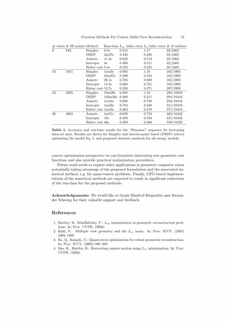
Most work in convex and quasi-convex optimization in multiple view geometryuses the “Dinosaur” data-set1 consisting of camera poses and tracked 2D points.We use the rotations known from the given projection matrices, and determinethe 3D structure and camera centers using the convex formulations describedin Sec. 4.2. We obtain numerical and timing results for several optimizationcodes: (i) we utilize an easy-to-use simplex-based linear program solver2 to op-timize the problem Eq. 5 (denoted as “Simplex” in the evaluation Table 1); (ii)we also experiment with an interior point algorithm for semi-definite programs(DSDP [20], which has also a direct interface to specify LP cones, indicated byDSDP in Table 1)); and finally we implemented the update equations Eq. 18 forthe described cost functions to minimize the respective energy. Table 1 summa-rizes the obtained timing and accuracy results, where we set the inlier radius σto one pixel. Of particular interest in the evaluation is the dependence of the run-time on the data-set size: generally, the iterative proximal methods scale betterwith the data-set size. Both generic LP solvers were not able to complete thefull data-set (due to numerical instabilities for the Simplex method and excessivememory consumption of the semi-definite code DSDP).

These performance numbers need to be compared with the close to two hoursreported in [11] for the full data-set. Note that [10] does not indicate the respec-tive run-time performance. The Huber function based model Eq 15 is strictly1 available from http://www.robots.ox.ac.uk/˜vgg/data/data-mview.html2 http://lpsolve.sourceforge.net/


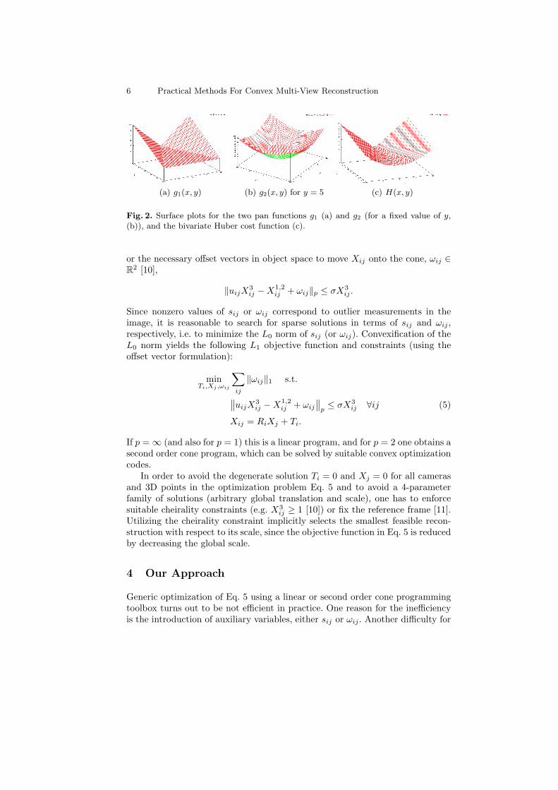
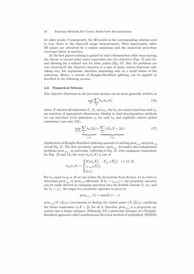
(a) “Dinosaur” (b) “Church” (c) “Building”

Fig. 3. Reconstruction result for the “Dinosaur” data set (36 images, ≈ 5.000 3Dpoints), “Church” data set (58 views, ≈ 12.500 3D points), and “Building” (128 images,≈ 27.000 3D points) using the energy function Eq 15. No bundle adjustment is applied.

convex for inlier points (and therefore has a unique minimizer), which could bethe explanation for reaching the stopping criterion faster than the other energymodels Eqs. 13 and 14.

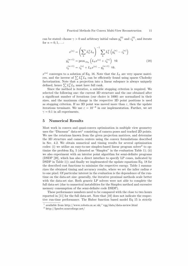
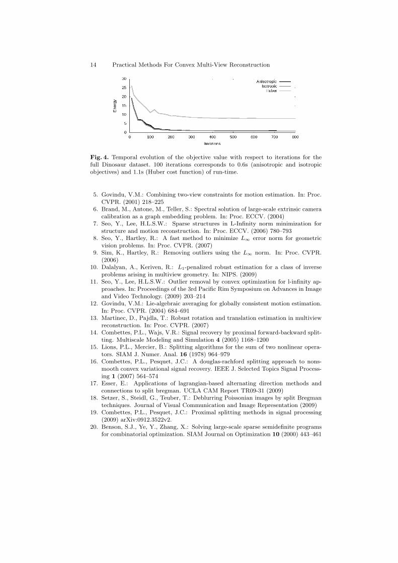
Since the Huber cost model Eq. 15 penalizes deviations from the ray inducedby the image measurements, the final reprojection error of the 3D points areconsistently smaller than for the combined L∞/L1 cost models. The last columnin Table 1 depicts the number of reported outlier measurements outside the re-spective σ radius in the image. This value is stated to show the equivalence of theiterative method for Eq. 13 with the linear programming formulation. Further,it shows that the smaller reprojection error in the Huber cost model is compen-sated by a larger number of reported outliers (which is a result of the energymodel and not induced by the implementation). We also applied the proposedmethod on real-world data sets consisting of 58 and 128 views, respectively (seeFig. 3(b) and (c)). Consistent rotations are estimated via relative poses fromSIFT feature matches. The iterative Huber approach (for σ = 2 pixels) requires12.5 and 40 minutes to satisfy the convergence test, and about 30% is spent inapproximate column reordering for the sparse Cholesky factorization. The meanreprojection errors for inliers are 1.08 and 0.53 pixels, respectively. Figure 4 de-picts the convergence rate of the objective value for the Dinosaur data set withrespect to the number of iterations. Since the objective function is rather flatnear the global minimum, small changes in the objective value do not necessarilyimply small updates in the variables, and the termination criterion is achievedmuch later.

6 Conclusion

In this work we present a different view on convex problems arising in mutiple-view geometry, and propose a non-standard optimization method for these prob-lems. By looking at classical optimization tasks in geometric vision from a general


# views # 3D points Method Run-time L∞ inlier error L2 inlier error # of outliers

8 843 Simplex 9.5s 0.913 1.17 33/2465DSDP 2m27s 0.430 0.480 33/2465Anisotr. 11.4s 0.622 0.712 33/2465Isotropic 4s 0.466 0.511 32/2465Huber cost 5.4s 0.223 0.235 48/2465

16 1915 Simplex 1m43s 0.892 1.10 165/5905DSDP 24m37s 0.389 0.434 165/5905Anisotr. 26.1s 0.705 0.800 165/5905Isotropic 13.5s 0.668 0.721 165/5905Huber cost 13.7s 0.256 0.271 207/5905

24 3205 Simplex 19m26s 0.895 1.10 294/10416DSDP 103m36s 0.369 0.411 294/10416Anisotr. 1m44s 0.895 0.756 294/10416Isotropic 1m33s 0.784 0.838 311/10416Huber cost 1m16s 0.262 0.278 371/10416

36 4983 Anisotr. 1m51s 0.650 0.734 383/16432Isotropic 45s 0.483 0.533 421/16432Huber cost 46s 0.269 0.286 539/16432

Table 1. Accuracy and run-time results for the “Dinosaur” sequence for increasingdata-set sizes. Results are shown for Simplex and interior-point based (DSDP) solversoptimizing the model Eq. 5, and proposed iterative methods for all energy models.

convex optimization perspective we can formulate interesting new geometric costfunctions and also provide practical minimization procedures.

Future work needs to explore other applications in geometric computer visionpotentially taking advantage of the proposed formulation and the associated nu-merical method, e.g. for quasi-convex problems. Finally, GPU-based implemen-tations of the numerical methods are expected to result in significant reductionsof the run-time for the proposed methods.

Acknowledgements: We would like to thank Manfred Klopschitz and Alexan-der Schwing for their valuable support and feedback.

References

1. Hartley, R., Schaffalitzky, F.: L∞ minimization in geometric reconstruction prob-lems. In: Proc. CVPR. (2004)

2. Kahl, F.: Multiple view geometry and the L∞ norm. In: Proc. ICCV. (2005)1002–1009

3. Ke, Q., Kanade, T.: Quasiconvex optimization for robust geometric reconstruction.In: Proc. ICCV. (2005) 986–993

4. Sim, K., Hartley, R.: Recovering camera motion using L∞ minimization. In: Proc.CVPR. (2006)


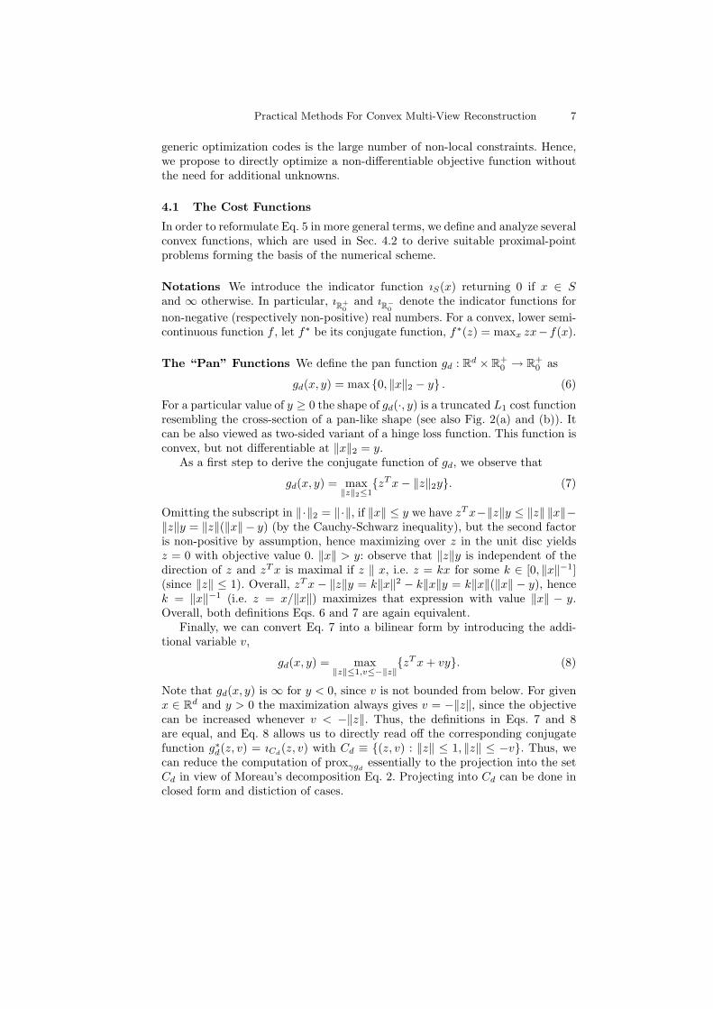
Fig. 4. Temporal evolution of the objective value with respect to iterations for thefull Dinosaur dataset. 100 iterations corresponds to 0.6s (anisotropic and isotropicobjectives) and 1.1s (Huber cost function) of run-time.

5. Govindu, V.M.: Combining two-view constraints for motion estimation. In: Proc.CVPR. (2001) 218–225

6. Brand, M., Antone, M., Teller, S.: Spectral solution of large-scale extrinsic cameracalibration as a graph embedding problem. In: Proc. ECCV. (2004)

7. Seo, Y., Lee, H.L.S.W.: Sparse structures in L-Infinity norm minimization forstructure and motion reconstruction. In: Proc. ECCV. (2006) 780–793

8. Seo, Y., Hartley, R.: A fast method to minimize L∞ error norm for geometricvision problems. In: Proc. CVPR. (2007)

9. Sim, K., Hartley, R.: Removing outliers using the L∞ norm. In: Proc. CVPR.(2006)

10. Dalalyan, A., Keriven, R.: L1-penalized robust estimation for a class of inverseproblems arising in multiview geometry. In: NIPS. (2009)

11. Seo, Y., Lee, H.L.S.W.: Outlier removal by convex optimization for l-infinity ap-proaches. In: Proceedings of the 3rd Pacific Rim Symposium on Advances in Imageand Video Technology. (2009) 203–214

12. Govindu, V.M.: Lie-algebraic averaging for globally consistent motion estimation.In: Proc. CVPR. (2004) 684–691

13. Martinec, D., Pajdla, T.: Robust rotation and translation estimation in multiviewreconstruction. In: Proc. CVPR. (2007)

14. Combettes, P.L., Wajs, V.R.: Signal recovery by proximal forward-backward split-ting. Multiscale Modeling and Simulation 4 (2005) 1168–1200

15. Lions, P.L., Mercier, B.: Splitting algorithms for the sum of two nonlinear opera-tors. SIAM J. Numer. Anal. 16 (1978) 964–979

16. Combettes, P.L., Pesquet, J.C.: A douglas-rachford splitting approach to nons-mooth convex variational signal recovery. IEEE J. Selected Topics Signal Process-ing 1 (2007) 564–574

17. Esser, E.: Applications of lagrangian-based alternating direction methods andconnections to split bregman. UCLA CAM Report TR09-31 (2009)

18. Setzer, S., Steidl, G., Teuber, T.: Deblurring Poissonian images by split Bregmantechniques. Journal of Visual Communication and Image Representation (2009)

19. Combettes, P.L., Pesquet, J.C.: Proximal splitting methods in signal processing(2009) arXiv:0912.3522v2.

20. Benson, S.J., Ye, Y., Zhang, X.: Solving large-scale sparse semidefinite programsfor combinatorial optimization. SIAM Journal on Optimization 10 (2000) 443–461

Documents

Practical Methods For Convex Multi-View Reconstruction